b-spline curve fitting: application to cartographic ... · b-spline curve fitting: application to...

B-spline Curve Fitting:Application to Cartographic Generalization of Maritime Lines

Eric Saux

Institut de Recherche en Informatique de NantesNantes, France

Abstract

Generalization is the process of abstraction applied when the scaleof a map is changed. It involves modifications of data in such a waythat the data can be represented in a smaller space, while best pre-serving geometric as well as descriptive characteristics. A map isan abstracted model representing the geometric reality. The smallerthe scale, the more schematic the representation. Line cartographicgeneralization deals with graphic representation of lines. Many al-gorithms are available for an automated line cartographic general-ization. Instructions for using these algorithms are often complexand representations applied ill-adapted to some generalization pro-cesses. In this paper, we explain the advantages of using B-splinecurves in a line generalization process. We focus on processing ofline cartographic generalization operators in a maritime context.

Keywords: Line cartographic generalization, B-spline curve.

1 INTRODUCTION

We need to distinguish between the generalization issues that arebrought about by graphic representation from those which arisefrom modelling at different levels of spatial and semantic resolu-tion. Second generalization can be viewed as a series of trans-formations (in some graphic representation of spatial information),intended to improve data legibility and understanding, and per-formed with respect to the interpretation which defines the end-product. These two categories have motivated research mainlyin two areas: model-oriented generalization, with focus on thefirst stage above-mentioned, and cartographic generalization, whichdeals with graphic representation. Our paper is relevant to carto-graphic generalization.

Cartographic generalization includes the whole processings en-countered when the scale of the map is changed into a smallerscale. We should produce a legible map which is as close as pos-sible from reality. The tools currently available for automated car-tographic generalization resemble those of the manual generaliza-tion. A catalogue of cartographic generalization operators has beenproposed [23], including selection/elimination, aggregation, struc-turing, compression (or filtering), smoothing, exaggeration, carica-turing, enlargement and displacement. One can essentially distin-guish between two approaches for the implementation of the work-ing tools in generalization. One is automatic while the other is in-teractive. The generalization automation has been studied for overtwenty years. The difficulties of providing an automatic solutionpoints out the complexity of the problem.

The second section of the paper deals with the representationsused for data modelling. Subsection 2.1 is devoted to the represen-tation by means of a list of points. Most generalization algorithmshave been developed focusing on the manipulation of vectors. Rep-resentation by means of a list of points does not provide fair mod-

elling of curves which may have complex and varying shapes. Inaddition, this representation is often ill-adapted to some generaliza-tion process. In subsection2.2, we suggest a different representationbased on B-spline curves.

The third section of the paper deals with the application of B-spline representation in processing of line cartographic generaliza-tion operators in a maritime context. In subsection 3.1, we focusour attention on data compression using a bisection method on thenumber of control points. Line smoothing and displacement opera-tors are developed in subsection 3.2. The strategy is based on a me-chanical approach. The curve displacement is obtained through thedisplacement of control points. Internal and external forces are ap-plied at control points in order to produce the desired deformation.Lastly, we introduce a technique for curve aggregation (subsection3.3).

2 GEOMETRIC DATA MODELLING

2.1 Representation by means of a list of points

Polygonal curves are often encountered for data modelling. Theyare appropriate to data compression as well as to simplicity and ef-ficiency (CPU time) of their algorithms [25].

Data compression algorithms based on polygonal curves cor-respond to the first generalization algorithms. Cartographer werequickly aware that cartographic results were not sufficient usingthese algorithms. Research in automatic generalization turned toother algorithms permitting displacements. The goals were essen-tially smoothing and caricaturing.

Three trends can be emphasized for smoothing. We can citesmoothing methods based on averaging, convolution or neighbour-ing points. Averaging techniques [3, 19] smooth small details whilepreserving the general shape. Algorithms considering convolution,gaussian smoothing for example [2, 18], are more regular. They areused for smoothing details which have the same size. At the op-posite, smoothing algorithms based on neighbouring points [6, 27]have little influence on lines which are defined with a high densityof points.

Dutton’s algorithm [8] corresponds to the Brophy inversesmoothing algorithm [3]. Increasing the angularity is not a com-mon practice in generalization. Lowe’s algorithm [18] is moreinteresting. Tests display its interest for smoothing by limitingdeviations and for caricaturing [22]. Nevertheless, the choice ofthe parameters is difficult.

Generalization algorithms are usually based on a representationby means of a list of points. The result quality depends on the linemorphology [4]. In practice, one of the solutions often encounteredconsists of combining a simplification and a smoothing process: forexample, Douglas and Peucker’s algorithm [7] is followed by a cu-bic spline computation. At the present time, one should have an em-

International Conference Graphicon 1998, Moscow, Russia, http://www.graphicon.ru/

piric approach for determining a solution (choice of an algorithmand its parameter values). It is natural to notice the high cost of sucha technique.

More generally, this representation is not sufficient:

� for the acceptance of some resulting displayed curves,

� as a general representation method.

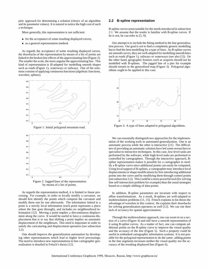
As regards the acceptance of some resulting displayed curves,the drawbacks of the representation by means of a list of points arelinked to the broken line effects of the approximating line (Figure 2).The smaller the scale, the more angular the approximating line. Thiskind of representation is ill-adapted for modelling smooth shapessuch as roads (Figure 1), waterways or railways. One of the solu-tions consists of applying continuous functions (algebraic functions,wavelets, splines).

0 10.5

0.2

0.3

0.4

0.5

0.6

0.7

0.8

0.9

Figure 1: Initial polygonal mountain road.

0 10.5

0.2

0.3

0.4

0.5

0.6

0.7

0.8

0.9

Figure 2: Jagged lines of the representationby means of a list of points.

As regards the representation method, it is limited to linear pro-cessing. For example, in order to locally modify a curvature, weshould first identify the points which compose the curvature andmodify them one by one afterwards. The information linked to apoint is a strictly local information (each point represents a placewhere the line goes through), and includes no neighbourhood in-formation [12]. Moving a point implies a discontinuous displace-ment along the curve. It would be useful to have a continuous dis-placement that is to say that shifting a point implies an automaticdisplacement of the neighbours. This need is important in order tosatisfy the caricaturing and displacement operators (see subsection3.2).

One should improve the generalization automation by develop-ing other representations which lead to higher level processings.The need to introduce new representations in line cartographic gen-eralization is detailed in Fritsch’s thesis [12].

2.2 B-spline representation

B-spline curves seem suitable for the needs introduced in subsection2.1. We assume that the reader is familiar with B-spline curves. Ifhe is not, he can refer to [5, 9].

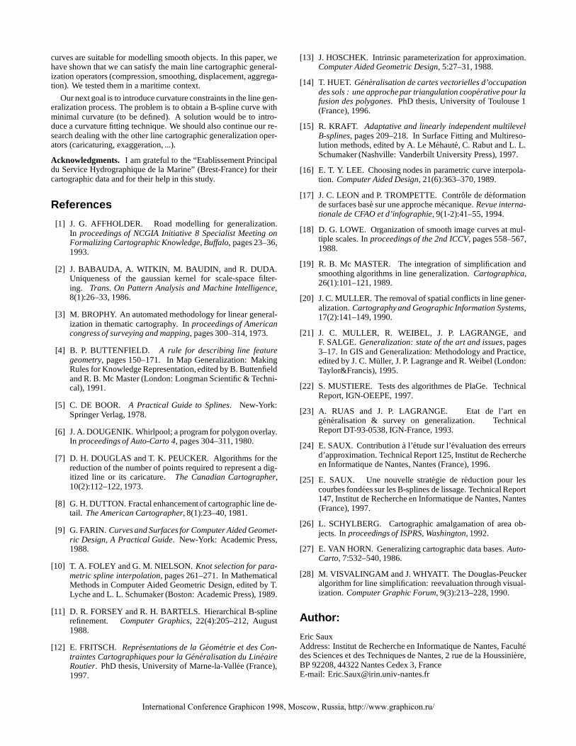
Our attempt is to include the fitting method in the line generaliza-tion process. Our goal is not to find a completely generic modellingbut to find the best modelling for a type of lines. As B-spline curvesare smooth curves, they are well-adapted for modelling smooth linessuch as roads (Figure 1), railways or waterways (see also [1]). Onthe other hand, geographic features such as seaports should not bemodelled with B-splines. The jagged line of a pier for exampleshould remain in the generalized map (Figure 3). Polygonal algo-rithms ought to be applied in this case.

20 30 4025 35

60

55

65

Figure 3: A type of lines adapted to polygonal algorithms.

We can essentially distinguish two approaches for the implemen-tation of the working tools in automated generalization. One is anautomatic process while the other is interactive [21]. The difficul-ties of providing an automatic solution have led some researchers tospecialize in interactive techniques. In this case, low-level tasks areperformed by the software, while high-level tasks are performed orcontrolled by cartographers. Through the interactive approach, B-spline representation makes it possible for a cartographer to mod-ify a B-spline curve since additional points can easily be computed.Using local support of B-splines, a cartographermay introduce localdisplacements or shape modifications by first introducing additionalpoints into the curve and by modifying them through control points(see subsection 3.2). This could be a more powerful tool (for solvingline self-intersection problem for example) than the usual strategiesbased on a simple shifting of data points.

In addition, B-spline parameters are invariant with respect toaffine transformations. As a result, B-splines are well-adapted tomultiresolution problems [11, 15]. Fritsch explains in his thesis theadvantage of wavelets in this context. He explains their drawbacksfor solving generalization operators as well [12]. We can cite theirlack of accuracy for spatial approximation.

Through the multiresolution approach, one can zoom in on a sec-tion of a curve (Figure 4) and still have a smooth representation ofit using B-spline curves. As a matter of fact, one can compute ad-ditional points on the B-spline curve to improve the visual qualityand the accuracy of the line (Figure 5). Such a property could beuseful in embarked cartographic information systems. It is not pos-sible for the polygonal representation to do the same: adding pointsin the line segments increases neither the visual quality nor the ac-curacy of the resulting displayed line (Figure 6).


0 10 20 30 40 50 60 70 80

10

20

30

40

50

60

Figure 4: Initial polygonal line (1355 points).

25 26 27 28 29 30

40

41

42

43

40.5

41.5

42.5

43.5

Figure 5: Interest of B-spline curves for curve section analysis.

25 26 27 28 29 30

40

41

42

43

40.5

41.5

42.5

Figure 6: Drawback of piecewise linear curves forcurve section analysis.

In the next section we explain how B-spline curves can be in-cluded in the cartographic generalization process by studying thegeneralization operators corresponding to the maritime context.

3 MARITIME LINE CARTOGRAPHIC GEN-ERALIZATION

The main generalization operators in this context are:

� compression,� smoothing,� displacement,� aggregation.

The lines we study are isobathymetric lines1 or coastlines. Themain constraint we should take into account in the modelling pro-cess is safety. Priority is to ensure safety. That is to say for coast-lines, it is less dangerous for sailors if the land is shifted inside thesea than the opposite. We study the four operators in the followingsubsections.

1line whose points correspond to the same value in depth

3.1 Data compression

Let P be the polygonal curve defined by the “original” given pointspi. The general problem of data compression (or reduction) isto define a curve f with a minimal number of parameters so thatd(P;f) � " (d being a criterion for estimating data approximation[24]). In practice, tolerance " is chosen so that there is no visual dif-ference between P and f for the given representation scale.

The advantage of using B-spline curves for data compression isto be able to deal with both compression and smoothing. In [25] wecompare our method to some polygonal methods and spline meth-ods (knot removal methods). Good results are obtained with respectto compression rate and computation cost.

Fitting B-splines are suitable for geographic data reduction. Datausually come from a digitizing process. This leads to digitizing er-rors. We assume that these are removed by a “cleaning” process.This involves the removalof spurious elements such as peaks, loops,duplicates and other redundant data. Nevertheless, noise cannot betotally removed, requiring application of fitting techniques.

We have to determine the minimum number of control pointsso that the corresponding B-spline approximation yields an errorsmaller than (or equal to) tolerance ". A reasonable assumption isthat the error in the approximating process increases as the numberof control points decreases. An approximating B-spline curve is de-fined by solving a linear system of equations (least squares fittingtechnique). If we start by letting n (n being the number of the givenpoints) the number of control points of B-spline curve f (the inter-polating curve is assumed to be the curve of reference), the num-ber of control points can then be determined applying a bisectionmethod [25]. It may happen that a high number of points yields aninitial system of non-maximum rank. In such a case, the initial num-ber of control points is chosen slightly smaller than n.

In [25] we explain the particular choices of knot vector T , pa-rameter values �i, order k leading to fair approximation. We brieflysummarize the results. Fair approximation leading to high datacompression rates are obtained with:

� a uniform knot vector T ,� Hoschek’s intrinsic parameterization [13],� an order 4 (cubic B-spline curves).

In cartography, processing time should be the lowest. That iswhy we advise rather using a centripetal parameterization [16] thanHoschek’s intrinsic parameterization. It yields a good compromisebetween reduction and processing time.

We have compared our strategy with polygonal compressionmethods such as Douglas and Peucker’s algorithm [7]. The choiceof this algorithm can be explained by first its interest in cartogra-phy and its ability to obtain high compression rates. The successof Douglas and Peucker’s filtering algorithm in cartography may beexplained by the fact that the points it selects approximate the linevertices quite well. It tends to select critical points close to those se-lected by humans. However, the problem is that this algorithm cancreate self-intersecting lines while increasing " because no mecha-nism is included for discarding topologic inconsistencies. Further-more, overlaps might result between different lines as a result offiltering each line individually (Figure 8). Results show that ourmethod is well-adapted to smooth lines [25] by:

� improving the visual quality of the resulting displayed im-age by reducing without solving the self-intersecting problem(Figure 9),

� having equivalent or higher compression rates [25] (Figure 9).

In both cases, considering the algorithm with smaller tolerances mayreduce the topologic errors [20, 28].


10 2015

26

27

28

29

30

31

32

33


10 2015

26

27

28

29

30

31

32

33Douglas & Peucker (compression: 93%)

Figure 8: Approximating polygonal curve.

10 2015

26

27

28

29

30

31

32

33Fitting technique (compression: 94%)

Figure 9: Approximating B-spline curve(with the same " as in fig. 8).

Our data compression method could be considered as an elemen-tary cartographic generalization system: results obtained by havinglesser accuracy (or higher tolerance ") lead to data compression andline smoothing (Figures 10, 11 and 12). We should now introduceadditional generalization operators (displacement, exaggeration, ...)in order to improve the method. The results differ according to theapplying order of the different operators [14].

80 90 100 11085 95 105

30

40

25

35

45


80 90 100 11075 85 95 105

30

40

25

35

45

Figure 11: Generalized line obtained using our data compressionalgorithm while increasing " (" = 0:2mm).

80 90 100 11075 85 95 105

30

40

25

35

45

Figure 12: Generalized line obtained using our data compressionalgorithm while increasing " (" = 0:4mm).

3.2 Line smoothing and displacement

The goal of this section is to deal with smoothing and displacementcartographic operators. The smoothing process should preserve thevertices of the initial line. Both of them should ensure safety that isto say that each curve ought to be shifted towards deeper areas. Letus propose a rough draft of what is expected (Figure 13).

Generalized line (smoothing and displacement)

Initial line

Direction ofhigher depth

Figure 13: Manual curve smoothing and displacement.

Intuitively, one should:

� produce an approximating curve f which is as close as pos-sible from “original” vertices (which are on the right side orsafety side),

� apply forces at specific locations to shift curve f towardssafety.

The first stage could be achieved applying weighted fitting tech-niques. These techniques are useful to locate a curve near specificpoints. The curve is closer to points which have higher weights.One should first select the vertices of the initial line which are well-located and impose higher weights at these vertices in the approxi-mating problem afterwards.


We can consider Douglas and Peucker’s filtering algorithm to se-lect the vertices of the initial line. Let us remind the reader thatthis algorithm tends to select critical points close to those selectedby a cartographer. Figure 14 is an example of vertices selected bythis algorithm. Studying the angles between two consecutive linesegments, we assume that a vertex is ill-located (respectively well-located) if the angle with regard to the safety constraint is smallerthan (or equal to) � (respectively higher than �) (Figure 14).


Initial line

Simplified line using Douglas and Peucker's algorithm

Vertices which are well located (on the safety side)

angle ≤ πangle > π

Figure 14: Selection of well-located vertices of the initial line.

The next stage is to shift approximating curve f towards safety.Usually, the modification of a model is a long and tedious processcarried out through basic algorithms. These algorithms consider thewell-known geometric properties between the B-spline curve and itscontrol polygon (the line segments connecting control points). Thecore of the curve deformation process is the displacement of its con-trol points. Hence, the orientation, the amplitude and the directionof each control point displacement as well as the number of controlpoints to be moved are the unknowns of the problem. Commonly,all these parameters must be set by the user.

The method introduced by J. C. Leon and P. Trompette [17] re-duces the number of parameters (controlled by the user) during thedeformation process. They suggest using the analogy of the stan-dard representation of a control polygon with a tensile cable net-work. The curve deformation is obtained through mechanical pa-rameter modifications which lead to a shape modification. Eachequilibrium position of the cable network (or the control polygon)can be determined solving a linear system of equations. The strat-egy relies on a mechanical approach permitting fast calculations aswell as local and global deformations.

The mechanical model suggested by J. C. Leon and P. Trompettedescribes the behaviour of a network with tensile cables (or bars).They suppose there is no friction between them. Starting with aninitial curve geometry, its control polygon exists and therefore aninitial network is always available. The equilibrium position of thebar network depends on:

� external forces applied at control points,� internal forces involving traction in each network’s bar.

Control points are:

� either fixed control points (i.e. their coordinates are fixed):control points which are well-located in our application,

� or free control points: control points to be moved towardssafety.

The determination of free or fixed control points is based on theprinciple of figure 14.

At that point, the geometric and mechanical problems are cou-pled. Curve displacement is obtained through mechanical parame-ter modification. The designer (or the cartographer in our context)can use two different approaches. He can:

� modify the external load field applied to the network by theaddition of new forces applied to free control points (choice ofthese control points and choice of the direction and intensity ofthese new external forces),

� modify the internal force density through variations set by thedesigner and applied to the corresponding selected branches.

The approach proposed by J. C. Leon and P. Trompette is fully in-teractive and corresponds to the use of workstations having high per-formance graphic tools. The designer should select the area wherethe modification should be applied as well as the deformation mode(i.e. one among a set of pre-defined categories or libraries). Thisentirely determines a set of control points to be moved and their sta-tus (free or fixed). Different deformation functions are proposed inorder to produce a curve stretching, shrinking, tweaking, .... Thereader can refer to [17] for more details on the different behavioursof the curve and corresponding parameter values.

Such a library of functions naturally corresponds to an interactiveapproach of the generalization problem. Our approach of the gener-alization process is a semiautomatic and even automatic approach.Nevertheless, the semiautomatic technique seems to be more real-istic. A minimum number of parameters for determining an initialB-spline curve (choice of parameterization �i, knot vector T , orderk, weights !i, or choice of the tolerance in the Douglas and Peuckeralgorithm) must be set by the user.

The (external and internal) force choice is a difficult task. Onecan easily compute forces in order to produce separately a curvestretching or a curve shrinking such as J. C. Leon and L. Trompettepropose. On the other hand, it is more difficult to introduce accurateforces satisfying several deformations at the same time. This is themain difficulty in automated line generalization. We try to have aformula which yields an automatic internal and external force deter-mination. The formula should take into account the geometric prop-erties of the curve (length of the network’s bars, curvature, ...). Theformula we introduce (1) yields satisfactory results in most cases.It may happen that a line which has a complex geometry can createspatial conflicts. E. Fritsh suggests a technique for reducing somespatial conflicts [12]. The strategy is based on the translation ofcartographic constraints into mechanical constraints. Another solu-tion consists of applying an interactive approach (Leon-Trompette’stechnique, control point displacements, ...).

This leads us to explain the choice of internal and external forcesfor cartographic line displacement. To ensure tension in every ca-ble, internal force densities are restricted to strictly positive values.A simple, though efficient, solution consists of setting a uniform in-ternal force density throughout the network. Such a choice is jus-tified if the user wants to obtain a curve deformation similar in ev-ery direction like a membrane made from an homogeneous mate-rial would behave. The results point out that we should not considerhigh internal force densities. Using high densities leads to reduce oreven prevent the shrinking and stretching effects and to favour thefact that external forces interfere with each other. It is then moredifficult to shift the curve into a pre-defined direction because ofthe interaction of neighbouring external forces. We suggest usingslight force densities. Such a choice can reproduce the behaviour ofa thin elastic curve (without return forces) being able to dealwith thestretching and shrinking phenomena. However, if the user wants todifferentiate the curve deformation along specific directions, he canset different force densities in the network’s bars.

The location of the external forces are placed at free controlpoints. The forces are applied according to the internal normal(i.e. the internal bisecting line). Their intensity depends on thegeometry of the network’s bars. Let i be the internal angle be-tween (Qi�1;Qi) and (Qi;Qi+1) line segments (Figure 15), exter-nal force density ~fexti applied to free control pointQi is determinedto be:


� inversely proportional to internal angle i,� proportional to lengths di�1 and di of line segments

(Qi�1;Qi) and (Qi;Qi+1).

Ni

Qi-1

Qi

Qi+1

di-1

diγi

Figure 15: Bar network geometry.

The smoothing and displacement strategy described in this sub-section has been implemented and extensively tested. We havetested the method with different geometric parameter choices. Wecan say that a formula giving satisfactory results in many cases is:

~fexti = c:Min(di�1; di)

i~Ni (1)

where:

� ~Ni is the unit vector corresponding to the internal normal atcontrol point Qi (Figure 15),

� Min(di�1; di) ensures that the bar which has a smaller lengthhas a higher influence on the external force,

� c is a normalization factor,

We have analysed the results integrating them into the initial databasis. The goal is to analyse the results according to the scale of theinitial data. We can say that the features of the line as well as thesafety constraint are preserved. Figures 16 and 17 display the pos-sibility of having different degrees of smoothing. We should alsonotice the ability of the method to smooth lines which have a com-plex geometry (presence of estuaries, creeks, ...) (Figure 17).

2015

30

25

35

safety

Figure 16: Curve smoothing and displacement (dotted line).

10095 105

30

25

safety

safety

Figure 17: Curve smoothing and displacement (dotted line).

As we have to first smooth the data, we should notice that ourmethod also realize data compression. For this smoothing, we con-sider Foley and Nielson’s parameterization [10]. Such a choice canbe explained by the ability of the method to approximate the data“in the corners” (Figure 17). This is due to the fact that the param-eterization takes geometric properties of the initial line (length be-tween the data, angles between two line segments, ...) into account.The compression rates depend on the number of control points inthe B-spline curve. The number of control points is a parameter ofthe displacement operator. The lesser the number of control pointsthe more schematic (smooth) and the higher compact the representa-tion. This sort of compressiondiffers from the compressionproblemdescribed in subsection 3.1. In subsection 3.1, the problem of datareduction is to define an approximating curve with a minimal num-ber of parameters so that there is no visual difference between theapproximating and initial curves for the given representation scale.

3.3 Curve aggregation

The goal of this subsection is to propose a method for the curve ag-gregation process. This process consists of aggregating two curvestogether, at least one of them being closed. The constraints for theaggregation process are (Figure 18):

� the depth:

– curves which have the same value in depth will be onlyaggregated,

– the process should aggregate curves which are locatedin deeper areas.

� the closeness:

– curves whose distanced (on the generalized map) is lessthan " and which satisfy the previous constraints will beaggregated.

Isobathymetric line 10m

Isobathymetric line 5m

A ggregation poss ib le ,defo rm atio n to w ards

h igh er depth

Aggregation not possible,else deformation towards

smaller depth

10 m

10 m

d<ε


Figure 18: Constraints for the curve aggregation process.

In cartographic generalization (not only restricted to the maritimecontext), the merging operator is often considered. The mergingprocess consists of merging polygons according to their spatial andsemantic contexts.

Strategies which are able to merge polygons are [14]:

� the package merging method,� the buffer method,� the Schylberg’s method [26].

The packagemerging method consists of determining the convexhull of initial polygons. Two main methods can be encountered topack two convex polygons: the first one is based on a triangulationof the polygons, the other is based on a supporting line segmentssearch. This method does not preserve the initial shape of polygonssince the resulting convex hull is the convex hull of both polygons.


The dilating and eroding operators are the main operators of thebuffer and Schylberg’s methods. Dilating yields a stretching of theinitial polygon whereas eroding yields a shrinking of the dilatingpolygon. Schylberg’s method uses a removing operator in addition.This implies the removal of outline misrepresentations due to the ap-plication of dilating and eroding processes. The resulting polygonhas less deformation than applying the buffer method. On the otherhand, both methods can create “holes” inside the resulting polygon.Thus, the topology of the map is not preserved. This constitutes theirmain drawback.

These methods require the initial lines to be polygons. We mayhave open curves in our study. In addition, previous methods do notalways preserve safety. That is why we have introduced a new op-erator. Our method is based on three stages:

� search for line segments which lean on the curve to aggregate,� reorganization of initial points,� approximation on this new data reorganization.

We suppose in the following paragraph that the aggregation con-straints are satisfied (i.e. curves have the same depth, the processaggregates curves which are located in deeper areas, distance d be-tween the polygonal curves is less than ").

The first stage is based on an angle minimization problem (theorientation of the angles is taken according to the orientation of theaggregation). Starting from both extremities of the open curve, weshould select point pi on polygonal curve P and point qi on poly-gonQ to aggregate so that [pi; qi] be the first line segment obtainedturning a half-line (external to Q) around point pi . The two firstline segments [pi; qi] satisfying this condition and whose lengths arelesser than tolerance " are the supporting line segments of the ag-gregation process (Figure 19). A new aggregating polygonal curveis obtained through a reorganization of the initial data of P and Q.The last stage is the determination of approximating B-spline curvef . Smoothing and displacement operators introduced in subsection3.2 may be applied in order to shift B-spline curve f towards higherdepth (Figures 20 and 21).

2 3 4 51.5 2.5 3.5 4.5

0

1

2

3

0.5

1.5

2.5

3.5

Supporting line segmentspi

pi

qi

qi

Figure 19: Supporting line segments for curve aggregation.

2 3 4 51.5 2.5 3.5 4.5

0

1

2

3

4

0.5

1.5

2.5

3.5

Aggregation curve

Figure 20: Curve aggregation process.

0 1 2 30.5 1.5 2.50

1

2

3

0.5

1.5

2.5

3.5

Aggregation curve

Figure 21: Curve aggregation process.

Figures 22 and 23 compare the results we obtain (dark greycurves) with results obtained from a manual aggregation (light greycurves). One can notice the similarity of the curves. Numbers in fig-ures 22 and 23 correspond to values in depth. It should be noticedthat manual curves do not always preserve safety (Figure 23).

Figure 22: Comparison with a manual curve aggregation process.

Figure 23: Comparison with a manual curve aggregation process.

4 CONCLUSION

Many researches have been focused on the creation of geographicdata bases. The near future will be focused on their updating. Insuch a case, the generalization process is essential for producing by-products or for including data from other bases. Although many al-gorithms exist, there is no system which is able to produce an auto-matic generalization solution. This is due to the fact that the gener-alization method depends on the features of the initial line.

The automatic processes dealing with line cartographic general-ization are difficult. There are also necessary: linear objects consti-tute the majority of the geographic information. This paper pointsout the need to introduce new representations. We suggest using B-spline curves. B-splines are introduced as an additional representa-tion of the usual representation by means of a list of points. B-spline


curves are suitable for modelling smooth objects. In this paper, wehave shown that we can satisfy the main line cartographic general-ization operators (compression, smoothing, displacement, aggrega-tion). We tested them in a maritime context.

Our next goal is to introduce curvature constraints in the line gen-eralization process. The problem is to obtain a B-spline curve withminimal curvature (to be defined). A solution would be to intro-duce a curvature fitting technique. We should also continue our re-search dealing with the other line cartographic generalization oper-ators (caricaturing, exaggeration, ...).

Acknowledgments. I am grateful to the “Etablissement Principaldu Service Hydrographique de la Marine” (Brest-France) for theircartographic data and for their help in this study.

References

[1] J. G. AFFHOLDER. Road modelling for generalization.In proceedings of NCGIA Initiative 8 Specialist Meeting onFormalizing Cartographic Knowledge, Buffalo, pages 23–36,1993.

[2] J. BABAUDA, A. WITKIN, M. BAUDIN, and R. DUDA.Uniqueness of the gaussian kernel for scale-space filter-ing. Trans. On Pattern Analysis and Machine Intelligence,8(1):26–33, 1986.

[3] M. BROPHY. An automated methodology for linear general-ization in thematic cartography. In proceedings of Americancongress of surveying and mapping, pages 300–314, 1973.

[4] B. P. BUTTENFIELD. A rule for describing line featuregeometry, pages 150–171. In Map Generalization: MakingRules for Knowledge Representation, edited by B. Buttenfieldand R. B. Mc Master (London: Longman Scientific & Techni-cal), 1991.

[5] C. DE BOOR. A Practical Guide to Splines. New-York:Springer Verlag, 1978.

[6] J. A. DOUGENIK. Whirlpool; a program for polygon overlay.In proceedings of Auto-Carto 4, pages 304–311, 1980.

[7] D. H. DOUGLAS and T. K. PEUCKER. Algorithms for thereduction of the number of points required to represent a dig-itized line or its caricature. The Canadian Cartographer,10(2):112–122, 1973.

[8] G. H. DUTTON. Fractal enhancementof cartographic line de-tail. The American Cartographer, 8(1):23–40, 1981.

[9] G. FARIN. Curves and Surfaces for Computer Aided Geomet-ric Design, A Practical Guide. New-York: Academic Press,1988.

[10] T. A. FOLEY and G. M. NIELSON. Knot selection for para-metric spline interpolation, pages 261–271. In MathematicalMethods in Computer Aided Geometric Design, edited by T.Lyche and L. L. Schumaker (Boston: Academic Press), 1989.

[11] D. R. FORSEY and R. H. BARTELS. Hierarchical B-splinerefinement. Computer Graphics, 22(4):205–212, August1988.

[12] E. FRITSCH. Representations de la Geometrie et des Con-traintes Cartographiques pour la Generalisation du LineaireRoutier. PhD thesis, University of Marne-la-Vallee (France),1997.

[13] J. HOSCHEK. Intrinsic parameterization for approximation.Computer Aided Geometric Design, 5:27–31, 1988.

[14] T. HUET. Generalisation de cartes vectorielles d’occupationdes sols : une approche par triangulation cooperative pour lafusion des polygones. PhD thesis, University of Toulouse 1(France), 1996.

[15] R. KRAFT. Adaptative and linearly independent multilevelB-splines, pages 209–218. In Surface Fitting and Multireso-lution methods, edited by A. Le Mehaute, C. Rabut and L. L.Schumaker (Nashville: Vanderbilt University Press), 1997.

[16] E. T. Y. LEE. Choosing nodes in parametric curve interpola-tion. Computer Aided Design, 21(6):363–370, 1989.

[17] J. C. LEON and P. TROMPETTE. Controle de deformationde surfaces base sur une approche mecanique. Revue interna-tionale de CFAO et d’infographie, 9(1-2):41–55, 1994.

[18] D. G. LOWE. Organization of smooth image curves at mul-tiple scales. In proceedings of the 2nd ICCV, pages 558–567,1988.

[19] R. B. Mc MASTER. The integration of simplification andsmoothing algorithms in line generalization. Cartographica,26(1):101–121, 1989.

[20] J. C. MULLER. The removal of spatial conflicts in line gener-alization. Cartography and Geographic Information Systems,17(2):141–149, 1990.

[21] J. C. MULLER, R. WEIBEL, J. P. LAGRANGE, andF. SALGE. Generalization: state of the art and issues, pages3–17. In GIS and Generalization: Methodology and Practice,edited by J. C. Muller, J. P. Lagrange and R. Weibel (London:Taylor&Francis), 1995.

[22] S. MUSTIERE. Tests des algorithmes de PlaGe. TechnicalReport, IGN-OEEPE, 1997.

[23] A. RUAS and J. P. LAGRANGE. Etat de l’art engeneralisation & survey on generalization. TechnicalReport DT-93-0538, IGN-France, 1993.

[24] E. SAUX. Contribution a l’etude sur l’evaluation des erreursd’approximation. Technical Report 125, Institut de Rechercheen Informatique de Nantes, Nantes (France), 1996.

[25] E. SAUX. Une nouvelle strategie de reduction pour lescourbes fondees sur les B-splines de lissage. Technical Report147, Institut de Recherche en Informatique de Nantes, Nantes(France), 1997.

[26] L. SCHYLBERG. Cartographic amalgamation of area ob-jects. In proceedings of ISPRS, Washington, 1992.

[27] E. VAN HORN. Generalizing cartographic data bases. Auto-Carto, 7:532–540, 1986.

[28] M. VISVALINGAM and J. WHYATT. The Douglas-Peuckeralgorithm for line simplification: reevaluation through visual-ization. Computer Graphic Forum, 9(3):213–228, 1990.

Author:

Eric SauxAddress: Institut de Recherche en Informatique de Nantes, Facultedes Sciences et des Techniques de Nantes, 2 rue de la Houssiniere,BP 92208, 44322 Nantes Cedex 3, FranceE-mail: [email protected]


b-spline curve fitting: application to cartographic ... · b-spline curve fitting: application to...

Documents