B-Spline Polynomials

B-Spline Polynomials� Draftman’s spline

– Flexible metal strip used to lay out object surfaces– If not stressed too much, get level-2 (2nd derivative)

continuity curve� Want local control� Smoother curves� B-spline curves:

– Segmented approximating curve– 4 control points affect each segment

• Local control– Level-2 continuity everywhere

• Very smooth

Cubic B-Spline Polynomial Curves� Approximate m+1 control points Pi (i=0,1,2,…,m)

with a curve consisting of m-2 cubic polynomial curve segments Qi (i=3,4,...m), m>=3

� Each Qi defined in terms of:– parameter t: ti<=t<=ti+1 and by four of the m+1 control points

� Segment Qi determined by control points:Pi-3, Pi-2, Pi-1, Pi between ti and ti+1

� Qi begins at t = ti and ends at t = tI+1,

� Qi+1 joins Qi at ti+1– Join point called a knot.

� For example– First segment is Q3, begins at t3, ends at t4– Is determined by control points P0,P1,P2,P3

� Each segment is affected by only 4 control points� Each control point affects at most 4 curve segments

Uniform Cubic B-Spline Curves

Uniform Cubic B-Splines� A special case where we assume that:� ti+1 = ti + 1� Polynomial equation for segment Qi:� Qi(t) = a*(t-ti)3 + b*(t-ti)2 + c*(t-ti) + d,

ti<=t<=ti+1� Take independent variable as t-ti

– Will vary from 0 to 1 for any interval

� Need to get polynomial coefficients (a,b,c,d)– from control points

� Find a "B-Spline Basis Matrix”– as for Bezier curves– but must do computation for each interval_ _ _ _| a | | Pi-3 |

| b | = MBS * | Pi-2 |

| c | | Pi-1 |

|_d_| |_Pi _|

� MBS is the desired matrix

B-Spline Continuity Conditions� Conditions on 1st & 2nd derivatives:1. dQi/dt (at t=ti) = slope of line segment joining

Pi-3 and Pi-1

2. dQi/dt (at t=ti+1) = slope of line segment joining P i-2 and Pi

3. (dQi/dt)' (t=ti) = rate of change in slope at ti :( slope of [Pi-3-P i-2] - slope of [P i-2-Pi] ) / ∆t

4. (dQi/dt)' (t=ti+1) = rate of change in slope at ti+1 :( slope of [Pi-2-Pi-1] - slope of [Pi-1-Pi] ) / ∆t

Continuity Conditions 1 and 2

Continuity Conditions 3 and 4

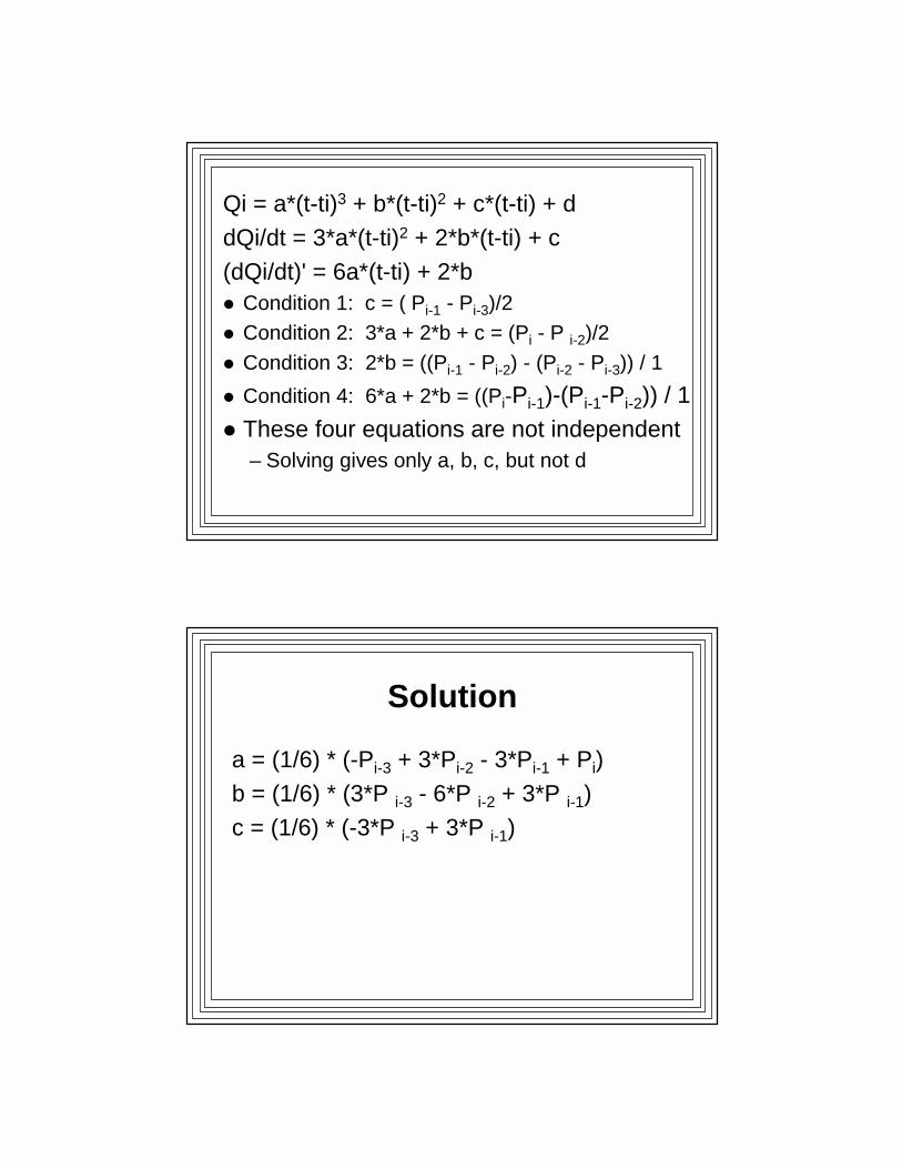
Qi = a*(t-ti)3 + b*(t-ti)2 + c*(t-ti) + ddQi/dt = 3*a*(t-ti)2 + 2*b*(t-ti) + c(dQi/dt)' = 6a*(t-ti) + 2*b� Condition 1: c = ( Pi-1 - Pi-3)/2� Condition 2: 3*a + 2*b + c = (Pi - P i-2)/2� Condition 3: 2*b = ((Pi-1 - Pi-2) - (Pi-2 - Pi-3)) / 1� Condition 4: 6*a + 2*b = ((Pi-Pi-1)-(Pi-1-Pi-2)) / 1� These four equations are not independent

– Solving gives only a, b, c, but not d

Solution

a = (1/6) * (-Pi-3 + 3*Pi-2 - 3*Pi-1 + Pi)b = (1/6) * (3*P i-3 - 6*P i-2 + 3*P i-1)c = (1/6) * (-3*P i-3 + 3*P i-1)

Need another condition to get d� Choose the following condition:

Q (at t=ti) = (1/6) * (P i-3 + 4*P i-2 + P i-1)– i.e., control point at ti (Pi-2) pulls 4 times as hard at t=ti

as control points on either side of ti� Substitute in polynomial equation -->

d = (1/6) * (P i-3 + 4*P i-2 + P i-1)

Uniform Cubic B-Spline Coefficient Matrix Equation

_ _ _ _ _ _| a | |-1 3 -3 1 | | Pi-3 |

| b | = (1/6)*| 3 -6 3 0 | * | Pi-2 |

| c | |-3 0 3 0 | | Pi-1 |

|_d_| |_1 4 1 0_| |_Pi _|

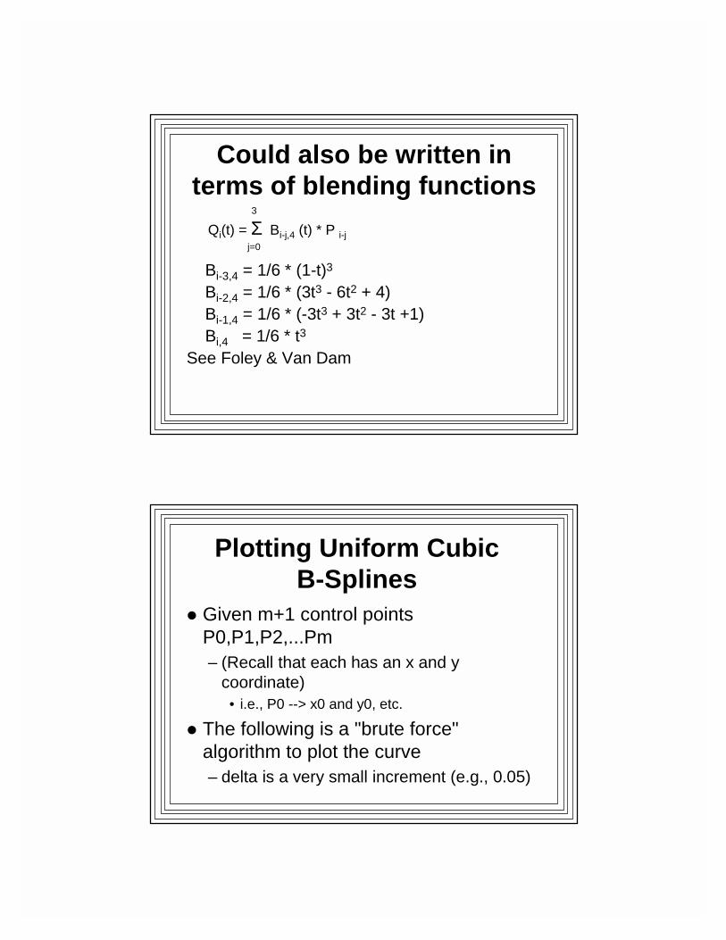
Could also be written in terms of blending functions

3

Qi(t) = Σ Bi-j,4 (t) * P i-jj=0

Bi-3,4 = 1/6 * (1-t)3

Bi-2,4 = 1/6 * (3t3 - 6t2 + 4)Bi-1,4 = 1/6 * (-3t3 + 3t2 - 3t +1)Bi,4 = 1/6 * t3

See Foley & Van Dam

Plotting Uniform Cubic B-Splines

� Given m+1 control points P0,P1,P2,...Pm– (Recall that each has an x and y

coordinate)• i.e., P0 --> x0 and y0, etc.

� The following is a "brute force" algorithm to plot the curve– delta is a very small increment (e.g., 0.05)

For (i=3 to m)Compute ax,bx,cx,dx and ay,by,cy,dy

from control points i-3, i-2, i-1, iFor (t=0; t<=1; t+=delta)

x = ax*t3 + bx*t2 + cx*t + dxy = ay*t3 + by*t2 + cy*t + dyIf (t==0)

MoveTo(x,y)Else

LineTo(x,y)

Brute Force Algorithm

� To increase performance, use forward differences

Closed Cubic B-SplinesMake last 3 control points coincide with 1st 3

0 <--> m-2, 1 <--> m-1, 2 <--> mExample: m=6

Forcing Interpolation

� Reproduce a control point three times� Curve will then go through that point

Properties of Uniform B-Splines

1. Local Control– Each segment determined by only 4 control points

2. Approximates control points; doesn’t interpolate(However it will interpolate triplicated control points)

3. Lies inside convex hull of control points– Each segment lies inside convex hull of its 4 control points

4. Invariant under affine transformations5. Very smooth

– Level-2 continuity everywhere

6. More computations required than for "equivalent" Bezier curve

Bezier vs. B-Spline Curves

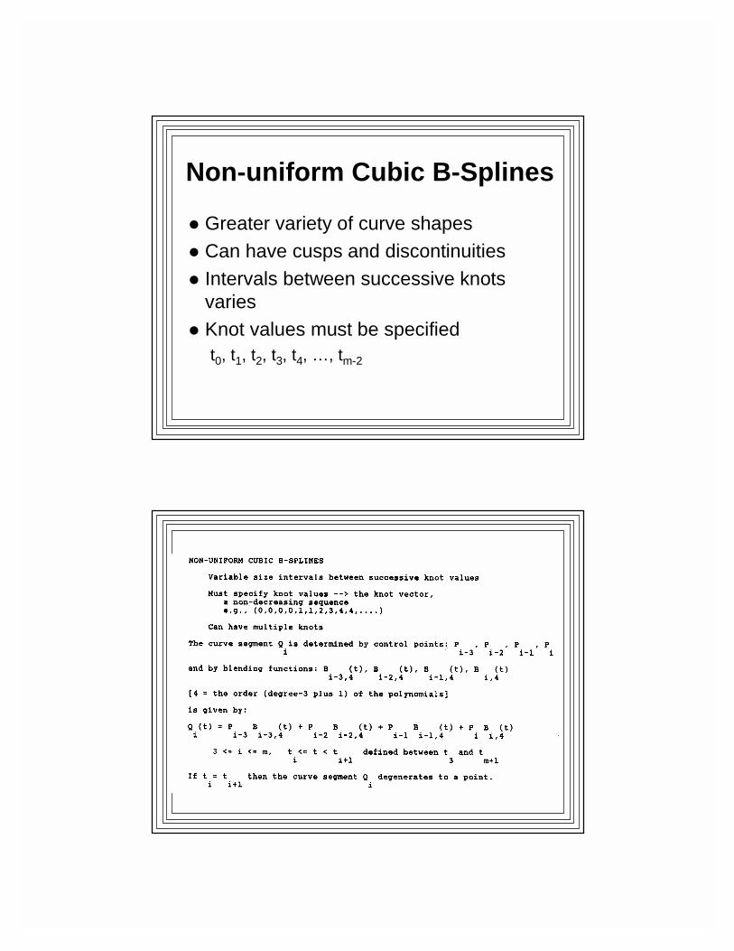
Non-uniform Cubic B-Splines

� Greater variety of curve shapes� Can have cusps and discontinuities� Intervals between successive knots

varies� Knot values must be specified

t0, t1, t2, t3, t4, …, tm-2

Case A (Level-2 Continuity)

� Knot vector: (0,1,2,3,4,5,...)– Just our friend the uniform B-spline

� Q3 determined by P0, P1, P2, P3� Q4 determined by P1, P2, P3, P4� Q3 and Q4 share control points

P1,P2,P3– Three constraints ==> L0, L1, L2 continuity

Case A (Level-2 Continuity)

Case B (Level-1 Continuity)� Knot vector: (0,1,1,2,3,4,...)� Segment Q4 becomes a point

– (since t4 = t5)� Q3 determined by P0, P1, P2, P3� Q5 determined by P2, P3, P4, P5� So Q4 must lie on line connecting P2 & P3� Q3 and Q5 share control points P2 & P3

– Two constraints ==> L0, L1 continuity

Case B (Level-1 Continuity)

Case C (Level-0 continuity)� Knot vector: (0,1,1,1,2,3,...)� Q4 and Q5 become points

– (since t4=t5=t6)� Q3 determined by P0, P1, P2, P3� Q6 determined by P3, P4, P5, P6� So Q4/Q5 must lie on control Point P3

– (interpolates it)� Q3 and Q6 share control point P3

– One constraint ==> L0 continuity

Case C (Level-0 continuity)

Case D (No Continuity-Gaps)� Knot vector: (0,1,1,1,1,2,...)� Q4, Q5, Q6 become points

– (since t4=t5=t6=t7)� Q3 determined by P0, P1, P2, P3� Q7 determined by P4, P5, P6, P7� There is no overlap� Q3 and Q7 share no control points

– No constraints ==> discontinuity

Case D (No Continuity)

3-D Graphics

Overview of 3-D Computer Graphics

� Display image of real or imagined 3-D scene on a 2-D screen

� Modeling and Rendering� Polygon Mesh Models� Bicubic Patch Models� Solid Models

Introduction to 3-D Graphics

Problem # 1: Modeling

� Representing objects in 3-D space� First need to represent points� Use a 3-D coordinate system, e.g.:

– Cartesian: (x, y, z)– Spherical: (rho, theta, phi)– Cylindrical: (r, theta, z)

Conversions� Spherical to Cartesian

x = ρ * sin(φ) * cos(θ)y = ρ * sin(φ) * sin(θ)z = ρ * cos(φ)

RH Coord SystemCould be LH

Viewing system

Types of 3-D Models

� 1. Boundary Representation (B-Rep)– Surface descriptions– Two common ones:

• A. Polygonal• B. Bicubic parametric surface patches

� 2. Solid Representation– Solid modeling

Polygonal Models� Object surfaces approximated by a

mesh of planar polygonsScene -->

Objects -->Sub-objects -->

Polygons -->Vertices (points)

Polygon Mesh Model Example Scene

Bicubic Parametric Surface Patches

� Objects represented by nets of elements called surface patches– Polynomials in two parametric variables– Usually cubic

• Bezier surface patches• B-Spline surface patches

Bicubic Parametric Surface Patches

Solid Representation--Solid Modeling

� Objects represented exactly by combinations of elementary solid objects– e.g., spheres, cylinders, boxes, etc– Called geometric primitives

Constructive Solid Geometry (CSG)

� Complex objects built up by combining geometric primitives using Boolean set operations– union, intersection, difference

� and linear transformations� Object stored as a tree

– Leaves contain primitives– Nodes store set operators or transformations