ba 452 lesson b.4 binary fixed costs 11readingsreadings chapter 7 integer linear programming
TRANSCRIPT

BA 452 Lesson B.4 Binary Fixed Costs 11
Readings
Readings
Chapter 7Integer Linear Programming
BA 452 Lesson B.4 Binary Fixed Costs 22
Overview
Overview

BA 452 Lesson B.4 Binary Fixed Costs 33
Overview
Fixed Costs of Production are those production costs that are present whenever production is positive. The simplest model of fixed costs in a linear program restricts decision variables to binary (0 or 1).
Fixed Costs of Assignment are modeled like Fixed Costs of Production. The simplest model of fixed costs restricts decision variables (the fraction of work completed) to be binary.
Location Covering Problems are a special kind of Linear Programming problem when outputs are fixed because the firm has only established customers, who require coverage by service centers.
Worker Covering Problems are like Location Covering Problems, where customers require scheduling workers so that at each time period is covered by a prescribed minimal number of workers.
Transportation Problems with New Origins are Transportation Problems extended so that new origins may be added, at a fixed cost. They choose the best plant locations and how much to ship.
Transshipment Problems with New Nodes are Transshipment Problems extended so that new transshipment nodes may be added, at a fixed cost. They choose the best transshipment locations.
BA 452 Lesson B.4 Binary Fixed Costs 44
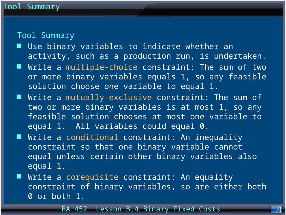
Tool Summary Use binary variables to indicate whether an activity, such as a
production run, is undertaken. Write a multiple-choice constraint: The sum of two or more binary
variables equals 1, so any feasible solution choose one variable to equal 1.
Write a mutually-exclusive constraint: The sum of two or more binary variables is at most 1, so any feasible solution chooses at most one variable to equal 1. All variables could equal 0.
Write a conditional constraint: An inequality constraint so that one binary variable cannot equal unless certain other binary variables also equal 1.
Write a corequisite constraint: An equality constraint of binary variables, so are either both 0 or both 1.
Tool Summary

BA 452 Lesson B.4 Binary Fixed Costs 55
Fixed Cost of Production
Fixed Cost of Production
BA 452 Lesson B.4 Binary Fixed Costs 66
Overview
Fixed Costs of Production are those production costs that are present whenever production is positive. The simplest way to model fixed costs in a linear program is to restrict decision variables to be binary (0 or 1).
For example, suppose the cost of producing quantity x is 5x. On the one hand, if x can take on any non-negative value (like x is the pounds of hamburger produced), then 5 is the constant unit cost of production. On the other hand, if x can take on only binary values (like x is the number of new books adopted), then cost is 0 if there is no production and 5 if there is positive production, so 5 is the fixed cost of production.
Fixed Cost of Production
BA 452 Lesson B.4 Binary Fixed Costs 77
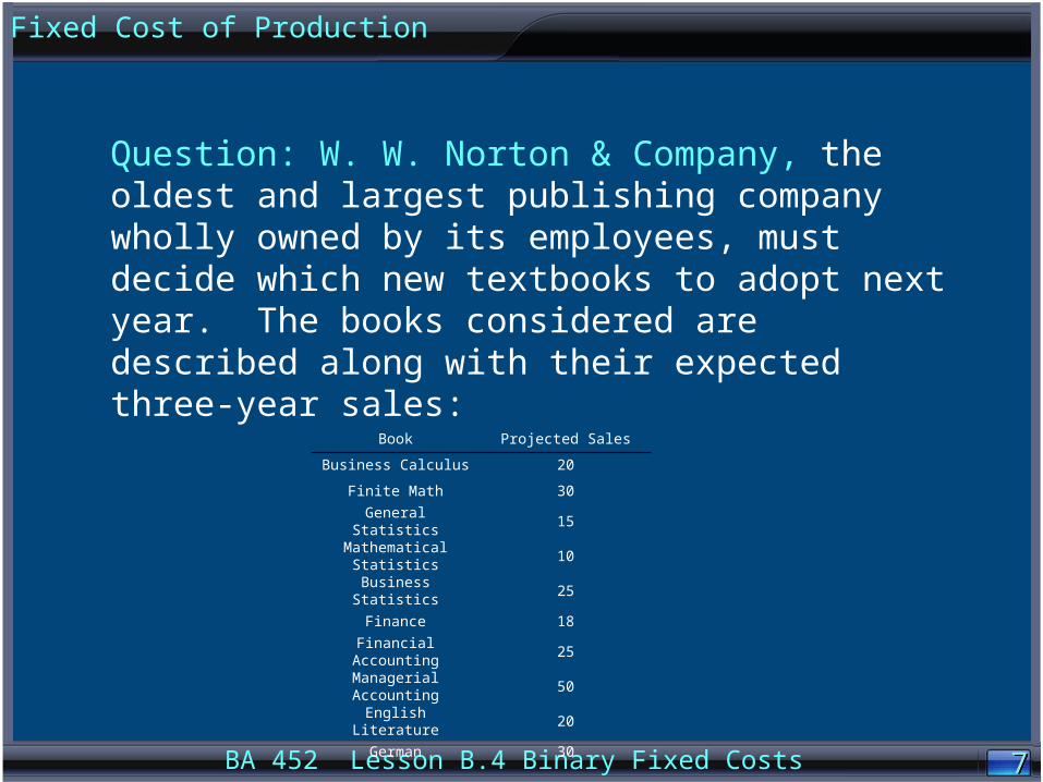
Question: W. W. Norton & Company, the oldest and largest publishing company wholly owned by its employees, must decide which new textbooks to adopt next year. The books considered are described along with their expected three-year sales:
Fixed Cost of Production
Book Projected Sales
Business Calculus 20
Finite Math 30
General Statistics 15
Mathematical Statistics 10
Business Statistics 25
Finance 18
Financial Accounting 25
Managerial Accounting 50
English Literature 20
German 30

BA 452 Lesson B.4 Binary Fixed Costs 88
Three individuals in the company can be assigned to these projects, all of whom have varying amounts of time available. John has 60 days, Susan has 52 days, and Monica has 43 days. The days required by each person to complete each project are showing in the following table. For example, if the business calculus book is published, it will require 30 days of John’s time and 40 days of Susan’s time.
Book Projected Sales John Susan Monica
Business Calculus 20 30 40 X
Finite Math 30 16 24 X
General Statistics 15 24 X 30
Mathematical Statistics 10 20 X 24
Business Statistics 25 10 X 16
Finance 18 X X 14
Financial Accounting 25 X 24 26
Managerial Accounting 50 X 28 30
English Literature 20 40 34 30
German 30 x 50 36
Fixed Cost of Production

BA 452 Lesson B.4 Binary Fixed Costs 99
Norton will not publish more than two statistics books or more than one accounting book in a single year. In addition, one of the math books (business calculus or finite math) must be published, but not both. Which books should be published, and what are the projected sales? If Monica has 1 more day available, which books should be published, and what are the projected sales? Comment.
Fixed Cost of Production

BA 452 Lesson B.4 Binary Fixed Costs 1010
xi =1 if book i is scheduled for publication0 otherwise{Let
i Book
1 Business Calculus
2 Finite Math
3 General Statistics
4 Mathematical Statistics
5 Business Statistics
6 Finance
7 Financial Accounting
8 Managerial Accounting
9 English Literature
10 German
Fixed Cost of Production

BA 452 Lesson B.4 Binary Fixed Costs 1111
Max 20x1 + 30x2 + 15x3 + 10x4 + 25x5 + 18x6 + 25x7 + 50x8 + 20x9 + 30x10s.t.
30x1 + 16x2 + 24x3 + 20x4 + 10x5 + 40x9 £ 60 John40x1 + 24x2 + 24x7 + 28x8 + 34x9 + 50x10 £ 52 Susan
30x3 + 24x4 + 16x5 + 14x6 + 26x7 + 30x8 + 30x9 + 36x10 £ 43 Monicax3 + x4 + x5 £ 2 No. of Stat Books
x7 + x8 £ 1 Account Bookx1 + x2 = 1 Math Book
i Book Projected Sales John Susan Monica
1 Business Calculus 20 30 40 X
2 Finite Math 30 16 24 X
3 General Statistics 15 24 X 30
4 Mathematical Statistics 10 20 X 24
5 Business Statistics 25 10 X 16
6 Finance 18 X X 14
7 Financial Accounting 25 X 24 26
8 Managerial Accounting 50 X 28 30
9 English Literature 20 40 34 30
10 German 30 x 50 36
Fixed Cost of Production
BA 452 Lesson B.4 Binary Fixed Costs 1212
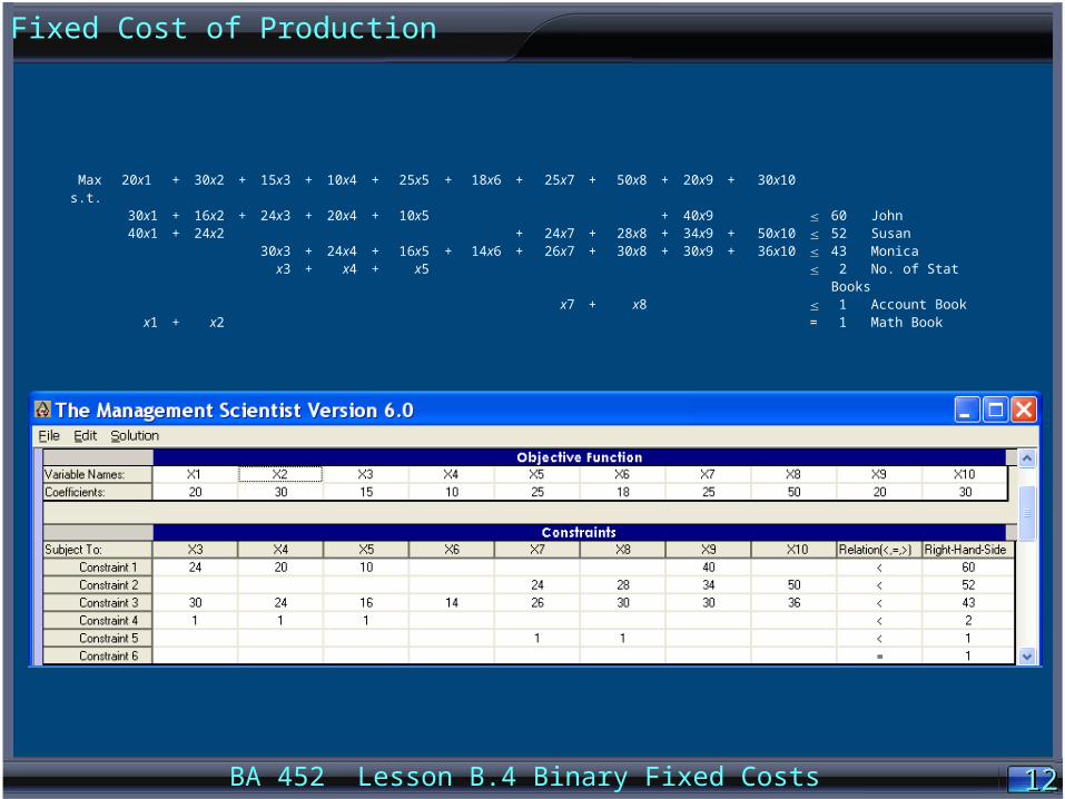
Max 20x1 + 30x2 + 15x3 + 10x4 + 25x5 + 18x6 + 25x7 + 50x8 + 20x9 + 30x10s.t.
30x1 + 16x2 + 24x3 + 20x4 + 10x5 + 40x9 £ 60 John40x1 + 24x2 + 24x7 + 28x8 + 34x9 + 50x10 £ 52 Susan
30x3 + 24x4 + 16x5 + 14x6 + 26x7 + 30x8 + 30x9 + 36x10 £ 43 Monicax3 + x4 + x5 £ 2 No. of Stat Books
x7 + x8 £ 1 Account Bookx1 + x2 = 1 Math Book
Fixed Cost of Production
BA 452 Lesson B.4 Binary Fixed Costs 1313
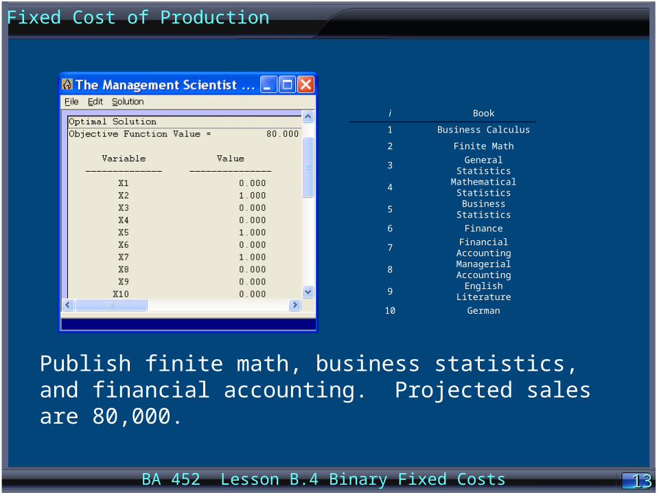
Publish finite math, business statistics, and financial accounting. Projected sales are 80,000.
i Book
1 Business Calculus
2 Finite Math
3 General Statistics
4 Mathematical Statistics
5 Business Statistics
6 Finance
7 Financial Accounting
8 Managerial Accounting
9 English Literature
10 German
Fixed Cost of Production

BA 452 Lesson B.4 Binary Fixed Costs 1414
Publish finite math, business statistics, and financial accounting. Projected sales are 80,000.
i Book
1 Business Calculus
2 Finite Math
3 General Statistics
4 Mathematical Statistics
5 Business Statistics
6 Finance
7 Financial Accounting
8 Managerial Accounting
9 English Literature
10 German
Fixed Cost of Production
BA 452 Lesson B.4 Binary Fixed Costs 1515
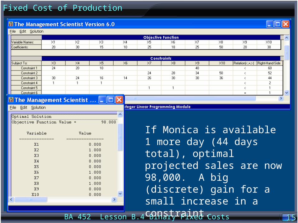
If Monica is available 1 more day (44 days total), optimal projected sales are now 98,000. A big (discrete) gain for a small increase in a constraint.
Fixed Cost of Production

BA 452 Lesson B.4 Binary Fixed Costs 1616
Fixed Cost of Assignment
Fixed Cost of Assignment

BA 452 Lesson B.4 Binary Fixed Costs 1717
Overview
Fixed Costs of Assignment are modeled like Fixed Costs of Production. The simplest model of fixed costs restricts decision variables to be binary.
For example, suppose the cost of worker i performing the fraction xij of job j is 5xij. On the one hand, if xij can take on any non-negative value between 0 and 1 (like xij is the fraction of the job performed), then 5 is the constant unit cost of assignment (like the time cost of working). On the other hand, if xij can take on only binary values, then cost is 0 if you are not assigned (xij = 0) and 5 if you are assigned the entire job (xij = 1), so 5 is the fixed cost of assignment (like the cost of commuting to a job across town).
Fixed Cost of Assignment

BA 452 Lesson B.4 Binary Fixed Costs 1818
Question: Tina's Tailoring has five idle tailors and four custom garments to make. The estimated time (in hours) it would take each tailor to make each garment is shown in the next slide. (An 'X' in the table indicates an unacceptable tailor-garment assignment.)
Tailor
Garment 1 2 3 4 5 Wedding gown 19 23 20 21 18
Clown costume 11 14 X 12 10 Admiral's uniform 12 8 11 X 9 Bullfighter's outfit X 20 20 18 21
Fixed Cost of Assignment
BA 452 Lesson B.4 Binary Fixed Costs 1919
Formulate an integer program for determining the tailor-garment assignments that minimize the total estimated time spent making the four garments. No tailor is to be assigned more than one garment, and each garment is to be worked on by only one tailor.
This particular problem can be formulated as either a binary program or as an integer program. Any feasible solution to the latter program is binary (0-1).
Fixed Cost of Assignment

BA 452 Lesson B.4 Binary Fixed Costs 2020
Answer: Define the decision variables
= 1 if garment i is assigned to tailor j
= 0 otherwise. Find the number of decision variables
= [(number of garments)x(number of tailors)]
- (number of unacceptable assignments)
= [4x5] - 3 = 17 Find the number of constraints. 1 for each garment and each tailor = 9.
xij
Fixed Cost of Assignment
BA 452 Lesson B.4 Binary Fixed Costs 2121
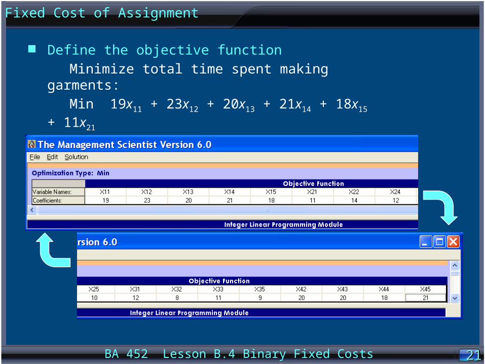
Define the objective function
Minimize total time spent making garments:
Min 19x11 + 23x12 + 20x13 + 21x14 + 18x15 + 11x21
+ 14x22 + 12x24 + 10x25 + 12x31 + 8x32 + 11x33
+ 9x35 + 20x42 + 20x43 + 18x44 + 21x45
Fixed Cost of Assignment
BA 452 Lesson B.4 Binary Fixed Costs 2222
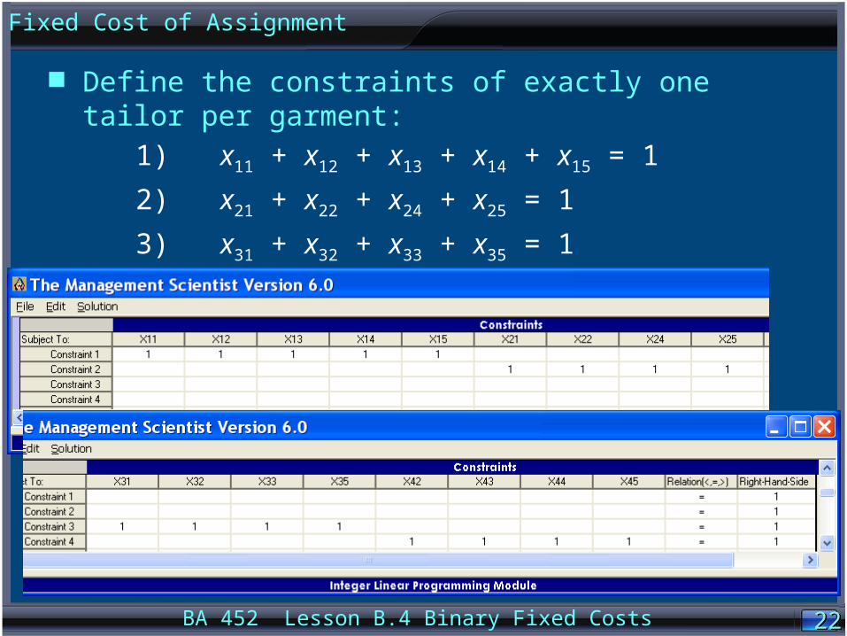
Define the constraints of exactly one tailor per garment:
1) x11 + x12 + x13 + x14 + x15 = 1
2) x21 + x22 + x24 + x25 = 1
3) x31 + x32 + x33 + x35 = 1
4) x42 + x43 + x44 + x45 = 1
Fixed Cost of Assignment
BA 452 Lesson B.4 Binary Fixed Costs 2323
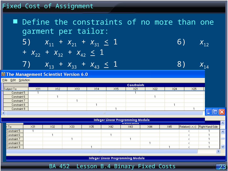
Define the constraints of no more than one garment per tailor:
5) x11 + x21 + x31 < 1 6) x12 + x22 + x32 + x42 < 1
7) x13 + x33 + x43 < 1 8) x14 + x24 + x44 < 1
9) x15 + x25 + x35 + x45 < 1
Fixed Cost of Assignment

BA 452 Lesson B.4 Binary Fixed Costs 2424
Tailor
Garment 1 2 3 4 5 Wedding gown 19 23 20 21 18
Clown costume 11 14 X 12 10 Admiral's uniform 12 8 11 X 9 Bullfighter's outfit X 20 20 18 21
Minimum time: 55 hoursOptimal assignments:
Fixed Cost of Assignment

BA 452 Lesson B.4 Binary Fixed Costs 2525
Location Covering
Location Covering
BA 452 Lesson B.4 Binary Fixed Costs 2626
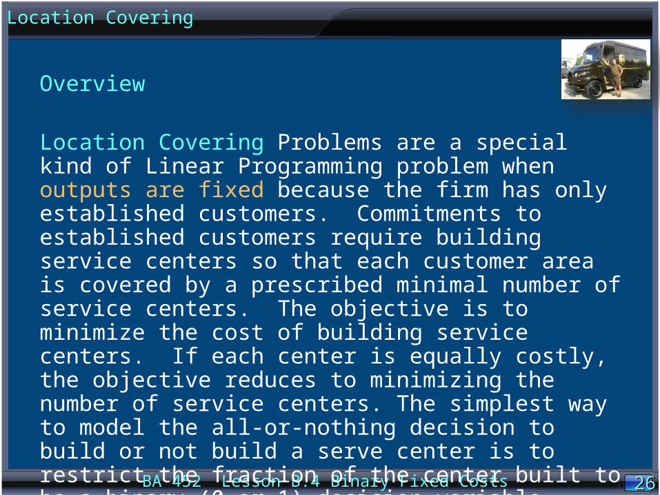
Overview
Location Covering Problems are a special kind of Linear Programming problem when outputs are fixed because the firm has only established customers. Commitments to established customers require building service centers so that each customer area is covered by a prescribed minimal number of service centers. The objective is to minimize the cost of building service centers. If each center is equally costly, the objective reduces to minimizing the number of service centers. The simplest way to model the all-or-nothing decision to build or not build a serve center is to restrict the fraction of the center built to be a binary (0 or 1) decision variable.
Location Covering
BA 452 Lesson B.4 Binary Fixed Costs 2727
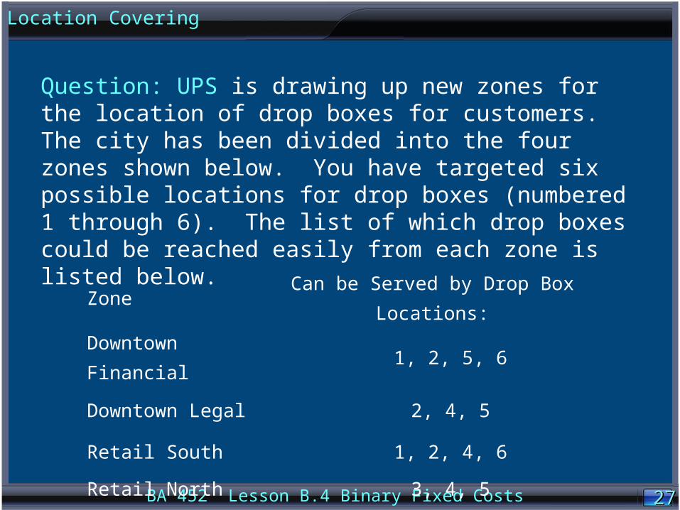
Question: UPS is drawing up new zones for the location of drop boxes for customers. The city has been divided into the four zones shown below. You have targeted six possible locations for drop boxes (numbered 1 through 6). The list of which drop boxes could be reached easily from each zone is listed below.
Zone Can be Served by Drop Box Locations:
Downtown Financial
1, 2, 5, 6
Downtown Legal 2, 4, 5
Retail South 1, 2, 4, 6
Retail North 3, 4, 5
Location Covering

BA 452 Lesson B.4 Binary Fixed Costs 2828
Formulate and solve a model to provide the fewest drop-box locations yet make sure that each zone is covered by at least two boxes.
Location Covering
BA 452 Lesson B.4 Binary Fixed Costs 2929
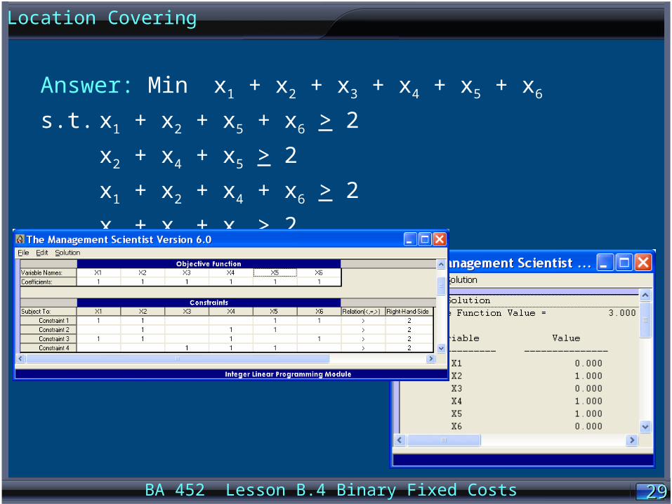
Answer: Min x1 + x2 + x3 + x4 + x5 + x6
s.t. x1 + x2 + x5 + x6 > 2
x2 + x4 + x5 > 2
x1 + x2 + x4 + x6 > 2
x3 + x4 + x5 > 2
Location Covering

BA 452 Lesson B.4 Binary Fixed Costs 3030
Worker Covering
Worker Covering

BA 452 Lesson B.4 Binary Fixed Costs 3131
Overview
Worker Covering Problems are like Location Covering Problems. Outputs are fixed because the firm has only established customers. Commitments to established customers require scheduling workers so that at each time period customer needs are covered by a prescribed minimal number of workers. The objective is to minimize the cost of scheduling workers. If each worker is equally costly, the objective reduces to minimizing the number of workers scheduled. The simplest way to model the all-or-nothing decision to schedule a worker is to restrict the number of workers scheduled at each time period to be an integer decision variable.
Worker Covering
BA 452 Lesson B.4 Binary Fixed Costs 3232
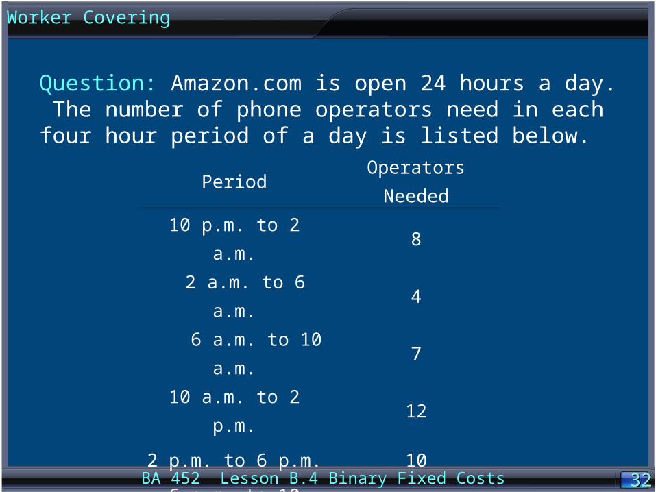
Question: Amazon.com is open 24 hours a day. The number of phone operators need in each four hour period of a day is listed below.
Period Operators Needed
10 p.m. to 2 a.m. 8
2 a.m. to 6 a.m. 4
6 a.m. to 10 a.m. 7
10 a.m. to 2 p.m. 12
2 p.m. to 6 p.m. 10
6 p.m. to 10 p.m. 15
Worker Covering

BA 452 Lesson B.4 Binary Fixed Costs 3333
Suppose operators work for eight consecutive hours.
Formulate and solve the company’s problem of determining how many operators should be scheduled to begin working in each period in order to minimize the number of cashiers needed? (Hint: Workers can work from 6 p.m. to 2 a.m.)
Worker Covering

BA 452 Lesson B.4 Binary Fixed Costs 3434
Answer: Define the decision variables
TNP = the number of operators who begin working at 10 p.m.
TWA = the number of operators who begin working at 2 a.m.
SXA = the number of operators who begin working at 6 a.m.
TNA = the number of operators who begin working at 10 a.m.
TWP = the number of operators who begin working at 2 p.m.
SXP = the number of operators who begin working at 6 p.m.
Min TNP + TWA + SXA + TNA + TWP + SXP
s.t.TNP + TWA > 4
TWA + SXA > 7
SXA + TNA > 12
TNA + TWP > 10
TWP + SXP > 15
SXP + TNP > 8, all variables > 0
Worker Covering

BA 452 Lesson B.4 Binary Fixed Costs 3535
Worker Covering
BA 452 Lesson B.4 Binary Fixed Costs 3636
Transportation with New Origins
Transportation with New Origins

BA 452 Lesson B.4 Binary Fixed Costs 3737
Transportation Problems with New Origins are Transportation Problems extended so that new origins may be added, at a fixed cost. Also called Distribution System Design Problems, they choose the best plant locations and determine how much to ship from each plant. The simplest way to model those fixed costs in a linear program is with binary (0 or 1) variables.
For example, consider a Transportation Problem extended by allowing the possibility of developing a new origin. Suppose the fixed development cost is 5 and the new origin’s supply capacity is 7. That is a linear program with a supply of 7Y at the new origin and added cost term of 5Y, where Y = 0 indicates the new origin is not developed and Y = 1 indicates the new origin is developed.
Transportation with New Origins
BA 452 Lesson B.4 Binary Fixed Costs 3838
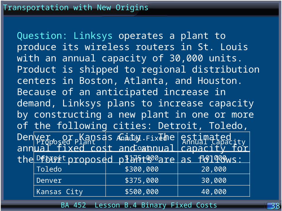
Question: Linksys operates a plant to produce its wireless routers in St. Louis with an annual capacity of 30,000 units. Product is shipped to regional distribution centers in Boston, Atlanta, and Houston. Because of an anticipated increase in demand, Linksys plans to increase capacity by constructing a new plant in one or more of the following cities: Detroit, Toledo, Denver, or Kansas City. The estimated annual fixed cost and annual capacity for the four proposed plants are as follows:
Proposed Plant Annual Fixed Cost Annual Capacity
Detroit $175,000 10,000
Toledo $300,000 20,000
Denver $375,000 30,000
Kansas City $500,000 40,000
Transportation with New Origins

BA 452 Lesson B.4 Binary Fixed Costs 3939
The company’s long-range planning group forecasts of the anticipated annual demand at the distribution centers are as follows:
Distribution Center Annual Demand
Boston 30,000
Atlanta 20,000
Houston 20,000
Transportation with New Origins
BA 452 Lesson B.4 Binary Fixed Costs 4040
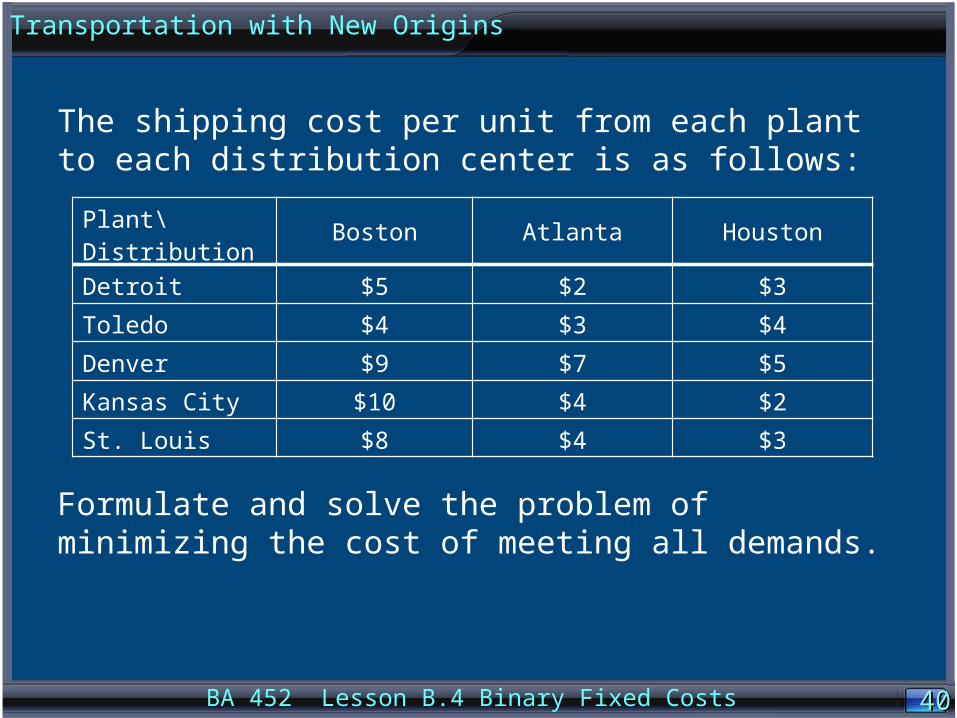
The shipping cost per unit from each plant to each distribution center is as follows:
Formulate and solve the problem of minimizing the cost of meeting all demands.
Plant\Distribution Boston Atlanta Houston
Detroit $5 $2 $3
Toledo $4 $3 $4
Denver $9 $7 $5
Kansas City $10 $4 $2
St. Louis $8 $4 $3
Transportation with New Origins

BA 452 Lesson B.4 Binary Fixed Costs 4141
Answer: Define binary variables for plant construction,Y1 = 1 if a plan is constructed in Detroit; 0, if notY2 = 1 if a plan is constructed in Toledo; 0, if notY3 = 1 if a plan is constructed in Denver; 0, if notY4 = 1 if a plan is constructed in Kansas City; 0, if not
Define shipment variables just as in transportation problems,Xij = the units shipped (in thousands) from plant i (i = 1, 2, 3, 4, 5) to distribution center j (j = 1, 2, 3) each year.
Transportation with New Origins

BA 452 Lesson B.4 Binary Fixed Costs 4242
The objective is minimize total cost.
From cost data
shipping costs (in thousands of dollars) are5X11 + 2X12 + 3X13+ 4X21 + 3X22 + 4X23 + 9X31 + 7X32 + 5X33 + 10X41 + 4X42 + 2X43 + 8X51 + 4X52 + 3X53
Plant\Distribution Boston Atlanta Houston
Detroit $5 $2 $3
Toledo $4 $3 $4
Denver $9 $7 $5
Kansas City $10 $4 $2
St. Louis $8 $4 $3
Transportation with New Origins

BA 452 Lesson B.4 Binary Fixed Costs 4343
From cost data
plant construction costs (in thousands of dollars) are175Y1 + 300Y2 + 375Y3 + 500Y4
Hence, the objective to minimize total costs isMin 5X11 + 2X12 + 3X13+ 4X21 + 3X22 + 4X23 + 9X31 + 7X32 + 5X33 + 10X41 + 4X42 + 2X43 + 8X51 + 4X52 + 3X53 + 175Y1 + 300Y2 + 375Y3 + 500Y4
Proposed Plant Annual Fixed Cost Annual Capacity
Detroit $175,000 10,000
Toledo $300,000 20,000
Denver $375,000 30,000
Kansas City $500,000 40,000
Transportation with New Origins
BA 452 Lesson B.4 Binary Fixed Costs 4444
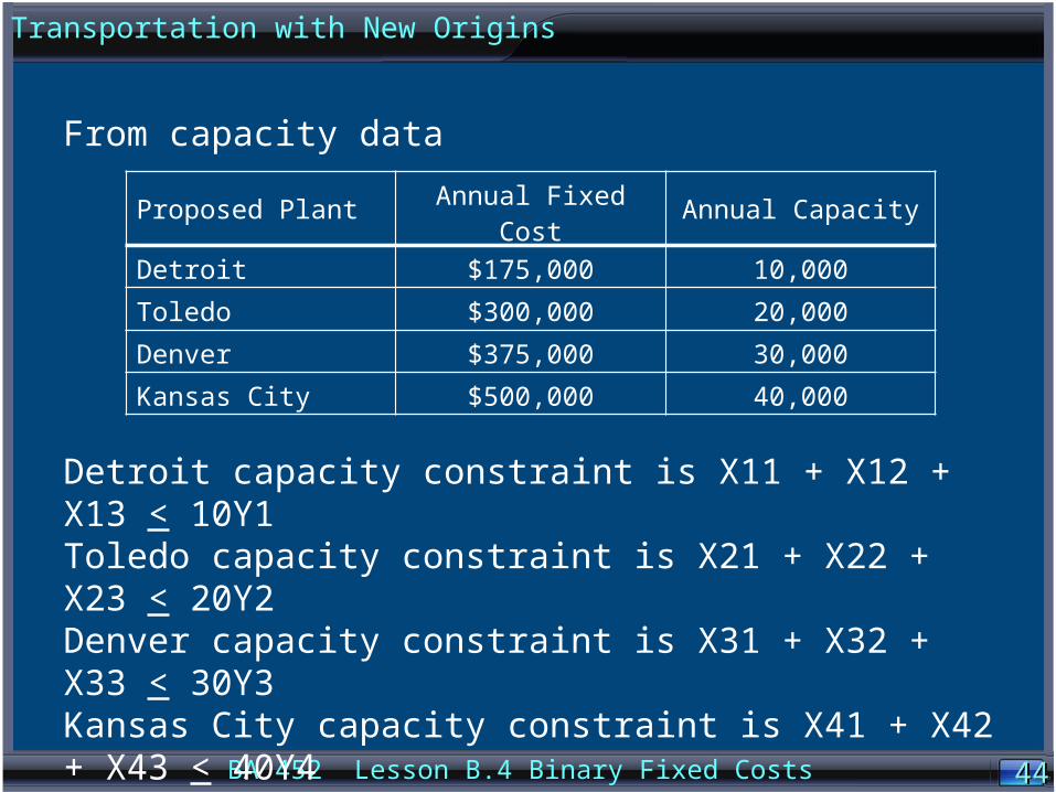
From capacity data
Detroit capacity constraint is X11 + X12 + X13 < 10Y1Toledo capacity constraint is X21 + X22 + X23 < 20Y2Denver capacity constraint is X31 + X32 + X33 < 30Y3Kansas City capacity constraint is X41 + X42 + X43 < 40Y4
And St. Louis capacity constraint is X51 + X52 + X53 < 30
Proposed Plant Annual Fixed Cost Annual Capacity
Detroit $175,000 10,000
Toledo $300,000 20,000
Denver $375,000 30,000
Kansas City $500,000 40,000
Transportation with New Origins
BA 452 Lesson B.4 Binary Fixed Costs 4545
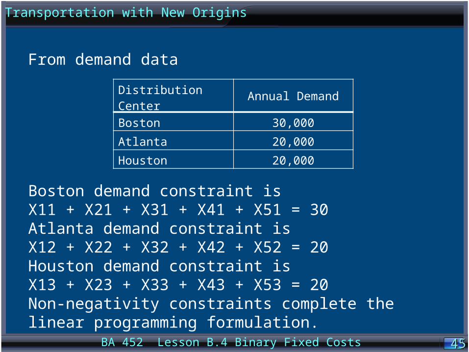
From demand data
Boston demand constraint isX11 + X21 + X31 + X41 + X51 = 30Atlanta demand constraint isX12 + X22 + X32 + X42 + X52 = 20Houston demand constraint isX13 + X23 + X33 + X43 + X53 = 20Non-negativity constraints complete the linear programming formulation.
Distribution Center Annual Demand
Boston 30,000
Atlanta 20,000
Houston 20,000
Transportation with New Origins

BA 452 Lesson B.4 Binary Fixed Costs 4646
From demand data
Boston demand constraint isX11 + X21 + X31 + X41 + X51 = 30Atlanta demand constraint isX12 + X22 + X32 + X42 + X52 = 20Houston demand constraint isX13 + X23 + X33 + X43 + X53 = 20Non-negativity constraints complete the linear programming formulation.
Distribution Center Annual Demand
Boston 30,000
Atlanta 20,000
Houston 20,000
Transportation with New Origins
BA 452 Lesson B.4 Binary Fixed Costs 4747
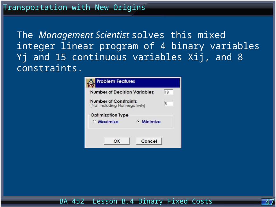
The Management Scientist solves this mixed integer linear program of 4 binary variables Yj and 15 continuous variables Xij, and 8 constraints.
Transportation with New Origins

BA 452 Lesson B.4 Binary Fixed Costs 4848
Transportation with New Origins

BA 452 Lesson B.4 Binary Fixed Costs 4949
The Management Scientist solves this mixed integer linear program of 4 binary variables Yj and 15 continuous variables Xij, and 8 constraints.
Transportation with New Origins

BA 452 Lesson B.4 Binary Fixed Costs 5050
All variables at the optimum are zero except: X42 = 20, X43 = 20, X51 = 30, and Y4 = 1.
So, the Kansas City plant should be built; 20,000 units should be shipped from Kansas City to Atlanta; 20,000 units should be shipped from Kansas City to Houston; and 30,000 units should be shipped from St. Louis to Boston.
Transportation with New Origins

BA 452 Lesson B.4 Binary Fixed Costs 5151
Transshipment with New Nodes
Transshipment with New Nodes

BA 452 Lesson B.4 Binary Fixed Costs 5252
Overview
Transshipment Problems with New Transshipment Nodes are Transshipment Problems extended so that new transshipment nodes may be added, at a fixed cost. They choose the best transshipment locations and determine how much to ship through each location. The simplest way to model those fixed costs in a linear program is with binary (0 or 1) variables.
Transshipment with New Nodes

BA 452 Lesson B.4 Binary Fixed Costs 5353
Question: Zeron Industries supplies three firms (Zrox, Hewes, Rockrite) with customized shelving for its offices. Zeron orders shelving from the same two manufacturers, Arnold Manufacturers and Supershelf, Inc. Currently, weekly demands by the users are 50 for Zrox, 60 for Hewes, and 40 for Rockrite. Both Arnold and Supershelf can supply up to 75 units to its customers.
Zeron currently ships from its Northside facilities, but it can develop Southside facilities for a fixed cost of 8. Unit costs from the manufacturers to the suppliers are:
Zeron N Zeron S Arnold 5 8 Supershelf 7 4
The costs to install the shelving at the various locations are:
Zrox Hewes Rockrite Zeron N 1 5 8
Zeron S 3 4 4
Transshipment with New Nodes

BA 452 Lesson B.4 Binary Fixed Costs 5454
ARNOLD
WASHBURN
HEWES
75
75
50
60
40
5
8
7
4
15
8
3
44
Arnold
SuperShelf
Hewes
Zrox
ZeronN
ZeronS
Rock-Rite
Transshipment with New Nodes

BA 452 Lesson B.4 Binary Fixed Costs 5555
Define decision variables:
xij = amount shipped from manufacturer i to supplier j
xjk = amount shipped from supplier j to customer k
where i = 1 (Arnold), 2 (Supershelf)
j = 3 (Zeron N), 4 (Zeron S)
k = 5 (Zrox), 6 (Hewes), 7 (Rockrite)
y = 1 if Zeron S is developed, y = 0 if Zeron S is not developed
Transshipment with New Nodes
BA 452 Lesson B.4 Binary Fixed Costs 5656
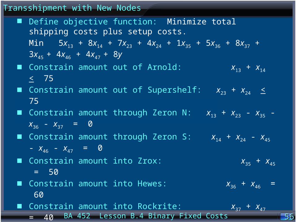
Define objective function: Minimize total shipping costs plus setup costs.
Min 5x13 + 8x14 + 7x23 + 4x24 + 1x35 + 5x36 + 8x37 + 3x45 + 4x46 + 4x47
+ 8y Constrain amount out of Arnold: x13 + x14 < 75
Constrain amount out of Supershelf: x23 + x24 < 75
Constrain amount through Zeron N: x13 + x23 - x35 - x36 - x37 = 0
Constrain amount through Zeron S: x14 + x24 - x45 - x46 - x47 = 0
Constrain amount into Zrox: x35 + x45 = 50
Constrain amount into Hewes: x36 + x46 = 60
Constrain amount into Rockrite: x37 + x47 = 40
Setup indicator for Zeron S: x45 + x46 + x47 < 150y
(The first 4 constraints imply x45 + x46 + x47 < 150, so the setup indicator constraint “x45 + x46 + x47 < 150y” means, at an optimum, y = 1 if any material x45 or x46 or x47 transships through Zeron S, and y = 0 if no material x45 or x46 or x47 transships through Zeron S.)
Transshipment with New Nodes

BA 452 Lesson B.4 Binary Fixed Costs 5757
BA 452 Quantitative Analysis
End of Lesson B.4