bachelor of engineering thesis - espace.library.uq.edu.au415809/campos_rojas... · this project...
TRANSCRIPT

THE UNIVERSITY OF QUEENSLAND
Bachelor of Engineering Thesis
Feasibility of Using a Conveyor Based System of Stripping at the Wombat
Project
Student Name: Giselle Campos Rojas
Course Code: MINE 4123
Academic Supervisor: Adjunct Professor Warren Seib
Industry Supervisor: James Cooney
Submission Date: 7 November 2016
A thesis submitted in partial fulfilment of the
requirements of the Bachelor of Engineering degree in
Mining Engineering
UQ Engineering
Faculty of Engineering, Architecture and Information Technology

STATEMENT OF ORIGINALITY
I hereby declare that this thesis research project report is my own work and that it contains, to
the best of my knowledge and belief, no material previously published or written work by
another person nor material which to a substantial extent has been submitted for another course,
except where due acknowledgement is made in the report.
Signed,
Giselle Campos Rojas

ACKNOWLEDGEMENTS
This project would not have been completed without the support from others. This is why I
would like thank New Hope Group for making this project available to develop my thesis. I
would also like to express my greatest gratitude to Warren Seib, my academic supervisor, for
providing me the opportunity to work on this project and for his guidance. To James Cooney,
my industry supervisor, for his constant support and guidance, his valuable feedback and
mentoring through this project. I appreciate his help in working through the challenges I faced
and the models for comparison, and for taking the time to explain what I needed to learn for
this project. I feel truly privileged to have worked with him. I would also like to thank the
industry representatives for providing part of the data I needed to build the models. Especially
to Stefan Blunck from RWE for his generosity in sharing his vast experience in continuous
mining as well as proposing alternatives to improve the project, and to Adrian Rokovic, from
Thyssen Krupp, for taking the time out of his busy schedule to provide the information for the
IPCC system. Finally to Paul Hoogwerf, my partner, for his patience and unconditional support
throughout my degree.

i
ABSTRACT
This project investigated the use of a continuous mining system to strip overburden at the
greenfield Wombat deposit at a concept level. This project will develop an open cut thermal
coal mine in the Surat Basin. The project was analysed using truck and shovel in 2013 and a
dragline in 2015, but due to market conditions, it was not found economically feasible.
In this study, a bucket wheel excavator (BWE) and an in-pit crushing and conveying (IPCC)
system were evaluated. The geotechnical analysis showed that free-digging with a BWE was
not guaranteed, therefore the study focused on a fully mobile IPCC at a 5 Mtpa production rate.
The aim was to reduce operating costs and improve the economic feasibility of the project in
current conditions. The key objectives were to determine the technical and economic viability
of an IPCC system and develop a financial model to compare it with the 2013 and 2015 studies.
A block model in Minescape software was input in XPAC software to create a schedule at a
target production rate of 5 Mtpa. The XPAC output was exported to Excel to build a financial
model. Three models were initially created which were compared with the 2015 dragline case:
IPCC with a large rope shovel.
IPCC with a smaller face shovel.
Truck and excavator case (TEX) as a baseline for comparison.
The models yielded 30 years life of mine and 150 Mt reserves. It was found that a realistic
comparison with the 2015 dragline model was not possible, and a revised dragline model was
built. A coal price of USD69.2/t was used and the project was not found economically feasible,
although the revised dragline case produced the most favourable results, with smallest negative
net present value (NPV) of around -AUD1.8b.
Financing the IPCC infrastructure was also investigated. This improved the IPCC results,
however the revised dragline still performed better than both IPCC and TEX (2 to 8% better).
The rope shovel proved the best option for loading the IPCC.
Finally, an assessment was done at a coal price of USD120/t which enabled a comparison with
the 2013 truck and shovel case. This revealed that the new models improved the financial results

ii
due to an increased mine life and larger reserves. Again the revised dragline case yielded the
best results, highest NPV and IRR as shown in Table i. The TEX, however had better results
than both IPCC models because of the lower break-even coal price with TEX. The rope shovel
was also found to be better for loading the IPCC than the hydraulic face shovel.
Table i. NPV and IRR results at USD120/t
Case IPCC Face Shovel
Financed IPCC Rope
Shovel Financed TEX
Revised Dragline
T&S
NPV (AUDm) 420 432 454 515 95
IRR (%) 16% 16% 16% 17% 12%
In spite of the dragline producing the best results, the other scenarios were close, within a ±30%
variance as expected from a concept study. Thus, it was found that more research and further
assessment are needed to arrive to a definite conclusion since all results were drawn at a concept
level. The risks related to each alternative mining method also must be analysed.
It is also recommended to analyse the IPCC models at a higher production rate, investigate
different financing options for IPCC infrastructure, compare the cost of overburden removal
only between each method, and research the optimisation of the interburden removal.

iii
CONTENTS
Abstract ........................................................................................................................................ i
Introduction .......................................................................................................................... 1
1.1 Background .................................................................................................................. 1
1.2 Problem Definition ...................................................................................................... 1
1.3 Aims and Objectives .................................................................................................... 2
1.4 Scope ............................................................................................................................ 3
1.4.1 Scope Inclusions ..................................................................................................... 3
1.4.2 Scope Exclusions .................................................................................................... 3
1.5 Project Significance ..................................................................................................... 4
1.5.1 Relevance to Industry ............................................................................................. 4
1.5.2 Knowledge Gap ...................................................................................................... 4
1.6 Assumptions ................................................................................................................. 4
1.7 Constraints ................................................................................................................... 5
1.8 Methodology ................................................................................................................ 5
1.8.1 Research.................................................................................................................. 5
1.8.2 Analysis .................................................................................................................. 5
1.8.3 Results .................................................................................................................... 6
1.9 Project Management .................................................................................................... 6
1.9.1 Project Stakeholders ............................................................................................... 6
1.9.2 Project Deliverables ................................................................................................ 7
1.9.3 Project Schedule ..................................................................................................... 7
1.9.4 Project Delivery Risk Assessment .......................................................................... 7
Overview of the Wombat Project ........................................................................................ 9
2.1 Project Location ........................................................................................................... 9
2.1.1 Geology .................................................................................................................. 9
2.2 Existing Mine Plan ..................................................................................................... 11
2.2.1 Existing Environmental Impact Statement ........................................................... 12
2.3 Previous Investigation ................................................................................................ 12
2.4 Current Thermal Coal Market Conditions ................................................................. 13
Strip Mining and Equipment .............................................................................................. 14
3.1 Commonly Used Equipment in Coal Strip Mining ................................................... 16
3.2 BWE and IPCC Systems ............................................................................................ 18

iv
3.2.1 BWE ..................................................................................................................... 18
3.2.2 Types of BWE ...................................................................................................... 19
3.2.3 BWE Implementation ........................................................................................... 19
3.2.4 BWE Productivity ................................................................................................ 21
3.2.5 BWE Selection ..................................................................................................... 21
3.2.6 IPCC ..................................................................................................................... 22
3.2.7 Types of IPCC ...................................................................................................... 23
3.2.8 IPCC Implementation ........................................................................................... 24
3.2.9 IPCC Productivity ................................................................................................ 27
3.2.10 IPCC Selection ..................................................................................................... 28
3.2.11 Advantages and disadvantages of IPCC systems ................................................. 28
3.3 Application of BWE and IPCC Systems to Surface Mining ..................................... 29
3.3.1 Continuous Mining Systems ................................................................................. 30
3.4 Technical Requirements to Implement BWE and IPCC Systems ............................. 30
Geotechnical Conditions Assessment ................................................................................ 32
4.1 Geological setting ...................................................................................................... 32
4.2 Groundwater .............................................................................................................. 33
4.3 Geotechnical Assessment .......................................................................................... 34
4.4 Stripping Horizons at the Wombat Project ................................................................ 35
4.5 Infrastructure Requirements ...................................................................................... 38
4.5.1 IPCC Equipment Selection ................................................................................... 38
4.5.2 IPCC System Working Method ............................................................................ 39
Models ............................................................................................................................... 41
5.1 XPAC Models ............................................................................................................ 41
5.1.1 Reserves Modelling .............................................................................................. 41
5.2 Excel Models ............................................................................................................. 44
5.2.1 Production Schedule ............................................................................................. 44
5.2.2 Primary Equipment Productivity .......................................................................... 46
5.2.3 Ancillary Equipment ............................................................................................ 47
5.2.4 Hauling Equipment ............................................................................................... 48
5.2.5 Other Equipment .................................................................................................. 48
5.2.6 Capital and Replacement Schedule ...................................................................... 49
5.2.7 Personnel .............................................................................................................. 50
5.2.8 Rehabilitation Costs .............................................................................................. 51
v
5.2.9 Operating Costs .................................................................................................... 51
5.2.10 Financial Model .................................................................................................... 51
Results ................................................................................................................................ 53
6.1 Preliminary Results .................................................................................................... 53
6.1.1 Methodology Summary ........................................................................................ 53
6.1.2 Infrastructure Capital and Equipment Costs Results ............................................ 54
6.1.3 Personnel Results .................................................................................................. 54
6.1.4 Operating Costs Results ....................................................................................... 55
6.1.5 Break-Even Coal Price ......................................................................................... 55
6.1.6 Financial Model Results ....................................................................................... 56
6.1.7 Preliminary Results Comparison .......................................................................... 56
6.2 Updated Results ......................................................................................................... 59
6.2.1 Revised Dragline Model Results .......................................................................... 60
6.2.2 Sensitivity Analysis .............................................................................................. 63
6.2.3 Financing Options for IPCC Infrastructure .......................................................... 67
6.3 Results at USD120/t ................................................................................................... 69
6.4 Project Risks .............................................................................................................. 70
6.4.1 Operational Risks ................................................................................................. 71
6.4.2 Financial Risks ..................................................................................................... 72
6.4.3 Environmental and Social Risks ........................................................................... 72
6.4.4 Health and Safety Risks ........................................................................................ 72
Conclusions ........................................................................................................................ 73
Recommendations .............................................................................................................. 75
References .......................................................................................................................... 76
Appendix 1: Project Management ............................................................................................ 81
Project Management Plan ......................................................................................................... 81
Project Schedule ................................................................................................................ 81
Project Milestones .............................................................................................................. 81
Project Related Resources ................................................................................................. 82
Project Related Budget ...................................................................................................... 82
Project Delivery Risk Assessment ..................................................................................... 82
Appendix 2: Existing Minescape Plots and XPAC Schedule .................................................. 87
Appendix 3: Geology & Geotechnical Data ............................................................................. 90
Appendix 4: XPAC Plots .......................................................................................................... 95

vi
Appendix 5: Balanced Mining Schedules ................................................................................ 99
Appendix 6: Time Usage Model ............................................................................................ 101
Appendix 7: Personnel and Rehabilitation Assumptions ....................................................... 102
Appendix 8: Excavator and Truck Units ................................................................................ 104

vii
LIST OF TABLES
Table 1. Project risk assessment post-controls. ......................................................................... 8
Table 2. Wombat Project reserves modelling assumptions ...................................................... 11
Table 3. Comparison between shovel, dragline and BWE ....................................................... 17
Table 4. Comparison between IPCC options ........................................................................... 24
Table 5. Summary of standing water levels at the Wombat lease ............................................ 33
Table 6. Summary of UCS results from 2008 and 2009 .......................................................... 34
Table 7. IPCC Equipment requirements ................................................................................... 39
Table 8. Primary equipment allocated to each material and pit ............................................... 45
Table 9. Productivity assumptions for primary equipment ...................................................... 47
Table 10. Ancillary equipment included in the analysis .......................................................... 48
Table 11. IPCC face shovel infrastructure capital and depreciable life assumptions ............... 49
Table 12. Equipment life and rebuild time assumptions .......................................................... 50
Table 13. Summary of operating costs ..................................................................................... 51
Table 14. Infrastructure and equipment capital costs ............................................................... 54
Table 15. Personnel numbers and annual cost .......................................................................... 55
Table 16. Preliminary results percent change comparison with TEX ...................................... 57
Table 17. Updated infrastructure and equipment capital costs ................................................. 60
Table 18. Updated personnel numbers and annual cost ........................................................... 60
Table 19. Percent change comparison with TEX for updated results ...................................... 62
Table 20. Percent change results for financed IPCC infrastructure ......................................... 68
Table 21. NPV and IRR results at USD120/t ........................................................................... 70

viii
LIST OF FIGURES
Figure 1. Queensland's Coal Systems Map and Relative Location of the Wombat Project .... 10
Figure 2. Thermal coal price in AUD/t from April 2011 to March 2016. ................................ 13
Figure 3. Typical strip mining process. .................................................................................... 14
Figure 4. Conveyor based mining system ............................................................................... 15
Figure 5. Compact BWE . ........................................................................................................ 18
Figure 6. Block digging a lateral terrace cut with BWE .......................................................... 19
Figure 7. Bench and lateral block excavation with BWE......................................................... 20
Figure 8. Cross pit spreading with transverse conveyor bridge. .............................................. 20
Figure 9. Cross pit spreading with mobile spreader. ................................................................ 20
Figure 10. Waste spreader. ....................................................................................................... 22
Figure 11. Semi-mobile crusher at the Mae Moh mine ............................................................ 22
Figure 12. Example of fully mobile in-pit crushing. ................................................................ 23
Figure 13. IPCC haul road example. ........................................................................................ 25
Figure 14. Semi-mobile crusher station designed in the wall................................................... 26
Figure 15. Semi-mobile crusher station accessed through a temporary ramp .......................... 26
Figure 16. Semi-mobile crusher station accessed from the haul road ...................................... 27
Figure 17. Stratigraphical cross-section at the Wombat Project .............................................. 33
Figure 18. Topography at the Wombat Project. ....................................................................... 36
Figure 19. Overburden thickness at the Wombat Project. ........................................................ 37
Figure 20. Coal thickness at the Wombat Project. ................................................................... 38
Figure 21. IPCC conceptual layout........................................................................................... 39
Figure 22. Proposed IPCC system ........................................................................................... 40
Figure 23. Pipe layer arrangement . .......................................................................................... 40
Figure 24. Maximum cash flow positive XPAC plot for IPCC. .............................................. 43
Figure 25. Raw waste volumes from XPAC for both Pits. ...................................................... 45
Figure 26. Simplified methodology model. .............................................................................. 53
Figure 27. Operating costs comparison at 5 Mtpa. ................................................................... 55
Figure 28. Break-even coal price at 5 Mtpa. ............................................................................ 56
Figure 29. Financial models preliminary results. ..................................................................... 56
Figure 30. Preliminary results percent change comparison with TEX. .................................... 57
Figure 31. Comparison of waste volume across all cases. ....................................................... 58
Figure 32. Comparison of coal tonnage across all cases. ......................................................... 58

ix
Figure 33. Waste volume comparison for the Wombat Deposit. ............................................. 59
Figure 34. Revised methodology model. .................................................................................. 60
Figure 35. Updated operating costs comparison at 5 Mtpa. ..................................................... 61
Figure 36. Fixed operating costs. ............................................................................................. 61
Figure 37. Updated break-even coal price. ............................................................................... 62
Figure 38. Updated financial model results. ............................................................................. 62
Figure 39. Updated results percent change comparison with TEX. ......................................... 63
Figure 40. Sensitivity analysis IPCC face shovel. .................................................................... 64
Figure 41. Sensitivity analysis IPCC rope shovel. ................................................................... 64
Figure 42. Sensitivity analysis TEX. ........................................................................................ 65
Figure 43. Sensitivity analysis revised dragline. ...................................................................... 65
Figure 44. Sensitivity comparison capital costs. ...................................................................... 66
Figure 45. Sensitivity comparison labour costs. ....................................................................... 66
Figure 46. Comparison of labour requirements. ....................................................................... 67
Figure 47. Sensitivity comparison electricity. .......................................................................... 67
Figure 48. Comparison of financed IPCC models. ................................................................... 68
Figure 49. Financed IPCC and dragline results compared to TEX. ......................................... 69
Figure 50. NPV and IRR comparison at 120 USD/t................................................................. 70
Figure 51. SWOT for IPCC risks. ............................................................................................ 74

1
INTRODUCTION
1.1 BACKGROUND
The Wombat Project entails the development of an open cut thermal coal mine within the Surat
Basin. The lease is located around 35 km west of the Township of Wandoan in the Darling
Downs region in Southern Queensland (NHG, 2013). This is a greenfield project (NHG, 2015),
based on a previous proposal to mine 8.2 Mtpa Run of Mine (ROM) coal for export. Horse
Creek crosses the Mining Lease Application (MLA) from north to south and the previous
proposal included the diversion of this creek (NHG, 2013).
New Hope Group (NHG) is an Australian owned and operated Energy Company (NHG, 2016)
which holds total control over the MLA (NHG, 2015). In 2013, NHG conducted an internal
review of the previous proposal and margin ranked the deposit to develop a new plan to exploit
only economically viable reserves. Six different mine planning scenarios were examined,
including the preservation and diversion of Horse Creek. A cut-off stripping ratio was also
imposed (NHG, 2013).
This analysis showed that the diverted creek scenarios were economically attractive at a
production rate of 5 or 7 Mtpa using traditional truck and shovel operation (NHG, 2013) with
a mine life of 17 years (NHG, 2015). The reportable reserves within the positive margin areas
indicated Total Coal Reserves of 125.2 Mt ROM coal within the lease (NHG, 2015).
1.2 PROBLEM DEFINITION
In 2011, a Feasibility Study was done to develop the Wombat Project using truck and shovel
operation. This was followed by the 2013 internal review using the same method. At the time,
it was concluded that the project was not economically viable as a standalone option. The main
limitations were the lack of established transport infrastructure for product coal from pit to port,
the sustained decline in coal price and the variability of the exchange rate (Wilson, 2015).
Alternative mining methods were then evaluated to assess the feasibility of the project in current
market conditions. In 2014, a study investigated the use of a surface miner, while in 2015 a
second study assessed the use of a surface miner in conjunction with a dragline and bulk dozer

2
push for overburden stripping. These studies concluded that further research was needed to
establish the economic viability of the Wombat Project (Uren, 2014 and Wilson, 2015).
At present, NHG is considering the development of the project as part of a portfolio of other
interests the Company holds in the region, with the aim of overcoming the project’s limitations.
The current strategy is to assess the feasibility of each of the projects in the portfolio and then
integrate them onto a major project base (Cooney, 2016).
It was anticipated that a continuous mining system with either a Bucket Wheel Excavator
(BWE) or In-pit crushing and conveying (IPCC) would improve the Net Present Value (NPV)
of the project by reducing operating costs over the life of mine (LOM) (Cooney, 2016). The
present study investigated the viability of implementing a continuous mining system as an
alternative to the previously investigated overburden stripping methods.
1.3 AIMS AND OBJECTIVES
The aim of this project was to assess the feasibility of implementing a continuous mining system
for overburden removal at the Wombat Project, and to compare this option with previously
evaluated alternatives. To achieve this aim, several specific objectives were defined.
Review the studies from 2014 and 2015 that investigated different overburden stripping
methods. This provided relevant background information for the current study.
Review current information for the Wombat Project, relevant to the present study,
including but not limited to:
- existing mine plan;
- geological and geotechnical information;
- environmental impact statement (EIS);
- thermal coal market conditions; and
- NHG’s present strategy to develop the project.
Determine suitable stripping horizons and lithology for strip mining. This enabled a
preliminary selection of a BWE or IPCC.
Investigate previous applications of BWE and IPCC systems in the mining industry and
establish the technical requirements for their implementation. This provided a better
understanding of how these systems operate.

3
Assess the technical feasibility of implementing a continuous mining system and
develop a mining schedule. This established if the option was feasible.
Develop a financial model to assess the economic feasibility of using a continuous
mining system. This enabled a comparison.
Compare the results of the financial model for the continuous mining system with the
methods previously investigated and determine the optimal exploitation method for the
deposit. This enabled a decision on whether a continuous mining method would improve
the performance of the project in current conditions.
Provide conclusions on the assessment and recommendations. This fulfilled the
project’s aim.
1.4 SCOPE
The present study focused on current conditions to develop the Wombat Project and the
implementation of either a BWE or IPCC system.
1.4.1 Scope Inclusions
The scope of the project included:
Reviewing the current project conditions and project documentation;
Examining the geology and geotechnical variables within the mining lease;
Identifying the advantages and disadvantages of BWE and IPCC systems; and
Identifying the risks of implementing a BWE or IPCC systems to develop the project.
1.4.2 Scope Exclusions
Items that lay beyond the scope of the project were:
Identifying and assessing a suitable exploitation method should the proposed BWE or
IPCC system be rendered unviable;
Investigating options to finance the BWE or IPCC system; and
Updating relevant project documentation for approval such as the MLA or EIS if the
BWE or IPCC system were found attractive for the development of the project.

4
1.5 PROJECT SIGNIFICANCE
1.5.1 Relevance to Industry
The Wombat Project MLA is one of several other applications within the South East
Queensland region (Queensland Government, 2016). The success of this and other projects
relies on the access to the required infrastructure. If such infrastructure were to be built it would
not only guarantee the development of the Wombat deposit but also of the Surat Basin as a new
coal basin in Queensland (NHG, 2015) as well as other resources such as the Galilee Basin.
This development would ensure sustained income for state and federal governments. It would
also provide job security for people directly employed in mining operations with the potential
to expand employment opportunities in related services. The transport infrastructure needed for
mining projects may also contribute to the development of other industries such as farming, by
providing alternative transport options for their products.
1.5.2 Knowledge Gap
Although continuous mining systems offer several benefits, these methods are not commonly
used in Australian mines. Continuous mining systems are used in Victoria to mine brown coal
with BWEs, but these methods have not been used extensively in Queensland. There are only
a couple of mines in Queensland that have partially implemented a continuous method, one
using a BWE (Cooney, 2016c) and another one with in-pit crushing (Blunck, 2016). Using a
continuous mining system would help narrow the knowledge gap concerning the application of
these methods in Queensland coal mines.
1.6 ASSUMPTIONS
Assumptions that were made to deliver this project include:
NHG has 100% ownership of the land where the MLA is based;
The diversion of Horse Creek has been approved within the MLA;
The Wombat Project has been granted approval for development by relevant authorities
including provision of a licence to operate; and
The construction of the transport infrastructure to the port depends on a consortium of
third parties and such expenditure will not affect the present study.

5
1.7 CONSTRAINTS
Based on current information and assumptions, these constraints restricted the execution of this
project:
Existing mining lease boundaries;
Requirements enforced by the EIS as defined for the approved MLA;
Conditions that led to the approval of the licence to operate;
Current Company financial structure and thermal coal market conditions;
Access to infrastructure required to implement the proposed system; and
Legal requirements as set out in the Coal Mining Safety and Health Act (1999) and the
Queensland Coal Mining Safety and Health Regulation (2001).
1.8 METHODOLOGY
To complete this research project, the methodology used consisted of three main stages.
1.8.1 Research
Literature review of existing project documentation, application of BWE and IPCC systems,
technical requirements for implementing each system and potential stripping horizons.
1.8.2 Analysis
Technical and economic feasibility of implementing a BWE or IPCC system. This involved
assessing the geological and geotechnical conditions, infrastructure requirements, developing
mine sequences and a proposed layout. To assess the economic feasibility of a BWE or IPCC
system, the steps shown below were followed (Cooney, 2016a) which required the use of
specialised software, namely Minescape and XPAC.
1. A block model of topography, interburden, overburden and coal was created in
Minescape.
2. The Minescape model was input into XPAC to develop a schedule to mine the blocks.
XPAC is a scheduling software package that produced volume of waste and tonnage of
coal to be moved by each type of equipment to achieve a target of production.

6
3. The results from XPAC were exported into an Excel spreadsheet to create a mining
schedule and determine the equipment needed to complete the mining sequence.
4. A financial model was created in Excel to carry out the economic evaluation.
1.8.3 Results
A baseline was established for comparison, to integrate results from the present and previous
studies. This consisted of an Excel spreadsheet based on the common XPAC output outlined in
step 3 in the analysis (Section 1.8.2). It must be noted that the results drawn in this research
were targeted at a concept level study and not a full feasibility assessment.
1.9 PROJECT MANAGEMENT
To ensure the project was completed in time and to the highest quality, a project management
plan was defined where key stakeholders and project deliverables were outlined. The plan
included a schedule of activities and project milestones, project related resources, a budget, an
assessment of the risks that threatened the completion of the project as well as a contingency
plan. The project had an estimated budget of AUD17 120 as outlined in Appendix 1.
This contingency plan came into effect when one of the computers used to develop the project,
stopped working and the backup data was retrieved to complete project delivery. The project
management plan is detailed in Appendix 1 while the following subsections summarise the key
aspects of project delivery.
1.9.1 Project Stakeholders
The key stakeholders for the delivery of this project were:
Project Manager: A Mining Engineering student accountable for ensuring the project
tasks were completed and project objectives were achieved within the set timeframe.
Client: A NHG representative that oversaw the technical aspects of the project (industry
supervisor).
Project Sponsor: An academic who supervised and provided guidance in completing the
agreed objectives, assisted in negotiating any changes in the project scope and provided
feedback based on defined criteria.

7
1.9.2 Project Deliverables
At the completion of the project, the key deliverables will be:
A written document that includes the background of the work done and findings. This
will constitute a bachelor of engineering thesis.
A set of Minescape plots generated for the project.
A set of XPAC plots, scripts and reports generated for the project.
A set of Excel spreadsheets created for each scenario assessed.
A research paper.
1.9.3 Project Schedule
This research project was delivered over the course of two university semesters. As mentioned,
the project schedule can be found in Appendix 1. The project started on 7 March 2016, and it
had a duration of 160 days. It was completed on 7 November 2016.
1.9.4 Project Delivery Risk Assessment
Risk management is a key element of project management. Identifying potential threats to
project delivery and implementing a contingency plan assisted in ensuring the project was on
track and reached completion. For this project, the Contingency Plan shown in Table 1 was
created to reduce the identified risks to as low as reasonably possible (Moderate or Low). This
Contingency Plan was based on controls defined after identifying and assessing the risks that
affected project delivery as outlined in Appendix 1.

8
Table 1.
Project risk assessment post-controls.
Hazard
Pre-Control
Risk Rank Control
Post-Control
Risk Rank
Traffic delays / transport problems
High (H) Ensure transport routes are planned and
sufficient time for travel is factored in Identify alternative transport arrangements
Low (L)
Data inaccessible or insufficient
High (H)
Identify required information and ensure past data is readily available
Identify information gaps and devise a plan with stakeholders to work around available data
Moderate (M)
Data corruption or loss Extreme
(E) Backup data to local drive, USB or Cloud Email to self a copy of updated/new files Low (L)
Breach of confidentiality
Extreme (E)
Change project name prior to saving files and only save to a secure location (password encrypted USB)
Moderate (M)
Industry supervisor unavailability
High (H)
Define planned times of absence (e.g. annual leave) and plan accordingly
Identify key go to person if industry supervisor is unavailable longer than anticipated
Schedule regular meetings and set targets for each session in line with the project plan
Ensure contact details are up to date (landline, mobile and email)
Low (L)
University supervisor unavailability
High (H) Arrange key meeting times well in advance Low (L)
Lost time due to sickness or Illness
Extreme (E)
Ensure work-life balance Immediately inform supervisors if repeated
or sustained period of illness (e.g. over a week) and re-assess project.
Keep ahead of key due dates
Moderate (M)
Project submitted to lower than desirable quality
Extreme (E)
Complete tasks as per project criteria and check quality prior to submission
Initiate project early and allow ample time for quality assurance
Low (L)
Unable to submit finalised Project
Extreme (E)
Track project progress and re-schedule as needed
Initiate project early to allow ample slack Submission deadline is confirmed
Low (L)

9
OVERVIEW OF THE WOMBAT PROJECT
The scope of the Wombat Project is to develop a thermal coal resource in the order of 250 Mt.
The project has evolved from a Feasibility Study completed in 2011 and a Project Evaluation
Study in 2012. A mine plan was also developed by a consulting group, which aimed at
maximising the mineable reserves within the lease boundaries. An Environmental Impact Study
(EIS) was prepared based on this mine plan. In 2013, NHG carried out an internal review of the
project information and analysed different scenarios to identify mineable reserves only. Margin
ranking of these reserves was also completed (NHG, 2013).
2.1 PROJECT LOCATION
The project is located within the Surat Basin coal province at approximately 35 km west of
Wandoan in the Darling Downs region of Southern Queensland. The Wombat Project depends
on the infrastructure associated with the proposed Surat Basin Railway being constructed
(NHG, 2013). Figure 1 shows a map of Queensland’s coal systems with the town of Wandoan
highlighted by a red circle to show the relative location of the Wombat Project. This figure also
shows the proposed Surat Basin Railway the project relies on.
One of the main features within the mining lease is the presence of Horse Creek that runs across
the mining area and flows from north to south (NHG, 2013). In the original mine plan, different
scenarios were assessed including the creek remains and creek diverted options.
2.1.1 Geology
The Wombat Project is located in the central northern Surat Basin and the coal seams lie within
the Mimosa Syncline axis, which trends north-south. Along this syncline is where the thickest
deposition occurred. The coal seams within the mining lease are from the Juandah Coal
Measures, which lie between the Tangalooma Sandstone and Taroom Coal Measures to form
the Walloon Sub Group (NHG, 2013).
The Wombat Project was modelled considering 40 individual coal seam plys and the seam
groups in decreasing order from the top surface are the UG, Y, A, B, BC, C and LG seams.
These seams are inter-banded with siltstones and mudstones; however, sections of clean, low
ash coal with few stone bands are also present (NHG, 2013).

10
Figure 1. Queensland's Coal Systems Map and Relative Location of the Wombat Project
(Queensland Government, 2010).

11
Several rainbow plots were generated in Minescape using the geological model, to determine
the topography, base of weathering (BOW), overburden and interburden thickness as well as
the areas where the thickest coal exists. These plots are found in Appendix 2, where it can be
seen that the deposit is mostly shallow, with an average depth ranging from 20 to 30 m to top
of coal. Depth increases as topography rises to the south.
The plot of cumulative coal thickness relative to pit boundaries is also included in Appendix 2.
This thickness comprised all the seams in the geological model. It was observed that the thickest
coal areas lie at the centre of the lease, intersecting the location of Horse Creek. This explains
the in-situ ratio plot in Appendix 2, which shows that the lowest stripping ratio concentrates at
the centre of the lease, where Horse Creek is located. The density from the quality model was
used to generate this in-situ ratio plot, and it was considered representative of all coal seams.
Based on this analysis, the mining sequence in 2013 defined the target coal extraction areas at
the centre of the lease.
2.2 EXISTING MINE PLAN
In-situ reserves were generated using the geological model, which were then converted into
mineable reserves using XPAC software. A series of assumptions (outlined in Table 2) were
made to develop the mineable reserves and to margin rank the deposit.
Table 2.
Wombat Project reserves modelling assumptions
Working section dilution (m) 0.025 m on roof and 0.05 m on floor
Working section loss (m) 0 m CHPP efficiency factor 0.94 CHPP dilution removal efficiency 0.94 Min. mineable imported coal thickness (m) 0.10 Min. parting separation thickness (m) 0.15 Dilution ash (%) 81.7 Dilution relative density (g/cc) 2.4 Thin parting/thick parting cut-off (m) 1.5
Source: NHG (2013)
After margin ranking, the break-even in-situ cut-off was established, which defined the pit
boundaries. A cut-off of 6:1 was applied to determine the economic pit boundaries for the truck
and shovel case. It must be emphasised that the existing mine plan will not sterilise any coal
above the 6:1 ratio; thus if economic conditions change the mine can be re-designed accordingly

12
(NHG, 2013). The deposit was divided into four pits: A, B, C and D, and a schedule was
developed using 100 m x 100 m blocks. The schedule for the 5 Mtpa production rate with creek
diversion scenario from 2013 is provided in Appendix 2.
2.2.1 Existing Environmental Impact Statement
An environmental impact statement (EIS) was completed for the Wombat deposit, using an
open cut mining method with truck and shovel. The processing plant was originally designed
to handle up to 8.2 Mtpa ROM coal to achieve a production rate of 5 Mtpa for the 286 Mt
resource. The roster adopted was 24 hours a day and 7 days per week. The LOM was 40 years
including mine closure. This EIS defined the open pit boundaries, specific requirements for
waste dumps, water and power supply, rehabilitation, and cultural heritage (Wilson, 2015).
2.3 PREVIOUS INVESTIGATION
Wilson (2015) carried out a study to assess the feasibility of implementing a dragline for
overburden stripping considering the use of bulk dozer push and surface miners as an integrated
system, and to compare them with the original truck and shovel plan. In this analysis, the dragline
would use cast and extended bench digging to mine overburden and interburden greater than 10 m,
the surface miners would mine the coal and parting horizons, and truck and shovel were assigned
to overburden and interburden less than 10 m thick. Another scenario was assessed in which the
dragline was replaced by a fleet of bulk dozers. The results from this study showed that the most
feasible option was using bulk dozer push for overburden removal to produce 6 Mtpa of coal.
In 2014, Uren completed a study to evaluate the use of a surface miner for overburden stripping
and coal mining at the Wombat Project. This study however, focused on net present costs to
operate this equipment based on site data from other mines that NHG managed. The study
showed that a surface miner could potentially eliminate the need for a crusher at the Coal
Handling and Preparation Plant (CHPP) because of the functionality of the machine. It was also
recommended to investigate the use of a conveyor system in conjunction with the surface miner
to improve operating costs. In discussion with the Client, for the present study it was decided
to only focus on the 2013 truck and shovel results and the 2015 dragline case for comparison.
13
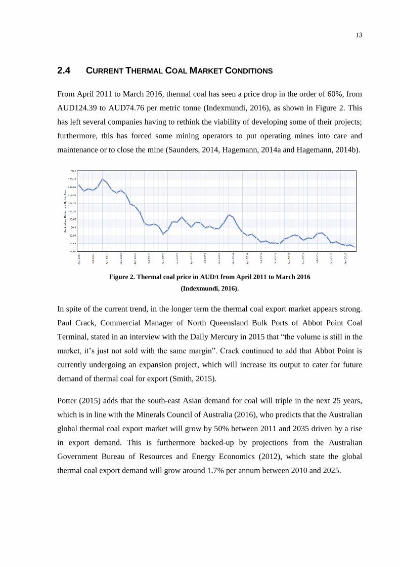
2.4 CURRENT THERMAL COAL MARKET CONDITIONS
From April 2011 to March 2016, thermal coal has seen a price drop in the order of 60%, from
AUD124.39 to AUD74.76 per metric tonne (Indexmundi, 2016), as shown in Figure 2. This
has left several companies having to rethink the viability of developing some of their projects;
furthermore, this has forced some mining operators to put operating mines into care and
maintenance or to close the mine (Saunders, 2014, Hagemann, 2014a and Hagemann, 2014b).
Figure 2. Thermal coal price in AUD/t from April 2011 to March 2016
(Indexmundi, 2016).
In spite of the current trend, in the longer term the thermal coal export market appears strong.
Paul Crack, Commercial Manager of North Queensland Bulk Ports of Abbot Point Coal
Terminal, stated in an interview with the Daily Mercury in 2015 that “the volume is still in the
market, it’s just not sold with the same margin”. Crack continued to add that Abbot Point is
currently undergoing an expansion project, which will increase its output to cater for future
demand of thermal coal for export (Smith, 2015).
Potter (2015) adds that the south-east Asian demand for coal will triple in the next 25 years,
which is in line with the Minerals Council of Australia (2016), who predicts that the Australian
global thermal coal export market will grow by 50% between 2011 and 2035 driven by a rise
in export demand. This is furthermore backed-up by projections from the Australian
Government Bureau of Resources and Energy Economics (2012), which state the global
thermal coal export demand will grow around 1.7% per annum between 2010 and 2025.

14
STRIP MINING AND EQUIPMENT
Strip mining is a surface mining method used to exploit bedded deposits such as coal. The main
difference with open pit mining methods is that the overburden is placed directly on pre-mined
panels (strips) rather than sending this material to a waste dump location (Hartman and
Mutmansky, 2002). The sequence of development for strip mining from initial workings to
mine closure can be summarised into six steps (Dyer and Hill, 2011):
1 Land clearing and topsoil removal.
2 Fragmentation.
3 Removal of waste.
4 Placement of waste including restoration of soil and initial revegetation.
5 Coal mining.
6 Mine restoration, maintenance and eventual closure.
A typical strip mining process is shown in Figure 3.
Figure 3. Typical strip mining process
(Dyer and Hill, 2011).
Hartman and Mutmansky (2002) classify strip mining as a large-scale mining method,
commonly used because of its high productivity and low unit operating cost. In addition, since

15
the overburden is placed in mined-out panels, the mining activity is concentrated to a relatively
small surface and reclamation can be done immediately after mining is complete.
The key to productivity lies on the output of the stripping excavator. This is achieved by using
the largest machines available because they reduce the number of active mining faces. In spite
of this advantage, the method is susceptible to equipment downtime because a single machine
is responsible for all of production. The process of excavating and dumping the material in a
final location is referred to as casting. Normally excavation and casting are carried out with a
single piece of equipment including draglines, BWEs, shovels, trucks, front end loaders and
scrapers, although the overburden can also be loaded onto conveyors for transport to the final
location (Hartman and Mutmansky, 2002). Figure 4 shows a typical schematic layout of a strip
mine setting using conveyor based stripping. Note that the equipment is dedicated to either
mining waste or ore.
Figure 4. Conveyor based mining system
(Cooney, 2015).
In large strip mines, the location of the processing plant must be considered for the given site
conditions, as to minimise the haul distances. This decision may also be influenced by the
surface transport system adopted (Hartman and Mutmansky, 2002).

16
3.1 COMMONLY USED EQUIPMENT IN COAL STRIP MINING
In coal strip mines, mining is normally done using conventional loading and hauling equipment.
Loading and excavation are one of the primary unit operations carried out in any mine, and
several types of equipment are available to perform such operations. The equipment can be
classified depending on the continuity of the operation; namely cyclic or continuous (Hartman
and Mutmansky, 2002). Cyclic methods are considered discontinuous because there are
interruptions in the digging and material moving operations (Aiken and Gunnett, 1990).
Dyer and Hill (2011) consider cast-dozer excavation, dragline stripping, dozer-assisted dragline
stripping, and truck and loader stripping as discontinuous systems. In spite of its limitations,
truck and loading methods are normally preferred because they provide greater flexibility in
materials handling and it is easier to design mines for this equipment (Utley, 2011).
Continuous mining methods refer to systems where conveyors are used to transport the material
(Dyer and Hill, 2011). The excavator normally performs the functions of breaking and handling
the material, eliminating the cutting, drilling and blasting functions. Extraction and loading are
performed in a single function (excavation) (Hartman and Mutmansky, 2002).
Schroeder and Schwier (1995) note that conveyor systems require the material to be
continuously loaded onto the belt in a controlled lump size. This can be achieved using
equipment such as bucket wheel excavators, in-pit crushing systems, bucket chain excavators,
mobile hopper cars and surface miners.
Casting of overburden in strip mines requires specialised boom-type excavators or front-end
loaders. The excavator is selected to suit the characteristics of the overburden considering the
depth of the material, hardness, abrasiveness, moisture, sub-overburden topography, waste
dump sites, ore overburden interfaces and surface topography (Aiken and Gunnett, 1990).
Depending on the characteristics of the overburden, blasting may or may not be necessary. If
blasting is needed, the excavator must be able to load the blasted rocks in an economic yet
efficient way. If the overburden is soft, the excavator needs to be supported to move across the
area to be stripped. Normally BWEs are better suited for soft rock applications where the
material can be dug without the need for blasting while in-pit crushing systems have been
associated to harder rocks that require blasting (Aiken and Gunnett, 1990). However, Schroeder

17
(1994) believes there is not a definitive dividing line between these types of equipment. In the
case of BWEs, there have been cases where the system was successfully used to free-dig semi-
hard overburden without the need for blasting (Schroeder, 1993). Table 3 summarises the main
advantages and disadvantages of boom-type excavators from an operational perspective.
Table 3.
Comparison between shovel, dragline and BWE
Machine Advantages Disadvantages
Shovel Lower capital cost per m3 of bucket capacity.
Good digging of poor blasts and tough materials.
Handles partings well.
Lower coal recovery can result from high damage to coal.
Susceptible to spoil slides and pit flooding.
Does not easily handle poorly stable spoil.
Does not easily dig deep box cuts; Reduced cover depth capability
compared with a dragline of similar cost.
Difficult to move.
Dragline Flexible operation and easy to move. Capable of large digging depth. Handles and stacks poorly stable spoil. Safe from spoil pile slides or pit flooding. High coal recovery and lower damage to
coal. Digs deeper box cuts. Low maintenance costs. Handles partings well. Unaffected by uneven or rolling coal seam
top surface. Can move in any direction.
Higher capital cost per m3 of bucket capacity.
Bench preparation is required. Does not dig poor blasts well.
BWE Continuous operation, no swinging required.
Long discharge range. Can operate on a highwall bench or on the
coal seam. Easily handles poorly stackable and poorly
stable spoil. Can extend shovel or dragline range in
tandem operation. Can facilitate land reclamation since it
dumps surface material back on top of the spoil pile.
Cannot dig hard materials. Some surface preparation is
required. Lower availability. Requires large maintenance crew. High capital cost compared with
output. Can be susceptible to spoil slides
and flooding. Can cause coal damage and lower
coal recovery. Difficult to move.
Source: Hartman and Mutmansky (2002)

18
3.2 BWE AND IPCC SYSTEMS
3.2.1 BWE
BWEs are the largest mobile machines currently available. It can take over four years to
manufacture and assemble a BWE but it can move large amounts of overburden cost-effectively
(Darling, 2015). BWEs were initially developed to excavate materials relatively easy to dig
such as gravel, sand, loam, marl, clays and lignite. Experience using BWEs in the brown
coalfields of Germany allowed improving the digging capabilities of these machines, extending
the range of operations to compacted sediments, shales, black coal and tar sands amongst others
(Aiken and Gunnett, 1990). BWEs are also commonly used to handle bulk materials such as
stockpiles and in load-out facilities, as well as in heap leaching pad construction and removal
(Humphrey and Wagner, 2011).
BWEs are continuous excavators that produce constant material flow. The characteristic parts
of a BWE are the cutting wheel with buckets, the wheel boom, the superstructure with
counterweight boom, the substructure, the undercarriage with crawler tracks and a transfer
boom to the bench conveyor (or a connecting bridge to the loading unit). All main parts are
designed to meet the demands of the project regarding optimization, standardization and
maintenance (Tenova, 2013). Figure 5 shows an example of a compact BWE manufactured by
Tenova, where the main components have been indicated.
Figure 5. Compact BWE
(Tenova, 2013).

19
Aiken and Gunnett (1990) mention that rock-type materials that need blasting should not be
handled using BWEs; however, Schroeder (1993) reports a case where a BWE was used to free
dig hard grey shale overburden at the Mae Moh mine in Thailand, which required shatter
blasting for shovel digging.
3.2.2 Types of BWE
Humphrey and Wagner (2011) classify BWEs for mining operations as follows.
Direct feeding systems: the BWE loads into a network of shiftable conveyors and a
discharge system. These BWEs can weigh up to nearly 12 500 t, cut material from bank
heights up to 50 m at rates above 10 000 m3/h.
Direct placing systems: the BWE has a long discharge boom that deposits material
directly into the spoil.
Compact systems: the BWE is normally used for benches in the order of 10 to 15 m
high and production rates between 1000 and 2000 m3/h.
3.2.3 BWE Implementation
Three methods are typically used for overburden removal with BWEs. Figure 6 shows an
example of block excavation while Figure 7 illustrates both, bench digging and lateral block
extraction. The difference between each method is the direction of the BWE digging action.
Figure 6. Block digging a lateral terrace cut with BWE
(Humphrey and Wagner, 2011).
20
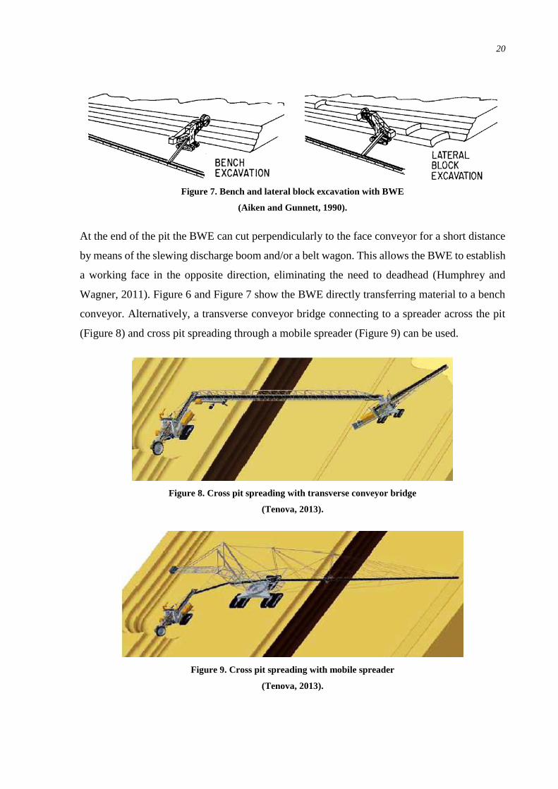
Figure 7. Bench and lateral block excavation with BWE
(Aiken and Gunnett, 1990).
At the end of the pit the BWE can cut perpendicularly to the face conveyor for a short distance
by means of the slewing discharge boom and/or a belt wagon. This allows the BWE to establish
a working face in the opposite direction, eliminating the need to deadhead (Humphrey and
Wagner, 2011). Figure 6 and Figure 7 show the BWE directly transferring material to a bench
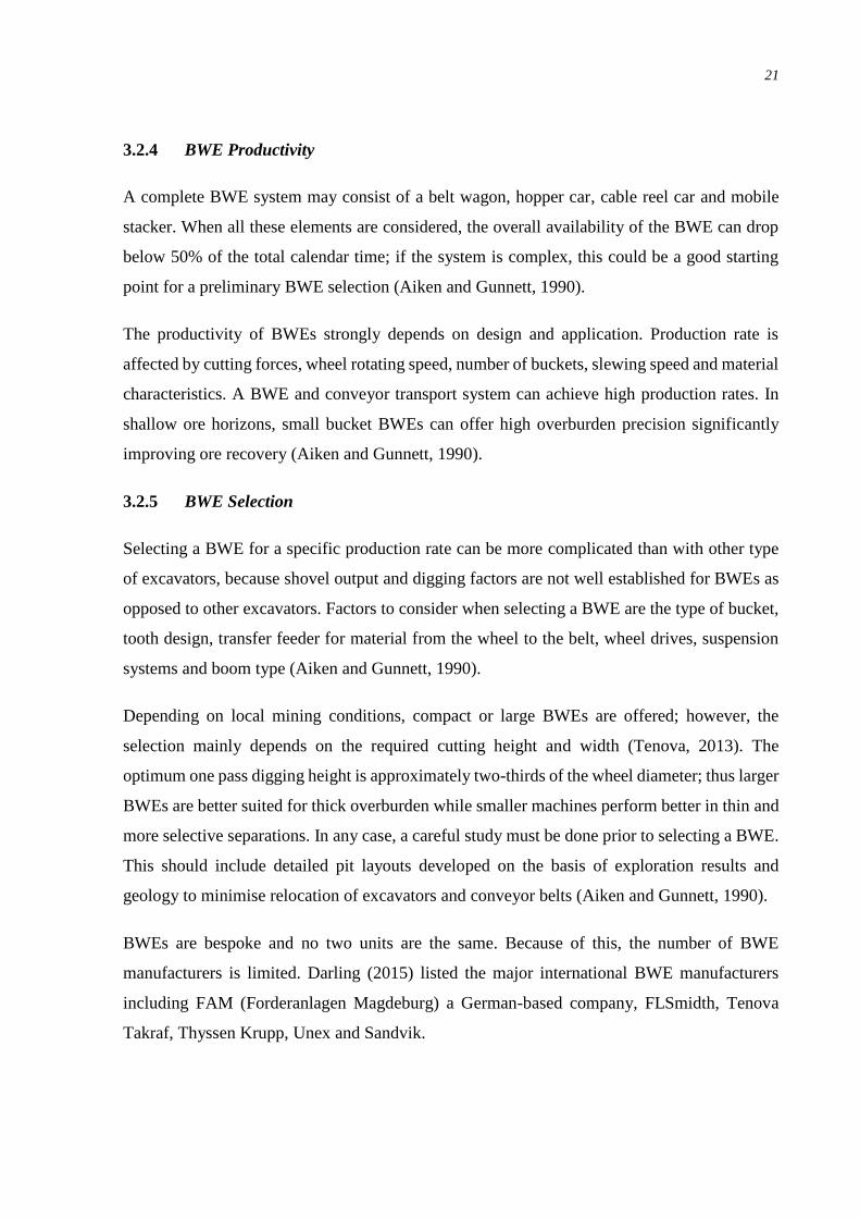
conveyor. Alternatively, a transverse conveyor bridge connecting to a spreader across the pit
(Figure 8) and cross pit spreading through a mobile spreader (Figure 9) can be used.
Figure 8. Cross pit spreading with transverse conveyor bridge
(Tenova, 2013).
Figure 9. Cross pit spreading with mobile spreader
(Tenova, 2013).
21
3.2.4 BWE Productivity
A complete BWE system may consist of a belt wagon, hopper car, cable reel car and mobile
stacker. When all these elements are considered, the overall availability of the BWE can drop
below 50% of the total calendar time; if the system is complex, this could be a good starting
point for a preliminary BWE selection (Aiken and Gunnett, 1990).
The productivity of BWEs strongly depends on design and application. Production rate is
affected by cutting forces, wheel rotating speed, number of buckets, slewing speed and material
characteristics. A BWE and conveyor transport system can achieve high production rates. In
shallow ore horizons, small bucket BWEs can offer high overburden precision significantly
improving ore recovery (Aiken and Gunnett, 1990).
3.2.5 BWE Selection
Selecting a BWE for a specific production rate can be more complicated than with other type
of excavators, because shovel output and digging factors are not well established for BWEs as
opposed to other excavators. Factors to consider when selecting a BWE are the type of bucket,
tooth design, transfer feeder for material from the wheel to the belt, wheel drives, suspension
systems and boom type (Aiken and Gunnett, 1990).
Depending on local mining conditions, compact or large BWEs are offered; however, the
selection mainly depends on the required cutting height and width (Tenova, 2013). The
optimum one pass digging height is approximately two-thirds of the wheel diameter; thus larger
BWEs are better suited for thick overburden while smaller machines perform better in thin and
more selective separations. In any case, a careful study must be done prior to selecting a BWE.
This should include detailed pit layouts developed on the basis of exploration results and
geology to minimise relocation of excavators and conveyor belts (Aiken and Gunnett, 1990).
BWEs are bespoke and no two units are the same. Because of this, the number of BWE
manufacturers is limited. Darling (2015) listed the major international BWE manufacturers
including FAM (Forderanlagen Magdeburg) a German-based company, FLSmidth, Tenova
Takraf, Thyssen Krupp, Unex and Sandvik.

22
3.2.6 IPCC
In-pit crushing and conveying (IPCC) is an alternative to the traditional truck and excavator
option (Utley, 2011). IPCC use fully mobile, semi-mobile or fixed in-pit crushers together with
conveyors and spreaders (for waste) or stackers (for ore) to extract material from a surface mine
(Sandvik, 2008). A spreader working on a waste dump and a semi-mobile in-pit crusher can be
seen in Figure 10 and Figure 11 respectively.
Figure 10. Waste spreader
(Turnbull and Cooper, 2009).
Figure 11. Semi-mobile crusher at the Mae Moh mine
(Turnbull and Cooper, 2009).
IPCC have significantly contributed to improving profitability through a reduction in
production costs. This has resulted from limiting the truck haulage to small distances of material
transport between the face and the crusher (Utley, 2011), or in some cases by totally replacing
trucks (Sandvik, 2008). These economies have allowed mines to operate economically with
lower ore grades, deeper pits and at higher capacities (Utley, 2011).

23
3.2.7 Types of IPCC
The three main types of IPCC systems are as follows:
Fully mobile. In this arrangement the shovel directly feeds the crusher, eliminating the
need for trucks almost completely. The crusher is mounted on tracks and moves with
the shovel (refer Figure 12). To connect the crusher to the main conveyor it is necessary
to use mobile connecting conveyors; namely belt wagons or grasshopper conveyors
(Turnbull and Cooper, 2009). Fully-mobile units are self-propelling. This is achieved
with crawlers, wheels, hydraulic pads or pneumatic pads, allowing them to relocate
every 1 to 10 days. Fully mobile units normally operate in tandem with a power shovel
at the face and an in-pit conveying system (Darling, 2015a).
Figure 12. Example of fully mobile in-pit crushing
(Metso, 2015).
Semi-mobile. These systems are placed close to the working face to reduce the haul
distance (refer Figure 11); this reduces the truck fleets. The crusher needs to be relocated
regularly, in some cases bi-annually, to maintain the system close to the working face
(Turnbull and Cooper, 2009). The units are mounted on steel legs, allowing relocation
using multi-wheel loaders or transport crawler beds. Semi-mobile plants are placed near
the centroid of the working area of the mine to reduce in-pit truck movement. They
relocate every 3 to 5 years. Some semi-mobile units however, are self-supporting and
rest on the pit floor. They relocate every 1 to 10 years (Darling, 2015a).
Fixed. These systems are located away from the mining face, at the pit boundary or at a
short distance out of the pit. These units stay at the same location for several years at a

24
time (Turnbull and Cooper, 2009); they relocate every 15 or more years (Darling,
2015a). In this case, the savings in trucking will be smaller because of the increased
distance from the mining face to the crusher (Turnbull and Cooper, 2009).
The above classification suggests that fully mobile systems may provide greater financial
benefits than semi-mobile or fixed options because the need for trucks is virtually eliminated.
However, Turnbull and Cooper (2009) comment that fully mobile systems are more complex
to implement, and that semi-mobile systems can be retro-fitted into existing open pit operations
without significantly altering the design or the schedule of the pit. Darling (2015) categorises
each method as shown in Table 4.
Table 4.
Comparison between IPCC options
IPCC Crushing Option Fully-mobile Semi-mobile Fixed
Throughput (t/h) < 10 000 < 12 000 < 12 000 Truck Quantity None Low Intermediate Crusher Type Sizers, jaw/double roll
crusher Any Any
Unit Crushing Costs Higher Intermediate Lower IPCC Conveying Options Dedicated ramp Conveyor tunnel Conveyor on haul road Conveyor Angle (°) < 18 < 10 < 6 Capital Costs Intermediate Highest Lowest Flexibility Intermediate Lowest Highest
Source: Darling (2015a)
3.2.8 IPCC Implementation
Regardless of the type of IPCC system, implementation must consider the location of the
crushing and conveying units as well as access for the loading equipment. The main difference
between a pit designed for IPCC and one designed for truck and shovel lies in the pushback
geometry. In IPCC, the optimum pushback is achieved with straightened pit walls. This will
maximise the conveyor span and minimise the number of transfer points. Wider pushbacks are
needed to accommodate the crusher station and temporary ramps. This can also reduce the
vertical advance rate, which will minimise crusher relocation (Turnbull and Cooper, 2009).
An optimised IPCC pit design will incorporate conveyor corridors and crusher stations in the
high walls, and it will take advantage of natural changes in the geometry to place crusher
stations and transfer points. How the conveyor will exit the pit is also important; this can
normally be done in three ways (Turnbull and Cooper, 2009).

25
1. Tunnels: Applicable if the topography restricts the use of trucks or other alternatives.
2. Dedicated conveyor ramps: These type of ramps are better suited to fixed crushers because
for semi-mobile systems it is difficult to design and implement. Dedicated ramps can be
much steeper than haul roads; however, access is still required for maintenance.
3. Existing haul road: When both trucks and IPCC system are in place, the IPCC conveyor
and a haul road will cross over. Therefore, a conveyor bridge or a conveyor tunnel will be
necessary. In a conveyor bridge, the conveyor is elevated such that there is enough clearance
for a fully loaded truck to travel below. In a conveyor tunnel, a short tunnel is constructed
under the haul road. When an IPCC conveyor is retro-fitted to an existing haul road, the
road width needs to be extended between 7 and 9 m to add a conveyor corridor. An example
of a conveyor corridor and haul road can be seen in Figure 13.
Figure 13. IPCC haul road example
(Turnbull and Cooper, 2009).
In semi-mobile and fixed systems, the location of the crusher and access for the loading
equipment are also important. Turnbull and Cooper (2009) propose three layouts:
1. The semi-mobile crushing station is located in the highwall at a designed location along the
haul road. Trucks access the crusher off the haul roads, as illustrated in Figure 14.
2. The crusher is located at a temporary location inside the haul road and trucks access the
crusher from the bench through a temporary ramp. Once the crusher has been relocated, the
crusher pad and the temporary ramp are removed. This is displayed in Figure 15. This
demands increased planning efforts and costs related to construction and removal of the
crusher and pad ramp.
Steel pin to constrain concrete bund
37% truck 2.9 m
75% truck 5.7 m
37% truck 2.9 m 7.7 m 7.7 m
1.0 m
2.0 m
2.4 m 2.0 m
39.3 m
8 m conveyor allocation
25.9 m 3.5x truck

26
3. The crusher is temporarily located on the pit side of the haul road and trucks gain access
through a conveyor bridge off the haul road. Once the crusher is relocated, a temporary
ramp is built to facilitate the removal of the crusher pad as shown in Figure 16. Removal of
the crusher pad is a slow and expensive process normally limited to two benches.
Figure 14. Semi-mobile crusher station designed in the wall
(Turnbull and Cooper, 2009).
Figure 15. Semi-mobile crusher station accessed through a temporary ramp
(Turnbull and Cooper, 2009).

27
Figure 16. Semi-mobile crusher station accessed from the haul road
(Turnbull and Cooper, 2009).
3.2.9 IPCC Productivity
The key piece of equipment that drives productivity in an IPCC system is the crusher. Utley
(2011) adds that three fundamental criteria should be assessed when selecting the crushing unit.
1. Type and characteristics of the ore. This will determine the type of crusher needed.
2. Plant capacity. This will determine the size of the crusher.
3. Plant layout and design.
Different types of crushers exist in the market, including gyratory, jaw and roll crushers, and
the IPCC system can be supplied with almost any type of primary rock crushing unit. However,
the most commonly selected types are low-speed sizers and double-roll crushers (Utley, 2011).
Primary crushers are used in the first stage of the size reduction cycle. For large capacities, the
type of crusher normally used includes the gyratory and double roll crushers, as well as the low
speed and hybrid roll sizers (Utley, 2011). Darling (2015a) adds that whilst almost any type of
primary crusher can be used, gyratory crushers are the most commonly used in a mobile plant,
which can operate with a sustained level of up to 9000 t/h. Jaw crushers are better suited for
low tonnage operations and double roll crushers are better fitted for relatively soft and non-
abrasive feeds.

28
3.2.10 IPCC Selection
Mine planners commonly select fully mobile continuous mining systems for soft-rock
applications (Utley, 2011). However, IPCC systems are not off-the shelf items. Technical and
economic factors that should be considered when selecting IPCC systems are the layouts of the
equipment in the pit, productivity, interaction with the drill, blast and bench operation sequence,
ease of relocation, flexibility in changes in the reserve, scalability and compatibility with other
components in the system (Atchison and Morrison, 2011).
Atchison and Morrison (2011) add that an IPCC system must satisfy two competing criteria:
1. Be physically able to excavate and deliver material to an out-of-pit system at a required
capacity; and
2. Be cost-effective to an acceptable level during the capital and operating phases of the
operation.
When assessing these criteria, Atchison and Morrison (2011) have assumed that the mine layout
and the type of material are amenable to strip mining and favoured by IPCC systems, a system
exists downstream to receive the material from the conveyor, and a reliable power supply exists
which is cost-effective. These authors note that if these assumptions cannot be confidently
confirmed, then the suitability of an IPCC system is questionable.
Darling (2015a) mentions some of the currently relevant IPCC system providers including,
BMT-WBM, FLSmidth, Joy Global, Sandvik, Tenova Takraf, Metso and Thyssen-Krupp.
3.2.11 Advantages and disadvantages of IPCC systems
Utley (2011) assessed the advantages and disadvantages of IPCC systems against those of truck
and shovel. The advantages of conveyor haulage compared to truck haulage include the
following.
Reduced costs. The distance between loaders and crusher is reduced.
Reduced operating costs from consumables (tyres, fuel and lubricants).
Reduced maintenance costs of haul roads.
Reduced labour costs resulting from shorter haulage distance and less trucks; thus less
operators and maintenance personnel.

29
Reduced safety risks.
IPCC offers greater predictability of future costs in long-term mining operations.
Conveyors can traverse grades of up to 30% compared to the 10% to 12% that trucks
can do (Seib, 2016).
Conveyors can easily cross roads, railways, waterways, and other obstructions.
Conveyors are more energy efficient than trucks, emit lower CO2 and require less skilled
maintenance labour.
IPCC allows maximum operational availability.
The system is less susceptible to weather conditions (fog, rain, snow and frost).
Continuous flow of material can be achieved with conveyors.
In-pit crushing stations have equal performance and integrity as traditional crusher
stations. This allows flexibility in long term planning.
Utley (2011) identified the following disadvantages of IPCC systems.
Reduced short-term flexibility as opposed to trucks.
High relocation costs of overland conveyors and high upfront costs.
Deficient truck capacity to feed the process while the semi-mobile crusher is relocated.
Conveyor systems are more sensitive to shortage of parts, especially in remote areas.
IPCC systems are less capable of achieving increased capacities than trucks.
Conveyors are less flexible in ore blending processes.
Conveyors require the material to be crushed prior to transport.
Reliability of the individual components of IPCC systems is critical since downtime of
any single component will shut down the whole system.
IPCC systems require continuous monitoring.
Productivity of the IPCC highly depends on the loading system, but keeping a constant
maximum production is not guaranteed.
3.3 APPLICATION OF BWE AND IPCC SYSTEMS TO SURFACE MINING
At present, most open pits in Australia are mined with traditional truck and shovel mining
systems, which are flexible to adapt to pit geometry, production rate and poor mine planning
practices. Mine owners have the option of owning and operating the mining fleet or engaging
contractors to supply and manage the fleet (Turnbull and Cooper, 2009).

30
3.3.1 Continuous Mining Systems
Continuous mining systems primarily depend on the type and properties of the ore being mined.
For instance, in the case of loose and light earth, BWE technology in combination with a
conveyor system can offer the advantages of continuous mining. However, to mine harder ore,
it is necessary to use crushers to reduce the ROM ore to a conveyable size. A characteristic of
continuous open pit mining technology is its long expected life (Utley, 2011).
The objective of fully mobile continuous crushing systems is to eliminate the need for trucks.
This is achieved by having the shovel feed the ROM ore directly into a continuous materials-
handling system. In this case, the crusher needs to be fully mobile and be able to follow the
movement of the shovel. It must be designed to follow the movement of the shovel boom and
bucket, and match the operating capacity of the shovel. Usually, an existing cable or hydraulic
shovel can be used if a mobile crushing plant replaces the truck fleet (Utley, 2011).
Darling (2015a) indicates that IPCC is most attractive when the mine life exceeds ten years,
when hauling uphill is required or the trucking distances are too long, a large and steady tonnage
of material is to be moved, minimising carbon and dust emissions is important and there are no
more than three types of materials to work with.
3.4 TECHNICAL REQUIREMENTS TO IMPLEMENT BWE AND IPCC SYSTEMS
BWEs are typically used for unconsolidated materials with relatively limited capacity for rocky
materials. They also need linear, flat-floored mining faces that advance in straight or radial
patterns to accommodate their conveyors. BWEs can operate in linear pits with a parallel
spoiling process to fill a void at a short distance or in multiple benches in deep pit mines with
outside spoil dumps. The BWE is a high capital yet low operating cost system with limited
flexibility. It can operate in a limited range of applications and is susceptible to geologic
variance. These machines are highly customised, robust in design and with long lives
(Humphrey and Wagner, 2011).
Operating and capital costs can be reduced with good mine layouts with BWE (Aiken and
Gunnett, 1990) and IPCC (Cooney, 2016c). Large BWEs are only suitable for long-term
operations due to their high capital cost (Aiken and Gunnett, 1990). This is also true for IPCC

31
(Darling, 2015a). BWEs and IPCC can compare well against draglines and power shovels in
the following aspects (Aiken and Gunnett, 1990 and Cooney, 2016c):
Instantaneous power demand;
Weight to output ratio;
Loading shocks; and
Power consumption.
BWEs can also provide these benefits (Aiken and Gunnett, 1990):
They operate in wider benches and more stable pit slopes exposing more reserves;
They improve shovel’s efficiency in soft rock when the BWE removes soft overburden;
They have better control for selective mining;
They can deliver material above and below the working level; and
They can perform high and/or deep cuts.
IPCC can provide similar benefits to those mentioned above. In early stages of a project, key
questions that need to be answered in particular to select IPCC are (Blunck, 2016):
What is the life of mine and annual production;
What is the available operating time to achieve production and manpower;
What is the geology of the deposit; and
How does the price of electricity compare to that of diesel.
Higher level questions for IPCC selection include (Blunck, 2016):
What is the rock strength;
What is the size and shape of cut/push backs;
What dump area is available;
How many ore grades are involved; and
Are downhill hauls required?
32
GEOTECHNICAL CONDITIONS ASSESSMENT
Insite Geology was engaged by NHG to conduct a field investigation into the geotechnical
conditions within the mining lease. A core drilling programme was completed in 2008 which
comprised seven drill holes, with one of the drill holes abandoned and replaced with an
alternative. The study was carried out through geotechnical HQ and core drilling. The results
from the 2008 study were presented in a report compiled in 2009 (Insite Geology, 2010).
A second geotechnical drilling and laboratory testing study was completed between late 2009
and early 2010, to further assess the conditions for the initial box-cut for the mining operation.
This study included six vertical drill holes distributed throughout the lease, following the same
procedure used in 2008 (Insite Geology, 2010).
In both cases the study consisted of lithological and geotechnical logging of core including
density, gamma and caliper downhole geophysical logs (Insite Geology, 2009 and Insite
Geology, 2010). The standing water levels (swl) were also measured during the 2008 study.
Laboratory testing focused on samples of weathered and fresh overburden as well as fresh coal
and interburden (Insite Geology, 2009).
4.1 GEOLOGICAL SETTING
The middle Jurassic age Juandah Coal measures are the target coal-bearing unit for the Wombat
Project. The Juandah and the Taroom Coal measures form a stratigraphic section that is
comparable to the Walloom Coal measures further east. The Juandah Coal measures comprise
five main seam groups: UG, Y, A, B and C seams, which increase in depth below the natural
surface. These seams and plys are schematically represented in Appendix 3 while Figure 17
shows a stratigraphical cross-section at the Wombat lease where these seams can be
appreciated. As seen in Figure 17, the coal seams are separated by interburden units consisting
of variably interbedded to massive sandstone, siltstone and carbonaceous mudstone (Insite
Geology, 2009).
Two main faults have been identified at the lease, both trending north-west. Fault A has inferred
throws of up to 8 m and Fault B of up to 35 m. This resulted in a graben-style downthrown
block between these two faults. Faulting affects the sub-crops of the upper seams but the limits

33
on the main seams are not affected. Stratigraphic bedding within the Juandah Coal measures is
sub-horizontal to gently dipping at less than 3° (Insite Geology, 2009).
Figure 17. Stratigraphical cross-section at the Wombat Project
(NHG, 2013).
4.2 GROUNDWATER
The standing water levels were determined from 102 geotechnical drill holes collected across
the lease. These results are summarised in Table 5, and focus mainly on the relative location to
Horse Creek (Insite Geology, 2009).
Table 5.
Summary of standing water levels at the Wombat lease
Area/location Standing water levels below ground surface (m)
Minimum Maximum Average Elevated area north-west of Horse Creek 14.14 32.88 20.94 Elevated area west of road and Horse Creek 12.13 24.36 17.00 Horse Creek floodplain 2.67 10.80 7.99 Elevated area east of road and Horse Creek 17.59 38.30 24.14
Source: Insite Geology (2009)
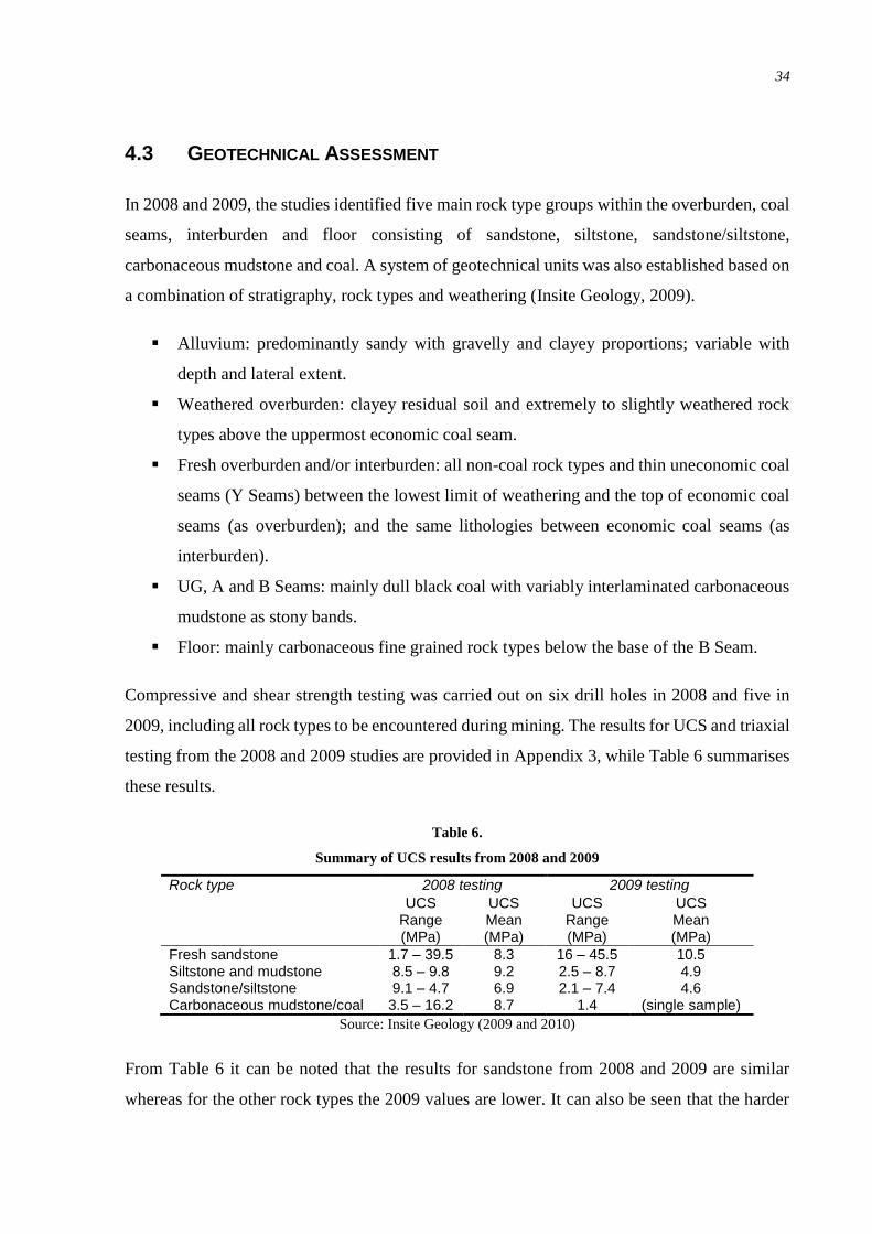
34
4.3 GEOTECHNICAL ASSESSMENT
In 2008 and 2009, the studies identified five main rock type groups within the overburden, coal
seams, interburden and floor consisting of sandstone, siltstone, sandstone/siltstone,
carbonaceous mudstone and coal. A system of geotechnical units was also established based on
a combination of stratigraphy, rock types and weathering (Insite Geology, 2009).
Alluvium: predominantly sandy with gravelly and clayey proportions; variable with
depth and lateral extent.
Weathered overburden: clayey residual soil and extremely to slightly weathered rock
types above the uppermost economic coal seam.
Fresh overburden and/or interburden: all non-coal rock types and thin uneconomic coal
seams (Y Seams) between the lowest limit of weathering and the top of economic coal
seams (as overburden); and the same lithologies between economic coal seams (as
interburden).
UG, A and B Seams: mainly dull black coal with variably interlaminated carbonaceous
mudstone as stony bands.
Floor: mainly carbonaceous fine grained rock types below the base of the B Seam.
Compressive and shear strength testing was carried out on six drill holes in 2008 and five in
2009, including all rock types to be encountered during mining. The results for UCS and triaxial
testing from the 2008 and 2009 studies are provided in Appendix 3, while Table 6 summarises
these results.
Table 6.
Summary of UCS results from 2008 and 2009
Rock type 2008 testing 2009 testing
UCS Range (MPa)
UCS Mean (MPa)
UCS Range (MPa)
UCS Mean (MPa)
Fresh sandstone 1.7 – 39.5 8.3 16 – 45.5 10.5 Siltstone and mudstone 8.5 – 9.8 9.2 2.5 – 8.7 4.9 Sandstone/siltstone 9.1 – 4.7 6.9 2.1 – 7.4 4.6 Carbonaceous mudstone/coal 3.5 – 16.2 8.7 1.4 (single sample)
Source: Insite Geology (2009 and 2010)
From Table 6 it can be noted that the results for sandstone from 2008 and 2009 are similar
whereas for the other rock types the 2009 values are lower. It can also be seen that the harder

35
rock type is sandstone and the maximum UCS value that can be expected is in the order of
46 MPa. The shear strength of the discontinuities for laminated rock types was tested in 2008
while in 2009, both laminated and non-laminated rock types were analysed. These results are
found in Appendix 3 where it can be seen that the peak cohesion was in excess of 134 kPa in
laminated rock types.
In regards to the material excavatability, Insite Geology (2009) established that the box cut and
initial ramp excavation would be made through weathered overburden at the line of oxidation.
Excavation would then continue through fresh overburden along the top of coal to form the
initial endwalls and highwalls of the pit. The free-dig depth would range between 10 to 12 m
within weathered overburden, depending on the size of the excavation equipment. Blasting
would be required for fresh overburden and interburden rock types as well as the coal seams to
ensure efficient excavation.
Following the review of the geotechnical data and since it is expected that the overburden will
require blasting, it was found that the BWE would not be attractive as a continuous mining
option. The main reason being that free-digging the overburden with a BWE is not guaranteed.
Thus, from this point forward, the project focused on implementing an IPCC system.
4.4 STRIPPING HORIZONS AT THE WOMBAT PROJECT
In the present study, several cross-sections and rainbow plots were created in Minescape using
the existing geological model. Appendix 3 provides two of these cross-sections as an example.
The purpose was to understand the physical distribution of the different lithologies and to
identify the limiting stripping horizons that would be suitable for the proposed IPCC system.
This was also done to identify the areas of the lease where mining can start; mainly based on
areas of thicker coal and thinnest overburden since this will allow accessing the coal in the
shortest time, providing early cash flows in the life of the operation.
In discussion with the Client, it was agreed that for both cases, the same block model as created
for the dragline assessment would be used to allow a direct comparison, mining along strike
(Cooney, 2016a). In this case, blocks of 70 m x 100 m were used to develop the Minescape
plots and the same results were obtained as in the dragline case. This can be seen in Figure 18
to Figure 20, which agree with the results for the existing mine plan (Appendix 2).

36
Figure 18. Topography at the Wombat Project.
From Figure 18 it was concluded that the variation in surface terrain ranged between RL 240
and 290, thus a variance of around 50 m throughout the lease. Figure 19 shows that the thickest
overburden lies at the southern part of the lease, between 45 and 60 m thick. However, most of
the overburden within the lease boundaries ranges between 10 and 20 m thick. There is a region
towards the south-east of the lease where the overburden thickness varies from 30 to 40 m.

37
Figure 19. Overburden thickness at the Wombat Project.
Examining Figure 20 it was found that the thickest coal lies at the centre of the lease, ranging
between 12 and 14 m. The thick coal area extends towards the southern edge of the mining
lease; however thin coal layers are found towards the western bounds. There is a pocket of low
coal thickness in the northern area, averaging 1 to 2 m thick.

38
Figure 20. Coal thickness at the Wombat Project.
Since it was assumed that the IPCC could be modelled using the dragline scenarios, the same
stripping horizon was applied in this case. Thus, the pit floor was at the bottom of the C1 seam.
4.5 INFRASTRUCTURE REQUIREMENTS
4.5.1 IPCC Equipment Selection
The selection of the equipment depended on the mining horizons that were established. For the
IPCC system, the primary equipment was the shovel that would feed the crusher. A fully mobile
arrangement was preferred because there would be greater savings by eliminating the need of a
truck fleet for overburden removal. A bench height of 18 m was adopted because of suitability
for the largest rope and hydraulic shovels currently available. A Caterpillar 7495 Rope Shovel
and a Liebherr R9800 Hydraulic Face Shovel were considered.

39
For this concept study, the layout shown in Figure 21 was assumed. It was also assumed that
the working area for the IPCC system would be at least 180 m wide. In consultation with a
manufacturer, the equipment outlined in Table 7 was proposed for the layout. It was also
assumed that the equipment in Table 7 would demand 60% of its installed power (Rokovic,
2016). A total of 6 operators would be needed to handle the system (Blunck, 2016).
Table 7.
IPCC Equipment requirements
Equipment Installed Power (kW)
Fully Mobile Crusher 2000 Mobile Conveyor Bridge 700 Conveyor Belt System (9 km) 6000 Tripper Car 350 Spreader 850
Source: Rokovic (2016)
Figure 21. IPCC conceptual layout.
4.5.2 IPCC System Working Method
The proposed IPCC system would work as follows (Refer Figure 22). A shovel excavator (1)
will remove the material and will dump it into the feed hopper (2) of the mobile crusher. The
material will then be transported by an apron feeder (3) to the top of the crusher (4) which will
reduce the size of the material. The slewing discharge conveyor (5) will dump the material on
a mobile bridge (6) which will then transport the material onto the supporting chute and on the
conveying system (7). Power for the complete system would be supplied via a cable reel car.
The mobile crushing plant will be supported on an electric driven crawler track assembly. The
superstructure with feed hopper bin, apron feeder, double-roll crusher and slewing discharge
boom will be supported on the substructure. The discharge boom with turntable can slew on the
superstructure and be supported on a cantilever arm of the main frame superstructure (Rokovic,
2016). In Figure 22 the red arrows show the direction in which the material will travel.
CONVEYOR
SHOVEL
CRUSHER
SPREADER

40
Figure 22. Proposed IPCC system
(Rokovic, 2016).
Once the strip has been mined, all the infrastructure will be shifted to the next working strip
using the crawlers they will be mounted on. For conveyors, two main types would be used:
Shiftable conveyors (face and dump conveyors).
Relocatable conveyors.
Each conveyor module will be mounted on sleepers and the modules will be shifted with track
dozers or pipe layers and shifting attachment. Figure 23 displays a pipe layer arrangement.
Figure 23. Pipe layer arrangement
(Rokovic, 2016).
1
2
3
4
5
6
7

41
MODELS
5.1 XPAC MODELS
After creating the plots and cross-sections in Minescape, several ranges were developed in
XPAC based on the Minescape block model. A target production rate of 5 Mtpa was assumed
at a stripping ratio cut-off of 7:1, which is the same as one of the scenarios examined for the
dragline case. This yielded approximately 35 Mtpa of overburden removal that the equipment
must achieve. Different input paths were created in XPAC for each type of prime overburden
removing equipment; namely truck and excavator, and IPCC. To create these input paths, two
main pits were defined to schedule in XPAC, where pits A, B, C and D are the same as shown
in Appendix 2:
Pit 1: Included Pits C and D, and would be mined by IPCC.
Pit 2: Included Pits A and B, and would be mined by truck and excavator due to the
smaller size of these pits.
XPAC was run to update the input path for the equipment. For this purpose, a new XCM script
was written so that the software could identify between coal seams that were not continuous
throughout the lease. An XCM script is a coding tool in XPAC which can be written to tell the
software to carry out specific actions based on logic conditions.
5.1.1 Reserves Modelling
Since the reserves extracted from the geological model were based on a strip and block layout,
it was necessary to convert these raw in-situ reserves to mineable reserves to schedule them in
XPAC. This was done using the same assumptions from the previous XPAC models (Table 2,
Section 2.2) and using an XCM script to incorporate them into the new model.
After running XPAC, several scheduling plots were generated assuming 18 m high benches for
the IPCC, using the largest rope shovel or hydraulic shovel currently available. The maximum
bench height for the IPCC was defined at 30 m (Cooney, 2016b). These plots are provided in
Appendix 4, and they showed that the B seam was a possible pit floor. However, it was decided
to also investigate the viability of mining the C seam, but the analysis showed that it was not

42
worthwhile to pursue this seam because of potential physical constraints for the conveying
infrastructure. Therefore, the pit floor for IPCC was defined at the B seam.
Examining the overburden and interburden between the Y to C seams it was noted that the
interburden for the C1 seam was a good candidate for IPCC and so was the interburden for B1
towards the south. However, the interburden for the Y1 and A1 seams were deemed too thin.
After establishing the suitable mineable reserves for IPCC, the scheduling plots in Appendix 4
were used to generate a new XPAC model after creating the following new activities:
0: Dump.
1: Overburden.
2: Parting loader.
3: Parting excavator.
4: Coal.
A new XCM script was written to enable XPAC to allocate a path for the overburden and
interburden, based on each activity. To do this, these assumptions were made (Cooney, 2016c):
If the thickness was between 0 and 18 m, IPCC was used. A large electric rope shovel
was selected as the IPCC excavator to maximise throughput; however, this excavator
offers reduced selectivity when cutting into the interburden.
If the thickness was between 18 m and 30 m, IPCC pre-stripping with dozer push was
used where the dozer would push the material down to the shovel, to suit the shovel’s
maximum working range.
If the thickness was between 30 and 40 m, post-stripping with an excavator was used.
This excavator would remove what the IPCC excavator didn’t. To improve material
selectivity and minimise dilution, a smaller hydraulic excavator was considered to
remove the overburden above the coal after the IPCC had passed.
Based on these assumptions, it was possible to generate an XPAC plot showing the positive
cash flow for overburden stripping, as shown in Figure 24. After this assessment, an input path
was created for the IPCC case using the same Pit 1 and Pit 2 assumptions explained above. It
must be emphasised that this positive cashflow plot was produced based on the inputs of the
2013 model, which used a long-term average Newcastle standard coal price that was energy
adjusted for the Wombat deposit.

43
Figure 24. Maximum cash flow positive XPAC plot for IPCC.
After creating the input paths and assigning the equipment to each activity, the new schedule
was ready to be run. In XPAC it is possible to schedule according to the following conditions:
Target production schedule: aims at achieving a set production target.
Production rate schedule: based on the physical capacity of the equipment on an hourly
basis.
Destination schedule: considers sending the equipment to different locations within the
mine, for instance to different dumps.

44
Again, a 5 Mtpa production rate target schedule was run resulting in 150 Mt reserves. Pit 1 had
a life of 30 years while Pit 2 finished earlier with a life of 8 years. It was required that Pit 2
finished earlier to allow for tailings storage capacity in the mined-out void. There was a variance
of about 4.27 Mtpa in the last year with respect to the 5 Mtpa target. This variance was divided
into ¾ rounded up and ¼ rounded down. An XCM script was created in XPAC to assign this
variance in production. Consequently, the mining rate for Pit 1 also had to be adjusted to ensure
the target rate of 5 Mtpa of product coal was met. The schedule was re-run in XPAC and an
output was produced, mainly providing the volumes of overburden and coal assigned to each
equipment in each pit. This XPAC model output was used to develop a production schedule.
5.2 EXCEL MODELS
After reviewing the literature and past work on this project, the next step in the methodology
was to build a mine schedule using the XPAC output. Initially three models were built:
An IPCC model considering a large rope shovel (CAT7495);
An IPCC model considering a smaller hydraulic face shovel (R9800); and
A truck and excavator case as a baseline for comparison (TEX).
At the initial stages of the project, it was expected that a large rope shovel would produce the
best results due to its higher capacity, improving its utilisation. However, after discussions with
equipment manufacturers, it was advised to consider a smaller face shovel due to its lower
capital cost which would improve the project’s net present value (NPV). The results from each
of the above cases would then be compared to the 2015 dragline case.
5.2.1 Production Schedule
For each scenario, the XPAC output was exported to Excel. This detailed the annual volume of
waste (overburden and partings) and tonnage of coal to be moved in each pit for the LOM. This
included prime and rehandled volumes for different types of equipment. For this purpose, the
primary equipment shown in Table 8 was adopted for material movement. The XPAC model
also provided the ROM tonnes and volume of coal as well as the product tonnes.

45
Table 8.
Primary equipment allocated to each material and pit
Equipment Type Purpose Pit 1 Pit 2
Caterpillar 7495HR
Electric Rope Shovel
Prime IPCC Excavator Yes – strip overburden and feed crusher
No
Liebherr R9800
Hydraulic Face Shovel
Prime IPCC Excavator Yes – strip overburden and feed crusher
No
Caterpillar 6060BH
600 t Hydraulic Excavator
Remove overburden and partings
Yes – post-strip overburden and
partings > 1 m thick
Yes – prime
overburden Hitachi EX3600
400 t Hydraulic Excavator
Strip overburden and balance annual hours
Yes Yes
P&H L1150 Front end loader Remove partings < 1.5 m thick and coal mining
Yes Yes
Figure 25 shows the XPAC waste volumes for both pits where the volumes were allocated to
the equipment in Table 8 using an IPCC model. Figure 25 shows that the overburden (OB) was
assigned to the IPCC but in the excavator model, this volume was allocated to the 600 t
excavator.
Figure 25. Raw waste volumes from XPAC for both Pits.
From Figure 25 it is clear that the IPCC was moving a low volume of waste in the first year of
operation. To improve the utilisation of the IPCC system, its implementation was delayed to
start in year 2 of production and the waste from year 1 was allocated to the 600 t excavator.
This also delayed the capital expenditure of the IPCC by one year.
In each pit, the material was balanced between the 600 t and 400 t excavators by bringing
volume forward to improve the utilisation of the equipment. The purpose was to balance the
annual operating hours of each piece of equipment. To achieve this, the volumes allocated to
0
10
20
30
40
50
60
70
80
1 2 3 4 5 6 7 8 9 10 11 12 13 14 15 16 17 18 19 20 21 22 23 24 25 26 27 28 29 30
Waste
Vo
lum
e (
Mb
cm
)
Year
IPCC OB IPCC Exc. OB Poststrip Excavator OB Parting FEL Excavator Parting

46
the 600 t excavator were prioritised and excess volumes were assigned either to additional 600 t
excavators, a smaller 400 t excavator or a combination of both such that each piece of
equipment was close to its maximum annual production rate. After balancing the waste
movement, the waste mining schedules were produced for each model, as shown in Appendix
5, where it can be seen that the utilisation of the IPCC system was optimised.
The production data from each pit was then combined into volumetric and product quality
results. It must be noted that for this project it was assumed that only “Gold” quality product
will be sold following current NHG’s coal market specifications. This product quality was
assessed in terms of energy on a Gross As Received (GAR) basis and compared to the
Newcastle Index thermal coal price, which uses a specific energy reference of 6322 kcal/kg.
The GAR calculation includes the latent heat of the moisture within the coal, which lowers the
effective calorific value of the product in the boiler (Knowledge Infrastructure Systems, 2016).
This also reduces the sell price of the coal, affecting the revenues. The average GAR of the
Wombat deposit is 5823 kcal/kg (NHG, 2013) or 92.1% of the Newcastle standard benchmark.
5.2.2 Primary Equipment Productivity
The production schedules were used to plan the equipment volume allocation. This was done
based on volume of material per period, equipment annual hours and productivity. The
equipment annual hours were based on a Time Usage Model (TUM) for the primary loading
equipment. The TUM establishes the number of hours that are lost due to the effects of weather,
planned and unplanned maintenance, operational delays, imposed non-working time (public
holidays), and non-operational non-working time (crew travel time). However, the TUM
excludes major shutdowns because these are not annual events. Appendix 6 provides an
example of a typical TUM structure.
The TUM model is developed for the prime overburden-handling unit, as this is the main dirt
moving equipment. Therefore, a different TUM was used for the excavators and dragline. The
TUM for an IPCC system has some variation to the previous cases because the different
equipment involved in material movement must be considered. In other words, each IPCC
component has its own TUM, which make-up the TUM for the IPCC system. This includes the
shovel, crusher, conveyors and spreader. Equipment availability and utilisation were also taken
into account when developing the TUM.

47
In this concept study, availability was determined from experience, based on the percentage of
time the equipment is expected to spend in maintenance. Normally, experienced maintenance
personnel are involved in establishing the percentage of time needed for each level of
maintenance and for each piece of equipment, making an allowance for the expected useful life
of individual components and the time to service or replace such components. Once the actual
operating time for a year is determined, it is possible to estimate equipment utilisation. In the
case of an IPCC system, availability and utilisation are a function of each of the main
components (Blunck, 2016). After establishing a TUM for the IPCC system and based on an
existing NHG TUM for truck and shovel, the annual operating hours for each excavating unit
were determined as shown in Table 9.
The productivity for each of the primary equipment was assumed as shown in Table 9. The
productivity for the IPCC’s rope shovel was based on previous benchmarking data (Cooney,
2016d), while the values for the IPCC’s face shovel were advised by an equipment
manufacturer (Blunck, 2016a). It must be noted that both shovels for IPCC are electrically
driven machines. For other equipment, the productivities were NHG internal benchmark values
(Cooney, 2016d). The equipment operating hours and productivity assumptions resulted in the
annual production also shown in Table 9.
Table 9.
Productivity assumptions for primary equipment
Equipment Annual Hours (h)
Productivity (bcm/h)
Annual Production (kbcm/y)
IPCC CAT7495 (Rope Shovel) 5800 3000 17 400 IPCC R9800 (Face Shovel) 5200 2400 12 480
RH340 (600 t excavator) 6100 2250 13 725 EX3600 (400 t excavator) 6000 1400 8540
P&H L1150 (FEL) 6000 1000 6000
Source: Blunck (2016a) and Cooney (2016d)
5.2.3 Ancillary Equipment
Several ancillary machines were selected as detailed in Table 10. Some of the equipment was
selected based on hourly production rates while for others, annual operating hours were used.
The pit dozer’s hours were estimated as 60% of the shovel or excavator hours (Cooney, 2016d).
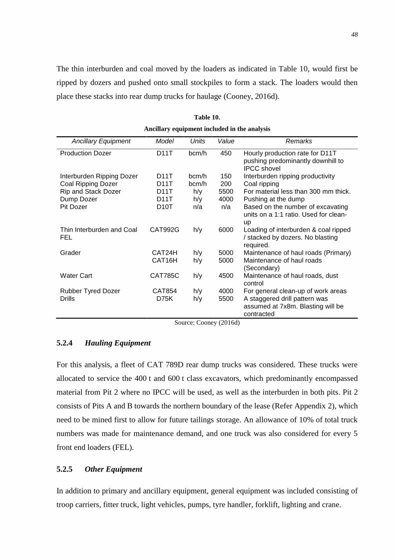
48
The thin interburden and coal moved by the loaders as indicated in Table 10, would first be
ripped by dozers and pushed onto small stockpiles to form a stack. The loaders would then
place these stacks into rear dump trucks for haulage (Cooney, 2016d).
Table 10.
Ancillary equipment included in the analysis
Ancillary Equipment Model Units Value Remarks
Production Dozer D11T bcm/h 450 Hourly production rate for D11T pushing predominantly downhill to IPCC shovel
Interburden Ripping Dozer D11T bcm/h 150 Interburden ripping productivity Coal Ripping Dozer D11T bcm/h 200 Coal ripping Rip and Stack Dozer D11T h/y 5500 For material less than 300 mm thick. Dump Dozer D11T h/y 4000 Pushing at the dump Pit Dozer D10T n/a n/a Based on the number of excavating
units on a 1:1 ratio. Used for clean-up
Thin Interburden and Coal FEL
CAT992G h/y 6000 Loading of interburden & coal ripped / stacked by dozers. No blasting required.
Grader CAT24H CAT16H
h/y h/y
5000 5000
Maintenance of haul roads (Primary) Maintenance of haul roads (Secondary)
Water Cart CAT785C h/y 4500 Maintenance of haul roads, dust control
Rubber Tyred Dozer CAT854 h/y 4000 For general clean-up of work areas Drills D75K h/y 5500 A staggered drill pattern was
assumed at 7x8m. Blasting will be contracted
Source: Cooney (2016d)
5.2.4 Hauling Equipment
For this analysis, a fleet of CAT 789D rear dump trucks was considered. These trucks were
allocated to service the 400 t and 600 t class excavators, which predominantly encompassed
material from Pit 2 where no IPCC will be used, as well as the interburden in both pits. Pit 2
consists of Pits A and B towards the northern boundary of the lease (Refer Appendix 2), which
need to be mined first to allow for future tailings storage. An allowance of 10% of total truck
numbers was made for maintenance demand, and one truck was also considered for every 5
front end loaders (FEL).
5.2.5 Other Equipment
In addition to primary and ancillary equipment, general equipment was included consisting of
troop carriers, fitter truck, light vehicles, pumps, tyre handler, forklift, lighting and crane.

49
5.2.6 Capital and Replacement Schedule
Once the production schedule was completed considering the primary, ancillary, hauling and
other equipment, a capital and replacement schedule was developed. Capital expenditure was
divided into infrastructure and equipment. Infrastructure capital for an IPCC system using a
face shovel is outlined in Table 11, which also shows the asset life assumed for depreciation. A
straight line depreciation regime was adopted for this project.
Table 11.
IPCC face shovel infrastructure capital and depreciable life assumptions
Infrastructure Capital Expenditure Capital Expenditure
(AUDm) Depreciable Life (Years)
Capitalised Development 25 20 Land Purchase 22.5 20 Coal Handling and Processing Plant (CHPP) 180 20 Horse Creek Diversion 6 18 Accommodation Village 40 20 External and Internal Public roads 28 20 Mine Industrial Area 25 20 Water Management 25 20 On site Power and Communications 66 20 Tailings Dams 57 10 Rail - Link and loop to Surat Basin Rail Line 143 20 Design and Project Management 31 20 Contingency 78 20 IPCC (excluding shovel) 135 30
Source: NHG (2013) and Rokovic (2016)
It should be noted that in Table 11 the infrastructure capital for rail only considered the cost for
transporting the coal from the mine site (CHPP) to the loading facility on the Surat Basin Rail
Line, which is yet to be constructed. The costs for building the Surat Basin Rail Line were not
included in this analysis because a consortium of interested parties will finance this. The same
values were applied to the rope shovel case with the exception of the IPCC infrastructure, which
was 15% higher due to the larger capacity of that system.
Equipment capital costs were sourced through discussions with equipment manufacturers who
indicated budget price information for input into XERAS financial software used at NHG. NHG
maintains a XERAS model that contains a central repository to hold all this information. The
XERAS model provided data for the primary and ancillary equipment, including the estimated
life based on engine hours and capital rebuild costs. XERAS also provided the data for other

50
equipment. A salvage value of 10% of capital costs was used. Table 12 provides the estimated
life assumed for the equipment as provided by the XERAS software.
The calculation of the equipment capital costs included depreciation, rebuild, selling the
equipment and the salvage value on a yearly basis for the LOM. The capital and replacement
data was used to develop a capital and replacement schedule for the LOM.
Table 12.
Equipment life and rebuild time assumptions
Equipment Lifetime (Hours)
Rebuild Time (Hours)
IPCC Electric Rope Shovel (CAT7495) 150 000 20 000 IPCC Hydraulic Face Shovel (R9800) 66 000 20 000 Hydraulic Face Shovel RH340 (600 t excavator) 65 000 18 000 Hydraulic Shovel EX3600 (400 t excavator) 65 000 18 000 P&H L1150 (FEL) 65 000 22 000 Dozers 54 000 18 000 Thin Interburden Loader 50 000 18 000 Grader 55 000 18 000 Water Cart 80 000 20 000 Rubber Tyred Dozer 50 000 18 000
Drills 45 000 16 000 Rear dump truck 80 000 20 000
5.2.7 Personnel
After defining the equipment requirements for the LOM, it was possible to develop a schedule
of personnel. For this project a 7 days per week and 24 hours per day assumption was made for
operational roles. This resulted in two 12 hours shifts per day working every day of the week
with four operating crews on a week on and week off roster for personnel operating primary,
ancillary and other equipment. An annual salary was estimated for operators, fitters and
tradesmen based on these assumptions, which included an on-cost factor. This on-cost factor
considered all additional costs to the company for employing a person, on top of the annual
salary, allowing for payroll tax, worker’s compensation and long service leave. In addition,
provisions were made for staff including Management, Safety, Processing, Mining,
Maintenance, Technical Services and Business Departments as well Logistics. General base
salary values were used for staff using NHG financial data, and an on-cost factor was also
applied for each of these roles. Staff numbers were the same as assumed in the 2013 and 2015
studies and personnel needs are detailed in Appendix 7.
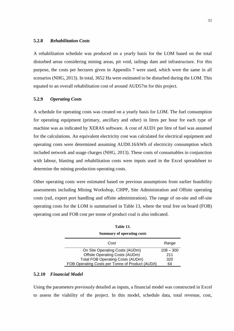
51
5.2.8 Rehabilitation Costs
A rehabilitation schedule was produced on a yearly basis for the LOM based on the total
disturbed areas considering mining areas, pit void, tailings dam and infrastructure. For this
purpose, the costs per hectares given in Appendix 7 were used, which were the same in all
scenarios (NHG, 2013). In total, 3652 Ha were estimated to be disturbed during the LOM. This
equated to an overall rehabilitation cost of around AUD57m for this project.
5.2.9 Operating Costs
A schedule for operating costs was created on a yearly basis for LOM. The fuel consumption
for operating equipment (primary, ancillary and other) in litres per hour for each type of
machine was as indicated by XERAS software. A cost of AUD1 per litre of fuel was assumed
for the calculations. An equivalent electricity cost was calculated for electrical equipment and
operating costs were determined assuming AUD0.16/kWh of electricity consumption which
included network and usage charges (NHG, 2013). These costs of consumables in conjunction
with labour, blasting and rehabilitation costs were inputs used in the Excel spreadsheet to
determine the mining production operating costs.
Other operating costs were estimated based on previous assumptions from earlier feasibility
assessments including Mining Workshop, CHPP, Site Administration and Offsite operating
costs (rail, export port handling and offsite administration). The range of on-site and off-site
operating costs for the LOM is summarised in Table 13, where the total free on board (FOB)
operating cost and FOB cost per tonne of product coal is also indicated.
Table 13.
Summary of operating costs
Cost Range
On Site Operating Costs (AUDm) 108 – 300 Offsite Operating Costs (AUDm) 211
Total FOB Operating Costs (AUDm) 320 FOB Operating Costs per Tonne of Product (AUD/t) 64
5.2.10 Financial Model
Using the parameters previously detailed as inputs, a financial model was constructed in Excel
to assess the viability of the project. In this model, schedule data, total revenue, cost,

52
depreciation and tax were included to develop the project cash flow. The project cash flow, Net
Present Value (NPV), internal rate of return (IRR) and cumulative profit/loss were calculated
for each scenario as a basis for comparison.
The project cash flow is the cumulative annual expenditure that will be needed for the LOM.
The smaller this value is the better. This means the company will need to spend less cash in
each year of the project life. The NPV shows the worth of the project at present taking into
account the time value of money. The more positive this value is the better. The NPV allows
comparing between different projects. The IRR shows the interest rate earned on the
investment. In practice, the IRR is the interest rate at which the NPV is equal to zero, but if all
cash flows are either positive or negative in a project, it cannot be calculated. The higher the
IRR the more attractive a project is. However, this parameter should not be analysed in isolation
but in conjunction with other metrics such as the NPV. The cumulative profit/loss is a measure
of how much money would be made (profits) after deducting the costs incurred (outgoings) to
earn such gain. The more positive this value is the better.
The key parameters that were defined for the financial model calculations were:
Discount rate of 10% (NHG, 2013);
Exchange rate of 0.75 AUD to USD (RBA, 2016);
Coal price of USD69.2/t of product based on Newcastle Standard (Indexmundi, 2016a);
Royalties based on revenue. If revenue was:
- Less than AUD100/t = 7%
- Between AUD100/t and AUD150/t = 12.5%
- Over AUD150/t = 15%;
Percentage of port cost deducted from royalty: 81.7%; and
100% equity.

53
RESULTS
6.1 PRELIMINARY RESULTS
6.1.1 Methodology Summary
Figure 26 summarises the methodology adopted to develop the models for each scenario. As
shown, the results from the three financial models created in this project were compared to the
2015 dragline values.
Figure 26. Simplified methodology model.
The key parameters that were defined to develop the three new models are summarised as
follows:
A target production rate of 5 Mtpa;
A stripping ratio cut-off of 7:1 was imposed;
Wombat coal price was energy adjusted to 92.1% of the Newcastle benchmark;
Only “Gold” quality product will be sold;
A salvage value of 10% of capital costs;
A roster of 2 x 12 hours shifts per day and 7 days per week for operation;
A cost of AUD1.00/L of fuel; and
A cost of AUD0.16/kWh of electricity, including network and usage charges.

54
The key parameters that were defined for the financial model calculations were:
Discount rate of 10% (NHG, 2013);
Exchange rate of 0.75 AUD to USD (RBA, 2016);
Coal price of USD69.2/t of product based on Newcastle Standard (Indexmundi, 2016a);
and
Royalties based on revenue. If revenue was:
- Less than AUD100/t = 7%
- Between AUD100/t and AUD150/t = 12.5%
- Over AUD150/t = 15%.
6.1.2 Infrastructure Capital and Equipment Costs Results
Table 14 shows the infrastructure capital for the three models built and the dragline. The cost
of the shovel was not included in either of the IPCC models because this was considered in the
equipment costs. The IPCC capital in Table 14 does not include the IPCC infrastructure cost
because the investment was incurred in year two of operation. The rope shovel required higher
capital than the face shovel due to its higher capacity. Table 14 also shows the initial investment
in equipment for each case at the start of the project. The face shovel IPCC had higher
equipment costs than the rope shovel because more excavators were needed to supplement the
smaller bucket capacity. Both IPCC models reduced the number of trucks as outlined in
Appendix 8.
Table 14.
Infrastructure and equipment capital costs
Case Infrastructure Capital (AUDm)
Equipment Costs (AUDm)
IPCC Face Shovel 727 203 IPCC Rope Shovel 727 180
Truck and Excavator 727 261 Dragline 640 224
6.1.3 Personnel Results
Using the estimated annual salaries, number of equipment and operating hours, the total number
of employees and cost of labour were calculated. Table 15 shows the average number of
employees per year as well as the average annual labour cost in each scenario.
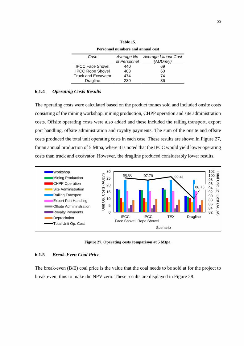
55
Table 15.
Personnel numbers and annual cost
Case Average No of Personnel
Average Labour Cost (AUDm/y)
IPCC Face Shovel 440 69 IPCC Rope Shovel 403 63
Truck and Excavator 474 74 Dragline 230 36
6.1.4 Operating Costs Results
The operating costs were calculated based on the product tonnes sold and included onsite costs
consisting of the mining workshop, mining production, CHPP operation and site administration
costs. Offsite operating costs were also added and these included the railing transport, export
port handling, offsite administration and royalty payments. The sum of the onsite and offsite
costs produced the total unit operating costs in each case. These results are shown in Figure 27,
for an annual production of 5 Mtpa, where it is noted that the IPCC would yield lower operating
costs than truck and excavator. However, the dragline produced considerably lower results.
Figure 27. Operating costs comparison at 5 Mtpa.
6.1.5 Break-Even Coal Price
The break-even (B/E) coal price is the value that the coal needs to be sold at for the project to
break even; thus to make the NPV zero. These results are displayed in Figure 28.
98.86 97.79 99.41
88.75
828486889092949698100102
0
5
10
15
20
25
30
IPCCFace Shovel
IPCCRope Shovel
TEX Dragline
To
tal U
nit O
p. C
ost (A
UD
/t)
Unit O
p.
Costs
(A
UD
/t)
Scenario
Workshop
Mining Production
CHPP Operation
Site Administration
Railing Transport
Export Port Handling
Offsite Admininstration
Royalty Payments
Depreciation
Total Unit Op. Cost
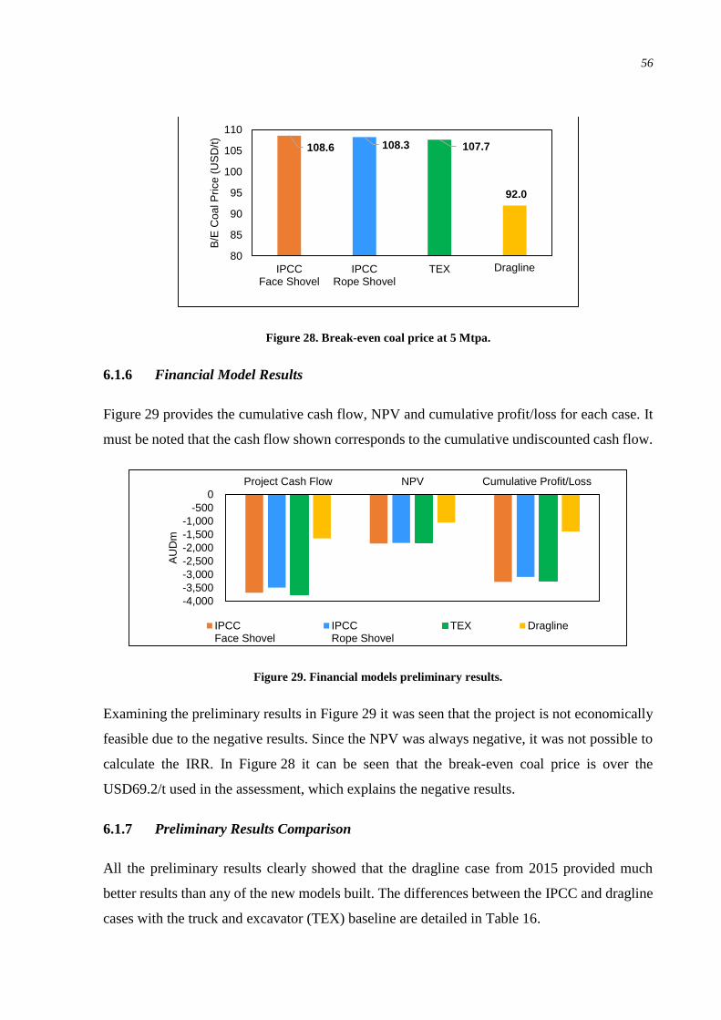
56
Figure 28. Break-even coal price at 5 Mtpa.
6.1.6 Financial Model Results
Figure 29 provides the cumulative cash flow, NPV and cumulative profit/loss for each case. It
must be noted that the cash flow shown corresponds to the cumulative undiscounted cash flow.
Figure 29. Financial models preliminary results.
Examining the preliminary results in Figure 29 it was seen that the project is not economically
feasible due to the negative results. Since the NPV was always negative, it was not possible to
calculate the IRR. In Figure 28 it can be seen that the break-even coal price is over the
USD69.2/t used in the assessment, which explains the negative results.
6.1.7 Preliminary Results Comparison
All the preliminary results clearly showed that the dragline case from 2015 provided much
better results than any of the new models built. The differences between the IPCC and dragline
cases with the truck and excavator (TEX) baseline are detailed in Table 16.
108.6 108.3 107.7
92.0
80
85
90
95
100
105
110
IPCCFace Shovel
IPCCRope Shovel
TEX RevisedDragline
B/E
Co
al P
rice
(U
SD
/t)
Dragline
-4,000
-3,500
-3,000
-2,500
-2,000
-1,500
-1,000
-500
0
Project Cash Flow NPV Cumulative Profit/Loss
AU
Dm
IPCCFace Shovel
IPCCRope Shovel
TEX Dragline
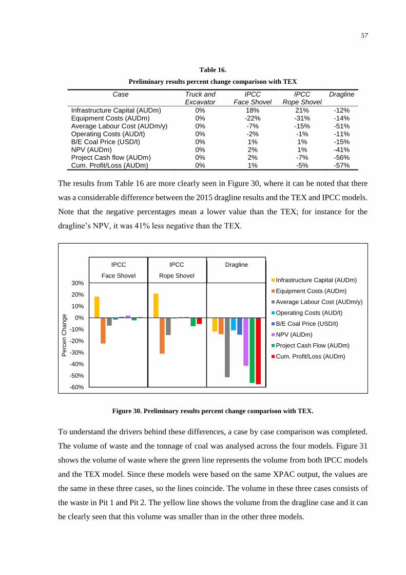
57
Table 16.
Preliminary results percent change comparison with TEX
Case Truck and Excavator
IPCC Face Shovel
IPCC Rope Shovel
Dragline
Infrastructure Capital (AUDm) 0% 18% 21% -12% Equipment Costs (AUDm) 0% -22% -31% -14% Average Labour Cost (AUDm/y) 0% -7% -15% -51% Operating Costs (AUD/t) 0% -2% -1% -11% B/E Coal Price (USD/t) 0% 1% 1% -15% NPV (AUDm) 0% 2% 1% -41% Project Cash flow (AUDm) 0% 2% -7% -56% Cum. Profit/Loss (AUDm) 0% 1% -5% -57%
The results from Table 16 are more clearly seen in Figure 30, where it can be noted that there
was a considerable difference between the 2015 dragline results and the TEX and IPCC models.
Note that the negative percentages mean a lower value than the TEX; for instance for the
dragline’s NPV, it was 41% less negative than the TEX.
Figure 30. Preliminary results percent change comparison with TEX.
To understand the drivers behind these differences, a case by case comparison was completed.
The volume of waste and the tonnage of coal was analysed across the four models. Figure 31
shows the volume of waste where the green line represents the volume from both IPCC models
and the TEX model. Since these models were based on the same XPAC output, the values are
the same in these three cases, so the lines coincide. The volume in these three cases consists of
the waste in Pit 1 and Pit 2. The yellow line shows the volume from the dragline case and it can
be clearly seen that this volume was smaller than in the other three models.
-60%
-50%
-40%
-30%
-20%
-10%
0%
10%
20%
30%
Face Shovel Rope Shovel
IPCC IPCC Dragline
Pe
rce
n C
ha
ng
e
Infrastructure Capital (AUDm)
Equipment Costs (AUDm)
Average Labour Cost (AUDm/y)
Operating Costs (AUD/t)
B/E Coal Price (USD/t)
NPV (AUDm)
Project Cash Flow (AUDm)
Cum. Profit/Loss (AUDm)

58
Figure 31. Comparison of waste volume across all cases.
Similarly, the tonnage of coal was also compared as shown in Figure 32 where it can be seen
that the dragline achieved the 5 Mtpa production target from the start of the project and finished
two years earlier, whereas the other three models considered a ramp-up in production.
Figure 32. Comparison of coal tonnage across all cases.
Based on this analysis it was concluded that the dragline model provided for comparison did
not include all the relevant results. It is probable that the truck and shovel components were not
included in the dragline model, which would explain the lower operating costs, or that the
volume from the smaller pit was also not provided, explaining the lower waste volumes. Since
the life of mine in the dragline case was two years shorter than in the new models built for this
project, the dragline model may have been optimised to reduce the mine life.
It was also found that the 2015 model considered the use of a second hand dragline, which
explains the lower capital costs and thus improved NPV, cash flow and cumulative profit/loss.
0
10
20
30
40
50
60
70
80
1 2 3 4 5 6 7 8 9 10 11 12 13 14 15 16 17 18 19 20 21 22 23 24 25 26 27 28 29 30
Waste
(M
bcm
)
Year
IPCC Face Shovel IPCC Rope Shovel TEX Dragline
0
1
2
3
4
5
6
1 2 3 4 5 6 7 8 9 10 11 12 13 14 15 16 17 18 19 20 21 22 23 24 25 26 27 28 29 30
Coa
l (M
t))
Year
IPCC Face Shovel IPCC Rope Shovel TEX Dragline
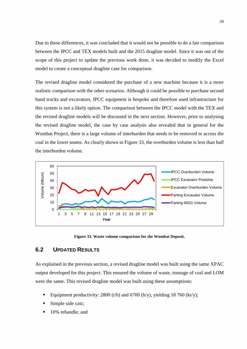
59
Due to these differences, it was concluded that it would not be possible to do a fair comparison
between the IPCC and TEX models built and the 2015 dragline model. Since it was out of the
scope of this project to update the previous work done, it was decided to modify the Excel
model to create a conceptual dragline case for comparison.
The revised dragline model considered the purchase of a new machine because it is a more
realistic comparison with the other scenarios. Although it could be possible to purchase second
hand trucks and excavators, IPCC equipment is bespoke and therefore used infrastructure for
this system is not a likely option. The comparison between the IPCC model with the TEX and
the revised dragline models will be discussed in the next section. However, prior to analysing
the revised dragline model, the case by case analysis also revealed that in general for the
Wombat Project, there is a large volume of interburden that needs to be removed to access the
coal in the lower seams. As clearly shown in Figure 33, the overburden volume is less than half
the interburden volume.
Figure 33. Waste volume comparison for the Wombat Deposit.
6.2 UPDATED RESULTS
As explained in the previous section, a revised dragline model was built using the same XPAC
output developed for this project. This ensured the volume of waste, tonnage of coal and LOM
were the same. This revised dragline model was built using these assumptions:
Equipment productivity: 2800 (t/h) and 6700 (h/y), yielding 18 760 (kt/y);
Simple side cast;
10% rehandle; and
0
10
20
30
40
50
60
1 3 5 7 9 11 13 15 17 19 21 23 25 27 29
Vo
lum
e (
Mb
cm
)
Year
IPCC Overburden Volume
IPCC Excavator Poststrip
Excavator Overburden Volume
Parting Excavator Volume
Parting 992G Volume

60
1 dozer needed.
The simplified methodology model in Figure 26 (Section 6.1.1) was modified as shown in
Figure 34.
Figure 34. Revised methodology model.
6.2.1 Revised Dragline Model Results
Tables 17 and 18 show the updated results for the revised dragline model including
infrastructure and equipment capital, as well as personnel needs and costs. Figure 35 displays
the updated operating costs.
Table 17.
Updated infrastructure and equipment capital costs
Case Infrastructure Capital (AUDm)
Equipment Costs (AUDm)
IPCC Face Shovel 727 203 IPCC Rope Shovel 727 180
Truck and Excavator 727 261 Revised Dragline 727 283
Table 18.
Updated personnel numbers and annual cost
Case Average No of Personnel
Average Labour Cost (AUDm/y)
IPCC Face Shovel 440 69 IPCC Rope Shovel 403 63
Truck and Excavator 474 74 Revised Dragline 390 61

61
Figure 35. Updated operating costs comparison at 5 Mtpa.
These results show that the revised dragline model was similar to the other three models, and
therefore a comparison was realistic. Examining the operating costs in more detail, as seen in
Figure 36, almost half of these costs are from railing transport, and almost a third from export
port handling. These are fixed costs that account for almost 50% of the total operating costs in
all models.
Figure 36. Fixed operating costs.
Figures 37 and 38 provide the updated break-even coal price and the results from the financial
model. These figures show that the revised dragline model was closer to the other cases, which
is confirmed in Table 19 and Figure 39. It should be noted that for purpose of comparison, the
IPCC infrastructure capital shown in Table 19 and Figure 39 included the full costs for the
system. This means that the IPCC capital delayed to year 2 was included in the results to allow
a fair comparison. This only applied to Table 19 and Figure 39 results. Figure 38 shows that the
project was not economically feasible in any of the scenarios assessed.
98.8697.79
99.41
97.46
96
97
97
98
98
99
99
100
100
0
5
10
15
20
25
30
IPCCFace Shovel
IPCCRope Shovel
TEX RevisedDragline
To
tal U
nit O
p. C
ost (A
UD
/t)
Un
it O
p.
Co
sts
(A
UD
/t)
Workshop
Mining Production
CHPP Operation
Site Administration
Railing Transport
Export Port Handling
Offsite Admininstration
Royalty Payments
Depreciation
Total Unit Op. Cost
14%
44%
28%
5%
9%
Site Admin.
Railing Transport
Export Port Handling
Offsite Admin.
Royalty Payments

62
Figure 37. Updated break-even coal price.
Figure 38. Updated financial model results.
Table 19.
Percent change comparison with TEX for updated results
Case Truck and Excavator
IPCC IPCC Revised Dragline Face
Shovel Rope
Shovel
Infrastructure Capital (AUDm) 0% 18% 21% 0%
Equipment Costs (AUDm) 0% -22% -31% 8%
Average Labour Cost (AUDm/y) 0% -7% -15% -18%
Operating Costs (AUD/t) 0% -2% -1% -2%
B/E Coal Price (USD/t) 0% 1% 1% 0%
NPV (AUDm) 0% 2% 1% 0%
Project Cash Flow (AUDm) 0% -2% -7% -7%
Cum. Profit/Loss (AUDm) 0% 1% -5% -4%
108.6 108.3
107.7 107.8
107
108
109
IPCCFace Shovel
IPCCRope Shovel
TEX RevisedDragline
B/E
Co
al P
rice
(U
SD
/t)
-4,000
-3,500
-3,000
-2,500
-2,000
-1,500
-1,000
-500
0
Project Cash Flow NPV Cumulative Profit/Loss
AU
Dm
IPCCFace Shovel
IPCCRope Shovel
TEX RevisedDragline

63
Figure 39. Updated results percent change comparison with TEX.
Although the revised dragline model produced results that were comparable with the other three
models, the revised dragline produced most favourable values in comparison with the TEX.
Delaying the implementation of the IPCC improved the equipment capital in year 1 and the
NPV for both models, however the total infrastructure costs were still higher compared to the
revised dragline and TEX.
Similarly, the revised dragline improved the NPV by making it slightly less negative (smaller
negative value) than the TEX, while both IPCC’s values were worse than the TEX. Comparing
between the IPCC scenarios, the rope shovel produced better results than the face shovel, at a
5 Mtpa production rate.
6.2.2 Sensitivity Analysis
A sensitivity analysis for each model was also completed, as detailed in Figures 40 to 43. The
most sensitive parameters were the cash cost free on board (FOB) and the coal price. The coal
price referred to the selling price for product coal. The cash cost FOB was inversely
proportional to the NPV meaning that an increase in this cost would result in a reduced NPV.
These costs depended on the operating costs and in all cases, the operating costs were the next
most sensitive inversely proportional variable affecting the NPV followed by capital.
-40%
-30%
-20%
-10%
0%
10%
20%
30%
Face Shovel Rope Shovel
IPCC IPCC New Dragline
Pe
rce
n C
ha
ng
e
Infrastructure Capital (AUDm)
Equipment Costs (AUDm)
Average Labour Cost (AUDm/y)
Operating Costs (AUD/t)
B/E Coal Price (USD/t)
NPV (AUDm)
Project Cash Flow (AUDm)
Cum. Profit/Loss (AUDm)
Revised
Dragline

64
The coal price and the revenue line coincided in the sensitivity graphs, because they were
directly proportional. An increase in the coal price would improve the results, because this had
a direct impact on the yearly revenues; thus at a higher coal price the NPV is better.
Figure 40. Sensitivity analysis IPCC face shovel.
Figure 41. Sensitivity analysis IPCC rope shovel.
-3,500
-3,000
-2,500
-2,000
-1,500
-1,000
-500
0
-30 -20 -10 0 10 20 30
NP
V (
AU
Dm
)
% Change
Coal Price
Electricity
Fuel
Discount Rate
Capital
Operating Costs
Revenue
Labour Cost
Cash Cost (FOB)
-3,500
-3,000
-2,500
-2,000
-1,500
-1,000
-500
0
-30 -20 -10 0 10 20 30
NP
V (
AU
Dm
)
% Change
Coal Price
Electricity
Fuel
Discount Rate
Capital
Operating Costs
Revenue
Labour Cost
Cash Cost (FOB)

65
Figure 42. Sensitivity analysis TEX.
Figure 43. Sensitivity analysis revised dragline.
Having a closer look at the capital, labour and electricity costs, Figures 44 to 47 display a
comparison of these results across the four cases. In Figure 44 it can be seen that the sensitivity
of capital costs was similar in all models but the revised dragline was slightly better because it
was less negative than the other scenarios. This similarity was also due to the delay in the
implementation of the IPCC, which reduced the capital in year 1 of the project.
-3,500
-3,000
-2,500
-2,000
-1,500
-1,000
-500
0
-30 -20 -10 0 10 20 30
NP
V (
AU
Dm
)
% Change
Coal Price
Electricity
Fuel
Discount Rate
Capital
Operating Costs
Revenue
Labour Cost
Cash Cost (FOB)
-3,500
-3,000
-2,500
-2,000
-1,500
-1,000
-500
0
-30 -20 -10 0 10 20 30
NP
V (
AU
Dm
)
% Change
Coal Price
Electricity
Fuel
Discount Rate
Capital
Operating Costs
Revenue
Labour Cost
Cash Cost (FOB)

66
Figure 44. Sensitivity comparison capital costs.
Figure 45 shows the sensitivity of labour costs and it can be observed that all cases were similar.
However, the revised dragline case was slightly less sensitive than the other three models. This
is explained in Figure 46 where it is noted that the revised dragline required slightly less
employees than the other models early in the life of the project and most of the LOM.
Figure 45. Sensitivity comparison labour costs.
-3,000
-2,000
-1,000
-30 -20 -10 0 10 20 30N
PV
(A
UD
m)
% Change
IPCC Face Shovel IPCC Rope Shovel TEX Revised Dragline
-3,000
-2,000
-1,000
-30 -20 -10 0 10 20 30
NP
V (
AU
Dm
)
% Change
IPCC Face Shovel IPCC Rope Shovel TEX Revised Dragline

67
Figure 46. Comparison of labour requirements.
Comparing the electricity costs, as shown in Figure 47 the revised dragline and TEX were rather
unaffected by changes in this variable, however the dragline’s results were much better than the
other scenarios. This was due to the assumptions made for the equipment, which were the same
as in the 2015 study. The rope shovel was less sensitive to changes in the electricity costs than
the face shovel. This is because, although the face shovel is smaller than the rope shovel, it
required more electricity to power the hydraulic systems. Recall that the shovel to load the IPCC
in each case was an electrically driven machine.
Figure 47. Sensitivity comparison electricity.
6.2.3 Financing Options for IPCC Infrastructure
Since both IPCC cases did not improve the NPV in comparison with the TEX scenario, it was
decided to investigate financing the IPCC infrastructure. This means incurring a debt to
0
100
200
300
400
500
600
1 2 3 4 5 6 7 8 9 10 11 12 13 14 15 16 17 18 19 20 21 22 23 24 25 26 27 28 29 30
No
of E
mp
loye
es
Year
IPCC Face Shovel IPCC Rope Shovel TEX Revised Dragline
-1,900
-1,850
-1,800
-1,750
-1,700
-1,650
-30 -20 -10 0 10 20 30
NP
V (
AU
Dm
)
% Change
IPCC Face Shovel IPCC Rope Shovel TEX Revised Dragline

68
purchase all the equipment for the in-pit crushing system except the shovel. Based on the
Client’s advice, financing was analysed for both IPCC cases using these assumptions:
Repayment period of 15 years; and
Annual interest over debt of 7%.
Figure 48 shows the comparison of results from the financial models in each IPCC case, where
it is seen that financing the infrastructure would improve the NPV in both scenarios, as well as
the profit over losses. However, the cumulative cash flow and profit/loss was worse due to debt
repayments.
Figure 48. Comparison of financed IPCC models.
Table 20 details the percent change when financing each IPCC system compared to not
financing the infrastructure. In Table 20 a positive percentage represents a less favourable result
because it is a more negative value, while a negative percentage has the opposite effect with the
values being less negative (a smaller negative number).
Table 20.
Percent change results for financed IPCC infrastructure
Case IPCC Face Shovel
Financed IPCC Rope Shovel
Financed
Project Cash Flow (AUDm) 2% 3%
NPV (AUDm) -1% -1%
Cum. Profit/Loss (AUDm) -4% -4%
The results from the financed IPCC models and the revised dragline were compared to the TEX,
as shown in Figure 49. The NPV for the financed face shovel IPCC improved to 1% more
-3,770
-1,829
-3,167
-3,594
-1,807
-2,958
-4,000
-3,000
-2,000
-1,000
0
Project Cash Flow NPV Cumulative Profit/Loss
AU
Dm
IPCCFace Shovel
IPCC Fin.Face Shovel
IPCCRope Shovel
IPCC Fin.Rope Shovel

69
negative from the 2% without financing. The project cash flow became more negative than the
TEX. The cumulative profit loss improved from 1% more negative to 3% less negative than the
TEX. For the rope shovel arrangement, the NPV improved from 1% more negative to 0.1% less
negative than the TEX, bringing this result closer to the revised dragline scenario. The project
cash flow changed from -7% to -5% less negative than the TEX while the cumulative profit/loss
did not change. Figure 49 clearly shows that the financed rope shovel IPCC produced the best
results; however the dragline was still better than both IPCCs compared to the TEX.
Figure 49. Financed IPCC and dragline results compared to TEX.
6.3 RESULTS AT USD120/T
Both financed IPCC, the revised dragline and TEX financial models were re-assessed at a coal
price of USD120/t as this allowed comparison with the 5 Mtpa Truck and Shovel (T&S) results
from 2013. Figure 50 shows the results from this analysis, where for simplicity, only the NPV
and IRR are shown.
-10%
-8%
-6%
-4%
-2%
0%
2%
Face Shovel Rope Shovel
IPCC Fin. IPCC Fin. Revised Dragline
Pe
rce
n C
ha
ng
e
NPV (AUDm)
Project Cash Flow (AUDm)
Cum. Profit/Loss (AUDm)
Revised
Dragline

70
Figure 50. NPV and IRR comparison at 120 USD/t.
It is evident from Figure 50 that the new models produced improved results in comparison to
the 2013 truck and shovel case. This was due to the increased reserves and extended LOM that
the new models yielded; 150 Mt compared to 82 Mt and 30 years as opposed to 17 years
respectively. The revised dragline model produced better results at a coal price of USD120/t,
however at this price, the TEX was better than both IPCC because the break-even coal price for
this model was lower. These results are detailed in Table 21.
Table 21.
NPV and IRR results at USD120/t
Case IPCC Face Shovel
Financed IPCC Rope
Shovel Financed TEX
Revised Dragline
T&S
NPV (AUDm) 420 432 454 515 95
IRR (%) 16% 16% 16% 17% 12%
In spite of the improved results with a dragline, the IPCC with a rope shovel was better than the
face shovel case.
6.4 PROJECT RISKS
Although the results showed that the revised dragline provided better outcomes, it is necessary
to consider the risks of each option. Conducting a full risk assessment is beyond the scope of
this research project; however, some key factors are discussed in the next subsections.
16% 16% 16% 17%
12%
0%
2%
4%
6%
8%
10%
12%
14%
16%
18%
0
100
200
300
400
500
600
IPCC Fin.(R9800)
IPCC(CAT7495)
TEX RevisedDragline
T&S
IRR
(%)
NP
V (
AU
Dm
)
IRR

71
6.4.1 Operational Risks
Truck and shovel operations provide increased flexibility to implement short-term changes to
the mine plan should market conditions change. Both IPCC and dragline systems are inflexible
in this regard and once either of these systems has been selected, changes to short-term planning
will be hard to implement due to the equipment size and layout needs.
The truck and shovel method is also more commonly used in Australian mines and the
equipment is transferable between different sites. Since shovels have shorter lives than
draglines or IPCC, it is likely that the equipment be sold in case of unfavourable economic
conditions. Draglines and IPCC are bespoke systems and thus re-selling this equipment is not
guaranteed. They also require large annual throughputs to function economically but they
cannot be easily upgraded if an increased production rate is needed, whereas it is easier to
purchase additional trucks and shovels for these needs.
IPCC systems are exposed to a higher risk of downturns from equipment reliability than truck
and shovel because if a component breaks down, the whole system stops. In truck and shovel
methods, it is possible to have spare capacity to overcome these problems.
IPCC rely on the use of conveyors to replace the trucks. Since this is a continuous operation
there are risks associated with moving plant, especially conveyor rollers which can lead to fires,
particularly when coal accumulates under the belt. The constant operation of the conveying
system also produces vibrations that may affect the integrity of the support structures over time.
This may require increased needs for condition monitoring than with other methods, which is
an added costs to the operation.
In spite of the negative aspects of draglines and IPCC, these systems did provide lower
operating costs. As shown in Section 6.2.1, the operating costs directly impacted the total cash
FOB costs and thus these methods are less risky from an operating cost perspective. IPCC
systems use a more steady supply of electricity than draglines avoiding the peaks and troughs
when the machine is digging. IPCCs power demand fluctuates less than draglines and thus there
are less risks of impacting operations due to outages.

72
IPCC systems are less affected by weather events that will stop trucks; namely fog and heavy
rainfall. IPCC also require less maintenance of haul roads than trucks, and conveyors can
traverse higher grades than tucks.
6.4.2 Financial Risks
Since IPCC and draglines are less flexible to market conditions, they are at higher risks than
truck and shovel. The sensitivity analysis showed that the revenue, directly dependant on the
coal price, was one of the most sensitive variables affecting the NPV. In the current market, the
volatility of the coal price could have devastating effects on a dragline or IPCC operation.
However, since draglines are not totally bespoke (some but not all components are), they are at
lower risk than an IPCC method because a dragline could potentially be re-purposed for another
operation by modifying part of its components. Draglines are also commonly used in other
Queensland mines, whereas IPCC is not employed extensively at present.
6.4.3 Environmental and Social Risks
Truck and shovel methods produce higher dust and CO2 emissions than IPCC systems. Since
IPCC reduces the number of trucks, less water is needed to maintain haul roads, also reducing
dust generation. However, due to the size of the IPCC infrastructure, transport to site and
installation may be more disruptive than in a truck and shovel case, which also increases the
risk of negatively affecting local communities although temporarily.
6.4.4 Health and Safety Risks
All the mining methods examined require the operators to work in the pit; however IPCC
reduced the number of trucks needed for haulage and thus the number of people working at the
active face. In the IPCC working area there is no need for trucks, therefore there is a reduced
risk of vehicle interaction and risks associated to trucks operation such as trucks catching fire.

73
CONCLUSIONS
This project examined the use of a continuous mining system at a concept level for the Wombat
deposit. A BWE and IPCC were evaluated and the geotechnical conditions assessment showed
the strata will require blasting to improve excavation. Thus, it would not be possible to free-dig
using a BWE. The study then focused on implementing an IPCC considering the suitable
mining horizons, a proposed system layout and a target production of 5 Mtpa of thermal coal.
The Wombat Project was analysed in the past using truck and shovel in 2013 and a dragline in
2015. Current market conditions made the project not economically feasible. Thus, an IPCC
was analysed with the expectation of reducing operating costs and improving the economic
benefits of the project. In this study, initially three models were developed; an IPCC with a
large shovel, an IPCC with a smaller face shovel and a truck and excavator case (TEX) as a
baseline for comparison. These three models were compared with the dragline case. The new
models showed the project had a life of 30 years and 150 Mt reserves.
This analysis also showed that the 2015 dragline model supplied did not include all relevant
information to guarantee a realistic comparison. Hence, a revised dragline model was built
based on the new models generated in this study. At a coal price of USD69.2/t, current at the
time of the assessment, it was found that the project was not economically feasible. The IPCC
did reduce the operating costs due to less number of operators needed than the TEX case and
less number of trucks. However the dragline provided better results than both IPCC scenarios.
Further assessment demonstrated that financing the IPCC infrastructure improved the results
with respect to TEX. The NPV for the IPCC face shovel case improved from 2 to 1% less
negative and the rope shovel improved from 1% more negative to 0% compared to the TEX,
which was similar to the dragline. Nevertheless, the dragline provided considerably better cash
flow and profit loss (7 and 9% less negative respectively) than the TEX. This was better than
both IPCC models. The rope shovel proved the best of the IPCC scenarios. All scenarios were
within a ± 30% margin which was expected at a concept study level.
A final comparison was carried out at a coal price of USD120/t between the TEX, financed
IPCC, revised dragline and the truck and shovel cases. This clearly showed that the new models
produced improved results over the truck and shovel study from 2013, due to increased reserves

74
and longer mine life. The revised dragline model still produced the best results, however at the
higher coal price, the TEX was better than both IPCC models. This was due to the lower break-
even coal price of the TEX model. The rope shovel was also the best IPCC option.
Although the assessment suggested that a dragline would optimise the results at a 5 Mtpa
production rate, the risks related to each method must be considered. The risks for an IPCC
system were identified, and the key factors are summarised in Figure 51, where they have been
grouped as strengths, weaknesses, opportunities and threats (SWOT).
Strengths Opportunities
Reduces operating costs Less susceptible to weather conditions than
other methods
Innovative method in Queensland coal mines Reduces CO2 and dust emissions
Weaknesses Threats
Difficult to modify short-term planning to adjust to market conditions
Method is not commonly used in Queensland
High capital and low flexibility make it a risky investment in changing market conditions
Reliability of individual components can disrupt continuous operation
Figure 51. SWOT for IPCC risks.
In addition to the SWOT analysis of IPCC risks, it must be emphasised that the results were
achieved imposing a target of production of 5 Mtpa, which may not be the optimum output for
the IPCC. An alternative approach to conduct this research could also have yielded different
results. For instance, the research could have focused only on analysing the IPCC to determine
the optimum working conditions first, including the preferred target production and size of the
primary loading equipment, and then creating the other models for comparison based on the
IPCC needs. This would have simplified the analysis, in particular the comparison of all cases.
In spite of the differences between all the scenarios, one common factor that influenced the
results was the large volume of interburden that currently needs to be removed with excavators,
as well as the fixed operating costs. These two factors offset the results across all cases.
In conclusion, after modelling and comparing the different scenarios, the results suggested that
a dragline would be most suitable for this deposit. However, since the studies were carried out
at a concept level for a particular mining production, the answer is not definitive and further
assessment as well as research needs to be conducted for this project.

75
RECOMMENDATIONS
Judging by the results of the different scenarios analysed and considering the conclusions drawn
in this study, several recommendations can be made to improve this research work:
Run the IPCC models at higher production targets. This was done in the previous
assessments and since IPCC requires high throughput, this could improve the results for
the system.
Investigate different financing options for IPCC infrastructure since this study
demonstrated that the results improved in this case.
Analyse the cost of overburden removal only between IPCC and the other methods. This
is the cost per bcm of waste. If the IPCC is found to be more cost effective, it would
justify investigating the use of an IPCC system at deeper horizons, which would require
a higher level of technical analysis.
Investigate a method to optimise the interburden removal. For instance using a surface
miner, which was analysed in 2014, when it was suggested this machine could be
optimised in combination with a conveyor based transport system. Another alternative
is to optimise interburden removal using specialised software such as TALPAC.
Explore optimising Pit 2 mining, required for tailings storage. This could also be done
through TALPAC or assessing the use of contractors.
Conduct a full risk assessment for a dragline and an IPCC, and establish the impact of
using these methods on the current mine plan, especially key infrastructure such as the
CHPP, and project approvals including the EIS for increased throughputs.
Verify and update the assumptions used, especially those related to fixed operating costs
because they had a considerable impact on the results.
Quantify the impact of the Surat Rail link on this project and incorporate this into the
analysis. All previous assessment and this study have not included this cost. However,
the project depends entirely on this infrastructure being built. This will impact the
implementation of this project independently of the mining method used.
Consolidate all different scenarios analysed into a single project base to ensure the
assumptions and inputs are the same throughout all models. This will ease the
comparison of the scenarios with new conditions (eg. coal price).

76
REFERENCES
Aiken, G E and Gunnett, J W, 1990. Overburden removal, in Surface Mining, (ed: B A,
Kennedy), pp 584-657 (Society for Mining, Metallurgy and Exploration: Littleton).
Atchison, T and Morrison, D, 2011. In-pit crushing and conveying bench operations, in
Proceedings of Iron Ore Conference, Perth, Australia, pp 157-163 (The Australasian
Institute of Mining and Metallurgy).
Australian Government, Bureau of Resources and Energy Economics, 2012. Australian bulk
commodity exports and infrastructure-outlook to 2025 [online]. Available from:
<http://industry.gov.au/Office-of-the-Chief-
Economist/Publications/Documents/other/export-infrastructure-report.pdf>
[Accessed: 1 May 2016].
Blunck, S, 2016. Personal communication, 25 July. Regional Manager, RWE Australia.
Blunck, S, 2016a. Personal communication, 9 August. Regional Manager, RWE Australia.
Cooney, J, 2016. Personal communication, 10 March. Business Analyst, New Hope Group.
Cooney, J, 2016a. Personal communication, 4 April. Business Analyst, New Hope Group.
Cooney, J, 2016b. Personal communication, 11 April. Business Analyst, New Hope Group.
Cooney, J, 2016c. Personal communication, 11 May. Business Analyst, New Hope Group.
Cooney, J, 2016d. Personal communication, 29 June. Business Analyst, New Hope Group.
Cooney, J, 2015. Conveyor mining systems and application to a Queensland coal mine.
Presentation delivered at New Hope Group Corporate Office, Brookwater, 27 October.
Darling, P, 2015. Bucket wheel excavators: dutiful and versatile giants of the mining industry
[online]. Coal International, 263(3), 22-27. Available from:
<http://connection.ebscohost.com> [Accessed: 27 March 2016].

77
Darling, P, 2015a. In-pit crushing-and-conveying: enjoying a new lease of life? [online]. Coal
International, 263(2), 30-35. Available from: <http://connection.ebscohost.com>
[Accessed: 08 April 2016].
Dyer, G and Hill, K, 2011. Strip mining, in SME Mining Engineering Handbook (ed: P Darling),
pp 990-996 (Society for Mining, Metallurgy and Exploration: Littleton).
Hagemann, 2014a. Newstan coal mine put back into care and maintenance [online]. Available
from: <https://australianmining.com.au/news/> [Accessed: 1 May 2016].
Hagemann, 2014b. Peabody to strip Queensland assets [online]. Available from:
<https://australianmining.com.au/news/> [Accessed: 1 May 2016].
Hartman, H L and Mutmansky, J M, 2002. Introductory Mining Engineering, pp 138-142, 197-
204 (John Wiley: Hoboken).
Humphrey, D and Wagner, D, 2011. Mechanical extraction, loading, and hauling, in SME
Mining Engineering Handbook (ed: P Darling), pp 903-929 (Society for Mining,
Metallurgy and Exploration: Littleton).
Indexmundi, 2016. Coal, Australian thermal coal monthly price - Australian Dollar per metric
ton [online]. Available from: <http://www.indexmundi.com/> [Accessed: 8 April
2016].
Indexmundi, 2016a. Coal, Australian thermal coal monthly price - Australian Dollar per metric
ton [online]. Available from: <http://www.indexmundi.com/> [Accessed: 20 July
2016].
Insite Geology, 2010. Wombat coal project Southern Queensland additional report on
geotechnical conditions (unpublished).
Insite Geology, 2009. Wombat coal project Southern Queensland report on assessment of
geotechnical conditions (unpublished).
Knowledge Infrastructure Systems, 2016. Coal energy calculator [online]. Available from:
<http://www.knowledgeispower.in/calculator.asp> [Accessed: 15 August 2016].

78
Metso, 2015. In-pit crushing and conveying IPCC solutions from Metso [online]. Available
from: <http://www.metso.com/miningandconstruction/> [Accessed: 1 May 2016].
Minerals Council of Australia, 2016. Characteristics of the Australian coal industry [online].
Available from: <http://www.minerals.org.au/> [Accessed: 1 May 2016].
New Hope Group (NHG), 2016. About us [online]. Available from:
<http://www.newhopegroup.com.au/> [Accessed: 16 March 2016].
New Hope Group (NHG), 2015. JORC report Wombat reserves (unpublished).
New Hope Group (NHG), 2013. Wombat Project mine plan review (unpublished).
New Hope Group (NHG), 2009. New Acland coal mine stage 3 expansion project
environmental impact statement [online]. Available from:
<http://www.newhopegroup.com.au/files/files/projects/acland2009> [Accessed: 14
May 2016].
Potter, B, 2015. Australia's coal exports set to rise as South-East Asia demand surges, Financial
Review [online]. Available from: <http://www.afr.com/business/mining/coal/>
[Accessed: 1 May 2016].
Queensland Government, 2016. MinesOnlineMaps Mobile [online]. Available from:
<https://minesonlinemaps.business.qld.gov.au> [Accessed: 20 March 2016].
Queensland Government, 2010. Coal plan 2030 [online]. Available from:
<http://www.statedevelopment.qld.gov.au/resources/plan/cg/coal-plan-2030.pdf>
[Accessed: 26 March 2016].
Reserve Bank of Australia (RBA), 2016. Exchange rates [online]. Available from:
<http://www.rba.gov.au/statistics/frequency/exchange-rates.html> [Accessed: 20 July
2016].
Rokovic, A, 2016. Personal Communication, 22 August. Account Manager, Thyssen Krupp
Industrial Solutions.

79
Sandvik, 2008. In-pit crushing and conveying-IPCC [online]. Available from:
<http://www.miningandconstruction.sandvik.com/> [Accessed: 8 April 2016].
Saunders, A, 2014. Anglo American boss sees coal mines closing at a rate of one a fortnight,
The Sydney Morning Herald [online]. Available from:
<http://www.smh.com.au/business/mining-and-resources/> [Accessed: 1 May 2016].
Schroeder, D and Schwier, U, 1995. Selection of Mining Systems for Large Open Pits. Surface
Mining, 48 (1995), No 5, September/October, pp 479-486.
Schroeder, D, 1994. Technical and economical aspects of continuous mining with bucket wheel
excavators. Zement-Kalk-Gips, No 9/1994, pp 513-518.
Schroder, D, 1993. Bucket wheel excavators for semi-hard rock as an alternative to blasting.
ZKG International, re-print from issue No 8 of 1993.
Seib, W, 2016. Personal communication, 27 July. Independent Consultant and Adjunct
Professor/Senior Industry Teaching Fellow Department of Mining, The University of
Queensland.
Smith, E, 2015. Abbot Point 'facilitating growth on back of demand’, Daily Mercury [online].
Available from: <http://www.dailymercury.com.au/news/> [Accessed: 1 May 2016].
Tenova, 2013. Bucket wheel excavators [online]. Available from:
<http://www.takraf.com/en/Products/Mining_Equipments/bucketwheelexcavator.htm
> [Accessed: 26 March 2016].
Turnbull, D and Cooper, A, 2009. In-pit crushing and conveying (IPCC) – a tried and tested
alternative to trucks, in Proceedings of The AusIMM New Leaders’ Conference,
Brisbane, Australia, pp 59-66 (The Australasian Institute of Mining and Metallurgy).
Uren, A, 2014. Implications of using a surface miner for coal mining and parting removal in
the Wombat Mine, Bachelor of Engineering Thesis (unpublished), The University of
Queensland, Brisbane.
Utley, R W, 2011. In-pit crushing, in SME Mining Engineering Handbook (ed: P Darling), pp
941-956 (Society for Mining, Metallurgy and Exploration: Littleton).

80
Wilson, G, 2015. Establishing the viability of using a surface miner with a dragline and bulk
dozer push at the Wombat Mine, Bachelor of Engineering Thesis (unpublished), The
University of Queensland, Brisbane.
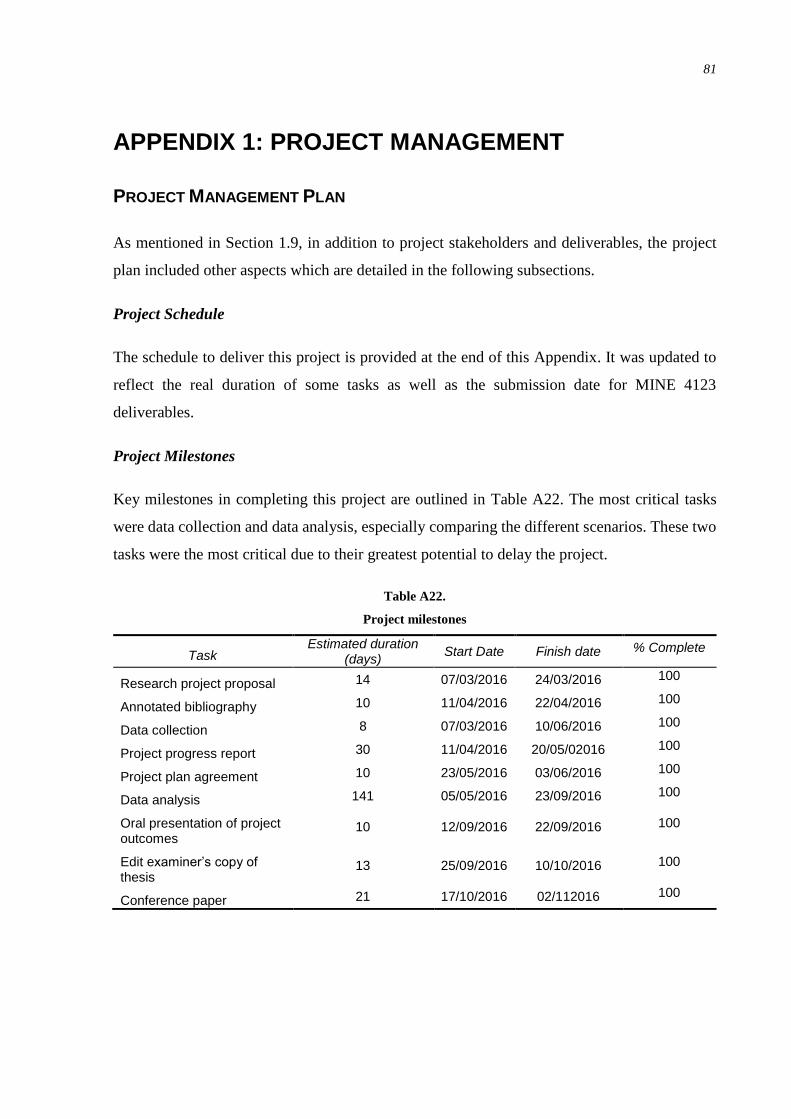
81
APPENDIX 1: PROJECT MANAGEMENT
PROJECT MANAGEMENT PLAN
As mentioned in Section 1.9, in addition to project stakeholders and deliverables, the project
plan included other aspects which are detailed in the following subsections.
Project Schedule
The schedule to deliver this project is provided at the end of this Appendix. It was updated to
reflect the real duration of some tasks as well as the submission date for MINE 4123
deliverables.
Project Milestones
Key milestones in completing this project are outlined in Table A22. The most critical tasks
were data collection and data analysis, especially comparing the different scenarios. These two
tasks were the most critical due to their greatest potential to delay the project.
Table A22.
Project milestones
Task Estimated duration
(days) Start Date Finish date % Complete
Research project proposal 14 07/03/2016 24/03/2016 100
Annotated bibliography 10 11/04/2016 22/04/2016 100
Data collection 8 07/03/2016 10/06/2016 100
Project progress report 30 11/04/2016 20/05/02016 100
Project plan agreement 10 23/05/2016 03/06/2016 100
Data analysis 141 05/05/2016 23/09/2016 100
Oral presentation of project outcomes
10 12/09/2016 22/09/2016 100
Edit examiner’s copy of thesis
13 25/09/2016 10/10/2016 100
Conference paper 21 17/10/2016 02/112016 100

82
Project Related Resources
To complete the project, it was necessary to have access to the following resources:
Access to NHG office and databases.
Microsoft Office software: Word, Excel. Powerpoint and Project.
Specialised software; Minescape and XPAC.
Project specific files; geological model and project plan.
Project costing data; capital and operating expenditure, unit costs and closure costs.
Client and Project Sponsor availability.
Consumables (stationery, computer, petrol and printing products).
Project Related Budget
Project costs were estimated as detailed in Table A2.
Table A2.
Project cost estimation
Expense Rate (AUD/h) Hours (h) Total (AUD)
Travel to/from office 40 18 720 Consultation with Client 100 56 5600 Project Sponsor consultation 120 30 3600 Project management 80 80 6400 Consumables (* lump sum) 800* - 800 Total (AUD) 17 120
Project Delivery Risk Assessment
The contingency plan outlined in Section 1.9 was defined using the risk ranking matrix shown
in Figure A1.

83
Figure A1. NHG risk ranking matrix
(NHG, 2009).
The main constraint for completing the project was time; thus the consequence and likelihood
in Figure A1 were defined in Table A3 and Table A4 respectively.
Table A3.
Risk matrix consequence definition
Rank Consequence Definition
1 Catastrophic Irreversible detrimental effect on time loss. The project is delayed past the due date for completion and minimum quality standard is not achieved
2 Major Prolonged but reversible effect on time loss. The project is completed after the deadline to a low quality
3 Moderate Short term detrimental effect on time loss. The project is completed within the deadline but to a lower quality
4 Minor Minor short term detrimental effect on time loss. The project is completed within the deadline but with minor loss of quality
5 Insignificant No detrimental effect on time loss. Quality is preserved.
Table A4.
Risk matrix likelihood definition
Rank Likelihood Definition
A Almost certain
The event is expected to occur in most circumstances (at least once per week)
B Likely The event will probably occur in most circumstances (at least ten times per year) C Possible The event could possibly occur at some time (at least twice per year) D Unlikely The event could possibly occur at some time but is unlikely (at least once per
year) E Rare The event may occur only in exceptional circumstances (less than once per year)
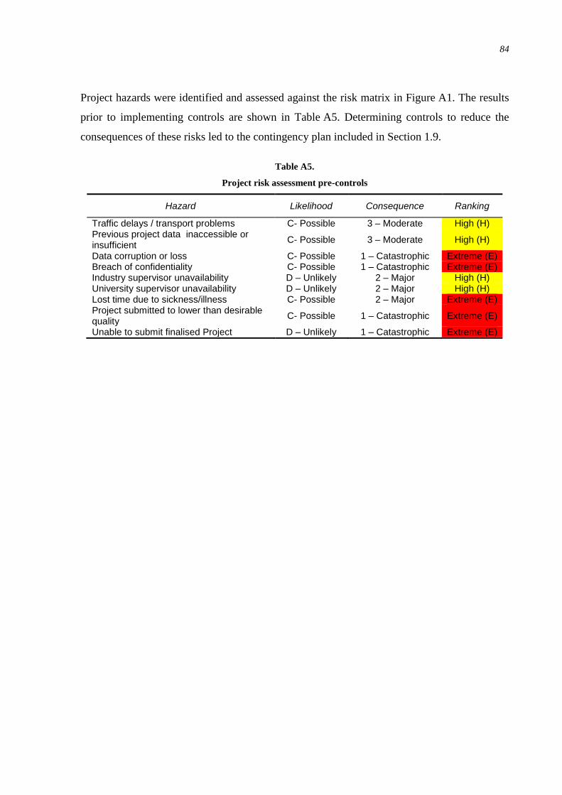
84
Project hazards were identified and assessed against the risk matrix in Figure A1. The results
prior to implementing controls are shown in Table A5. Determining controls to reduce the
consequences of these risks led to the contingency plan included in Section 1.9.
Table A5.
Project risk assessment pre-controls
Hazard Likelihood Consequence Ranking
Traffic delays / transport problems C- Possible 3 – Moderate High (H) Previous project data inaccessible or insufficient
C- Possible 3 – Moderate High (H)
Data corruption or loss C- Possible 1 – Catastrophic Extreme (E) Breach of confidentiality C- Possible 1 – Catastrophic Extreme (E) Industry supervisor unavailability D – Unlikely 2 – Major High (H) University supervisor unavailability D – Unlikely 2 – Major High (H) Lost time due to sickness/illness C- Possible 2 – Major Extreme (E) Project submitted to lower than desirable quality
C- Possible 1 – Catastrophic Extreme (E)
Unable to submit finalised Project D – Unlikely 1 – Catastrophic Extreme (E)

85
Figure A5. Project delivery schedule Page 1 of 2

86
Figure A5. Project delivery schedule Page 1 of 2

87
APPENDIX 2: EXISTING MINESCAPE PLOTS AND
XPAC SCHEDULE
In 2013, after an internal review of the project, a new mine plan was developed considering a
truck and shovel operation. As part of this mine plan, the geology, overburden thickness, coal
thickness and the new in-situ ratio were examined. These results are presented in the Figures A3
to A5 within this Appendix. A mine schedule was also created in XPAC at 5, 6 and 7 Mtpa
production target. The 5 Mtpa target schedule is shown in Figure A6.
Figure A3. Overburden thickness at the Wombat Project
(adapted from NHG, 2013).

88
Figure A4. In-situ coal thickness at the Wombat Project for seams UG to C
(adapted from NHG, 2013).
Figure A5. In-situ ratio plot at the Wombat Project - bcm in-situ waste/tonnes in-situ coal
(adapted from NHG, 2013).

89
Figure A6. 5 Mtpa creek diversion schedule
(adapted from NHG, 2013).

90
APPENDIX 3: GEOLOGY & GEOTECHNICAL DATA
Figure A7. Coal seam and ply representation for the Wombat Project
(Insite Geology, 2009).
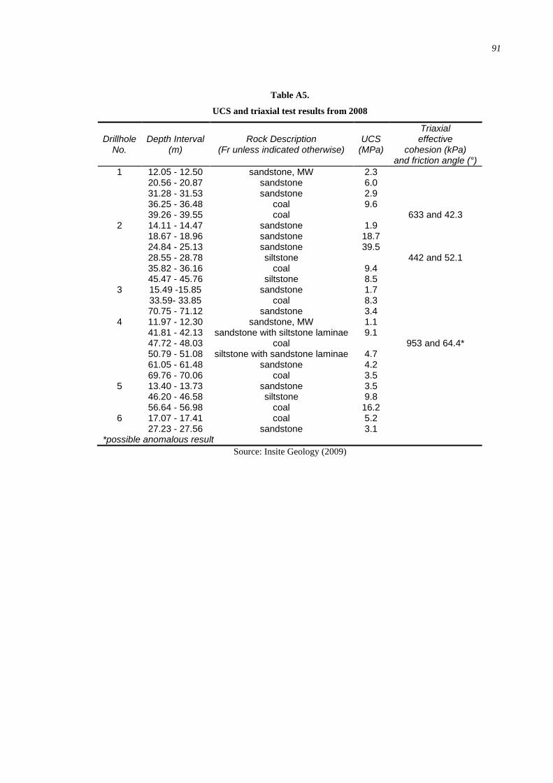
91
Table A5.
UCS and triaxial test results from 2008
Drillhole No.
Depth Interval (m)
Rock Description (Fr unless indicated otherwise)
UCS (MPa)
Triaxial effective
cohesion (kPa) and friction angle (°)
1 12.05 - 12.50 sandstone, MW 2.3 20.56 - 20.87 sandstone 6.0 31.28 - 31.53 sandstone 2.9 36.25 - 36.48 coal 9.6 39.26 - 39.55 coal 633 and 42.3
2 14.11 - 14.47 sandstone 1.9 18.67 - 18.96 sandstone 18.7 24.84 - 25.13 sandstone 39.5 28.55 - 28.78 siltstone 442 and 52.1 35.82 - 36.16 coal 9.4 45.47 - 45.76 siltstone 8.5
3 15.49 -15.85 sandstone 1.7 33.59- 33.85 coal 8.3 70.75 - 71.12 sandstone 3.4
4 11.97 - 12.30 sandstone, MW 1.1 41.81 - 42.13 sandstone with siltstone laminae 9.1 47.72 - 48.03 coal 953 and 64.4* 50.79 - 51.08 siltstone with sandstone laminae 4.7 61.05 - 61.48 sandstone 4.2 69.76 - 70.06 coal 3.5
5 13.40 - 13.73 sandstone 3.5 46.20 - 46.58 siltstone 9.8 56.64 - 56.98 coal 16.2
6 17.07 - 17.41 coal 5.2 27.23 - 27.56 sandstone 3.1
*possible anomalous result
Source: Insite Geology (2009)

92
Table A6.
UCS and triaxial test results from 2009
Drillhole No.
Depth Interval (m)
Rock Description (Fr unless indicated otherwise)
UCS (MPa)
Triaxial effective cohesion (kPa) and
friction angle (°)
1 16.39 - 16.79 mudstone 2.5 22.10 - 22.44 siltstone/sandstone 2.8
2 12.10 - 12.41 sandstone, fine grained, laminated
1.9
16.60 - 16.89 sandstone, coarse grained 1.6 18.67 - 18.99 coal 343 and 63 20.77 - 21.15 mudstone 4.4
3 11.85 - 12.10 carbonaceous mudstone 0.95 17.74 - 18.13 siltstone/sandstone 2.1 23.35 - 23.67 coal 833 and 67 26.06 - 26.48 siltstone 5.3
4 6.05 - 6.35 sandstone, coarse grained, MW
1.8
12.14 - 12.44 sandstone, coarse grained 4.3 16.96 - 17.25 sandstone, fine grained 8.5 24.16 - 24.37 siltstone, laminated 80 and 61 27.03 - 27.25 carbonaceous mudstone/coal 1.4 34.51 - 34.80 siltstone 8.7
5 12.05 - 12.37 siltstone 3.6 17.60 - 17.95 siltstone/sandstone 6.0 24.38 - 24.72 siltstone/sandstone 7.4 30.40 - 30.74 sandstone, coarse grained 9.2 33.74 - 34.06 sandstone, coarse grained 45.5 40.06 - 40.42 mudstone 277 and 58 51.74 - 52.02 sandstone 2.4 57.14 - 57.51 coal 1029 and 56
Source: Insite Geology (2010)
Table A7.
Peak and residual cohesion and shear angle for laminated rock types (2008)
Parameter 2008 results
Minimum Maximum Mean
Peak cohesion (kPa) 0 134 80 Peak shear angle (°) 14.6 24.6 20.3 Residual cohesion (kPa) 0 46 15 Residual shear angle (°) 9 26.4 18
Source: Insite Geology (2009)
Table A8.
Peak and residual cohesion and shear angle for laminated and non-laminated rock-types (2009)
Parameter Laminated rock types Non-laminated rock types
Minimum Maximum Mean Minimum Maximum Mean
Peak cohesion (kPa) 6 30 16.3 4 51 26.8 Peak shear angle (°) 14.8 18.6 16.4 15.1 17.9 16.5 Residual cohesion (kPa) 8 24 15.7 0 47 15.3 Residual shear angle (°) 13.2 18.5 15.7 15.1 17.2 16
Source: Insite Geology (2010)

93
Figure A8. East-west geological cross-section.
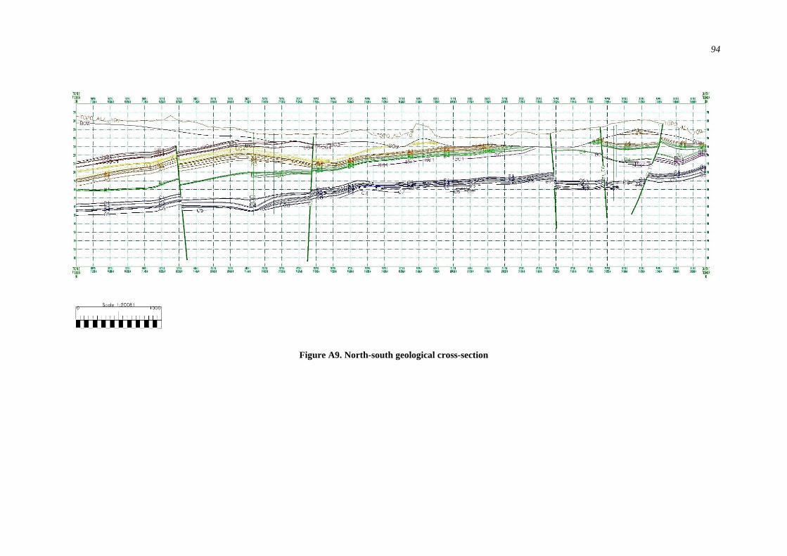
94
Figure A9. North-south geological cross-section
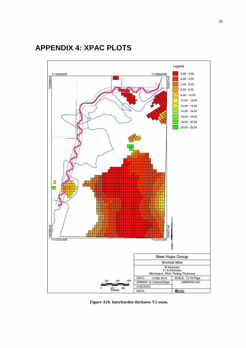
95
APPENDIX 4: XPAC PLOTS
Figure A10. Interburden thickness Y1 seam.
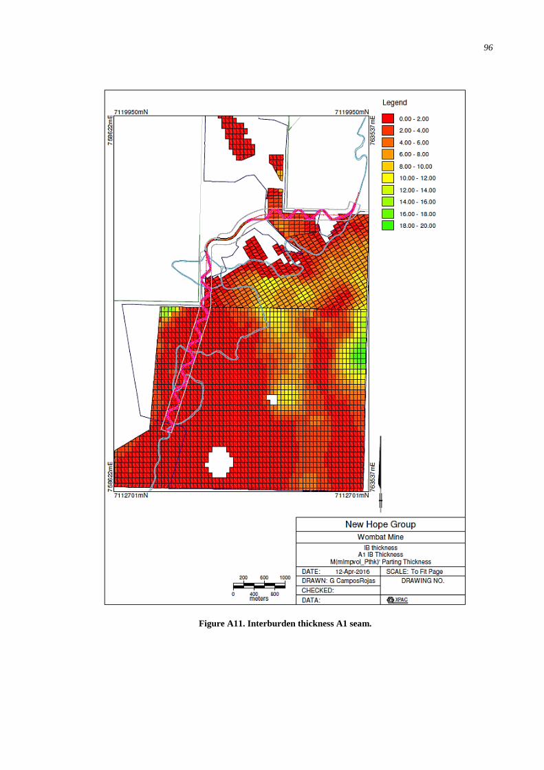
96
Figure A11. Interburden thickness A1 seam.

97
Figure A12. Interburden thickness B1 seam.

98
Figure A13. Interburden thickness C1 seam.
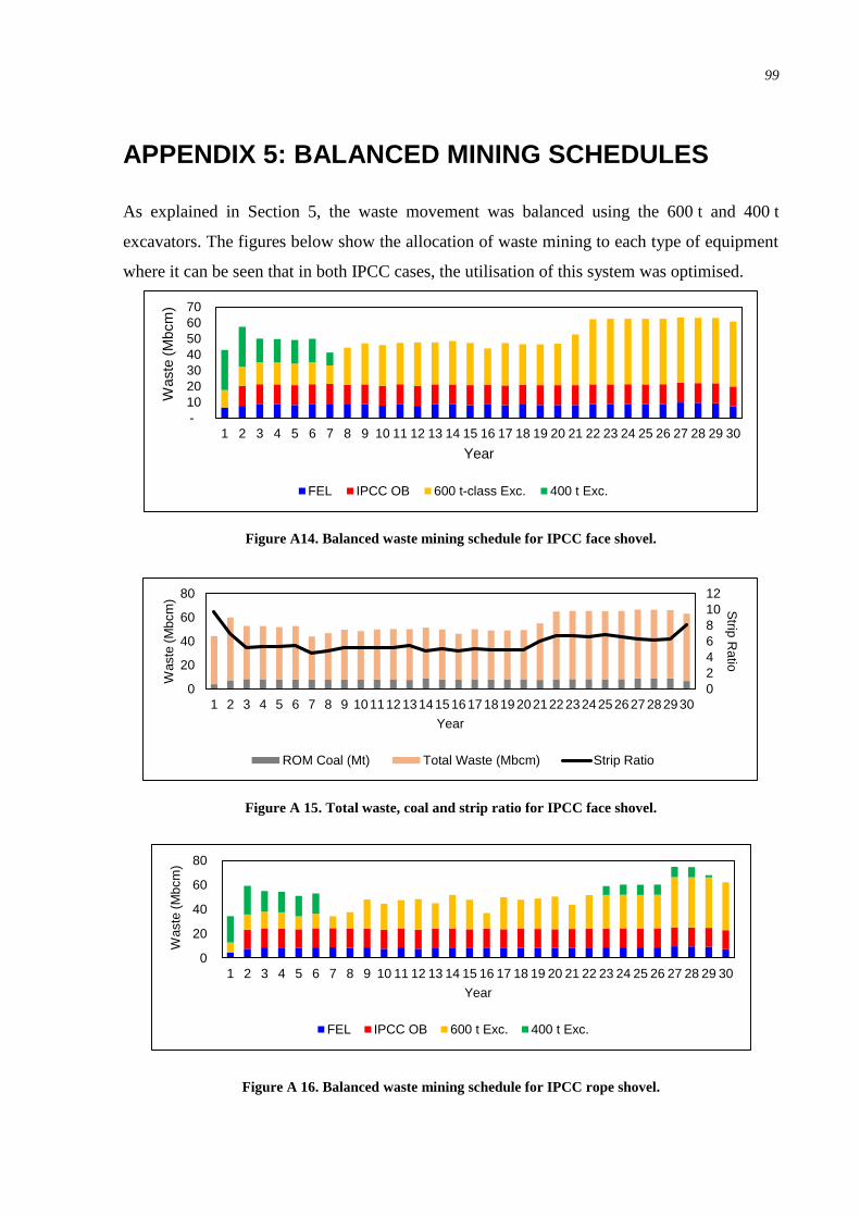
99
APPENDIX 5: BALANCED MINING SCHEDULES
As explained in Section 5, the waste movement was balanced using the 600 t and 400 t
excavators. The figures below show the allocation of waste mining to each type of equipment
where it can be seen that in both IPCC cases, the utilisation of this system was optimised.
Figure A14. Balanced waste mining schedule for IPCC face shovel.
Figure A 15. Total waste, coal and strip ratio for IPCC face shovel.
Figure A 16. Balanced waste mining schedule for IPCC rope shovel.
-
10
20
30
40
50
60
70
1 2 3 4 5 6 7 8 9 10 11 12 13 14 15 16 17 18 19 20 21 22 23 24 25 26 27 28 29 30
Waste
(M
bcm
)
Year
FEL IPCC OB 600 t-class Exc. 400 t Exc.
0
2
4
6
8
10
12
0
20
40
60
80
1 2 3 4 5 6 7 8 9 101112131415161718192021222324252627282930
Strip
Ratio
Waste
(M
bcm
)
Year
ROM Coal (Mt) Total Waste (Mbcm) Strip Ratio
0
20
40
60
80
1 2 3 4 5 6 7 8 9 10 11 12 13 14 15 16 17 18 19 20 21 22 23 24 25 26 27 28 29 30
Waste
(M
bcm
)
Year
FEL IPCC OB 600 t Exc. 400 t Exc.

100
Figure A 17. Total waste, coal and strip ratio for IPCC rope shovel.
Figure A 18. Balanced waste mining schedule for TEX.
Figure A 19. Total waste, coal and strip ratio for TEX.
0
2
4
6
8
10
0
20
40
60
80
1 2 3 4 5 6 7 8 9 101112131415161718192021222324252627282930
Strip
Ra
tio
Vo
lum
e (
Mb
cm
)
Year
ROM Coal (Mt) Total Waste (Mbcm) Strip Ratio
0
20
40
60
80
1 2 3 4 5 6 7 8 9 10 11 12 13 14 15 16 17 18 19 20 21 22 23 24 25 26 27 28 29 30
Waste
(M
bcm
)
Year
FEL IPCC OB 600 t Exc. 400 t Exc.
-
2
4
6
8
10
12
0
20
40
60
80
1 2 3 4 5 6 7 8 9 101112131415161718192021222324252627282930
Strip
Ratio
Waste
(M
bcm
)
Year
ROM Coal (Mt) Total Waste (Mbcm) ROM Strip Ratio

101
APPENDIX 6: TIME USAGE MODEL
A Time Usage Model (TUM) structure is shown in Figure A20 below.
Figure A20. Typical TUM structure
(Blunck, 2016).
In Figure A20, the following definitions apply (Blunck, 2016).
Calendar Time: Total hours in the period being examined. In this case the TUM was
based on a year; thus 8760 hours.
Mine Down: This is the time where no mining activities take place due to unplanned
circumstances such as bad weather or industrial action.
Planned Down: This is the time planned for equipment and process maintenance,
scheduled at least 24 hours in advance.
Unplanned Down: This is reactive maintenance downtime in which equipment does not
operate. It is an unplanned event.
Standby: Considers the time when the equipment is physically available and ready for
operation but it is not used due to disruptions caused by internal or external reasons.
These type of disruptions are normally longer than 20 minutes.
Operating delay: Caused by short duration disruptions (less than 10 minutes) caused by
operator’s events in which the equipment is being utilised but is not producing.
Productive Time: The time the equipment is in productive mining operation under the
control of an operator.
Ready Time: This is the total time available in the period under consideration that the
equipment is available for productive mining.

102
APPENDIX 7: PERSONNEL AND REHABILITATION
ASSUMPTIONS
Staff assumed for all models are detailed in Table A9.
Table A9.
Staff Assumptions
Staffing Requirements Total
General Manager 1
Business Support Officer 1
Safety
Safety Manager 1
Safety/Training Co-ordinator 1
Safety Assistants 2
Trainer & Assessors 1
Wash plant
CHPP Superintendents 1
Mining
Mining Manager 1
Superintendents 1
Pit OCE/Supervisor 5
Maintenance
Maintenance Manager 1
Maintenance Superintendents 1
Maintenance Planners 1
EEM 1
Maintenance Supervisors 4
Technical Services
Tech Services Manager 1
Senior Mining Engineer 2
Mining Engineers 2
Surveyors 2
Environmental 1
Geologist/Coal Quality 1
Drill and Blast Supervisor 1
Business
Human Resources 1
Reception 1
Purchasing 3
Source: NHG (2013)

103
For rehabilitation, the costs in Table A10 were assumed.
Table A10.
Rehabilitation Costs Assumptions
Disturbed Area Cost per Hectare (AUD/Ha)
Mining Area 9820 Pit Void 5860
Tailings Dam 70 000 Infrastructure 5860
Source: NHG (2013)

104
APPENDIX 8: EXCAVATOR AND TRUCK UNITS
Figure A21. Comparison of total loading units for LOM
Figure A22. Comparison of total hauling units for LOM
0
1
2
3
4
5
6
7
8
9
1 2 3 4 5 6 7 8 9 10 11 12 13 14 15 16 17 18 19 20 21 22 23 24 25 26 27 28 29 30
Units
Year
IPCC Face Shovel IPCC Rope Shovel TEX Revised Dragline
0
5
10
15
20
25
30
35
40
45
50
1 2 3 4 5 6 7 8 9 10 11 12 13 14 15 16 17 18 19 20 21 22 23 24 25 26 27 28 29 30
Units
Year
IPCC Face Shovel IPCC Rope Shovel TEX Revised Dragline