HAL Id: hal-00192527https://hal.archives-ouvertes.fr/hal-00192527

Submitted on 28 Nov 2007

HAL is a multi-disciplinary open accessarchive for the deposit and dissemination of sci-entific research documents, whether they are pub-lished or not. The documents may come fromteaching and research institutions in France orabroad, or from public or private research centers.

L’archive ouverte pluridisciplinaire HAL, estdestinée au dépôt et à la diffusion de documentsscientifiques de niveau recherche, publiés ou non,émanant des établissements d’enseignement et derecherche français ou étrangers, des laboratoirespublics ou privés.

Backlash fault detection in mechatronic system.R. Merzouki, Kamal Medjaher, M.A. Djeziri, B. Ould-Bouamama

To cite this version:R. Merzouki, Kamal Medjaher, M.A. Djeziri, B. Ould-Bouamama. Backlash faultdetection in mechatronic system.. Mechatronics, Elsevier, 2007, 17 (6), pp.299-310.10.1016/j.mechatronics.2007.03.001. hal-00192527

Backlash Fault Detection in MechatronicSystem

R. Merzoukia,1, K. Medjaherb, M. A. Djeziric

and B. Ould-Bouamamaa

aLAGIS UMR CNRS 8146, Ecole Polytechnique Universitaire de Lille, AvenuePaul Langevin, 59655 Villeneuve d’Ascq, France.

bLAB UMR CNRS 6596, Ecole Nationale Supérieure de Mécanique et desMicrotechniques, 26, Chemin de l’Epitaphe, 25030, Besançon, France.

cLAGIS UMR CNRS 8146, Ecole Centrale de Lille, Avenue Paul Langevin, 59655Villeneuve d’Ascq, France.

Abstract

In this paper, a fault detection and isolation model based method for backlashphenomenon is presented. The aim of this contribution is to be able to detect thendistinguish the undesirable backlash from the useful one inside an electromechanicaltest bench. The dynamic model of the real system is derived, using the bond graphapproach, motivated by the multi-energy domain of such mechatronic system. Theinnovation interest of the use of the bond graph tool, resides in the exploitation ofone language representation for modelling and monitoring the system with presenceof mechanical faults. Fault indicators are deduced from the analytical model andused to detect and isolate undesirable backlash fault, including the physical sys-tem. Simulation and experimental tests are done on electromechanical test benchwhich consists of a DC motor carrying a mechanical load, through a reducer partcontaining a backlash phenomenon.

Key words: Mechatronic system, Backlash, Fault Detection and Isolation,Residuals, Bond graph.

Introduction

For electromechanical systems, the growth of wear after a long operating pe-riod can engender a non neglected backlash. The undesirable presence of back-

1 Corresponding author: Tel. (+33) 328767486, Fax: (+33)320337189.E-mail address : Rochdi.Merzouki@polytech-lille.fr

Preprint submitted to Elsevier Science 14 March 2007

lash acts on the normal operation of the system and can cause considerabledamage for the equipment.

Backlash phenomenon is characterized by the existence of dead zone area,which describes the position gap between input and output system positions.Thus, an important dead zone affects the system performance during its con-trol in a closed loop.

In literature, many works have been realized around this topic, and can beclassified in three classes: those where the main interest is the control of suchsystems (e.g. [14], [13]), others are interesting in modelling and identification(e.g. [7], [8]), and for the third class, detection and evaluation of such phe-nomenon is developed (e.g. [3]). For this last class, two methods of diagnosisexists in the literature: with and without model. Methods without model arebased on a training under normal and failing operation (e.g. [9,15]), whichrequires the availability of a well developed fault database for the acquisitionof the failing modes. For backlash phenomenon, which describes a mechanicalimperfection intern to the system, it is difficult to introduce it from outside thesystem. Thus, a model based diagnosis method, based on comparison betweenthe nominal model output and the actual operation output is used in thiswork, where the diagnosis results are strongly dependent on the used model.

Usually, in mechatronic systems, several types of energy are involved. To modelthis kind of systems, one needs a unified tool like bond graph [10], to repre-sent the involved multiple energy domains. Furthermore, structural properties(observability, invertibility, monitorability, etc.) [2] of bond graph can help ingenerating fault indicators and fault detection algorithms.

Compared to structural analysis, the use of bond graph allows dealing with onetool from modelling to ARR generation. Whereas, using structural analysisto generate ARRs, one needs first the availability of the constraints list inorder to build the bipartite graph and to eliminate the unknown variablesby using the incidence matrix. Furthermore, with structural analysis method,the elimination of unknown variables from the constraints is not trivial forcomplex systems. However, by using bond graphs, it is well known that for anobservable system there are as many residuals as number of sensors presenton the physical system [4]. So, once the junction equations are written, theelimination procedure is straight forward by using the causal paths from theknown to unknown variables on the bond graph model, used in differentialcausality.

In this work, a contribution on how to detect and to locate the failures in-troduced by the mechanical backlash is proposed. The main purpose is todistinguish the disturbing backlash from the useful one during a normal op-eration of an electromechanical system. The useful backlash is defined by the

2

initial and non-perturbed dead zone area, necessary for the transient dynam-ics of the global system. When the dead zone excess its acceptable value, thebacklash phenomenon is created and the system will be perturbed.

This paper is organized as follows: after a short description of the electro-mechanical test bench, a global description of the system modelling is given inSection 3. In Section 4 details on the developed Fault Detection and Isolation(FDI) contribution are presented. Sections 5 and 6 are devoted to simulationand experimental results done on the electromechanical bench, respectively.Finally, a conclusion is given at the end of this paper.

1 Electromechanical actuator description

The test bench presented in Fig. 1 has been developed to identify some me-chanical imperfections such as: friction ,backlash and flexion. It was developedaccording to a specifications relating on continuous modeling of backlash, flex-ibility and friction torques [7]. It describes an electromechanical system madeup of a motor reducer involving an external load. The motor part is actu-ated by a DC motor delivering a relative important mass torque. This testbench contains mechanical imperfections such as: friction, backlash and elas-ticity within the transmission system. Its advantage is that one can vary theamplitudes of the mechanical imperfections located in the load part (Fig. 1).Coulomb friction is represented by a contact of various components of thesystem with different rigidities. Viscous friction depends on the viscosity ofthe lubricant contained between surfaces in contact. Backlash phenomenonis represented by two independent mechanical parts, whose transmission iscarried out via a dead zone varying between 0 and 24 degrees. A spring sys-tem is placed between the two mechanical parts in order to deliver a smoothtransmission.

On this test bench, one can measure the input and output positions of thereducer part by using two incremental encoders (Fig. 1).

2 Test bench global model

The electromechanical system of Fig. (1) can be considered as a concatena-tion of four parts: electrical part of DC motor, mechanical part of DC motor,reducer part and load part (Fig. 2). In the following modelling, the static fric-tion effects are not considered for mechanical aspect. Only a viscous friction,backlash phenomenon and flexibility of the transmission links are taken intoaccount as a mechanical imperfections.

3

Fig. 1. Electromechanical system.

sθ

eθ

LoadLoad partpart

DC DC MotorMotor

Reducer part

DC Motor

Mechanical part

Electrical part

Backlash

Elastic link

sθ

eθ

LoadLoad partpart

DC DC MotorMotor

Reducer part

DC Motor

Mechanical part

Electrical part

Backlash

Elastic link

Fig. 2. Electromechanical system parts.

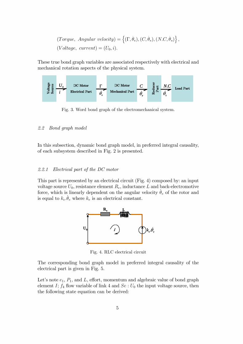
2.1 Word bond graph

The word bond graph represents the technological level of the model wherethe global system is decomposed into four subsystems (Fig. 3). Compared toclassical block diagram, in this representation, the input and output of eachsubsystem are defined by power variables represented by a conjugated pair ofeffort-flow (e, f). The power variables used for the studied system are:

4

(Torque, Angular velocity) =n(Γ,

.

θe), (C,.

θe), (N.C,.

θs)o,

(V oltage, current) = (U0, i).

These true bond graph variables are associated respectively with electrical andmechanical rotation aspects of the physical system.

DC Motor

Electrical Part

DC Motor

Mechanical PartLoad Part

Red

ucer

P

art

Vol

tage

So

urce 0U

ieθ

Γ

e

Cθ

.

s

N Cθ

DC Motor

Electrical Part

DC Motor

Mechanical PartLoad Part

Red

ucer

P

art

Red

ucer

P

art

Vol

tage

So

urce

Vol

tage

So

urce 0U

ieθ

Γ

e

Cθ

.

s

N Cθ

Fig. 3. Word bond graph of the electromechanical system.

2.2 Bond graph model

In this subsection, dynamic bond graph model, in preferred integral causality,of each subsystem described in Fig. 2 is presented.

2.2.1 Electrical part of the DC motor

This part is represented by an electrical circuit (Fig. 4) composed by: an inputvoltage source U0, resistance element Re, inductance L and back-electromotiveforce, which is linearly dependent on the angular velocity θe of the rotor andis equal to ke.θe where ke is an electrical constant.

Re L

U0 i .e ek θ

Re L

U0 i .e ek θ

Fig. 4. RLC electrical circuit

The corresponding bond graph model in preferred integral causality of theelectrical part is given in Fig. 5.

Let’s note e1, P1, and L, effort, momentum and algebraic value of bond graphelement I; f4 flow variable of link 4 and Se : U0 the input voltage source, thenthe following state equation can be derived:

5

Voltage

1Se:U0

R: Re

I: L

2

301

GY: ke

Mechanical P

art

DC Motor: Electrical Part

4Voltage

1Se:U0

R: Re

I: L

22

330011

GY: ke

GY: ke

Mechanical P

art

DC Motor: Electrical Part

44

Fig. 5. Bond graph model of electrical part.

e1 =dP1dt

= −Re.P1L− ke.f4 + U0, (1)

By replacing the effort and flow bond graph variables by their correspondingelectrical ones of Fig. 4, Eq. (1) can be written as:

L.di

dt= −Re.i− ke.

.

θe + U0. (2)

The gyrator (GY ) element on the bond graph model represents the powertransfer from electrical to mechanical part.

2.2.2 Mechanical part of the DC motor

This subsection describes the mechanical part of the DC motor representedby its inertia Je, viscous friction coefficient fe, transmission axis elasticity Kand a motorized torque U . In this part, the influence of backlash phenomenonis expressed by a disturbing torque w, and represented by a modulated effortsource in the bond graph model. The corresponding bond graph model of themechanical part is given by Fig. 6.

1

R: fe

0

Mse: w

eθ

U

C: K

DC Motor:

Mechanical Part

Red

ucer

Par

t

4

5 6

7

89

10

Ele

ctri

cal P

art

I: Je

1

R: fe

0

Mse: w

eθ

U

C: K

DC Motor:

Mechanical Part

Red

ucer

Par

t

44

55 66

77

8899

1010

Ele

ctri

cal P

art

I: Je

Fig. 6. Bond graph model of mechanical part.

In order to understand the role of the modulated effort source (Mse : ω), it isworth explaining the backlash mechanism inside the electromechanical system.

6

Backlash mechanism is constituted of two mechanical and unconnected bodies(Fig. 7), where ‘Body 1’ tries to transmit motion to ‘Body 2’ via a deadzone of amplitude 2.j0 (j0 is dead zone magnitude). The transmission will becorrect when the two bodies are in contact (i.e. bodies positions are identical).Otherwise (i.e. bodies are not contacted), the transmission will be delayed dueto the presence of a dead zone. The analytical relation between the bodiespositions is described by a hysteresis behavior relation. However, in order toavoid discontinuous disturbances due to a rigid contact, a smooth contact areahas been realized for the test bench. This is used to deaden the shock of thecontact and is modelled by a spring system of rigidity K (Fig. 7).

Body 1

positionvelocity

Body 2 Contact Elasticity

02 j j

Body 1

positionvelocity

Body 2 Contact Elasticity

02 j j

Fig. 7. Backlash mechanism.

Thus, a smooth and continuous model of transmitted torque w, which is de-veloped in [6] and illustrated in Fig. 8, is chosen to be identified and used asa modulated effort source (Mse : w). This latter includes a sigmoid functionexpressed by the following relation:

w = −4.K.j0.1− e−γ.z

1 + e−γ.z, (3)

where z is the difference between input and output reducer positions and γthe slope constant.

By adding the disturbing torque w, Eq. (3) to the linear transmitted torqueC0, which describes a flexible link given by:

C0 = K.z, (4)the approximate continuous transmitted torque C is obtained as follows:

C = K.

Ãz − 4.j0.

1− e−γ.z

1 + e−γ.z

!. (5)

Since the real backlash amplitude j0 is equal to a constant, its time variationis null. The disturbing torque w has a sigmoid function form, characterizedby its decreasing slope constant γ. The slope γ is chosen to give the bestapproximation of the transmitted torque inside the dead zone defined withinthe interval [−j0,+j0] of Fig. 8.

7

-4 -3 -2 -1 0 1 2 3 4-4

-3

-2

-1

0

1

2

3

4

Position (rad)

Torq

ue (N

.m)

disturbing torque w linear transmitted torque Cotransmitted torque via dead zone C

Fig. 8. Approximation of transmitted torques.

Let’s note e5, P5, Je, effort, momentum and algebraic value of element I, f4flow variable of link 4, f9,K flow and algebraic value of bond graph element C,and MSe : w the modulated effort source. Thus, the following state equationcan be derived:

e5 =dP5dt

= −R7.P5Je+ ke.f4 + w −K.

Zf9.dt. (6)

By replacing the bond graph variables by their corresponding mechanical andelectrical ones, Eq. (6) becomes:

Je...

θe = −fe..

θe + ke.i+ w −K.z. (7)

2.2.3 Reducer part

This part deals with the mechanical gears which link the mechanical and theload parts with a reduction constant N . Bond graph model of this physicalsubsystem is given by Fig. 9 where the reducer is represented by a transformerelement TF between the motor axis (with velocity θe) and the load (withvelocity θs).

TF

Reducer Part

: N

Mec

hani

cal

Par

t

Load

Par

t

10

11TF

Reducer Part

: N

Mec

hani

cal

Par

t

Load

Par

t

TF

Reducer Part

: N

Mec

hani

cal

Par

t

Load

Par

t

1010

1111

Fig. 9. Reducer part bond graph model.

8

The constitutive relation of the bond graph element TF , of Fig. 9, is writtenas:

f10 = N.f11, (8)

where f10 and f11 are the corresponding flow variables of links 10 and 11. Inmechanical domain, Eq. (8) becomes:

.

θe = N.θs. (9)

2.2.4 Load part

This part describes the load part of the electromechanical system. It is repre-sented by its inertia Js, viscous friction coefficient fs and backlash disturbingtorque N.w. Its corresponding bond graph model is given by Fig. 10.

1

Mse: Nw

sθ

R: fs

I: Js1112

13

14

Red

ucer

Par

t

1

Mse: Nw

sθ

R: fs

I: Js11111212

1313

1414

Red

ucer

Par

t

Fig. 10. Load part bond graph model.

Let’s note e14, P14, Js, effort, momentum and algebraic value of element I, f9,K flow and algebraic value of bond graph element C (Fig. 6); andMSe : N.wthe modulated effort source. The following relation can then be deduced fromthe 1 junction of Fig. (10):

e14 = −R12.P14Js+ Se13 +N.K.

Zf9.dt. (10)

After replacing the bond graph variables of Eq. (10) by their correspondingmechanical ones, one can get:

Js...

θs = −fs..

θs +N.w +N.K.z. (11)

2.2.5 Electromechanical global bond graph model

A concatenation of the bond graph models of the different parts describedabove leads to the global bond graph model of the electromechanical system

9

given in Fig. 11.

Voltage

1Se:U0

R: Re

DC Motor:

Electrical Part

GY

I: L

: ke

1

R: fe

0

Mse: w

eθ

U

C: KI: J

e

TF: N

1

Mse: Nw

sθ

R: fs

I: Js

DC Motor:

Mechanical Part

Red

ucer

P

art

Load Part

2

3 4

5 6

7

89

10 1112

13

1401Voltage

1Se:U0

R: Re

DC Motor:

Electrical Part

GY

I: L

: ke

1

R: fe

0

Mse: w

eθ

U

C: KI: J

e

TF: N

1

Mse: Nw

sθ

R: fs

I: Js

DC Motor:

Mechanical Part

Red

ucer

P

art

Load Part

22

33 44

55 66

77

8899

1010 11111212

1313

14140011

Fig. 11. Global bond graph model of the electromechanical system.

The dynamic and nonlinear model of the test bench, including the backlash,deduced from the global bond graph model is given by the following relations:

⎧⎪⎪⎪⎪⎪⎪⎪⎪⎨⎪⎪⎪⎪⎪⎪⎪⎪⎩

L.didt+Re.i+ ke.θe = U0,

Je.θe + fe.θe + w +K.z = Γ,

Js.θs + fs.θs = N.w +N.K.z,

z = θe −N.θs;

(12)

where Γ = ke.i, is the input motorized torque.

Fig. 12 represents the correspondence between the bond graph models and thephysical system parts. This is done to show the location of undesired backlashimperfection.

3 Simulation tests

3.1 Software Implementation

Simulation step is done on a specific bond graph software SYMBOLS 2000[12], which is an object oriented hierarchical modelling software. It allowsusers to create models using bond graph, block-diagram and equation models.Differential causalities and algebraic loops are solved out using its powerfulsymbolic solution engine. Nonlinearities and user code can be integrated in sin-gle editing IDE (Integrated Development Environment). The iconic modellingfacility allows system-morphic model layout. It also has many post-processingfacilities over the simulated result. Thanks to a developed generic item data-base which consists of a set of predefined models, and has been incorporated

10

sθ

eθ

LoadLoad

DC DC MotorMotor

Voltage

1Se:U0

R: Re DC Motor

Electrical Part

Motor axis

I: L

GY: ke

TF

Reducer Part

: N

Mec

hani

cal

Par

t

Load

Par

t

I: Js

Red

ucer

Par

t

Load Part

1

Mse: Nω

sθ

R: fs

Mse: ω C: K

1

R: fe

0

eθ

U

I: Je

DC Motor:

Mechanical Part

Reducer

part

Electrical

part

sθ

eθ

LoadLoad

DC DC MotorMotor

Voltage

1Se:U0

R: Re DC Motor

Electrical Part

Motor axis

I: L

GY: ke

Voltage

1Se:U0

R: Re DC Motor

Electrical Part

Motor axis

I: L

GY: ke

GY: ke

TF

Reducer Part

: N

Mec

hani

cal

Par

t

Load

Par

t

TF

Reducer Part

: N

Mec

hani

cal

Par

t

Load

Par

t

I: Js

Red

ucer

Par

t

Load Part

1

Mse: Nω

sθ

R: fs

I: Js

Red

ucer

Par

t

Load Part

1

Mse: Nω

sθ

R: fs

Mse: ω C: K

1

R: fe

0

eθ

U

I: Je

DC Motor:

Mechanical Part

Reducer

part

Electrical

part

Mse: ω C: K

1

R: fe

0

eθ

U

I: Je

DC Motor:

Mechanical Part

Reducer

part

Electrical

part

Fig. 12. Correspondence bond graph - electromechanical system.

as capsules in the software SYMBOLS 2000, the designer can easily build thedynamic models of several physical systems from the Process and Instrumen-tation Diagram (P&ID) by just connecting different sub models. The globaldynamic in symbolic format is obtained connecting different icons. Behindeach submodel the bond graph model is hinted (Fig. 13). If parameter val-ues are available, the model can be simulated using own Symbols function orMatlab, S − Function

3.2 Simulation results

Simulation parameters used for the electromechanical system are given in table(1).

For an input voltage signal like that one of Fig. 14, one can obtain the graph-ical characteristic of the backlash disturbing torque of Fig. 15 and the globaltransmitted torque to the load of Fig. 16. This latter shows a dead zone ofmagnitude 2.j0 = 0, 4 rad and a linear transmitted torque outside the deadzone.

11

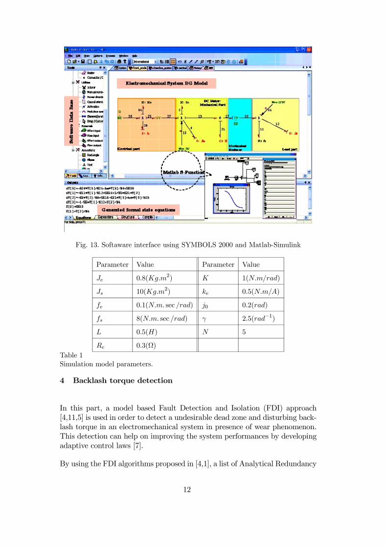
Fig. 13. Softaware interface using SYMBOLS 2000 and Matlab-Simulink

Parameter Value Parameter Value

Je 0.8(Kg.m2) K 1(N.m/rad)

Js 10(Kg.m2) ke 0.5(N.m/A)

fe 0.1(N.m. sec /rad) j0 0.2(rad)

fs 8(N.m. sec /rad) γ 2.5(rad−1)

L 0.5(H) N 5

Re 0.3(Ω)

Table 1Simulation model parameters.

4 Backlash torque detection

In this part, a model based Fault Detection and Isolation (FDI) approach[4,11,5] is used in order to detect a undesirable dead zone and disturbing back-lash torque in an electromechanical system in presence of wear phenomenon.This detection can help on improving the system performances by developingadaptive control laws [7].

By using the FDI algorithms proposed in [4,1], a list of Analytical Redundancy

12

0 1 2 3 4 5 6 7 8 9 10-2

-1.5

-1

-0.5

0

0.5

1

1.5

2

Time (s)

Inpu

t Vol

tage

(V)

Fig. 14. Input voltage.

-1.5 -1 -0.5 0 0.5 1 1.5 2-0.8

-0.6

-0.4

-0.2

0

0.2

0.4

0.6

0.8

Position (rad)

Dis

turb

ing

Torq

ue (N

.m)

Fig. 15. Backlash disturbing torque.

-1.5 -1 -0.5 0 0.5 1 1.5 2-0.6

-0.4

-0.2

0

0.2

0.4

0.6

0.8

1

1.2

Tran

smitt

ed T

orqu

e (N

.m)

Position (rad)

Fig. 16. Transmitted torque via a dead zone and flexible link.

Relation (ARR) along with the corresponding Fault Signature Matrix (FSM)can be generated. These tools allow to detect and isolate the possible faultspresent on the physical system. Note that for this application, and comparingwith the existing model based FDI methods where the faults are not modelled;in the proposed contribution the backlash is considered as a fault and takeninto account in the system dynamic model. So, its related variables appearin the generated ARR and its dynamics can be simulated through the ARRequations by using an appropriate software.

13

The main steps to generate the list of ARR and the FSM by using the methoddeveloped in [4] are summarized bellow:

• Build the bond graph model in preferred integral causality.• Put the bond graph model in preferred derivative causality (with sensorcausality inversion if necessary).

• Write the constitutive relation for each junction.• Eliminate the unknown variables from each constitutive relation by coveringthe causal paths on the bond graph model.

• Generate the list of ARR and the corresponding FSM.

Note that for an observable system, with none unresolved algebraic loops, thenumber of ARR generated is equal to the number of detectors on the bondgraph model [4].

The bond graph model, in derivative causality, of the system under study isshown in Fig. 17.

11

Se:U0

R: Re

DC Motor:

Electrical Part

GY

I: L

: ke

12

R: fe

01

Mse: w

U

C: KI: J

e

TF: N

13

Mse: Nw

R: fs

I: Js

DC Motor:

Mechanical Part

Red

ucer

P

art

Load Part

2

3 4

5 6

7

89

10 1112

13

1401

sθDf: eθDf:

1615

11

Se:U0

R: Re

DC Motor:

Electrical Part

GY

I: L

: ke

12

R: fe

01

Mse: w

U

C: KI: J

e

TF: N

13

Mse: Nw

R: fs

I: Js

DC Motor:

Mechanical Part

Red

ucer

P

art

Load Part

22

33 44

55 66

77

8899

1010 11111212

1313

14140011

sθDf: sθDf: eθDf: eθDf:

16161515

Fig. 17. Bond graph model in derivative causality of the system.

The constitutive relations of junctions ‘11’, ‘12’, ‘01’ and ‘13’ are given by thefollowing equations:

e2= e0 − e1 − e3, (13)e15= e4 − e5 + e6 − e7 − e8, (14)f10= f8 − f9, (15)e11= e12 + e14 + e16 − e13. (16)

Two structurally independent ARR can be generated from Eqs. (14) and (15)after eliminating the unknown variables. This is because the system is struc-turally observable and does not contain any algebraic loop. The unknownvariables elimination process is achieved by following the causal paths, fromknown to unknown variables, on the bond graph model.

For Eq. (14) the unknown variables e15, e5, e6, e7 and e8 can be calculated asfollows:

14

⎧⎪⎪⎪⎪⎪⎪⎪⎪⎪⎪⎪⎪⎪⎪⎨⎪⎪⎪⎪⎪⎪⎪⎪⎪⎪⎪⎪⎪⎪⎩

e15 = 0,

e5 = Je.df5dt= Je.

dθedt

,

e6 = w,

e7 = fe.f7 = fe.θe,

e8 = e10 =1N.e11 =

1N.

Ãfs.θs −N.w + Js.

dθsdt

!.

(17)

Once the variable e4 is determined, Eq. (14) can be written only in terms ofknown variables which is in fact an ARR. Eq. (13) can be rewritten as:

e3 = U0 − e2 − e1 = U0 −Re.f3 − L.df3dt

, (18)

with

⎧⎪⎪⎪⎪⎪⎪⎨⎪⎪⎪⎪⎪⎪⎩

f3 =1ke.e4,

e4 = Je.dθedt− w + fe.θe +

1N.

Ãfs.θs −N.w + Js.

dθsdt

!,

e3 = ke.f4 = ke.θe.

(19)

Then Eq. (18) becomes

ke.θe = U0 −Re

ke.e4 −

L

ke.de4dt

. (20)

The following first ARR is then deduced by replacing the expression of e4,calculated from Eq. (19), in Eq. (20):

ARR1 : ke.θe − U0 +Re

ke.

ÃJe.

dθedt− w + fe.θe +

1N

Ãfs.θs −N.w + Js.

dθsdt

!!

+ Lke. ddt

ÃJe.

dθedt− w + fe.θe +

1N

Ãfs.θs −N.w + Js.

dθsdt

!!= 0.

The second ARR can be deduced from equation 15. The unknown variablesf10, f8 and f9 of this equation can be calculated from the known ones asfollows:

15

⎧⎪⎪⎪⎪⎪⎨⎪⎪⎪⎪⎪⎩f10 = N.f11 = N.θs,

f8 = f15 = θe,

f9 =1K.de9dt= 1

K.N. d

dt(e12 + e14 + e16 − e13) ;

(21)

where

⎧⎪⎪⎪⎪⎪⎪⎪⎪⎪⎨⎪⎪⎪⎪⎪⎪⎪⎪⎪⎩

e13 = N.w,

e12 = fs.f12 = fs.θs,

e14 = Js.df14dt

= Js.dθsdt

,

e16 = 0.

(22)

The second ARR is then deduced by replacing the unknown variables of Eqs.(21) and (22) in Eq. (15):

ARR2 : N.d

dt

Ãfs.θs + Js.

dθsdt−N.w

!+K.

³N.θs − θe

´= 0.

Once the list of ARR is generated, the FSM can be built by deducing thesignatures of the system components on each residual. Note that each com-ponent in the physical system can be represented by one or more variable(or parameters) in the residuals. A residual ri is a numerical evaluation of anARRi. The corresponding residuals r1 and r2 of ARR1 and ARR2 are givenby the following relations:

r1 = ke.θe − U0 +Re

ke.

ÃJe.

dθedt− w + fe.θe +

1N

Ãfs.θs −N.w + Js.

dθsdt

!!

+ Lke. ddt

ÃJe.

dθedt− w + fe.θe +

1N

Ãfs.θs −N.w + Js.

dθsdt

!!,

r2 = N. ddt

Ãfs.θs + Js.

dθsdt−N.w

!+K.

³N.θs − θe

´.

The corresponding FSM of the system under study is given in table 2.

In this table 2, the rows represent the components signatures and the columnsare respectively fault detectability Db, fault isolability Ib, and first and secondresidual r1 and r2. A ‘1’ value on respectively Db and Ib columns means that

16

Db Ib r1 r2

Input velocity sensor θe 1 0 1 1

Output velocity sensor θs 1 0 1 1

Electrical partL

R

1

1

0

0

1

1

0

0

Mechanical partJe

fe

1

1

0

0

1

1

0

0

Disturbing torque w 1 0 1 1

Load partJs

fs

1

1

0

0

1

1

1

1

Table 2Fault signature matrix of the electromechanical system.

faults on the corresponding components are detectable and isolable. The pres-ence of ‘1’ value on r1 and r2 columns shows the influence of the correspondingcomponents on the residual dynamics.

In this application, the FSM helps to detect the presence of backlash phenom-enon issued from a possible mechanical wear.

5 Simulation Results

Simulation tests have been done on backlash system model of Fig. 1, whereinertia, friction and dead zone parameters have been identified in [6] and givenin table 1. These simulation tests allow to show how backlash phenomenoncan be detected for typical electromechanical system of Fig. 1, by using theFDI algorithm described before. The software tool used for this simulationis SYMBOLS 2000 to generate the ARRs and their corresponding residualsin symbolic form, then Matlab − Simulink for numerical results. Tests havebeen done with an open loop scheme, where only input and output positionsof reducer part are experimentally measured. Note that for the studied testbench system, the dead zone magnitude could be varied until 0, 2 rad. So, ifthis magnitude is maintained with the elasticity characteristic given in table1, the estimated disturbing torque w will describe the sigmoid curve of Fig.18 and expressed in Eq. (3).

As shown in Fig. 19(c) and Fig. 19(d), while the input reducer axis rotates ataround 5, 2 rad/s, the input one goes to 1, 7 rad/s; where each axis followssuccessively trajectories of Fig. 19(a) and Fig. 19(b). For this slow motion,

17

-0.8 -0.6 -0.4 -0.2 0 0.2 0.4 0.6 0.8-5

-4

-3

-2

-1

0

1

2

3

4

5

Input-Output positions difference (rad)

Dis

turb

ing

torq

ue (N

.m)

Fig. 18. Disturbing torque evolution.

one needs to detect the fault issued from backlash phenomenon in order toillustrate its impact on nominal system operating. In this case, mechanicaltransmission inside the reducer part of the system given in Fig. (1) is rep-resented by a flexible link and a dead zone area varying between 0 and 0, 2rad.

Two distinct detections of dead zone are presented: the first one during tem-poral interval [7, 5; 12] s, where the disturbing torque w of Fig. 20(b) becomesnon null and varies from 0 to −4, 75 N.m. The disturbing torque w is in lineardependence of j0 (see Eq. (3)), so its variation out of zero value, shows thepresence of dead zone. This latter varies within [0; 0, 18] rad (Fig. 20(a)) andis noticed via evolution of ARR1 and ARR2 (Fig. 20(c) and Fig. 20(d)). Thesecond detection is given between [17; 21] s, where input and output positionsand velocities of reducer part given in Fig. 19(a), Fig. 19(b), Fig. 19(c) andFig. 19(d) are affected. This second detection presented in ARR1 and ARR2(Fig. 20(c) and Fig. 20(d)), by a positive residual values, shows an increase ofdisturbing torque (Fig. 20(b)) until zero value corresponding to position gap(Fig. 20(a)) due to flexible link of 1 rad.

18

Fig. 19. (a) Input reducer part position, (b) output reducer part position, (c) Inputreducer part velocity and (d) output reducer part velocity.

0 5 10 15 20 250

0.2

0.4

0.6

0.8

1

1.2

1.4

Time (s)(a)

Inpu

t-out

put p

ositi

ons

diffe

renc

e (ra

d)

0 5 10 15 20 25-5

-4.5

-4

-3.5

-3

-2.5

-2

-1.5

-1

-0.5

0

Time (s)(b)

Dis

turb

ing

torq

ue (N

.m)

Fig. 20. (a) Temporal evolution of input-output reducer position gap with presenceof dead zone, (b) temporal evolution of disturbing torque with dead zone variation,(c) dead zone variation acting on first ARR and (d) dead zone variation acting onsecond ARR.

19

Parameters N. Values Parameters N. Values

Jm 0.01(Kg.m2) N 1

fm 0.015(N.m. sec /rad) j0 0.1− 0.8(rad)

Js 0.00002(Kg.m2) L 1.9(H)

fs 0.02(N.m. sec /rad) Re 7.6(Ω)

Table 3System parameters.

6 Experimental Results

Experimental results have been done on system of (Fig. 1), where the systemparameters are given in table 3. These parameters are identified off-line onthe real system, using structural and analytical identification methods. A PDcontroller is applied on the real system with the coefficients KP = 1.25 andKD = 0.5.

At the fist step, the dead zone between the two independent mechanisms ofthe load part are mechanically eliminated (see Fig. 1). Then, control signal ofFig. (21-a) is applied, where input and output position signals are superposedin Fig. (21-b). The difference between the two positions is given by Fig. (21-c).Normally, the dead zone is eliminated mechanically, but it is already presentas it is shown in Fig. (21-d). This is due to the presence of initial dead zonewhich is not considered in the modelling and practically is located betweentransmitted gears and useful for the initial transmission. This initial dead zoneis taken as the tolerant value that we admit for the backlash phenomenon. Theresidual signals r1 and r2 in presence of this initial values are given successivelyFig. (21-e) and Fig. (21-f).

At the second step, we omitted the screw which link the two mechanisms of theload part (see Fig. 1). Then, an important dead zone area is introduced. For thesame control signal as presented in step one, it is applied again for the secondstep (see Fig. (22-a)), where the backlash effect is considerable according tothe position signals and their difference in Fig. (21-b) and Fig. (21-c). Thehysteresis characteristic between the positions, issued from the presence ofan important dead zone is illustrated in Fig. (21-d). Finally, residual signals,which show the increase of their amplitude comparing to the step1 are givenin Fig. (21-e) and Fig. (21-f). The asymmetric allure of the signals is due tothe initial position of the two mechanisms which is not confounds with themiddle of the dead zone.

20

0 5 10 15 20-0.15

-0.1

-0.05

0

0.05

Time (sec)

Diffe

renc

e Po

sitio

ns (r

ad)

0 5 10 15 20-1

-0.5

0

0.5

1

Time (sec)

Inpu

t-Out

put P

ositi

ons

(rad)

-b-

0 5 10 15 20-0.01

-0.005

0

0.005

0.01

Time (sec)-c-

Con

trol S

igna

l (N.

m)

-a--a--a-

-1 -0.5 0 0.5 1-1

-0.5

0

0.5

1

Input Position (rad)

Out

put P

ositi

on (r

ad)

-d-

0 5 10 15 20-0.02

-0.01

0

0.01

0.02

Time (sec)

r1

-e-

0 5 10 15 20-10

-5

0

5x 10-3

Time (sec)

r2

-f-

Input positionOutput Position

Fig. 21. Experiments with initial and significant backlash phenomenon: (a) InputControl Signal, (b) Input-Output Reducer Part, (c) Input-Output Difference Po-sition, (d) Input-Output Hysteresis Behavior, (e) Residual Signal 1, (f) ResidualSignal 2.

7 Conclusion

In this work, a model based FDI application on electromechanical system ispresented using bond graph approach. At first, the bond graph, in preferredintegral causality, is used to model the nonlinear electromechanical system,by combining the multi-physics dynamics. Then, this bond graph tool is usedto generate the residuals via the analytical redundancy relations, in order todetect the presence of perturbed backlash phenomenon. Finally, the fault sig-nature matrix is obtained from the residuals expressions, by putting the bondgraph model of the system in preferred derivative causality. These fault indica-tors allowed to monitor the physical system, and to distinguish the undesirablebacklash from the useful one by observing the residual responses as shown bythe simulation and the experimental results.

21

0 5 10 15 20-0.01

-0.005

0

0.005

0.01

Time (sec)

Cont

rol S

igna

l (N

.m)

-a-

0 5 10 15 20-1

-0.5

0

0.5

1

Time (sec)

Inpu

t-Out

put P

ositi

ons

(rad)

-b-

0 5 10 15 20-0.5

0

0.5

1

Time (sec)

Diffe

renc

e Po

sitio

ns (r

ad)

-c-

-1 -0.5 0 0.5 1-1

-0.5

0

0.5

Input Position (rad)

Out

put P

ositi

on (r

ad)

-d-

0 5 10 15 20-0.1

-0.05

0

0.05

0.1

Time (sec)

r1

-e-

0 5 10 15 20-0.02

0

0.02

0.04

0.06

Time (sec)

r2

-f-

Input PositionOutput Position

Fig. 22. Experiments with important backlash fault: (a) Input Control Signal, (b) In-put-Output Reducer Part, (c) Input-Output Difference Position, (d) Input-OutputHysteresis Behavior, (e) Residual Signal 1, (f) Residual Signal 2.

22

References

[1] B. Ould Bouamama, A.K. Samantaray, M. Staroswiecki, and G. Dauphin-Tanguy. Derivation of constraint relations from bond graph models for faultdetection and isolation. In International Conference on Bond Graph Modelingand Simulation (ICBGM’03), pages 104–109. Simulation Series Vol.35, No.2,ISBN 1-56555-257-1, 2003.

[2] G. Dauphin-Tanguy, A. Rahmani, and C. Sueur. Bond graph aided design ofcontrolled systems. Simulation Practice and Theory, 7(5-6):493–513, 1999.

[3] M. A. Djeziri, R. Merzouki, B. Ould Bouamama, G. Dauphin Tanguy. Faultdetection of backlash phenomenon in mechatronic system with parameteruncertainties using bond graph approach. In International Conference onMechatronics and Automation (ICMA’06), pages 600–605, Luoyang, China,June 25 - 28 2006.

[4] B. Ould Bouamama, K. Medjaher, A. K. Samantaray, and M. Staroswiecki.Supervision of an industrial steam generator. part I: Bond graphmodelling. Control Engineering Practice, 2005. In press, available online atwww.sciencedirect.com.

[5] R. Isermann. Supervision, fault detection and fault diagnosis methods - anintroduction. Control Engineering Practice, Vol. 5, No. 5:639–652, 1997.

[6] R. Merzouki, J. C. Cadiou, and N. K. M’Sirdi. Compensation of friction andbacklash effects in an electrical actuator. Journal of Systems and ControlEngineering, 218(12):75–84, March 2004.

[7] R. Merzouki and J. C. Cadiou. Estimation of backlash phenomenon inthe electromechanical actuator. Control Engineering Practice, 13(8):973–983,August 2005.

[8] R. Merzouki, J. A. Davila Montoya, L. M. Fridman and J. C. Cadiou.Backlash phenomenon observation and identification in electromechanicalsystem. Control Engineering Practice, Vol 15/4, pp 447-457, 2007.

[9] T. Murakami and N. Nakajima. Compter-aided design-diagnosis using featuredescription. In J.S. Gero, editor, Artificial Intelligence in Engineering: Diagnosisand Learning, pages 199–226. Elsevier, 1988.

[10] H.M. Paynter. Analysis and design of Engineering Systems. M.I.T. Press, 1961.

[11] M. Staroswiecki and G. Comtet-Varga. Analytical redundancy relations for faultdetection and isolation in algebraic dynamic systems. Automatica, 37:687–699,2001.

[12] A. Mukherjee and A.K. Samantaray. System modelling through bond graphobjects on SYMBOLS 2000. In International Conference on Bond GraphModeling and Simulation (ICBGM’01), pages 164–170. Simulation Series, Vol.33, No. 1, ISBN 1-56555-103-6, 2001.

23

[13] J. A. Tenreiro Machado. Variable structure control of manipulators withjoints having flexibility and backlash. Journal Systems Analysis-Modelling-Simulation, 23(0):93–101, 1996.

[14] G. Tao and P.V. Kokotovic. Contiuous-time adaptive control of systems withunknown backlash. IEEE Transactions on Automatic Control, 40(2):1083–1087, 1995.

[15] V. Venkatasubramanian, R. Rengaswamy, and S.N. Kavuri. A review of processfault detection and diagnosis. Part II: Qualitative models and search strategies.Computers and Chemical Engineering, 27:313–326, 2003.

24