backpropagation neural network based face detection in...

1email: [email protected]

Backpropagation neural network based face detection in frontal faces images

David Suárez Perera1

Neural & Adaptative Computation + Computational Neuroscience Research Lab Dept. of Computer Science & Systems, Institute for Cybernetics

University of Las Palmas de Gran Canaria

Las Palmas de Gran Canaria, 35307 Spain

University of Applied Sciences Brandenburg an der Havel, 14770

Germany

Abstract Computer vision is a computer science field belonging to artificial intelligence. The purpose of this branch is allowing computers to understand the physical world by visual media means. This document proposes an artificial neural network based face detection system. It detects frontal faces in RGB images and is relatively light invariant. Problem description and definition are enounced in the first sections; then the neural network training process is discussed and the whole process is proposed; finally, practical results and conclusions are discussed. Process has three stages: 1) Image preprocessing, 2) Neural network classifying, 3) Face number reduction. Skin color detection and Principal Component Analysis are used in preprocessing stage; back propagation neural network is used for classifying and a simple clustering algorithm is used on the reduction stage.

1 Introduction .......................................................................................................................................1

2 Problem Definition ............................................................................................................................1

3 Problem analysis ................................................................................................................................2

4 Process overview................................................................................................................................3 4.1 Image Preprocessing ..................................................................................................................4 4.2 Neural Network classifying.........................................................................................................4 4.3 Face number reduction ...............................................................................................................4

5 Classifier Training.............................................................................................................................5 5.1 Filtering ......................................................................................................................................6 5.2 Principal Component Analysis....................................................................................................7 5.3 Artificial Neural Network............................................................................................................8

5.3.1 Grayscale values .....................................................................................................................8 5.3.2 Horizontal and vertical derivates ............................................................................................9 5.3.3 Laplacian ..............................................................................................................................11 5.3.4 Laplacian and horizontal and vertical derivates values ........................................................12 5.3.5 Grayscale and Horizontal and vertical derivates values .......................................................13 5.3.6 Final comments ....................................................................................................................14

6 Results...............................................................................................................................................14 6.1 Test 1: Faces from the training dataset ....................................................................................15 6.2 Test 2: Hidden and scaled faces ...............................................................................................16 6.3 Test 3: Slightly rotated faces.....................................................................................................18

7 Conclusions ......................................................................................................................................19

8 References ........................................................................................................................................19

David Suarez 1 21/09/2005

1 Introduction This document proposed a method to detect faces in images following a neural network approach. Framed in the artificial intelligence field and more specifically in computer vision, face detection is a comparatively new problem in computer science. Until some years ago, computers were not able to do real time images processing; it is an important requirement for face detection applications. Face detection has several applications. It can be used for many task like tracking persons using an automatic camera for security purposes; classifying image databases automaticly or improving human-machine interfaces. In the artificial intelligence subject, accurate face detection is a step towards in the generic object identification problem [3]. First, the problem definition is enounced and in section 2 the problem definition is given. Section 3 analyzes problems and approaches. Section 5 overviews the whole process and describes skin detction and clustering algorithm. Section 4 is where the face classifier and its training method is proposed; it is the main part of the face detection process. Section 6 shows the process results and finally, the conclusions are enounced in section 7.

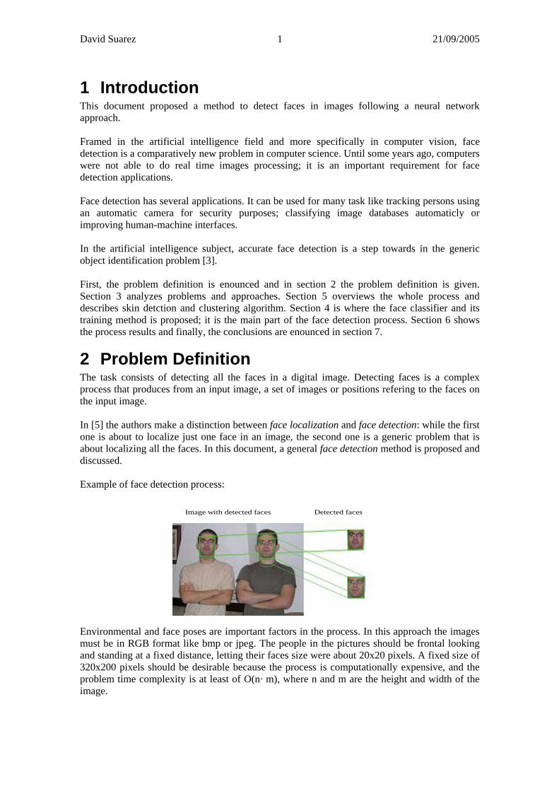
2 Problem Definition The task consists of detecting all the faces in a digital image. Detecting faces is a complex process that produces from an input image, a set of images or positions refering to the faces on the input image. In [5] the authors make a distinction between face localization and face detection: while the first one is about to localize just one face in an image, the second one is a generic problem that is about localizing all the faces. In this document, a general face detection method is proposed and discussed. Example of face detection process:

Environmental and face poses are important factors in the process. In this approach the images must be in RGB format like bmp or jpeg. The people in the pictures should be frontal looking and standing at a fixed distance, letting their faces size were about 20x20 pixels. A fixed size of 320x200 pixels should be desirable because the process is computationally expensive, and the problem time complexity is at least of O(n· m), where n and m are the height and width of the image.

Image with detected faces Detected faces


3 Problem analysis Face detection was not possible until 10 years ago because of the existing technology. Nowadays, there are several algorithmical techniques allowing face processing, but under several restrictions. Defining these restrictions in a given environment is mandatory before starting the application development. Face detection problem consists of detecting presence or absence of face-like regions in a static image (ideally, regardless its size, position, expression, orientation and light condition) and their localizations. This definition agrees the ones in [4] [5]. Allowing image processing and face detection in a finite and short amount of time requires the image fulfills next conditions: 1. Fixed size images: The images have to be fixed in size. This requirement can be achieved by

image preprocessing, but not always. If the input image has lower size than required, the magnification is inaccurate.

2. Constant ratio faces: The faces must be natural faces, around the correct proportions of an average face.

3. Pose: There are face localization techniques to find a rotated face in an image, it is achieved by harvesting face rotation invariant features. However, the neural network approach adopted in this document uses only simple features. This implies limited in-plane rotation (the faces must be looking at the direction normal to the picture at most)

4. Distance: The faces must be at such a distance that its size allows detection. It means about 20x20 pixels faces.

The output of face detection process is a set of normalized faces. The format of the normalized faces could be face images, positions of the faces in the original images, an ARFF dataset [2] or some other custom format. References [3] [5] describe the main problems in face detection. They are related with the following factors: 1. Face position: Face localization is affected by rotation (in-plane and out-of-plane) and

distance (scaled faces). 2. Face expression: There are facial expressions that modify the face form affecting the

localization process. 3. Structural components: Moustaches, barb, glasses, hairstyle and other complements difficult

the process. 4. Environment conditions: Light conditions, fog and other environmental factors affect

dramatically the process if it is mostly based on skin color detection. 5. Occultation: Faces hidden by objects or partially out of the image represent a handicap in the

process. There are four approaches for the face detection problem [5]: 1. Knowledge-based methods: It uses rules based on human knowledge of what is a typical

face to capture relations between facial features. 2. Feature invariant approaches: It uses structural invariants features of the faces. 3. Template matching methods: It uses a database of templates selected by experts of typical

face features (nose, eyes, mouth) and compare them with parts of the image to find a face. 4. Appearance-based methods: It uses some selector algorithm trained to learn face templates

from a data training set. Some of the trained classifiers are: neural network, bayes rule or k-nearest neighbor based.


The first and second approaches are used to face localization. Third works in localization and detection. And fourth is used mainly in detection. The method proposed in this study belongs to the appearance-based class. Authors achieved good results using neural network face localization in [6] [15], were they used a hierarchized neural network system with a high success: authors get some rotation and scale invariance by sub sampling and rotating image regions and compare them sequentially; these results are more advanced than the achieved in this document. A skin color and segmentation method using classical algorithms was taken in [7], it is fast and simple. A method to reject large parts of the images to improve performance based on YCbCr color space (instead of RGB or grayscale) is proposed on [1] [12]. In this scheme, luminance is separated from color information (Y value), so the process is more invariant to light conditions than in RGB space. Neural network approach to classify skin color is use in [11] [12]. Other researchers have used Support Vector Machine successfully in [8] [9] [10] to separate faces and no-faces.

4 Process overview The image where the faces are desired to be located are processed by the face detection process, it produces an output consisting of several face-like images. The steps are logically separated into three stages: 1) Preprocessing, 2) Neural Network classifying, 3) Face number reduction.

Every stage receives, as its input, the output data from the previous stage. The first stage (preprocessing) receives as input the image where the faces should be detected. The last stage produces the desired output: a set of face-like images and its positions founded in the initial image.


4.1 Image Preprocessing Preprocessing input image is an important task that allows performing easily the subsequent stages. The steps to preprocess the images are: 1. Color space transform from RGB to YCbCr and Grayscale. 2. Skin color detection in YCbCr color space. 3. Image region to pattern transformation. 4. Principal Component Analysis. YCbCr space color has three components: Y, Cb and Cr. It stores luminance information in Y component and chrominance information in Cb and Cr. Cb represents the difference between the blue component and a reference value. Cr represents the difference between the red component and a reference value. Skin color detection is based on the Cb and Cr components of the YCbCr space color image. Researchers in [13] have found good Cb and Cr thresholds values for skin detection; but in the test images, the color range in some black people faces do not fit in these limits; so the used thresholds were wider than in that document. The final inferior and superior thresholds used were [120, 175], [100, 140] for Cb and Cr respectively. The resulting image is a bit mask, where a 1 symbolize the presence of a skin pixel and a 0 is a not skin pixel. This image is dilated applying a 5x5 ones mask to join skin areas that are one near the other. Skin region select is useful for reducing computational time, depreciating big zones of the image.

The process inspects the input image and selects 20x20 pixels regions containing 75% of 1 pixels in the bit mask. These regions are transformed applying preprocessing methods studied in section 5.1 and then, PCA analysis is performed over the result, reducing pattern dimensionality (it is explained in section 5.2). Each pattern obtained is sent to the neural network to being classified.

4.2 Neural Network classifying Classifying the patterns produced by the preprocessing stage consists of showing the patterns to the neural network and inspecting it output. The output neuron 1 shows the certainty that the pattern is a face, and output neuron 2 shows the certainty that the pattern is not a face. The output of the neuron 1 is compared with a threshold value. If it is bigger than the threshold, the region is a face-like region. The output of this stage consists of several face-like images. However, some of them are very similar, because a 20x20 pixels region in the position (x, y) is similar to a 20x20 pixels region in (x+i, y+j) where i and j are discrete numbers between -5 and 5. Next stage works on clusterizing similar face-like images.

4.3 Face number reduction The output of the neural network classifying stage is a set of face-like regions, but this set can be subdivided into several sets, each of them corresponding to a different face.


The problem in this step is to group the face-like regions belonging to the same face into the same set. A fast way to do it is to cluster them following some criteria. S is the set containing all the face sets. L is the set containing all the face-like regions.

qF S∈ is a face set; it should contain similar face-like regions in the image. Formally, a face-like image if L∈ belongs to a face set qF S∈ if:

1) qF is not void, and the distance between if and all face-like regions in qF is lesser than a given constant κ . qF ≠ ∅ ; ( , ) ,i j jd f f f Fκ< ∀ ∈

2) qF is void, so the current face-like region is the first face-like region in a new face set.

if must not belong to any other face set pF , with p q≠ . qF = ∅ ; ,i p pf F F S p q∉ ∀ ∈ ∧ ≠ The algorithmical process to acomplish this task is 1. Compute distance between each couple of face-like regions L on to obtain a matrix of distances.

( , )ij i jD d f f= 2. Every face has an associated face set.

i if F→ 3. For each face-like region if , if the distance between it to the representing face of a face set is lesser than a given value κ , this face belongs to the face set.

, ,j ij j if D f Fκ∀ < ∈ 4. Remove duplicate faces sets. 5. Remove sets that are in included on other sets. 6. Compute the average value of every set averaging positions of the faces belonging to it. Distance used is Euclidean distance and κ is experimentally set to 11. This number is about of the half of a 20x20 region side. The same face-like region can belong to several sets, but the set with more elements wins the right to own this face-like region. The result of this stage is a set of face-like images, where each face-like image position is the averaged position of the faces in a set. This algorithm avoids the problem related with similar face-like regions representing the same face. The final results of this stage are showed on section 6.

5 Classifier Training Performing face detection consists of a process falling into the scope of the pattern recognition field. In this case, the recognition consists of separate patterns into two classes: face-like regions and no face-like regions. The detection process is based on the fact that a face-like image has a set of features that a no face-like image has not. The eyes, nose and mouth shapes produce recognizable discontinuities in the image that an automatic detection system can exploit.


The regions to be classified are 20x20 pixels size. The size of these regions allows the classifier to process them fast; however, dimensionality reduction is used to improve performance deprecating few information dimensions. A technique named Principal Component Analysis (PCA) [14] is used to reduce pattern dimensionality. The method is explained on 5.2. The classifier processes a region and returns a certainty. If the value returned is near one the region is a face, and if it is near zero, it is a no face. In this case, certainty near one means the value is over a given threshold. A threshold value of 0.8 shows a good performance detecting faces, but it depends strongly on the similarity of no face-like regions with the face-like regions of the image. Obtaining a good performance involves training the classifier using a well-selected dataset. Training a classifier makes it discriminates between the dataset classes; in this case, the classes are two: face-like and no face-like region. A set of normalized faces and no faces images were selected to train the classifier. Images were collected from three sources.

1) 54 face images from 15 people. 2) 299 no face-like regions from several pictures. These regions were taken from

a. Face-like features like eyes or mouth, but displaced to abnormal places. b. Skin body parts like arms or legs. c. Regions detected as false positives in previous network training.

3) 2160 noise regions from 18 landscape pictures (120 regions per picture). The dataset is divided into three parts: training, testing and validation. Training set contains 50% of the total dataset and the patterns were selected uniformly. Testing and validation sets contains 25% of the total dataset each one. Only the training set was presented to the neural network and used to change the weights. The training process starts to reduce the mean squared error of each dataset until validation error starts to grow. In this moment, training process is aborted and training data is saved. Testing dataset performance is used as training quality measure.

5.1 Filtering The bigger problem in the training process is to know if plain grayscale images contain enough information by themselves to allow classifier training successfully. Several methods were used to compare performance about this topic: 1) grayscale images, 2) horizontal and vertical derivates filtered images, 3) laplacian filtered images, 4) horizontal and vertical derivates filtered images joined to the laplacian, and 5) horizontal and vertical derivates filtered images joined to the grayscale (Table 1 resumes these methods). These operations over the original image are part of the preprocessing step in the whole face detection process.

Test Features Pattern size

1 Grayscale 400 2 Horizontal, Vertical derivates 800 3 Laplacian 400 4 Laplacian and horizontal and vertical derivates 1200 5 Grayscale and horizontal and vertical derivates 1200

Table 1: Pattern size of the preprocessing methods


The method to perform the average, horizontal, vertical and laplacian operation in a grayscale image is a correlation operation where the function to apply to each pixel is a mask with the forms shown in Table 2. The center of these masks is placed over each pixel of the image and the number in each cell is multiplied by the gray value of the pixel under it. All the results are summed and the final result is the new value the pixel in the filtered image. The gray value of the inexistent pixels in the borders those are necessary to perform the operation is taken from the nearest pixel in the image.

5.2 Principal Component Analysis Performing PCA consists of a variable standardization and an axis transformation, where the projection of the original data in the new axis produces the less information lost. Standardizing variables consists of subtract the mean value to center the values and one of the next cases: 1) If the purpose is to perform an eigen analysis of the correlation matrix, divide by the standard deviation. 2) If this division is not performed the operation is an eigen analysis of the covariance matrix. The patterns are organized in a matrix P of MxN (M variables per pattern, N patterns). There are several methods to perform the PCA; one of them is the next:

1. C = Covariance Matrix of P ( C is a MxM matrix that reflects the dependence between each couple of variables and P is the dataset).

2. The , 1..i i nλ = are the eigenvalues of C and , 1..iv i n= are the eigenvectors of C . The matrix E is formed by the eigenvectors of C .

3. Eigenvalues can be sorted into a vector of eigenvalues, from the most valuable eigenvalue to the less valuable one, where the most valuable means the one whose eigenvector is the axis containing more information. The percentage of information that

eigenvector store is calculated by

1

( ) jj n

ii

Perλ

λλ

=

=

∑.

4. E is the transformation matrix from the original axis to the new one, it is KxM, where K is the number of new dimensions of the new axis and each row is an eigenvector of C . If K = M, the transformation matrix only rotates the axis, but if K < M, when the operation 'P EP= is performed, 'P is the new set of patterns.

The PCA information percentage shown in the tables is the minimum information percentage a transformed dimension must have to be keep. For example, if a 0.004 percentage is specified, the dimensions with less information percentage than this value are deprecated.

Laplacian -1 -1 -1 -1 9 -1 -1 -1 -1

Vertical derivate

-1 -1 -1 0 0 0 1 1 1

Average 1/9 1/9 1/9 1/9 1/9 1/9 1/9 1/9 1/9

Horizontal derivate

-1 0 1 -1 0 1 -1 0 1

Table 2: Masks for correlation


Dataset P is only the training dataset.

5.3 Artificial Neural Network It can be supposed that the union dataset of face-like and no face-like patterns is a non-linearly separable set, so a non-linear discriminator function should be used. Artificial neural networks in general, and a multilayer feed forward perceptron with back propagation learning rule in particular fit this role. The classifier training process consists of a supervised training. The patterns and the desired output for each pattern are showed to the classifier sequentially. It processes the input pattern and produces an output. If the output is not equal to the desired one, the internal weights that contributed negatively to the output are changed by the back propagation learning rule; it is based on a partial derivates equation where each weight is changed proportionally to its weight in the final output. In this way, the classifier can adapt it neural connections to improve its accuracy from the initial state (random weights) to a final state. In this final state the classifier should be able to produce correct (or almost correct) outputs. The network performance is measured by the Mean Squared Error (MSE). MSE is the sum of the squared absolute values of the difference between network outputs and desired outputs.

2

1 1

1 ( )patterns neurons

t ki kik i

MSE n dpatterns = =

⎛ ⎞= −⎜ ⎟⎝ ⎠

∑ ∑

k is the pattern number and goes from 1 to the number of patterns (patterns in the formulae); i is the number of the output neuron; n is the computed output and d is the desired output. The desired outputs taken for the patterns are:

1) Face-like pattern: ( )1 0 2) No face-like pattern: ( )0 1

The training process stops when the validation MSE starts to grow. Several data is stored for post processing analysis: 1) Training dataset MSE, 2) Testing dataset MSE, 3) Validation dataset MSE, 4) Epochs, 5) Coefficient of linear regression, 6) Dimension of the transformed vectors (by PCA), 7) Total time. The validation dataset error marks the end of the neural network training.

5.3.1 Grayscale values Grayscale preprocessing was the most imprecise method if. Grayscale testing performance data (averaged from a set of 10 runs with different datasets) for neural networks of 5, 10, 15, 20 and 25 hidden neurons are shown in Table 3. The PCA minimum information percentage (PCAminp) that allows the best testing performance is marked with yellow. PCAminp Dimensions 5 hidden

neurons 10 hidden neurons

15 hidden neurons

20 hidden neurons

25 hidden neurons

0 400 1.0259 1.173 1.23 1.3151 1.5057 0.0005 98 0.67453 0.68679 0.7038 0.75233 0.83189

0.001 45 0.64397 0.65303 0.60505 0.64585 0.62663 0.0015 27 0.64428 0.59035 0.60881 0.60412 0.5546

0.002 20 0.62276 0.60885 0.5741 0.54623 0.53322 0.0025 16 0.64383 0.60357 0.60025 0.55963 0.52787

0.003 14 0.63102 0.55959 0.53351 0.49468 0.49435 0.0035 13 0.65775 0.57543 0.5407 0.48562 0.51723

0.004 11 0.68876 0.57799 0.54484 0.52531 0.52631 0.0045 10 0.66219 0.63158 0.52171 0.53649 0.52268

0.005 10 0.7035 0.67996 0.59845 0.56769 0.56372 Table 3: MSEs of test dataset with ‘grayscale’ as preprocessing


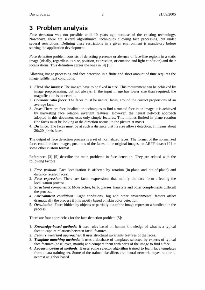
A graphic of the data (Graph 1) shows that the performance stands at the same level when it reachs 45 dimensions (about 0.001 PCAminp) and the minimun is got when using 20 hidden neurons and 13 dimensions: 0.49 (marked with yellow in Table 3). Performance starts to grow when dimensions are below 10 (about 0.004 PCAminp).

Grayscale Graphic

0

0.2

0.4

0.6

0.8

1

1.2

1.4

1.6

400 98 45 27 20 16 14 13 11 10 10

Dimensions

Test

dat

aset

MSE

5 neurons 10 neurons 15 neurons 20 neurons 25 neurons

Graph 1: Grayscale test dataset MSE versus Dimensions

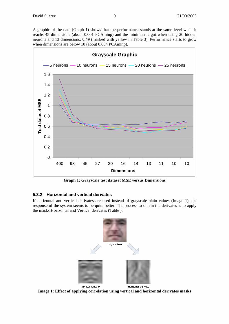
5.3.2 Horizontal and vertical derivates If horizontal and vertical derivates are used instead of grayscale plain values (Image 1), the response of the system seems to be quite better. The process to obtain the derivates is to apply the masks Horizontal and Vertical derivates (Table ).

Image 1: Effect of applying correlation using vertical and horizontal derivates masks


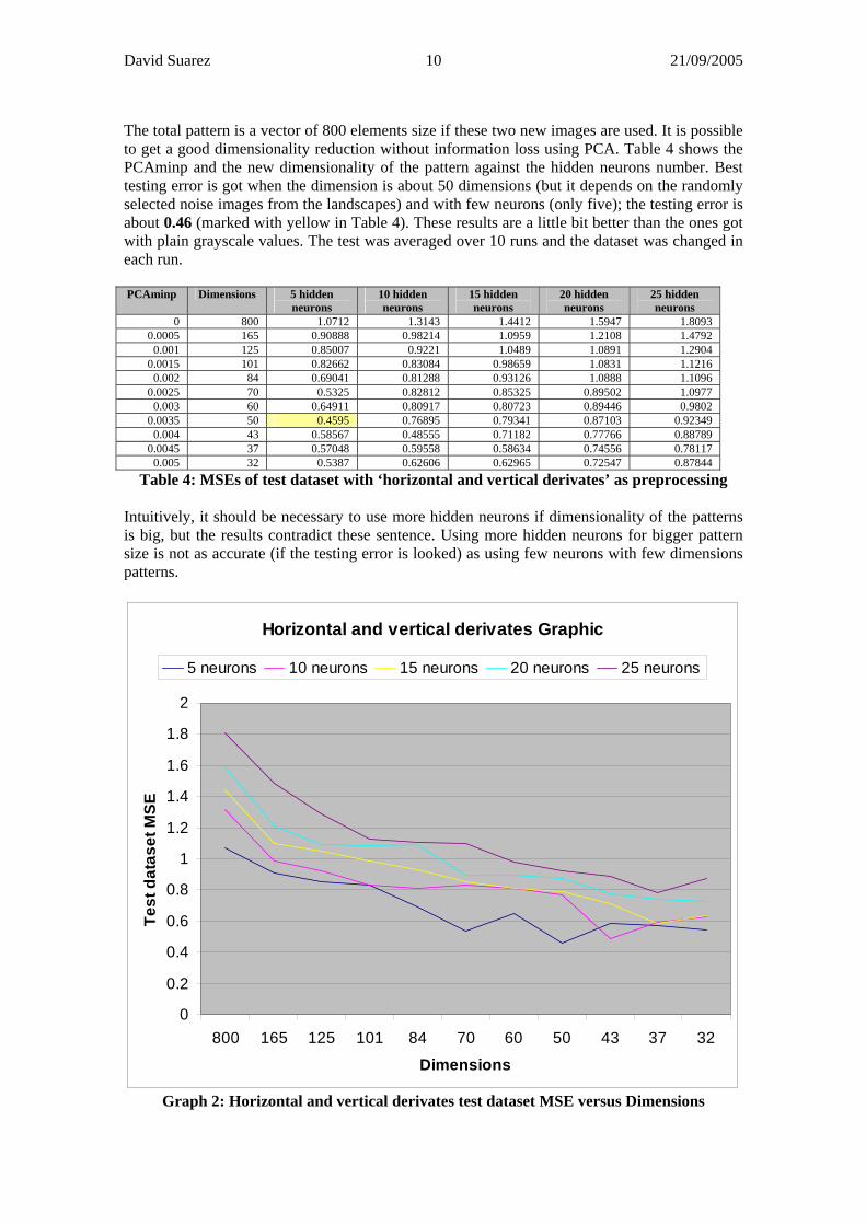
The total pattern is a vector of 800 elements size if these two new images are used. It is possible to get a good dimensionality reduction without information loss using PCA. Table 4 shows the PCAminp and the new dimensionality of the pattern against the hidden neurons number. Best testing error is got when the dimension is about 50 dimensions (but it depends on the randomly selected noise images from the landscapes) and with few neurons (only five); the testing error is about 0.46 (marked with yellow in Table 4). These results are a little bit better than the ones got with plain grayscale values. The test was averaged over 10 runs and the dataset was changed in each run. PCAminp Dimensions 5 hidden


15 hidden neurons

20 hidden neurons

25 hidden neurons

0 800 1.0712 1.3143 1.4412 1.5947 1.8093 0.0005 165 0.90888 0.98214 1.0959 1.2108 1.4792

0.001 125 0.85007 0.9221 1.0489 1.0891 1.2904 0.0015 101 0.82662 0.83084 0.98659 1.0831 1.1216

0.002 84 0.69041 0.81288 0.93126 1.0888 1.1096 0.0025 70 0.5325 0.82812 0.85325 0.89502 1.0977

0.003 60 0.64911 0.80917 0.80723 0.89446 0.9802 0.0035 50 0.4595 0.76895 0.79341 0.87103 0.92349

0.004 43 0.58567 0.48555 0.71182 0.77766 0.88789 0.0045 37 0.57048 0.59558 0.58634 0.74556 0.78117

0.005 32 0.5387 0.62606 0.62965 0.72547 0.87844 Table 4: MSEs of test dataset with ‘horizontal and vertical derivates’ as preprocessing

Intuitively, it should be necessary to use more hidden neurons if dimensionality of the patterns is big, but the results contradict these sentence. Using more hidden neurons for bigger pattern size is not as accurate (if the testing error is looked) as using few neurons with few dimensions patterns.

Horizontal and vertical derivates Graphic

0

0.2

0.4

0.6

0.8

1

1.2

1.4

1.6

1.8

2

800 165 125 101 84 70 60 50 43 37 32

Dimensions

Test

dat

aset

MSE


Graph 2: Horizontal and vertical derivates test dataset MSE versus Dimensions


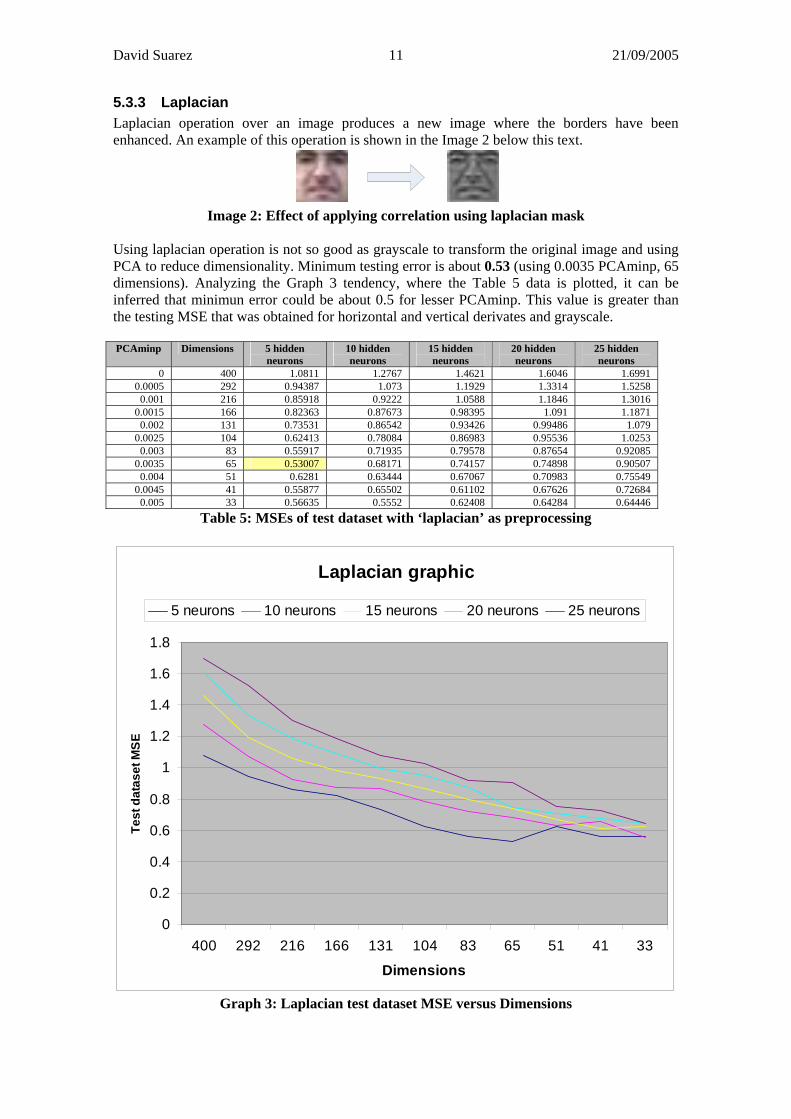
5.3.3 Laplacian Laplacian operation over an image produces a new image where the borders have been enhanced. An example of this operation is shown in the Image 2 below this text.

Image 2: Effect of applying correlation using laplacian mask

Using laplacian operation is not so good as grayscale to transform the original image and using PCA to reduce dimensionality. Minimum testing error is about 0.53 (using 0.0035 PCAminp, 65 dimensions). Analyzing the Graph 3 tendency, where the Table 5 data is plotted, it can be inferred that minimun error could be about 0.5 for lesser PCAminp. This value is greater than the testing MSE that was obtained for horizontal and vertical derivates and grayscale. PCAminp Dimensions 5 hidden


15 hidden neurons

20 hidden neurons

25 hidden neurons

0 400 1.0811 1.2767 1.4621 1.6046 1.6991 0.0005 292 0.94387 1.073 1.1929 1.3314 1.5258

0.001 216 0.85918 0.9222 1.0588 1.1846 1.3016 0.0015 166 0.82363 0.87673 0.98395 1.091 1.1871

0.002 131 0.73531 0.86542 0.93426 0.99486 1.079 0.0025 104 0.62413 0.78084 0.86983 0.95536 1.0253

0.003 83 0.55917 0.71935 0.79578 0.87654 0.92085 0.0035 65 0.53007 0.68171 0.74157 0.74898 0.90507

0.004 51 0.6281 0.63444 0.67067 0.70983 0.75549 0.0045 41 0.55877 0.65502 0.61102 0.67626 0.72684

0.005 33 0.56635 0.5552 0.62408 0.64284 0.64446 Table 5: MSEs of test dataset with ‘laplacian’ as preprocessing

Laplacian graphic

0

0.2

0.4

0.6

0.8

1

1.2

1.4

1.6

1.8

400 292 216 166 131 104 83 65 51 41 33

Dimensions

Test

dat

aset

MSE


Graph 3: Laplacian test dataset MSE versus Dimensions


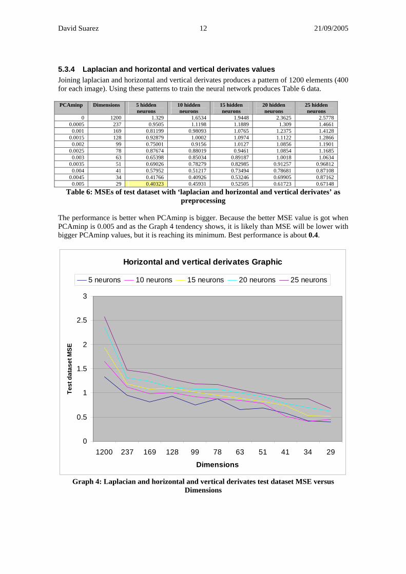
5.3.4 Laplacian and horizontal and vertical derivates values Joining laplacian and horizontal and vertical derivates produces a pattern of 1200 elements (400 for each image). Using these patterns to train the neural network produces Table 6 data. PCAminp Dimensions 5 hidden


15 hidden neurons

20 hidden neurons

25 hidden neurons

0 1200 1.329 1.6534 1.9448 2.3625 2.5778 0.0005 237 0.9505 1.1198 1.1889 1.309 1.4661

0.001 169 0.81199 0.98093 1.0765 1.2375 1.4128 0.0015 128 0.92879 1.0002 1.0974 1.1122 1.2866

0.002 99 0.75001 0.9156 1.0127 1.0856 1.1901 0.0025 78 0.87674 0.88019 0.9461 1.0854 1.1685

0.003 63 0.65398 0.85034 0.89187 1.0018 1.0634 0.0035 51 0.69026 0.78279 0.82985 0.91257 0.96812

0.004 41 0.57952 0.51217 0.73494 0.78681 0.87108 0.0045 34 0.41766 0.40926 0.53246 0.69905 0.87162

0.005 29 0.40323 0.45931 0.52505 0.61723 0.67148 Table 6: MSEs of test dataset with ‘laplacian and horizontal and vertical derivates’ as

preprocessing The performance is better when PCAminp is bigger. Because the better MSE value is got when PCAminp is 0.005 and as the Graph 4 tendency shows, it is likely than MSE will be lower with bigger PCAminp values, but it is reaching its minimum. Best performance is about 0.4.

Horizontal and vertical derivates Graphic

0

0.5

1

1.5

2

2.5

3

1200 237 169 128 99 78 63 51 41 34 29

Dimensions

Test

dat

aset

MSE


Graph 4: Laplacian and horizontal and vertical derivates test dataset MSE versus

Dimensions


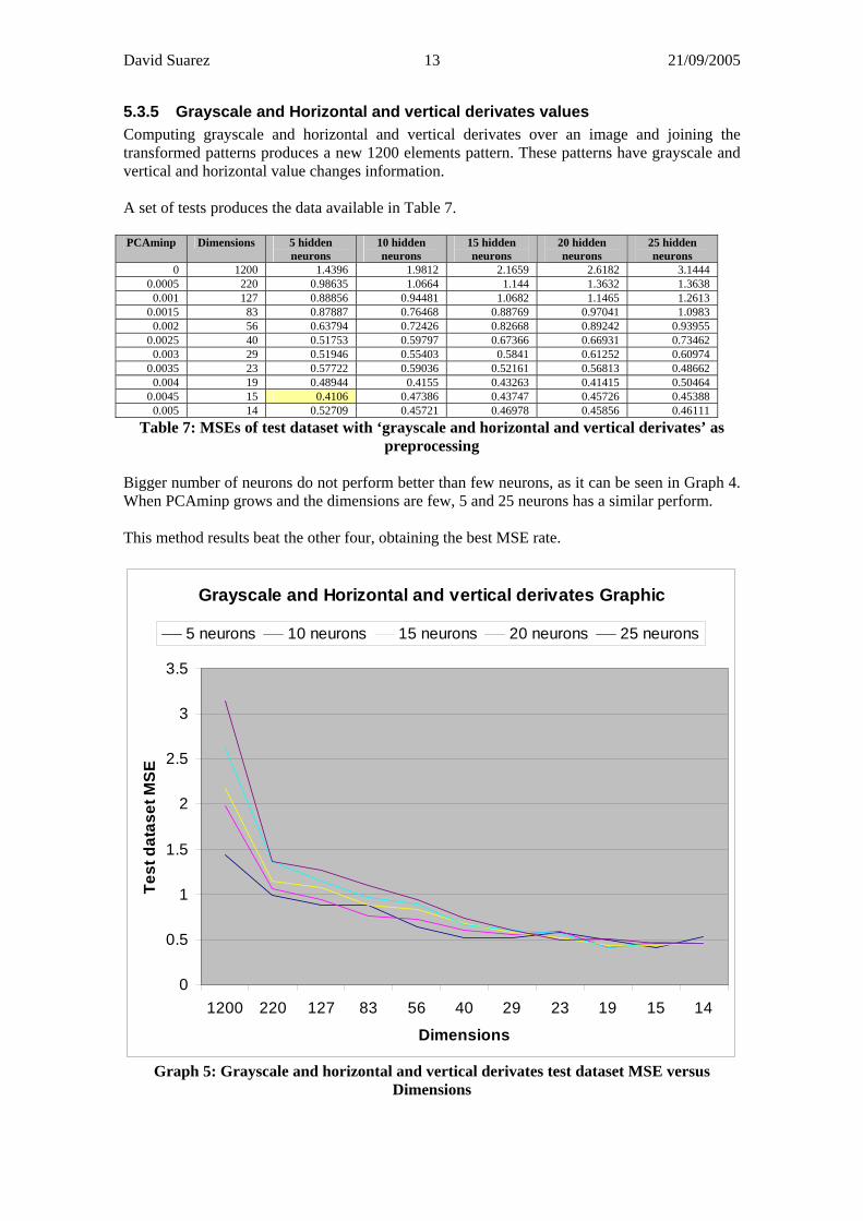
5.3.5 Grayscale and Horizontal and vertical derivates values Computing grayscale and horizontal and vertical derivates over an image and joining the transformed patterns produces a new 1200 elements pattern. These patterns have grayscale and vertical and horizontal value changes information. A set of tests produces the data available in Table 7. PCAminp Dimensions 5 hidden


15 hidden neurons

20 hidden neurons

25 hidden neurons

0 1200 1.4396 1.9812 2.1659 2.6182 3.1444 0.0005 220 0.98635 1.0664 1.144 1.3632 1.3638

0.001 127 0.88856 0.94481 1.0682 1.1465 1.2613 0.0015 83 0.87887 0.76468 0.88769 0.97041 1.0983

0.002 56 0.63794 0.72426 0.82668 0.89242 0.93955 0.0025 40 0.51753 0.59797 0.67366 0.66931 0.73462

0.003 29 0.51946 0.55403 0.5841 0.61252 0.60974 0.0035 23 0.57722 0.59036 0.52161 0.56813 0.48662

0.004 19 0.48944 0.4155 0.43263 0.41415 0.50464 0.0045 15 0.4106 0.47386 0.43747 0.45726 0.45388

0.005 14 0.52709 0.45721 0.46978 0.45856 0.46111 Table 7: MSEs of test dataset with ‘grayscale and horizontal and vertical derivates’ as

preprocessing Bigger number of neurons do not perform better than few neurons, as it can be seen in Graph 4. When PCAminp grows and the dimensions are few, 5 and 25 neurons has a similar perform. This method results beat the other four, obtaining the best MSE rate.

Grayscale and Horizontal and vertical derivates Graphic

0

0.5

1

1.5

2

2.5

3

3.5

1200 220 127 83 56 40 29 23 19 15 14

Dimensions

Test

dat

aset

MSE


Graph 5: Grayscale and horizontal and vertical derivates test dataset MSE versus

Dimensions


5.3.6 Final comments It can be seen the best results are got when the PCA minimum information percentage is high, deprecating several dimensions from the initial pattern. The limit to stop increasing PCaminp in grayscale, horizontal and vertical and laplacian patterns is low; the MSE starts to grow about 0.004 PCAminp. PCA works better and PCaminp can reach 0.005 in the other two methods (union of two methods). However, the grayscale and horizontal and vertical derivates graph shows that higher values of PCAminp improve the performance asymptotically; but for 0.5% the number of dimensions is only 14. It can be inferred that this behavior is reaching its limit; using a bigger PCAminp reduces so much dataset dimension that about 0.01 PCAminp, the resulting dataset is size 0. Comparing the five approaches, the pattern consisting on horizontal, vertical and grayscale information works better, but only a little bit more than horizontal, vertical and laplacian data consisting patterns. Laplacian values are not good enough to allow face detection.

6 Results This section shows some results that can be obteined using this approach. The neural network parameters are summarized in Table 8. It was trained two times before obtaining that performance value. Dataset 54 face like regions 27 for training dataset 14 for testing dataset 13 for validation

2160 noise patterns 1080 for training dataset 540 for testing dataset 540 for validation dataset

299 no face-like regions 150 for training dataset 50 for testing dataset 49 for validation PCA minimum information percentage 0.0045 Hidden Neurons 5 Results 0.39 Testing performance

Table 8: Training parameters Face detection process parameters are in Table 9. Face Threshold 0.95 Clustering maximum distance 11

Table 9: Running parameters


6.1 Test 1: Faces from the training dataset The image is 512x384 pixels. Faces are about 20x20 pixels size (but the image was not expressly resized to allow good face reduction). The subjects’ faces belong to the training dataset faces. First image is input image (Image 3); the second one (Image 4) has only skin regions and third one shows the face-like regions (Image 5).

Image 3: Training dataset faces

Image 4: Image skin regions

There are several false positives in this image. The flowers in the bottom border and the paintings in the left-top corner are detected as face-like regions. This fact is because deficient training process. The neural network cannot classify these regions into the correct class. Increasing the number of noise and no face-like regions in the training dataset could improve the results


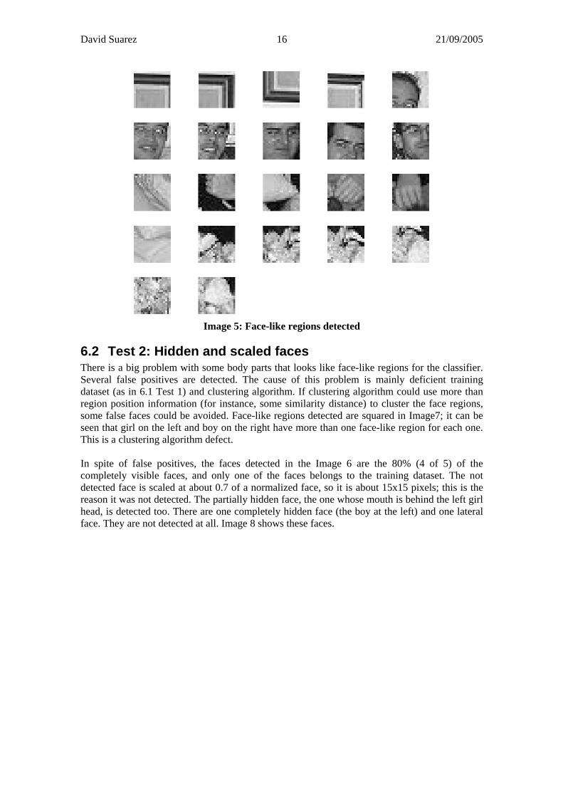
Image 5: Face-like regions detected

6.2 Test 2: Hidden and scaled faces There is a big problem with some body parts that looks like face-like regions for the classifier. Several false positives are detected. The cause of this problem is mainly deficient training dataset (as in 6.1 Test 1) and clustering algorithm. If clustering algorithm could use more than region position information (for instance, some similarity distance) to cluster the face regions, some false faces could be avoided. Face-like regions detected are squared in Image7; it can be seen that girl on the left and boy on the right have more than one face-like region for each one. This is a clustering algorithm defect.

In spite of false positives, the faces detected in the Image 6 are the 80% (4 of 5) of the completely visible faces, and only one of the faces belongs to the training dataset. The not detected face is scaled at about 0.7 of a normalized face, so it is about 15x15 pixels; this is the reason it was not detected. The partially hidden face, the one whose mouth is behind the left girl head, is detected too. There are one completely hidden face (the boy at the left) and one lateral face. They are not detected at all. Image 8 shows these faces.


Image 6: Hidden and scaled faces image

Image 7: Detail of face-like regions detected on their position on the image



6.3 Test 3: Slightly rotated faces Image 9 in test 3 was resized so faces in the image were about 20x20 pixels. The subjects’ faces were not in the training dataset, and they are slightly rotated so detection should be less accurate.

Image 9: Slightly rotated faces

Graph 6 shows face-like regions founded and central point of the clustered faces (Face 1 and Face 2) corresponding to the girl and the boy (they can be seen at Image 10). Boy’s face is a little bit shift. It is probably because some no face-like regions were dectected as face-like regions: the two ones about 100 - 120 at the X axis and 100 – 102 at the Y axis. This mistake makes clustering algorithm to select them as face-like regions for Face 2 set and using their position to average the Face 2 position.

Clusterizing algorithm

100

102

104

106

108

110

112

0 20 40 60 80 100 120 140 160

X

Y

Face-like regionsFace 1Face 2

Graph 6: Clustering algorithm result



7 Conclusions Artificial neural networks are a biological based method; however, the whole face detection process proposed is not biologically inspired. Several non biological techniques have been used to reduce problem complexity. In addition, the way the neural network has been used is not the way the human being vision seems to work. Human vision detects faces in a wide range of situations and it makes use of non-visual information. The scope of the paper has been limited to face detection in controlled pose, light and scale situations. Lighter, distort or big (and small) faces in the images are not detected. Avoiding the problems involves developing an automatic features detection system to detect face characteristics in the images, grouping them and recognize their struct as a face struct. Rotation and scaling invariant can be accomplished following this schema. Independently of other approaches, there is a problem related to PCA linear nature. Non linear relations between variables are not captured. Curvilinear Component Analysis could fix it. In addition, neural network training should be complete; more face and noise patterns on the datasets could make the network detect with better accuracy. Finally, clustering algorithm could take information from image composition (characteristics) and not only from face positions to cluster the face-like images. Using more noise regions could help avoiding false positives. This approach could be good if it is used in a static place. For instance, at the entrance of a building, where faces of the people are frontally captured. Neural network can be trained to detect background regions as no face-like images so false positives will be reduced. Using it as a general face detector is far of being useful because its high false positive rate.

8 References [1] Darío de Miguel Benito. (2005). Detección automática del color de la piel en imágenes. Proyecto de Fin de

Carrera. Universidad Rey Juan Carlos. 14.09.05. http://www.escet.urjc.es/~jjpantrigo/documentos/MemoriaPielFeb05.pdf

[2] Weka Project. University of Waikato. Attribute-Relation File Format (ARFF).

14.09.05. http://www.cs.waikato.ac.nz/~ml/weka/arff.html [3] Ming-Hsuan Yang. (2004). Recent Advances in Face Detection. IEEE ICPR 2004 Tutorial, Cambridge,

United Kingdom, August 22, 2004. 14.09.05. http://vision.ai.uiuc.edu/mhyang/papers/icpr04_tutorial.pdf [4] Overview of face detection algorithms (proposal). Tao Wang, CMPUT 615. 14.09.05. http://www.ee.ualberta.ca/~xiang/proposal2 [5] Ming-Hsuan Yang, David J. Kriegman, Narendra Ahuja. (2002). Detecting Faces in Images: A Survey.

IEEE Transactions On Pattern Analysis And Machine Intelligence, Vol. 24, No. 1, January 2002. 14.09.05. http://vision.ai.uiuc.edu/mhyang/papers/pami02a.pdf


[6] Henry A. Rowley, Shumeet Baluja, Takeo Kanade. (1998). Neural Network-Based Face Detection. IEEE

Transactions on Pattern Analysis and Machine Intelligence, Vol. 20, No. 1, January, 1998, pp. 23-38. [7] Emiliano Acosta, Luis Torres, Alberto Albiol, Edward Delp. (2002). An Automatic Face Detection And

Recognition System For Video Indexing Applications. 14.09.05. http://gps-tsc.upc.es/GTAV/Torres/Publications/ICASSP02_Acosta_Torres_Albiol_Delp.pdf

[8] Tae-Kyun Kim, Sung-Uk Lee, Jong-Ha Lee, Seok-Cheol Kee, Sang-Ryong Kim. (2002). Integrated

Approach of Multiple Face Detection for Video Surveillance. Pattern Recognition, 2002. Proceedings. 16th International Conference on Publication. Vol.2, pp. 394- 397. 14.09.05. http://iris.usc.edu/~slee/05_2_20.PDF

[9] B. Heisele, T. Serre, M. Pontil, T. Poggio. (2001). Component-based Face Detection.

14.09.05. http://cbcl.mit.edu/projects/cbcl/publications/ps/cvpr2001-1.pdf [10] Matthias Rätsch, Sami Romdhani, Thomas Vetter. (2004). Efficient Face Detection by a Cascaded Support

Vector Machine using Haar-like Features. 14.09.05. http://eprints.pascal-network.org/archive/00000931/01/dagm04.pdf

[11] Ming-Jung Seow, Deepthi Valaparla, Vijayan K. Asari. (2003). Neural Network Based Skin Color Model

for Face Detection. IEEE Computer Society, 32nd Applied Imagery Pattern Recognition Workshop, p. 141. 14.09.05. http://doi.ieeecomputersociety.org/10.1109/AIPR.2003.1284262

[12] C.Chen, S.P. Chiang. (1997). Detection of human faces in colour images. Vision, Image and Signal

Processing, IEEE Proceedings December 1997, Vol. 144, Issue: 6, pp 384-388. [13] Diedrick Marius, Sumita Pennathur, and Klint Rose. Face Detection Using Color Thresholding, and

Eigenimage Template Matching. 14.09.05. http://www.stanford.edu/class/ee368/Project_03/Project/reports/ee368group15.pdf

[14] Jaakko Hollmen. Principal Componen Analysis.

14.09.05. http://www.cis.hut.fi/~jhollmen/dippa/node29.html

[15] Henry A. Rowley, Shumeet Baluja, Takeo Kanade. (1998). Rotation Invariant Neural Network-Based Face Detection. 1998 IEEE Computer Society Conference on Computer Vision and Pattern Recognition (CVPR'98) p. 38. 14.09.05. http://doi.ieeecomputersociety.org/10.1109/CVPR.1998.698585

backpropagation neural network based face detection in...

Documents