Introduction Proposed Approach Empirical Results Concluding Remarks References

Bagging-Clustering Methods to Forecast TimeSeries

Tiago DantasFernando Cyrino

Pontifical Catholic University of Rio de Janeiro,Brazil

ISF 2017, Cairns-Australia, June 25-28

June 28, 2017

Tiago Dantas, Fernando Cyrino ISF 2017

Introduction Proposed Approach Empirical Results Concluding Remarks References

Introduction

I Cordeiro and Neves (2009) and Bergmeir et al. (2016), haveproposed new ways to generate forecasts using a very popularMachine Learning technique, called Bagging (BootstrapAggregating), proposed by Breiman (1996), in combinationwith Exponential Smoothing methods to improve forecastaccuracy

I The main idea is to use Bootstrap to generate an ensemble offorecasts that is combined into one single output

Tiago Dantas, Fernando Cyrino ISF 2017

Introduction Proposed Approach Empirical Results Concluding Remarks References

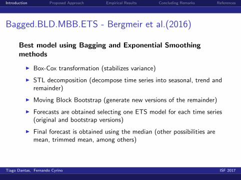
Bagged.BLD.MBB.ETS - Bergmeir et al.(2016)

Best model using Bagging and Exponential Smoothingmethods

I Box-Cox transformation (stabilizes variance)

I STL decomposition (decompose time series into seasonal, trend andremainder)

I Moving Block Bootstrap (generate new versions of the remainder)

I Forecasts are obtained selecting one ETS model for each time series(original and bootstrap versions)

I Final forecast is obtained using the median (other possibilities aremean, trimmed mean, among others)

Tiago Dantas, Fernando Cyrino ISF 2017

Introduction Proposed Approach Empirical Results Concluding Remarks References

Bagged.BLD.MBB.ETS - Bergmeir et al.(2016)

Tiago Dantas, Fernando Cyrino ISF 2017

Introduction Proposed Approach Empirical Results Concluding Remarks References

Why Bagging tends to work

The Mean Squared Forecast Error (MSFE) can be decomposedinto three terms:

MSFE = Var(yt+1|t) + bias(yt+1|t)2 + Var(yt+1|t)

Tiago Dantas, Fernando Cyrino ISF 2017

Introduction Proposed Approach Empirical Results Concluding Remarks References

Why Bagging tends to work

The average forecast over the Bootstrap samples can be written as:

yt+1|t = 1B

B∑i=1

y∗(i)t+1|t

where the tilde indicates Bagging forecast and B is the totalnumber of Bootstrap samples.

Tiago Dantas, Fernando Cyrino ISF 2017

Introduction Proposed Approach Empirical Results Concluding Remarks References

Why Bagging tends to work

bias(yt+1|t) = 1B

B∑i=1

bias(y∗(i)t+1|t)

I Note that unbiased Bootstrapped versions lead to a relativelyunbiased ensemble

Tiago Dantas, Fernando Cyrino ISF 2017

Introduction Proposed Approach Empirical Results Concluding Remarks References

Why Bagging tends to work

Var(yt+1|t) = 1B2

B∑i=1

Var(y∗(i)t+1|t) + 1B2

∑i 6=i ′

Cov [y∗(i)t+1|t , y∗(i ′)t+1|t ]

I Variance tends to be reduced

Tiago Dantas, Fernando Cyrino ISF 2017

Introduction Proposed Approach Empirical Results Concluding Remarks References

Why Bagging tends to work

I When applying Bagging and Exponential Smoothing whathappens is variance reduction

I If the variances are approximately equal and there is nocorrelation:

Var(yt+1|t) ≈ 1BVar(y∗(1)t+1|t)

Tiago Dantas, Fernando Cyrino ISF 2017

Introduction Proposed Approach Empirical Results Concluding Remarks References

Why Bagging tends to work

I Reducing covariance seems to be a good idea

Var(yt+1|t) = 1B2

B∑i=1

Var(y∗(i)t+1|t) + 1B2

∑i 6=i ′

Cov [y∗(i)t+1|t , y∗(i ′)t+1|t ]

I The proposed approach tries to use this idea in order toreduce forecast error

Tiago Dantas, Fernando Cyrino ISF 2017

Introduction Proposed Approach Empirical Results Concluding Remarks References

Proposed ApproachThe proposed approach can be divided in two parts:

1. Generation of Bootstrapped series - Algorithm developed byBergmeir et al. (2016)

2. The procedure to forecast and aggregate the series - Newdevelopments

Tiago Dantas, Fernando Cyrino ISF 2017

Introduction Proposed Approach Empirical Results Concluding Remarks References

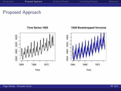
Proposed Approach

Generating bootstrapped series

I Bootstrapped series are generated in the same way asBagged.BLD.MBB.ETS

Tiago Dantas, Fernando Cyrino ISF 2017

Introduction Proposed Approach Empirical Results Concluding Remarks References

Algorithm 1 Generating bootstrapped series

1: procedure BOOTSTRAP(ts,num.boot)2: λ← BoxCox.lambda(ts,min=0,max=1)3: ts.bc← BoxCox(ts,λ = 1)4: if ts is seasonal then5: [trend seasonal remainder] ← stl(ts.bc)6: else7: seasonal ← 08: [trend,remainder] ← loess(ts.bc)9: end if10: recon.series[1] ← ts11: for i in 2 to num.boot do12: boot.sample[i] ← MBB(remainder)13: recon.series.bc[i] ← trend + seasonal +boot.sample[i]14: recon.series[i] ← InvBoxCox(recon.series.bc[i],λ)15: end for16: return recon.series17: end procedure

Tiago Dantas, Fernando Cyrino ISF 2017

Introduction Proposed Approach Empirical Results Concluding Remarks References

Proposed Approach

Tiago Dantas, Fernando Cyrino ISF 2017

Introduction Proposed Approach Empirical Results Concluding Remarks References

Proposed Approach

The procedure to forecast and aggregate the series

I the Proposed approach and Bagged.BLD.MBB.ETS differ inthe way the ensemble is constructed

I Bagged.BLD.MBB.ETS consider all of the Bootstrappedversions to make forecasts

I The proposed approach considers a less correlated group oftime series to make forecasts

Tiago Dantas, Fernando Cyrino ISF 2017

Introduction Proposed Approach Empirical Results Concluding Remarks References

Proposed Approach

I To create a less correlated ensemble, the proposal is togenerate clusters from the Bootstrapped versions

I Cluster procedures maximize similarity within the group andminimize it between them

I The expectation is that selecting series from different clusterswould lead to an ensemble less correlated and, therefore, lesscorrelated forecasts to be aggregated

Tiago Dantas, Fernando Cyrino ISF 2017

Introduction Proposed Approach Empirical Results Concluding Remarks References

Proposed Approach

I Partitioning Around Medoids Algorithm (PAM) and euclideandistance are used to create the clusters (fast algorithm andless sensible to outliers)

I The number of cluster can be defined using cross-validation orany other method (e.g. Silhouette Information)

Tiago Dantas, Fernando Cyrino ISF 2017

Introduction Proposed Approach Empirical Results Concluding Remarks References

Proposed Approach

Tiago Dantas, Fernando Cyrino ISF 2017

Introduction Proposed Approach Empirical Results Concluding Remarks References

Proposed Approach

Tiago Dantas, Fernando Cyrino ISF 2017

Introduction Proposed Approach Empirical Results Concluding Remarks References

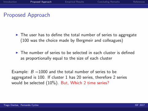
Proposed Approach

I The user has to define the total number of series to aggregate(100 was the choice made by Bergmeir and colleagues)

I The number of series to be selected in each cluster is definedas proportionally equal to the size of each cluster

Example: B =1000 and the total number of series to beaggregated is 100. If cluster 1 has 20 series, therefore 2 serieswould be selected (10%). But, Which 2 time series?

Tiago Dantas, Fernando Cyrino ISF 2017

Introduction Proposed Approach Empirical Results Concluding Remarks References

I A validation set is defined

I The time series with best results (sMAPE) in the validationset are the ones selected in each cluster

I The final forecast is obtained taking the median of theforecasts (other possibilities are the mean, trimmed mean)

Tiago Dantas, Fernando Cyrino ISF 2017

Introduction Proposed Approach Empirical Results Concluding Remarks References

Proposed Approach

Tiago Dantas, Fernando Cyrino ISF 2017

Introduction Proposed Approach Empirical Results Concluding Remarks References

MSE decompositionBagged.BLD.MBB.ETS (black) and the Proposed Approach (blue)- Forecast (up to 18 steps ahead) - Time series 1083 - M3competition

Tiago Dantas, Fernando Cyrino ISF 2017

Introduction Proposed Approach Empirical Results Concluding Remarks References

Empirical Results

I The proposed approach was validated on public available timeseries from the M3 competition (1428 monthly, 756 quarterlyand 645 yearly time series)

I The experiment was conducted using R and the majorly theforecast package (version 8.0)

I The results for Bagged.BLD.MBB.ETS were obtained usingbaggedETS()

Tiago Dantas, Fernando Cyrino ISF 2017

Introduction Proposed Approach Empirical Results Concluding Remarks References

Monthly data

Tiago Dantas, Fernando Cyrino ISF 2017

Introduction Proposed Approach Empirical Results Concluding Remarks References

Methods Rank sMAPE Mean sMAPE Median sMAPEProposed Approach 11.15 13.62 8.74Bagged.BLD.MBB.ETS 11.30 13.65 8.85THETA 11.53 13.89 8.92ForecastPro 11.56 13.90 8.81COMB S-H-D 12.54 14.47 9.37ForcX 12.76 14.47 9.21HOLT 12.78 15.79 9.28WINTER 13.06 15.93 9.30RBF 13.27 14.76 9.21AAM1 13.48 15.67 9.67DAMPEN 13.48 14.58 9.44AutoBox2 13.60 15.73 9.28B-J auto 13.69 14.80 9.32AutoBox1 13.69 15.81 9.27SMARTFCS 13.82 15.01 9.52Flors-Pearc2 13.84 15.19 9.61AAM2 13.85 15.94 9.62Auto-ANN 13.91 15.03 9.62PP-Autocast 14.13 15.33 9.90ARARMA 14.20 15.83 9.80AutoBox3 14.21 16.59 9.40Flors-Pearc1 14.54 15.99 9.96THETAsm 14.58 15.38 9.65ROBUST-Trend 14.79 18.93 9.73SINGLE 15.22 15.30 10.03NAIVE2 16.04 16.89 10.12

Tiago Dantas, Fernando Cyrino ISF 2017

Introduction Proposed Approach Empirical Results Concluding Remarks References

Quarterly data

Tiago Dantas, Fernando Cyrino ISF 2017

Introduction Proposed Approach Empirical Results Concluding Remarks References

Methods Rank sMAPE Mean sMAPE Median sMAPETHETA 11.39 8.96 5.37COMB S-H-D 12.18 9.22 5.32ROBUST-Trend 12.44 9.79 5.00DAMPEN 12.66 9.36 5.59PP-Autocast 12.81 9.39 5.26ForcX 12.86 9.54 5.62Bagged.BLD.MBB.ETS 12.96 9.80 5.81B-J auto 13.16 10.26 5.69ForecastPro 13.20 9.82 5.84Proposed Approach 13.24 9.89 5.82HOLT 13.27 10.94 5.71RBF 13.30 9.57 5.67AutoBox2 13.38 10.00 5.59WINTER 13.38 10.84 5.71Flors-Pearc1 13.48 9.95 5.61ARARMA 13.49 10.19 6.11Auto-ANN 13.89 10.20 6.28THETAsm 14.18 9.82 5.65AAM1 14.25 10.16 6.36SMARTFCS 14.27 10.15 5.71Flors-Pearc2 14.30 10.43 6.22AutoBox3 14.38 11.19 6.15AAM2 14.41 10.26 6.44SINGLE 14.66 9.72 6.18AutoBox1 14.69 10.96 6.14NAIVE2 14.80 9.95 6.18

Tiago Dantas, Fernando Cyrino ISF 2017

Introduction Proposed Approach Empirical Results Concluding Remarks References

Yearly data

Tiago Dantas, Fernando Cyrino ISF 2017

Introduction Proposed Approach Empirical Results Concluding Remarks References

Methods Rank sMAPE Mean sMAPE Median sMAPEForcX 11.15 16.48 11.34RBF 11.46 16.42 10.74AutoBox2 11.48 16.59 11.31Flors-Pearc1 11.57 17.21 10.72THETA 11.58 16.97 11.25ForecastPro 11.73 17.27 11.05ROBUST-Trend 11.81 17.03 11.30PP-Autocast 11.87 17.13 10.83Bagged.BLD.MBB.ETS 11.89 17.40 11.20DAMPEN 11.92 17.36 10.95COMB S-H-D 11.99 17.07 11.68Proposed Approach 12.21 17.56 11.42SMARTFCS 12.38 17.71 11.83HOLT 12.64 20.02 11.77WINTER 12.64 20.02 11.77Flors-Pearc2 13.02 17.84 12.55ARARMA 13.03 18.36 11.35B-J auto 13.04 17.73 11.70Auto-ANN 13.32 18.57 13.08AutoBox3 13.52 20.88 12.89THETAsm 13.55 17.92 12.21AutoBox1 13.82 21.59 12.75NAIVE2 14.16 17.88 12.37SINGLE 14.21 17.82 12.44

Tiago Dantas, Fernando Cyrino ISF 2017

Introduction Proposed Approach Empirical Results Concluding Remarks References

Concluding Remarks

I This proposed approach make forecasts combining Bagging,Exponential Smoothing and Cluster methods

I The empirical results demonstrate the approach was capableof generating highly accurate forecasts for monthly time series

I The so far, not explicitly addressed, covariance effect on thecombination of Bagging and Exponential Smoothing, isprobably resposible for reducing the forecast error

I The method doesn’t seem to work well on short time series(such as the case of yearly and quarterly time series from theM3 competition)

Tiago Dantas, Fernando Cyrino ISF 2017

Introduction Proposed Approach Empirical Results Concluding Remarks References

Concluding Remarks

Future work

I Other weighting schemes for selected series

I Other decomposition and forecasting methods

Tiago Dantas, Fernando Cyrino ISF 2017

Introduction Proposed Approach Empirical Results Concluding Remarks References

Thank You!t.mendesdantas@gmail.com

Tiago Dantas, Fernando Cyrino ISF 2017

Introduction Proposed Approach Empirical Results Concluding Remarks References

ReferencesBergmeir, C., Hyndman, R.J., Benitez,J.M. (2016). Baggingexponential smoothing methods using STL decomposition andBox-Cox transformation.International Journal of Forecasting,32(2), 303-312.

Breiman, L. (1996). Bagging Predictors.Machine Learning, 24,123-140.

Cordeiro, C.,Neves,M. (2009). Forecasting time series withBOOT.EXPOS procedure. REVSTAT-Statistical Journal, 7(2),135-149.

Liao, T.W. (2005). Clustering of time series data - asurvey.Journal of Pattern Recognition, 38(11), 1857-1874.

Monteiro,P.,Vilar, J.A. (2016). TSclust: An R Package for TimeSeries Clustering.Journal of Statistical Software, 62(1), 1-43.

Tiago Dantas, Fernando Cyrino ISF 2017