baker 08hqag0115 final report - stanford universitybakerjw/publications/baker... · pi: jack baker...
TRANSCRIPT
1
FINAL TECHNICAL REPORT
AWARD NUMBER: 08HQAG0115
Ground Motion Target Spectra for Structures Sensitive to Multiple Periods of Excitation: Conditional Mean Spectrum Computation Using Multiple Ground Motion Prediction
Models
PI: Jack Baker Report co-author: Ting Lin (Stanford University) Dept. of Civil & Environmental Engineering
Yang & Yamasaki Environment & Energy Building 473 Via Ortega, Room 283 Stanford CA 94305-4020
650-725-2573 (phone) 650-723-7514 (fax)
February 2009
Research supported by the U. S. Geological Survey (USGS), Department of Interior, under USGS award number 08HQAG0115. The views and conclusions contained in this document are those of the authors and should not be interpreted as necessarily representing the official policies, either expressed or implied, of the U. S. Government.

2
Abstract
Probabilistic seismic hazard analysis (PSHA) combines the probabilities of all earthquake
scenarios with different magnitudes and distances with predictions of the resulting ground
motion intensity, in order to compute seismic hazard at a site. PSHA also incorporates
uncertainties in those ground motion predictions, by considering multiple ground motion
prediction (“attenuation”) models (GMPMs). Current ground motion selection uses the
information from earthquake scenarios without considering multiple GMPMs. This paper
describes ways to incorporate multiple GMPMs, using refinements to disaggregation and
Conditional Mean Spectrum (CMS).
CMS, a new target spectrum proposed for ground motion selection, utilizes the
correlation of spectral acceleration (Sa) across periods to compute the “expected” or mean
spectrum given a target Sa at a single period of interest; we use a simplified site example to
illustrate CMS computation incorporating multiple GMPMs. Disaggregation of GMPMs plays
an important role in CMS computation, in a similar way as assigned weights of GMPMs do in
PSHA computation. Just as the disaggregation of magnitude and distance identifies the relative
contribution of each earthquake scenario to exceedance of a given Sa level, the disaggregation of
GMPMs tells us the probability that the exceedance of that Sa level was predicted by a specific
GMPM. We can further extend disaggregation to other ground motion parameters, such as
earthquake fault types, to more accurately represent the parameters that contribute most to Sa
values of engineering interest.

3
Table of Contents Abstract ........................................................................................................................................... 2
1 Introduction ............................................................................................................................. 4
2 Disaggregation Using Multiple Ground Motion Prediction Models ...................................... 5
2.1 Parameters ........................................................................................................................ 5
2.2 Probabilistic Seismic Hazard Analysis ............................................................................ 6
2.3 Disaggregation of Magnitude. Distance, and Epsilon ...................................................... 7
2.4 Disaggregation of Ground Motion Prediction Models ..................................................... 8
2.5 Disaggregation of Other Parameters ................................................................................ 9
3 Conditional Mean Spectrum Computation ............................................................................. 9
4 Calculation Procedure and Site Application ......................................................................... 11
4.1 Description of Site and Events ....................................................................................... 11
4.2 Disaggregation of Events ............................................................................................... 12
4.3 Disaggregation of Ground Motion Prediction Models ................................................... 13
4.4 Disaggregation of Magnitude, Distance, and Epsilon .................................................... 13
4.5 Conditional Mean Spectrum Computation Using Two Approaches .............................. 15
5 Discussion and Conclusions ................................................................................................. 18
Acknowledgments......................................................................................................................... 19

4
1 Introduction
Performance of structures during and after earthquakes is critical to public safety and
societal functionality. Performance-based earthquake engineering aims to improve seismic
design and analysis of structures through risk analysis. In performance-based earthquake
engineering, we input ground motion into a structural model to predict structural response such
as maximum interstory drift ratio. Subsequently, we use structural response to categorize
damage states and estimate losses in terms of dollars, down time and fatalities, in order to
quantify performance of structures under earthquakes.
To mitigate earthquake risk, we must first identify ground motion hazard, through
probabilistic seismic hazard analysis (PSHA). PSHA combines the probabilities of all
earthquake scenarios with different magnitudes and distances in order to compute seismic hazard
at a site. PSHA also incorporates uncertainties in ground motion prediction, by considering
multiple ground motion prediction models (GMPMs), formerly known as attenuation equations
(e.g., Abrahamson and Silva 1997). GMPMs have inputs such as magnitude and distance, and
outputs in terms of logarithmic mean and standard deviation of spectral acceleration (Sa). When
multiple GMPMs are present, we typically use a logic tree to assign a weight to each GMPM.
PSHA then estimates seismic hazard at a site incorporating uncertainties from earthquake
scenario and GMPMs.
Ground motion selection is a key step in defining the seismic load input to structural
analysis. Current ground motion selection uses the information from earthquake scenarios
without considering multiple GMPMs. While PSHA computes the total seismic hazard using
total probability, its reverse process--PSHA disaggregation--computes the relative contribution
of earthquake parameters to the total hazard using conditional probability. Current ground
motion selection utilizes disaggregation results of magnitude and distance to identify causal
events for a given Sa value corresponding to a return period. In this paper we consider ways to
incorporate multiple GMPMs into ground motion selection techniques using refinements to
PSHA disaggregation.
Ground motion selection often involves specification of a target spectrum. Baker (2005)
proposed a target spectrum termed the conditional mean spectrum (CMS), which shows several
improvements over the commonly used uniform hazard spectrum (UHS). For the UHS, the
probability of Sa exceedance is the same across all periods. But observed spectra rarely look like

5
a UHS, for several reasons. Different frequency regions of the UHS are often associated with
different earthquake events. The UHS is also typically associated with above-average Sa values
for the causal earthquake event, and due to imperfect correlation of Sa values it is unlikely that
this above-average condition will occur at all periods simultaneously. Thus, no single ground
motion is likely to produce a response spectrum as high as that of the UHS. To account for the
variation of causal earthquake events and Sa values for a given causal event, the CMS makes use
of the correlation of Sa across different periods. CMS answers the question, “Given a Sa at the
first-mode period of a structure, what will be the expected Sa at other periods?” The procedure
for performing this calculation will be described later. The CMS calculations utilizes the
magnitude, distance and “epsilon” values obtained from disaggregation, but it also requires the
user to choose a GMPM for the calculation. With additional insights into the relative
contribution of GMPMs from this new disaggregation refinement, we can more effectively
choose appropriate GMPMs for CMS calculations, and thus overcome a practical challenge to
implementing the CMS in performance based earthquake engineering.
2 Disaggregation Using Multiple Ground Motion Prediction Models
Computation of the Conditional Mean Spectrum requires disaggregation to identify the
causal parameters. Since multiple Ground Motion Prediction Models are typically used in
practice for Probabilistic Seismic Hazard Analysis, PSHA disaggregation can be extended to
include multiple GMPMs. To demonstrate, we use the models and weights specified by the
United States Geological Survey (USGS) for the Western US non-extensional tectonic areas
(Frankel et al. 2002): Abrahamson and Silva (1997), Boore et al.(1997), Campbell (1997)1, and
Sadigh et al.(1997)2, with equal weights.
2.1 Parameters
Different GMPMs require different input parameters. This variation presents challenges
for the disaggregation process. The parameters used in each model are shown in Table 1. The
1 Campbell (1997) was used in the proposed method instead of Campbell and Bozorgnia (2003) in the USGS method because the former was previously programmed and thus readily available. We believe the differences between the two models are minor, and will compare and verify these differences in the future. 2 We have modified the Sadigh et al. model to correct an error in the prediction equation in Table 2 in the original publication. The Abrahamson and Silva model has also been modified to correct some errors in the original publication. The ground motion prediction model scripts are available at http://www.stanford.edu/~bakerjw/attenuation.html.

6
magnitude definition is identical for all models, but the models differ in their distance
definitions, as well as how they group and classify site conditions and rupture mechanisms.
When different definitions or groupings are used for the same ground motion parameter, we need
to convert one definition to another or re-group the inputs, in order to facilitate consistent
disaggregation. For instance, Abrahamson and Silva (1997) and Sadigh et al. (1997) used the
rupture distance, rrup, the closest distance from the recording site to the ruptured area, while
Boore et al. (1997) used the Joyner Boore distance, rjb, the shortest horizontal distance from the
recording site to the vertical projection of the rupture. For cases that involve different definitions
of distance, Scherbaum et al. (2004) proposed conversion approaches among the different kinds
of distance. Table 1: Parameters used for four Ground Motion Prediction Models
Abrahamson and Silva Boore et al. Campbell Sadigh et al. Magnitude Mw Mw Mw Mw Distance rrup rjb rseis rrup Fault Type RV, RO, others SS, RV, others SS, RV (TR, RO, TO) SS, RV(TR) Hanging Wall Yes No No No Site Condition Soil, rock Vs30 Soil, soft rock, hard rock Deep soil, rock
Mw = moment magnitude
rrup = the shortest distance from the recording site to the ruptured area
rjb = the shortest horizontal distance from the recording site to the vertical projection of the rupture
rseis = the shortest distance from the recording site to the seismogenic portion of the ruptured area
SS = strike-slip, RV = reverse, TR = thrust, RO = reverse oblique, TO = thrust oblique
2.2 Probabilistic Seismic Hazard Analysis
PSHA integrates over all possible earthquake sources with various annual rate of
occurrence, νi and aleatory uncertainties such as magnitudes ( M ), distances ( R ), and epsilons
(ε ) in order to compute the total annual rate of exceedance of a spectral acceleration of interest,
ν (Sa > y). PSHA is usually done with multiple GMPMs, an epistemic source of uncertainties.
We explicitly consider the epistemic uncertainty in PSHA by incorporating weights of GMPMs,
P(GMPMj) into Equation (1), to compute the total hazard rate (Kramer 1996).
7
∑∑ ∫∫∫ >=> Εj i
jjRMi GMPMPdmdrdGMPMrmySaPrmfySa )(),,,|(),,()( ,, εεενν (1)
2.3 Disaggregation of Magnitude. Distance, and Epsilon
Now we have computed the total hazard rate in Equation (1), we can ask “what will be
the distribution of magnitudes that cause Sa > y?” Disaggregation of magnitude answers this
question. Since all four models use moment magnitudes as inputs, the disaggregation of
magnitudes will be straightforward and can be determined as follows.
∑∑ ∫∫ >>
= Ε>j i
jjRMiySaM GMPMPdrdGMPMrmySaPrmfySa
ymf )(),,,|(),,()(
1),( ,,| εεενν
(2)
The conditional distribution of magnitude given Sa, ),(| ymf ySaM > is available on the
USGS website, as a disaggregation plot. Since magnitudes are usually discretized into bins, the
corresponding conditional distribution is expressed in terms of percentage contribution to Sa > y,
)|( ySamMP >= , instead of ),(| ymf ySaM > .
The resulting disaggregated mean magnitude, ySaM >|_
, which is also provided by the
USGS, can be calculated easily using standard computation for expected values, as follows:
∑ >==>=> )|()|(|_
ySamMmPySaMEySaM (3)
This disaggregated mean value of magnitude serves as an input to the computation of the
CMS.
The disaggregation of distance is similar in theory to the disaggregation of magnitude,
except for the complication of differing definitions of distance in different GMPMs as discussed
in 2.1. The disaggregated distribution of distance, ),(| yrf ySaR > can be found as follows, similar
to Equation (2):
∑∑ ∫∫ >>
= Ε>j i
jjRMiySaR GMPMPdmdGMPMrmySaPrmfySa
yrf )(),,,|(),,()(
1),( ,,| εεενν
(4)
The disaggregation of epsilon, ε, is an important step for CMS computation, since CMS
utilizes the correlation between ε’s across periods. Although it is similar in concept to the
disaggregation of magnitude and distance, we should pay additional attention to the difference
between the approach of McGuire (1995) and that of Bazzurro and Cornell (1999). McGuire’s
disaggregation is conditioned on Sa = y, so there is a single value of epsilon, ε∗ that corresponds

8
to each Sa level (for a given magnitude and distance). On the other hand, Bazzurro and
Cornell’s disaggregation is conditioned on Sa > y, the epsilon value, ε∗ that corresponds to Sa =
y is the lower bound value that marks the beginning of exceedance (Figure 1). For each event
(M = m, R = r), to get an equivalent mean value of epsilon that corresponds to Sa > y, we can
find a centroidal value of epsilon, ε integrated from the lower bound value, ε∗ to infinity with
respect to epsilon (Equations (5) and (6)). Note that the tail of the ε distribution does not
contribute significantly to this mean, so we can truncate the distribution at ε = 4 to 6, instead of
infinity (Strasser et al. 2008).
),,(|)(),,(| rRmMySadxxxfrRmMySa ==>===> ∫∞
∞−Ε
−
ε (5)
where fΕ(x) is the conditional distribution of ε given Sa > y and M = m, R = r, as shown in
Figure 1 and defined by the following equation
),,(|*,0
*,*)(1
)(),,(|)( rRmMySa
x
xxrRmMySaxf ==>
⎪⎩
⎪⎨⎧
<
≥Φ−===>Ε
ε
εε
φ (6)
The disaggregated distribution of epsilon, ),(| yf ySa ε>Ε can be found as follows, similar to
Equations (2) and (4):
∑∑ ∫∫ >>
= Ε>Εj i
jjRMiySa GMPMdmdrPGMPMrmySaPrmfySa
yf )(),,,|(),,()(
1),( ,,| εενν
ε (7)
2.4 Disaggregation of Ground Motion Prediction Models
The disaggregation of GMPMs is similar in concept to the disaggregation of magnitude,
distance, and epsilon; it tells us the probability that the exceedance of a given Sa level was
predicted by a specific GMPM, )|( ySaGMPMP j > . While equal weights are often assigned to
each GMPM at the beginning of analysis, it turns out that the contribution of the GMPMs to
prediction of a given Sa > y is often unequal. This discrepancy will make a difference for CMS
computation, since new weights of GMPMs will offer additional insights into the relative
contribution of GMPMs.
The disaggregated probability of GMPM, )|( ySaGMPMP j > can be found as follows,
similar to Equations (2), (4), and (7):

9
∑ ∫∫∫ >>
=
>
Εi
jjRMi
j
GMPMPdmdrdGMPMrmySaPrmfySa
ySaGMPMP
)(),,,|(),,()(
1
)|(
,, εεενν
(8)
2.5 Disaggregation of Other Parameters
Similarly, the total hazard, )( ySa >ν can be computed if other parameters, expressed as
θ , are considered:
∑∑ ∫ ∫∫∫ >=
>
ΘΕj i
jjRMi GMPMPddmdrdGMPMrmySaPrmf
ySa
)(),,,,|(),,,(
)(
,,, θεθεθεν
ν (9)
Disaggregation can be extended to other parameters, ),(| yf ySa θ>Θ in a similar fashion to
Equations (2), (4), (7), and (8):
∑∑ ∫∫∫ >>
= ΘΕ
>Θ
j ijjRMi
ySa
GMPMPdmdrdGMPMrmySaPrmfySa
yf
)(),,,,|(),,,()(
1
),(
,,,
|
εθεθενν
θ (10)
For instance,θ could represent fault types. The current USGS disaggregation method
assumes a random fault type. An alternative to the USGS method might use disaggregation
based on available fault types in each ground motion prediction model. Fault types can be
treated as discrete random variables, sometimes with several lumped into one group. The
relative contribution of each fault type can be represented through histograms similar to those for
discretized magnitude and distance. We could apply this approach to other parameters, such as
depth to top of rupture, in order to identify their relative contribution to exceedance of a given Sa
value.
3 Conditional Mean Spectrum Computation
The Pacific Earthquake Engineering Research (PEER) Center’s Ground Motion
Selection and Modification Program (http://peer.berkeley.edu/gmsm/) has studied different
ground motion selection methods. The CMS method (Baker 2005) is promising, because it aims
to match a realistic spectral shape, produces no bias in structural response when using scaled

10
ground motions, and enlarges the pool of potential ground motions that can be selected and
scaled for nonlinear dynamic analysis.
The CMS makes use of the observed multi-variate normal distribution of the logarithmic
spectral accelerations ( Saln ) at different periods (T ). The mean of Saln at all periods T , is
conditioned on *)(ln)(ln 11 TSaTSa = , where *)( 1TSa is the target spectral acceleration, and 1T
is the primary period of interest. We use GMPMs to predict the logarithmic mean and standard
deviation of Sa at a range of periods that pivot around the disaggregated means ___
,, εRM given
*)(ln)(ln 11 TSaTSa = . Baker and Jayaram (2008) have provided the required additional piece of
information, the correlation coefficient ρ of Sa across periods.
The logarithmic mean and standard deviation of the CMS can be computed as follows:
)(),(),,( 1
__
ln)(ln),(ln
__
ln)*(ln)()|ln(ln 111TTMTRM SaTSaTSaSaTSaTSaTSa εσρμμ +≈= (11)
2)(ln),(ln
_
ln*)(ln)(ln|)(ln 1111),( TSaTSaSaTSaTSaTSa TM ρσσ −≈= (12)
where
1*)(ln)(ln|)(ln 11 TSaTSaTSa =μ = the mean lnSa at period T, conditioned on 1ln ( )*Sa T .
)*(ln)()|ln(ln 11 TSaTSaTSa =σ = the standard deviation of lnSa at period T, conditioned on
1ln ( )*Sa T .
)(ln),(ln 1 TSaTSaρ = the correlation coefficient between the logarithmic spectral accelerations
at periods T and T1 . ___
,, εRM = the disaggregated mean magnitude, distance, and epsilon for the given
*)( 1TSa .
),(),,,(_
ln
__
ln TMTRM SaSa σμ = the mean and standard deviation, respectively, of the
logarithmic spectral acceleration at period T, computed using a ground motion prediction model.
While this approach appears to be advantageous in some situations (Baker 2005; Baker
and Cornell 2006), challenges remain for its implementation in practice. A primary question is,
which GMPMs should we use to evaluate the above equations when multiple GMPMs are used
in a logic tree to perform the associated PSHA? To address this question, we introduce two
approaches and apply them to an example site.

11
4 Calculation Procedure and Site Application
To demonstrate the concepts of PSHA disaggregation and CMS computation using
multiple GMPMs, we have applied two approaches of CMS computation to an example site as
follows:
1. For Approach 1, first we directly apply one GMPM to compute the CMS, based
on disaggregated mean M/R/ε considering all GMPMs. We could simply stop at this point
and call the result a target CMS; we will show this intermediate result below and label it
“Approach 0.” Then we repeat Approach 0 for each GMPM used in the PSHA
calculation, and average the resulting Conditional Mean Spectra (using equal weights for
each) to obtain a weighted average CMS.
2. For Approach 2, first we apply one GMPM to compute the CMS, using the
disaggregated mean M/R/ε associated with that particular GMPM. Then we repeat the
same step for each GMPM used in the PSHA calculation, and average the resulting
Conditional Mean Spectra (using weights for each obtained using the GMPM
disaggregation), to compute a weighted average of CMS.
4.1 Description of Site and Events
The example site considered is dominated by two earthquake events, as shown in Figure
2. We selected this site because it has two events with very different magnitudes and distances,
which is helpful for illustrating PSHA, PSHA disaggregation, and CMS computation. Event A,
with magnitude, M = 6 and distance, R = 10 km from the site, has an annual occurrence rate of ν
= 0.01; Event B, with magnitude, M = 8 and distance, R = 25 km from the site, has an annual
occurrence rate of ν = 0.002. Both events have strike slip mechanisms and no hanging walls.
The site has soil with shear wave velocity Vs30 = 310 m/s, corresponding to NEHRP Site Class D.
Assuming a vertical fault that extends all the way to the ground surface (a reasonable assumption
for shallow crustal earthquakes in coastal California), rupture distance, rrup, is the same as rjb.
The earthquake events are assumed to rupture the whole of faults A and B, so the closest distance
to the site for a given earthquake will be a known constant.
We use four GMPMs to evaluate the annual rates of exceeding a target Sa level for both
events. The logic tree that incorporates four GMPMs is shown in Figure 3. According to USGS
practice, we assign equal weights to each GMPM. The period of interest is 1 s. The probability

12
of exceeding a target Sa level, given an event with its associated magnitude and distance, is
computed using each GMPM, and the results are plotted in Figure 4. According to Figure 4,
Event A has a lower probability of Sa(1s) > y at all Sa levels than Event B does, but Event A
occurs more frequently and thus still contributes significantly to the ground motion hazard.
Utilizing Equation (1), the results from Figure 4, and the fact that each event corresponds
to a single magnitude and distance, Equation (13) can be used to compute the mean annual rate
of Sa > y due to these two events, evaluated using four GMPMs.
∑∑= =
>=>2
1
4
1
)()|(),|()(i j
iijji EventEventGMPMPGMPMEventySaPySa νν (13)
The weight of each GMPM is equal to 0.25 in this case, so Equation (13) can be rewritten
as
∑∑= =
>=>2
1
4
1
)()25.0)(,|()(i j
iji EventGMPMEventySaPySa νν (14)
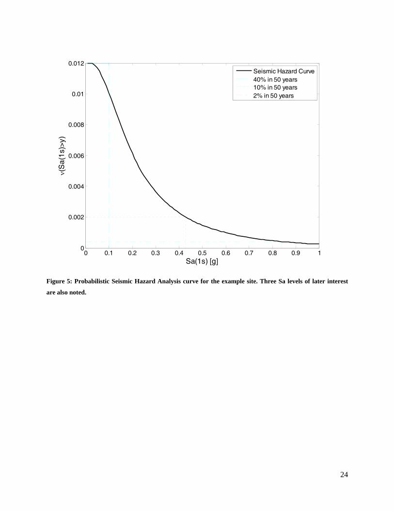
The ground motion hazard curve obtained from this calculation for this simplified site is
shown in Figure 5. This calculation is comparable to that used to produce the hazard curves
available on the USGS website (http://earthquake.usgs.gov/research/hazmaps/), for real sites in
the United States. Two typical design levels (2% and 10% in 50 years) along with an additional
illustrative design level (40% in 50 years) are marked in Figure 5. Using a Poisson model for
earthquake recurrence, a Sa exceedance probability of 2% in 50 year is equivalent to ν(Sa > y) =
0.0004 (a return period of 2475 years), and hence a target Sa value, Sa(1s)* of 0.84g. Similarly,
Sa exceedance probabilities of 10% and 40% in 50 years are equivalent to return periods of 475
and 100 years, and have target Sa(1s)* values of 0.43g and 0.10g, respectively. The following
plots of disaggregation results and CMS calculations have these three design levels Sa levels
marked for reference.
4.2 Disaggregation of Events
The conditional probability that each event caused Sa > y is given by Equation (15).
)(),()|(
ySavEventySaySaEventP i
i >>
=>ν (15)
where

13
∑ >=>j
ijiji EventGMPMPEventGMPMySaPEventySa )()(),|(),( νν (16)
The probabilities obtained from Equation (15) are plotted in Figure 6. From Figure 6, we
can see that the smaller but more frequent Event A is most likely to cause exceedance of small
Sa amplitudes, whereas Event B is most likely to cause exceedance of large Sa amplitudes. This
is because the annual hazard rate involves two competing factors: annual rate of occurrence for
an earthquake, and probability of exceeding a Sa level given that earthquake. Small earthquakes
(for example, Event A) have a larger annual rate of occurrence than large earthquakes, whereas
large earthquakes (for example, Event B) have a larger probability of exceeding a Sa level. At a
lower Sa level, the hazard is dominated by small frequent earthquakes; at a higher Sa level, the
hazard is dominated by large but infrequent earthquakes because the small earthquakes very
rarely generate such large ground motion amplitudes. The results in Figure 6 are typical of PSHA
analyses for more realistic sites.
4.3 Disaggregation of Ground Motion Prediction Models
Following Equation (8), the disaggregation of GMPMs is performed using the following
equations,
)(),(
)|(ySav
GMPMySaySaGMPMP j
j >>
=>ν
(17)
where
∑ >=>i
ijijj EventGMPMPEventGMPMySaPGMPMySa )()(),|(),( νν (18)
Note the similarity between Equations (16) and (18). The results of this disaggregation
calculation are shown in Figure 7. The disaggregated GMPM contributions vary from 0.16 to
0.31, instead of having an equal weight of 0.25. The weights are still not too far from 0.25.
GMPM disaggregation is useful for computation of CMS, as the disaggregated probabilities of
GMPMs offer additional insights into which GMPM contributes most to the prediction of Sa
values of interest.
4.4 Disaggregation of Magnitude, Distance, and Epsilon
Since only one magnitude is associated with each event, the disaggregated mean
magnitude can be found easily by determining the sum of the products of the magnitudes given
an event and the disaggregated contribution of the event, as follows:

14
∑ >=>i
ii ySaEventPEventMySaM )|()|(|_
(19)
where M is used to denote the mean value of M . Note that in this example iEventM | is a
deterministic relationship, since there is only a single magnitude associated with each event.
This equation is equivalent to Equation (5).
The disaggregated mean magnitude can be found using a similar method separately, for
each GMPM, as shown in Equation (20). The results are shown in Figure 8. In this figure, the
thin lines indicate the mean magnitude, given Sa > y and given that the associated GMPM was
the model that predicted Sa > y, ySaGMPMM j >,|_
. The heavy line provides the a weighted
average (composite) of ySaGMPMM j >,|_
over all GMPMs. The variation of disaggregated
mean magnitudes, is greater at higher Sa values because that is where the GMPMs differ more
significantly due to lack of data to constrain the predictions.
∑ >=>=>i
jijijj ySaGMPMEventPGMPMEventMySaGMPMMySaM ),|(),|(,||__
(20)
Since only one distance is associated with each event, the disaggregated mean distance
can be found easily by determining the sum of the products of the distance given an event and
the disaggregated contribution of the event, as follows:
∑ >=>i
ii ySaEventPEventRySaR )|()|(|_
(21)
The disaggregated mean distance values are plotted in Figure 9. In this case the results
are very similar to the magnitude disaggregation results due to the one-to-one correspondence
between magnitudes and distances in this simple example.
For each event (M = m, R = r), epsilon values change as Sa varies. The centroidal values
of epsilon given Sa > y and an event, iEventySa ,|_
>ε can be obtained from Equation (5). The
disaggregated mean epsilon can be computed as follows:

15
∑ >>=>i
ii ySaEventPEventySaySa )|(),|(|__εε (22)
The disaggregated mean epsilon values are plotted in Figure 10. As Sa increases, the
mean ε value increases, and this can have a large impact on the shape of the CMS that will be
computed in the next section.
4.5 Conditional Mean Spectrum Computation Using Two Approaches
With the disaggregation information of the previous few sections, it is now possible to
compute the CMS using Equation (11). The first-mode period of interest in this example is 1s
and our first example calculation is conditioned on Sa exceeding 0.84g, we use the disaggregated
mean values of M, R, and ε given Sa(1s) > 0.84g. The mean predictions of lnSa at other periods,
using each GMPM, are then computed using Equation (11).
There are two approaches to CMS computation using multiple GMPMs.
For Approach 1, we first compute the mean M, R, and ε given Sa > y using all GMPMs,
from Equations (19), (21), and (22).
Then we compute CMSj, the CMS computed using GMPMj and the mean M, R, and
ε given all GMPMs, from Equations (19), (21), and (22) as follows:
)|,|,|(___
ySaySaRySaMCMSCMS jj >>>= ε (23)
The result from equation (23) on its own is also the “Approach 0” mentioned above, as it
can be used on its own as a simple way to obtain a CMS.
To use the results of equation (23) in Approach 1, we compute a weighted sum of these
CMSj, using the assigned weight of GMPM (0.25 in this case), as follows:
∑∑ ==j
jj
jj CMSGMPMPCMSCMS )25.0()( (24)
The results from equations (23) and (24) are shown in Figure 11. The result from
equation 24 is denoted “CMS, Composite” as it is a composite of the individual CMS spectra
from equation (23).
Similarly for Approach 2, first we compute the mean given Sa > y using each GMPM.
Note that the disaggregation means used here here are conditional on each GMPM (e.g., using ,
Equation (20)), instead of on all GMPMs, as in Approach 1.

16
Then we compute CMSj’, the CMS computed using GMPMj and the respective mean M,
R, and ε given each GMPM, from procedures similar to Equation (20).
)|,|,|('___
ySaySaRySaMCMSCMS jjjjj >>>= ε (25)
Equation (25) is identical to Equation (23), except that the GMPM-specific M/R/ε values of
Equation (25) are used in place of the overall M/R/ε disaggregation values.
Finally for Approach 2, we compute a weighted sum of these CMSj’ (composite curve in
Figure 12), using the disaggregated contribution of GMPMs. Note that probability of GMPM
here is conditional on Sa > y, and it differs from the assigned equal probability. This
disaggregated probability of GMPM adds insights regarding the relative contribution of GMPM
to the prediction of the Sa level of interest. The extension of PSHA disaggregation to GMPMs
offers a more complete solution compared to the original approach.
∑ >=j
jj ySaGMPMPCMSCMS )|('' (26)
Figure 13 shows that the approaches of Equations (24) and (26) are not equivalent.
Approach 0 is a raw attempt to compute the CMS using a single GMPM with available data.
Approach 1 is a simplified method to obtain a composite CMS by averaging the conditional
mean spectra obtained from each of the GMPMs. Approach 2 computes a weighted average of
the GMPM-specific conditional mean spectra, where the weights come from GMPM
disaggregation, and is thus probabilistically consistent. The drawback for Approach 2 is that we
need additional data (i.e., the disaggregation of GMPMs and the disaggregation of magnitude,
distance, and epsilon for each GMPM) which are not readily available from current PSHA
calculation tools or the USGS website. There is a large scatter among different single-GMPM
CMSs in Approach 0, showing the variability among different GMPMs. However, the difference
between Approach 1 and Approach 2 is not significant in this example, which suggests that we
may be able to approximate Approach 2 using the simpler Approach 1. Further calculations in
more varied and more realistic conditions are needed to confirm this possibility.
To investigate the effect of change in design level and period of interest on the accuracy
of these approaches, four combinations with three design levels and two periods of interest are
shown: a) Sa(1s) > 0.84g, corresponding to 2% in 50 years Sa exceedance (Figure 13); b) Sa(1s)
> 0.43g, corresponding to 10% in 50 years Sa exceedance (Figure 14); c) Sa(1s) > 0.10g,

17
corresponding to 40% in 50 years Sa exceedance (Figure 15); d) Sa(0.2s) > 0.84g, corresponding
to 10% in 50 years Sa exceedance but at a different period of interest (Figure 16).
An examination of Equation (11) reveals the components of CMS computation at various
design levels, i.e. target Sa(T1)*. As the target Sa(T1)* value changes, the disaggregated mean
M/R/ε change, which change Sa prediction in terms of μlnSa and σlnSa. The correlation coefficient
ρ, on the other hand, is not dependent on the target Sa(T1)* value. As ε increases, ερ increases,
resulting in a larger difference between Sa at the period of interest (usually the first-mode period)
and Sa at periods further away from the period of interest and hence a sharper spectral shape.
This is apparent in Figure 17: the three CMSs using the same approach differ as a result of the
variation in the mean disaggregated epsilon values as shown in Figure 10. For instance, a
decrease in target Sa from 0.84g to 0.43g results in a decrease in ε from 1.90 to 1.22 (as well as
a decrease of M from 7.48 to 7.12 and a decrease of R from 21.1 to 18.4), which results in a
flatter CMS given Sa(1s) > 0.43g.
To evaluate the appropriateness of approximating Approach 2 using Approach 1 at a
single Sa(T1)*, we can look at both the disaggregated mean M/R/ε and disaggregated GMPM
contribution. If the disaggregated mean M/R/ε is similar for different GMPMs (e.g.,
ySaMySaM j >≈> ||__
) at Sa(T1)*, μlnSa and σlnSa will be similar, i.e. CMSj’ (Equation (25)) is
similar to CMSj (Equation (23)). Approach 1 (Equation (24)) and Approach 2 (Equation (26))
are weighted averages of CMSj / CMSj’ respectively and thus will give similar results of
CMS/CMS’. In other words, the relative contribution of GMPMs in Equation (26) does not
matter much since CMSj’ is almost equal to CMSj.
On the other hand, if the disaggregated mean M/R/ε vary a great deal for various
GMPMs, the GMPM specific CMSj’ will be substantially different from the general CMSj. The
relative contribution of GMPMs then accounts for the difference in CMS and CMS’. However, if
the relative contribution of GMPMs is about equal, then the average CMS’ is similar to CMS,
despite the difference between CMSj’ and CMSj. The difference between CMS’and CMS for
Sa(1s) > 0.10g (Figure 15) is much smaller than that for Sa(1s) > 0.84g (Figure 13), because the
disaggregated mean M/R/ε differ less among different GMPMs for Sa(1s) > 0.10g (from Figure 7
to Figure 9), resulting in a smaller difference between CMSj’ and CMSj, and a less important
relative contribution of GMPMs which is also closer to the equal value (0.25 in this example).

18
CMSj employs the same overall disaggregated mean M/R/ε (e.g., ySaM >|_
) whereas
CMSj’utilizes GMPM-specific disaggregated mean M/R/ε (e.g.,
ySaM j >|_
). Since the same
M/R/ε are used for CMSj, the scatter in CMSj in Approach 0 (Figure 11) reflects the variability in
Sa prediction by different GMPMs. However, CMSj’ (Figure 12) shows a larger scatter than
CMSj (Figure 11), with variability from both Sa prediction and disaggregation of M/R/ε. If the
disaggregation of M/R/ε differ very little among different GMPMs, there will be a smaller
difference between CMSj’ and CMSj.
When the design level or period of interest changes, the event that causes Sa(T1) >
Sa(T1)* (shown by disaggregated mean M/R/ε ) varies. With the same period of interest, when
the design level changes, the spectral shape changes, as shown in Figure 17. With the same
design level, when the period of interest changes, the spectral shape changes, as shown in Figure
18. The former can be used to select ground motions for the same structure at various design
levels, potentially used in incremental dynamic analysis. The latter can be used to select ground
motions for different structures at the same design level, or alternatively, select ground motions
for the same structure with various periods of interest (e.g. first-mode period and higher mode
period for a tall building) at the same design level, potentially using multiple CMSs (Baker
2005).
5 Discussion and Conclusions
The application of conditional mean spectrum (CMS) computation to multiple ground
motion prediction models (GMPMs) requires the disaggregation of GMPMs. This approach is
consistent with the probabilistic treatment of random variables in traditional probabilistic seismic
hazard analysis (PSHA), and is an extension from the currently available method of
disaggregation of events. The CMS method applied directly to the disaggregated mean M, R,
and ε considering all GMPMs, may produce different results from that applied to the
disaggregated mean M, R, and ε considering each GMPM separately, along with its associated
disaggregated contribution. The spectral shape of CMS, as well as the causal event, varies as the
design level or the period of interest changes. CMS using multiple GMPMs has practical
significance since multiple GMPMs are usually used to obtain an aggregate hazard rate. It will
be probabilistically consistent to consider the conditional relative contribution of GMPMs. The

19
disaggregation of GMPMs provides additional insights into which GMPM contributes most to
prediction of Sa values of engineering interest.
Currently, GMPM disaggregation is typically not available (e.g., from USGS hazard
maps). CMS applied directly to the disaggregated mean M, R, and ε considering all GMPMs
without the disaggregation of GMPMs and the disaggregation of M, R, and ε with respect to each
GMPM, may produce inaccurate results, especially for cases where disaggregation of M, R, and ε
differ significantly using different GMPMs. Although the computation of CMS using multiple
GMPM is slightly more complicated, the improved accuracy may be worthwhile in some cases.
Performing GMPM disaggregation in typical PSHA calculations would be very beneficial
in facilitating the improved CMS calculations presented in this paper. We can further extend
disaggregation to other ground motion parameters, such as earthquake fault types, to more
accurately represent the parameters that contribute most to Sa values of engineering interest.
Future collaborations with USGS are essential to overcome challenges in practical
implementation of CMS using multiple GMPMs. Such implementation can be incorporated into
future USGS hazard maps and made available to the public, which would then facilitate the CMS
calculation procedure above and aid ground motion selection efforts.
Acknowledgments
This work was supported by the U.S. Geological Survey, under Award Number
07HQAG0129. Guidance, assistance, and timely feedback provided by the P.I., Dr. Jack Baker,
are gratefully appreciated and acknowledged here. Any opinions, findings, and conclusions or
recommendations presented in this material are those of the author and do not necessarily reflect
those of the funding agency.

20
Figure 1: Probability density function of epsilons demonstrating the difference between McGuire disaggregation (ε∗) and Bazzurro and Cornell disaggregation ( ε ).
00
1
PDF of εPDF of ε, given Sa>y
*ε ε ε
fΕ(ε)

Figure 2: L
Layout of an eexample site d
dominated by
two earthquaake events A and B.
21

22
Abrahamson and Silva p = 0.25 Event A Boore et al. p = 0.25
νA Campbell p = 0.25 Sadigh et al. p = 0.25
Abrahamson and Silva p = 0.25 Event B Boore et al. p = 0.25
νB Campbell p = 0.25 Sadigh et al. p = 0.25
Figure 3: Logic tree of GMPMs used to calculate hazard in the example site.

23
Figure 4: Prediction of ground motion exceedance for two events using four different GMPMs in the example
site.
0 0.1 0.2 0.3 0.4 0.5 0.6 0.7 0.8 0.9 10
0.1
0.2
0.3
0.4
0.5
0.6
0.7
0.8
0.9
1
Sa(1s) [g]
P(S
a(1
s)>
y|E
ven
t i, GM
PM
j)
Event A, Abrahamson and SilvaEvent A, Boore et al.Event A, CampbellEvent A, Sadigh et al.Event B, Abrahamson and SilvaEvent B, Boore et al.Event B, CampbellEvent B, Sadigh et al.
24
Figure 5: Probabilistic Seismic Hazard Analysis curve for the example site. Three Sa levels of later interest
are also noted.
0 0.1 0.2 0.3 0.4 0.5 0.6 0.7 0.8 0.9 10
0.002
0.004
0.006
0.008
0.01
0.012
Sa(1s) [g]
ν(S
a(1
s)>
y)
Seismic Hazard Curve40% in 50 years10% in 50 years2% in 50 years

25
Figure 6: Disaggregation of events, given Sa(1s) > y, for the example site. Disaggregation results
corresponding to Sa exceedance probabilities of 40%, 10%, and 2% in 50 years are marked on the figure.
0 0.1 0.2 0.3 0.4 0.5 0.6 0.7 0.8 0.9 10
0.1
0.2
0.3
0.4
0.5
0.6
0.7
0.8
0.9
1
Sa(1s) [g]
P(E
ven
t i|Sa
(1s)
>y)
Event AEvent B40% in 50 years10% in 50 years2% in 50 years

26
Figure 7: Disaggregation of GMPMs, given Sa(1s) > y, for the example site.
0 0.1 0.2 0.3 0.4 0.5 0.6 0.7 0.8 0.9 10.16
0.18
0.2
0.22
0.24
0.26
0.28
0.3
0.32
Sa(1s) [g]
P(G
MP
Mj|S
a(1
s)>y
)
Abrahamson and SilvaBoore et al.CampbellSadigh et al.40% in 50 years10% in 50 years2% in 50 years

27
Figure 8: Disaggregation of magnitude M, given Sa(1s) > y, for the example site.
0 0.1 0.2 0.3 0.4 0.5 0.6 0.7 0.8 0.9 16.2
6.4
6.6
6.8
7
7.2
7.4
7.6
7.8
8
Sa(1s) [g]
E(M
|Sa(
1s)
>y)
CompositeAbrahamson and SilvaBoore et al.CampbellSadigh et al.40% in 50 years10% in 50 years2% in 50 years

28
Figure 9: Disaggregation of distance R, given Sa(1s) > y, for the example site.
0 0.1 0.2 0.3 0.4 0.5 0.6 0.7 0.8 0.9 112
14
16
18
20
22
24
26
Sa(1s) [g]
E(R
|Sa
(1s)
>y)
CompositeAbrahamson and SilvaBoore et al.CampbellSadigh et al.40% in 50 years10% in 50 years2% in 50 years

29
Figure 10: Disaggregation of epsilon ε, for the example site.
0 0.1 0.2 0.3 0.4 0.5 0.6 0.7 0.8 0.9 10
0.5
1
1.5
2
2.5
Sa(1s) [g]
E( ε
|Sa
(1s)
>y)
CompositeAbrahamson and SilvaBoore et al.CampbellSadigh et al.40% in 50 years10% in 50 years2% in 50 years

30
Figure 11: CMS computation using Approach 1 conditional on Sa(T1 = 1s) > 0.84g (2% in 50 years), for the
example site.
10-1
100
10-1
100
T [s]
Sa
(T) [
g]
CMS, CompositeCMS, Abrahamson and SilvaCMS, Boore et al.CMS, CampbellCMS, Sadigh et al.Target Sa(T
1)*

31
Figure 12: CMS computation using Approach 2 conditional on Sa(T1 = 1s) > 0.84g (2% in 50 years), for the
example site.
10-1
100
10-1
100
T [s]
Sa
(T) [
g]
CMS, CompositeCMS, Abrahamson and SilvaCMS, Boore et al.CMS, CampbellCMS, Sadigh et al.Target Sa(T
1)*

32
Figure 13: Comparison of CMS computation using Approaches 0, 1, and 2 conditional on Sa(T1 = 1s) > 0.84g
(2% in 50 years), for the example site.
10-1
100
10-1
100
T [s]
Sa
(T) [
g]
CMS, Approach 0, Abrahamson and SilvaCMS, Approach 0, Boore et al.CMS, Approach 0, CampbellCMS, Approach 0, Sadigh et al.CMS, Approach 1CMS, Approach 2Target Sa(T
1)*

33
Figure 14: Comparison of CMS computation using Approaches 0, 1, and 2 conditional on Sa(T1 = 1s) > 0.43g (10% in 50 years), for the example site.
10-1
100
10-1
100
T [s]
Sa
(T) [
g]
CMS, Approach 0, Abrahamson and SilvaCMS, Approach 0, Boore et al.CMS, Approach 0, CampbellCMS, Approach 0, Sadigh et al.CMS, Approach 1CMS, Approach 2Target Sa(T
1)*

34
Figure 15: Comparison of CMS computation using Approaches 0, 1, and 2 conditional on Sa(T1 = 1s) > 0.10g (40% in 50 years), for the example site.
10-1
100
10-1
100
T [s]
Sa
(T) [
g]
CMS, Approach 0, Abrahamson and SilvaCMS, Approach 0, Boore et al.CMS, Approach 0, CampbellCMS, Approach 0, Sadigh et al.CMS, Approach 1CMS, Approach 2Target Sa(T
1)*

35
Figure 16: Comparison of CMS computation using Approaches 0, 1, and 2 conditional on Sa(T1 = 0.2s) >
0.84g (10% in 50 years).
10-1
100
10-1
100
T [s]
Sa
(T) [
g]
CMS, Approach 0, Abrahamson and SilvaCMS, Approach 0, Boore et al.CMS, Approach 0, CampbellCMS, Approach 0, Sadigh et al.CMS, Approach 1CMS, Approach 2Target Sa(T
1)*

36
Figure 17: CMS conditional on Sa(1s) > Sa(T1)* for 2% in 50 years (Sa(T1)* = 0.84g), 10% in 50 years (Sa(T1)* = 0.43g), and 40% in 50 years (Sa(T1)* = 0.10g) design levels.
10-1
100
10-1
100
T [s]
Sa
(T) [
g]
CMS, Approach 1, Sa(1s) > 0.84gCMS, Approach 2, Sa(1s) > 0.84gTarget Sa(T
1)*, Sa(1s) > 0.84g
CMS, Approach 1, Sa(1s) > 0.43gCMS, Approach 2, Sa(1s) > 0.43gTarget Sa(T
1)*, Sa(1s) > 0.43g
CMS, Approach 1, Sa(1s) > 0.10gCMS, Approach 2, Sa(1s) > 0.10gTarget Sa(T
1)*, Sa(1s) > 0.10g

37
Figure 18: CMS conditional on Sa(T1) > Sa(T1)* for 10% in 50 years design level (Sa(1s)* = 0.43g and Sa(0.2s)* = 0.84g).
10-1
100
10-1
100
T [s]
Sa
(T) [
g]
CMS, Approach 1, Sa(1s) > 0.43gCMS, Approach 2, Sa(1s) > 0.43gTarget Sa(T
1)*, Sa(1s) > 0.43g
CMS, Approach 1, Sa(0.2s) > 0.84gCMS, Approach 2, Sa(0.2s) > 0.84gTarget Sa(T
1)*, Sa(0.2s) > 0.84g

38
6 References: Abrahamson, N. A., and Silva, W. J. (1997). "Empirical response spectral attenuation relations
for shallow crustal earthquakes." Seismological Research Letters, 68(1), 94-127. Baker, J. W. (2005). "Vector-valued ground motion intensity measures for probabilistic seismic
demand analysis," Thesis (Ph D ), Stanford University, 2005. Baker, J. W., and Cornell, C. A. (2006). "Spectral shape, epsilon and record selection."
Earthquake Engineering & Structural Dynamics, 35(9), 1077-1095. Baker, J. W., and Jayaram, N. (2008). "Correlation of spectral acceleration values from NGA
ground motion models." Earthquake Spectra, 24(1), 299-317. Bazzurro, P., and Cornell, C. A. (1999). "Disaggregation of seismic hazard." Bulletin of the
Seismological Society of America, 89(2), 501-520. Boore, D. M., Joyner, W. B., and Fumal, T. E. (1997). "Equations for estimating horizontal
response spectra and peak acceleration from western North American earthquakes: a summary of recent work." Seismological Research Letters, 68(1), 128-153.
Campbell, K. W. (1997). "Empirical near-source attenuation relationships for horizontal and vertical components of peak ground acceleration, peak ground velocity, and pseudo-absolute acceleration response spectra." Seismological Research Letters, 68(1), 154-179.
Frankel, A. D., Petersen, M. D., and Mueller, C. S. (2002). "Documentation for the 2002 Update of the National Seismic Hazard Maps." USGS, Denver, Colorado.
Kramer, S. L. (1996). Geotechnical earthquake engineering, Prentice Hall, Upper Saddle River, N.J.
McGuire, R. K. (1995). "Probabilistic seismic hazard analysis and design earthquakes; closing the loop." Bulletin of the Seismological Society of America, 85(5), 1275-1284.
Sadigh, K., Chang, C. Y., Egan, J. A., Makdisi, F., and Youngs, R. R. (1997). "Attenuation relationships for shallow crustal earthquakes based on California strong motion data." Seismological Research Letters, 68(1), 180-189.
Scherbaum, F., Schmedes, J., and Cotton, F. (2004). "On the Conversion of Source-to-Site Distance Measures for Extended Earthquake Source Models." Bulletin of the Seismological Society of America, 94(3), 1053-1069.
Strasser, F. O., Bommer, J. J., and Abrahamson, N. A. (2008). "Truncation of the distribution of ground-motion residuals." J. Seismol(12), 79-105.