baker kelly thesis - texas tech university
TRANSCRIPT

Local and Landscape Factors Influencing
Diversity and Fitness in Odonates at Playa Wetlands
by
Kelly S. Baker, B.S.
A Thesis
in
Biology
Submitted to the Graduate Faculty
of Texas Tech University in
Partial Fulfillment of
the Requirements for
the Degree of
MASTER OF SCIENCE
Approved
Dr. Nancy E. McIntyre
Chair of Committee
Dr. Kevin Mulligan
Dr. Richard E. Strauss
Peggy Gordon Miller
Dean of the Graduate School
August, 2011

Copyright 2011, Kelly Baker

Texas Tech University, Kelly Baker, August 2011
ii
ACK�OWLEDGME�TS
The completion of this work would not have been possible without the help and
support of many different people.
First and foremost, I would like to thank my committee chair Dr. Nancy
McIntyre. In addition to providing lab space and resources, Dr. McIntyre has generously
given advice and direction from the inception of this project to its close. It has been a
blessing to work under the counsel of such a kind and scholarly advisor. I would also
like to thank my other committee members, Dr. Richard Strauss and Dr. Kevin Mulligan,
both of whose advice and help has been invaluable. Dr. Strauss was chiefly responsible
for the statistical component of chapter II; without his input, this project would not have
been a success. Similarly, I am indebted to Dr. Mulligan for his ArcGIS expertise, as his
help was also instrumental in the completion of chapter II. Furthermore, I would like to
acknowledge Dr. Bryan Reece for his assistance in developing the oviposition chambers,
as well as his significant role in data collection for the biodiversity chapter. I would like
to thank Chris Van Nice for his ArcGIS guidance and Steve Collins for his input
throughout all stages of this project.
Over the course of the last several years, I have received funding from three
different organizations. I would like to extend the sincerest of thanks to AT&T for
providing the AT&T Chancellor’s Fellowship, Texas Tech Graduate School and Sandy
Land Underground Water Conservation District for providing the Water Conservation
Research Fellowship, and lastly, the Department of Biological Sciences at Texas Tech
University for its constant and faithful financial investment in its graduate students.

Texas Tech University, Kelly Baker, August 2011
iii
Through the efforts of Dr. John Zak and Dr. Llewellyn Densmore (as well as countless
others), the biology graduate students have been blessed with liberal TA and RA funding.
On a personal note, I would like to thank my loving husband Joshua who
provided not only an abundance of moral support, but also field and lab assistance when
necessary. Also, I am deeply appreciative of my parents, Mark and Brenda Klinkerman,
who have always been a source of strength and encouragement. Finally, I would like to
thank God, the loving Creator, in whom I find joy and hope.

Texas Tech University, Kelly Baker, August 2011
TABLE OF CO�TE�TS
ACK�OWLEDGME�TS ii
LIST OF TABLES vi
LIST OF FIGURES vii
CHAPTER
I. I�TRODUCTIO� 1
Literature Cited 5
II. LOCAL A�D LA�DSCAPE-LEVEL VARIABLES IMPORTA�T
I� THE DETERMI�ATIO� OF ODO�ATE OCCURRE�CE A�D
RICH�ESS 7
Abstract 7
Introduction 8
Methods 10
Results 16
Discussion 21
Literature Cited 27
Tables and Figures 30
III. ASSOCIATIO�S BETWEE� ADULT FEMALE BODY SIZE
A�D FIT�ESS I� ODO�ATES 67
Abstract 67
Introduction 68
Methods 69
Results 74

Texas Tech University, Kelly Baker, August 2011
Discussion 76
Literature Cited 84
Tables and Figures 88

Texas Tech University, Kelly Baker, August 2011
vi
LIST OF TABLES
2.1. Correct classification table for landscape-level multiple logistic regression 30
2.2. Correct classification table for local-level multiple logistic regression 31
2.3. Correct classification table for landscape-level PLS discriminant analysis 32
2.4. Correct classification table for local-level PLS discriminant analysis 33
2.5. Landscape-level variables by number 34
2.6. Local-level variables by number 35
2.7. Landscape-level multiple logistic regression coefficients 36
2.8. Local-level multiple logistic regression coefficients 43
2.9. Landscape-level PLS discriminant analysis coefficients 45
2.10. Local-level PLS discriminant analysis coefficients 52
2.11. Landscape-level PLS multiple regression coefficients 54
2.12. Local-level multiple logistic regression coefficients 55
3.1. Results of t-tests for fitness relationships in female E. civile 88
3.2. Correlation results related to overall E. civile fitness 89
3.3. Post-hoc Tukey test results for the relationship between HCW of females
caught early in the season (June 23-July 6) and females caught late in the
season (September 2-8) 90
3.4. Data for egg-laying female E. civile for 2009 and 2010 91
3.5. Egg-length data for female E. civile clutches in 2010 98
3.6. Data for non-egg-laying female E. civile for 2009 and 2010 102

Texas Tech University, Kelly Baker, August 2011
vii
LIST OF FIGURES
2.1. Distribution of actual species richness (a) and log richness (b) 56
2.2. Landscape-level multiple logistic regression results by species 57
2.3. Local-level multiple logistic regression results by species 59
2.4. Landscape-level PLS discriminant analysis results by species 61
2.5. Local-level PLS discriminant analysis results by species 63
2.6. Landscape-level PLS multiple regression variable weights 65
2.7. Local-level PLS multiple regression variable weights 66
3.1. Distribution of clutch size 108
3.2. Distribution of time to hatch 109
3.3. Distribution of hatch duration 110
3.4. Distribution of hatch success 111
3.5. Distribution of mean egg length 112
3.6. HCW of egg-laying vs. non-egg-laying females 113
3.7. Pearson correlation of HCW and mean egg length 114
3.8. Pearson correlation of HCW and hatch success 115
3.9. Pearson correlation of HCW and hatch duration 116
3.10. Pearson correlation for number of eggs and mean egg length 117
3.11. Spearman correlation of hatch duration and mean egg length 118
3.12. Pearson correlation of number of eggs and hatch success 119
3.13. Pearson correlation of mean egg length and hatch success 120
3.14. Pearson correlation of hatch duration and hatch success 121

Texas Tech University, Kelly Baker, August 2011
1
CHAPTER I
I�TRODUCTIO�
Anthropogenic changes to the environment are inevitable and continual,
especially with the increasing human population. Building homes, growing crops, raising
livestock, and the pursuit of hobbies all come with environmental costs. This can be seen
acutely in the landscape of the southernmost portion of the Great Plains of North
America, the Southern High Plains.
In the most simplistic terms, the ecosystem of the Southern High Plains is
cropland and grassland. In Texas, this region is highly agricultural: around 46% of the
Southern High Plains is composed of cropland (chiefly cotton, corn, sorghum, and winter
wheat), with agriculture being the primary economic driver of the region (Haukos and
Smith 1994, Smith 2003). Grasslands in the Southern High Plains comprise indigenous
grasslands and Conservation Reserve Program (CRP) grasslands (former cropland
restored to grassland). Indigenous grasslands account for approximately 37% of the
Southern High Plains whereas CRP makes up about 12% (Haukos and Smith 1994). The
main source of above-ground freshwater is playa wetlands, comprising approximately 2%
of the landscape.
Playas are shallow, ephemeral ponds with highly variable hydroperiods.
Typically, playas are less than 1.5 meters in depth (Smith 2003: 9) with an average
surface area of 6.3 hectares (ranging from less than one hectare to more than 260
hectares) (Guthery and Bryant 1982). Playa hydroperiods are defined by alternating
intervals of wet and dry, but no specification exists as to the lengths of these intervals.
Some playas will fill and dry several times in one year whereas others may go several

Texas Tech University, Kelly Baker, August 2011
2
years before either filling or drying out (Smith 2003: 8-9). The soils in a playa wetland
are distinct from those of the surrounding Great Plains uplands (Mulligan and Fish 2004),
in that they are hydric soils with high clay content. When wet, the hydric soil expands
and helps retain water in the wetland basin. There are approximately 30,000 playas in the
Great Plains (Osterkamp and Wood 1987). However, the exact number of the playa lakes
on the Southern High Plains is difficult to discern because of the varying hydroperiod of
playas, road construction through these wetlands, and their continuing loss to agricultural
pursuits.
Playas have significant ecological and economic value. Ecologically, these
wetlands are a focal point for regional biodiversity (Haukos and Smith 1994).
Economically, playas provide water to support human life through direct consumption
and especially irrigation-based agriculture relying upon the Ogallala Aquifer, as playas
are the primary method of Ogallala recharge (Playa Lakes Joint Venture website,
accessed 23 October 2008:
http://www.pljv.org/assets/Media/News%20Release_Playas%20Recharge%20Ogallala_0
70927.pdf).
While anthropogenic environmental change is a well-established issue, scientists
are continually discovering new and different ways in which human activity effects
ecosystems. Several recent studies have emerged revealing that playas are affected by
the varying land cover forms within their watersheds. Sedimentation occurs at a much
higher rate in cropland watersheds than in grassland playas (Luo et al. 1997, Tsai et al.
2007). Sedimentation alters the hydroperiod of a playa by increasing evaporation and
infiltration (by pushing water beyond the boundary of the clay hydric soil). Additionally,

Texas Tech University, Kelly Baker, August 2011
3
cropland ecosystems are often more heterogeneous than are grassland ecosystems,
increasing the difficulty of dispersal for terrestrial organisms (Gray et al. 2004). Finally,
because of the fertilizers, herbicides, and pesticides used on agricultural fields, the water
chemistry of cropland playas is altered relative to that of grassland playas.
Because of the biological and economical worth of playas to the Southern High
Plains region, it is timely to invest in research aimed at understanding and preserving the
well-being of these wetlands. From a broad perspective, the objectives of my thesis were
to examine how anthropogenic environmental changes have impacted odonates
(dragonflies and damselflies), a local amphibious invertebrate group championed as an
indicator taxon for playa health (Hernandez et al. 2006).
My second chapter explores the factors governing odonate biodiversity at playa
wetlands. As discussed above, the literature confirms that interactions occur between a
playa and the upland ecosystem. Therefore, an aquatic or amphibious organism
inhabiting a playa (such as odonates) must deal not only with immediate variables (such
as water temperature, hydroperiod, depth, etc.) but also with larger-scaled factors (such as
land use/land cover) that may have both direct influences and indirectly act through
proximal variables. Up to this point, the extent to which these interactions affect aquatic
or amphibious organisms has been drastically understudied. In this chapter, I sought to
determine which factors (from suites of local and landscape-level variables) most
influence the occurrence of odonates at playa wetlands on the Southern High Plains.
My third chapter builds on the work of Dr. Bryan Reece. In lab experiments,
Reece found that odonate larval growth and development are influenced by different
environmental variables, such as pH and temperature, which are essentially determined

Texas Tech University, Kelly Baker, August 2011
4
by the playa’s surrounding ecosystem. For example, pH is determined by chemical
inputs from the surrounding ecosystem, whereas temperature is dependent upon playa
depth, which is affected by sedimentation (which itself is ultimately affected by
surrounding land use). These factors affect odonate growth and development by
influencing the rate at which they occur. Odonates have the ability to sense habitat
quality as they mature. If the habitat quality is poor, the larvae may grow and develop
faster in order to escape adverse conditions. The assumption is that faster growth and
development cause a tradeoff of smaller adult body size (De Block and Stoks 2005,
Mikolajewski et al. 2005). Therefore, researching the relationship between adult female
body size and fitness is the next logical step in exploring the mechanistic effects of
environmental variables on these organisms.
The two separate studies of my thesis are linked conceptually in examining how
aspects of the environment affect the distribution and life history of organisms. The
second chapter utilizes a GIS approach to analyze a long-term dataset on odonate
diversity. The third chapter explains a lab-based study on one focal odonate species.
Together, they provide more information on how the ecology of playa organisms is
influenced by anthropogenic modifications to the Southern High Plains landscape.

Texas Tech University, Kelly Baker, August 2011
5
Literature Cited
De Block, M., and R. Stoks. 2005. Fitness effects from egg to reproduction: Bridging
the life history transition. Ecology 86:185-197.
Gray, M.J., L.M. Smith, and R.I. Leyva. 2004. Influence of agricultural landscape
structure on a Southern High Plains, USA, amphibian assemblage. Landscape
Ecology 19:719-729.
Guthery, F.S., and F.C. Bryant. 1982. Status of playas in the Southern Great Plains.
Wildlife Society Bulletin 10:309-317.
Haukos, D.A., and L.M. Smith. 1994. The importance of playa wetlands to biodiversity
of the Southern High Plains. Landscape and Urban Planning 28:83-98.
Hernandez, K.M., B.A. Reece, and N.E. McIntyre. 2006. Effects of anthropogenic land
use on Odonata in playas of the Southern High Plains. Western North American
Naturalist 66:273-278.
Luo, H.R., L.M. Smith, B.L. Allen, and D.A. Haukos. 1997. Effects of sedimentation on
playa wetland volume. Ecological Applications 7:247–52.
Mikolajewski, D.J., Brodin, T., Johansson, F., and G. Joop. 2005. Phenotypic plasticity
in gender specific life-history: effects of food availability and predation. Oikos
110: 91-100.
Mulligan, K.R., and E.B. Fish. 2004. Mapping Playa Lake Basins on the Llano Estacado,
Texas, GIS. The Language of Geography, ESRI Map Book, vol. 19.

Texas Tech University, Kelly Baker, August 2011
6
Osterkamp, W.R., and W.W. Wood. 1987. Playa-lake basins on the Southern High
Plains of Texas and New Mexico; Part I, Hydrologic, geomorphic, and geologic
evidence for their development. Geological Society of America Bulletin 99:215-
233.
Smith, L.M. 2003. Playas of the Great Plains. University of Texas Press, Austin, TX.
Tsai, J.-S., L.S. Venne, S.T. McMurry, and L.M. Smith. 2007. Influences of land use
and wetland characteristics on water loss rates and hydroperiods of playas in the
Southern High Plains, USA. Wetlands 27:683-692.

Texas Tech University, Kelly Baker, August 2011
7
CHAPTER II
LOCAL A�D LA�DSCAPE-LEVEL VARIABLES IMPORTA�T I� THE
DETERMI�ATIO� OF ODO�ATE OCCURRE�CE A�D RICH�ESS
Abstract
Because odonates (dragonflies and damselflies) are good indicators of wetland
health on the Southern High Plains of Texas, there is value in being able to predict their
occurrence as well as richness. In order to utilize the limited amount of fresh water
available in this region, odonates must adapt to a range of environmental conditions.
However, odonate species are certainly not ubiquitously distributed at all wetland sites.
This study shows that odonates discriminate among wetland sites using both landscape
and local-level variables.
From 2003 to 2010, 411 playa visits (encompassing 104 different wetlands) were
recorded. Local-level variables collected on-site, as well as landscape-level variables
determined using NAIP aerial imagery, ArcGIS, and FRAGSTATS, were used as
independent variables in a series of statistical tests: multiple logistic regression, PLS
(partial least squares) discriminant analysis, and PLS multiple regression. Water quality
variables (pH, concentration of phosphate, concentration of nitrate, dissolved oxygen, and
turbidity) were the most precise at determining odonate presence at the local scale.
Measures of habitat fragmentation and land-use dominance (Shannon evenness index,
largest-patch dominance, and total edge) emerged as important variables at the landscape
scale.

Texas Tech University, Kelly Baker, August 2011
8
Introduction
Elucidating the relative importance of local versus landscape-level variables on
the abundance and distribution of species has emerged as a recent focus in landscape
ecology and conservation biology (e.g. Rubbo and Kiesecker 2005, Van Buskirk 2005,
Thogmartin and Knutson 2007). Treating study sites as isolated, independent points is
unrealistic, as constant exchanges occur between any given site and its surroundings. In
this study, I used the playa wetland ecosystem in West Texas (USA) to examine which
factors (from suites of local and landscape-scaled variables) have the most influence in
governing regional biodiversity of a focal group of amphibious animals.
In the most simplistic terms, the ecosystem of the Southern High Plains of North
America at the landscape level is typically either cropland or grassland. The Southern
High Plains is highly agricultural, the primary economic driver of the region. Around
46% of this region is composed of cropland, chiefly cotton, corn, sorghum, and winter
wheat (Haukos and Smith 1994, Smith 2003). Grasslands in the Southern High Plains
comprise indigenous grasslands and Conservation Reserve Program (CRP) grasslands
(former cropland restored to grassland). Indigenous grasslands account for
approximately 37% of the Southern High Plains whereas CRP makes up about 12%
(Haukos and Smith 1994). The main source of above-ground fresh water in this region is
playa wetlands. Playas are shallow, ephemeral ponds found in arid or semi-arid
environments worldwide (Smith 2003). There are approximately 30,000 playas in this
area (Osterkamp and Wood 1987), comprising approximately 2% of the land surface in
the Southern High Plains (Smith 2003). These runoff-fed wetlands are typically less than
1.5 m in depth and are naturally fishless; most have been modified by inclusion of

Texas Tech University, Kelly Baker, August 2011
9
irrigation pumps, dugout pits, or by surrounding urban development or agriculture (Smith
2003).
Several recent studies have emerged revealing that playa wetlands are affected by
the varying land cover forms within their watersheds. For example, sedimentation occurs
at a much higher rate in cropland watersheds than in grassland playas (Luo et al. 1997,
Tsai et al. 2007). Sedimentation alters the hydroperiod of a playa by increasing
evaporation and infiltration (by pushing water beyond the boundary of the clay hydric
soil). Additionally, cropland ecosystems are often more heterogeneous than are grassland
ecosystems, increasing the difficulty of dispersal for terrestrial organisms (Gray et al.
2004). Finally, because of the fertilizers, herbicides, and pesticides used on agricultural
fields, the water chemistry of cropland playas is altered relative to that of grassland
playas.
Based on these interactions between a playa and the upland ecosystem, an aquatic
or amphibious organism inhabiting a playa must deal not only with immediate variables
(such as water temperature, hydroperiod, depth, etc.) but also with larger-scaled factors
(such as land use/land cover) that may have both direct influences and indirectly act
through proximal variables. The extent to which these interactions affect aquatic or
amphibious organisms is drastically understudied. Here, my objectives were to
determine which factors (from suites of local and landscape-level variables) most
influence species occurrence and to use these factors to predict species presence at other
playas.

Texas Tech University, Kelly Baker, August 2011
10
Methods
Study Organisms
Being recognized as an indicator species for playa ecological well-being
(Hernandez et al. 2006), odonates (Insecta: Odonata, dragonflies [suborder Anisoptera]
and damselflies [suborder Zygoptera]) are particularly well-suited for this study.
Dragonflies (a generic term for odonates that includes both suborders) are amphibious
invertebrates with an aquatic larval stage and a terrestrial adult stage. This amphibious
quality is useful because it means that these animals can be used to reflect changes in
both the aquatic and terrestrial aspects of playa wetlands, thereby integrating both local
and landscape influences. Dragonflies are also a diverse group of invertebrates, with
several dozen sympatric species in the Southern High Plains (Reece and McIntyre
2009b). They are often top predators at playas, particularly as larvae (if fish or large
amphibians are not present). Top predators accumulate any toxins or contaminants
present in the environment and therefore may display an exaggerated effect to ecosystem
inputs relative to other trophic levels. Furthermore, odonates have been shown to
respond to surrounding land cover in terms of adult diversity (Reece and McIntyre
2009a), as well as larval growth, development, and survivorship (Reece 2009).
Sample Sizes
From 2003 to 2010, the McIntyre lab made 411 visits to 104 different playas
located throughout 15 counties in the Southern High Plains of Texas (Bailey, Briscoe,
Castro, Crosby, Dawson, Deaf Smith, Floyd, Hale, Hockley, Lamb, Lynn, Lubbock,
Parmer, Randall, and Swisher). Ten of these playas were long-term sites (4 cropland, 4

Texas Tech University, Kelly Baker, August 2011
11
grassland, and 2 urban) that were visited monthly from May through August starting in
2006. The other 94 playas were visited at least once during the eight-year sampling
period. However, because of considerable missing values in local-level variables due to
different sampling practices over the course of the study as well as dry conditions (when
no water measurements could be made), the sample size for local-level analyses was
drastically reduced. To determine which most-complete subset of observations and
variables to include, I followed Strauss and Atanassov (2006). All possible complete
sub-matrices were considered, and the one was chosen that maintained (as best as
possible) the statistical properties of the original matrix while maximizing the number of
included local-level variables and observations. The final sample size for local-level
analyses was 51 observations with 9 variables (explained in the following two sections).
Local-Level Variables
During each of the 411 playa visits, several local-level environmental variables
that may influence odonate presence were measured. Local-level variables change
frequently and characterize the immediate, small-scale environment. The measured
local-scale variables were Julian date, percent of basin area filled with water, pH, water
temperature, water depth, dissolved oxygen (DO), turbidity, nitrate (NO3) concentration,
and phosphate (PO4,) concentration, relative humidity, average wind speed, percent cloud
cover, time of day, and air temperature. However, the last five variables were excluded
from all subsequent local-level tests due to the fact that they do not impact actual species
presence or absence.

Texas Tech University, Kelly Baker, August 2011
12
Each of the water measurements (pH, temperature, depth, DO, turbidity, NO3, and
PO4,) was taken from two sites within the playa, with sites separated by at least 10 m;
these measures were then averaged and the average values included in subsequent
analyses. Measurements of pH, temperature, and DO were collected using a HACH
sension 156 meter with sension dissolved oxygen electrode and sension platinum series
pH electrode (Loveland, Colorado, USA). Turbidity was measured in the field using a
HACH 2100P turbidimeter calibrated with Formazin standard at least monthly. Nitrate
and phosphate concentrations were determined using a HACH DR/2400
spectrophotometer via the cadmium reduction method 8171 (for concentrations from 0.1-
10.0 ppm NO3) or method 8039 (for concentrations from 0.3-30.0 ppm NO3) and the
PhosVer3 (ascorbic acid) method 8048 (for concentrations of 0.02-2.5 ppm PO4).
Percent basin area filled with water was determined visually in the field.
Landscape-Level Variables
Landscape-level variables remain fairly stable over time and describe patterns
occurring at a large scale. The landscape-level variables in this study are assumed to
have remained constant from 2003-2010. I used several sources to derive landscape-level
information. NAIP (National Agricultural Imagery Program) 2004 and 2008 aerial
imagery of all counties in this study were downloaded from the Geospatial Data Gateway
(made available by the United States Department of Agriculture and the National
Resources Conservation Service, http://datagateway.nrcs.usda.gov/GDGOrder.aspx).
Playa coordinates were collected as latitude/longitude coordinates at field visits. I
initially imported all NAIP imagery and playa coordinates into ArcGIS version 9.2 using

Texas Tech University, Kelly Baker, August 2011
13
the WGS_1984 projection. Later, all layers were converted to UTM coordinates so as to
facilitate measurements of data. Once the playa coordinates were added to ArcGIS, a
2.5-km-radius buffer was created around each playa point. This radius was selected
because it incorporates a significant amount of upland ecosystem and it is beyond the
dispersal range of most non-migratory odonates studied to date (Bick and Bick 1963,
Conrad et al. 1999, Angelibert and Giani 2003). Next, each buffer zone was digitized at
a 1:15,000 scale into the following six mutually exclusive land-cover categories: wetland
(playas and any man-made aquatic structures), grassland (native and CRP), cropland
(both active and fallow), dairies/CAFOs (concentrated animal feeding operations, i.e.,
feedlots), built (roads, buildings, etc.), and open space (expanses of land in urban areas
lacking buildings, i.e., parks, golf courses, etc.).
After digitization was complete, feature layers were converted into raster grids to
be compatible with FRAGSTATS, a landscape ecology freeware program
(http://www.umass.edu/landeco/research/fragstats/fragstats.html). The square raster cell
size was set at 17 meters per side, the smallest integer possible without compromising
accuracy. FRAGSTATS calculates various metrics of landscape composition and
configuration (McGarigal et al. 2002). The following standard metrics were chosen to
represent a spectrum of compositional and configurational assays to characterize the area
surrounding each playa: land-cover class area (CA), number of patches per land-cover
type (NP), largest patch index (LPI), total edge (TE), mean (AREA_MN) and standard
deviation (AREA_SD) of patch area, the Shannon evenness index of land-cover diversity
(SHEI), mean Euclidean nearest neighbor (ENN_MN) distance for wetlands, contagion
of land covers (CONTAG), and patch richness (PR). Details on how each of these

Texas Tech University, Kelly Baker, August 2011
14
metrics is mathematically calculated may be found online at:
http://www.umass.edu/landeco/research/fragstats/documents/Metrics/Metrics%20TOC.ht
m. FRAGSTATS output was used as input predictor landscape-level variables for
subsequent statistical analyses.
Dependent Variables
It is logistically unfeasible to quantify individual odonate species abundance
because of their extreme vagility. Thus, at each playa visit, adult odonate presence was
recorded, resulting in individual species presence/absence (estimated as detected/non-
detected) data per playa per visit, as well as an overall species richness count per playa
per visit. Only adults were included in analyses because larvae are extremely difficult to
identify to species, particularly in very young instars.
Although 33 different odonate species were observed over the course of this
analysis, only a subset of the observed species was used in subsequent analyses. The
very rare species (Argia apicalis, Brachymesia gravida, Celithemis eponina, Drythemis
fugax, Enallagma basidens, Erythemis vesiculosa, Erythrodiplax umbrata, Ischnura
barberi, I. damula, I. posita, I. ramburii, and Libellula subornata were observed fewer
than five times out of 411 visits) and the almost ubiquitous species (there were more than
100 observations of Anax junius, Enallagma civile, and Sympetrum corruptum), as well
as known migratory species (Anax junius, Pantala flavescens, P. hymenaea, Tramea
lacerata, and T. onusta), provide little in terms of predictive value. The most common
species were excluded because their ubiquity indicates a broad tolerance of most regional
environmental conditions, and the least common species were excluded because low

Texas Tech University, Kelly Baker, August 2011
15
sample sizes would preclude detection of which local or landscape-scaled environmental
variables were important in determining their occurrence. Therefore, only the moderately
abundant (observed 10-59 times), non-migratory species (N = 12) were examined:
Erythemis simplicicollis, I. denticollis, I. hastata, Lestes alacer, Lestes australis,
Libullula luctuosa, Libellula pulchella, Libellula saturata, Orthemis ferruginea,
Pachidiplax longipennis, Perithemis tenera, and Plathemis lydia. This group included
both dragonflies (N = 8 species) and damselflies (N = 4).
Statistical Analyses
The highly correlated nature of the landscape-level variables, as well as the large
number of predictor variables compared to observations for local-level analyses, reduced
the usefulness of customary statistical methods (such as PCA or multiple regression).
Partial least squares (PLS) analyses are relatively new to ecology, but they have been
used in other scientific disciplines (e.g. chemistry) for some time (Carrascal et al. 2009).
In ecology, PLS methods are valuable because they account for collinear variables and
potential overfitting situations, as is the case here.
In order to achieve the objectives of this study, three different statistical analyses
were used (multiple logistic regression, PLS discriminant analysis, and PLS multiple
regression) at two scales (local and landscape), for a total of six separate analyses.
Although multiple logistic regression and PLS discriminant analyses were used to answer
the same question, namely how well the occurrence of odonates can be determined based
on environmental variables, these are not redundant tests. Multiple logistic regression
approaches the question from a non-linear perspective whereas discriminant analysis

Texas Tech University, Kelly Baker, August 2011
16
takes a linear perspective. Because I did not know the nature of the relationship at the
onset of the study, there was not a suitable reason to choose one test over the other;
therefore, both were included. Finally, PLS multiple regression was used to determine
which suite of variables best predicted overall species richness.
In the PLS multiple regression, the dependent variable was overall species
richness per playa per visit. This overall richness included all 33 species. However, due
to the highly right-skewed nature of this variable (i.e., most species were encountered
infrequently), log-richness was regressed in place of the actual richness (Figure 2.1).
One limitation of collecting presence/absence data is the inherent fact that
observed absences may not be true absences. It is quite possible that a given species may
be present at a site but not observed (and therefore recorded as absent). The statistical
methods I used, however, assume that false negatives do not occur. The problem of
pseudoabsences in ecology has only recently started to be recognized (MacKenzie et al.
2005), and analytical techniques to cope with errors of omission are still in their infancy.
All analyses were performed using special-purpose functions written for
MATLAB version 7.10.0.499 (R2010a). Multiple logistic regression utilized the
MATLAB function glmfit from the Statistics Toolbox (version 7.3). The PLS analyses
made use of functions pls and plsda from the PLS Toolbox (Eigenvector Research Inc.,
version 6.2.1).
Results
In this section, the overall trends emerging from each analysis are presented,
separated by test and by scale. Complete results for each analysis can be found in

Texas Tech University, Kelly Baker, August 2011
17
Appendices 2.1-2.6. As a general rule for the PLS discriminant analyses, any variable
with a coefficient greater than or equal to 0.50 or less than or equal to -0.50 was
considered important. In both the multiple logistic regressions and PLS multiple
regressions, any variable with a scaled weight greater than or equal to 0.50 was
considered important. If any variable is discussed that differs from this general rule, it
will be explicitly stated in the text. Interpretation of Figs. 2.2-2.5 is thus based on the
relative length (indicating strength of influence) and direction (positive, negative) of each
bar (with each bar representing an individual environmental variable). Finally, at the end
of this section, a simple comparison of the performance of the multiple logistic regression
and PLS discriminant analysis is presented.
Multiple Logistic Regression at the Landscape Level - Figure 2.2
The Shannon evenness index (SHEI) (observed range: 0.13 – 0.76) was the most
important variable in the multiple logistic regression analysis at the landscape level for all
of the 12 species considered. However, the response to SHEI varied by species. Six of
the 12 species responded positively to SHEI, meaning that increasing evenness across the
landscape (i.e., increasingly equal amounts of area per land-use category) predicted
species presence. Conversely, the other seven species responded negatively to SHEI,
meaning that increasing SHEI indicated their absence (and indicating that these species
may prefer large areas of a single land-use). Furthermore, the largest patch index (LPI)
of dairy (observed range: 0.00 – 4.91%) and urban open space (observed range: 0.00 –
8.03%) emerged as significant variables for many species. For both of these variables,
the responses were divided fairly equally as to whether the species responded positively

Texas Tech University, Kelly Baker, August 2011
18
or negatively to increasing LPI. This type of response should be expected. Both dairies
and open space tend to appear as small, isolated patches of land that are markedly
different from the main land use in the area, thus likely triggering the strong species
reaction seen. Either the species seeks out the isolated patches of dairy or open space
(positive response), or the species prefers the main land-use type and actively avoids the
smaller, interspersed patches of dairy or open space (negative response).
Multiple Logistic Regression at the Local Level - Figure 2.3
The most important variables, in descending order of importance, for the multiple
logistic regression at the local level were pH (observed range: 6.07 - 9.73), concentration
of phosphate (observed range: 0.01 – 2.50 ppm), amount of dissolved oxygen (DO)
(observed range: 0.22 – 16.18 mg/l), and concentration of nitrate (observed range: 0.00 –
23.65 ppm). For all four of these variables, positive and negative reactions were
observed. In terms of pH, most species (8 out of the 11 exhibiting a strong response)
avoided sites with high alkalinity; a smaller portion (3 of 11) occurred largely at alkaline
sites. Of the ten species responding strongly to phosphate, five tended to be absent as
phosphate concentrations rose within the observed range for this study, whereas the other
five tended to become increasingly present under these conditions. Six species had DO
emerge as important, four of which exhibited positive responses (i.e., were present) as the
amount of oxygen in the water increased. Five species reacted to the concentration of
nitrate in the playa basin. Three of these species had negative regression coefficients,
meaning that these three species preferred ranges of nitrates near the minimum observed
nitrate level; the opposite is true of the other two species.

Texas Tech University, Kelly Baker, August 2011
19
PLS Discriminant Analyses at the Landscape Level - Figure 2.4
The total edge (TE) of grassland (observed range: 0 – 67,337 m), of cropland
(observed range: 0 – 57,868 m), and of wetland (observed range: 1,258 – 48,773 m) were
the decisive factors in the PLS discriminant analysis at the landscape level. All species
responded strongly to the TE of grassland, nine to the TE of cropland, and six to the TE
of wetland. In all cases, responses were positive, meaning that as the TE increased (i.e.,
surrounding landscape became more fragmented), species presence increased.
PLS Discriminant Analyses at the Local Level - Figure 2.5
The PLS discriminant analysis at the local level had one key variable emerge as
predictive: turbidity (observed range: 2.50 – 5560.00 NTU). All species responded
strongly and positively to this variable, indicating that their presence increased at playas
with highly turbid water.
PLS Multiple Regression at the Landscape Level - Figure 2.6
In determining overall species richness at the landscape level, TE of cropland, TE
of grassland, and, to a lesser extent, TE of wetland (weight = 0.324) emerged as
important factors.
PLS Multiple Regression at the Local Level - Figure 2.7
Turbidity was clearly the most important variable in predicting overall species
richness at the local level. To a much lesser extent, Julian date (observed range: 137 -

Texas Tech University, Kelly Baker, August 2011
20
232 days, weight = 0.2745) and percent basin filled (observed range: 30-100%, weight =
0.1324) also contributed to richness.
Comparison of Multiple Logistic Regression and PLS Discriminant Analysis
Pseudoabsences may account for many of the incorrectly predicted presences in
the classification tables. By averaging the correct classification rates for each test (Tables
2.1 – 2.4), I arrived at a mean correct classification rate per analysis. Superior
performance was indicated by a higher average. At the landscape level, the multiple
logistic regression had a mean classification rate of 0.75 ± 0.10, whereas PLS
discriminant analysis had a mean classification rate of 0.79 ± 0.07, indicating that the
performance of both tests was high and comparable. At the local level, the multiple
logistic regression had a mean classification rate of 0.81 ± 0.08, whereas PLS
discriminant analysis had a mean classification rate of 0.68 ± 0.10, indicating that
multiple logistic regression out-performed PLS discriminant analysis, but both were
better than random assignment. Neither test functioned decisively better than the other in
terms of elucidating patterns. However, due to ease of interpretation at the landscape-
level (see Discussion below) as well as a much higher predictive ability at the local level,
I believe that multiple logistic regression is a better descriptive model for determining
odonate occurrence at playa wetlands.

Texas Tech University, Kelly Baker, August 2011
21
Discussion
Landscape-Level Results
In both multiple logistic regression and PLS discriminant analysis, the landscape-
level variables (i.e., composition and configuration of land-use types within 2.5 km of a
playa) were roughly as correct at classifying odonate occurrence (for the 12 moderately
abundant species examined) as were the local-level (i.e., within-playa) variables. This
adds support to the current trend in landscape ecology and conservation biology to
broaden the consideration of study sites to include not only immediate variables, but also
larger scaled (landscape) influences. For odonates, it is clear that colonization decisions
are complex, including more than just immediate wetland characteristics.
Although different variables emerged as important for the landscape-level
multiple logistic regression analysis and the landscape-level PLS discriminate analysis,
those variables that were important in both cases indicate a response to the amount of
landscape fragmentation. In the landscape-level multiple logistic regression analysis,
SHEI emerged as the most important variable for all species. High SHEI values are
indicative of landscapes that are divided equally among land-use categories in terms of
area (these landscapes are typically more fragmented), whereas low SHEI values are
descriptive of landscapes dominated by one or two land-use categories (typically less
fragmented). Half of the species preferred sites with high SHEI values, and the other half
preferred low SHEI values. Based on this response, it is not possible to make a
generalization as to the effect of landscape fragmentation on odonates. However, it is
clear that fragmentation affects odonates, but the nature of the effect (whether positive or
negative) is determined by species, not by the overall taxonomic order. In the PLS

Texas Tech University, Kelly Baker, August 2011
22
discriminate analysis, the TE of grassland, TE of cropland, and TE of wetland were the
important variables. In all species where these variables were important, the response
was positive. However, the interpretation of these positive responses is not
straightforward because TE is somewhat ambiguous. A large TE value is descriptive of a
fragmented landscape in that increasing TE amounts correspond to greater numbers of
small isolated patches (consider the surface area to volume ratio). This can be beneficial
to species desiring to live in these patches (i.e., more patches implies more suitable
habitat), thereby eliciting a positive response. However, it can also be beneficial to
species seeking to avoid these patches (i.e., small, isolated patches are better than one or
two large patches), also eliciting a positive response. Although it is possible that edges in
general offer some type of benefit (potentially improved foraging or larger shrubs for
protection from wind/predators), I believe that these TE variables emerged as important
because they somehow capture odonates’ reaction to landscape fragmentation. However,
because of the ambiguous interpretation, further research is needed to determine the exact
influence TE has on odonates.
Class area (CA), a direct measure of land-use amount, did not prove to be
important in either the multiple logistic regression analysis or the PLS discriminant
analysis, indicating that perhaps odonates do not choose their habitat based simply on
amount of preferred surrounding land-use type, but instead discriminate between sites
based upon other aspects of the surrounding landscape that are apparently related to the
degree of spatial heterogeneity (from SHEI and TE results). Aspects of wetland density,
size, and spacing were not as important in dictating whether an odonate species would be
encountered at a given site, because contagion (CONTAG), patch richness (PR), nearest-

Texas Tech University, Kelly Baker, August 2011
23
neighbor distance among playas (ENN_MN), number of patches (NP), and the mean and
standard deviation of playa size (AREA_MN, AREA_SD) were not useful in
distinguishing between sites where a given species was recorded versus a playa where it
had not been sighted.
Local-Level Results
The local-level multiple logistic regression had numerous variables emerge with
strong coefficients. The top four in importance were pH, concentration of phosphate,
DO, and nitrate concentration. Generalizing these results, it appears that water quality
was the discriminating factor for odonate occurrence. Interestingly, water quality is
closely tied to surrounding land use (see Introduction). Although the local-level multiple
logistic regression performed more precisely than either of the landscape-level analyses,
it must be noted that all of the important local-level variables are ultimately influenced at
the landscape level. Determining exactly how and to what extent different land-use types
contribute to water quality measures requires further investigation. Understanding these
relationships in greater detail is necessary before any land management practices can be
implemented to alter the influence of surrounding land use on playa wetlands. In the PLS
discriminant analysis at the local scale, turbidity was overwhelmingly the most important
variable. Every species in the analysis had a positive discrimination coefficient for this
variable, suggesting that species presence is linked with turbid playas. Turbid water
offers increased camouflage for developing larvae, which are subject to predation by
larger invertebrates, amphibians, and even larger conspecifics. Turbidity can be linked
with the amount of surrounding cropland, because as sedimentation increases, the water

Texas Tech University, Kelly Baker, August 2011
24
within the playa becomes more turbid. However, grazed grassland playas may also be
turbid as the sediments become churned up by livestock.
Because of the amphibious nature of odonates, the importance of the presence of
water is assumed. While relevant for L. saturata, O. ferruginea, and P. tenera in the
multiple logistic regression, percent basin filled did not emerge as an especially important
variable. The nature of the data matrix explains this occurrence. In order to be included
in these local-level analyses, a given observation must have possessed data for every
variable (i.e., have no missing data). At dry sites, water measurements were not
available. Therefore, these observations were excluded from the analyses, resulting in a
matrix that only includes sites where some amount of water was present. In fact, of the
51 observations in the local-level analyses, only three sites had percent basin filled entries
of less than 50%, the lowest of which was 30%. Therefore, upon closer examination, the
importance of water to odonate presence cannot be determined with these analyses, but
the biological necessity of water to odonates is tacit. Future studies examining the
critical value for percent basin filled triggering odonate presence could be enlightening.
Based on this study, it appears as if that critical amount may be less than 30%.
Five additional variables were included in initial local-level tests run for each of
the three statistical analysis methods. These additional variables were time of day, air
temperature, percent relative humidity, average wind speed, and percent cloud cover. In
these initial tests, time of day (observed range: 8:50 a.m. to 6:30 p.m.) and air
temperature (observed range: 19.7ºC to 34.7ºC) emerged as important variables. For both
of these variables, coefficients were positive. In terms of time of day, all species
examined exhibited increased observed presence later in the afternoon as compared to

Texas Tech University, Kelly Baker, August 2011
25
early morning. For air temperature, odonates are more active at higher air temperatures
compared to lower air temperatures, which logically corresponds to the time of day, as
temperatures increase later in the day. The importance of these two variables on
observed odonate presence has significant implications for data collection in odonate
studies. Neither of these variables affected species presence or absence at a site, but
rather the observed presence or absence of the species. Therefore, to improve odonate
occurrence data accuracy, researchers should schedule observation times later in the
afternoon on days with high temperatures so that odonates will be more active and
therefore more easily observed.
PLS Multiple Regression Results
Species richness per observation ranged from 0 to 21 species. For all 411
observations, mean species richness was 3.20 ± 0.28 species. However, when only
considering the 91 observations that had a percent basin filled greater than 0%, the mean
species richness rose to 4.52 ± 0.70 species. The most species rich site was an urban
playa within the city of Lubbock.
According to the PLS multiple regression, species richness at the landscape level
was principally determined by TE of grassland and TE of cropland, and by turbidity at
the local level. Interestingly, at both scales the PLS multiple regression results
corresponded extremely well to the PLS discriminant analysis results.

Texas Tech University, Kelly Baker, August 2011
26
Final Thoughts
It is not surprising that certain variables were influential whereas others were not
in determining playa odonate occurrence and richness. The importance of landscape as
opposed to simply local-scale variables is consistent with other multiscaled studies on
other taxa in different regions and ecosystems (e.g. Hecnar and M'Closkey 1998, Melles
et al. 2003, Dauber et al. 2005). For odonates of the Southern High Plains, the inherently
ephemeral nature of playas may mean that the species here must be highly adaptable to
both within-playa and landscape factors. Indeed, the odonate species of the Southern
High Plains are all widely distributed in the U.S., evidence of their generalist habits.
Anthropogenic alterations to the Southern High Plains landscape are relatively
recent; all playas were once surrounded by relatively homogeneous grasslands. Land
conversion (due primarily to agriculture and urbanization) has created patterns that would
not have existed for the vast majority of time of odonate species’ history on the Southern
High Plains. Therefore, species’ responses to these patterns are likely at their start and
will continue to be shaped over time.
The implications of these patterns are that predicting odonate biodiversity
responses to future landscape changes (e.g. due to land conversion or climate change)
will be problematic. Surrounding land use as well as immediate wetland variables such
as pH are known to influence larval odonate growth, development, and survival (Reece
2009). Effects on adults, such as distribution, abundance, and fitness, still remain
challenges to be addressed.

Texas Tech University, Kelly Baker, August 2011
27
Literature Cited
Angelibert, S., and N. Giani. 2003. Dispersal characteristics of three odonate species in
a patchy habitat. Ecography 26:13-20.
Bick, G.H., and J.C. Bick. 1963. Behavior and population structure of the damselfly,
Enallagma civile (Hagen) (Odonata: Coegnagrionidae). Southwestern Naturalist
8:57-84.
Carrascal L.M., I. Galván and O. Gordo. 2009. Partial least squares regression as an
alternative to current regression methods used in ecology. Oikos 118:681-690.
Conrad, K.F., K.H. Willson, I.F. Harvey, C.J. Thomas, and T.N. Sherratt. 1999.
Dispersal characteristics of seven odonate species in an agricultural landscape.
Ecography 22:524-531.
Dauber, J., T. Purtauf, A. Allspach, J. Frisch, K. Voigtländer, and V. Wolters. 2005.
Local vs. landscape controls on diversity: a test using surface-dwelling soil
macroinvertebrates of differing mobility. Global Ecology and Biogeography
14:213-221.
Gray, M.J., L.M. Smith, and R.I. Leyva. 2004. Influence of agricultural landscape
structure on a Southern High Plains, USA, amphibian assemblage. Landscape
Ecology 19:719-729.
Haukos, D.A., and L.M. Smith. 1994. The importance of playa wetlands to biodiversity
of the Southern High Plains. Landscape and Urban Planning 28:83-98.
Hecnar, S.J., and R.T. M'Closkey. 1998. Species richness patterns of amphibians in
southwestern Ontario ponds. Journal of Biogeography 25:763-772.

Texas Tech University, Kelly Baker, August 2011
28
Hernandez, K.M., B.A. Reece, and N.E. McIntyre. 2006. Effects of anthropogenic land
use on Odonata in playas of the Southern High Plains. Western North American
Naturalist 66:273-278.
Luo, H.R., L.M. Smith, B.L. Allen, and D.A. Haukos. 1997. Effects of sedimentation on
playa wetland volume. Ecological Applications 7:247–52.
MacKenzie, D.I., J.D. Nichols, J.A. Royle, K.H. Pollock, L.L. Bailey, and J.E. Hines.
2005. Occurpancy Estimation and Modeling: Inferring Patterns and Dynamics of
Species Occurrence. Academic Press, San Diego, CA.
McGarigal, K., S.A. Cushman, M.C. Neel, and E. Ene. 2002. FRAGSTATS: Spatial
Pattern Analysis Program for Categorical Maps. Computer software program
produced by the authors at the University of Massachusetts, Amherst, MA. URL:
http://www.umass.edu/landeco/research/fragstats/fragstats.html.
Melles, S., S. Glenn, and K. Martin. 2003. Urban bird diversity and landscape
complexity: Species–environment associations along a multiscale habitat gradient.
Conservation Ecology 7(1):5. URL: http://www.consecol.org/vol7/iss1/art5/.
Osterkamp, W.R., and W.W. Wood. 1987. Playa-lake basins on the Southern High
Plains of Texas and New Mexico; Part I, Hydrologic, geomorphic, and geologic
evidence for their development. Geological Society of America Bulletin 99:215-
233.
Reece, B.A. 2009. Diversity, distribution, and development of the Odonata of the
Southern High Plains of Texas. Ph.D. dissertation, Texas Tech University,
Lubbock, TX.

Texas Tech University, Kelly Baker, August 2011
29
Reece, B.A., and N.E. McIntyre. 2009a. Community assemblage patterns of odonates
inhabiting a wetland complex influenced by anthropogenic disturbance. Insect
Conservation and Diversity 2:73-80.
Reece, B.A., and N.E. McIntyre. 2009b. New county records of Odonata of the playas
of the Southern High Plains, Texas. Southwestern Naturalist 54:96-99.
Rubbo M.J., and J.M. Kiesecker. 2005. Urbanization and amphibian breeding.
Conservation Biology 19:504-511.
Smith, L.M. 2003. Playas of the Great Plains. University of Texas Press, Austin, TX.
Strauss, R.E., and M.N. Atanassov. 2006. Determining best subsets of specimens and
characters in the presence of large amounts of missing data. Biological Journal of
the Linnean Society 88:309-328.
Thogmartin, W.E., and M.G. Knutson. 2007. Scaling local species-habitat relations to
the larger landscape with a hierarchical spatial count model. Landscape Ecology
22:61-75.
Tsai, J.-S., L.S. Venne, S.T. McMurry, and L.M. Smith. 2007. Influences of land use
and wetland characteristics on water loss rates and hydroperiods of playas in the
Southern High Plains, USA. Wetlands 27:683-692.
Van Buskirk, J. 2005. Local and landscape influence on amphibian occurrence and
abundance. Ecology 86:1936-1947.

Texas Tech University, Kelly Baker, August 2011
30
Tables and Figures
TABLE 2.1. Correct classification table for landscape-level multiple logistic regression.
Correct Classification Table
Landscape-Level Multiple Logistic Regression
Species Correctly
Predicted Absent
Incorrectly
Predicted Absent
Correctly
Predicted
Present
Incorrectly
Predicted
Present
Correct
Classification Rate
Erythemis simplicicollis 245 148 7 11 0.62
Ishnura denticollis 221 172 0 18 0.58
Ishnura hastata 192 191 3 25 0.53
Lestes alacer 281 72 15 43 0.79
Lestes australis 379 0 8 24 0.98
Libellula luctuosa 374 10 2 25 0.97
Libellula pulchella 266 98 0 47 0.76
Libellula saturata 220 179 2 10 0.56
Orthemis ferruginea 331 41 14 25 0.87
Pachydiplax longipennis 386 0 2 23 1.00
Perithemis tenera 308 69 17 17 0.79
Plathemis lydia 208 174 12 17 0.55
* total number of observations = 411 Average: 0.75

Texas Tech University, Kelly Baker, August 2011
31
TABLE 2.2. Correct classification table for local-level multiple logistic regression.
Correct Classification Table
Local-Level Multiple Logistic Regression
Species Correctly
Predicted Absent
Incorrectly
Predicted Absent
Correctly
Predicted
Present
Incorrectly
Predicted
Present
Correct
Classification Rate
Erythemis simplicicollis 39 7 1 4 0.84
Ishnura denticollis 41 5 0 5 0.90
Ishnura hastata 45 0 0 6 1.00
Lestes alacer 30 11 0 10 0.78
Lestes australis 30 11 2 8 0.75
Libellula luctuosa 30 17 1 3 0.65
Libellula pulchella 33 10 0 8 0.80
Libellula saturata 49 0 0 2 1.00
Orthemis ferruginea 36 6 5 4 0.78
Pachydiplax longipennis 28 18 1 4 0.63
Perithemis tenera 23 20 3 5 0.55
Plathemis lydia 46 0 1 4 0.98
* total number of observations = 51 Average: 0.81

Texas Tech University, Kelly Baker, August 2011
32
TABLE 2.3. Correct classification table for landscape-level PLS discriminant analysis.
Correct Classification Table
Landscape-Level PLS Discriminant Analysis
Species Correctly
Predicted Absent
Incorrectly
Predicted Absent
Correctly
Predicted
Present
Incorrectly
Predicted
Present
Correct
Classification Rate
Erythemis simplicicollis 272 121 1 17 0.70
Ishnura denticollis 338 55 0 18 0.87
Ishnura hastata 223 160 6 22 0.60
Lestes alacer 227 126 0 58 0.69
Lestes australis 298 81 10 22 0.78
Libellula luctuosa 363 21 3 24 0.94
Libellula pulchella 364 0 24 23 0.94
Libellula saturata 399 0 5 7 0.99
Orthemis ferruginea 290 82 17 22 0.76
Pachydiplax longipennis 319 67 9 16 0.82
Perithemis tenera 237 140 19 15 0.61
Plathemis lydia 314 68 9 20 0.81
* total number of observations = 411 Average: 0.79

Texas Tech University, Kelly Baker, August 2011
33
TABLE 2.4. Correct classification table for local-level PLS discriminant analysis.
Correct Classification Table
Local-Level PLS Discriminant Analysis
Species Correctly
Predicted Absent
Incorrectly
Predicted Absent
Correctly
Predicted
Present
Incorrectly
Predicted
Present
Correct
Classification Rate
Erythemis simplicicollis 19 27 2 3 0.43
Ishnura denticollis 29 17 2 3 0.63
Ishnura hastata 31 14 0 6 0.73
Lestes alacer 41 0 2 8 0.96
Lestes australis 22 19 2 8 0.59
Libellula luctuosa 26 21 0 4 0.59
Libellula pulchella 43 0 1 7 0.98
Libellula saturata 28 21 1 1 0.57
Orthemis ferruginea 28 14 3 6 0.67
Pachydiplax longipennis 42 4 0 5 0.92
Perithemis tenera 20 23 2 6 0.51
Plathemis lydia 28 18 4 1 0.57
* total number of observations = 51 Average: 0.68

Texas Tech University, Kelly Baker, August 2011
34
TABLE 2.5. Landscape-level variables by number (for use in interpreting Figures 2.2, 2.4, 2.6).
Landscape Level Variables, by �umber
1 CA - Wetland 13 LPI - Wetland 25 AREA_MN - Wetland 37 ENN_MN - Wetland
2 CA - Cropland 14 LPI - Cropland 26 AREA_MN - Cropland 38 SHEI
3 CA - Grassland 15 LPI - Grassland 27 AREA_MN - Grassland 39 CONTAG
4 CA - Built 16 LPI - Built 28 AREA_MN - Built 40 PR
5 CA - Dairy 17 LPI - Dairy 29 AREA_MN - Dairy
6 CA - Open Space 18 LPI - Open Space 30 AREA_MN - Open Space
7 NP - Wetland 19 TE - Wetland 31 AREA_SD - Wetland
8 NP - Cropland 20 TE - Cropland 32 AREA_SD - Cropland
9 NP - Grassland 21 TE - Grassland 33 AREA_SD - Grassland
10 NP - Built 22 TE - Built 34 AREA_SD - Built
11 NP - Dairy 23 TE - Dairy 35 AREA_SD - Dairy
12 NP - Open Space 24 TE - Open Space 36 AREA_SD - Open Space

Texas Tech University, Kelly Baker, August 2011
35
TABLE 2.6. Local-level variables by number (for use in interpreting Figures 2.3, 2.5, 2.7).
Landscape Level Variables, by �umber
1 Julian Date 4 Water Temperature 7 Turbidity
2 Percent Basin Filled 5 Water Depth 8 Concentration of Nitrate
3 pH 6 DO 9 Concentration of Phosphate

Texas Tech University, Kelly Baker, August 2011
36
TABLE 2.7. Landscape-level multiple logistic regression coefficients. Any value greater than or equal to 0.50 or less than
or equal to -0.50 has been highlighted (see Results).
Landscape-Level Multiple Logistic Regression Coefficients
1 2 3 4 5 6 7
Species
CA -
Wetland
CA -
Cropland
CA -
Grassland
CA -
Built
CA -
Dairy
CA –
Open Space
�P -
Wetland
Erythemis simplicicollis 0.16 0.17 0.19 0.18 0.22 0.14 0.12
Ishnura denticollis 0.17 0.18 0.20 0.11 0.17 0.12 0.12
Ishnura hastata -0.06 -0.07 -0.01 -0.05 -0.03 -0.03 -0.09
Lestes alacer -0.12 -0.14 -0.10 -0.12 -0.10 -0.10 -0.09
Lestes australis -0.17 -0.17 -0.18 -0.21 -0.24 -0.22 -0.21
Libellula luctuosa 0.07 0.12 0.03 0.07 -0.10 0.07 0.13
Libellula pulchella 0.22 0.20 0.29 0.24 0.29 0.48 0.22
Libellula saturata 0.06 0.07 0.12 0.05 0.01 0.18 0.12
Orthemis ferruginea -0.19 -0.16 -0.19 -0.18 -0.35 -0.14 -0.19
Pachydiplax longipennis -0.14 -0.18 -0.16 -0.14 -0.14 -0.20 -0.17
Perithemis tenera -0.13 -0.19 -0.22 -0.12 -0.18 -0.22 -0.15
Plathemis lydia 0.19 0.14 0.20 0.13 0.10 0.12 0.26

Texas Tech University, Kelly Baker, August 2011
37
TABLE 2.7. Continued.
Landscape-Level Multiple Logistic Regression Coefficients
8 9 10 11 12 13 14
Species �P - Cropland �P - Grassland �P - Built �P - Dairy �P - Open Space
LPI -
Wetland
LPI -
Cropland
E. simplicicollis 0.15 0.21 0.21 0.15 0.19 0.12 0.14
I. denticollis 0.15 0.24 0.15 0.31 0.16 0.13 0.19
I. hastata -0.07 -0.04 -0.03 -0.08 -0.11 0.15 -0.02
L. alacer -0.08 -0.15 -0.16 -0.08 -0.14 -0.14 -0.10
L. australis -0.18 -0.21 -0.15 -0.38 -0.20 -0.15 -0.17
L. luctuosa 0.09 0.04 0.08 -0.76 -0.04 0.01 0.06
L. pulchella 0.18 0.26 0.20 0.41 0.50 0.22 0.24
L. saturata 0.12 0.09 0.11 -0.19 0.06 0.21 0.10
O. ferruginea -0.19 -0.13 -0.15 -0.75 -0.19 -0.14 -0.10
P. longipennis -0.21 -0.18 -0.23 -0.22 -0.15 -0.13 -0.14
P. tenera -0.15 -0.18 -0.18 -0.44 -0.17 -0.15 -0.13
P. lydia 0.09 0.11 0.12 -0.27 -0.03 0.46 0.10

Texas Tech University, Kelly Baker, August 2011
38
TABLE 2.7. Continued.
Landscape-Level Multiple Logistic Regression Coefficients
15 16 17 18 19 20 21 22
Species
LPI -
Grassland
LPI –
Built
LPI -
Dairy
LPI –
Open Space
TE -
Wetland
TE -
Cropland
TE -
Grassland TE - Built
E. simplicicollis 0.15 0.17 -1.41 0.57 0.16 0.16 0.22 0.22
I. denticollis 0.19 0.21 -0.12 0.57 0.16 0.17 0.13 0.13
I. hastata -0.08 -0.36 -2.96 -1.01 -0.06 -0.05 -0.10 -0.03
L. alacer -0.16 -0.11 -1.61 -0.59 -0.10 -0.11 -0.14 -0.15
L. australis -0.20 -0.17 4.12 -1.52 -0.25 -0.23 -0.23 -0.14
L. luctuosa 0.04 -0.33 4.45 -0.72 0.03 0.02 0.10 0.06
L. pulchella 0.26 0.24 -2.99 -4.29 0.18 0.23 0.27 0.21
L. saturata 0.04 0.12 3.15 -0.46 0.07 0.10 0.11 0.15
O. ferruginea -0.19 -0.22 5.07 -0.94 -0.16 -0.20 -0.19 -0.15
P. longipennis -0.15 -0.13 -0.11 -0.23 -0.17 -0.18 -0.16 -0.19
P. tenera -0.09 -0.20 0.31 -0.30 -0.20 -0.20 -0.18 -0.20
P. lydia 0.14 -0.29 0.77 1.01 0.14 0.12 0.12 0.14

Texas Tech University, Kelly Baker, August 2011
39
TABLE 2.7. Continued.
Landscape-Level Multiple Logistic Regression Coefficients
23 24 25 26 27
Species TE - Dairy TE - Open Space AREA_M� - Wetland AREA_M� - Cropland AREA_M� - Grassland
E. simplicicollis 0.19 0.20 0.17 0.19 0.16
I. denticollis 0.16 0.13 0.14 0.15 0.12
I. hastata -0.10 -0.10 -0.09 -0.07 -0.05
L. alacer -0.18 -0.08 -0.08 -0.09 -0.06
L. australis -0.17 -0.18 -0.18 -0.20 -0.19
L. luctuosa 0.06 0.04 0.05 0.08 0.06
L. pulchella 0.23 0.20 0.23 0.19 0.21
L. saturata 0.12 0.11 0.05 0.09 0.11
O. ferruginea -0.20 -0.21 -0.11 -0.15 -0.22
P. longipennis -0.14 -0.12 -0.12 -0.12 -0.17
P. tenera -0.23 -0.16 -0.12 -0.21 -0.14
P. lydia 0.17 0.15 0.20 0.17 0.15

Texas Tech University, Kelly Baker, August 2011
40
TABLE 2.7. Continued.
Landscape-Level Multiple Logistic Regression Coefficients
28 29 30 31 32
Species
AREA_M� -
Built
AREA_M� -
Dairy
AREA_M� –
Open Space AREA_SD - Wetland AREA_SD - Cropland
E. simplicicollis 0.24 0.24 0.19 0.20 0.18
I. denticollis 0.11 0.18 0.13 0.19 0.19
I. hastata 0.00 0.05 -0.10 -0.12 -0.07
L. alacer -0.13 0.00 -0.14 -0.08 -0.08
L. australis -0.18 -0.47 -0.23 -0.22 -0.19
L. luctuosa 0.13 -0.15 -0.20 -0.04 0.11
L. pulchella 0.23 0.48 0.41 0.16 0.24
L. saturata 0.07 -0.03 0.07 0.00 0.06
O. ferruginea -0.12 -0.46 0.00 -0.23 -0.20
P. longipennis -0.15 -0.13 -0.28 -0.21 -0.10
P. tenera -0.16 -0.25 -0.26 -0.16 -0.13
P. lydia 0.10 0.06 0.20 0.04 0.19

Texas Tech University, Kelly Baker, August 2011
41
TABLE 2.7. Continued.
Landscape-Level Multiple Logistic Regression Coefficients
33 34 35 36 37
Species
AREA_SD -
Grassland
AREA_SD –
Built
AREA_SD –
Dairy
AREA_SD –
Open Space E��_M� - Wetland
E. simplicicollis 0.20 0.16 0.27 0.18 0.20
I. denticollis 0.14 0.11 0.11 0.10 0.14
I. hastata 0.01 -0.04 0.17 0.00 -0.10
L. alacer -0.02 -0.11 -0.05 -0.09 -0.11
L. australis -0.19 -0.15 -0.42 0.13 -0.19
L. luctuosa 0.03 0.08 -0.13 0.28 0.05
L. pulchella 0.18 0.22 0.42 0.80 0.17
L. saturata 0.10 0.07 -0.05 0.17 0.08
O. ferruginea -0.22 -0.17 -0.41 -0.24 -0.17
P. longipennis -0.15 -0.14 -0.17 -0.14 -0.20
P. tenera -0.14 -0.16 -0.16 -0.07 -0.18
P. lydia 0.19 0.11 0.14 -0.09 0.21

Texas Tech University, Kelly Baker, August 2011
42
TABLE 2.7. Continued.
Landscape-Level Multiple Logistic Regression Coefficients
39 40
Species CO�TAG PR
E. simplicicollis 0.00 0.08
I. denticollis 0.01 0.03
I. hastata 0.10 0.26
L. alacer -0.01 -0.01
L. australis -0.11 -0.09
L. luctuosa -0.06 0.36
L. pulchella 0.18 0.18
L. saturata -0.08 0.06
O. ferruginea -0.07 -0.11
P. longipennis -0.02 0.01
P. tenera 0.01 0.18
P. lydia -0.01 0.53

Texas Tech University, Kelly Baker, August 2011
43
TABLE 2.8. Local-level multiple logistic regression coefficients. Any value greater than or equal to 0.50 or less than or
equal to -0.50 has been highlighted (see Results).
Local-Level Multiple Logistic Regression Coefficients
1 2 3 4 5 6
Species Julian Date Percent Basin Filled pH Water Temperature Water Depth DO
Erythemis simplicicollis 0.38 0.19 -2.55 -0.14 0.23 0.63
Ishnura denticollis 0.33 0.07 1.67 -0.08 0.41 -0.01
Ishnura hastata 0.65 0.43 -1.47 0.21 0.38 1.41
Lestes alacer 0.19 0.04 -2.49 0.23 -0.20 0.94
Lestes australis -0.10 0.13 1.87 0.38 -1.26 -1.54
Libellula luctuosa -0.11 -0.16 0.67 -1.31 -0.89 0.09
Libellula pulchella 0.20 0.41 -2.21 -0.29 0.08 0.32
Libellula saturata 0.58 0.54 -2.31 -0.27 0.41 0.10
Orthemis ferruginea 0.48 0.76 -2.00 1.04 0.19 0.45
Pachydiplax longipennis 0.43 0.37 -1.97 0.62 0.45 0.58
Perithemis tenera 0.72 0.70 -0.32 0.78 0.60 0.14
Plathemis lydia 0.11 0.38 -2.04 0.47 -0.01 -0.68

Texas Tech University, Kelly Baker, August 2011
44
TABLE 2.8. Continued.
Local-Level Multiple Logistic Regression Coefficients
7 8 9
Species Turbidity Nitrates Phosphates
E. simplicicollis 0.15 0.41 0.71
I. denticollis 0.26 -2.09 -0.64
I. hastata 0.44 -0.17 -1.73
L. alacer 0.11 0.19 0.88
L. australis -0.13 0.39 0.30
L. luctuosa -0.45 2.22 0.09
L. pulchella 0.09 -0.30 1.54
L. saturata 0.49 -0.59 1.06
O. ferruginea 0.23 0.03 -1.29
P. longipennis 0.41 0.60 -1.49
P. tenera 0.58 -2.03 -1.26
P. lydia 0.06 0.13 1.67

Texas Tech University, Kelly Baker, August 2011
45
TABLE 2.9. Landscape-level PLS discriminant analysis coefficients. Any value greater than or equal to 0.50 or less than or
equal to -0.50 has been highlighted (see Results).
Landscape-Level PLS Discriminant Analysis Coefficients
1 2 3 4 5 6 7
Species
CA -
Wetland
CA -
Cropland
CA -
Grassland
CA –
Built
CA –
Dairy
CA –
Open Space
�P –
Wetland
Erythemis simplicicollis -0.20 -0.04 -0.11 0.22 -0.01 0.09 0.10
Ishnura denticollis 0.05 0.04 0.18 -0.04 0.17 0.12 0.15
Ishnura hastata -0.19 0.19 0.10 0.31 0.15 0.01 0.05
Lestes alacer -0.03 0.14 -0.10 0.29 0.09 0.22 0.02
Lestes australis -0.19 0.24 0.16 -0.20 -0.12 0.34 -0.03
Libellula luctuosa 0.15 -0.08 0.08 0.12 0.07 0.01 0.16
Libellula pulchella -0.18 0.14 0.21 -0.05 0.31 0.05 0.06
Libellula saturata 0.03 -0.17 -0.37 0.14 0.13 0.03 0.10
Orthemis ferruginea -0.15 0.18 0.39 -0.11 0.06 0.21 -0.14
Pachydiplax longipennis -0.02 0.13 -0.15 -0.34 -0.19 0.02 -0.16
Perithemis tenera -0.15 -0.42 -0.03 0.41 -0.07 0.01 0.09
Plathemis lydia 0.05 0.15 -0.25 -0.05 0.08 -0.09 -0.19

Texas Tech University, Kelly Baker, August 2011
46
TABLE 2.9. Continued.
Landscape-Level PLS Discriminant Analysis Coefficients
8 9 10 11 12 13 14
Species
�P –
Cropland
�P –
Grassland
�P –
Built
�P –
Dairy
�P –
Open Space
LPI –
Wetland
LPI –
Cropland
E. simplicicollis 0.14 0.28 -0.16 0.09 -0.14 0.05 -0.07
I. denticollis 0.12 -0.03 0.28 -0.41 0.05 0.56 -0.09
I. hastata -0.26 -0.03 0.27 -0.10 0.05 0.14 0.19
L. alacer -0.13 0.15 -0.04 0.11 0.10 0.16 0.04
L. australis 0.15 0.02 -0.13 0.07 0.09 -0.31 0.22
L. luctuosa 0.07 0.17 0.19 0.31 -0.21 -0.21 -0.10
L. pulchella -0.19 0.00 0.23 0.34 -0.12 -0.03 -0.18
L. saturata 0.14 0.20 -0.48 -0.13 0.49 0.36 0.26
O. ferruginea 0.11 0.08 0.47 -0.33 0.00 0.06 -0.01
P. longipennis 0.20 -0.17 0.07 -0.13 0.04 -0.28 -0.23
P. tenera -0.16 -0.01 0.01 0.17 -0.06 -0.08 0.37
P. lydia 0.24 -0.14 0.22 0.06 0.29 0.12 0.06

Texas Tech University, Kelly Baker, August 2011
47
TABLE 2.9. Continued.
Landscape-Level PLS Discriminant Analysis Coefficients
15 16 17 18 19 20 21
Species
LPI –
Grassland
LPI –
Built
LPI –
Dairy
LPI –
Open Space
TE –
Wetland
TE –
Cropland
TE –
Grassland
E. simplicicollis 0.23 -0.09 -0.07 0.06 0.44 0.84 0.87
I. denticollis -0.14 -0.19 0.14 -0.08 0.49 0.67 0.84
I. hastata 0.20 0.11 -0.01 -0.04 0.27 0.72 0.99
L. alacer -0.06 -0.08 0.20 -0.38 0.50 0.85 0.85
L. australis -0.08 -0.06 0.19 -0.13 0.44 0.44 1.22
L. luctuosa 0.02 0.04 0.05 0.20 0.43 1.05 1.18
L. pulchella -0.13 -0.09 0.10 0.20 0.58 0.76 1.23
L. saturata -0.19 -0.07 -0.46 0.10 0.87 0.34 0.97
O. ferruginea -0.10 0.05 0.23 0.16 0.45 0.53 0.78
P. longipennis 0.06 0.01 -0.12 -0.14 0.66 0.99 1.19
P. tenera -0.42 -0.27 -0.06 -0.10 0.64 0.43 1.33
P. lydia -0.02 0.01 -0.24 0.27 0.85 0.60 1.37

Texas Tech University, Kelly Baker, August 2011
48
TABLE 2.9. Continued.
Landscape-Level PLS Discriminant Analysis Coefficients
22 23 24 25 26
Species TE - Built TE - Dairy TE - Open Space AREA_M� - Wetland AREA_M� - Cropland
E. simplicicollis 0.33 -0.14 -0.14 -0.04 0.19
I. denticollis 0.23 0.17 -0.17 0.05 0.03
I. hastata 0.02 0.09 -0.13 -0.06 0.10
L. alacer 0.03 0.15 0.04 -0.07 -0.06
L. australis 0.17 -0.31 0.58 -0.03 -0.17
L. luctuosa -0.01 0.16 0.03 -0.11 -0.12
L. pulchella 0.38 -0.13 -0.10 0.01 0.04
L. saturata 0.07 -0.10 0.06 0.37 0.09
O. ferruginea 0.33 0.26 0.04 -0.11 -0.05
P. longipennis 0.17 0.19 -0.11 0.11 0.17
P. tenera -0.23 0.00 0.14 -0.26 -0.05
P. lydia 0.03 -0.05 0.28 -0.16 -0.14

Texas Tech University, Kelly Baker, August 2011
49
TABLE 2.9. Continued.
Landscape-Level PLS Discriminant Analysis Coefficients
27 28 29 30
Species AREA_M� - Grassland AREA_M� - Built AREA_M� - Dairy AREA_M� - Open Space
E.
simplicicollis -0.08 0.16 0.13 0.29
I. denticollis -0.06 0.28 0.50 0.01
I. hastata -0.03 -0.07 -0.34 -0.05
L. alacer 0.00 0.28 -0.23 0.05
L. australis -0.10 -0.39 0.45 -0.33
L. luctuosa -0.29 -0.36 0.22 -0.06
L. pulchella -0.32 -0.21 -0.19 -0.11
L. saturata 0.06 -0.05 -0.03 0.11
O. ferruginea 0.32 0.16 0.06 0.18
P. longipennis -0.28 0.22 -0.20 0.16
P. tenera 0.20 -0.33 0.06 -0.26
P. lydia -0.13 0.21 -0.03 0.04

Texas Tech University, Kelly Baker, August 2011
50
TABLE 2.9. Continued.
Landscape-Level PLS Discriminant Analysis Coefficients
31 32 33 34 35
Species
AREA_SD –
Wetland
AREA_SD –
Cropland
AREA_SD –
Grassland
AREA_SD –
Built
AREA_SD –
Dairy
E. simplicicollis -0.35 -0.14 -0.11 -0.08 0.14
I. denticollis -0.42 -0.02 -0.20 -0.30 0.40
I. hastata 0.17 -0.01 -0.01 -0.02 -0.01
L. alacer -0.19 0.44 -0.52 0.23 0.11
L. australis 0.22 0.35 -0.08 0.00 -0.47
L. luctuosa -0.01 -0.18 0.13 -0.12 -0.14
L. pulchella 0.02 -0.24 -0.24 -0.01 -0.01
L. saturata 0.14 0.06 0.07 -0.01 -0.07
O. ferruginea 0.18 -0.09 -0.13 -0.14 0.19
P. longipennis -0.03 -0.02 0.04 0.11 0.06
P. tenera 0.01 -0.11 0.04 0.01 0.19
P. lydia 0.18 -0.32 -0.11 0.12 -0.11

Texas Tech University, Kelly Baker, August 2011
51
TABLE 2.9. Continued.
Landscape-Level PLS Discriminant Analysis Coefficients
36 37 38 39 40
Species AREA_SD - Open Space E��_M� - Wetland SHEI CO�TAG PR
E. simplicicollis 0.09 0.13 0.04 -0.06 -0.10
I. denticollis -0.13 0.26 0.00 -0.04 0.13
I. hastata 0.14 -0.20 -0.02 0.53 0.33
L. alacer -0.11 0.39 -0.20 -0.09 -0.05
L. australis 0.25 0.07 -0.11 -0.17 0.33
L. luctuosa 0.09 -0.03 0.07 0.16 0.00
L. pulchella 0.13 0.06 0.14 0.02 -0.14
L. saturata 0.05 -0.31 0.01 -0.08 0.04
O. ferruginea 0.04 -0.10 -0.25 0.12 -0.23
P. longipennis -0.06 -0.07 0.17 -0.06 -0.02
P. tenera -0.42 -0.37 -0.37 0.18 -0.15
P. lydia -0.07 0.16 -0.21 0.22 -0.22

Texas Tech University, Kelly Baker, August 2011
52
TABLE 2.10. Local-level PLS discriminant analysis coefficients. Any value greater than or equal to 0.50 or less than or equal
to -0.50 has been highlighted (see Results).
Local-Level PLS Discriminant Analysis Coefficients
1 2 3 4 5 6
Species Julian Date Percent Basin Filled pH Water Temperature Water Depth DO
Erythemis simplicicollis 0.48 0.30 -0.15 0.29 0.23 0.06
Ishnura denticollis 0.50 0.05 0.22 -0.26 0.12 0.10
Ishnura hastata -0.12 0.40 0.14 -0.27 0.01 0.08
Lestes alacer 0.07 0.06 -0.06 0.21 0.04 -0.03
Lestes australis 0.51 -0.09 -0.13 0.04 -0.22 0.03
Libellula luctuosa -0.22 0.01 0.36 0.43 -0.27 -0.03
Libellula pulchella 0.43 0.36 0.01 0.01 0.14 0.05
Libellula saturata 0.29 0.30 -0.29 0.40 -0.39 0.48
Orthemis ferruginea 0.13 -0.24 -0.07 0.28 0.08 0.04
Pachydiplax longipennis 0.07 -0.05 0.24 0.15 -0.08 -0.13
Perithemis tenera 0.33 0.05 0.28 -0.25 -0.03 0.09
Plathemis lydia 0.14 -0.13 -0.38 -0.24 -0.17 -0.07

Texas Tech University, Kelly Baker, August 2011
53
TABLE 10. Continued.
Local-Level PLS Discriminant Analysis Coefficients
7 8 9
Species Turbidity �itrates Phosphates
E. simplicicollis 1.13 -0.14 0.54
I. denticollis 0.81 0.32 -0.07
I. hastata 1.27 0.16 0.15
L. alacer 1.23 -0.46 0.44
L. australis 1.12 -0.07 0.00
L. luctuosa 0.92 0.22 -0.03
L. pulchella 1.11 -0.13 0.28
L. saturata 1.34 -0.17 0.32
O. ferruginea 0.70 -0.18 -0.02
P. longipennis 1.21 0.10 -0.12
P. tenera 1.21 -0.34 0.23
P. lydia 1.19 -0.08 0.21

Texas Tech University, Kelly Baker, August 2011
54
TABLE 2.11. Landscape-level PLS multiple regression coefficients. Any value greater
than or equal to 0.50 or less than or equal to -0.50 has been highlighted
see Results).
Landscape-Level Variables Weight Landscape-Level Variables Weight
1 CA - wetland 0.00 21 TE - grassland 0.73
2 CA - cropland 0.01 22 TE - built 0.18
3 CA - grassland 0.01 23 TE - dairy 0.01
4 CA - built 0.00 24 TE - open space 0.08
5 CA - dairy 0.00 25 AREA_MN - wetland 0.00
6 CA - open space 0.00 26 AREA_MN - cropland 0.01
7 NP - wetland 0.00 27 AREA_MN - grassland 0.01
8 NP - cropland 0.00 28 AREA_MN - built 0.00
9 NP - grassland 0.00 29 AREA_MN - dairy 0.00
10 NP - built 0.00 30 AREA_MN - open space 0.00
11 NP - dairy 0.00 31 AREA_SD - wetland 0.00
12 NP - open space 0.00 32 AREA_SD - cropland 0.00
13 LPI - wetland 0.00 33 AREA_SD - grassland 0.00
14 LPI - cropland 0.00 34 AREA_SD - built 0.00
15 LPI - grassland 0.00 35 AREA_SD - dairy 0.00
16 LPI - built 0.00 36 AREA_SD - open space 0.00
17 LPI - dairy 0.00 37 ENN_MN - wetland 0.01
18 LPI - open space 0.00 38 SHEI 0.00
19 TE - wetland 0.32 39 CONTAG 0.00
20 TE - cropland 0.57 40 PR 0.00

Texas Tech University, Kelly Baker, August 2011
55
TABLE 2.12. Local-level multiple logistic regression coefficients. Any value greater
than or equal to 0.50 or less than or equal to -0.50 has been highlighted
(see Results).
Local-Level Variables Weight
1 Julian Date 0.27
2 Percent Basin Filled 0.13
3 pH 0.01
4 Water Temperature 0.04
5 Water Depth 0.04
6 DO 0.01
7 Turbidity 0.98
8 Concentration of Nitrate 0.00
9 Concentration of Phosphate 0.00

Texas Tech University, Kelly Baker, August 2011
56
(a) Distribution of Species Richness
0 5 10 15 200
20
40
60
80
100
120
140
160
180
Fre
qu
ency
Richness
(a) Distribution of Species Richness
0 5 10 15 200
20
40
60
80
100
120
140
160
180
Fre
qu
ency
Richness
0 0.5 1 1.5 2 2.5 30
20
40
60
80
100
120
Fre
qu
ency
log(Richness)
(b) Distribution of log(Richness)
0 0.5 1 1.5 2 2.5 30
20
40
60
80
100
120
Fre
qu
ency
log(Richness)
(b) Distribution of log(Richness)
FIGURE 2.1. Distribution of actual species richness (a) and log richness (b).

Texas Tech University, Kelly Baker, August 2011
57
0 5 10 15 20 25 30 35 40-6
-5
-4
-3
-2
-1
0
1
Variable
Logis
tic r
egre
ssio
n c
oef
fici
ent
Landscape: Erythemis simplicicollis(a)
0 5 10 15 20 25 30 35 40-6
-5
-4
-3
-2
-1
0
1
Variable
Logis
tic r
egre
ssio
n c
oef
fici
ent
Landscape: Erythemis simplicicollis
0 5 10 15 20 25 30 35 40-6
-5
-4
-3
-2
-1
0
1
Variable
Logis
tic r
egre
ssio
n c
oef
fici
ent
Landscape: Erythemis simplicicollis(a)
0 5 10 15 20 25 30 35 40-7
-6
-5
-4
-3
-2
-1
0
1
Variable
Logis
tic r
egre
ssio
n c
oef
fici
ent
Landscape: Ishnura denticollis(b)
0 5 10 15 20 25 30 35 40-7
-6
-5
-4
-3
-2
-1
0
1
Variable
Logis
tic r
egre
ssio
n c
oef
fici
ent
Landscape: Ishnura denticollis
0 5 10 15 20 25 30 35 40-7
-6
-5
-4
-3
-2
-1
0
1
Variable
Logis
tic r
egre
ssio
n c
oef
fici
ent
Landscape: Ishnura denticollis(b)
0 5 10 15 20 25 30 35 40-3
-2
-1
0
1
2
3
4
5
6
Variable
Logis
tic r
egre
ssio
n c
oef
fici
ent
Landscape: Ishnura hastata(c)
0 5 10 15 20 25 30 35 40-3
-2
-1
0
1
2
3
4
5
6
Variable
Logis
tic r
egre
ssio
n c
oef
fici
ent
Landscape: Ishnura hastata
0 5 10 15 20 25 30 35 40-3
-2
-1
0
1
2
3
4
5
6
Variable
Logis
tic r
egre
ssio
n c
oef
fici
ent
Landscape: Ishnura hastata(c)
0 5 10 15 20 25 30 35 40-2
-1
0
1
2
3
4
5
6
Variable
Logis
tic
reg
ress
ion c
oef
fici
ent
Landscape: Lestes alacer(d)
0 5 10 15 20 25 30 35 40-2
-1
0
1
2
3
4
5
6
Variable
Logis
tic
reg
ress
ion c
oef
fici
ent
Landscape: Lestes alacer
0 5 10 15 20 25 30 35 40-2
-1
0
1
2
3
4
5
6
Variable
Logis
tic
reg
ress
ion c
oef
fici
ent
Landscape: Lestes alacer(d)
0 5 10 15 20 25 30 35 40-2
-1
0
1
2
3
4
5
Variable
Logis
tic
reg
ress
ion c
oef
fici
ent
Landscape: Lestes australis(e)
0 5 10 15 20 25 30 35 40-2
-1
0
1
2
3
4
5
Variable
Logis
tic
reg
ress
ion c
oef
fici
ent
Landscape: Lestes australis
0 5 10 15 20 25 30 35 40-2
-1
0
1
2
3
4
5
Variable
Logis
tic
reg
ress
ion c
oef
fici
ent
Landscape: Lestes australis(e)
0 5 10 15 20 25 30 35 40-5
-4
-3
-2
-1
0
1
2
3
4
5
Variable
Logis
tic
reg
ress
ion c
oef
fici
ent
Landscape: Libellula luctuosa(f)
0 5 10 15 20 25 30 35 40-5
-4
-3
-2
-1
0
1
2
3
4
5
Variable
Logis
tic
reg
ress
ion c
oef
fici
ent
Landscape: Libellula luctuosa
0 5 10 15 20 25 30 35 40-5
-4
-3
-2
-1
0
1
2
3
4
5
Variable
Logis
tic
reg
ress
ion c
oef
fici
ent
Landscape: Libellula luctuosa(f)
FIGURE 2.2. Landscape-level multiple logistic regression results by species. See Table
2.5 for list of landscape-level variables by number.

Texas Tech University, Kelly Baker, August 2011
58
0 5 10 15 20 25 30 35 40-5
-4
-3
-2
-1
0
1
Variable
Logis
tic r
egre
ssio
n c
oef
fici
ent
Landscape: Libellula pulchella(g)
0 5 10 15 20 25 30 35 40-5
-4
-3
-2
-1
0
1
Variable
Logis
tic r
egre
ssio
n c
oef
fici
ent
Landscape: Libellula pulchella
0 5 10 15 20 25 30 35 40-5
-4
-3
-2
-1
0
1
Variable
Logis
tic r
egre
ssio
n c
oef
fici
ent
Landscape: Libellula pulchella(g)
0 5 10 15 20 25 30 35 40-6
-5
-4
-3
-2
-1
0
1
2
3
4
Variable
Logis
tic r
egre
ssio
n c
oef
fici
ent
Landscape: Libellula saturata(h)
0 5 10 15 20 25 30 35 40-6
-5
-4
-3
-2
-1
0
1
2
3
4
Variable
Logis
tic r
egre
ssio
n c
oef
fici
ent
Landscape: Libellula saturata
0 5 10 15 20 25 30 35 40-6
-5
-4
-3
-2
-1
0
1
2
3
4
Variable
Logis
tic r
egre
ssio
n c
oef
fici
ent
Landscape: Libellula saturata(h)
0 5 10 15 20 25 30 35 40-1
0
1
2
3
4
5
6
Variable
Logis
tic r
egre
ssio
n c
oef
fici
ent
Landscape: Orthemis ferruginea(i)
0 5 10 15 20 25 30 35 40-1
0
1
2
3
4
5
6
Variable
Logis
tic r
egre
ssio
n c
oef
fici
ent
Landscape: Orthemis ferruginea
0 5 10 15 20 25 30 35 40-1
0
1
2
3
4
5
6
Variable
Logis
tic r
egre
ssio
n c
oef
fici
ent
Landscape: Orthemis ferruginea(i)
0 5 10 15 20 25 30 35 40-1
0
1
2
3
4
5
6
7
Variable
Logis
tic r
egre
ssio
n c
oef
fici
ent
Landscape: Pachydiplax longipennis(j)
0 5 10 15 20 25 30 35 40-1
0
1
2
3
4
5
6
7
Variable
Logis
tic r
egre
ssio
n c
oef
fici
ent
Landscape: Pachydiplax longipennis
0 5 10 15 20 25 30 35 40-1
0
1
2
3
4
5
6
7
Variable
Logis
tic r
egre
ssio
n c
oef
fici
ent
Landscape: Pachydiplax longipennis(j)
0 5 10 15 20 25 30 35 40-1
0
1
2
3
4
5
6
7
Variable
Logis
tic
reg
ress
ion c
oef
fici
ent
Landscape: Perithemis tenera(k)
0 5 10 15 20 25 30 35 40-1
0
1
2
3
4
5
6
7
Variable
Logis
tic
reg
ress
ion c
oef
fici
ent
Landscape: Perithemis tenera
0 5 10 15 20 25 30 35 40-1
0
1
2
3
4
5
6
7
Variable
Logis
tic
reg
ress
ion c
oef
fici
ent
Landscape: Perithemis tenera(k)
0 5 10 15 20 25 30 35 40-6
-5
-4
-3
-2
-1
0
1
2
Variable
Logis
tic
reg
ress
ion c
oef
fici
ent
Landscape: Plathemis lydia(l)
0 5 10 15 20 25 30 35 40-6
-5
-4
-3
-2
-1
0
1
2
Variable
Logis
tic
reg
ress
ion c
oef
fici
ent
Landscape: Plathemis lydia
0 5 10 15 20 25 30 35 40-6
-5
-4
-3
-2
-1
0
1
2
Variable
Logis
tic
reg
ress
ion c
oef
fici
ent
Landscape: Plathemis lydia(l)
FIGURE 2.2. Continued.

Texas Tech University, Kelly Baker, August 2011
59
1 2 3 4 5 6 7 8 9-3
-2.5
-2
-1.5
-1
-0.5
0
0.5
1
Variable
Logis
tic
reg
ress
ion
coeff
icie
nt
Local: Erythemis simplicicollis(a)
1 2 3 4 5 6 7 8 9-3
-2.5
-2
-1.5
-1
-0.5
0
0.5
1
Variable
Logis
tic
reg
ress
ion
coeff
icie
nt
Local: Erythemis simplicicollis
1 2 3 4 5 6 7 8 9-3
-2.5
-2
-1.5
-1
-0.5
0
0.5
1
Variable
Logis
tic
reg
ress
ion
coeff
icie
nt
Local: Erythemis simplicicollis(a)
1 2 3 4 5 6 7 8 9-2.5
-2
-1.5
-1
-0.5
0
0.5
1
1.5
2
Variable
Log
isti
c re
gre
ssio
n c
oef
fici
ent
Local: Ishnura denticollis(b)
1 2 3 4 5 6 7 8 9-2.5
-2
-1.5
-1
-0.5
0
0.5
1
1.5
2
Variable
Log
isti
c re
gre
ssio
n c
oef
fici
ent
Local: Ishnura denticollis
1 2 3 4 5 6 7 8 9-2.5
-2
-1.5
-1
-0.5
0
0.5
1
1.5
2
Variable
Log
isti
c re
gre
ssio
n c
oef
fici
ent
Local: Ishnura denticollis(b)
1 2 3 4 5 6 7 8 9-2
-1.5
-1
-0.5
0
0.5
1
1.5
Variable
Log
isti
c re
gre
ssio
n c
oef
fici
ent
Local: Ishnura hastata(c)
1 2 3 4 5 6 7 8 9-2
-1.5
-1
-0.5
0
0.5
1
1.5
Variable
Log
isti
c re
gre
ssio
n c
oef
fici
ent
Local: Ishnura hastata
1 2 3 4 5 6 7 8 9-2
-1.5
-1
-0.5
0
0.5
1
1.5
Variable
Log
isti
c re
gre
ssio
n c
oef
fici
ent
Local: Ishnura hastata(c)
1 2 3 4 5 6 7 8 9-2.5
-2
-1.5
-1
-0.5
0
0.5
1
Variable
Log
isti
c re
gre
ssio
n c
oef
fici
ent
Local: Lestes alacer(d)
1 2 3 4 5 6 7 8 9-2.5
-2
-1.5
-1
-0.5
0
0.5
1
Variable
Log
isti
c re
gre
ssio
n c
oef
fici
ent
Local: Lestes alacer
1 2 3 4 5 6 7 8 9-2.5
-2
-1.5
-1
-0.5
0
0.5
1
Variable
Log
isti
c re
gre
ssio
n c
oef
fici
ent
Local: Lestes alacer(d)
1 2 3 4 5 6 7 8 9-2
-1.5
-1
-0.5
0
0.5
1
1.5
2
Variable
Log
isti
c re
gre
ssio
n c
oef
fici
ent
Local: Lestes australis(e)
1 2 3 4 5 6 7 8 9-2
-1.5
-1
-0.5
0
0.5
1
1.5
2
Variable
Log
isti
c re
gre
ssio
n c
oef
fici
ent
Local: Lestes australis
1 2 3 4 5 6 7 8 9-2
-1.5
-1
-0.5
0
0.5
1
1.5
2
Variable
Log
isti
c re
gre
ssio
n c
oef
fici
ent
Local: Lestes australis(e)
1 2 3 4 5 6 7 8 9-1.5
-1
-0.5
0
0.5
1
1.5
2
2.5
Variable
Logis
tic
reg
ress
ion
coeff
icie
nt
Local: Libellula luctuosa(f)
1 2 3 4 5 6 7 8 9-1.5
-1
-0.5
0
0.5
1
1.5
2
2.5
Variable
Logis
tic
reg
ress
ion
coeff
icie
nt
Local: Libellula luctuosa
1 2 3 4 5 6 7 8 9-1.5
-1
-0.5
0
0.5
1
1.5
2
2.5
Variable
Logis
tic
reg
ress
ion
coeff
icie
nt
Local: Libellula luctuosa(f)
FIGURE 2.3. Local-level multiple logistic regression results by species. See Table 2.6 for
list of local- level variables by number.

Texas Tech University, Kelly Baker, August 2011
60
1 2 3 4 5 6 7 8 9-2.5
-2
-1.5
-1
-0.5
0
0.5
1
1.5
2
Variable
Log
isti
c re
gre
ssio
n c
oef
fici
ent
Local: Libellula pulchella(g)
1 2 3 4 5 6 7 8 9-2.5
-2
-1.5
-1
-0.5
0
0.5
1
1.5
2
Variable
Log
isti
c re
gre
ssio
n c
oef
fici
ent
Local: Libellula pulchella
1 2 3 4 5 6 7 8 9-2.5
-2
-1.5
-1
-0.5
0
0.5
1
1.5
2
Variable
Log
isti
c re
gre
ssio
n c
oef
fici
ent
Local: Libellula pulchella(g)
1 2 3 4 5 6 7 8 9-2.5
-2
-1.5
-1
-0.5
0
0.5
1
1.5
Variable
Log
isti
c re
gre
ssio
n c
oef
fici
ent
Local: Libellula saturata(h)
1 2 3 4 5 6 7 8 9-2.5
-2
-1.5
-1
-0.5
0
0.5
1
1.5
Variable
Log
isti
c re
gre
ssio
n c
oef
fici
ent
Local: Libellula saturata
1 2 3 4 5 6 7 8 9-2.5
-2
-1.5
-1
-0.5
0
0.5
1
1.5
Variable
Log
isti
c re
gre
ssio
n c
oef
fici
ent
Local: Libellula saturata(h)
1 2 3 4 5 6 7 8 9-2
-1.5
-1
-0.5
0
0.5
1
1.5
Variable
Log
isti
c re
gre
ssio
n c
oef
fici
ent
Local: Orthemis ferruginea(i)
1 2 3 4 5 6 7 8 9-2
-1.5
-1
-0.5
0
0.5
1
1.5
Variable
Log
isti
c re
gre
ssio
n c
oef
fici
ent
Local: Orthemis ferruginea
1 2 3 4 5 6 7 8 9-2
-1.5
-1
-0.5
0
0.5
1
1.5
Variable
Log
isti
c re
gre
ssio
n c
oef
fici
ent
Local: Orthemis ferruginea(i)
1 2 3 4 5 6 7 8 9-2
-1.5
-1
-0.5
0
0.5
1
Variable
Log
isti
c re
gre
ssio
n c
oef
fici
ent
Local: Pachydiplax longipennis(j)
1 2 3 4 5 6 7 8 9-2
-1.5
-1
-0.5
0
0.5
1
Variable
Log
isti
c re
gre
ssio
n c
oef
fici
ent
Local: Pachydiplax longipennis
1 2 3 4 5 6 7 8 9-2
-1.5
-1
-0.5
0
0.5
1
Variable
Log
isti
c re
gre
ssio
n c
oef
fici
ent
Local: Pachydiplax longipennis(j)
1 2 3 4 5 6 7 8 9-2.5
-2
-1.5
-1
-0.5
0
0.5
1
Variable
Log
isti
c re
gre
ssio
n c
oef
fici
ent
Local: Perithemis tenera(k)
1 2 3 4 5 6 7 8 9-2.5
-2
-1.5
-1
-0.5
0
0.5
1
Variable
Log
isti
c re
gre
ssio
n c
oef
fici
ent
Local: Perithemis tenera
1 2 3 4 5 6 7 8 9-2.5
-2
-1.5
-1
-0.5
0
0.5
1
Variable
Log
isti
c re
gre
ssio
n c
oef
fici
ent
Local: Perithemis tenera(k)
1 2 3 4 5 6 7 8 9-2.5
-2
-1.5
-1
-0.5
0
0.5
1
1.5
2
Variable
Logis
tic
regre
ssio
n c
oef
fici
ent
Local: Plathemis lydia(l)
1 2 3 4 5 6 7 8 9-2.5
-2
-1.5
-1
-0.5
0
0.5
1
1.5
2
Variable
Logis
tic
regre
ssio
n c
oef
fici
ent
Local: Plathemis lydia
1 2 3 4 5 6 7 8 9-2.5
-2
-1.5
-1
-0.5
0
0.5
1
1.5
2
Variable
Logis
tic
regre
ssio
n c
oef
fici
ent
Local: Plathemis lydia(l)
FIGURE 2.3. Continued.

Texas Tech University, Kelly Baker, August 2011
61
0 5 10 15 20 25 30 35 40-0.4
-0.2
0
0.2
0.4
0.6
0.8
1
Variable
Dis
crim
inan
t co
effi
cien
t
Landscape: Erythemis simplicicollis(a)
0 5 10 15 20 25 30 35 40-0.4
-0.2
0
0.2
0.4
0.6
0.8
1
Variable
Dis
crim
inan
t co
effi
cien
t
Landscape: Erythemis simplicicollis
0 5 10 15 20 25 30 35 40-0.4
-0.2
0
0.2
0.4
0.6
0.8
1
Variable
Dis
crim
inan
t co
effi
cien
t
Landscape: Erythemis simplicicollis(a)
0 5 10 15 20 25 30 35 40-0.5
0
0.5
1
Variable
Dis
cri
min
ant
coeff
icie
nt
Landscape: Ishnura denticollis(b)
0 5 10 15 20 25 30 35 40-0.5
0
0.5
1
Variable
Dis
cri
min
ant
coeff
icie
nt
Landscape: Ishnura denticollis
0 5 10 15 20 25 30 35 40-0.5
0
0.5
1
Variable
Dis
cri
min
ant
coeff
icie
nt
Landscape: Ishnura denticollis(b)
0 5 10 15 20 25 30 35 40-0.4
-0.2
0
0.2
0.4
0.6
0.8
1
Variable
Dis
cri
min
ant
coeff
icie
nt
Landscape: Ishnura hastata(c)
0 5 10 15 20 25 30 35 40-0.4
-0.2
0
0.2
0.4
0.6
0.8
1
Variable
Dis
cri
min
ant
coeff
icie
nt
Landscape: Ishnura hastata
0 5 10 15 20 25 30 35 40-0.4
-0.2
0
0.2
0.4
0.6
0.8
1
Variable
Dis
cri
min
ant
coeff
icie
nt
Landscape: Ishnura hastata(c)
0 5 10 15 20 25 30 35 40-0.6
-0.4
-0.2
0
0.2
0.4
0.6
0.8
1
Variable
Dis
cri
min
ant
coeff
icie
nt
Landscape: Lestes alacer(d)
0 5 10 15 20 25 30 35 40-0.6
-0.4
-0.2
0
0.2
0.4
0.6
0.8
1
Variable
Dis
cri
min
ant
coeff
icie
nt
Landscape: Lestes alacer
0 5 10 15 20 25 30 35 40-0.6
-0.4
-0.2
0
0.2
0.4
0.6
0.8
1
Variable
Dis
cri
min
ant
coeff
icie
nt
Landscape: Lestes alacer(d)
0 5 10 15 20 25 30 35 40-0.6
-0.4
-0.2
0
0.2
0.4
0.6
0.8
1
1.2
1.4
Variable
Dis
cri
min
ant
coeff
icie
nt
Landscape: Lestes australis(e)
0 5 10 15 20 25 30 35 40-0.6
-0.4
-0.2
0
0.2
0.4
0.6
0.8
1
1.2
1.4
Variable
Dis
cri
min
ant
coeff
icie
nt
Landscape: Lestes australis
0 5 10 15 20 25 30 35 40-0.6
-0.4
-0.2
0
0.2
0.4
0.6
0.8
1
1.2
1.4
Variable
Dis
cri
min
ant
coeff
icie
nt
Landscape: Lestes australis(e)
0 5 10 15 20 25 30 35 40-0.4
-0.2
0
0.2
0.4
0.6
0.8
1
1.2
Variable
Dis
cri
min
ant
coeff
icie
nt
Landscape: Libellula luctuosa(f)
0 5 10 15 20 25 30 35 40-0.4
-0.2
0
0.2
0.4
0.6
0.8
1
1.2
Variable
Dis
cri
min
ant
coeff
icie
nt
Landscape: Libellula luctuosa
0 5 10 15 20 25 30 35 40-0.4
-0.2
0
0.2
0.4
0.6
0.8
1
1.2
Variable
Dis
cri
min
ant
coeff
icie
nt
Landscape: Libellula luctuosa(f)
FIGURE 2.4. Landscape-level PLS discriminant analysis results by species. See Table
2.5 for list of landscape-level variables by number.

Texas Tech University, Kelly Baker, August 2011
62
0 5 10 15 20 25 30 35 40-0.4
-0.2
0
0.2
0.4
0.6
0.8
1
1.2
1.4
Variable
Dis
cri
min
ant
coeff
icie
nt
Landscape: Libellula pulchella(g)
0 5 10 15 20 25 30 35 40-0.4
-0.2
0
0.2
0.4
0.6
0.8
1
1.2
1.4
Variable
Dis
cri
min
ant
coeff
icie
nt
Landscape: Libellula pulchella
0 5 10 15 20 25 30 35 40-0.4
-0.2
0
0.2
0.4
0.6
0.8
1
1.2
1.4
Variable
Dis
cri
min
ant
coeff
icie
nt
Landscape: Libellula pulchella(g)
0 5 10 15 20 25 30 35 40-0.5
0
0.5
1
Variable
Dis
cri
min
ant
coeff
icie
nt
Landscape: Libellula saturata(h)
0 5 10 15 20 25 30 35 40-0.5
0
0.5
1
Variable
Dis
cri
min
ant
coeff
icie
nt
Landscape: Libellula saturata
0 5 10 15 20 25 30 35 40-0.5
0
0.5
1
Variable
Dis
cri
min
ant
coeff
icie
nt
Landscape: Libellula saturata(h)
0 5 10 15 20 25 30 35 40-0.4
-0.2
0
0.2
0.4
0.6
0.8
1
Variable
Dis
cri
min
ant
coeff
icie
nt
Landscape: Orthemis ferruginea(i)
0 5 10 15 20 25 30 35 40-0.4
-0.2
0
0.2
0.4
0.6
0.8
1
Variable
Dis
cri
min
ant
coeff
icie
nt
Landscape: Orthemis ferruginea
0 5 10 15 20 25 30 35 40-0.4
-0.2
0
0.2
0.4
0.6
0.8
1
Variable
Dis
cri
min
ant
coeff
icie
nt
Landscape: Orthemis ferruginea(i)
0 5 10 15 20 25 30 35 40-0.4
-0.2
0
0.2
0.4
0.6
0.8
1
1.2
Variable
Dis
cri
min
ant
coeff
icie
nt
Landscape: Pachydiplax longipennis(j)
0 5 10 15 20 25 30 35 40-0.4
-0.2
0
0.2
0.4
0.6
0.8
1
1.2
Variable
Dis
cri
min
ant
coeff
icie
nt
Landscape: Pachydiplax longipennis
0 5 10 15 20 25 30 35 40-0.4
-0.2
0
0.2
0.4
0.6
0.8
1
1.2
Variable
Dis
cri
min
ant
coeff
icie
nt
Landscape: Pachydiplax longipennis(j)
0 5 10 15 20 25 30 35 40-0.6
-0.4
-0.2
0
0.2
0.4
0.6
0.8
1
1.2
1.4
Variable
Dis
cri
min
ant
coeff
icie
nt
Landscape: Perithemis tenera(k)
0 5 10 15 20 25 30 35 40-0.6
-0.4
-0.2
0
0.2
0.4
0.6
0.8
1
1.2
1.4
Variable
Dis
cri
min
ant
coeff
icie
nt
Landscape: Perithemis tenera
0 5 10 15 20 25 30 35 40-0.6
-0.4
-0.2
0
0.2
0.4
0.6
0.8
1
1.2
1.4
Variable
Dis
cri
min
ant
coeff
icie
nt
Landscape: Perithemis tenera(k)
0 5 10 15 20 25 30 35 40-0.4
-0.2
0
0.2
0.4
0.6
0.8
1
1.2
1.4
Variable
Dis
cri
min
ant
coeff
icie
nt
Landscape: Plathemis lydia(l)
0 5 10 15 20 25 30 35 40-0.4
-0.2
0
0.2
0.4
0.6
0.8
1
1.2
1.4
Variable
Dis
cri
min
ant
coeff
icie
nt
Landscape: Plathemis lydia
0 5 10 15 20 25 30 35 40-0.4
-0.2
0
0.2
0.4
0.6
0.8
1
1.2
1.4
Variable
Dis
cri
min
ant
coeff
icie
nt
Landscape: Plathemis lydia(l)
FIGURE 2.4. Continued.

Texas Tech University, Kelly Baker, August 2011
63
1 2 3 4 5 6 7 8 9-0.2
0
0.2
0.4
0.6
0.8
1
1.2
Variable
Dis
crim
inan
t co
effi
cien
t
Local: Erythemis simplicicollis(a)
1 2 3 4 5 6 7 8 9-0.2
0
0.2
0.4
0.6
0.8
1
1.2
Variable
Dis
crim
inan
t co
effi
cien
t
Local: Erythemis simplicicollis
1 2 3 4 5 6 7 8 9-0.2
0
0.2
0.4
0.6
0.8
1
1.2
Variable
Dis
crim
inan
t co
effi
cien
t
Local: Erythemis simplicicollis(a)
1 2 3 4 5 6 7 8 9-0.4
-0.2
0
0.2
0.4
0.6
0.8
1
Variable
Dis
cri
min
ant
coeff
icie
nt
Local: Ishnura denticollis(b)
1 2 3 4 5 6 7 8 9-0.4
-0.2
0
0.2
0.4
0.6
0.8
1
Variable
Dis
cri
min
ant
coeff
icie
nt
Local: Ishnura denticollis
1 2 3 4 5 6 7 8 9-0.4
-0.2
0
0.2
0.4
0.6
0.8
1
Variable
Dis
cri
min
ant
coeff
icie
nt
Local: Ishnura denticollis(b)
1 2 3 4 5 6 7 8 9-0.4
-0.2
0
0.2
0.4
0.6
0.8
1
1.2
1.4
Variable
Dis
cri
min
ant
coeff
icie
nt
Local: Ishnura hastata(c)
1 2 3 4 5 6 7 8 9-0.4
-0.2
0
0.2
0.4
0.6
0.8
1
1.2
1.4
Variable
Dis
cri
min
ant
coeff
icie
nt
Local: Ishnura hastata
1 2 3 4 5 6 7 8 9-0.4
-0.2
0
0.2
0.4
0.6
0.8
1
1.2
1.4
Variable
Dis
cri
min
ant
coeff
icie
nt
Local: Ishnura hastata(c)
1 2 3 4 5 6 7 8 9-0.6
-0.4
-0.2
0
0.2
0.4
0.6
0.8
1
1.2
1.4
Variable
Dis
cri
min
ant
coeff
icie
nt
Local: Lestes alacer(d)
1 2 3 4 5 6 7 8 9-0.6
-0.4
-0.2
0
0.2
0.4
0.6
0.8
1
1.2
1.4
Variable
Dis
cri
min
ant
coeff
icie
nt
Local: Lestes alacer
1 2 3 4 5 6 7 8 9-0.6
-0.4
-0.2
0
0.2
0.4
0.6
0.8
1
1.2
1.4
Variable
Dis
cri
min
ant
coeff
icie
nt
Local: Lestes alacer(d)
1 2 3 4 5 6 7 8 9-0.4
-0.2
0
0.2
0.4
0.6
0.8
1
1.2
Variable
Dis
cri
min
ant
coeff
icie
nt
Local: Lestes australis(e)
1 2 3 4 5 6 7 8 9-0.4
-0.2
0
0.2
0.4
0.6
0.8
1
1.2
Variable
Dis
cri
min
ant
coeff
icie
nt
Local: Lestes australis
1 2 3 4 5 6 7 8 9-0.4
-0.2
0
0.2
0.4
0.6
0.8
1
1.2
Variable
Dis
cri
min
ant
coeff
icie
nt
Local: Lestes australis(e)
1 2 3 4 5 6 7 8 9-0.4
-0.2
0
0.2
0.4
0.6
0.8
1
Variable
Dis
cri
min
ant
coeff
icie
nt
Local: Libellula luctuosa(f)
1 2 3 4 5 6 7 8 9-0.4
-0.2
0
0.2
0.4
0.6
0.8
1
Variable
Dis
cri
min
ant
coeff
icie
nt
Local: Libellula luctuosa
1 2 3 4 5 6 7 8 9-0.4
-0.2
0
0.2
0.4
0.6
0.8
1
Variable
Dis
cri
min
ant
coeff
icie
nt
Local: Libellula luctuosa(f)
FIGURE 2.5. Local-level PLS discriminant analysis results by species. See Table 2.6 for
list of local-level variables by number.

Texas Tech University, Kelly Baker, August 2011
64
1 2 3 4 5 6 7 8 9-0.2
0
0.2
0.4
0.6
0.8
1
1.2
Variable
Dis
cri
min
ant
coeff
icie
nt
Local: Libellula pulchella(g)
1 2 3 4 5 6 7 8 9-0.2
0
0.2
0.4
0.6
0.8
1
1.2
Variable
Dis
cri
min
ant
coeff
icie
nt
Local: Libellula pulchella
1 2 3 4 5 6 7 8 9-0.2
0
0.2
0.4
0.6
0.8
1
1.2
Variable
Dis
cri
min
ant
coeff
icie
nt
Local: Libellula pulchella(g)
1 2 3 4 5 6 7 8 9-0.4
-0.2
0
0.2
0.4
0.6
0.8
1
1.2
1.4
Variable
Dis
cri
min
ant
coeff
icie
nt
Local: Libellula saturata(h)
1 2 3 4 5 6 7 8 9-0.4
-0.2
0
0.2
0.4
0.6
0.8
1
1.2
1.4
Variable
Dis
cri
min
ant
coeff
icie
nt
Local: Libellula saturata
1 2 3 4 5 6 7 8 9-0.4
-0.2
0
0.2
0.4
0.6
0.8
1
1.2
1.4
Variable
Dis
cri
min
ant
coeff
icie
nt
Local: Libellula saturata(h)
1 2 3 4 5 6 7 8 9-0.3
-0.2
-0.1
0
0.1
0.2
0.3
0.4
0.5
0.6
0.7
Variable
Dis
cri
min
ant
coeff
icie
nt
Local: Orthemis ferruginea(i)
1 2 3 4 5 6 7 8 9-0.3
-0.2
-0.1
0
0.1
0.2
0.3
0.4
0.5
0.6
0.7
Variable
Dis
cri
min
ant
coeff
icie
nt
Local: Orthemis ferruginea
1 2 3 4 5 6 7 8 9-0.3
-0.2
-0.1
0
0.1
0.2
0.3
0.4
0.5
0.6
0.7
Variable
Dis
cri
min
ant
coeff
icie
nt
Local: Orthemis ferruginea(i)
1 2 3 4 5 6 7 8 9-0.2
0
0.2
0.4
0.6
0.8
1
1.2
1.4
Variable
Dis
cri
min
ant
coeff
icie
nt
Local: Pachydiplax longipennis(j)
1 2 3 4 5 6 7 8 9-0.2
0
0.2
0.4
0.6
0.8
1
1.2
1.4
Variable
Dis
cri
min
ant
coeff
icie
nt
Local: Pachydiplax longipennis
1 2 3 4 5 6 7 8 9-0.2
0
0.2
0.4
0.6
0.8
1
1.2
1.4
Variable
Dis
cri
min
ant
coeff
icie
nt
Local: Pachydiplax longipennis(j)
1 2 3 4 5 6 7 8 9-0.4
-0.2
0
0.2
0.4
0.6
0.8
1
1.2
1.4
Variable
Dis
cri
min
ant
coeff
icie
nt
Local: Perithemis tenera(k)
1 2 3 4 5 6 7 8 9-0.4
-0.2
0
0.2
0.4
0.6
0.8
1
1.2
1.4
Variable
Dis
cri
min
ant
coeff
icie
nt
Local: Perithemis tenera
1 2 3 4 5 6 7 8 9-0.4
-0.2
0
0.2
0.4
0.6
0.8
1
1.2
1.4
Variable
Dis
cri
min
ant
coeff
icie
nt
Local: Perithemis tenera(k)
1 2 3 4 5 6 7 8 9-0.4
-0.2
0
0.2
0.4
0.6
0.8
1
1.2
Variable
Dis
cri
min
ant
coeff
icie
nt
Local: Plathemis lydia(l)
1 2 3 4 5 6 7 8 9-0.4
-0.2
0
0.2
0.4
0.6
0.8
1
1.2
Variable
Dis
cri
min
ant
coeff
icie
nt
Local: Plathemis lydia
1 2 3 4 5 6 7 8 9-0.4
-0.2
0
0.2
0.4
0.6
0.8
1
1.2
Variable
Dis
cri
min
ant
coeff
icie
nt
Local: Plathemis lydia(l)
FIGURE 2.5. Continued.

Texas Tech University, Kelly Baker, August 2011
65
0 5 10 15 20 25 30 35 400
0.1
0.2
0.3
0.4
0.5
0.6
0.7
0.8
Variable
Wei
gh
t
Landscape variables
0 5 10 15 20 25 30 35 400
0.1
0.2
0.3
0.4
0.5
0.6
0.7
0.8
Variable
Wei
gh
t
Landscape variables
FIGURE 2.6. Landscape-level PLS multiple regression variable weights. See Table 2.5
for list of landscape-level variables by number.

Texas Tech University, Kelly Baker, August 2011
66
FIGURE 2.7. Local-level PLS multiple regression variable weights. See Table 2.6 for list
of local-level variables by number.
1 2 3 4 5 6 7 8 90
0.1
0.2
0.3
0.4
0.5
0.6
0.7
0.8
0.9
1
Variable
Wei
ght
Local variables
1 2 3 4 5 6 7 8 90
0.1
0.2
0.3
0.4
0.5
0.6
0.7
0.8
0.9
1
Variable
Wei
ght
Local variables

Texas Tech University, Kelly Baker, August 2011
67
CHAPTER III
ASSOCIATIO�S BETWEE� ADULT FEMALE BODY SIZE A�D
FIT�ESS I� ODO�ATES
Abstract
Many odonate species (dragonflies and damselflies) have been shown to vary
intraspecifically in body size due to environmental variables (e.g. water quality,
surrounding land use, food availability, photoperiod, etc.). These size differences are
hypothesized to impact fitness. The most ubiquitous yet one of the least-studied odonate
species on the Southern High Plains of Texas is the damselfly Enallagma civile. Until
now, no study has examined the effects of size differences of female E. civile on fitness,
and few have documented reproductive life history information. Between June 2009 and
June 2010, I captured 561 actively mating Enallagma civile females in the field.
Although roughly only a fourth of captured females subsequently laid eggs in the lab,
among those that did, clutch size averaged 249.46 eggs (range of 1-1047), and overall
there was a high mean hatch success rate of 75.80%. Contradictory to my original
hypothesis, female body size (in terms of head capsule width, a non-labile trait in adults)
was not significantly associated with fitness metrics. Even among egg-laying females,
body size had no impact on fitness. Hatch success was positively associated with egg
length (indicating that egg size may be an assay of egg quality) and negatively related to
hatch duration. This study provides baseline life history information about E. civile, as
well as contributing to the growing (but still incomplete) body of literature on the effects

Texas Tech University, Kelly Baker, August 2011
68
of body size on fitness in odonates. Finally, this study provides several interesting areas
for future research.
Introduction
Body size in odonates (Insecta: Odonata, dragonflies [suborder Anisoptera] and
damselflies [suborder Zygoptera]), as in many animals, can be influenced by many
environmental factors, including food availability or temperature during maturation (see
Reece 2009). Differences in these factors between locations or times mean that a cohort
of odonates can exhibit differences in size, with some individuals being larger than
conspecifics. The implications of a difference in body size within a population are not
well-understood, but one implication may be on fitness.
In odonates, female fitness may be positively influenced by body size because
larger females would have the resource accrual to support the production and weight of
larger clutches. However, the literature is conflicting on this topic. Some studies have
indeed shown a positive relationship between mass and fitness (e.g. Harvey and Corbet
1985, Banks and Thompson 1987, Koenig and Albano 1987, Gribbin and Thompson
1990, Harvey and Walsh 1993, Cordero 1995; see Sokolovska et al. 2000 for a meta-
analysis) whereas others have shown a negative relationship, or none at all (Fincke 1986,
1988; Anholt 1991; Richardson and Baker 1997). However, mass is only one assay of
body size, and it is far more plastic than some other size metrics. Therefore, in light of
these contradictory studies on a labile assay of body size, it appears that our
understanding of the effect of female body size on fitness for odonates is still incomplete.

Texas Tech University, Kelly Baker, August 2011
69
My objectives were twofold. First, I sought to test the hypothesis that larger
female odonates would have higher fitness (lay more eggs, have higher hatch success)
than would smaller females. Second, I gathered baseline reproductive and fitness
information (including clutch size, time to hatch, hatch duration, mean egg length, and
hatch success) on a widespread and abundant but surprisingly little-studied model
species, thereby providing information that may be of comparative value in trying to
detect overall trends in odonate life-history patterns from species-specific idiosyncrasies.
Methods
Study Species
Enallagma civile, or the familiar bluet damselfly (Coenagrionidae), is distributed
from southern Canada to Central America and from the Atlantic to Pacific Oceans
(Westfall and May 1996). In the Southern High Plains of Texas, E. civile is undoubtedly
the most common odonate (Reece and McIntyre 2009). The familiar bluet is a non-
territorial species with males that engage in scramble competition for mates (Corbet
1999: 432). On average, the life span from egg hatching to adult emergence is 21 days in
the field (Booker 2002); the adult life span is typically less than a week (Bick and Bick
1963). Although one of the most common species, E. civile remains one of the least-
studied, especially in terms of basic reproductive and fitness information.
Study Site
All samples were collected from a single locality to ensure that there was no
confounding between-site variability in damselfly size. All size differences were,

Texas Tech University, Kelly Baker, August 2011
70
therefore, assumed to be due chiefly to genetics rather than environment. All individuals
were collected from the northwestern portion of Canyon Lake Number 5 in Mae
Simmons Park in Lubbock County, Texas (33.57779 N, -101.82596 W). Canyon Lake
Number 5 is an impoundment of the Brazos River. Grass grows to the edge of much of
the site and is periodically mowed by the city of Lubbock, but a variety of aquatic reeds
and plants such as cattails are also present at the site, providing additional perching and
oviposition material. Fish (most notably carp and bass) are present. Canyon Lake
Number 5 was chosen because of its prolific population of E. civile, as well as its
location. The site had to be close to the lab to minimize transportation time, and thus
stress and fatality, of female bluets.
Collection Methods
E. civile begin to hatch in Lubbock Co. in mid to late spring. Tandem pairs of
reproducing bluets can generally be collected from May through September. In 2009,
females were collected on 16 different days spanning from late June through early
September (June 23-24; July 3-4, 6-7, 13-16; August 27-29, 31; and September 2, 8). In
2010, females were collected on 17 days but over a shorter period (May 28-June 1, June
7-20) in order to concentrate sampling over a smaller window of time, thereby reducing
any potential biases from time stress (see Discussion), which may cause a difference to
be seen between cohorts that emerge early in the summer versus nearer to autumn.
Individuals collected over the four-month period in 2009 likely belonged to at least three
cohorts (assuming 21 days from egg hatching to adult emergence; Booker 2002), whereas
the individuals collected in 2010 likely belonged to the same generation.

Texas Tech University, Kelly Baker, August 2011
71
Samples were collected during mid-day, between 1100-1530 hours. Aerial nets
were used to collect the damselflies. Only females caught in tandem were collected to try
to ensure that collected females had been inseminated and had eggs to lay. Females were
individually placed into a small, clear specimen envelope inside a shaded container in the
field and were then transported back to the lab. In the lab, each individual was placed
into a separate oviposition chamber. The chamber was a 1-qt glass Mason jar filled with
approximately one inch of pond water. An oviposition apparatus (wooden rod wrapped
in damp paper towels) was placed in the chamber at approximately a 45o angle. The
oviposition apparatus allowed the females to perch while in the chamber and mimicked
the vegetation stems in which female E. civile naturally lay their eggs.
Each female was left undisturbed in the chamber for approximately 36-48 hours,
with the lab maintained at 27oC and a 16:8 hr light:dark cycle. After this time, the female
was removed from the chamber and placed into a labeled specimen envelope for
preservation. Next, the oviposition apparatus was checked for eggs. If eggs were
present, the section of paper towel containing the eggs was cut out and placed into a Petri
dish filled with pond water. A Zeiss Stemi 2000 dissecting microscope was used to count
the number of eggs laid by each individual damselfly. Furthermore, for samples
collected in 2010, 10 eggs per clutch were chosen at random and measured for length.
(In clutches with fewer than 10 eggs, as many as possible were measured.) The Petri
dishes with eggs were incubated under UV lights with a 16:8 hr light:dark cycle until the
clutch hatched. Once hatching commenced, each Petri dish was checked daily to
quantify the number of larvae, which were removed daily to reduce cannibalism of later-
hatching individuals. After the last active day of larval emergence, the dish was checked

Texas Tech University, Kelly Baker, August 2011
72
for an additional 14 days to ensure that no other larvae emerged. If a larva was found
after several dormant days, the 14-day count restarted. After a two-week period with no
more hatching, the sample was considered complete.
Body Size and Fitness Measurements
There are several standard descriptors of odonate body size, including total body
length, mass, and head capsule width. Considerable problems arise when using either
total body length or mass, however. Odonates can telescope their abdomen, manipulating
their overall body length and effectively impeding accurate measurement. Mass is highly
variable and directly influenced by the individual’s recent activity (i.e., feeding or bowel
movements). Furthermore, mass is influenced by an individual’s age and physical
condition (Anholt 1991). Head capsule width is a fixed measurement in adults that is not
subject to any immediate environmental conditions and so was used as an assay of overall
body size.
I measured fitness in E. civile in terms of clutch size and hatching success.
Ideally, I would have included number of clutches into fitness, but the logistical
constraints (i.e., lab-rearing, collection of all eggs per clutch, etc.) of doing so are
immense. Furthermore, I would have liked to follow larvae through all developmental
stages until reaching adult maturity, but high lab-related mortality precluded this.
Therefore, due to logistical and natural constraints, I measured fitness as clutch size and
hatching success.
After oviposition, each adult female was euthanized via refrigeration at 4oC for at
least 48 hrs, and then the head capsule width (HCW) was measured from the outermost

Texas Tech University, Kelly Baker, August 2011
73
edge of one eye to the outermost edge of the other eye, using a micrometer in the
dissecting microscope. Each individual was measured once, and a sub-sample of 20
individuals for each set (egg-laying and non-egg-laying for 2009 and 2010) was chosen at
random and re-measured to gauge accuracy. All re-measurements had less than 5%
differences among them.
Analyses
SAS (Statistical Analysis Systems software) version 9.2 was used for all analyses.
Two-tailed t-tests and Pearson/Spearman correlations were employed to measure how
female body size affects fitness. Data were checked for normality using a Shapiro-Wilks
test. In all but one case, the data were normally distributed. In the one case with non-
normal data, a Spearman correlation was used (instead of Pearson). Furthermore, t-tests
assume that both populations being tested have equal variance. Folded F-tests for
equality of variance were run prior to each test and showed that in all cases both groups
being tested had satisfied the assumption of equal variance.
Hatch success measures the percentage of eggs that hatch into larvae. Because
this variable is a proportion, it was transformed with the arcsine square root function for
inclusion in correlation statistics (Sokal and Rohlf 1981: 427). All data are included as
Appendices 3.1-3.3.

Texas Tech University, Kelly Baker, August 2011
74
Results
Life History Information
Between 2009 and 2010, I caught 561 actively mating females (187 in 2009, 374
in 2010). The average HCW of mating female E. civile was 3.73 ± 0.01 mm (n = 530),
median = 3.75 mm (medians are also reported because most data were strongly right-
skewed). Theoretically, because all females were caught in tandem, all females should
have been able to lay eggs. However, of the females captured in 2009 and 2010, only
27.3% (153 out of 561) laid eggs. Of those females who laid eggs, the mean (+ standard
error) number of eggs laid was 249.5 ± 17.74 eggs (n = 151), with a range of 1-1047 eggs
and a median of 212.0 (Figure 3.1). Time to hatch measures the amount of time in days
from when the eggs were counted and when the first larva was observed. The mean time
to hatch was 11.9 days ± 0.21 (n = 116), median = 12.0 days. The range of time to hatch
was from 10-34 days (Figure 3.2). However, over 98% of the data fell within the range
of 10-14 days. There are two outliers at 17 and 34 days; excluding the outliers, the mean
drops to 11.6 ± 0.08 days. Hatch duration measures the number of days between the
observation of when the first larva hatched and the last. The mean hatch duration ranged
from 1-25 days (Figure 3.3), with a mean of 7.1 days ± 0.43 (n = 115) and median of 6.0
days. Hatch success refers to the percentage of eggs that hatched into larvae. The mean
hatch success was 75.8% ± 2.14% (n = 122), median = 83.5%. Between 2009 and 2010,
there were 8 females who laid eggs but had none emerge into larvae. Excluding these 8
individuals, the mean hatch success rises to 81.1% ± 0.01 (n = 114) (Figure 3.4).
The size of eggs within a clutch and among clutches varied. In 2010, the overall
range of egg lengths spanned from 0.60 mm to 0.90 mm (n = 807 total number of eggs

Texas Tech University, Kelly Baker, August 2011
75
measured). The mean egg length was 0.76 ± 0.00 mm (median = 0.76 mm), and the
range of mean egg lengths was from 0.71-0.83 mm (n = 82 number of clutches measured)
(Figure 3.5). Within a single clutch, the largest difference between minimum and
maximum lengths was 0.23 mm (0.60-0.83 mm and 0.67-0.90 mm, respectively). Most
clutches expressed such variation in egg lengths, but there were 9 clutches that had no
variation (all 10 eggs measured were the same length).
Effects of Body Size on Fitness
There was not a significant difference detected in HCW between egg-laying and
non-egg laying females (means = 3.74 ± 0.01 mm and 3.72 ± 0.01 mm, respectively; p-
value = 0.294) (Table 3.1, Figure 3.6). Likewise, when considering only egg-laying
females, HCW had no detectable effect on clutch size. Females laying more than 500
eggs had the same HCW as females laying fewer (Table 3.1). Similarly, females who
laid fewer than 100 eggs had the same HCW as females laying more (Table 3.1).
Furthermore, female body size does not appear to affect egg size nor hatch
success because there were no significant correlations between HCW and mean egg
length (Table 3.2, Figure 3.7) or between HCW and hatch success (Table 3.2, Figure 3.8)
when excluding the eight outliers (clutches in which none of the eggs hatched into
larvae). Finally, there was no significant correlation between HCW and hatch duration
(Figure 3.9).
A post-hoc Tukey comparison of the 2009 data (collected June – September) of
HCW between all (egg-laying and non-egg laying) females collected early in the summer
(June 23-July 7; n = 42) and females collected later in the summer (September 2-8; n =

Texas Tech University, Kelly Baker, August 2011
76
23) found that there was no significant difference between the two groups (Table 3.3). In
2010, I collected all females in a much shorter amount of time (less than three weeks),
thereby reducing any effects seasonality may have on female body size. Thus, I am
confident that my results are not skewed due to time stress (see Discussion).
General Fitness Information
In E. civile, there was no tradeoff seen between clutch size and egg length, as
there was no significant correlation between the number of eggs laid and the mean egg
length (Table 3.2, Figure 10) nor between hatch duration and mean egg length (Table 3.2,
Figure 3.11). Furthermore, the number of eggs laid was not correlated to hatch success
(Table 3.2, Figure 3.12).
However, there was a strong positive correlation between mean egg length and
hatch success (Table 3.2, Figure 3.13), indicating that the size of the eggs laid by the
female may be related to the survivorship of the larvae. Survivorship of larvae may also
be related to the length of time it takes to emerge. Hatch success was negatively
correlated with hatch duration (Table 3.2, Figure 3.14), suggesting that females whose
clutches take longer to hatch tend to have fewer larvae emerge.
Discussion
Life History Information
Although E. civile is widely distributed across North America, little is known
about its life-history characteristics. To my knowledge, this is the first study to measure
HCW of mating females, clutch size, time to hatch, hatch duration, mean egg length, and

Texas Tech University, Kelly Baker, August 2011
77
hatch success in this species. As such, this study provides key reproductive and fitness
information for E. civile.
The percentage of egg-laying females in this study was low (27.3%). Along with
unnatural laboratory conditions, behavioral mating patterns may help explain this
phenomenon. E. civile copulation includes three distinct behavioral phases: exploratory,
underwater oviposition, and terminal (Corbet 1999: 26). During the first and third stages,
females are in tandem. During the second, the female voluntarily submerges herself
beneath the surface of the water, at which point the male releases her. The majority
(92%) of E. civile females lay their eggs during the second phase. In my study, all
females were caught in tandem. There was no way to determine during which behavioral
stage (first or third) the individuals were caught. Because the exploratory stage lasts
significantly longer than the terminal stage, I can assume that most individuals were
caught during the exploratory stage, still having eggs to oviposit. However, some
individuals were likely caught in stage three. Furthermore, in nature, the males assist in
the underwater submersion stage by remaining in tandem as the female initially
submerges herself in water (Paulson 2009: 82). The change in the mating sequence could
have influenced female oviposition decisions.
In this study, female HCW was slightly smaller than formerly reported. In 2008,
Córdoba-Aguilar reported the mean HCW of female E. civile as 3.80 mm (n = at least 3
individuals). In contrast, I found that the average HCW of female E. civile was 3.73 ±
0.01 mm (n = 530). The difference between these two averages may be attributed to
sample size, or possibly variation in sites/environmental conditions. The relatively
narrow HCW size range I found may be due to constraints imposed by urban land use or

Texas Tech University, Kelly Baker, August 2011
78
any other unique factors at the single study site I used; further research would be needed
to determine whether this is so.
Despite high consistency in time to hatch, there was considerable variation in
hatch duration (1-25 days). This could indicate that more than one strategy is being
employed within this species. Some clutches had all eggs hatch into larvae in a single
day. By hatching all at once, a clutch could take advantage of optimal environmental
conditions. Other clutches in my study had eggs that hatched into larvae over a period of
20+ days. By extending the hatch duration, it is possible that survivorship may increase
because the clutch is less vulnerable to unforeseen, changeable conditions (weather,
predators, etc.), and there is a lower concentration of individuals, which reduces
intraspecific competition and risk of cannibalism.
I expected to find a negative correlation between mean egg length and clutch size
(as a female lays more eggs, the size of the eggs would decrease because of the finite
resources available to the female to allocate to either clutch size or to egg size).
Surprisingly, however, there was not a relationship between these variables. If such a
relationship existed, it could indicate that there was an “average” reproductive mass that
could be reached either through egg size or through number of eggs. However, no such
“average” reproductive mass appears to exist.
Hatch success was affected by mean egg length and hatch duration. Females with
high hatch success tended to have clutches that consist of eggs with larger mean lengths,
and their eggs hatched into larvae more quickly. Notably, hatch success was independent
of female body size.

Texas Tech University, Kelly Baker, August 2011
79
Effects of Body Size on Fitness
There have been a number of studies on the effect that body mass has on odonate
fitness, with variable effects seen depending on species, sex, and territoriality (see review
in Anholt 2008), but none using the less-labile metric of head capsule width. For
example, larger females (in terms of mass) have been shown to produce larger clutch
sizes in Plathemis lydia (Koenig and Albano 1987) and Pyrrhosoma nymphula (Gribbin
and Thompson 1990). Furthermore, more massive females also produce more clutches in
some species (Cordero 1991, Leung and Forbes 1997, Marden and Rowan 2000, De
Block and Stoks 2005) but not in others (Koenig and Albano 1987, Michiels and Dhondt
1989, Anholt 1991). For males, smaller mass may actually be associated with higher
lifetime reproductive success in some species (Anholt 1991, Carchini et al. 2000).
Finally, responses also differ with respect to territoriality: greater mass is associated with
higher reproductive success in territorial species (Sokolovska et al. 2000), but no such
effect has been seen in non-territorial species (Banks and Thompson 1985, Stoks 2000).
My investigation for an affect of female body size in terms of a metric other than mass on
fitness (in terms of clutch size and hatch success) in Enallagma civile adds to the attempt
at understanding the complex phenomenon of life-history tradeoffs.
It appears that fitness (in terms of both clutch size and hatch success) in E. civile
is influenced by a variable other than HCW. Although it has been speculated that in
odonates the fixed non-mass size (head capsule width) of an individual “must set some
upper limit to clutch size” (Anholt 2008: 168), I found that HCW was not associated with
clutch size. The females who laid eggs were the same size as those who did not lay
eggs. And among females who laid eggs, females with the largest and smallest clutches

Texas Tech University, Kelly Baker, August 2011
80
had the same HCW as all other egg-laying females. Similarly, I failed to detect an effect
of HCW on hatching success (no correlation between HCW and hatch success), as both
large and small females experienced similar rates of larval emergence.
In light of my results, the ultimate effects of body size variation in E. civile may
be minimal. Barring indirect influences (i.e., resource accrual), if this species is
physically able to survive a set of environmental conditions, E. civile can inhabit the area
without a reduction in fitness and exhibit variation in body size. In conjunction with its
high tolerance level for several environmental variables, the independence of body size
and fitness may help to explain the ubiquitous nature of E. civile.
Time Stress
Time stress has been documented in odonate larvae of several species (Stoks et al.
2008). Species experiencing time stress can sense as winter approaches (cued by
photoperiod, changes in temperature, or other environmental factors), and either
accelerate their growth and development to reach maturity before winter or completely
halt their growth and development and wait as larvae for spring. If they accelerate their
growth and development to reach maturity before winter, the tradeoff may be a smaller
adult body size (Stoks et al. 2008). Therefore, if time stress exists in this species, I would
expect that as the summer progresses, female size would decrease, as has been shown in
other species (Stoks et al. 2008). However, no significant effect of time (early vs. late in
the season) was seen in 2009 (Table 3.3), and the sampling regime in 2010 was
compressed into a much smaller window to minimize this potential effect.

Texas Tech University, Kelly Baker, August 2011
81
In conclusion, it is notable that regardless of sampling period length, fitness was
independent of HCW. Furthermore, this is the first indication that time stress does not
exist in E. civile. Naturally, more research must be conducted on this topic before any
definite conclusions about time stress in this species can be made.
Things to Consider in the Future
As a result of this study, new life history and fitness information for E. civile has
been collected. However, as is typical, there is still much to be discovered. Future
research is needed in several areas. First, this study assumed that observed size
differences were due largely to genetics rather than environment (e.g. land use) because
all individuals were collected from the same site. Environmental factors are known to
influence larval odonate size (Reece 2009). It is possible that environmental differences
between sites (such as land use) will amplify size differences between adult females and
thus amplify fitness differences as well. Until quite recently, the Southern High Plains
were a nearly homogeneous grassland landscape. Therefore, the pressures of
anthropogenic activities on the landscape are relatively recent. Potential effects of
surrounding land use on a playa and its wildlife are, evolutionarily speaking, thus novel
and recent. The lack of a significant effect detected of body size on fitness in E. civile
may be due to these recent changes. Future research is needed to tease apart the relative
contributions of genetics versus environment on fitness. Second, in this study, I limited
the definition of fitness to clutch size and hatch success. Fitness also includes lifetime
reproductive success, or total number of clutches per female. Future research could
examine the number of times a female mates and the differences in clutch size/hatch

Texas Tech University, Kelly Baker, August 2011
82
success per copulation. In fact, some studies (Fincke 1988, De Block and Stoks 2005)
found that the number of clutches laid was more important for determining lifetime
fitness than was clutch size. Female bluets typically leave their natal wetland to forage in
the surrounding uplands, whereas males tend to stay by the water, patrolling for females
(Bick and Bick 1963). When a female returns to the water to reproduce, she encounters
males that engage in scramble competition for an opportunity to copulate with her; it is
unknown whether she exerts some kind of mate choice. Following oviposition, she
normally retreats from the males, again going away from the wetland to forage.
Accumulating resources is a risky business, and because the adult familiar bluet lifespan
is just over a week (Bick and Bick 1963), the possibility for multiple copulations is low.
Therefore, having some kind of mechanism to maximize fitness on a per-clutch basis
(such as egg size or clutch size) is likely to be selected for. Third, a more comprehensive
understanding of female fitness and life history must include information about how
females reach reproductive maturity. It is probable that there are body size differences
between reproductive and non-reproductive females; females may have to attain a certain
critical mass before reproducing. If so, what is that critical mass, and how long, on
average, does it take for a female to attain that size? Fourth, I did not consider the male’s
role in the reproductive process and his potential influence on fitness. Male size could
influence fitness through his ability to acquire a mate and the condition and amount of
sperm. Finally, I found a large amount of variation in the hatch duration. Future research
could explore the environmental and/or genetic cues that account for this variation.
This study adds to the previous publications on the effects of female body size on
fitness in odonates. Obviously, the relationship between these two variables is not

Texas Tech University, Kelly Baker, August 2011
83
straightforward, as evidenced by the accumulating amount of research. Previously
proposed as a potential new angle for gaining insight into odonate fitness (Anholt 2008:
168), this study establishes HCW as independent of fitness in E. civile.

Texas Tech University, Kelly Baker, August 2011
84
Literature Cited
Anholt, B.R. 1991. Measurements of selection on a population of damselflies with a
manipulated phenotype. Evolution 45:1091-1106.
Anholt, B.R. 2008. Fitness landscape, mortality schedules, and mating systems. Pp.
167-174 in: Dragonflies & Damselflies: Model Organisms for Ecological and
Evolutionary Research (A. Córdoba-Aguilar, ed.). Oxford University Press,
Oxford, UK.
Banks, M.J., and D.J. Thompson. 1985. Lifetime mating success in the damselfly
Coenagrion puella. Animal Behaviour 33:1175-1183.
Banks, M.J. and D.J. Thompson. 1987. Lifetime reproductive success of females of the
damselfly Coenagrion puella. Journal of Animal Ecology 56:815-832.
Bick, G.H., and J.C. Bick. 1963. Behavior and population structure of the damselfly,
Enallagma civile (Hagen) (Odonata: Coenagrionidae). Southwestern Naturalist
8:57-84.
Booker, J.S. 2002. Enallagma civile (Odonata: Coenagrionidae) Life History and
Production in a West Texas Playa. Master’s thesis, University of North Texas,
Denton, TX.
Carchini, G., F. Chiarotti, M. Di Domenico, and G. Paganotti. 2000. Fluctuating
asymmetry, size and mating success in males of Ischnura elegans (Vander
Linden) (Odonata: Coenagrionidae). Animal Behaviour 59:177-183.
Corbet, P.S. 1999. Dragonflies: Behavior and Ecology of Odonata. Cornell University
Press, Ithaca, NY.

Texas Tech University, Kelly Baker, August 2011
85
Cordero, A. 1991. Fecundity of Ischnura graellsii (Rambur) in the laboratory
(Zygoptera: Coenagrionidae). Odonatologica 20:37-44.
Cordero, A. 1995. Correlates of male mating success in two natural populations of the
damselfly Ishnura graellsii (Odonata: Coenagionidae). Ecological Entomology
20:213-220.
Córdoba-Aguilar, A. 2008. Dragonflies and Damselflies: Model Organisms for
Ecological and Evolutionary Research. Oxford University Press. New York, NY.
De Block, M., and R. Stoks. 2005. Fitness effects from egg to reproduction: Bridging
the life history transition. Ecology 86:185-197.
Fincke, O.M. 1986. Lifetime reproductive success and the opportunity for selection in a
nonterritorial damselfly (Odonata: Coenagrionidae). Evolution 40:791-803.
Fincke, O.M. 1988. Sources of variation in lifetime reproductive success in a
nonterritorial damselfly (Odonata: Coenagrionidae). Pp. 24-43 in: Reproductive
Success (T.H. Clutton-Brock, ed.). University of Chicago Press, Chicago, IL.
Gribbin, S.D. and D.J. Thompson. 1990. Egg size and clutch size in Pyrrhosoma
nymphula (Sulzer) (Zygoptera: Coenagrionidae). Odonatologica 19:347-357.
Harvey, I.F. and P.S. Corbet. 1985. Territorial behaviour of larvae enhances mating
success of male dragonflies. Animal Behaviour 33:561-565.
Harvey, I.F. and K.J. Walsh. 1993. Fluctuating asymmetry and lifetime mating success
are correlated in males of the damselfly Coenagrion puella (Odonata:
Coenagrionidae). Ecological Entomology 18:198-202.

Texas Tech University, Kelly Baker, August 2011
86
Koenig, W.D. and S.S. Albano. 1987. Lifetime reproductive success, selection, and the
opportunity for selection in the white-tailed skimmer Plathemis lydia (Odonata:
Libellulidae). Evolution 41:22-36.
Leung, B., and M.R. Forbes. 1997. Fluctuating asymmetry in relation to indices of
quality and fitness in the damselfly Enallagma ebrium (Hagen). Oecologia
110:472-477.
Marden, J.H., and B. Rowan. 2000. Growth, differential survival, and shifting sex ratio
of free-living Libellula pulchella (Odonata: Libellulidae) dragonflies during adult
maturation. Annals of the Entomological Society of America 93:452-458.
Michiels, N.K., and A.A. Dhondt. 1989. Effect of emergence characteristics on
longevity and maturation in the dragonfly Sympetrum danae (Anisoptera:
Libellulidae). Hydrobiologia 171:149-158.
Paulson, D. 2009. Dragonflies and Damselflies of the West. Princeton University Press,
Princeton, NJ.
Reece, B.A. 2009. Diversity, distribution, and development of the Odonata of the
Southern High Plains of Texas. Ph.D. dissertation, Texas Tech University,
Lubbock, TX.
Reece, B.A., and N.E. McIntyre. 2009. New county records of Odonata of the playas of
the Southern High Plains, Texas. Southwestern Naturalist 54:96-99.
Richardson, J.M.L. and R.L. Baker. 1997. Effect of body size and feeding on fecundity
in the damselfly Ishnura verticalis (Odonata: Coenagrionidae). Oikos 79:477-
483.

Texas Tech University, Kelly Baker, August 2011
87
Sokal, R.R. and F.J. Rohlf. 1981. Biometry, 2nd Edition. WH Freeman and Company,
New York, NY.
Sokolovska, N., L. Rowe, and F. Johansson. 2000. Fitness and body size in mature
odonates. Ecological Entomology 25:239-248.
Stoks, R. 2000. Components of lifetime mating success and body size in a scrambling
damselfly. Animal Behaviour 59:339-348.
Stoks, R., F. Johansson, and M. De Block. 2008. Life-history plasticity under time stress
in damselfly larvae. Pp. 39-50 in: Dragonflies & Damselflies: Model Organisms
for Ecological and Evolutionary Research (A. Córdoba-Aguilar, ed.). Oxford
University Press, Oxford, UK.
Westfall, M.J. and M.L. May. 1996. Damselflies of North America. Scientific
Publishers, Gainesville, FL.

Texas Tech University, Kelly Baker, August 2011
88
Tables and Figures
TABLE 3.1. Results of t-tests for fitness relationships in female E. civile.
t-test Results Year Variable 1 n1 Variable 2 n2 t-value p-value
2009 & 2010 HCW non-egg-laying 384 HCW egg-laying 146 -1.05 0.294
2009 & 2010
HCW laying
< 500 eggs 127
HCW laying
> 500 eggs 17 -1.38 0.169
2009 & 2010
HCW laying
< 100 eggs 47
HCW laying
> 100 eggs 97 1.08 0.281
2009 HS smallest quartile
of mean egg length 20
HS largest quartile
of mean egg length 20 2.23 0.032
HS = Hatch Success
HCW = Head Capsule Width

Texas Tech University, Kelly Baker, August 2011
89
TABLE 3.2. Correlation results related to overall E. civile fitness. All data was checked
for normality and equality of variance. Unless otherwise noted, correlations
are Pearson correlations.
Correlation Results Variables n r p-value
Hatch Success and Mean Egg Length 81 0.242 0.034
Hatch Duration and Hatch Success 114 -0.186 0.048
Mean Egg Length and HCW 80 0.108 0.342
Mean Egg Length and Hatch Duration* 78 -0.097 0.397
Number of Eggs and HCW 144 0.067 0.428
Hatch Success and Number of Eggs (without outliers) 114 0.055 0.561
Mean Egg Length and Number of Eggs 81 -0.041 0.720
Hatch Success and HCW (without outliers) 110 -0.032 0.744
HCW and Hatch Duration 111 0.031 0.747
* Spearman correlation

Texas Tech University, Kelly Baker, August 2011
90
TABLE 3.3. Post-hoc Tukey test results for the relationship between HCW of females caught early in the season (June 23 –
July 6) and females caught late in the season (September 2-8).
Tukey Test Results
Year Variable 1 n1 Group Variable 2 n2 Group Critical Value
2009 HCW early in season 42 A HCW late in season 23 A 2.826

Texas Tech University, Kelly Baker, August 2011
91
TABLE 3.4. Data for egg-laying female E. civile for 2009 and 2010.
Data for Egg-Laying Females
ID # Caught Counted HCW (mm) # Eggs # Larvae Time to Hatch Hatch Duration Hatch Success
1 6/23/09 6/25/09 3.600 119 . . . .
2 6/24/09 6/26/09 3.675 7 . . . .
3 6/24/09 6/26/09 3.750 8 . . . .
4 6/24/09 6/26/09 3.750 3 . . . .
6 7/3/09 7/5/09 3.825 55 . . . .
7 7/4/09 7/6/09 3.900 11 . . . .
8 7/4/09 7/6/09 3.825 35 . . . .
9 7/4/09 7/6/09 3.300 37 . . . .
10 7/4/09 7/6/09 3.750 3 . . . .
11 7/6/09 7/8/09 3.750 8 . . . .
12 7/6/09 7/8/09 3.450 22 . . . .
13 7/7/09 7/8/09 3.825 31 . . . .
14 7/7/09 7/8/09 4.050 80 . . . .
15 7/13/09 7/14/09 . 130 . . . .
17 7/14/09 7/16/09 3.675 1 . . . .
18 7/14/09 7/16/09 3.750 8 . . . .
19 7/14/09 7/16/09 3.825 267 . . . .
20 7/14/09 7/16/09 3.600 286 . . . .
21 7/14/09 7/16/09 3.750 136 . . . .
22 7/14/09 7/16/09 . 1 . . . .
23 7/15/09 7/17/09 3.675 553 . . . .
24 7/15/09 7/17/09 3.600 223 . . . .
25 7/15/09 7/17/09 3.525 390 . . . .
26 7/15/09 7/17/09 3.750 427 . . . .

Texas Tech University, Kelly Baker, August 2011
92
TABLE 3.4. Continued.
Data for Egg-Laying Females
ID # Caught Counted HCW (mm) # Eggs # Larvae Time to Hatch Hatch Duration Hatch Success
27 7/16/09 7/17/09 3.750 17 . . . .
29 8/27/09 8/29/09 3.825 132 . . . .
30 8/27/09 8/29/09 3.750 249 . . . .
31 8/27/09 8/29/09 . 171 . . . .
32 8/27/09 8/29/09 3.675 450 320 12 4 0.71
33 8/27/09 8/29/09 3.675 44 . . . .
34 8/28/09 8/30/09 3.750 103 60 12 12 0.58
35 8/28/09 8/30/09 3.525 287 254 11 4 0.89
36 8/28/09 8/30/09 3.600 428 380 11 8 0.89
37 8/28/09 8/30/09 3.675 34 0 . . 0.00
38 8/28/09 8/30/09 . 521 467 11 14 0.90
39 8/28/09 8/30/09 3.600 475 447 12 7 0.94
40 8/28/09 8/30/09 3.750 25 20 12 2 0.80
41 8/28/09 8/30/09 3.750 378 354 11 9 0.94
42 8/29/09 8/31/09 3.750 . . 12 . .
43 8/29/09 8/31/09 . 158 144 11 4 0.91
45 8/29/09 8/31/09 3.750 340 226 11 5 0.66
46 8/29/09 8/31/09 3.900 451 379 11 9 0.84
47 8/29/09 8/31/09 3.600 293 250 11 7 0.85
48 8/31/09 9/2/09 3.750 162 105 11 8 0.65
49 8/31/09 9/2/09 3.600 338 266 10 9 0.79
50 8/31/09 9/2/09 3.900 59 41 11 1 0.69
51 8/31/09 9/2/09 3.750 117 56 11 7 0.48
52 8/31/09 9/2/09 3.600 418 376 11 13 0.90

Texas Tech University, Kelly Baker, August 2011
93
TABLE 3.4. Continued.
Data for Egg-Laying Females
ID # Caught Counted HCW (mm) # Eggs # Larvae Time to Hatch Hatch Duration Hatch Success
53 8/31/09 9/2/09 3.825 414 381 11 12 0.92
54 8/31/09 9/2/09 3.975 86 60 11 8 0.70
55 8/31/09 9/2/09 4.050 289 242 11 6 0.84
56 9/2/09 9/4/09 4.050 28 0 . . 0.00
57 9/2/09 9/4/09 3.600 358 291 10 8 0.81
58 9/2/09 9/4/09 3.750 475 393 11 9 0.83
59 9/2/09 9/4/09 3.750 283 246 10 7 0.87
60 9/2/09 9/4/09 3.675 424 297 11 25 0.70
61 9/2/09 9/4/09 3.750 41 36 11 4 0.88
62 9/2/09 9/4/09 3.900 326 275 10 8 0.84
63 9/2/09 9/4/09 3.900 1027 878 10 12 0.85
64 9/2/09 9/4/09 3.600 378 345 10 10 0.91
65 9/2/09 9/4/09 3.600 376 317 10 12 0.84
66 9/8/09 9/10/09 3.600 534 447 10 7 0.84
67 9/8/09 9/10/09 3.900 176 162 10 8 0.92
68 9/8/09 9/10/09 3.675 112 100 10 4 0.89
69 9/8/09 9/10/09 3.900 12 0 . . 0.00
70 9/8/09 9/10/09 3.750 291 257 11 4 0.88
71 5/28/10 5/30/10 3.825 22 0 12 . 0.00
72 5/28/10 5/30/10 3.900 525 444 13 5 0.85
73 5/28/10 5/30/10 3.750 267 242 13 4 0.91
74 5/28/10 5/30/10 3.675 93 86 . 5 0.92
75 5/31/10 6/2/10 3.750 385 342 12 8 0.89
76 6/1/10 6/3/10 3.900 207 187 11 7 0.90

Texas Tech University, Kelly Baker, August 2011
94
TABLE 3.4. Continued.
Data for Egg-Laying Females
ID # Caught Counted HCW (mm) # Eggs # Larvae Time to Hatch Hatch Duration Hatch Success
77 6/1/10 6/3/10 3.975 12 1 11 1 0.08
78 6/1/10 6/3/10 3.900 501 191 12 7 0.38
79 6/1/10 6/3/10 3.825 327 293 12 8 0.90
80 6/1/10 6/3/10 3.975 229 212 12 4 0.93
81 6/2/10 6/3/10 3.750 46 43 12 5 0.93
82 6/2/10 6/3/10 3.750 44 39 13 4 0.89
83 6/2/10 6/3/10 3.750 31 23 13 2 0.74
84 6/2/10 6/3/10 4.050 600 485 34 16 0.81
85 6/7/10 6/9/10 3.600 386 305 11 9 0.79
86 6/7/10 6/9/10 3.750 268 227 11 4 0.85
87 6/7/10 6/9/10 3.450 58 50 12 6 0.86
88 6/7/10 6/9/10 3.750 378 307 12 8 0.81
89 6/7/10 6/9/10 3.675 198 166 13 2 0.84
90 6/8/10 6/10/10 3.675 523 481 11 4 0.92
91 6/8/10 6/10/10 3.750 326 294 12 4 0.90
92 6/8/10 6/10/10 3.525 96 64 12 3 0.67
93 6/9/10 6/11/10 3.975 1047 734 11 24 0.70
94 6/9/10 6/11/10 3.600 535 426 11 6 0.80
95 6/9/10 6/11/10 3.900 367 249 11 8 0.68
96 6/9/10 6/11/10 3.825 49 0 11 . 0.00
97 6/9/10 6/11/10 3.675 51 36 12 5 0.71
98 6/9/10 6/11/10 3.675 488 426 12 4 0.87
99 6/9/10 6/11/10 3.750 467 428 12 5 0.92
100 6/9/10 6/11/10 3.825 367 336 14 8 0.92

Texas Tech University, Kelly Baker, August 2011
95
TABLE 3.4. Continued.
Data for Egg-Laying Females
ID # Caught Counted HCW (mm) # Eggs # Larvae Time to Hatch Hatch Duration Hatch Success
101 6/9/10 6/11/10 3.975 918 715 17 15 0.78
102 6/9/10 6/11/10 3.825 303 257 . 7 0.85
103 6/10/10 6/12/10 . 18 8 11 5 0.44
104 6/10/10 6/12/10 3.675 502 486 12 6 0.97
105 6/10/10 6/12/10 3.600 239 187 12 12 0.78
106 6/10/10 6/12/10 3.675 207 185 12 6 0.89
107 6/10/10 6/12/10 3.750 287 239 12 4 0.83
108 6/10/10 6/12/10 3.750 488 357 13 7 0.73
109 6/10/10 6/12/10 3.750 61 52 13 5 0.85
110 6/11/10 6/13/10 3.750 553 453 12 3 0.82
111 6/11/10 6/13/10 3.750 37 29 12 7 0.78
112 6/11/10 6/13/10 3.675 263 200 12 12 0.76
113 6/11/10 6/13/10 3.450 151 122 13 7 0.81
114 6/11/10 6/13/10 3.450 297 252 13 5 0.85
115 6/11/10 6/13/10 3.525 182 114 14 8 0.63
116 6/12/10 6/14/10 3.450 54 45 12 4 0.83
117 6/12/10 6/14/10 3.750 238 189 12 4 0.79
118 6/12/10 6/14/10 3.600 257 206 12 11 0.80
119 6/12/10 6/14/10 3.675 387 284 12 20 0.73
120 6/12/10 6/14/10 3.675 578 484 12 7 0.84
121 6/12/10 6/14/10 3.900 316 287 12 8 0.91
122 6/12/10 6/14/10 4.050 212 166 12 8 0.78
123 6/12/10 6/14/10 3.675 36 26 12 4 0.72
124 6/12/10 6/14/10 3.675 449 351 13 6 0.78

Texas Tech University, Kelly Baker, August 2011
96
TABLE 3.4. Continued.
Data for Egg-Laying Females
ID # Caught Counted HCW (mm) # Eggs # Larvae Time to Hatch Hatch Duration Hatch Success
125 6/13/10 6/15/10 3.750 73 59 12 6 0.81
126 6/13/10 6/15/10 3.675 76 71 12 4 0.93
127 6/13/10 6/15/10 3.900 24 0 12 . 0.00
128 6/13/10 6/15/10 3.825 13 12 12 2 0.92
129 6/13/10 6/15/10 3.825 10 8 12 6 0.80
130 6/13/10 6/15/10 3.600 164 92 . 20 0.56
131 6/14/10 6/16/10 3.600 450 366 11 23 0.81
132 6/14/10 6/16/10 3.900 200 179 11 4 0.90
133 6/14/10 6/16/10 3.750 357 222 11 16 0.62
134 6/14/10 6/16/10 3.750 560 506 11 10 0.90
135 6/16/10 6/18/10 3.525 358 269 12 4 0.75
136 6/16/10 6/18/10 3.675 244 192 12 10 0.79
137 6/16/10 6/18/10 3.750 59 58 12 3 0.98
138 6/16/10 6/18/10 3.750 185 172 12 5 0.93
139 6/16/10 6/18/10 3.600 41 30 12 3 0.73
140 6/18/10 6/20/10 3.675 349 309 11 3 0.89
141 6/18/10 6/20/10 3.525 602 446 11 10 0.74
142 6/18/10 6/20/10 . 21 18 11 2 0.86
143 6/18/10 6/20/10 3.600 181 150 12 3 0.83
144 6/18/10 6/20/10 3.750 102 98 12 2 0.96
145 6/18/10 6/20/10 3.975 8 0 13 . 0.00
146 6/18/10 6/20/10 3.825 148 131 13 7 0.89
147 6/18/10 6/20/10 3.750 . . . 5 .
148 6/19/10 6/21/10 3.975 968 891 11 7 0.92

Texas Tech University, Kelly Baker, August 2011
97
TABLE 3.4. Continued.
Data for Egg-Laying Females
ID # Caught Counted HCW (mm) # Eggs # Larvae Time to Hatch Hatch Duration Hatch Success
149 6/19/10 6/21/10 3.750 15 0 11 . 0.00
150 6/19/10 6/21/10 3.975 435 314 11 6 0.72
151 6/19/10 6/21/10 3.900 1 1 12 1 1.00
152 6/19/10 6/21/10 3.600 155 130 12 3 0.84
153 6/19/10 6/21/10 3.600 165 128 12 6 0.78
154 6/19/10 6/21/10 3.675 791 594 12 12 0.75
155 6/19/10 6/21/10 3.600 199 170 . 3 0.85
156 6/20/10 6/22/10 3.825 304 269 11 4 0.88
157 6/20/10 6/22/10 3.675 364 313 12 4 0.86

Texas Tech University, Kelly Baker, August 2011
98
TABLE 3.5. Egg-length data for female E. civile clutches in 2010.
Egg Length Data (in mm)
ID # # Eggs Egg 1 Egg 2 Egg 3 Egg 4 Egg 5 Egg 6 Egg 7 Egg 8 Egg 9 Egg 10
Mean Egg
Length
76 207 0.50 0.50 0.50 0.40 0.50 0.50 0.50 0.50 0.50 0.55 0.74
77 12 0.50 0.50 0.50 0.45 0.50 0.50 0.50 0.50 0.50 0.50 0.74
78 501 0.55 0.50 0.50 0.50 0.50 0.50 0.50 0.45 0.50 0.50 0.75
79 327 0.55 0.55 0.55 0.55 0.50 0.50 0.50 0.50 0.50 0.55 0.79
80 229 0.50 0.55 0.55 0.50 0.50 0.55 0.50 0.50 0.55 0.50 0.78
81 46 0.50 0.50 0.50 0.50 0.50 0.50 0.50 0.45 0.50 0.50 0.74
82 44 0.50 0.50 0.50 0.50 0.45 0.50 0.50 0.50 0.50 0.50 0.74
83 31 0.50 0.55 0.55 0.55 0.50 0.50 0.50 0.55 0.50 0.55 0.79
84 600 0.40 0.50 0.50 0.50 0.50 0.50 0.50 0.55 0.50 0.55 0.75
85 386 0.55 0.50 0.50 0.55 0.50 0.50 0.50 0.50 0.50 0.55 0.77
86 268 0.50 0.55 0.50 0.50 0.50 0.50 0.50 0.50 0.55 0.55 0.77
87 58 0.50 0.55 0.50 0.50 0.50 0.50 0.50 0.50 0.50 0.50 0.76
88 378 0.50 0.50 0.50 0.50 0.50 0.50 0.50 0.50 0.50 0.55 0.76
89 198 0.50 0.55 0.50 0.50 0.50 0.55 0.50 0.50 0.50 0.50 0.77
90 523 0.55 0.50 0.50 0.50 0.50 0.50 0.50 0.50 0.50 0.50 0.76
91 326 0.50 0.50 0.50 0.50 0.50 0.50 0.50 0.50 0.50 0.50 0.75
92 96 0.55 0.55 0.50 0.55 0.50 0.50 0.50 0.60 0.45 0.50 0.78
93 1047 0.50 0.50 0.50 0.45 0.50 0.50 0.50 0.50 0.50 0.50 0.74
94 535 0.50 0.50 0.50 0.55 0.50 0.50 0.40 0.50 0.50 0.50 0.74
95 367 0.50 0.50 0.50 0.50 0.50 0.50 0.50 0.50 0.50 0.50 0.75
96 49 0.45 0.50 0.50 0.50 0.50 0.50 0.50 0.45 0.45 0.50 0.73
97 51 0.50 0.50 0.50 0.50 0.50 0.50 0.50 0.45 0.50 0.50 0.74
98 488 0.50 0.50 0.50 0.50 0.50 0.50 0.50 0.50 0.50 0.50 0.75

Texas Tech University, Kelly Baker, August 2011
99
TABLE 3.5. Continued
Egg Length Data (in mm)
ID # # Eggs Egg 1 Egg 2 Egg 3 Egg 4 Egg 5 Egg 6 Egg 7 Egg 8 Egg 9 Egg 10
Mean Egg
Length
99 467 0.50 0.50 0.50 0.55 0.50 0.55 0.50 0.50 0.50 0.50 0.77
100 367 0.50 0.50 0.50 0.50 0.50 0.50 0.50 0.60 0.50 0.50 0.77
101 918 0.45 0.60 0.50 0.50 0.50 0.50 0.50 0.50 0.50 0.50 0.76
102 303 0.50 0.50 0.50 0.50 0.55 0.50 0.50 0.50 0.50 0.50 0.76
103 18 0.50 0.50 0.55 0.55 0.50 0.60 0.55 0.50 0.50 0.50 0.79
104 502 0.50 0.50 0.50 0.50 0.50 0.50 0.55 0.50 0.50 0.50 0.76
105 239 0.50 0.50 0.55 0.50 0.50 0.55 0.60 0.55 0.55 0.50 0.80
106 207 0.50 0.50 0.50 0.55 0.50 0.50 0.50 0.50 0.50 0.50 0.76
107 287 0.55 0.50 0.50 0.50 0.50 0.50 0.50 0.55 0.50 0.50 0.77
108 488 0.50 0.50 0.50 0.50 0.50 0.50 0.50 0.55 0.50 0.50 0.76
109 61 0.50 0.50 0.50 0.55 0.55 0.50 0.50 0.50 0.50 0.55 0.77
110 553 0.55 0.50 0.45 0.55 0.50 0.50 0.50 0.55 0.50 0.50 0.77
111 37 0.50 0.50 0.55 0.45 0.50 0.50 0.55 0.55 0.50 0.50 0.77
112 263 0.50 0.50 0.45 0.50 0.50 0.50 0.50 0.50 0.50 0.50 0.74
113 151 0.50 0.50 0.50 0.50 0.50 0.50 0.50 0.50 0.50 0.50 0.75
114 297 0.50 0.50 0.50 0.50 0.55 0.50 0.50 0.50 0.50 0.50 0.76
115 182 0.50 0.50 0.50 0.50 0.50 0.50 0.50 0.50 0.50 0.45 0.74
116 54 0.45 0.50 0.50 0.45 0.50 0.45 0.50 0.40 0.50 0.45 0.71
117 238 0.50 0.50 0.50 0.55 0.50 0.50 0.50 0.50 0.45 0.50 0.75
118 257 0.50 0.50 0.50 0.50 0.55 0.50 0.50 0.50 0.50 0.50 0.76
119 387 0.50 0.50 0.50 0.50 0.50 0.50 0.50 0.50 0.50 0.50 0.75
120 578 0.50 0.55 0.50 0.50 0.45 0.50 0.50 0.50 0.50 0.50 0.75
121 316 0.50 0.50 0.50 0.50 0.50 0.50 0.55 0.55 0.50 0.50 0.77

Texas Tech University, Kelly Baker, August 2011
100
TABLE 3.5. Continued
Egg Length Data (in mm)
ID # # Eggs Egg 1 Egg 2 Egg 3 Egg 4 Egg 5 Egg 6 Egg 7 Egg 8 Egg 9 Egg 10
Mean Egg
Length
122 212 0.50 0.55 0.50 0.50 0.55 0.50 0.50 0.50 0.50 0.50 0.77
123 36 0.55 0.50 0.50 0.50 0.55 0.50 0.50 0.50 0.50 0.50 0.77
124 449 0.50 0.55 0.50 0.50 0.50 0.50 0.50 0.50 0.50 0.50 0.76
125 73 0.55 0.50 0.55 0.50 0.50 0.50 0.50 0.50 0.55 0.50 0.77
126 76 0.50 0.50 0.50 0.50 0.50 0.50 0.50 0.50 0.50 0.50 0.75
127 24 0.50 0.45 0.45 0.50 0.50 0.50 0.50 0.50 0.50 0.55 0.74
128 13 0.55 0.55 0.50 0.50 0.55 0.50 0.50 0.50 0.50 0.60 0.79
129 10 0.45 0.50 0.50 0.50 0.50 0.50 0.50 0.50 0.50 0.50 0.74
130 164 0.50 0.50 0.50 0.50 0.50 0.50 0.50 0.55 0.45 0.50 0.75
131 450 0.55 0.50 0.50 0.50 0.55 0.55 0.50 0.50 0.50 0.50 0.77
132 200 0.50 0.50 0.50 0.50 0.50 0.50 0.50 0.50 0.50 0.50 0.75
133 357 0.55 0.55 0.50 0.50 0.55 0.60 0.55 0.50 0.50 0.50 0.80
134 560 0.55 0.60 0.50 0.50 0.60 0.50 0.50 0.55 0.55 0.55 0.81
135 358 0.50 0.50 0.50 0.50 0.50 0.55 0.50 0.50 0.50 0.50 0.76
136 244 0.55 0.50 0.50 0.50 0.50 0.50 0.55 0.50 0.60 0.55 0.79
137 59 0.50 0.50 0.55 0.50 0.50 0.50 0.50 0.50 0.50 0.50 0.76
138 185 0.50 0.50 0.50 0.50 0.50 0.50 0.50 0.60 0.50 0.50 0.77
139 41 0.55 0.50 0.50 0.50 0.50 0.45 0.50 0.50 0.50 0.50 0.75
140 349 0.50 0.50 0.50 0.50 0.55 0.50 0.50 0.50 0.55 0.50 0.77
141 602 0.50 0.50 0.50 0.50 0.50 0.50 0.50 0.50 0.50 0.50 0.75
142 21 0.50 0.50 0.50 0.50 0.50 0.50 0.50 0.50 0.55 0.50 0.76
143 181 0.50 0.50 0.55 0.50 0.50 0.50 0.55 0.50 0.50 0.50 0.77
144 102 0.50 0.50 0.60 0.50 0.60 0.50 0.55 0.50 0.55 0.50 0.80

Texas Tech University, Kelly Baker, August 2011
101
TABLE 3.5. Continued
Egg Length Data (in mm)
ID # # Eggs Egg 1 Egg 2 Egg 3 Egg 4 Egg 5 Egg 6 Egg 7 Egg 8 Egg 9 Egg 10
Mean Egg
Length
145 8 0.55 0.50 0.50 0.45 0.45 0.50 . . . . 0.74
146 148 0.60 0.60 0.55 0.50 0.50 0.50 0.55 0.50 0.50 0.50 0.80
147 . 0.55 0.50 0.55 0.50 0.50 0.50 0.50 0.50 0.55 0.55 0.78
148 968 0.60 0.55 0.50 0.50 0.50 0.50 0.50 0.50 0.55 0.50 0.78
149 15 0.50 0.55 0.50 0.50 0.55 0.55 0.50 0.50 0.55 0.50 0.78
150 435 0.50 0.50 0.55 0.50 0.50 0.50 0.50 0.50 0.55 0.50 0.77
151 1 0.55 . . . . . . . . . 0.83
152 155 0.50 0.50 0.50 0.50 0.50 0.50 0.50 0.50 0.50 0.50 0.75
153 165 0.45 0.55 0.50 0.50 0.50 0.50 0.50 0.50 0.50 0.50 0.75
154 791 0.50 0.50 0.50 0.50 0.50 0.50 0.45 0.50 0.50 0.50 0.74
155 199 0.50 0.50 0.50 0.55 0.50 0.60 0.50 0.55 0.50 0.50 0.78
156 304 0.50 0.50 0.50 0.50 0.45 0.50 0.50 0.50 0.50 0.50 0.74
157 364 0.50 0.50 0.50 0.50 0.50 0.55 0.50 0.50 0.50 0.50 0.76

Texas Tech University, Kelly Baker, August 2011
102
TABLE 3.6. Data for non-egg-laying female E. civile for 2009 and 2010.
Data for �on-Egg-Laying Females
ID# Caught HCW (mm) ID# Caught HCW (mm) ID# Caught HCW (mm)
1001 7/6/09 3.600 1025 7/7/09 3.600 1049 7/14/09 3.825
1002 7/6/09 3.600 1026 7/7/09 3.675 1050 7/14/09 3.600
1003 7/6/09 3.525 1027 7/7/09 3.900 1051 7/14/09 3.600
1004 7/6/09 3.525 1028 7/7/09 3.825 1052 7/14/09 3.600
1005 7/6/09 3.600 1029 7/7/09 3.600 1053 7/14/09 3.525
1006 7/6/09 3.750 1030 7/7/09 3.600 1054 7/14/09 .
1007 7/6/09 3.750 1031 7/13/09 3.750 1055 7/14/09 3.600
1008 7/6/09 3.900 1032 7/13/09 3.750 1056 7/14/09 3.600
1009 7/6/09 3.900 1033 7/13/09 3.600 1057 7/14/09 3.675
1010 7/6/09 3.525 1034 7/13/09 3.900 1058 7/14/09 .
1011 7/6/09 3.600 1035 7/13/09 3.675 1059 7/15/09 .
1012 7/6/09 3.600 1036 7/13/09 3.600 1060 7/15/09 .
1013 7/6/09 3.600 1037 7/13/09 3.525 1061 7/15/09 3.750
1014 7/6/09 3.900 1038 7/13/09 3.600 1062 7/15/09 3.600
1015 7/6/09 3.675 1039 7/13/09 . 1063 7/15/09 3.600
1016 7/7/09 3.600 1040 7/13/09 . 1064 7/15/09 .
1017 7/7/09 3.900 1041 7/13/09 . 1065 7/15/09 3.450
1018 7/7/09 3.750 1042 7/13/09 3.900 1066 7/16/09 3.975
1019 7/7/09 3.900 1043 7/13/09 3.450 1067 7/16/09 3.750
1020 7/7/09 3.750 1044 7/13/09 . 1068 7/16/09 3.525
1021 7/7/09 3.750 1045 7/14/09 3.675 1069 7/16/09 3.525
1022 7/7/09 3.900 1046 7/14/09 3.600 1070 7/16/09 3.975
1023 7/7/09 3.900 1047 7/14/09 3.600 1071 7/16/09 3.900
1024 7/7/09 . 1048 7/14/09 . 1072 7/16/09 3.750

Texas Tech University, Kelly Baker, August 2011
103
TABLE 3.6. Continued.
Data for �on-Egg-Laying Females
ID# Caught HCW (mm) ID# Caught HCW (mm) ID# Caught HCW (mm)
1073 7/16/09 3.825 1097 8/29/09 3.825 1121 9/8/09 3.600
1074 7/16/09 . 1098 8/29/09 3.825 1122 5/28/10 3.900
1075 8/27/09 3.750 1099 8/29/09 3.750 1123 5/28/10 3.900
1076 8/27/09 3.750 1100 8/29/09 3.750 1124 5/28/10 3.825
1077 8/27/09 3.900 1101 8/29/09 3.825 1125 5/28/10 3.975
1078 8/27/09 3.825 1102 8/29/09 3.525 1126 5/28/10 3.750
1079 8/27/09 . 1103 8/29/09 3.750 1127 5/31/10 3.750
1080 8/27/09 3.750 1104 8/29/09 3.900 1128 5/31/10 3.825
1081 8/27/09 3.675 1105 8/29/09 3.975 1129 5/31/10 3.525
1082 8/27/09 3.600 1106 8/31/09 3.825 1130 5/31/10 3.825
1083 8/27/09 3.900 1107 8/31/09 3.825 1131 5/31/10 3.975
1084 8/27/09 3.750 1108 8/31/09 3.675 1132 5/31/10 3.900
1085 8/28/09 3.825 1109 8/31/09 3.600 1133 5/31/10 3.525
1086 8/28/09 3.750 1110 8/31/09 3.675 1134 5/31/10 3.900
1087 8/28/09 3.825 1111 8/31/09 3.825 1135 5/31/10 3.750
1088 8/28/09 3.750 1112 8/31/09 3.750 1136 6/1/10 3.525
1089 8/28/09 3.750 1113 8/31/09 3.825 1137 6/1/10 3.825
1090 8/28/09 3.750 1114 9/2/09 3.900 1138 6/1/10 3.975
1091 8/28/09 3.750 1115 9/2/09 3.675 1139 6/1/10 3.675
1092 8/28/09 3.675 1116 9/2/09 3.750 1140 6/1/10 3.600
1093 8/28/09 4.050 1117 9/2/09 3.900 1141 6/1/10 3.750
1094 8/28/09 3.900 1118 9/8/09 4.050 1142 6/1/10 3.600
1095 8/28/09 3.900 1119 9/8/09 3.975 1143 6/1/10 3.750
1096 8/29/09 3.450 1120 9/8/09 3.750 1144 6/1/10 3.600

Texas Tech University, Kelly Baker, August 2011
104
TABLE 3.6. Continued.
Data for �on-Egg-Laying Females
ID# Caught HCW (mm) ID# Caught HCW (mm) ID# Caught HCW (mm)
1145 6/1/10 3.600 1169 6/2/10 3.825 1193 6/7/10 3.750
1146 6/1/10 3.675 1170 6/2/10 3.825 1194 6/7/10 3.750
1147 6/1/10 3.900 1171 6/2/10 3.825 1195 6/7/10 3.600
1148 6/1/10 3.750 1172 6/2/10 3.900 1196 6/7/10 3.675
1149 6/2/10 3.750 1173 6/2/10 3.900 1197 6/7/10 3.675
1150 6/2/10 3.825 1174 6/2/10 3.900 1198 6/7/10 3.900
1151 6/2/10 3.675 1175 6/2/10 3.825 1199 6/7/10 3.750
1152 6/2/10 3.750 1176 6/7/10 3.900 1200 6/7/10 3.675
1153 6/2/10 3.975 1177 6/7/10 3.450 1201 6/8/10 3.675
1154 6/2/10 3.675 1178 6/7/10 3.600 1202 6/8/10 3.675
1155 6/2/10 4.050 1179 6/7/10 3.675 1203 6/8/10 3.900
1156 6/2/10 4.050 1180 6/7/10 3.825 1204 6/8/10 3.900
1157 6/2/10 3.750 1181 6/7/10 3.600 1205 6/8/10 3.600
1158 6/2/10 4.050 1182 6/7/10 . 1206 6/8/10 3.375
1159 6/2/10 3.825 1183 6/7/10 3.675 1207 6/8/10 3.825
1160 6/2/10 3.675 1184 6/7/10 3.525 1208 6/8/10 3.675
1161 6/2/10 3.600 1185 6/7/10 3.900 1209 6/8/10 3.750
1162 6/2/10 3.825 1186 6/7/10 3.750 1210 6/8/10 3.300
1163 6/2/10 3.825 1187 6/7/10 3.900 1211 6/8/10 3.750
1164 6/2/10 3.825 1188 6/7/10 3.900 1212 6/8/10 3.675
1165 6/2/10 3.825 1189 6/7/10 3.525 1213 6/8/10 3.675
1166 6/2/10 . 1190 6/7/10 3.900 1214 6/8/10 3.675
1167 6/2/10 3.825 1191 6/7/10 4.050 1215 6/8/10 3.675
1168 6/2/10 3.825 1192 6/7/10 3.600 1216 6/8/10 3.675

Texas Tech University, Kelly Baker, August 2011
105
TABLE 3.6. Continued.
Data for �on-Egg-Laying Females
ID# Caught HCW (mm) ID# Caught HCW (mm) ID# Caught HCW (mm)
1217 6/8/10 3.600 1241 6/9/10 3.675 1265 6/10/10 3.750
1218 6/8/10 3.900 1242 6/9/10 3.750 1266 6/10/10 3.600
1219 6/8/10 3.750 1243 6/9/10 3.750 1267 6/10/10 3.600
1220 6/8/10 3.750 1244 6/9/10 3.825 1268 6/10/10 3.525
1221 6/8/10 3.750 1245 6/9/10 3.525 1269 6/10/10 3.525
1222 6/8/10 3.450 1246 6/9/10 3.525 1270 6/10/10 3.525
1223 6/8/10 3.825 1247 6/9/10 3.825 1271 6/10/10 3.750
1224 6/8/10 4.050 1248 6/9/10 3.600 1272 6/10/10 3.450
1225 6/8/10 3.675 1249 6/9/10 3.750 1273 6/10/10 3.900
1226 6/8/10 3.600 1250 6/9/10 3.825 1274 6/10/10 .
1227 6/9/10 3.600 1251 6/9/10 3.750 1275 6/10/10 4.050
1228 6/9/10 3.600 1252 6/10/10 3.900 1276 6/10/10 .
1229 6/9/10 3.600 1253 6/10/10 3.750 1277 6/10/10 3.600
1230 6/9/10 3.825 1254 6/10/10 3.600 1278 6/10/10 3.675
1231 6/9/10 . 1255 6/10/10 3.600 1279 6/11/10 3.525
1232 6/9/10 3.750 1256 6/10/10 3.825 1280 6/11/10 3.675
1233 6/9/10 3.600 1257 6/10/10 3.750 1281 6/11/10 3.750
1234 6/9/10 3.825 1258 6/10/10 3.450 1282 6/11/10 3.900
1235 6/9/10 3.600 1259 6/10/10 3.675 1283 6/11/10 3.525
1236 6/9/10 3.975 1260 6/10/10 3.675 1284 6/11/10 3.750
1237 6/9/10 3.600 1261 6/10/10 3.675 1285 6/11/10 3.900
1238 6/9/10 3.750 1262 6/10/10 3.525 1286 6/11/10 3.600
1239 6/9/10 3.600 1263 6/10/10 3.675 1287 6/11/10 3.675
1240 6/9/10 3.825 1264 6/10/10 3.825 1288 6/11/10 3.675

Texas Tech University, Kelly Baker, August 2011
106
TABLE 3.6. Continued.
Data for �on-Egg-Laying Females
ID# Caught HCW (mm) ID# Caught HCW (mm) ID# Caught HCW (mm)
1289 6/11/10 3.750 1313 6/12/10 3.750 1337 6/14/10 3.450
1290 6/11/10 . 1314 6/12/10 3.450 1338 6/14/10 3.825
1291 6/11/10 3.675 1315 6/12/10 3.600 1339 6/14/10 3.900
1292 6/11/10 3.600 1316 6/12/10 3.600 1340 6/14/10 4.125
1293 6/11/10 3.750 1317 6/12/10 3.825 1341 6/14/10 3.975
1294 6/11/10 3.600 1318 6/12/10 3.600 1342 6/14/10 3.675
1295 6/11/10 3.975 1319 6/12/10 3.600 1343 6/16/10 3.750
1296 6/11/10 3.825 1320 6/13/10 3.450 1344 6/16/10 3.450
1297 6/11/10 3.525 1321 6/13/10 3.825 1345 6/16/10 3.675
1298 6/11/10 3.450 1322 6/13/10 3.975 1346 6/16/10 3.600
1299 6/11/10 . 1323 6/13/10 3.600 1347 6/16/10 3.750
1300 6/11/10 3.750 1324 6/13/10 3.675 1348 6/16/10 3.600
1301 6/11/10 3.600 1325 6/13/10 3.750 1349 6/16/10 3.750
1302 6/11/10 3.600 1326 6/13/10 3.750 1350 6/16/10 4.050
1303 6/11/10 . 1327 6/13/10 3.600 1351 6/16/10 3.750
1304 6/11/10 . 1328 6/13/10 3.600 1352 6/16/10 .
1305 6/11/10 3.900 1329 6/13/10 3.900 1353 6/16/10 3.825
1306 6/12/10 3.750 1330 6/13/10 3.750 1354 6/16/10 3.525
1307 6/12/10 3.825 1331 6/13/10 3.750 1355 6/16/10 3.675
1308 6/12/10 3.750 1332 6/13/10 3.600 1356 6/16/10 3.600
1309 6/12/10 3.750 1333 6/13/10 3.525 1357 6/16/10 3.525
1310 6/12/10 3.450 1334 6/13/10 3.750 1358 6/16/10 3.750
1311 6/12/10 3.675 1335 6/13/10 3.900 1359 6/16/10 3.450
1312 6/12/10 3.975 1336 6/13/10 3.450 1360 6/16/10 3.675

Texas Tech University, Kelly Baker, August 2011
107
TABLE 3.6. Continued.
Data for �on-Egg-Laying Females
ID# Caught HCW (mm) ID# Caught HCW (mm)
1361 6/16/10 3.600 1385 6/19/10 3.825
1362 6/18/10 3.450 1386 6/19/10 3.750
1363 6/18/10 3.675 1387 6/19/10 4.125
1364 6/18/10 3.825 1388 6/19/10 3.600
1365 6/18/10 . 1389 6/19/10 3.525
1366 6/18/10 3.675 1390 6/19/10 3.675
1367 6/18/10 3.525 1391 6/19/10 3.525
1368 6/18/10 3.450 1392 6/19/10 3.675
1369 6/18/10 3.750 1393 6/20/10 3.600
1370 6/18/10 3.600 1394 6/20/10 3.675
1371 6/18/10 4.125 1395 6/20/10 3.600
1372 6/18/10 4.200 1396 6/20/10 3.450
1373 6/18/10 3.525 1397 6/20/10 3.750
1374 6/18/10 3.525 1398 6/20/10 3.825
1375 6/18/10 3.525 1399 6/20/10 3.600
1376 6/18/10 3.750 1400 6/20/10 3.600
1377 6/18/10 3.600 1401 6/20/10 3.750
1378 6/18/10 3.675 1402 6/20/10 3.450
1379 6/18/10 3.525 1403 6/20/10 3.750
1380 6/18/10 4.050 1404 6/20/10 3.750
1381 6/19/10 3.750 1405 6/20/10 3.900
1382 6/19/10 3.750 1406 6/20/10 3.825
1383 6/19/10 3.750 1407 6/20/10 3.600
1384 6/19/10 3.750 1408 6/20/10 3.750

Texas Tech University, Kelly Baker, August 2011
108
Distribution of Clutch Size
1-100 101-200 201-300 301-400 401-500 501-600 601-700 701-800 801-900 901-1000 1001-11000
10
20
30
40
50
60
50
23 22 23
1512
1 1 2 2
Clutch Size (number of eggs)
�u
mb
er o
f C
lutc
hes
FIGURE 3.1. Distribution of clutch size.

Texas Tech University, Kelly Baker, August 2011
109
Distribution of Time to Hatch
10 11 12 13 14 15 16 17 18 19 20 21 22 23 24 25 26 27 28 29 30 31 32 33 340
10
20
30
40
50
60
10
50
12
2 1 1
40
Time to Hatch (days)
�u
mb
er o
f C
lutc
hes
FIGURE 3.2. Distribution of time to hatch.

Texas Tech University, Kelly Baker, August 2011
110
Distribution of Hatch Duration
1 2 3 4 5 6 7 8 9 10 11 12 13 14 15 16 17 18 19 20 21 22 23 24 250
5
10
15
20
25
3
22
14
236
8
1110
5
14
4
1 1 1 1 1 1 12 2
Hatch Duration (days)
�u
mb
er o
f C
lutc
hes
FIGURE 3.3. Distribution of hatch duration.

Texas Tech University, Kelly Baker, August 2011
111
Distribution of Hatch Success
0.01-10 10.01-20 20.01-30 30.01-40 40.01-50 50.01-60 60.01-70 70.01-80 80.01-90 90.01-1000
5
10
15
20
25
30
35
40
45
50
55
1
25
8
4048
27
221
Hatch Success (percent)
�u
mb
er o
f C
lutc
hes
FIGURE 3.4. Distribution of hatch success.

Texas Tech University, Kelly Baker, August 2011
112
Distribution of Mean Egg Length
0.71 0.72 0.73 0.74 0.75 0.76 0.77 0.78 0.79 0.80 0.81 0.82 0.830
5
10
15
20
14
1615
18
1 1 1 1
45
6
Mean Egg Length (mm)
�u
mb
er o
f C
lutc
hes
FIGURE 3.5. Distribution of mean egg length.

Texas Tech University, Kelly Baker, August 2011
113
Distribution of HCW of Egg-Laying vs. �on-Egg-Laying Females
3.30 3.38 3.45 3.53 3.60 3.68 3.75 3.83 3.90 3.98 4.05 4.130.00
0.05
0.10
0.15
0.20
0.25
0.30
0.35
0.05
Non-Egg-Laying
Egg-Laying
0.03
0.08
0.04
0.20
0.16
0.13
0.100.11
0.10
0.030.05
0.13
0.17
0.22
0.29
0.030.030.010.01
HCW (mm)
Pro
po
rtio
n o
f F
ema
les
FIGURE 3.6. HCW of egg-laying vs. non-egg-laying females.

Texas Tech University, Kelly Baker, August 2011
114
Correlation: HCW vs. Mean Egg Length
3.4 3.5 3.6 3.7 3.8 3.9 4.0 4.10.70
0.72
0.74
0.76
0.78
0.80
0.82
0.84
HCW (mm)
Mea
n
Eg
g L
eng
th (
mm
)
FIGURE 3.7. Pearson correlation of HCW and mean egg length (r = 0.1076, p-value =
0.3420).

Texas Tech University, Kelly Baker, August 2011
115
Correlation: HCW vs. Hatch Success
3.4 3.5 3.6 3.7 3.8 3.9 4.0 4.10.0
0.2
0.4
0.6
0.8
1.0
HCW (mm)
Ha
tch
S
ucc
ess
(pro
po
rtio
n)
FIGURE 3.8. Pearson correlation of HCW and hatch success (r = -0.0315, p-value =
0.7440).

Texas Tech University, Kelly Baker, August 2011
116
Correlation: HCW vs. Hatch Duration
3.4 3.5 3.6 3.7 3.8 3.9 4.0 4.10
5
10
15
20
25
HCW (mm)
Ha
tch
Du
rati
on
(d
ay
s)
FIGURE 3.9. Pearson correlation of HCW and hatch duration (r = 0.0310, p-value =
0.7469).

Texas Tech University, Kelly Baker, August 2011
117
Correlation: �umber of Eggs vs. Mean Egg Length
0 100 200 300 400 500 600 700 800 900 1000 11000.70
0.72
0.74
0.76
0.78
0.80
0.82
0.84
�umber of Eggs
Mea
n
Eg
g L
eng
th (
mm
)
FIGURE 3.10. Pearson correlation for number of eggs and mean egg length (r = -0.0405,
p-value = 0.7198).
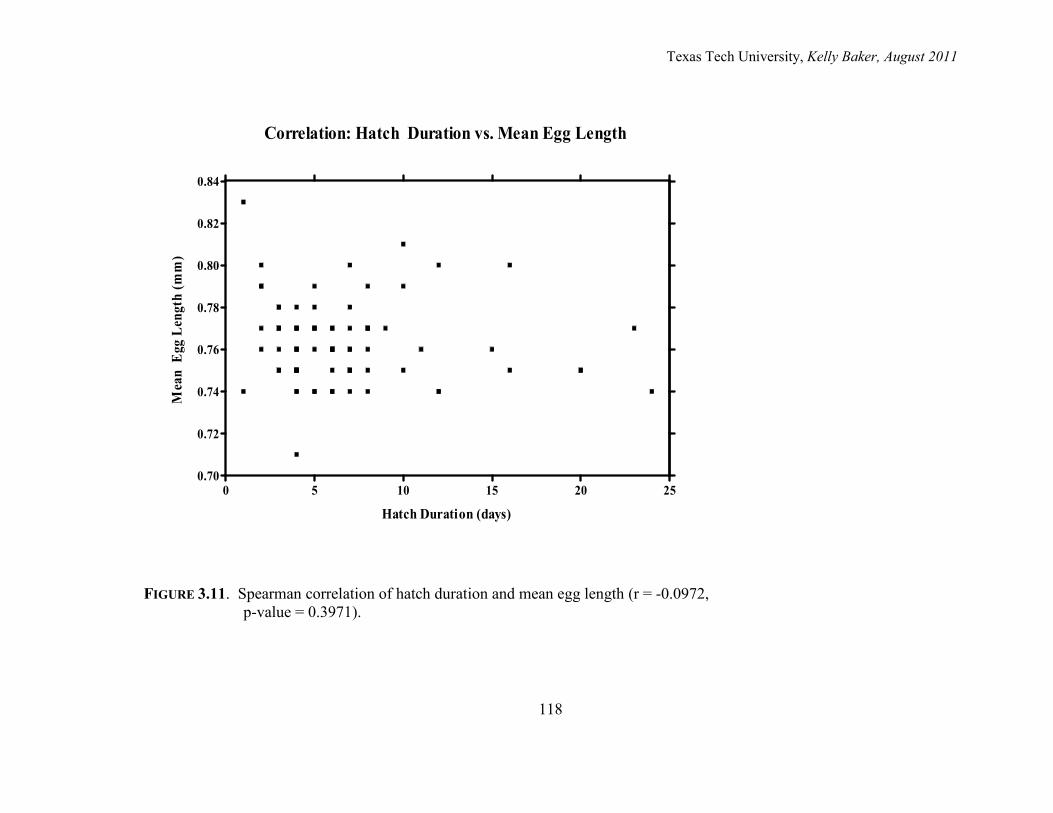
Texas Tech University, Kelly Baker, August 2011
118
Correlation: Hatch Duration vs. Mean Egg Length
0 5 10 15 20 250.70
0.72
0.74
0.76
0.78
0.80
0.82
0.84
Hatch Duration (days)
Mea
n
Eg
g L
eng
th (
mm
)
FIGURE 3.11. Spearman correlation of hatch duration and mean egg length (r = -0.0972,
p-value = 0.3971).

Texas Tech University, Kelly Baker, August 2011
119
Correlation: �umber of Eggs vs. Hatch Success
0 100 200 300 400 500 600 700 800 900 1000 11000.0
0.2
0.4
0.6
0.8
1.0
�umber of Eggs
Ha
tch
S
ucc
ess
(pro
po
rtio
n)
FIGURE 3.12. Pearson correlation of number of eggs and hatch success (r = 0.0551, p-
value = 0.5606).

Texas Tech University, Kelly Baker, August 2011
120
Correlation: Mean Egg Length vs. Hatch Success
0.70 0.72 0.74 0.76 0.78 0.80 0.82 0.840.0
0.2
0.4
0.6
0.8
1.0
Mean Egg Length (mm)
Ha
tch
Su
cces
s (p
orp
ort
ion
)
FIGURE 3.13. Pearson correlation of mean egg length and hatch success (r = 0.2423, p-
value = 0.0337).

Texas Tech University, Kelly Baker, August 2011
121
Correlation: Hatch Duration vs. Hatch Success
0 5 10 15 20 250.0
0.2
0.4
0.6
0.8
1.0
Hatch Duration (days)
Ha
tch
Su
cces
s (p
orp
ort
ion
)
FIGURE 3.14. Pearson correlation of hatch duration and hatch success (r = -0.1858,
p-value = 0.0478).