bakkafjara - sediment transport and morphology - phase …file... · siglingastofnun final report...
TRANSCRIPT

Siglingastofnun Final Report
February 2007
Bakkafjara Sediment Transport and Morphology
Phase 2 Final Report
53551.ibh.jhj.be.02.2007 i DHI Water & Environment
CONTENTS
1 INTRODUCTION ......................................................................................................... 1-1 1.1 Purpose of the Study ................................................................................................... 1-1
2 SELECTION OF MODELLING PERIODS ................................................................... 2-1
3 MODEL INPUT ............................................................................................................ 3-1 3.1 Bathymetry and Harbour Layout.................................................................................. 3-1 3.2 Waves.......................................................................................................................... 3-2 3.2.1 Significant Model Parameters...................................................................................... 3-2 3.2.2 Boundary Conditions ................................................................................................... 3-2 3.2.3 Validation of Wave Predictions .................................................................................... 3-6 3.2.4 Modelling Examples..................................................................................................... 3-6 3.3 Flow ............................................................................................................................. 3-9 3.3.1 Modelling of River Flow ............................................................................................. 3-10 3.3.2 Modelling of Tidal Flow .............................................................................................. 3-12 3.3.3 Modelling Results ...................................................................................................... 3-13 3.4 Sediment Transport ................................................................................................... 3-15 3.4.1 Grain Size and Relative Density ................................................................................ 3-15
4 ANALYSIS OF SEDIMENT TRANSPORT AT OUTER BAR....................................... 4-1 4.1 Period-averaged Sediment Transport Field................................................................. 4-1 4.2 Cross-shore Transport Capacity.................................................................................. 4-2 4.3 Erosion and Deposition Patterns ................................................................................. 4-4 4.4 Sediment Transport Field with Bar Modifications ...................................................... 4-10 4.5 Natural Changes in Bar Depression .......................................................................... 4-15 4.6 Justification of Morphological Model.......................................................................... 4-18
5 WAVES, CURRENTS AND BED LEVELS ALONG NAVIGATION LINE..................... 5-1 5.1 Waves along the Navigation Line and at the Wave Buoy............................................ 5-1 5.2 Currents along the Navigation Line ............................................................................. 5-6 5.3 Waves along the Navigation Line during Selected Storms.......................................... 5-8 5.4 Currents along the Navigation Line during selected Storms...................................... 5-10 5.5 Morphological Changes along Navigation Line ......................................................... 5-12 5.6 Estimated Annual Transports .................................................................................... 5-16
6 COASTAL IMPACT OF BAKKAFJARA PORT FACILITY ........................................... 6-1
7 SEDIMENTATION INSIDE THE HARBOUR ............................................................... 7-1
8 EQULIBRIUM WATER DEPTH IN FRONT OF HARBOUR ENTRANCE.................... 8-1 8.1 Stationary Conditions................................................................................................... 8-1 8.2 Morphological Evolution for Rough South-Westerly Conditions .................................. 8-5 8.3 Morphological Evolution for Rough South-Easterly Conditions ................................... 8-8 8.4 Equilibrium Depth using Capital Dredging at Entrance.............................................. 8-10

53551.ibh.jhj.be.02.2007 ii DHI Water & Environment
8.5 Equilibrium Depth for Different Breakwater Configurations ....................................... 8-13 8.6 Final Comments on the Equilibrium Water Depths.................................................... 8-16
9 SUMMARY .................................................................................................................. 9-1 9.1 Numerical Model.......................................................................................................... 9-1 9.2 Configuration of Harbour ............................................................................................. 9-1 9.3 Sedimentation of Harbour............................................................................................ 9-1 9.4 Outer Bar Morphology ................................................................................................. 9-2
10 REFERENCES .......................................................................................................... 10-1 Appendix A Morphological Changes of February 1989 and November 1985 Appendix B Comparison between Wave Heights along Navigation Line obtained in MIKE
21 SW and Physical Test Model. Appendix C Sea State Information Charts for critical waves Appendix D Sea State Information Charts for 98% waves

53551.ibh.jhj.be.02.2007 1-1 DHI Water & Environment
1 INTRODUCTION
This report presents the Phase 2 modelling investigations and detailed analysis of waves, currents, sediment transport and morphological conditions in the coastal waters located off Bakkafjõru. The study is concerned with the morphological impacts of the planned Bakkafjõru Harbour. The purpose of the harbour is mainly to facilitate the ferry connection to the Vestmannaeyjum. The investigation is conducted using 2D modelling techniques and is a continuation of the work reported in Ref. /1/ - Phase 1 of the present study.
The work reported herein is a full extension of the work reported in the previous Phase 2 progress reports of August and November 2006.
A bird view snapshot of the area of investigation is given in Figure 1.1. The picture shows Bakkafjõru and Vestmannaeyjum (to the right) on the 5th of December 2006.
Figure 1.1 December bird view snapshot of Bakkafjõru coastal region with Markarfljot and Vestman-naeyjum to the right
In the following the English terms for Bakkafjõru and Vestmannaeyjum (i.e. Bakkafjara and Westmann Islands) will be adopted.
1.1 Purpose of the Study
The purpose of the study is to investigate the following morphological aspects:
• Overall stability of the outer bar including the depression in the bar at Bakkafjara and the pit-type (deep trough) morphological feature at Bakkafjara
• Sedimentation rates into the harbour
• Equilibrium depth in front of and in the entrance
These aspects are addressed by the use of coupled numerical 2D models for current, waves and sediment transport. The numerical models are used to simulate the morpho-logical evolution during two (2) characteristic periods.
The surveyed bathymetry of May 2006 is the starting point of all simulations. However, to understand in greater detail the stability of the outer bar, additional morphological

53551.ibh.jhj.be.02.2007 1-2 DHI Water & Environment
simulations are conducted which include the following modifications to the initial bathymetry:
• Placing a pile of sand on the bar in front of the breakwaters • Excavating sand from the bar in front of the breakwaters
• Placing sand in the accumulation zone up-drift of the harbour
To this end the long-term impacts of the harbour on the coastline has been outlined by using a 1D coastline evolution model.
Further, the wave and current conditions along the navigation line have been analysed for critical storms.

53551.ibh.jhj.be.02.2007 2-1 DHI Water & Environment
2 SELECTION OF MODELLING PERIODS
Two distinct periods covering historical storms were modelled to investigate the mor-phological evolution and potential impacts of constructing a harbour at Bakkafjara. Bakkafjara is located on the southern side of Iceland and the number of significant storms are impressive with recorded significant wave heights offshore (63°N, 21°W) reaching nearly 25 m in 1999 (100-year event).
The modelling periods were selected from the analysis of a calculated 27-year time se-ries of waves and longshore transport rates at the site. The time series cover the period 1979-2006 and have a three-hour data-resolution. This history of longshore transport rates was obtained in Ref. /1/ - Phase 1 of the present investigation. The two periods se-lected are:
• November/December 1985 (1/11/85 to 12/12/85) • February 1989 (1/2/89 to 1/3/89) The selected periods cover approximately 70 days in total.
The selected periods include 3 major storms i.e. storms that are placed in the Top-20 of the most important storms in terms of wave exposure (see Table 1 of Ref. /1/). The pe-riods include two storms in November 1985 where waves exceed 8 m for approximately 66 hours in the offshore region. During one of the storms the mean wave direction was south-easterly. The 1989 February storm had 30 hours of waves above 8 m and the mean wave direction was here south-westerly. The selected periods thus include both severe south-easterly and south-westerly storms.
The wave roses for the offshore waves (63°N 21°W) are presented in Figure 2.1.
Figure 2.1 Offshore wave conditions for November 1985 (left) and February 1989 (right)
53551.ibh.jhj.be.02.2007 2-2 DHI Water & Environment
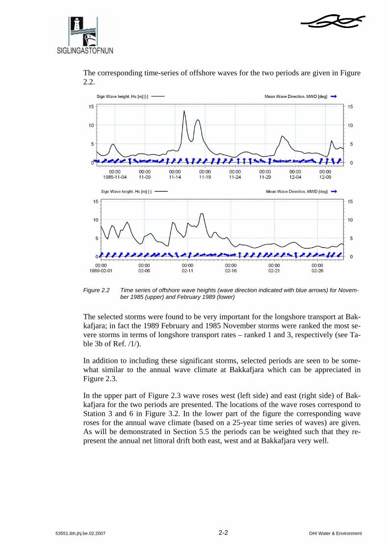
The corresponding time-series of offshore waves for the two periods are given in Figure 2.2.
Figure 2.2 Time series of offshore wave heights (wave direction indicated with blue arrows) for Novem-ber 1985 (upper) and February 1989 (lower)
The selected storms were found to be very important for the longshore transport at Bak-kafjara; in fact the 1989 February and 1985 November storms were ranked the most se-vere storms in terms of longshore transport rates – ranked 1 and 3, respectively (see Ta-ble 3b of Ref. /1/).
In addition to including these significant storms, selected periods are seen to be some-what similar to the annual wave climate at Bakkafjara which can be appreciated in Figure 2.3.
In the upper part of Figure 2.3 wave roses west (left side) and east (right side) of Bak-kafjara for the two periods are presented. The locations of the wave roses correspond to Station 3 and 6 in Figure 3.2. In the lower part of the figure the corresponding wave roses for the annual wave climate (based on a 25-year time series of waves) are given. As will be demonstrated in Section 5.5 the periods can be weighted such that they re-present the annual net littoral drift both east, west and at Bakkafjara very well.

53551.ibh.jhj.be.02.2007 2-3 DHI Water & Environment
Figure 2.3 Upper: wave climate west and east of Bakkafjara for the modelled periods. Lower: annual wave climate west and east of Bakkafjara (based on 25 years of waves). Locations west and east of Bakkafjara correspond to Station 3 and 6 in Figure 3.2.

53551.ibh.jhj.be.02.2007 3-1 DHI Water & Environment
3 MODEL INPUT
The modelling of waves, flow, sediment transport and morphological evolution is done using the coupled MIKE 21 FM model. The model calculates waves (MIKE 21 SW), flow (MIKE 21 HD), sediment transport and morphological evolution (MIKE 21 ST) on an unstructured mesh and in a sequential and fully integrated manner.
3.1 Bathymetry and Harbour Layout
In Figure 3.1 the unstructured mesh and the model bathymetry with the proposed Bak-kafjara Harbour breakwaters are presented. The model bathymetry is derived from water depths obtained during the bathymetrical survey of May 2006.
The wave, flow and sediment transport description is refined towards the area of inter-est. In the vicinity of the harbour the resolution of the bathymetry is increased to ≅ 50 m2 (the high resolution area includes part of the trough and bar). The relatively large model area (covers 14 km in the alongshore direction) is crucial for describing the alongshore variation in wave height which the Westmann Islands are responsible for.
The variation in wave height along the coastline is important for generating the so-called rip-current at Bakkafjara correctly. A detailed explanation of the rip current and its impact on the morphology will be given later.
Figure 3.1 Model bathymetry (local model) based on the survey of May 2006
The harbour or ferry port is implemented as streamlined breakwaters with the entrance facing the sea. The width of the entrance (from the foot of the breakwater to the foot of the breakwater) is 100 m and the entrance is located at a (undisturbed) water depth of 8.0 m. Recent refined assessments of the channel width suggest that an entrance width

53551.ibh.jhj.be.02.2007 3-2 DHI Water & Environment
of approximately 86 m is sufficient. In the present model set-up the width of the en-trance has an impact on the harbour sedimentation only. The impact of different en-trance widths will be addressed separately in Section 7 dealing with sedimentation of the harbour.
In Section 8 an investigation of the equilibrium depth in the entrance area is presented. Water depths here are determined by various factors including the configuration of the harbour and in particular the outer part of the breakwaters. The optimal configuration of the outer part of the breakwaters has been investigated and it turns out that the outer part of the western and eastern breakwater should be aligned such that the angle between them is approximately 65°.
3.2 Waves
A fully spectral wave model, MIKE 21 SW, has been used to simulate the propagation of waves. The model includes all relevant wave phenomena such as shoaling, breaking, refraction, and local wind generation.
3.2.1 Significant Model Parameters The model uses the wave breaking method of Ruessink, Ref /4/, which is an elaboration of the model by Battjes and Janssen. Applied wave-breaking parameters in the model of Ruessink are: γ2=0.6 and α=0.55. The model parameters are determined after calibration against field measurements as well as physical model test including detailed surf zone information.
The waves are calculated on the flexible computational mesh shown in Figure 3.1. The model calculates the distribution of wave height, wave periods, wave direction and spreading of waves and calculates radiation stresses which drive the longshore current.
3.2.2 Boundary Conditions The transformation of waves from the offshore location (63°N, 21°W) to the boundary of the local model (see Figure 3.1) is done by running the regional wave model de-scribed in Ref. /1/ and extracting wave parameters at several positions along a line cor-responding to the boundary of the local model. The wave parameters vary significantly along the boundary of the local model area due to shadow effects of Westmann Islands. Wave conditions at 6 locations along the line corresponding to the boundary of the local model are extracted - see Figure 3.2 where wave conditions at locations 3 to 8 are used as boundary conditions in the local model.

53551.ibh.jhj.be.02.2007 3-3 DHI Water & Environment
Figure 3.2 Extraction points for near-shore wave time series
In Figure 3.3 and Figure 3.4 wave roses at positions 2, 3, 4, 5, 6 and 7 (see Figure 3.2) are given for the modelling periods.

53551.ibh.jhj.be.02.2007 3-4 DHI Water & Environment
Figure 3.3 Wave roses for November 1985 along the boundary of the local model. Upper wave roses: position 2 and 3.Wave roses in middle: position 4 and 5. Lower wave roses: position 6 and 7. Positions are shown in Figure 3.2

53551.ibh.jhj.be.02.2007 3-5 DHI Water & Environment
Figure 3.4 Wave roses for February 1989 along the boundary of the local model. Upper wave roses: position 2 and 3.Wave roses in middle: position 4 and 5. Lower wave roses: position 6 and 7. Positions are shown in Figure 3.2

53551.ibh.jhj.be.02.2007 3-6 DHI Water & Environment
3.2.3 Validation of Wave Predictions The combined regional wave transformation model and local wave model are validated against measured waves from the Bakkafjara wave buoy. The Bakkafjara wave buoy was deployed 18 November 2003 and has measured wave heights and wave periods continuously ever since. The wave buoy is located on approximately 28 m water west of the proposed Bakkafjara Harbour (see Figure 5.1). The selected validation period is March 2004. During March 2004 the wave heights were among the largest recorded.
In Figure 3.5 the comparison between modelled and measured wave heights at Bak-kafjara wave buoy is presented. It can be seen that the considerable wave height reduc-tion taking place from offshore (south of Westmann Islands) to the location of the wave buoy is captured correctly by the model and, more essentially, all important spikes and lows found in the measured waves are well captured by the model.
Figure 3.5 Comparison between modelled (red dots) and measured (blue line) wave heights at Bak-kafjara wave buoy, March 2004. The offshore wave heights are shown for comparison (black dots)
When rotating the wave directions applied on the boundary of the local wave model (wave directions along the boundary of the local model are shifted clockwise or anti-clockwise) the wave model gives wave heights at the buoy that do not compare as well as that presented in Figure 3.5, suggesting that the applied wave directions must be close to measured wave directions. Although wave directions are not measured at this location it can be argued that measured wave directions are not required as part of the present model validation given the fine comparison presented in Figure 3.5.
3.2.4 Modelling Examples The effect on the distribution of wave heights (significant) of Westmann Islands (Vest-mannaeyjum) is pronounced for south-westerly waves. An example of the pronounced sheltering effect of the Westmann Islands is given in Figure 3.6. In Figure 3.7 the shel-tering effect for waves from south and south-east is given as well.

53551.ibh.jhj.be.02.2007 3-7 DHI Water & Environment
Figure 3.6 Upper: wave field in regional wave model with waves from south-west. Notice the extensive sheltering provided by the Westmann Islands. Lower: bird-view of Westmann Islands

53551.ibh.jhj.be.02.2007 3-8 DHI Water & Environment
Figure 3.7 Upper: wave field in regional wave model with waves from south. Lower: wave field in re-gional wave model with waves from south-east
In Figure 3.8 snapshots of the wave transformation in the local model for cases where waves approach from south-west (upper) and south-east (lower) are presented. Colours give the significant wave height whereas vectors show the mean wave direction (length of vector is proportional to wave height).

53551.ibh.jhj.be.02.2007 3-9 DHI Water & Environment
Figure 3.8 Snapshots of wave fields (significant wave heights) during the February 1989 storm. Upper: waves from south-west. Lower: waves from south-east
3.3 Flow
The MIKE 21 HD has been used to calculate the flow. MIKE 21 HD is a general nu-merical modelling system for simulating water levels and velocities in estuaries, bays and coastal areas. It simulates unsteady flows using depth integrated formulation (2D flow equations).
The MIKE 21 HD includes formulations for the effects of:
• Convective and cross momentum • Bottom shear stress • Wind shear stress at the surface • Wave driven currents through the radiation stresses (obtained every time step
from MIKE 21 SW) • Coriolis forces • Momentum dispersion (through e.g. the Smagorinsky formulation)

53551.ibh.jhj.be.02.2007 3-10 DHI Water & Environment
• Sources and sinks (mass and momentum) • Flooding and drying The solution is obtained with the finite volume approach on the triangular mesh pre-sented in Figure 3.1.
3.3.1 Modelling of River Flow The discharge from the river Markarfljot located approximately 2.5 km east of Bak-kafjara is included in the hydrodynamical set-up. The river carries a significant amount of sediment which is sourced into the coastal zone during periods of heavy run-off and thus plays an important role in determining the morphological development. Markarfljot is very dynamic. Historic observations show that the location of the river mouth is shift-ing continuously. A bird view of the Markarfljot river outlet and the lower part of its river plain is shown in the upper part of Figure 3.9. The pronounced meandering and braiding of the river is a clear indication of the dynamic nature of Markarfljot river. In the lower part of Figure 3.9 the Markarfljot is viewed from the coastal plain itself and up river. Several active water falls (providing the river with water) are seen along the adjacent cliff (east of the river).
Figure 3.9 Markarfljot 5th December 2006. Note scattered water falls along the cliff in the picture below
The annual discharge at the river mouth from 1961 to 2001 has been calculated and evaluated in Ref. /3/. The average discharge was found to be 96 m3/s but with signifi-cant seasonal variations. The peak discharge during the large flood of January 11th, 2002 was estimated to 1500 m3/s.
The discharge during simulated periods is presented in Figure 3.10 and Figure 3.11 (from Ref. /3/).

53551.ibh.jhj.be.02.2007 3-11 DHI Water & Environment
The amount of sand sourced to the coastal zone from Markarfljot river has a significant impact on the coastal sediment budget. The influence on the coastal morphology can be seen from the morphological calculation presented in Section 4. The amount of sedi-ment carried by the river is calculated by MIKE 21. The sediment carried into the coastal zone during the two simulated periods is shown in Figure 3.10 and Figure 3.11. The accumulated sediment load is shown as well. It can be seen that nearly 20,000 m3 sand was discharged from the river during November/December 1985. During February 1989 approximately 10,000m3 sand was discharged.
Figure 3.10 River discharge and sediment load during November 1985. Upper: river mouth discharge (Markarfljot) – From Ref. /3/. Lower: sediment load and accumulated sediment load

53551.ibh.jhj.be.02.2007 3-12 DHI Water & Environment
Figure 3.11 River discharge and sediment load during November 1989. Upper: river mouth discharge (Markarfljot) – From Ref. /3/. Lower: sediment load and accumulated sediment load.
The calculated sediment load depends among other things on the river discharge, the grain size and the profile of the river cross-section. Both grain sizes and river discharges are well-documented. The profile of the river cross-section (i.e. the depth) is, however, unknown. During the 70 days of simulation the discharge of sand from the river was 30,000 m3. The annual discharge of sand based on the simulated periods is therefore es-timated to be 150,000 m3 which is close to the well-known value of 100,000 m3 (see Ref. /1/). The profile used in the model bathymetry is thus considered to be suitable.
3.3.2 Modelling of Tidal Flow Forecasted tidal elevations and velocities from March 2004 were made available at 8 positions just off Bakkafjara. The forecasted tidal elevation and velocity are extracted from a tidal model which is run on an operational basis at the Icelandic Maritime Ad-ministration to predict sea level and tidal currents in Icelandic coastal waters using a weather forecast from the European Centre for Medium Range Weather Forecasts. The model is refereed to as the IMA model. The flow model, MIKE 21 HD, was calibrated to reproduce current speeds and surface elevations from IMA’s model.
In Figure 3.12 surface elevations and current speeds at a water depth of 10 m from MIKE 21 and from IMA’s model are compared for a full spring-neap period, March 2004. Very good comparisons for the surface elevations are seen.

53551.ibh.jhj.be.02.2007 3-13 DHI Water & Environment
Figure 3.12 MIKE 21 model results (black line) and forecasted results from the Icelandic Maritime Ad-ministration (blue dots) surface elevation [m] (upper) and current speed [m/s] (lower) at wa-ter depth 10 m. Period: March 2004
3.3.3 Modelling Results In Figure 3.13 snapshots of the current fields (dominating currents are driven by radia-tion stresses) for cases where waves approach from south (upper) and south-west (lower) in the area near Bakkafjara are presented. The colours indicate the speed of the depth-averaged velocity whereas the vectors show the direction of the current (length of vector is proportional to the speed).
The snapshot situation with waves from south gives strong currents that are directed away from Bakkafjara and currents are strongest on the open coast west of Bakkafjara. The change in current direction is due to the distinctive change in coastline orientation at Bakkafjara.
The snapshot in the lower part of the figure demonstrates the shadow effect of West-mann Islands on the longshore current. The current attenuates along the bar and is weak east of Bakkafjara.

53551.ibh.jhj.be.02.2007 3-14 DHI Water & Environment
Figure 3.13 Bathymetry (May 2006) and snapshots of typical current fields

53551.ibh.jhj.be.02.2007 3-15 DHI Water & Environment
3.4 Sediment Transport
The wave/current induced sediment transport and the associated morphological evolu-tion in the study area were obtained by DHI´s MIKE 21 ST. The transport rates and the morphological evolution are calculated on the flexible mesh presented in Figure 3.1.
The sediment transport is calculated every time step using the information from MIKE 21 SW (wave height, periods, directions, spreading) and MIKE 21 HD (currents, water levels).
The model requires information on mean grain size, the standard deviation and relative density of the sand. The sand at Bakkafjara is known to have a high density which is typical for basalt sand – see Figure 3.14.
Figure 3.14 Example of the dark basalt sand which is characteristic at Bakkafjara
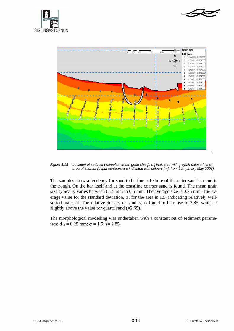
3.4.1 Grain Size and Relative Density An extensive number of sediment samples were collected in the vicinity of the proposed harbour along lines perpendicular to the coastline. The positions of the samples are shown on top of the bathymetry. Figure 3.15 also displays the measured mean grain size (the mean grain size is indicated in a palette of light to dark gray).
53551.ibh.jhj.be.02.2007 3-16 DHI Water & Environment
¨
Figure 3.15 Location of sediment samples. Mean grain size [mm] indicated with greyish palette in the area of interest (depth contours are indicated with colours [m], from bathymetry May 2006)
The samples show a tendency for sand to be finer offshore of the outer sand bar and in the trough. On the bar itself and at the coastline coarser sand is found. The mean grain size typically varies between 0.15 mm to 0.5 mm. The average size is 0.25 mm. The av-erage value for the standard deviation, σ, for the area is 1.5, indicating relatively well-sorted material. The relative density of sand, s, is found to be close to 2.85, which is slightly above the value for quartz sand (=2.65).
The morphological modelling was undertaken with a constant set of sediment parame-ters: d50 = 0.25 mm; σ = 1.5; s= 2.85.

53551.ibh.jhj.be.02.2007 4-1 DHI Water & Environment
4 ANALYSIS OF SEDIMENT TRANSPORT AT OUTER BAR
In the following the sediment transport field and the morphological evolution during the selected periods are presented. The following items are covered:
• Period-average transport fields for the selected periods
• Role of cross-shore transport during the selected periods
• Morphological evolution (erosion/deposition patterns) with focus on the navigation line and the bar depression
The main focus of this section is devoted to the understanding of the dynamics of the outer bar. It is well-known that the water depth along the outer bar changes with a maximum in water depth at a location near Bakkafjara. This depression in the outer bar is a persistent feature and confirmed by historical records as well as more detailed sur-veys conducted during the past 6 years. Recent surveys show, however, that the scale size of the depression in the outer bar changes. During the past 6 years the water depth over the depression has changed considerably. The explanation for these changes and the morphological behaviour in general will be investigated using a combination of the modelling results and the comprehensive measurements available at this site.
4.1 Period-averaged Sediment Transport Field
In Figure 4.1 and Figure 4.2 the period-averaged sediment transport fields for the No-vember 1985 and February 1989 storm are depicted.
Both periods include waves from south-westerly and south-easterly directions; however, the main storm in November 1985 is south-easterly dominated. The overall trend in the November 1985 sediment transport field is that sediment is seen to be transported to the west, west of Bakkafjara and to the east, east of Bakkafjara. The important aspect of this is that the point of inflexion (divergence in sediment transport) is located over the bar depression which is found just east of the proposed ferry port. Thus, during this period, or more generally, periods of south-easterly storms, the depression in the bar is main-tained.
The overall trend in the February 1989 sediment transport field is that sediment is seen to be transported to the east. Sediment is thus transported by the longshore current on the outer bar to the bar depression. Normally, this would entail a deterioration of the bar depression, however, looking more closely at the transport field it is realised that a small offshore deflection in the transport direction is induced. The physical explanation of the deflection is discussed in more detail later; however, the impact of such deflec-tion in the transport direction is that the bar-depression is preserved.
Thus, simulation of the two periods clearly reveal mechanisms that maintain the bar de-pression.

53551.ibh.jhj.be.02.2007 4-2 DHI Water & Environment
Figure 4.1 Period-averaged transport field for November 1985 storm
Figure 4.2 Period-averaged transport field for February 1989 storm
4.2 Cross-shore Transport Capacity
The sediment transport results presented above were obtained with a sediment transport description which is based on depth integrated flow patterns such that the direction of the sediment transport was assumed to be in the direction of the depth-averaged flow. In this section sediment transport associated with complex 3D flow patterns are evaluated over a fixed bed. This is done as 3D flows in the surf zone mobilise cross-shore trans-ports, examples of mechanisms that induce such transport are:
• Streaming in the wave boundary layer and wave drift • Undertow • Net bed shear stress from asymmetrical waves

53551.ibh.jhj.be.02.2007 4-3 DHI Water & Environment
• Wave-current motion (produce net cross-shore transports due to wave-current non-linearity)
• Helical motion from centrifugal forces
Although transport rates induced by these mechanisms are small compared to the along-shore transport rates they govern the shape of the cross-shore profile and thus the cross-shore motion of the bar. These mechanisms must be accurately balanced in the model to avoid biased cross-shore transports and a degeneration of the coastal profile. In the pre-sent case the cross-shore motion of the bar is not of paramount significance as bathy-metrical surveys indicate that the distance from the bar to the coastline is fairly constant. Omitting the mechanisms in the sediment transport description attached to the morpho-logical model is thus justified.
In the following, sediment transports generated by 3D flow mechanisms are evaluated. Figure 4.3 presents the sediment transport component normal to the depth-averaged flow. The sediment transports normal to the depth-averaged flow is associated with the 3D mechanisms mentioned above. The sediment transport shown in Figure 4.3 is the pe-riod-averaged sediment transport (averaged over the modelling period i.e. February 1989). The period-averaged transport field presented in Figure 4.3 is thus in addition to that shown in Figure 4.2 which is the transport in the direction of the depth-averaged flow.
It is seen that 3D mechanisms induce a transport normal to the flow direction which on the bar is onshore directed. Off the crest of the bar and close to the coastline where waves are breaking the transport normal to the flow direction is offshore directed (due to undertow). Behind the bar in the trough the transport turns onshore again. The pe-riod-averaged cross-shore transport pattern will tend to widen the outer bar of May 2006.
The period-averaged cross-shore transport along the bar is seen to reduce towards the depression. This is due to the smaller wave action in the sheltered zone. On the east side of the depression the period-averaged cross-shore transport is even seen to be onshore directed.
Close to the depression in the bar the offshore directed transport is larger than elsewhere on the bar whereas the bar east of the depression has an onshore directed transport.
The net 3D transports are, however, small (in the order of 5 m3/m/year) and are not likely to be responsible for the shaping of the bar depression.

53551.ibh.jhj.be.02.2007 4-4 DHI Water & Environment
Figure 4.3 Period-averaged transport field associated with 3D flow mechanisms (transports normal to the depth-averaged flow). Period: February 1989 storm
4.3 Erosion and Deposition Patterns
In Figure 4.4 and Figure 4.5 the modelled erosion/deposition pattern (based on depth in-tegrated flow) for the two periods is presented. The erosion/deposition maps are also given in higher resolution in Appendix A. Isolines in Figure 4.4 and Figure 4.5 and Ap-pendix A are taken from the initial bathymetry whereas the colours are bathymetries at the end of the modelling periods. By comparing the isolines with the colours the mor-phological evolution can be identified.
The following important morphological activity has taken place during November 1985:
• Accretion of sediment near the river outlet (between 0 m and -2 m)
• Deposition of sediment near the breakwaters (between 0 m and -6 m) especially on the east side. The coastline has advanced approximately 60 m on the east side
• No significant changes in the deep trough located between the harbour mouth and the bar are seen
• Changes at water depths up to 14 m, i.e. along the outer side of the bar
• Only small changes in navigation depth in the mouth of the breakwaters (see also Figure 5.13)
53551.ibh.jhj.be.02.2007 4-5 DHI Water & Environment
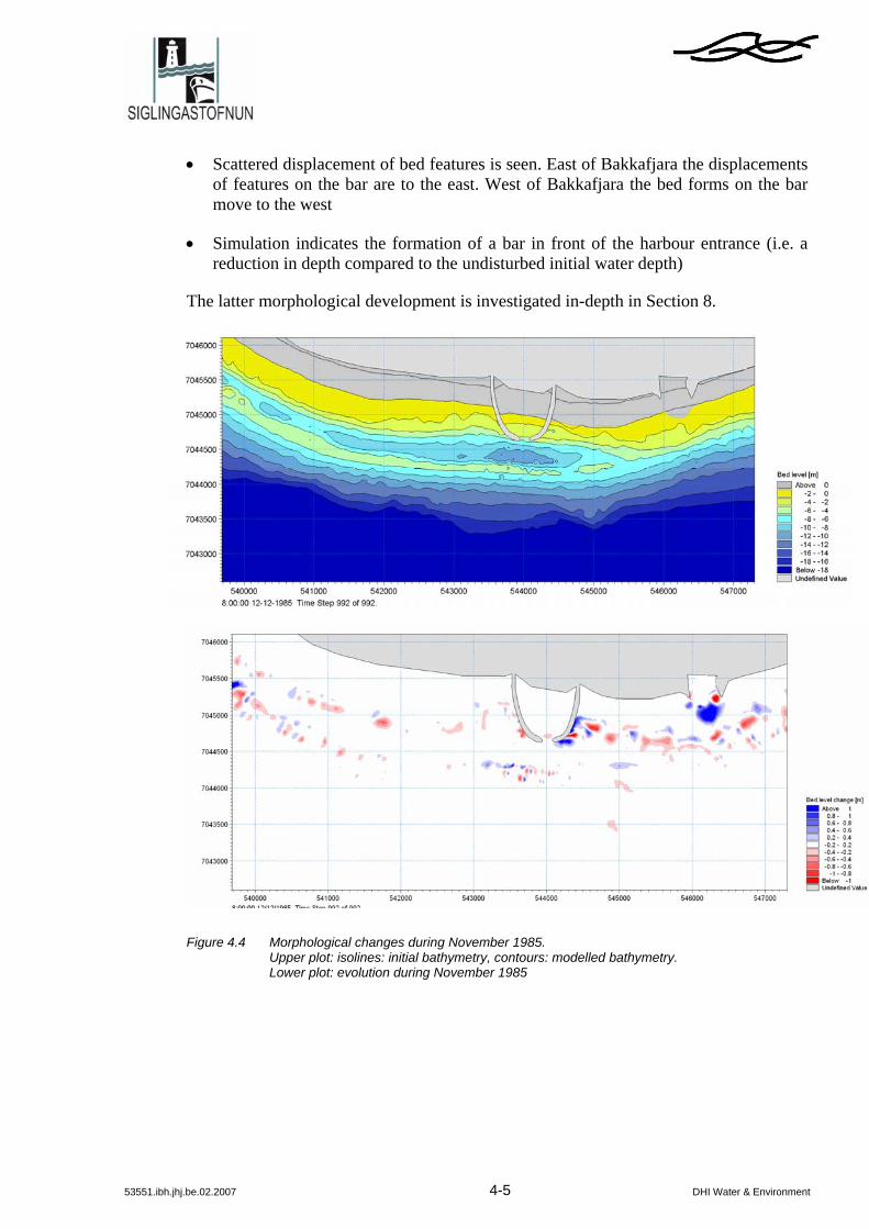
• Scattered displacement of bed features is seen. East of Bakkafjara the displacements of features on the bar are to the east. West of Bakkafjara the bed forms on the bar move to the west
• Simulation indicates the formation of a bar in front of the harbour entrance (i.e. a reduction in depth compared to the undisturbed initial water depth)
The latter morphological development is investigated in-depth in Section 8.
Figure 4.4 Morphological changes during November 1985. Upper plot: isolines: initial bathymetry, contours: modelled bathymetry. Lower plot: evolution during November 1985

53551.ibh.jhj.be.02.2007 4-6 DHI Water & Environment
The following important morphological activity has taken place during February 1989:
• Accretion of sediment near the river outlet (between 0 m and -2 m) with a clear dis-placement of the sand towards east
• Deposition of sediment near the breakwaters (between 0 m and -6 m). The coastline has advanced approximately 50 m and 35 m on the east and west side of the break-water, respectively
• Small changes in the deep trough located between the harbour mouth and the bar are seen
• Deposition on the bar to the west of the harbour
• General erosion to the east of the harbour out to the -6 m contour
• Tendency for lowering of the bar in front of the breakwaters
• Very small changes in the navigation depth in the mouth of the breakwaters (see also Figure 5.13).
• Simulation indicates the formation of a bar in front of the harbour entrance (i.e. a reduction in depth compared to the undisturbed depth)
The latter morphological development will be investigated in even more detail in Section 8.

53551.ibh.jhj.be.02.2007 4-7 DHI Water & Environment
Figure 4.5 Morphological changes during February 1989 Upper plot: isolines: initial bathymetry, contours: modelled bathymetry. Lower plot: evolution during February 1989
The tendency of the outer bar to break up while being eastwardly displaced under condi-tions with eastward transport is worth noting. These changes in the morphological pat-tern are due to the seaward deflection in the transport briefly mentioned in the previous section. The deflection of sediment on the outer bar is caused by a cross-shore transport mechanism; a mechanism which is pronounced at the location of the bar depression (i.e. at Bakkafjara). In Section 4.2 period-averaged transports perpendicular to the depth-averaged flow originating from 3D flow phenomena are presented; however, these do not show particularly pronounced cross-shore transports at the bar depression. In Figure 4.6 instantaneous sediment transport patterns are shown for conditions with strong east-ward transport. The figure shows that while sediment is moving parallel with the bed contours both east and west of Bakkafjara, a considerable deflection of the transport (compared to the contours of the bar) at Bakkafjara is seen. The deflection of sediment can be caused by several mechanisms; however, most likely is the formation of a rip-type current. Such current is likely to form at the site. Rip currents are generated due to alongshore variations in the set-up (from wave breaking). On an open coastline rips are

53551.ibh.jhj.be.02.2007 4-8 DHI Water & Environment
normally caused by variations in the height of the bar and are very mobile. In the pre-sent case the mechanism can be caused by the variation in the wave height. A variation in the wave height is seen due to the shadow effect of Westmann Islands. Behind the Westmann Islands waves are smaller and consequently the set-up here is reduced. This gives an alongshore gradient in the surface elevation driving a current. This current is in addition to the longshore current. The current turns seaward at the point of the smallest set-up. The location of the smallest set-up varies with the direction of the wave such that the location where sediment is being pushed seaward by the rip changes.
Figure 4.6 Instantaneous transport profiles along the Bakkafjara coastline (storm, February 1989)
The magnitude of the rip current is controlled by the gradient in the surface elevation. In Figure 4.7 the surface elevation for conditions with waves from south-west and south is depicted. The figure clearly shows the variation in water level along the coastline with south-westerly waves changing from 1.4 m at approximately 4 km west of Bakkafjara to around 1.15 m in the sheltered area near Bakkafjara. The difference in surface elevation is approximately 25 cm which is of a magnitude fully capable of driving a relatively strong current. For the southerly waves the gradient increases even further with a change in surface elevation 30 cm over 800 m.

53551.ibh.jhj.be.02.2007 4-9 DHI Water & Environment
Figure 4.7 Surface elevation under south-western (upper) and southern (lower) storm conditions. Col-ours: surface elevation. Isolines: bathymetry
The rip-current will maintain a depression in the outer bar; however, the dimensions of the depression are a function of the wave height and wave direction. The dimensions are determined by the continuous “battle” between the scouring effect of the rip current and the infill of sediment transported by the longshore current along the outer bar on the up-drift side and erosion on the down-drift side. The longshore current is strongest when the wave angle is 45 degrees to the coastline and weakest when waves attack perpen-dicularly, thus dominant rip scouring may be expected when the waves approach from south-south-west.
The mechanism is not limited to south-westerly wave conditions. It can be initiated dur-ing southerly storms as well – see Figure 4.7.
An alternative morphodynamical simulation of the 1985 period is made with a speed-up factor on the morphological development of 25 (this means that the morphology at the

53551.ibh.jhj.be.02.2007 4-10 DHI Water & Environment
end of the period would correspond to that of 25 of the same periods). The result is shown in Figure 4.8. The accelerated simulation shows the formation of a rip-channel – see the marking in Figure 4.8. The scoured rip channel is similar to that seen in the Oc-tober 2002 bathymetry – see Figure 4.8.
Figure 4.8 Bathymetry after 25 periods corresponding to that of the 1985 period (upper). Note the scoured rip channel inside circle. Such rip channel can be seen in the surveyed October 2002 bathymetry (below) as well
4.4 Sediment Transport Field with Bar Modifications
To further understand the morphological features and governing processes at Bakkafjara the bathymetry is modified considerably. Once exposing the modified bathymetry to the forcing of the selected periods the bathymetry will return to its original shape, however, the mechanisms responsible for the reshaping are important.
The morphological development of the bar in the cases where
• a pile of sand is placed on the bar and in front of the breakwaters, • sand has been excavated from the bar in front of the breakwaters

53551.ibh.jhj.be.02.2007 4-11 DHI Water & Environment
is investigated with the morphological model for February 1989. The modifications of the outer bar are made in the vicinity of the navigation line and such that the water depth over the bar is reduced to 2 m over approximately 300 m in the alongshore direc-tion in the first mentioned case. The water depth over the bar in the case where the bar has been excavated is increased to 7 m over a distance of 150 m. In Figure 4.9 the model bathymetry with the described modifications in the morphology are shown. In Figure 4.10 the period-averaged sediment transport over the 1989 storm is presented for the morphological alterations described above.
Figure 4.9 Model bathymetry for morphology with deposition on bar (left) and excavation of bar (right)
Sediment transport fields for February 1989 are shown in Figure 4.10 and Figure 4.11. In the upper part of Figure 4.10 the period-averaged transport for the case where the depth is reduced is shown and in the lower part a snap-shot of the transport field is shown. In the upper part of Figure 4.11 the period-averaged transport for the case where sand has been excavated is shown and in the lower part a snap-shot of the transport field is shown. The snap-shots are presented to illustrate the transport processes along the outer bar. During periods of moderate longshore transports the processes are easily identified.
The period-averaged transport for February 1989 is seen to be affected significantly by the crest elevation of the bar near the navigation line. In the case of low-water-depths-over-bar the morphology is very active. The combined effort of flow and waves causes the pile of sand to erode. The eroded sand is seen to be transported landward. The rea-son for the landward transport is due to the flow induced by the more intense wave breaking over the elevated part of the bar.

53551.ibh.jhj.be.02.2007 4-12 DHI Water & Environment
Figure 4.10 Upper: period-averaged transport field (scaling on vectors as in Figure 4.2) for morphology with bar deposition. Lower: snap-shot of transport field
In the case where the bar is excavated the bar morphology is less active compared to the situation where sand has been deposited. However, the level of the excavation is seen to be maintained with a slight tendency for further deepening. Sand is seen to be trans-ported seaward. The reason for the seaward transport is due to the rip current induced by the less intense wave breaking over the lower part of the bar.

53551.ibh.jhj.be.02.2007 4-13 DHI Water & Environment
Figure 4.11 Upper: period-averaged transport field (scaling on vectors as in Figure 4.2) for morphology with bar deposition. Lower: snap-shot of transport field
The morphological changes for the two cases are presented in Figure 4.12. The water depth along the original bar is nearly re-established (during one month) at approxi-mately 5 m. Eroded sand has not been supplied to the bar east of the pile. The pile has simply moved landward reducing the volume of the deep pit-type trough located in front of the harbour entrance.
In the case of the excavated bar it is seen that the excavation is displaced in the eastward direction by approximately 70 m (the 6 m contour line). The water depth in the central part of the excavation is increased by 10-20 cm over the period. This case shows exactly the two mechanisms at play. The resulting level of the bar is a continuous battle be-tween the rip current induced erosion and the deposition of sand caused by the long-shore current. The present storm is seen to displace the depression eastward and al-though the water depth over the depression is increased the depth at the navigation line is decreased.

53551.ibh.jhj.be.02.2007 4-14 DHI Water & Environment
Figure 4.12 Morphological changes during February 1989 with isolines showing initial bathymetry and contours showing modelled bathymetry.
Upper plot: deposition on bar Lower plot: excavation of bar
The simulations with the modified bathymetries clearly demonstrate that the cross-shore transport related to depth integrated currents over the outer bar at Bakkafjara is respon-sible for the existence of the depression. In the case of sand being piled up on the outer bar the shoreward transport mechanism is seen to be very dominating. The pile is eroded and the material is disposed behind the bar. In the case of excavating part of the outer bar the bar is more stable implying that the excavated area with water depth of 7m is closer to being in equilibrium with the forcing conditions of the selected period.
This investigation shows that the depression in the outer bar is a persisting feature in the morphology and that the reason for the depression is the transport induced by along-shore variation in the wave set-up.

53551.ibh.jhj.be.02.2007 4-15 DHI Water & Environment
4.5 Natural Changes in Bar Depression
In above sections the relationship between the sheltering effect of the Westmann Islands (inducing a rip current) and the presence of a depression in the outer bar at Bakkafjara has been made evident through numerical modelling. In this section the historical data is revisited and the rip-current hypothesis is tested.
In Figure 4.13 a time-series showing annually averaged wave energy and wave direc-tions for the period 1958 to 2006 at the offshore location (63°N, 21°W) is plotted. In Figure 4.14 the wave height averaged over 4 and 8 years is presented. From these plots the following observations can be made:
• The annually averaged wave energy (green line) is seen to vary with a factor of up to 3 from one year to the next
• The average offshore wave direction (red line) has since 2002 been south-westerly and the average level of wave energy has been around the mean value for the period
• The running average indicates return periods in the order of 8-10 years
Figure 4.13 Time series of annually averaged wave energy (green) and wave directions (red and black) at an offshore location (63°N, 21°W). Water depth over the bar depression is shown in blue

53551.ibh.jhj.be.02.2007 4-16 DHI Water & Environment
Figure 4.14 Time series of (running) averaged wave energy (green) and wave directions (red and black) at an offshore location (63°N, 21°W). The averaging is performed over: Top: 4 years. Bot-tom: 8 years
To supplement the time-averaged wave-energy and wave directions presented above, the minimum water depth over the outer bar (at the position of the navigation line) is given in Figure 4.15. These depths are based on the bathymetrical surveys conducted annually since 2002. The water depth over the outer bar at the navigation line deterio-rated in the period from 2002 to 2006. The most recent bathymetric survey from Janu-ary 2007 shows a clear increase in the minimum water depth, however.
Figure 4.15 Water depth at the outer bar at the position of the navigation line

53551.ibh.jhj.be.02.2007 4-17 DHI Water & Environment
A variation in water depths of approximately 2 m over the past 5 years is not surprising considering the large variability in the offshore wave direction and wave energy. Shal-low water depths (over the outer bar depression) were seen in the May 2006 bathymetry whereas large water depth was seen in the October 2002 bathymetry.
If the October 2002 bar morphology (where the outer bar water depths were the largest surveyed so far) is studied closely (see Figure 4.8) a very distinct difference compared to latter bathymetries can be recognized namely that the eastern side of the deep trough is seen to scour the outer bar. In later surveys the trough is seen to be located behind the outer bar. The question is what makes the October 2002 bathymetry different? If the wave and sediment transport climate a few months prior to the 2002 survey is studied the following interesting conditions can be identified:
• Two (2) very significant storms were observed west of Bakkafjara. Both these storms were among the 6 most severe storms in terms of wave exposure (in the pe-riod from 1979 to 2004). This is documented in Table 2a, Ref. /1/
• These storms did not give rise to longshore transport rates that match the severity in terms of wave exposure. In fact both storms did not produce longshore transport rates in the Top 20 – see Table 2b, Ref. /1/
• These storms did not produce significant wave exposure or longshore transport rates at Bakkafjara – see Table 3a and 3b, Ref. /1/
Storms that have the combination of great wave exposure west of Bakkafjara, small wave exposure at Bakkafjara and relatively low rates of longshore transport rates west and at Bakkafjara, are a prerequisite for strong rips and thus for the bar depression to deepen. Due to the relatively small longshore transport rates the rip current induced scouring is not counteracted by the infill provided by the longshore transport.
By studying Table 2a through Table 3b in Ref. /1/ it is realised that conditions similar to those itemized above are not unusual. In fact, such conditions can be identified in the tables in the years 1983, 1992, 1993 and 2001. In other words, the return period may be approximately 10 years which is the same return period derived from the analysis of the offshore waves.
Water depths along the bar and over the depression in particular are adapting continu-ously to changing wave and current conditions. Depending on the characteristics of the storm the bar depression can be either maintained at a level close to 6.0-5.5 m or under certain rough conditions deepen to the level observed in the October 2002 survey. Few Top 20 wave exposure storms have been observed at Bakkafjara since 2002 (except for the March storm 2003). At the same time, two Top 6 longshore sediment transport storms at Bakkafjara were documented – see Ref. /1/. In other words, the infill provided by the longshore current has been the dominating mechanism in the period after 2002 (to 2006).

53551.ibh.jhj.be.02.2007 4-18 DHI Water & Environment
4.6 Justification of Morphological Model
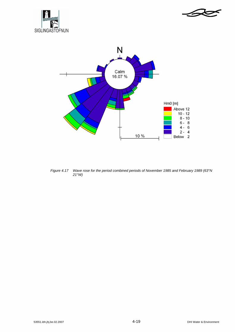
Figure 4.17 shows the wave climate when combining the two modelling periods of No-vember 1985 and February 1989 (see individual wave roses in Figure 2.1).
The offshore wave climate (63°N 21°W) for the period May 2006 to January 2007 is shown in Figure 4.16 and the measured morphology for May 2006 and January 2007 is given in Figure 4.18.
The wave climate in the period from May 2006 to January 2007 shows some resem-blance to the combined November 1985/February 1989 wave climate. During the com-bined period and the May-to-January period, wave-directions are dominated by south-westerly waves. Due to this similarity in the wave climates, the changes in the morphol-ogy from May 2006 to January 2007 and the changes modelled for the period Novem-ber 1985 and February 1989 can be expected to show similar patterns.
Changes in the outer bar morphology from May 2006 to January 2007 have taken place – see Figure 4.18. Both the pit-type trough and the outer bar are seen to have been eroded. During this period the outer bar is seen to have deepened 70 cm at the naviga-tion line intersection (i.e. ~9 cm/month). The morphological model predicted a deepen-ing in the order of ~10 cm/month at this location which is very close to the measured erosion rate (see Figure 4.18). The morphological changes are thus quite similar to the changes found with the numerical model. The model is seen to predict that the outer bar is subject to erosion during a wave climate that is comparable with that used in the modelling periods.
Figure 4.16 Wave rose for the period May 2006 to January 2007 (63°N 21°W)
53551.ibh.jhj.be.02.2007 4-19 DHI Water & Environment
Figure 4.17 Wave rose for the period combined periods of November 1985 and February 1989 (63°N 21°W)

53551.ibh.jhj.be.02.2007 4-20 DHI Water & Environment
Figure 4.18 Measured bathymetry May 2006 (upper) and January 2007 (lower). The outer part of the breakwater is shown for reference

53551.ibh.jhj.be.02.2007 5-1 DHI Water & Environment
5 WAVES, CURRENTS AND BED LEVELS ALONG NAVIGATION LINE
In this section waves and flow along the navigation line are presented. Both the wave and current conditions are important for navigation. In addition, the simultaneous wave conditions at the Bakkafjara wave buoy and at two locations along the navigation line are investigated. The latter is important for the establishment of a transformation rule between waves measured at the buoy and waves along the navigation line.
5.1 Waves along the Navigation Line and at the Wave Buoy
The relation between the waves at the Bakkafjara wave buoy and the navigation line lo-cated in front of Bakkafjara Harbour is investigated by MIKE 21 SW. This was done to see if the transformation rule applied in the physical test facilities at Siglingastofnun could be verified by MIKE 21 SW. The location of the wave buoy (t3) and the naviga-tion line (t2 to t1) is shown in Figure 5.1.
Figure 5.1 Upper: location of wave buoy (t3) and navigation line (t1 to t2). Lower: depth along naviga-tion line [m]

53551.ibh.jhj.be.02.2007 5-2 DHI Water & Environment
MIKE 21 SW was set-up to calculate wave fields for both critical waves and 98% waves such that the wave height at the location of the wave buoy would give the wave condi-tions outlined in Table 5.1 and Table 5.2 (“critical waves” and “98% waves” are defined by Siglingastofnun). Wave heights in Table 5.1 and Table 5.2 are significant wave heights and tabulated as function of wave direction and surface elevation.
Table 5.1 Critical waves: significant wave heights at Bakkafjara wave buoy for different surface eleva-tions and wave directions
Surface elevation
Wave direction
Occurrence of direction
[%]
+2.3m +1.4m +0.5m 0.0m
South 22.5 3.8m/11s 3.7m/11s 3.5m/11s
South-west 51.7 3.9m/11s 3.8m/11s 3.5m/11s 3.4m/11s
South-east 25.8 3.8m/11s 3.6m/11s 3.5m/11s 3.4m/11s
Weighted 100 3.85m/11s 3.70m/11s 3.50/11s 3.40m/11s
Table 5.2 98% waves: significant wave heights and wave periods at Bakkafjara wave buoy for different surface elevations and wave directions
Surface elevation
Wave direction
+2.3m +1.4m +0.5m 0.0m
South 2.8m/7.6s 2.8m/7.6s 2.8m/7.6s
South-west 2.5m/8.8s 2.5m/8.8s 2.5m/8.8s 2.5m/8.8s
South-east 2.8m/6.8s 2.8m/6.8s 2.8m/6.8s 2.8m/6.8s
In Table 5.1 “weighted wave heights” are given as well. Weighted waves are found in the following way:
southeastssouthwestssouthsweighteds HSoutheastHSouthwestHSouthH ,,,, )%()%()%( ×+×+×=
where %() = occurrence of a wave from a given direction.
The waves are seen to vary nearly linearly with the surface elevation. Particularly, the variation of the weighted wave follows the following approximation:
WLH weighteds ×+= 2.04.3, /1/

53551.ibh.jhj.be.02.2007 5-3 DHI Water & Environment
where WL = surface elevation. The variation of the critical wave heights is shown in Figure 5.2 as function of the surface elevation for waves from south, south-west, south-east and the weighted waves (in grey). The approximation given in Eq /1/ is shown as well (in black).
Figure 5.2 Wave height (critical waves) with surface elevation for waves from south, south-west and south-east
As mentioned previously, MIKE 21 SW was set-up to calculate wave fields that match wave conditions at the Bakkafjara wave buoy (i.e. the waves in Table 5.1 and Table 5.2). This was done iteratively by first selecting typical wave events with wave directions from south, south-west and south-east and typical wave height distributions along the boundary of the model. The distribution of the wave height along the boundary of the model was scaled to give the wave heights in Table 5.1.
The wave heights calculated by MIKE 21 SW at the location of the Bakkafjara wave buoy were obtained with less than 3% discrepancy compared to those given in Table 5.1 and Table 5.2.
The wave model was run for 3 different spreading indexes, n, for all the cases given in Table 5.1. Directional spreading factors of n= 5, 10 and 20 were investigated (correspond-ing to the directional standard deviation of 23°, 17° and 12°, respectively). The modelled wave heights at 10 m and 6 m depth contour (along the navigation line) did not vary sig-nificantly with n; in fact results for n=10 and 20 differed by less than 3% when compared to n=5. Thus, the spreading factor is of much less importance than other factors in the wave modelling.
In Figure 5.3 is an example of the simulated waves for the case where waves are ap-proaching from south and the surface elevation is +2.3m. The plot includes information

53551.ibh.jhj.be.02.2007 5-4 DHI Water & Environment
on the position of the Bakkafjara wave buoy and the navigation line and contour lines in black show the water depth (water depth of May 2006). The figure is referred to as a Sea State Information Chart. The wave heights are seen to decrease in the alongshore direction. In Appendix C Sea State Information Charts for all cases given in Table 5.1 i.e. critical waves are presented. In Appendix D Sea State Information Charts for cases given in Table 5.1 i.e. 98% waves are presented.
Figure 5.3 Sea State Information Chart. Example of wave field for critical waves near the navigation line for water surface of +2.3 m and southern waves with indication of depth contours (shown with black lines). Indication of navigation line, extraction points and position of wave buoy (T3) is given
In Figure 5.4 the extracted wave heights along the navigation line (indication of extrac-tion line is given in Figure 5.1 and Figure 5.3) for scenarios given in Table 5.1 (critical waves) are presented.

53551.ibh.jhj.be.02.2007 5-5 DHI Water & Environment
Figure 5.4 Significant wave height [m] variation along the navigation line (see Figure 5.1) for different water depth with waves from south (scenarios given in Table 5.1 - critical waves). Surface elevations: black: +2.3m, green: +1.4m, red: +0.5m. Full drawn lines: numerical results
The variation in wave heights is seen to be influenced by shoaling and eventually wave breaking. The variation of the wave height through the surf zone is important for any coastal study; however, usually site-specific measurements or other information on how waves behave inside the surf zone are very limited. In this project, however, measure-ments are in fact available. The wave heights in the surf zone have been measured in a physical model established at the test facilities at Siglingastofnun. The model set-up and scale are described thoroughly in Ref. /2/. The measurements have been carried out for a range of surf elevations and directions at certain positions along the profile of the physical model bathymetry. Measurements are included in Figure 5.4 (red, green and black dots) and form an excellent opportunity for fine-tuning the wave-breaking model, see wave pa-rameters section.
Comparison between wave heights obtained from the numerical model (MIKE 21 SW) and the physical model (developed at physical test facilities at Siglingastofnun) along the navigation line is given in Appendix B for all wave directions (south, south-west and south east) and surface elevations. The numerical wave model is seen to capture the measured variation in wave height well taking into consideration that the physical model is using uni-directional waves and that the wave model does not consider wave reflection.
The wave heights from MIKE 21 SW at 10 m and 6 m water depth on the seaward fac-ing side of the bar (see Figure 5.1) are given in Table 5.3 for the wave conditions lined up in Table 5.1. The values are average values for different locations of the navigation line (average of 3 parallel navigation lines spaced approximately 25 m). This is done due to the significant variation in wave heights along the depth contour. Values pre-

53551.ibh.jhj.be.02.2007 5-6 DHI Water & Environment
sented in Table 5.3 are close to those obtained in the test facility of Siglingastofnun, see Ref. /2/, Table 1.
Table 5.3 Significant wave heights [m] at 10 m/6 m depth contour (CD) along the navigation line for dif-ferent surface elevations and wave directions. Water depth at crest of the bar is 6m CD
Surface elevation
Wave direction
+2.3m +1.4m +0.5m 0.0m
South 4.3m/4.1m 4.2m/3.9m 3.8m/3.5m
South-west 4.5m/4.1m 4.2m/3.8m 4.1m/3.4m 3.6m/3.3m
South-east 4.6m/4.3m 4.5m/4.0m 4.2m/3.6m 3.9m/3.0m
5.2 Currents along the Navigation Line
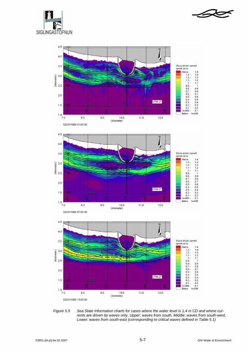
Figure 5.5 presents examples of Sea State Information Charts for wave driven currents with indication of the Bakkafjara wave buoy and the navigation line and contour lines in black show the water depth (water depths of May 2006). Examples correspond to cases defined in Table 5.1 (for water level of 1.4 m CD).
53551.ibh.jhj.be.02.2007 5-7 DHI Water & Environment
Figure 5.5 Sea State Information charts for cases where the water level is 1.4 m CD and where cur-rents are driven by waves only. Upper: waves from south, Middle: waves from south-west, Lower: waves from south-east (corresponding to critical waves defined in Table 5.1)
53551.ibh.jhj.be.02.2007 5-8 DHI Water & Environment
5.3 Waves along the Navigation Line during Selected Storms
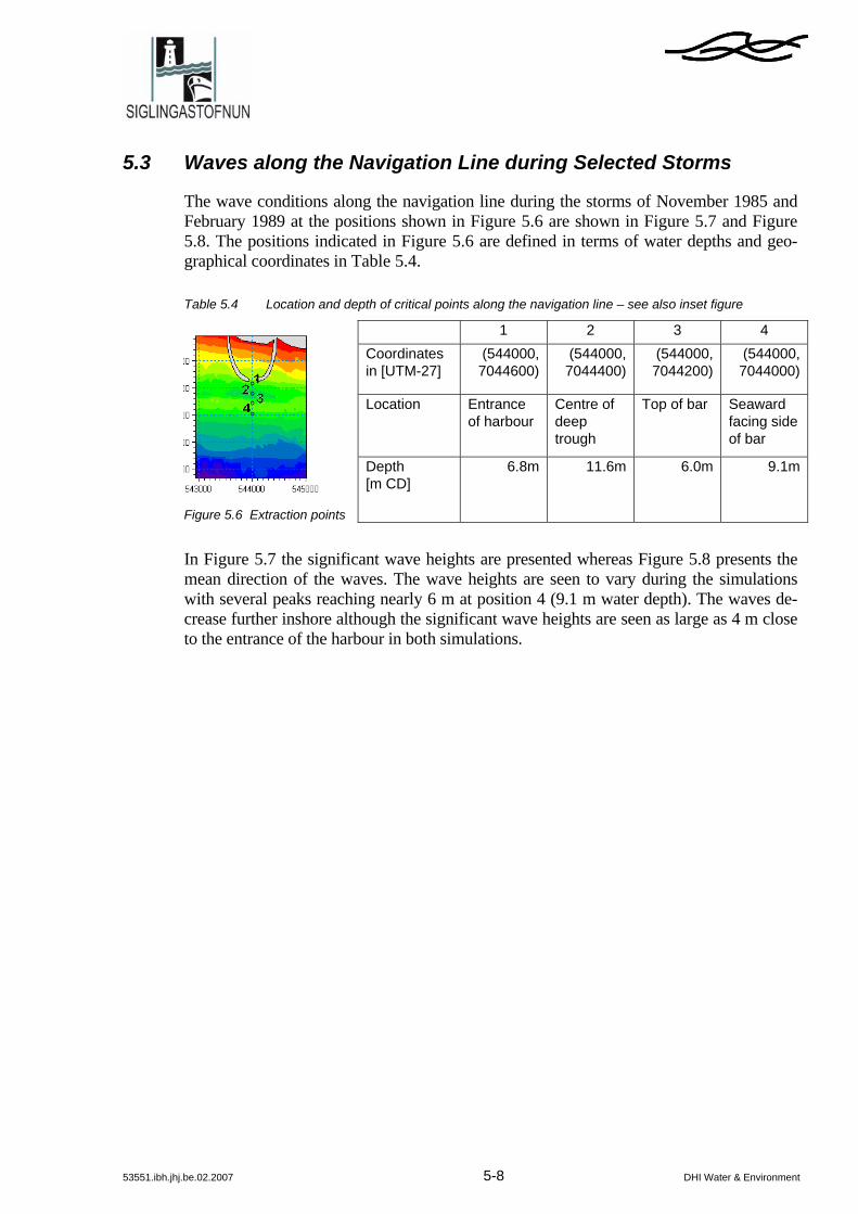
The wave conditions along the navigation line during the storms of November 1985 and February 1989 at the positions shown in Figure 5.6 are shown in Figure 5.7 and Figure 5.8. The positions indicated in Figure 5.6 are defined in terms of water depths and geo-graphical coordinates in Table 5.4.
Table 5.4 Location and depth of critical points along the navigation line – see also inset figure
1 2 3 4 Coordinates in [UTM-27]
(544000,7044600)
(544000, 7044400)
(544000,7044200)
(544000,7044000)
Location Entrance of harbour
Centre of deep trough
Top of bar Seaward facing side of bar
Figure 5.6 Extraction points
Depth [m CD]
6.8m 11.6m 6.0m 9.1m
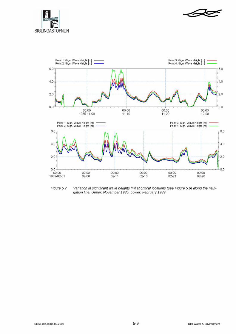
In Figure 5.7 the significant wave heights are presented whereas Figure 5.8 presents the mean direction of the waves. The wave heights are seen to vary during the simulations with several peaks reaching nearly 6 m at position 4 (9.1 m water depth). The waves de-crease further inshore although the significant wave heights are seen as large as 4 m close to the entrance of the harbour in both simulations.
53551.ibh.jhj.be.02.2007 5-9 DHI Water & Environment
Figure 5.7 Variation in significant wave heights [m] at critical locations (see Figure 5.6) along the navi-gation line. Upper: November 1985, Lower: February 1989
53551.ibh.jhj.be.02.2007 5-10 DHI Water & Environment
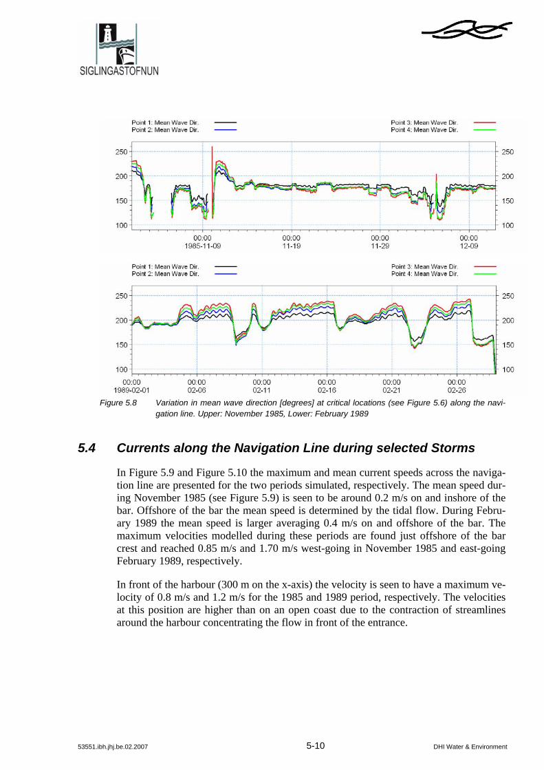
Figure 5.8 Variation in mean wave direction [degrees] at critical locations (see Figure 5.6) along the navi- gation line. Upper: November 1985, Lower: February 1989
5.4 Currents along the Navigation Line during selected Storms
In Figure 5.9 and Figure 5.10 the maximum and mean current speeds across the naviga-tion line are presented for the two periods simulated, respectively. The mean speed dur-ing November 1985 (see Figure 5.9) is seen to be around 0.2 m/s on and inshore of the bar. Offshore of the bar the mean speed is determined by the tidal flow. During Febru-ary 1989 the mean speed is larger averaging 0.4 m/s on and offshore of the bar. The maximum velocities modelled during these periods are found just offshore of the bar crest and reached 0.85 m/s and 1.70 m/s west-going in November 1985 and east-going February 1989, respectively.
In front of the harbour (300 m on the x-axis) the velocity is seen to have a maximum ve-locity of 0.8 m/s and 1.2 m/s for the 1985 and 1989 period, respectively. The velocities at this position are higher than on an open coast due to the contraction of streamlines around the harbour concentrating the flow in front of the entrance.

53551.ibh.jhj.be.02.2007 5-11 DHI Water & Environment
Figure 5.9 Maximum and mean current speeds [m/s] along the navigation line (perpendicular to the line) during November 1985
Figure 5.10 Maximum and mean current speeds [m/s] along the navigation line (perpendicular to the line) during February 1989
The current speeds during November/December 1985 and February 1989 at the positions indicated in Figure 5.6 are shown in Figure 5.11.
The calculated maximum velocities in the surf zone are sensitive to various set-up pa-rameters including the bed roughness and eddy viscosity. The bed roughness is introduced as a Manning Number and the eddy viscosity through a constant factor on the turbulence model. Applied values are central estimates based on experience from previous type pro-jects.

53551.ibh.jhj.be.02.2007 5-12 DHI Water & Environment
Figure 5.11 Variation in current speeds [m/s] at critical locations (see Figure 5.6) along the navigation line. Upper: November 1985, Lower: February 1989
5.5 Morphological Changes along Navigation Line
In Figure 5.12 the modelled bed level changes at the 4 locations shown in Figure 5.6 are shown. Not surprisingly, the morphological activity is seen to be pronounced during pe-riods of significant wave action. During the period of November 1985 the storm man-aged to modify the bathymetry especially on the bar. In the deep trough behind the bar (point 2) no changes were found; however, on the top of the bar (point 3) deposition of approximately 20 cm was found and slight erosion was seen on the sea facing side of the bar (point 4). Deposition in front of the harbour mouth was also seen (approximately 10 cm).
Generally, the changes in the navigation line are small in the period and are connected to the storms from 16-19 November. During the period of February 1989 no significant morphological activity was seen in the navigation line (fluctuation is less than 5 cm) ex-cept on the bar crest. The bar crest, however, was very mobile with an erosion of nearly 40 cm and a subsequent deposition of 50 cm.

53551.ibh.jhj.be.02.2007 5-13 DHI Water & Environment
Figure 5.12 Changes in bed level [m] at critical locations (see Figure 5.6) along the navigation line, No-vember 1985

53551.ibh.jhj.be.02.2007 5-14 DHI Water & Environment
Figure 5.13 Changes in bed level [m] at critical locations (see Figure 5.6) along the navigation line, Feb-ruary 1989
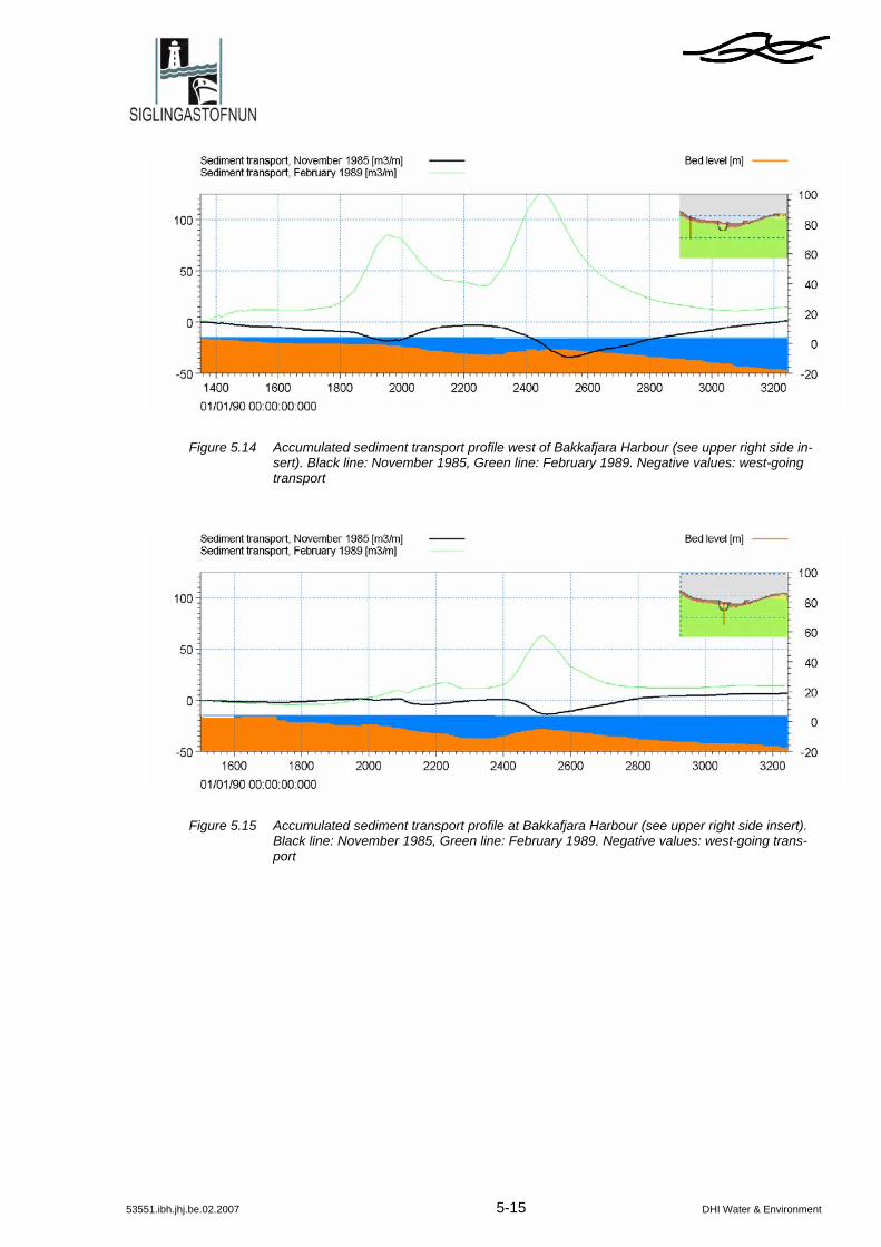
In Figure 5.14 and Figure 5.16 the longshore sediment transport profile west and east of Bakkafjara is depicted. The location of the profiles or cross-sections is indicated in the figure insert. The transport shows peaks in the transport rates near the crest of the bar; however, the results for the two periods are very different. During November 1985 (black line in the figures) the net transport west of Bakkafjara is to the west (negative values) whereas east of Bakkafjara the net transport was found to be eastward. At Bak-kafjara, Figure 5.15, the transport changes direction over the profile and is close to zero. This pattern is not seen for February 1989. Here the net transport was to the east in all cross-sections, although significantly smaller at Bakkafjara.
53551.ibh.jhj.be.02.2007 5-15 DHI Water & Environment
Figure 5.14 Accumulated sediment transport profile west of Bakkafjara Harbour (see upper right side in-sert). Black line: November 1985, Green line: February 1989. Negative values: west-going transport
Figure 5.15 Accumulated sediment transport profile at Bakkafjara Harbour (see upper right side insert). Black line: November 1985, Green line: February 1989. Negative values: west-going trans-port

53551.ibh.jhj.be.02.2007 5-16 DHI Water & Environment
Figure 5.16 Accumulated net sediment transport profile east of Bakkafjara Harbour (see upper right side insert). Black line: November 1985, Green line: February 1989. Negative values: west-going transport
In Table 5.5 the net integrated transports west, at and east of Bakkafjara are quantified for the two simulated periods. The transports show a clear tendency for an overall net eastward transport east of Bakkafjara.
Table 5.5 Integrated net transports west, at and east of Bakkafjara during the simulated periods
Period West of Bakkafjara At Bakkafjara East of Bakkafjara
November and half of December 1985 -38000 m3 -3800 m3 38200 m3
February 1989 117000 m3 38300 m3 102500 m3
5.6 Estimated Annual Transports
In Figure 2.3 the wave roses east and west of Bakkafjara for the modelled periods were compared to the annual wave climate. The comparison showed that the modelled peri-ods represent the annual wave climate well. This implies that the simulated periods are equally important.
The integrated net transports during the simulated periods may therefore be extended to annual transports by use of weights. By considering the percentage of time of each in-terval in the wave roses (i.e. for each of the coloured boxes in Figure 2.3) both for the annual, %Annual, and the modelled periods, %ModelPeriod, the following is obtained:
),(%%%1008
1
360
0MWDH sAnnual
HMWDCalms
s
∑∑==
+=

53551.ibh.jhj.be.02.2007 5-17 DHI Water & Environment
),(%%%1008
1
360
0MWDH sdModelPerio
HMWDCalms
s
∑∑==
+=
For each of the intervals (i.e. for each Hs, MWD) a net integrated sediment transport, Qs(Hs, MWD), can be calculated from the modelling results.
An assessment of the annual net integrated transport, Qs,Annual can therefore be made through the following extrapolation:
),(%
%8
1
360
0
MUDHQQ ssdModelPerio
Annual
HMWDAnnual
s
⋅= ∑∑==
Where .%
%conditionsofweight
dModelPerio
Annual =
The determination of the weights and the annual transport was calculated both west and east of Bakkafjara and the annual net transports were found to be 290,000 m3/year and 375,000 m3/year, respectively.
The transports east and west of Bakkafjara were calculated in Ref. /1/ and were found to be 400,000 m3/year and 300,000m3/year, respectively. The values estimated above are thus close to the values predicted with LITPACK in Ref. /1/.
Alternatively, if the selected storms are assumed to account for 3.5 months each (leav-ing 5 months to represent calm conditions with respect to inducing net drift), then the annual net transports estimated with MIKE 21 come close to the values estimated above and LITPACK results. (The weighting is shown in Table 5.6. In Ref. /1/ the LITPACK results showed (Figure 3.12 p. 3-12) a clear tendency for transport during late fall and winter months and less transport activity was found during late spring and summer month (5-6 months)).
Table 5.6 Integrated net transports west, at and east of Bakkafjara during the simulated periods
Period Weights [Months]
West of Bakkafjara [m3/month]
East of Bakkafjara [m3/month]
November 1985 3.5 -25.300 25.400 February 1989 3.5 117.000 102.500 Calm 5.0 0 0 Total 12 320.000 m3/yr 440.000 m3/yr
Using the weights given in Table 5.6, the annual net transport at Bakkafjara is estimated to 120,000m3/year. Again, this value agrees well with the calculated net transport at Bakkafjara reported in Ref. /1/. Here the net annual net transport was found to be ap-proximately 100,000m3/year (Figure 3.8 p. 3-8) in the period between 1979 and 2005.

53551.ibh.jhj.be.02.2007 5-18 DHI Water & Environment
The net integrated transports indicate that during November 1985 the morphology in the area around Bakkafjara suffered from net erosion. During February 1989 the total net morphological changes in the area were close to zero; however, local changes within the area (bounded by the three cross-sections) are seen with deposition to the west of the harbour and erosion to the east. This indicates that the bar and the depression in the bar moved to the east. Further, the river discharge pushes sand from the river mouth into the active littoral zone. This supply is expected to balance the losses when a longer time span is considered.
Since the work in Ref. /1/ was reported additional information on waves have become available. In Figure 5.17 the accumulated transport (net and gross) at Section 5 in the period between 2005 and 2006 is shown. In this period the net and gross transport were found to be 60,000 m3/year west-going and 300,000 m3/year, respectively, which is within the range of values found in preceding years (Table 3.11, Ref /4/) and well within the annual variability in transport rates and the conclusions drawn above are thus not altered.
.
Figure 5.17 Accumulated net (black line) and gross (blue and green lines added) transports in the period between 2005 and 2007 (a continuation of the calculations reported in Figure 3.11, Ref. /1/)

53551.ibh.jhj.be.02.2007 6-1 DHI Water & Environment
6 COASTAL IMPACT OF BAKKAFJARA PORT FACILITY
The coastline adjacent to the proposed Bakkafjara harbour will be affected by the har-bour due to its blockage of the littoral drift on the inner part of the profile. The long-term response of the harbour on the coastline is investigated in this section to supple-ment the shorter periods of morphological calculations presented previously and to pro-vide the following section dealing with sedimentation inside the harbour with input on the time scale of the coastline response.
The time required for the coastline to adapt fully to the new harbour from its original undisturbed state can be estimated roughly. To calculate the time it takes the accretion to reach the harbour entrance the following is assumed:
1 - Representative wave angle during storm from SW: 245° 2 - Present shoreline orientation 180° 3 - Extension of port from present shoreline: 600 m 4 - Active depth of the beach: 10 m 5 - Cross shore Extension of the port, W: 600 m The total volume of sand required for the fillet is estimated as:
Q = A×D where A = plan area (= 0.5×W×W/tan[245°-180°] ≈ 840000 m2) and D = active depth. Thus, the amount of sand necessary for the fillet is Q ≈ 840,000 m3. The annual drift landward of the outer bar and towards east is in the order of 120,000 m3/year. Thus a rough estimate of the time for the fillet to be established is approximately 7 years.
This is, however, an underestimation of the time scale as the coastline orientation will change continuously (rather than being constant as assumed in the rough estimation). To get a better estimate of the time scale the coastline evolution is taken into account by us-ing LITLINE which is part of LITPACK DHI’s software package for littoral drift and coastline kinetics. The LITLINE module simulates coastline evolution along a quasi-uniform coastline and calculates the coastline evolution by solving a continuity equation for the sediment in the littoral zone. The influence of structures, sources and sinks are included. LITLINE requires information on the sediment discharge from rivers, wave climates along the coastline stretch considered, the coastal profile and sediment proper-ties. This information is all available.
The model is set-up to calculate the coastline evolution starting from January 1989. The model takes the sediment load from Markarfljot into account by using the correlation between the river discharge from Ref. /3/ and the sediment load calculated with MIKE 21 FM (see Figure 3.10 and Figure 3.11). If this correlation is used the average annual sediment discharge is 150,000 m3/yr and the LITLINE model will maintain the delta at the 1989 level.

53551.ibh.jhj.be.02.2007 6-2 DHI Water & Environment
In the following, LITLINE results are presented.
In Figure 6.1 the coastline after 2 years (i.e. in January 1991) is shown both for the situation with (in white) and without (in dark military green) the proposed harbour. The total discharge of sand during this period is the same in both situations and amounts to 150,000m3/yr. Therefore, differences in the 1991-coastlines are related entirely to the presence of the harbour. It is seen that the proposed harbour will influence the coast near the breakwaters where sand is seen to accumulate on both sides of the breakwaters. The 1991-coastlines (with and without the harbour) are identical elsewhere also near the river delta implying that the river delta is almost not influenced by the harbour.
Figure 6.1 Coastline after 2 years with and without (dark green) the harbour. Simulation period: Janu-ary 1989 to January 1991 with sediment load from Markarfljot. White: accumulated material is in addition to natural evolution
In Figure 6.2 the coastline after 2 years (i.e. in January 1991) is presented both for a Markarfljot sediment discharge of 150,000 m3/yr (average annual discharge) and a dis-charge of 300,000 m3/yr (i.e. twice the average annual discharge). When the sediment discharge is doubled it is seen that the Markarfljot river delta expands and the additional sand being sourced into the coastal zone is seen to feed the coastline both east and west of the outlet. The delta expansion implies that the sediment transport capacity in the lit-toral zone in the vicinity of the Markarfljot river outlet is too small to remove the addi-tional sediment feed by the river. Still, the additional sediment discharge is not seen to affect the coastline near the harbour during the modelling period.

53551.ibh.jhj.be.02.2007 6-3 DHI Water & Environment
Figure 6.2 Coastline after 2 years for two different discharges. Simulation period: January 1989 to January 1991. White: accumulated material near the river
The optimal position of the harbour is investigated in the following for the simulation period: January 1989 to January 1991.
Figure 6.3 shows the coastline after 2 years (January 1991) in a situation where the po-sition of the harbour is located 500 m west of the proposed harbour and the discharge from Markarfljot is 150,000 m3/yr. The accretion in this case is seen to be larger than the accretion associated with the proposed position of the harbour (see Figure 6.1).

53551.ibh.jhj.be.02.2007 6-4 DHI Water & Environment
Figure 6.3 Initial coastline and coastline after 2 years for harbour located west of the proposed harbour Simulation period: January 1989 to January 1991. Yellow: accumulated material. Red: eroded material
Figure 6.4 shows the coastline after 2 years (January 1991) in a situation where the po-sition of the harbour is moved 500 m to the east of the proposed harbour and the dis-charge from Markarfljot is 150,000 m3/yr. Areas of accretion are shown with yellow.
The accretion of sand along the breakwaters is seen to be smaller than for the harbour located west of the proposed harbour. This is due to the more pronounced sheltering ef-fect of the Westmann Islands and the associated reduction in transport capacity. The ac-cretion along the breakwaters of the harbour located east of the proposed harbour is, however, similar to the accretion found for the proposed harbour itself (see Figure 6.1). It can thus be concluded that the location of the proposed harbour is close to an opti-mum as a certain distance from the Markafljot outlet is required. The mobility of the river outlet is great as demonstrated in Ref. /2/.

53551.ibh.jhj.be.02.2007 6-5 DHI Water & Environment
Figure 6.4 Initial coastline and coastline after 2 years for harbour located east of the proposed harbour Simulation period: January 1989 to January 1991. Yellow: accumulated material. Red: eroded material
In Figure 6.5 the coastline after 2, 5 and 10 years are presented. The simulations are car-ried out with the harbour located at the proposed location and with a fixed river mouth. The river sediment discharge is 150,000 m3/yr. The coastline at the river mouth is only modified slightly during the 10-year simulation period whereas the coastline in the vi-cinity of the breakwaters changes significantly and such that the coastline reaches the toe of the breakwaters after 10 years.

53551.ibh.jhj.be.02.2007 6-6 DHI Water & Environment
Figure 6.5 Initial coastline and coastline after 2, 5 and 10 years with harbour (fixed position of river out-let)
In the above, the final shape of the coastline near the harbour has been investigated with LITLINE. 2D effects around the harbour are taken into account through parameteriza-tion of certain processes. The importance of 2D effects can, however, be evaluated more directly by adopting the final coastline calculated with LITLINE in the MIKE 21 bathymetry i.e the bathymetry used by the 2D morphological model. The 2D model has been executed with this modified bathymetry and the coastline is seen to be adjusted. The applied modelling period is combined by the two selected simulation periods (Feb-ruary 1989 and November 1985) using a speed-up factor of 10. The combined period resembled the annual period – see Figure 2.3. In Figure 6.6 the equilibrium coastline ob-tained with LITLINE and MIKE 21 FM is shown. It is seen that LITLINE predicts lar-ger accumulation of sand near the breakwater. The acceleration of water along the breakwater, however, gives a smaller accretion here which entails a steepening of the profile. The process of profile steepening is not included in LITPACK.

53551.ibh.jhj.be.02.2007 6-7 DHI Water & Environment
Figure 6.6 Equilibrium coastline (after 10 years) at harbour with LITLINE (upper) and then modified in MIKE21FM (lower)

53551.ibh.jhj.be.02.2007 7-1 DHI Water & Environment
7 SEDIMENTATION INSIDE THE HARBOUR
In this section an assessment of the anticipated annual variability (or more technically: standard deviation) of the sedimentation and the mean annual sedimentation of the har-bour are carried out using the modelled sediment transport fields for the two periods se-lected and the coastline evolution presented in the previous section.
Figure 7.1 shows a snapshot of the sediment transport field around the entrance of the proposed Bakkafjara breakwaters just after its construction.
Figure 7.1 Calculated snap-shot sediment transport field around Bakkafjara breakwaters at the peak of
the February 1989 storm
As a rough estimate of the annual sedimentation into the harbour basin, the following rule of thumb for exchange of suspended sediment into a harbour basin can be applied (introduced in Ref. /1/):
WCVD 0.07 Q ×××=
where Q is the annual sedimentation (m3/year), D = water depth, V = current speed, C = mean concentration and W = width of the harbour entrance. The formula accounts for exchange of sediment due to the turbulence in the harbour entrance caused by the veloc-ity gradient. The velocity gradient is large as the velocity changes from the accelerated velocity just outside the harbour entrance to a value close to zero just inside the harbour.
To estimate annual sedimentation rates and to account for the impact of waves the for-mula has been interpreted in the following way:
1 W0.07 Q Q×= /1/
where Ql = longshore sediment transport (m3/m/year) passed the entrance.

53551.ibh.jhj.be.02.2007 7-2 DHI Water & Environment
In Ref. /1/ the sedimentation of the harbour was estimated to be in the order of 20,000 m3/year for a harbour with a 70 m wide entrance. This sedimentation rate was obtained with LITPACK by using the maximum gross transport rate on the inner part of the pro-file on the open coast. The sedimentation rate obtained by using the maximum gross sediment transport rate (in the inner part of the profile) corresponds to a value valid in the case where the morphology and coastline have attained its equilibrium profile around the breakwaters. The sedimentation rate is a central estimate based on 25 years of wave data. The variation in annual sedimentation (from year to year) will be evalu-ated as well.
The sedimentation rate valid just after the construction of the breakwaters can be esti-mated as well. According to LITDRIFT the initial sedimentation rates (from average wave conditions) can be estimated to be 1000-1500 m3/year. This value is obtained by considering Ql at a water depth of 5.5 m (from Figure 3.13 in Ref. /1/) which equals the smallest allowable water depth in the entrance of the harbour. This value can be com-pared to the sedimentation rates derived in the MIKE 21 FM model. The results from MIKE 21 FM are different from LITPACK results in the sense that they include 2D ef-fects. Thus, a better estimate of the sedimentation value is possible as both the effect of flow contraction and the effect of the 2D bathymetry on the wave conditions in front of the entrance are included.
Figure 7.2 presents the annual gross sediment transport profile in front of the harbour entrance estimated from the MIKE 21 FM results. The annual transport rates are ob-tained by utilizing the weights of modelled periods worked out previously – see Table 5.6. The gross annual transport profile, qgross,annual, can be estimated in one of the follow-ing ways:
CalmgrossNovembergrossFebruarygrossannualgross
sgrosssdModelPerio
Annual
HMWDannualgross
qqqq
MUDHqqs
,1985,1989,,
,
8
1
360
0,
0.55.35.3
),(%
%
×+×+×=
⋅= ∑∑==
where Qgross, February1989, Qgross, November1985 and Qgross, Calm given in Table 5.6 are the inte-grated values of qgross, February1989, qgross, November1985 and qgross, Calm.
Based on the results presented in Figure 7.2 the sedimentation rate is found to be ap-proximately 1300 m3/year and 1500 m3/year with these methods (using the maximum gross sediment transport rate in the profile just outside the 90 m wide entrance). This value is a little larger than that obtained with LITPACK (1000-1500m3/year) which can be attributed mainly to the contraction of streamlines around the breakwaters; a condi-tion which is disregarded in LITPACK. The 2D effects are thus responsible for an in-crease in sedimentation. Based on the analysis presented above, the increase due to 2D effects is estimated to be approximately 25%. Having quantified the impact of 2D ef-fects, an assessment of the annual sedimentation in the case of a fully developed mor-phology can be derived. Due to the influence of 2D effects the annual sedimentation in the fully developed situation is estimated to be 25,000 m3/year for a 70 m wide en-trance.

53551.ibh.jhj.be.02.2007 7-3 DHI Water & Environment
Figure 7.2 Estimated annual gross sediment transport profile in front of the harbour entrance. Profile is obtained by weighting calculated transport fields for the two periods modelled in MIKE 21 FM
The infill of sediment into the harbour from the 3D helical motion and sediment trans-ports induced by second order wave phenomena (wave asymmetry, streaming, wave drift) is not accounted for in the above estimate; however, the impact of these can be as-sessed by considering the period-averaged transport field in Figure 5.13 showing trans-ports normal to the depth-averaged flow direction. The order of magnitude of the trans-ports in Figure 5.13 is seen to be approximately 2-3 m3/m/year in the mouth of the breakwaters. The transports induced by these mechanisms thus contribute with ap-proximately 200-300 m3/year. The contribution is two orders of magnitude smaller than that caused by the turbulence of the main flow and can therefore be disregarded.
In Table 7.1 the sedimentation rates obtained with the two models are presented.
Table 7.1 Initial and equilibrium sedimentation rates estimated with LITPACK and MIKE 21 FM for three entrance widths
LITPACK (W=70m) Directly
MIKE 21 FM (W=70m) Weighted
MIKE 21 FM (W=90m) Weighted
MIKE 21 FM (W=110m) Weighted
Initial rates after construction [m3/year] 1,250 1,500 2,000 2,400 Equilibrium rates after construction [m3/year] 20,000 25,000 32,000 40,000

53551.ibh.jhj.be.02.2007 7-4 DHI Water & Environment
Recent refined assessments of the channel width suggest that an entrance width of approximately 86 m is sufficient. A channel width of 86 m entails a mean sedimentation rate after the coastline has adapted to the changes imposed by the harbour of 32,000 m3/year, which is 8,000 m3/year less than with a channel width of 110 m – see Table 7.1. The time required for the coastline to adapt from its original undisturbed state to a coastline that is in equilibrium with the har-bour is determined in Section 6 where the coastline evolution model is applied. The model shows that the transition from the undisturbed state is in the order of 10 years. In Table 7.2,
53551.ibh.jhj.be.02.2007 7-5 DHI Water & Environment
Table 7.3 and
Table 7.4 sedimentation rates during these 10 years of transition are given for entrance widths of 70 m, 90 m and 110 m, respectively.
Annual sedimentation rates presented so far are mean values. The sedimentation rate is, however, expected to vary from year to year due to its strong dependency on the wave climate. In Ref. /1/, Figure 3.11 the annual gross longshore transport at Bakkafjara in the period from 1979 to 2005 can be found. As indicated in Eq. /1/ (shown above) the sedimentation is proportional to the gross longshore transport. Therefore, the variability in sedimentation can be estimated by considering the variability of the gross longshore transport from Figure 3.11. From Figure 3.11, Ref. /1/ the standard deviation in the annual gross transport can be determined. The standard deviation in the mean gross transport is found to be equal to half of the annual mean sedimentation rate. Thus, an upper and lower value for the an-nual sedimentation rate can be determined. These are presented in Table 7.2,
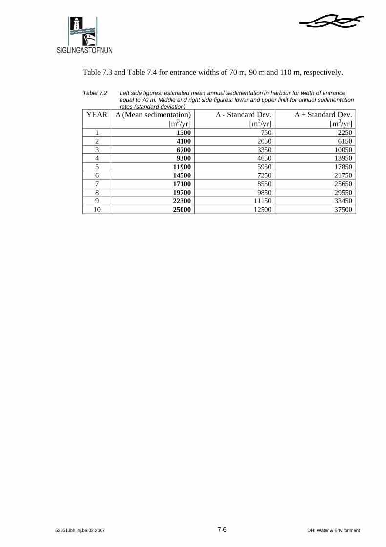
53551.ibh.jhj.be.02.2007 7-6 DHI Water & Environment
Table 7.3 and Table 7.4 for entrance widths of 70 m, 90 m and 110 m, respectively. Table 7.2 Left side figures: estimated mean annual sedimentation in harbour for width of entrance
equal to 70 m. Middle and right side figures: lower and upper limit for annual sedimentation rates (standard deviation)
YEAR
∆ (Mean sedimentation)[m3/yr]
∆ - Standard Dev.[m3/yr]
∆ + Standard Dev.[m3/yr]
1 1500 750 22502 4100 2050 61503 6700 3350 100504 9300 4650 139505 11900 5950 178506 14500 7250 217507 17100 8550 256508 19700 9850 295509 22300 11150 33450
10 25000 12500 37500

53551.ibh.jhj.be.02.2007 7-7 DHI Water & Environment
Table 7.3 Left side figures: estimated mean annual sedimentation in harbour for width of entrance equal to 90 m. Middle and right side figures: lower and upper limit for annual sedimentation rates (standard deviation)
YEAR ∆ (Mean sedimentation)
[m3/yr]∆ - Standard Dev.
[m3/yr]∆ + Standard Dev.
[m3/yr]1 2000 1000 30002 5300 2650 79503 8600 4300 129004 11900 5950 178505 15200 7600 228006 18500 9250 277507 21800 10900 327008 25100 12550 376509 28400 14200 42600
10 32000 16000 48000
Table 7.4 Left side figures: estimated mean annual sedimentation in harbour for width of entrance equal to 110 m. Middle and right side figures: lower and upper limit for annual sedimentation rates (standard deviation)
YEAR ∆ (Mean sedimentation)
[m3/yr]∆ - Standard Dev.
[m3/yr]∆ + Standard Dev.
[m3/yr]1 2400 1200 36002 6550 3275 98253 10750 5375 161254 14950 7475 224255 19150 9575 287256 23350 11675 350257 27550 13775 413258 31750 15875 476259 35950 17975 53925
10 40000 20000 60000
The values presented in Table 7.2 to Table 7.4 are based on the fact that the coastline will be fully developed after 10 years. The variability in the development of the coast-line has not been considered in the sedimentation rate estimates. The fully developed coastline and sedimentation rates may thus be achieved after only 5 years or even 20 years (using the variability of the gross transport); however, the 10 years are a central estimate.
In Table 7.2 to Table 7.4 the amount of sediment captured by the harbour is presented. The sediment which is captured will settle where the water is calmer i.e. where veloci-ties are reduced. The sediment will thus mainly settle in the area just inside or between the breakwaters. Finer fractions of suspended material will settle along the inner side of the breakwaters i.e. further inside the harbour.
The sedimentation conditions just outside the entrance are treated in the following Sec-tion 8.
53551.ibh.jhj.be.02.2007 8-1 DHI Water & Environment
8 EQULIBRIUM WATER DEPTH IN FRONT OF HARBOUR ENTRANCE
In this section the water depths in front of the harbour entrance are considered.
A critical water depth of 5.5 m has been defined for the entrance area of the proposed Bakkafjara harbour. A requirement on entrance area water depths is defined to ensure that the ferry (connection Westmann Islands and the main land) will be able to navigate safely through the entrance. In the following the natural water depths in front of the en-trance will be investigated and an optimization of the configuration will be made to minimize sedimentation.
The natural or equilibrium water depths in front of the entrance are determined by the sediment transport capacity here. If the capacity is relatively large then sediment will be able to bypass at relatively large depths, whereas low transport capacities will result in relatively shallow depths.
The sediment transport capacity is determined by the level of turbulence near the seabed and in the water column. The turbulence is generated by the current and waves and acts as a stirring mechanism for keeping sediment in suspension. The transportation of the stirred sediment is caused by the current. In the present case the current plays an impor-tant role in the morphodynamics as the breakwater will concentrate the flow. The con-traction of the flow affects not only the sediment transport capacity but also how fast the sand is being removed. The interplay between the sediment transport capacity and the morphology is a highly non-linear process and the equilibrium morphology is a balance between complex processes. To determine such equilibrium the MIKE 21 FM model is applied using stationary offshore wave conditions to the point in time where equilibrium water depths are attained.
8.1 Stationary Conditions
So far the morphological model has been used to run historical periods, which include peaks as well as calms in the waves. Running historical events are important for the un-derstanding of the dynamics of the morphology and the dynamics of the bar during storms. The calculated changes in water depths in front of the harbour for the 1989 modelling period (with time factor 25) is shown in Figure 8.1. The location of the ex-traction points are shown in Figure 8.1 as well. The water depth in front of the harbour (point 2) changes from 9 m to 6.5 m during the period, with significant changes taking place during the peak of the storm. The adjustment of the water depth would have con-tinued if the duration of the storm was prolonged. In other words the duration of the storm is a governing factor for estimating the equilibrium depth. To better determine the potential water depths in front of the harbour the morphological model is executed by using stationary conditions.
In addition, the potential displacement of the bar depression is obtained.

53551.ibh.jhj.be.02.2007 8-2 DHI Water & Environment
Figure 8.1 Water depth at extraction points (upper part of figure) during the 1989 modelling period (us-ing time factor of 25)
The equilibrium water depths are investigated by considering the following (stationary) events (characteristic events are selected from the modelled simulation periods):
• Extreme south-westerly storm condition
• Moderate-to-rough south-westerly storm conditions
• Rough south-easterly storm condition
• Rough south-westerly storm conditions
In addition to these 4 stationary events, the rough south-westerly storm condition has been used to investigate the positive impacts of capital dredging on the water depths. The water depths in front of the entrance are simulated using a bathymetry dredged to 7 metres inside the harbour and in a confined area outside the entrance. Also, the angle

53551.ibh.jhj.be.02.2007 8-3 DHI Water & Environment
between the orientation of the outer part of the breakwaters have been investigated to optimize the configuration with respect to minimizing sedimentation.
The selected conditions are representative for the rough wave climate. The morphologi-cal model is executed to a point where a bar along the up-drift side of the breakwaters has developed and where water depths in the area in front of the entrance have attained the value of equilibrium. To reach this stage a speed-up factor of 10 on the morphologi-cal development has been applied.
The wave fields for the 6 different cases are shown in Figure 8.2 to Figure 8.7 for the initial bathymetry.
Figure 8.2 Rough south-easterly condition (st-1985)
Figure 8.3 Moderate-to-rough south-westerly condition (st-1985-navdepth-peak2)

53551.ibh.jhj.be.02.2007 8-4 DHI Water & Environment
Figure 8.4 Extreme south-westerly condition (st-1985-navdepth-peak)
Figure 8.5 Rough south-westerly condition (st-1985-4)
Figure 8.6 Rough south-westerly condition. Capital dredging inside and around the breakwaters (st-5b)

53551.ibh.jhj.be.02.2007 8-5 DHI Water & Environment
Figure 8.7 Rough south-westerly condition. Larger angle between the orientation of breakwaters (gle)
Further, the wave cases presented in Figure 8.2 to Figure 8.7 are listed in Table 8.1 in terms of the significant wave heights at the Bakkafjara wave buoy.
Table 8.1 Wave heights at wave buoy for wave conditions shown in Figure 8.2 to Figure 8.7.
Characterization of wave condition Wave heights at wave buoy [m]
Rough south-east 6.9
Moderate-to-rough south-west 2.7
Extreme south-west 5.0
Rough south-west 3.7
8.2 Morphological Evolution for Rough South-Westerly Conditions
In Figure 8.8 the morphological evolution for the rough south-westerly conditions are presented. On the up-drift side of the harbour along the breakwater a bar is seen to form. The bar is seen to migrate towards the entrance, however only to a certain point. The bar growth ceases when an equilibrium between the sediment transport capacity and the wa-ter depth is attained.
The final bathymetry shown in Figure 8.8 with the outer bar and its attachment to the near-shore morphology east of the harbour resembles the bathymetry measured 7th May 2005. Prior to the May 2005 sounding significant storms from south-west were in fact observed.

53551.ibh.jhj.be.02.2007 8-6 DHI Water & Environment
Figure 8.8 Initial and final bathymetry (upper and middle). Close up of final bathymetry (lower). Rough south-westerly condition
The calculated change in water depths in front of the harbour for the rough south-westerly condition is shown in Figure 8.9. The water depth in front of the harbour (black line) is more than 6 m at the end of the calculation. The water depth of the outer bar near Bakkafjara is seen not to decrease during the simulation (stationary forcing).

53551.ibh.jhj.be.02.2007 8-7 DHI Water & Environment
Figure 8.9 Water depth at extraction points (see Figure 8.1) for rough south-westerly condition. (Hs=3.7m at Bakkafjara wave buoy)
The water depths in front of the entrance are calculated for other characteristic south-westerly conditions as well. Figure 8.10 presents water depths in front of the harbour for extreme conditions and mild-to-rough conditions. The water depth for the extreme con-dition reaches equilibrium quickly and at the end of the simulation the water depth was 7 m. In the mild-to-rough case water depths in front of the entrance were seen to be less than 5 m. Undulations in the water depth as function of time are pronounced for these cases and are due to the tidal flow.
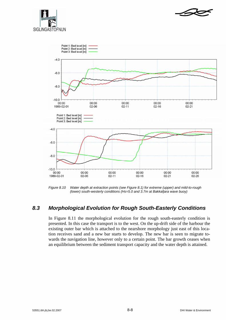
53551.ibh.jhj.be.02.2007 8-8 DHI Water & Environment
Figure 8.10 Water depth at extraction points (see Figure 8.1) for extreme (upper) and mild-to-rough (lower) south-westerly conditions (Hs=5.0 and 3.7m at Bakkafjara wave buoy)
8.3 Morphological Evolution for Rough South-Easterly Conditions
In Figure 8.11 the morphological evolution for the rough south-easterly condition is presented. In this case the transport is to the west. On the up-drift side of the harbour the existing outer bar which is attached to the nearshore morphology just east of this loca-tion receives sand and a new bar starts to develop. The new bar is seen to migrate to-wards the navigation line, however only to a certain point. The bar growth ceases when an equilibrium between the sediment transport capacity and the water depth is attained.

53551.ibh.jhj.be.02.2007 8-9 DHI Water & Environment
Figure 8.11 Initial and final bathymetry (upper and middle). Close up of final bathymetry (lower). Rough south-easterly condition
The final bathymetry shown in Figure 8.11 resembles the bathymetry measured in July 2004. Prior to the July 2004 sounding a very significant storm from south-east was ob-served.

53551.ibh.jhj.be.02.2007 8-10 DHI Water & Environment
The calculated change in water depth in front of the harbour for the rough south-easterly condition is shown in Figure 8.12. The water depth in front of the harbour (black line) is more than 8 m at the end of the calculation. The larger water depths found for south-easterly conditions compared to south-westerly conditions are due to the way sand is bypassing. In the case of south-westerly waves the sand is moving east along two main sediment routes; one is along the existing outer bar and one is along the inner part of the profile. The later route is eventually extended along the breakwater. The sand trans-ported along the breakwater is responsible for the development of the bar which mi-grates towards the harbour entrance. With south-easterly waves, on the other hand, the sand is moving west and because the existing outer bar is attached to the coastline just east of the harbour the sand will be bypassing along one main sediment route; the outer bar. As a consequence, the bar formation takes place more seaward for south-easterly waves and water depths are consequently larger.
Figure 8.12 Water depth at extraction points (see Figure 8.1) for rough south-easterly condition. (Hs=6.9m at Bakkafjara wave buoy)
8.4 Equilibrium Depth using Capital Dredging at Entrance
From the simulations of the morphological evolution presented above it was found that the bar developing on the up-drift side of the breakwater contains less sand than what is available in the existing bathymetry. The excess amount of sand in the existing bathym-etry bypasses the entrance in the initial stage just after the construction of the harbour. Once this excess amount of sand has bypassed or settled within the harbour entrance the morphology starts to adjust continuously towards equilibrium. During the passage of the excess sand water depths just outside the entrance area are seen to be smaller than the critical water depth of 5.5 m. Furthermore, sand is seen to be captured in the entrance it-self. As a consequence, water depths between the breakwaters remain below the critical threshold water depth of 5.5 m as the captured sand will not escape the sheltered en-trance. Outside the entrance the morphology will reach the same equilibrium as in the case of no capital dredging.
To reduce the amount of sand which is captured in the entrance a test is made where the bathymetry is dredged down to -7 m along the breakwaters and in the entrance area. This capital dredging situation is modelled for rough south-westerly conditions. In
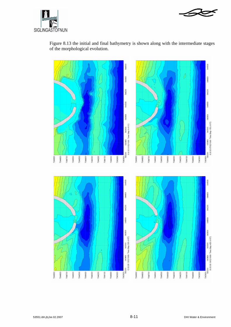
53551.ibh.jhj.be.02.2007 8-11 DHI Water & Environment
Figure 8.13 the initial and final bathymetry is shown along with the intermediate stages of the morphological evolution.

53551.ibh.jhj.be.02.2007 8-12 DHI Water & Environment
Figure 8.13 Close-up of initial bathymetry with capital dredging and intermediate stages of the bathymet-rical evolution (Hs=3.7m at Bakkafjara wave buoy)
Apart from the morphological changes near the entrance, the evolution presented in Figure 8.13 shows that the water depth at the outer bar does not change significantly in time. In fact, the water depths at the outer bar are seen to increase slightly at the position of the navigation line.
The changes in water depths in front of the harbour for the rough south-westerly condi-tion are shown in Figure 8.14. The water depth in front of the harbour (black line) is nearly 7 m at the end of the calculation.
Figure 8.14 Water depth at extraction points (see Figure 8.1) for rough south-westerly condition and capital dredging (Hs=3.7m at Bakkafjara wave buoy)

53551.ibh.jhj.be.02.2007 8-13 DHI Water & Environment
8.5 Equilibrium Depth for Different Breakwater Configurations
Sediment transport conditions in front of the entrance area are crucial for bypass and sedimentation. The transport of sediment around the harbour is determined by the stir-ring capacity of the flow and the ability of the current to transport the stirred material. Both factors can be controlled by the shape of the breakwaters. The shape of the break-waters should be streamlined such that the current is forced along the upstream break-water smoothly and such that the current is concentrated in front of the entrance area. One of the important parameters in the breakwater configuration is the shape of the outer part of the breakwater. Therefore, to meet the required navigation depth of 5.5 m the configuration of the outer part of the breakwaters has been investigated by altering the orientation of the outer part of the breakwaters. The orientation is measured as the angle between the orientation of the eastern and western breakwater heads. So far, the applied orientation has been 40° which is commonly accepted as an optimal angle with respect to minimizing sedimentation. However, the optimal angle may change under different conditions and environments. In the following, an angle of 65° is investigated.
In Figure 8.15 the final bathymetry for a breakwater orientation of 40° and 65° is shown. The final water depths in the case where the breakwaters have a 65° angle be-tween them are seen to be larger than with the 40°-case. The modification shows that an alteration of the angle has a positive impact on the water depths in front of the entrance.

53551.ibh.jhj.be.02.2007 8-14 DHI Water & Environment
Figure 8.15 Final bathymetries for an angle between the breakwaters of 40° (upper) and 65° (lower) de-grees (Hs=3.7m at Bakkafjara wave buoy)
The change in water depth in front of the harbour is shown in Figure 8.16. The initial water depths are larger in front of the entrance compared to the initial depths found with the 40° breakwaters as the breakwaters with the 65° angle extend a bit further seaward. At the end of the simulation, the water depth in front of the harbour (black line) is more than 7 m and close to an equilibrium value. The water depths are thus larger then the equilibrium water depths obtained with the 40° breakwaters. The increase in angle thus further improves the water depths in front of the entrance area.

53551.ibh.jhj.be.02.2007 8-15 DHI Water & Environment
Figure 8.16 Water depth at extraction points (see Figure 8.1) for rough south-westerly condition and an angle between the breakwaters of 65°. (Hs=3.7m at Bakkafjara wave buoy)
In Figure 8.17 the water depth at extraction points are shown for the rough south-easterly storm using an orientation of the breakwaters of 65°. The water depths are quite similar to the water depths found for an angle of 40°. The similar results are due to the fact that the sand is bypassing along the existing outer bar rather then building a secon-dary bar along the breakwater. Therefore, the details of the breakwater configuration are of less importance under these conditions.

53551.ibh.jhj.be.02.2007 8-16 DHI Water & Environment
Figure 8.17 Water depth at extraction points (see Figure 8.1) for rough south-easterly condition and an angle between the breakwaters of 65°. (Hs=6.9m at Bakkafjara wave buoy)
Finally, in Figure 8.18 the water depth at extraction points are shown for the mild-to-rough south-westerly storm using an orientation of the breakwaters of 65° with capital dredging. The water depth in the entrance area is close to 5.5 m.
Figure 8.18 Water depth at extraction points (see Figure 8.1) for mild-to-rough south-westerly condition and an angle between the breakwaters of 65° and with capital dredging. (Hs=2.7m at Bak-kafjara wave buoy)
8.6 Final Comments on the Equilibrium Water Depths
The water depth in front of the entrance has been assessed using the 2D morphological model. The depths have been investigated for different stationary wave conditions and the impact of capital dredging and the role of the angle between the breakwaters have been studied.
The harbour is found to perform well and to satisfy the minimum depth of 5.5 m outside the entrance area. The use of capital dredging gives less sedimentation problems inside the harbour and between the breakwaters. The capital dredging may, however, pose a breakwater stability problem. If capital dredging poses a stability problem, then addi-

53551.ibh.jhj.be.02.2007 8-17 DHI Water & Environment
tional maintenance dredging in the entrance area itself should be expected in the initial stage after the construction of the harbour (additional to that estimated in Section 7).
Furthermore, the angle between the breakwaters of 65° was seen to perform better than 40°.
The simulations of the morphology furthermore show that the pit-type feature and the depth over the outer bar at the navigation line are slightly modified and such that an in-crease in water depths compared to the initial bathymetry of May 2006 is found for all of stationary events considered. The pit-type feature is seen to migrate insignificantly and even deepen.
53551.ibh.jhj.be.02.2007 9-1 DHI Water & Environment
9 SUMMARY
9.1 Numerical Model
A coupled and fully integrated 2D numerical model for waves, currents and sediment transport (MIKE 21 FM) has been established to simulate impacts of a proposed har-bour on the morphological evolution of the surveyed May 2006 bathymetry both for sta-tionary forcing conditions and for historical periods. The later includes the two major storm periods: November 1985 and February 1989.
A validation of the wave model has been performed successfully. The wave model is seen to give excellent results capturing the significant wave height reduction from off-shore (south of Westmann Islands) to the wave buoy as well as the wave height attenua-tion in the surf-zone correctly. For the present investigation it is concluded that the near-shore wave climates are reproduced with sufficiently accuracy and further near-shore wave data (including directions) are presently not crucial for the studies.
In addition, the sediment transport model and the morphological model have been justi-fied. It so happens that the wave climate in the period from May 2006 to January 2007 resembles the combined modelling periods of November 1985 and February 1989. A bathymetric survey in the area around the navigation line was undertaken both in May 2006 and in January 2007 and the erosion/deposition pattern is therefore available for this period. During this period the bar deepened 70 cm. The morphological model pre-dicted a deepening of 10 cm/month which is very close to the measured erosion rate.
9.2 Configuration of Harbour
The proposed harbour is composed by two breakwaters. The proposed entrance width is 90 m and the initial water depth (May 2006 Bathymetry) here is 8 m. The location of the harbour has been investigated both with LITLINE and a very detailed morphological model and the proposed position is found to be optimal. The water depths in the en-trance area were investigated using the MIKE 21 FM and stationary forcing conditions to obtain the potential depths for various storm scenarios. The morphological calcula-tions show that if an angle between the breakwaters of 65° is used then a water depth of 5.5 m in front of the harbour entrance can be maintained. Thus, the alignment of the outer part of the eastern and western breakwater is such that the angle between them should be 65°.
9.3 Sedimentation of Harbour
The determination of the equilibrium depths in front of the entrance with MIKE 21 FM revealed that the use of capital dredging would decrease the sedimentation problems in the entrance area. This is because more sand is present in the existing profile than in the equilibrium profile found after the construction of the harbour. Obviously, a fraction of this excess amount of sand is seen to settle between and within the breakwaters. The use
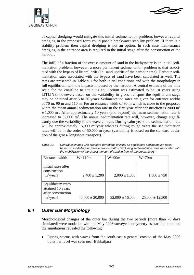
53551.ibh.jhj.be.02.2007 9-2 DHI Water & Environment
of capital dredging would mitigate this initial sedimentation problem; however, capital dredging in the proposed form could pose a breakwater stability problem. If there is a stability problem then capital dredging is not an option. In such case maintenance dredging in the entrance area is required in the initial stage after the construction of the harbour.
The infill of a fraction of the excess amount of sand in the bathymetry is an initial sedi-mentation problem; however, a more permanent sedimentation problem is that associ-ated with the bypass of littoral drift (i.e. sand updrift of the harbour area). Harbour sedi-mentation rates associated with the bypass of sand have been calculated as well. The rates are presented in Table 9.1 for both initial conditions and with the morphology in full equilibrium with the impacts imposed by the harbour. A central estimate of the time scale for the coastline to attain its equilibrium was estimated to be 10 years using LITLINE; however, based on the variability in gross transport the equilibrium stage may be obtained after 5 to 20 years. Sedimentation rates are given for entrance widths of 70 m, 90 m and 110 m. For an entrance width of 90 m which is close to the proposed width the mean annual sedimentation rate in the first year after construction is 2000 m3 ± 1,000 m3. After approximately 10 years (and beyond) the mean sedimentation rate is increased to 32,000 m3. The annual sedimentation rate will, however, change signifi-cantly due the variability in the wave climate. During calm years the sedimentation rate will be approximately 15,000 m3/year whereas during rough years the sedimentation rates will be in the order of 50,000 m3/year (variability is based on the standard devia-tion of the gross- longshore transport).
Table 9.1 Central estimates with standard deviations of initial an equilibrium sedimentation rates based on modelling for three entrance widths (excluding sedimentation rates associated with the mobilization of the excess amount of sand in front of the breakwaters)
Entrance width W=110m W=90m W=70m
Initial rates after construction [m3/year] 2,400 ± 1,200 2,000 ± 1,000 1,500 ± 750
Equilibrium rates attained 10 years after construction [m3/year] 40,000 ± 20,000 32,000 ± 16,000 25,000 ± 12,500
9.4 Outer Bar Morphology
Morphological changes of the outer bar during the two periods (more than 70 days simulated) were modelled with the May 2006 surveyed bathymetry as starting point and the simulations revealed the following:
• During storms with waves from the south-east a general erosion of the May 2006 outer bar level was seen near Bakkafjara

53551.ibh.jhj.be.02.2007 9-3 DHI Water & Environment
• During periods of south-westerly waves bed features were displaced eastward; how-ever, under these conditions a seaward deflection of the transport on the outer bar was found near Bakkafjara. A general (moderate) lowering of the May 2006 bar level was observed
• During periods of south-south-westerly waves the deflection of transport at the de-pression was seen to be more pronounced
Therefore, if the present bathymetry is exposed to conditions comparable with those of November 1985 and February 1989 the bar depression will not only be maintained but increased slightly. This points to the conclusion that the depression in the outer bar is maintained during storm periods comparable with those applied. This is a conclusion which is supported by the latest survey (January 2007) showing a significant lowering of the bar depression under forcing conditions (i.e. a wave climate) which is quite simi-lar to the forcing conditions applied in the numerical model.
To further understand the dynamics of the outer bar the following morphological modi-fications in the outer bar were made to the May 2006 bathymetry:
• Placing a pile of sand on the bar in front of the breakwaters • Excavating sand from the bar in front of the breakwaters
The modifications to the outer bar were made such that the water depth over the bar was reduced to 2 m over approximately 300 m in the alongshore direction and to 7 m over a distance of 150 m. In the former case, the storm was capable of eroding the pile of sand and the original level of the bar was nearly re-established. In the case of the excavated bar water depths in the central part of the excavation were increased by 10-20 cm over the period.
These findings fully support findings of previous simulations i.e. that the level of the bar in front of the deep pit-type trough is reduced under storm conditions. All simula-tions have demonstrated how two dominating morphodynamical mechanisms are at play during storm conditions. The resulting level of the bar is a continuous battle between the rip current induced scouring and the deposition of sand caused by the longshore current. In contrast to the shifting position of a rip channel on an open coast the position of the rip at Bakkafjara is locked to the zone in which the Westmann Islands provides shelter-ing. The Bakkafjara rip is thus more or less fixed and the existence of the bar depression is a robust morphological feature.
Having obtained an understanding of the importance of the rip current the extensive wave and bathymetrical data can be analysed with this in mind. The combination of great wave exposure west of Bakkafjara (which is a necessity for rip currents to be gen-erated) and relatively low rates of longshore transport at Bakkafjara are regarded as a prerequisite for the bar to deepen to the level seen in the May 2002 survey. By studying Table 2a through Table 3b in Ref. /1/ it is realised that this particular combination is not unusual. In fact, such combination can be identified in the tables in the years 1983, 1992, 1993 and 2001. On average the level seen in 2002 therefore has a probable return period of 8-10 years which is supported by the running average of the wave-energy from the offshore direction presented in Figure 4.14. The present level of the bar de-
53551.ibh.jhj.be.02.2007 9-4 DHI Water & Environment
pression is more likely to be the level characteristic for periods where the deposition caused by the longshore transport is counter-balanced by rip induced scouring. This level is not an exceptional level. The level of the bar depression was measured back in 1973 (the only survey of the bar conducted before 2002) to a similar level (5.8 m).
It is concluded that the bar formation at Bakkafjara is in a dynamic equilibrium with the forcing which has been present for the past decades. It may be critical for the develop-ment if significant changes in the dominant wave direction or the discharge of sediment due to globale climatic changes will take place. Such uncertainties have not been con-sidered.

53551.ibh.jhj.be.02.2007 10-1 DHI Water & Environment
10 REFERENCES
/1/ Bakkafjara. Sediment Transport and Morphology – Phase 1. By DHI for Siglingastofnun, January 2006.
/2/ Ferjuhöfn via Bakkafjöru. By Gísli Viggósson (Siglingastofnun), February 2006.
/3/ Markarfljót, calculated discharge with WaSiM-ETH watershed model. By ORKUSTOFNUN for Sinlinggastofnun, June 2006.
/4/ Ruessink, B.G., Walstra, D.J.R. and Southgate, H.N. 2003: Calibration and verification of a parametric wave model on barred beaches, Coastal Eng., 48, 139-149.

53551.ibh.jhj.be.02.2007 DHI Water & Environment
A P P E N D I X A
Morphological Changes of November 1985 and February 1989

53551.ibh.jhj.be.02.2007 DHI Water & Environment
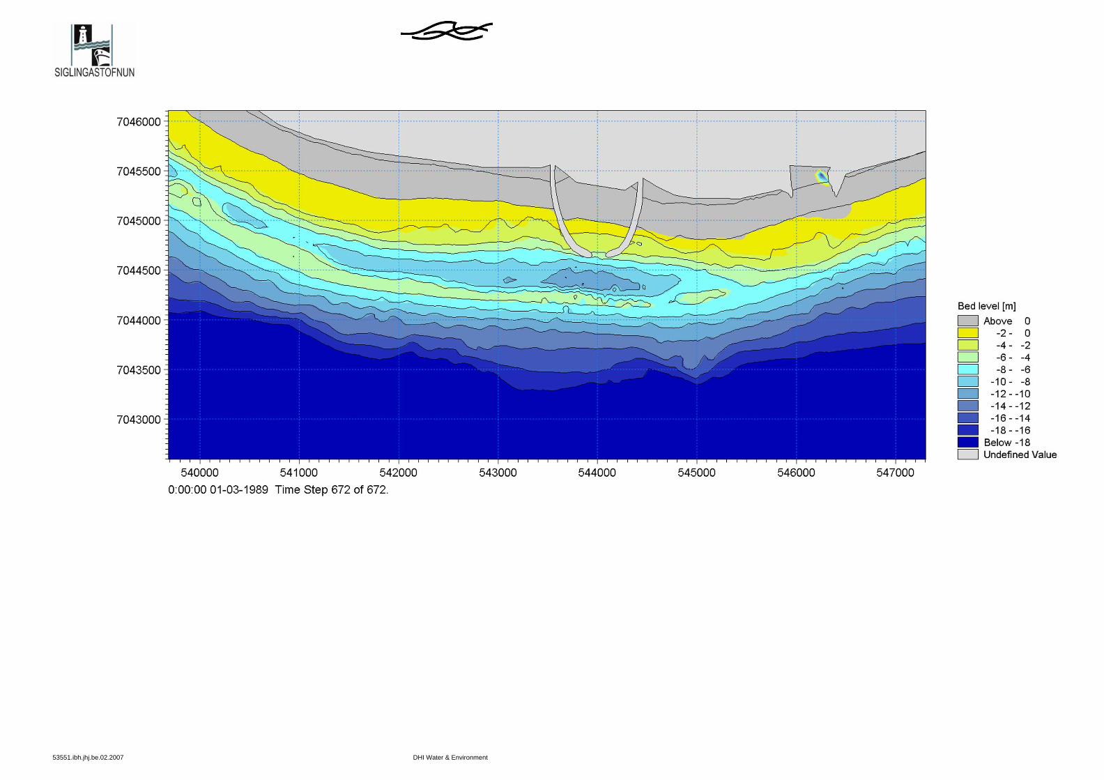
53551.ibh.jhj.be.02.2007 DHI Water & Environment

53551.ibh.jhj.be.02.2007 DHI Water & Environment
A P P E N D I X B
Comparison between Wave Heights along Navigation Line ob-tained in MIKE 21 SW and Physical Test Model

53551.ibh.jhj.be.02.2007 DHI Water & Environment
Wave-direction: SOUTH
Figure 10.1 Variation over bathymetry with 5.5m water depth (CD) at top of bar. Full drawn lines are nu-
merical model results
Figure 10.2 Variation over bathymetry with 6m water depth (CD) at top of bar. Full drawn lines are nu-
merical model results

53551.ibh.jhj.be.02.2007 DHI Water & Environment
Wave-direction: SOUTH-WEST
Figure 10.3 Variation over bathymetry with 5.5m water depth (CD) at top of bar. Full drawn lines are nu-
merical model results
Figure 10.4 Variation over bathymetry with 6m water depth (CD) at top of bar. Full drawn lines are nu-
merical model results

53551.ibh.jhj.be.02.2007 DHI Water & Environment
Wave-direction: SOUTH-EAST
Figure 10.5 Variation over bathymetry with 5.5m water depth (CD) at top of bar. Full drawn lines are nu-
merical model results
Figure 10.6 Variation over bathymetry with 6m water depth (CD) at top of bar. Full drawn lines are nu-
merical model results

53551.ibh.jhj.be.02.2007 DHI Water & Environment
A P P E N D I X C
Sea State Information Charts for Critical Waves
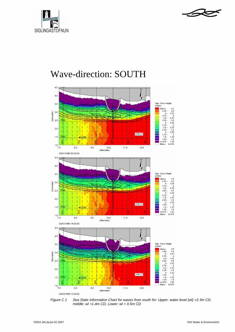
53551.ibh.jhj.be.02.2007 DHI Water & Environment
Wave-direction: SOUTH
Figure C.1 Sea State Information Chart for waves from south for: Upper: water level (wl) =2.3m CD,
middle: wl =1.4m CD, Lower: wl = 0.5m CD

53551.ibh.jhj.be.02.2007 DHI Water & Environment
Wave-direction: SOUTH-WEST
Figure C.2 Sea State Information Chart for waves from south-west for: Upper: water level (wl) =2.3m CD, middle: wl =1.4m CD, Lower: wl = 0.5m CD

53551.ibh.jhj.be.02.2007 DHI Water & Environment
Wave-direction: SOUTH-WEST cont’d
Figure C.3 Sea State Information Chart for waves from south-west for water level = 0.0m CD

53551.ibh.jhj.be.02.2007 DHI Water & Environment
Wave-direction: SOUTH-EAST
Figure C.4 Sea State Information Chart for waves from south-east for: Upper: water level (wl) =2.3m CD, middle: wl =1.4m CD, Lower: wl = 0.5m CD
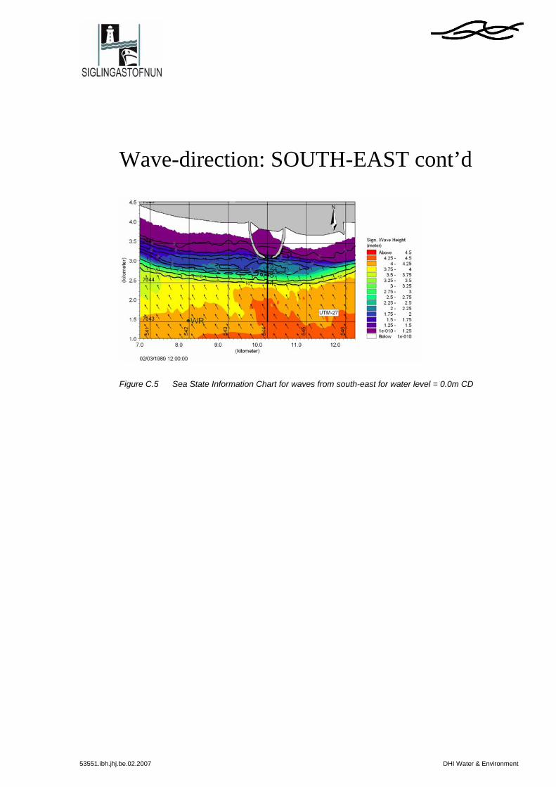
53551.ibh.jhj.be.02.2007 DHI Water & Environment
Wave-direction: SOUTH-EAST cont’d
Figure C.5 Sea State Information Chart for waves from south-east for water level = 0.0m CD

53551.ibh.jhj.be.02.2007 DHI Water & Environment
A P P E N D I X D
Sea State Information Charts for 98% Waves

53551.ibh.jhj.be.02.2007 DHI Water & Environment
Wave-direction: SOUTH
Figure D.3 Sea State Information Chart for waves from south for: Upper: water level (wl) =2.3m CD,
middle: wl =1.4m CD, Lower: wl = 0.5m CD

53551.ibh.jhj.be.02.2007 DHI Water & Environment
Wave-direction: SOUTH-WEST
Figure D.4 Sea State Information Chart for waves from south-west for: Upper: water level (wl) =2.3m CD, middle: wl =1.4m CD, Lower: wl = 0.5m CD

53551.ibh.jhj.be.02.2007 DHI Water & Environment
Wave-direction: SOUTH-WEST cont’d
Figure D.3 Sea State Information Chart for waves from south-west for water level = 0.0m CD
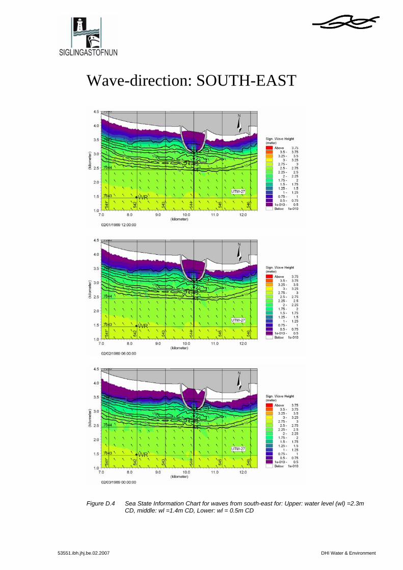
53551.ibh.jhj.be.02.2007 DHI Water & Environment
Wave-direction: SOUTH-EAST
Figure D.4 Sea State Information Chart for waves from south-east for: Upper: water level (wl) =2.3m
CD, middle: wl =1.4m CD, Lower: wl = 0.5m CD

53551.ibh.jhj.be.02.2007 DHI Water & Environment
Wave-direction: SOUTH-EAST cont’d
Figure D.5 Sea State Information Chart for waves from south-east for water level = 0.0m CD