balance in the atmosphere: implications for numerical
TRANSCRIPT

Balance in the Atmosphere:Implications for Numerical Weather
Prediction
Peter LynchSchool of Mathematical Sciences
University College Dublin
BIRS Summer School, Banff, 10–15 July, 2011
Outline
Introduction to Initialization
Richardson’s Forecast
Scale Analysis of the SWE [Skip]
Early Initialization Methods
Laplace Tidal Equations [Skip]
Normal Mode Initialization
The Swinging Spring [Skip]
Digital Filter Initialization
Intro LFR Scales Early Methods LTE NNMI SS DFI
Outline
Introduction to Initialization
Richardson’s Forecast
Scale Analysis of the SWE [Skip]
Early Initialization Methods
Laplace Tidal Equations [Skip]
Normal Mode Initialization
The Swinging Spring [Skip]
Digital Filter Initialization
Intro LFR Scales Early Methods LTE NNMI SS DFI
Introduction to Initialization
I The spectrum of atmospheric motions is vast,encompassing phenomena having periodsranging from seconds to millennia.
I The motions of primary interest have relativelylong timescales.
I The mathematical models used for numericalprediction describe a broader span of dynamicalfeatures than those of direct concern.
Intro LFR Scales Early Methods LTE NNMI SS DFI

I For many purposes, the higher frequency (HF)components can be regarded as noise.
I The elimination of this noise is achieved byadjustment of the initial fields.
I This process is called initialization.
? ? ?
Intro LFR Scales Early Methods LTE NNMI SS DFI

Outline
Introduction to Initialization
Richardson’s Forecast
Scale Analysis of the SWE [Skip]
Early Initialization Methods
Laplace Tidal Equations [Skip]
Normal Mode Initialization
The Swinging Spring [Skip]
Digital Filter Initialization
Intro LFR Scales Early Methods LTE NNMI SS DFI

Richardson’s Forecast
I The story of Lewis Fry Richardson’s forecast iswell known.
I Richardson forecast the change in surfacepressure at a point in central Europe, using themathematical equations.
I His results implied a change in surface pressureof 145 hPa in 6 hours ! ! !
I As Sir Napier Shaw remarked, “the wildest guess. . . would not have been wider of the mark . . . ”.
Intro LFR Scales Early Methods LTE NNMI SS DFI

I Yet, Richardson claimed that his forecast was“. . . a fairly correct deduction from a somewhatunnatural initial distribution”.
I He ascribed the unrealistic value of pressuretendency to errors in the observed winds.
I This is only a partial explanation of the problem.
Intro LFR Scales Early Methods LTE NNMI SS DFI
The Spectrum of Atmospheric Motions
Atmospheric oscillations fall into two groups:I Rotational or vortical modes (RH waves)I Gravity-inertia wave oscillations
For typical conditions of large scale atmospheric flowthe two types of motion are clearly separated andinteractions between them are weak.
The high frequency gravity-inertia waves may belocally significant in the vicinity of steep orography,where there is strong thermal forcing or where veryrapid changes are occurring . . .. . . but overall they are of minor importance and maybe regarded as undesirable noise.
Intro LFR Scales Early Methods LTE NNMI SS DFI

Smooth Evolution of Pressure
Intro LFR Scales Early Methods LTE NNMI SS DFI

Noisy Evolution of Pressure
Intro LFR Scales Early Methods LTE NNMI SS DFI

Tendency of a Smooth Signal
Intro LFR Scales Early Methods LTE NNMI SS DFI

Tendency of a Noisy Signal
Intro LFR Scales Early Methods LTE NNMI SS DFI

A Richardsonian Limerick
Young Richardson wanted to knowHow quickly the pressure would grow.
But, what a surprise, ’cosThe six-hourly rise was,
In Pascals, One Four Five — Oh Oh!
Intro LFR Scales Early Methods LTE NNMI SS DFI
A Simple Example — Ocean Tides
Imagine that you are standing by the sea shore on astormy day.
The tidal variation, the slow changes between low andhigh water, has a period of about twelve hours.
Water level changes due to sea and swell haveperiods of less than a minute.
Clearly, the instantaneous value of water level cannotbe used for tidal analysis.
Intro LFR Scales Early Methods LTE NNMI SS DFI
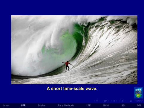
A short time-scale wave.
Intro LFR Scales Early Methods LTE NNMI SS DFI
At an instant, the water may be rising at a rate of onemetre per second.
If the vertical velocity observed at an instant is usedto predict the long-term movement of the water, anonsensical forecast is obtained:
Rise rate = 3,600 m/hr > 20 km in 6 hours
The instantaneous rate-of-change is no a guide to thelong-term evolution.
The same is true of the atmosphere!
Intro LFR Scales Early Methods LTE NNMI SS DFI

The Problem of Initialization.A subtle and delicate state of balance exists in theatmosphere between the wind and pressure fields.
The fast gravity waves have much smaller amplitudethan the slow rotational part of the flow.
The pressure and wind fields in regions not too nearthe equator are close to a state of geostrophicbalance and the flow is quasi-nondivergent.
The existence of this geostrophic balance is aperennial source of interest.
It is a consequence of the forcing mechanisms anddominant modes of hydrodynamic instability and ofthe manner in which energy is dispersed anddissipated in the atmosphere.
Intro LFR Scales Early Methods LTE NNMI SS DFI
When the primitive equations are used for numericalprediction the forecast may contain spurious largeamplitude high frequency oscillations.
These result from anomalously large gravity-inertiawave components, arising from in the observationsand analysis.
It was the presence of such imbalance in the initialfields that gave rise to the totally unrealistic pressuretendency of 145 hPa/6h obtained by Lewis FryRichardson.
The problems associated with high frequencymotions are overcome by the process known asinitialization.
Intro LFR Scales Early Methods LTE NNMI SS DFI

Evolution of surface pressure before and after NNMI.(Williamson and Temperton, 1981)
Intro LFR Scales Early Methods LTE NNMI SS DFI

Need for Initialization
The principal aim of initialization is to define theinitial fields so that the gravity inertia waves remainsmall throughout the forecast.
Specific requirements for initialization:
I Essential for satisfactory data assimilationI Noisy forecasts have unrealistic vertical velocityI Hopelessly inaccurate short-range rainfall
patternsI Spin-up of the humidity/water fields.I Imbalance can lead to numerical instabilities.
Intro LFR Scales Early Methods LTE NNMI SS DFI

Outline
Introduction to Initialization
Richardson’s Forecast
Scale Analysis of the SWE [Skip]
Early Initialization Methods
Laplace Tidal Equations [Skip]
Normal Mode Initialization
The Swinging Spring [Skip]
Digital Filter Initialization
Intro LFR Scales Early Methods LTE NNMI SS DFI

Scale-analysis of the SWE
A scale analysis of the SWE is detailed on thefollowing slides.
It will be omitted from the presentation, but isavailable for later study.
(Skip to next section.)
Intro LFR Scales Early Methods LTE NNMI SS DFI

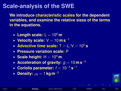
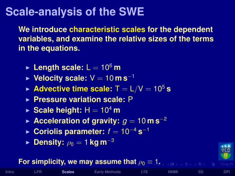
Scale-analysis of the SWEWe introduce characteristic scales for the dependentvariables, and examine the relative sizes of the termsin the equations.
I Length scale: L = 106 mI Velocity scale: V = 10 m s−1
I Advective time scale: T = L/V = 105 sI Pressure variation scale: PI Scale height: H = 104 mI Acceleration of gravity: g = 10 m s−2
I Coriolis parameter: f = 10−4 s−1
I Density: ρ0 = 1 kg m−3
For simplicity, we may assume that ρ0 ≡ 1.
Intro LFR Scales Early Methods LTE NNMI SS DFI
Scale-analysis of the SWEWe introduce characteristic scales for the dependentvariables, and examine the relative sizes of the termsin the equations.
I Length scale: L = 106 mI Velocity scale: V = 10 m s−1
I Advective time scale: T = L/V = 105 sI Pressure variation scale: PI Scale height: H = 104 mI Acceleration of gravity: g = 10 m s−2
I Coriolis parameter: f = 10−4 s−1
I Density: ρ0 = 1 kg m−3
For simplicity, we may assume that ρ0 ≡ 1.Intro LFR Scales Early Methods LTE NNMI SS DFI

The linear rotational shallow water equations are:∂u∂t︸︷︷︸
V2/L
− fv︸︷︷︸f V
+1ρ0
∂p∂x︸ ︷︷ ︸
P/L
= 0
∂v∂t︸︷︷︸
V2/L
+ fu︸︷︷︸f V
+1ρ0
∂p∂y︸ ︷︷ ︸
P/L
= 0
1ρ0
∂p∂t︸ ︷︷ ︸
PV/L
+ gH[∂u∂x
+∂v∂y
]︸ ︷︷ ︸
gHV/L
= 0
The scale of each term in the equations is indicated.
If there is approximate balance between the Coriolisand pressure gradient terms, we must have
PL
= fV or P = fLV = 103 Pa
Intro LFR Scales Early Methods LTE NNMI SS DFI
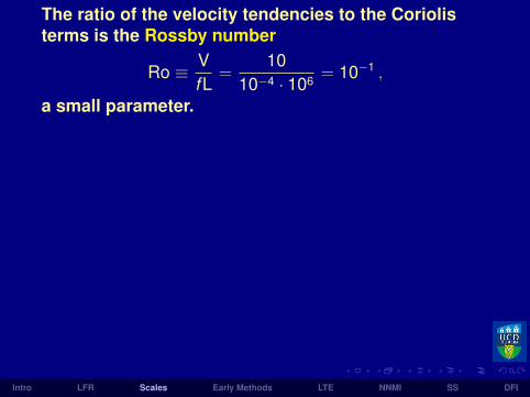
The ratio of the velocity tendencies to the Coriolisterms is the Rossby number
Ro ≡ VfL
=10
10−4 · 106 = 10−1 ,
a small parameter.
The scales of terms in the momentum equations are∂u∂t︸︷︷︸
10−4
− fv︸︷︷︸10−3
+1ρ0
∂p∂x︸ ︷︷ ︸
10−3
= 0
∂v∂t︸︷︷︸
10−4
+ fu︸︷︷︸10−3
+1ρ0
∂p∂y︸ ︷︷ ︸
10−3
= 0 .
To the lowest order of approximation, the tendencyterms are negligible; there is geostrophic balancebetween the Coriolis and pressure terms.
Intro LFR Scales Early Methods LTE NNMI SS DFI

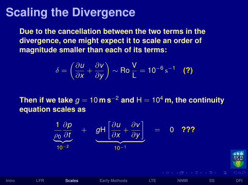
Scaling the DivergenceDue to the cancellation between the two terms in thedivergence, one might expect it to scale an order ofmagnitude smaller than each of its terms:
δ =
(∂u∂x
+∂v∂y
)∼ Ro
VL
= 10−6 s−1 (?)
Then if we take g = 10 m s−2 and H = 104 m, the continuityequation scales as
1ρ0
∂p∂t︸ ︷︷ ︸
10−2
+ gH[∂u∂x
+∂v∂y
]︸ ︷︷ ︸
10−1
= 0 ???
Impossible: there is nothing to balance the second term.
Intro LFR Scales Early Methods LTE NNMI SS DFI

Scaling the DivergenceDue to the cancellation between the two terms in thedivergence, one might expect it to scale an order ofmagnitude smaller than each of its terms:
δ =
(∂u∂x
+∂v∂y
)∼ Ro
VL
= 10−6 s−1 (?)
Then if we take g = 10 m s−2 and H = 104 m, the continuityequation scales as
1ρ0
∂p∂t︸ ︷︷ ︸
10−2
+ gH[∂u∂x
+∂v∂y
]︸ ︷︷ ︸
10−1
= 0 ???
Impossible: there is nothing to balance the second term.Intro LFR Scales Early Methods LTE NNMI SS DFI
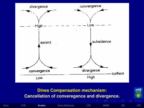
Dines Compensation mechanism:Cancellation of converegence and divergence.
Intro LFR Scales Early Methods LTE NNMI SS DFI
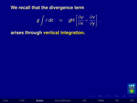
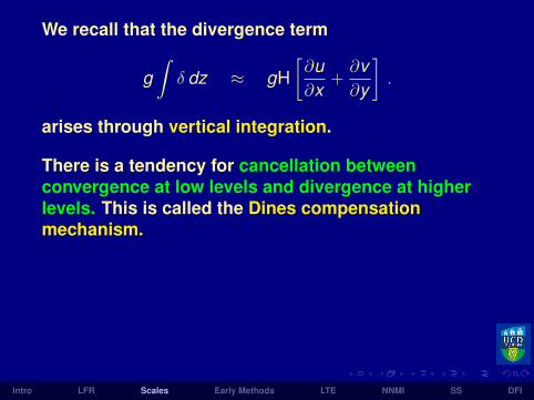
We recall that the divergence term
g∫δ dz ≈ gH
[∂u∂x
+∂v∂y
].
arises through vertical integration.
There is a tendency for cancellation betweenconvergence at low levels and divergence at higherlevels. This is called the Dines compensationmechanism.
Thus, we assume∫δ dz ∼ Ro δH , so that g
∫δ dz ∼ Ro2gH
VL
= 10−2 .
Intro LFR Scales Early Methods LTE NNMI SS DFI

The terms of the continuity equation are now inbalance:
1ρ0
∂p∂t︸ ︷︷ ︸
10−2
+ gH[∂u∂x
+∂v∂y
]︸ ︷︷ ︸
10−2
= 0
So, ∂p/∂t ∼ 10−2 Pa s−1, which is about 1 hPa per 3hours.
(Illustrate the Dines compensation mechanism for a cyclone.)
Intro LFR Scales Early Methods LTE NNMI SS DFI

The terms of the continuity equation are now inbalance:
1ρ0
∂p∂t︸ ︷︷ ︸
10−2
+ gH[∂u∂x
+∂v∂y
]︸ ︷︷ ︸
10−2
= 0
So, ∂p/∂t ∼ 10−2 Pa s−1, which is about 1 hPa per 3hours.
(Illustrate the Dines compensation mechanism for a cyclone.)
Intro LFR Scales Early Methods LTE NNMI SS DFI

The Effect of Data ErrorsSuppose there is a 10% error ∆v in the v -componentof the wind observation at a point.
The scales of the terms are as before:∂u∂t︸︷︷︸
10−4
− f (v + ∆v)︸ ︷︷ ︸10−3
+1ρ0
∂p∂x︸ ︷︷ ︸
10−3
= 0
However, the error in the tendency is∆(∂u/∂t) ∼ f ∆v ∼ 10−4, comparable in size to thetendency itself.
The signal-to-noise ratio is ∼1.
The forecast may be qualitatively reasonable, but itwill be quantitatively invalid.
Intro LFR Scales Early Methods LTE NNMI SS DFI

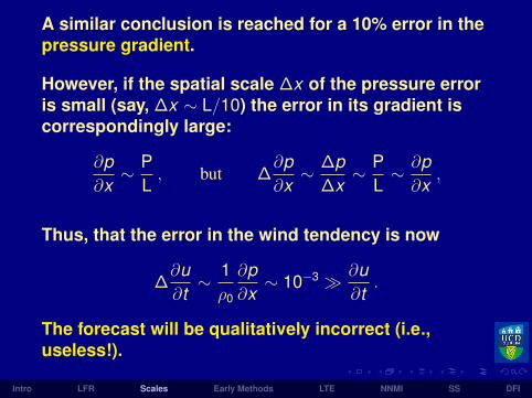
A similar conclusion is reached for a 10% error in thepressure gradient.
However, if the spatial scale ∆x of the pressure erroris small (say, ∆x ∼ L/10) the error in its gradient iscorrespondingly large:
∂p∂x∼ P
L, but ∆
∂p∂x∼ ∆p
∆x∼ P
L∼ ∂p∂x
,
Thus, that the error in the wind tendency is now
∆∂u∂t∼ 1ρ0
∂p∂x∼ 10−3 ∂u
∂t.
The forecast will be qualitatively incorrect (i.e.,useless!).
Intro LFR Scales Early Methods LTE NNMI SS DFI

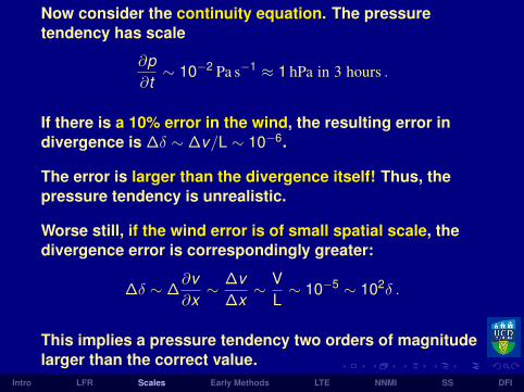
Now consider the continuity equation. The pressuretendency has scale
∂p∂t∼ 10−2 Pa s−1 ≈ 1 hPa in 3 hours .
If there is a 10% error in the wind, the resulting error indivergence is ∆δ ∼ ∆v/L ∼ 10−6.
The error is larger than the divergence itself! Thus, thepressure tendency is unrealistic.
Worse still, if the wind error is of small spatial scale, thedivergence error is correspondingly greater:
∆δ ∼ ∆∂v∂x∼ ∆v
∆x∼ V
L∼ 10−5 ∼ 102δ .
This implies a pressure tendency two orders of magnitudelarger than the correct value.
Intro LFR Scales Early Methods LTE NNMI SS DFI
Instead of the value ∂p/∂t ∼ 1 hPa in 3 hourswe get a change of order 100 hPa in 3 hours(like Richardson’s result).
Intro LFR Scales Early Methods LTE NNMI SS DFI

Evolution of surface pressure before and after NNMI.(Williamson and Temperton, 1981)
Intro LFR Scales Early Methods LTE NNMI SS DFI
Outline
Introduction to Initialization
Richardson’s Forecast
Scale Analysis of the SWE [Skip]
Early Initialization Methods
Laplace Tidal Equations [Skip]
Normal Mode Initialization
The Swinging Spring [Skip]
Digital Filter Initialization
Intro LFR Scales Early Methods LTE NNMI SS DFI
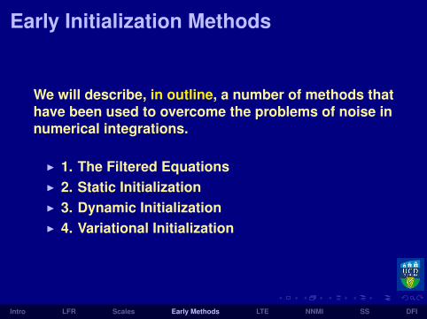
Early Initialization Methods
We will describe, in outline, a number of methods thathave been used to overcome the problems of noise innumerical integrations.
I 1. The Filtered EquationsI 2. Static InitializationI 3. Dynamic InitializationI 4. Variational Initialization
Intro LFR Scales Early Methods LTE NNMI SS DFI

1. The Filtered EquationsThe first computer forecast was made in 1950 byCharney, Fjørtoft and Von Neumann, using
ddt
(ζ + f ) = 0
which has no gravity wave components.
Systems like this are called Filtered Equations.The basic filtered system is the QG equations.
The barotropic, quasi-geostrophic potential vorticityequation (the QGPV Equation) is
∂
∂t(∇2ψ − Fψ
)+ J(ψ,∇2ψ) + β
∂ψ
∂x= 0 .
This is a single equation for a single variable, ψ.
Intro LFR Scales Early Methods LTE NNMI SS DFI

1. The Filtered EquationsThe first computer forecast was made in 1950 byCharney, Fjørtoft and Von Neumann, using
ddt
(ζ + f ) = 0
which has no gravity wave components.
Systems like this are called Filtered Equations.The basic filtered system is the QG equations.
The barotropic, quasi-geostrophic potential vorticityequation (the QGPV Equation) is
∂
∂t(∇2ψ − Fψ
)+ J(ψ,∇2ψ) + β
∂ψ
∂x= 0 .
This is a single equation for a single variable, ψ.Intro LFR Scales Early Methods LTE NNMI SS DFI
The simplifying assumptions have the effect ofeliminating high-frequency gravity wave solutions, sothat only the slow Rossby wave solutions remain.
? ? ?
A more accurate filtering of the primitive equationsleads to the balance equations.
This system is more complicated to solve than theQG system. It has not been widely used.
However one diagnostic component has been usedfor initialization. We discuss this presently.
Intro LFR Scales Early Methods LTE NNMI SS DFI

2. Static InitializationHinkelmann (1951) investigated the problem of noise innumerical integrations of the primitive equations.
He concluded that, if initial winds were geostrophic,
V =1f
k×∇Φ ,
HF oscillations would remain small in amplitude.
If we express the wind as V = k×∇ψ, we can write
f∇ψ = ∇Φ
The divergence of this is the linear balance equation:
∇·f∇ψ = ∇2Φ
This can be solved for ψ if Φ is given, or for Φ if ψ is given.
Intro LFR Scales Early Methods LTE NNMI SS DFI

2. Static InitializationHinkelmann (1951) investigated the problem of noise innumerical integrations of the primitive equations.
He concluded that, if initial winds were geostrophic,
V =1f
k×∇Φ ,
HF oscillations would remain small in amplitude.
If we express the wind as V = k×∇ψ, we can write
f∇ψ = ∇Φ
The divergence of this is the linear balance equation:
∇·f∇ψ = ∇2Φ
This can be solved for ψ if Φ is given, or for Φ if ψ is given.Intro LFR Scales Early Methods LTE NNMI SS DFI

Forecasts made with the primitive equations were soonshown to be clearly superior to those using thequasi-geostrophic system . . .. . . however, the use of geostrophic initial winds has ahuge disadvantage:
Observations of the wind field are completely ignored.
Charney (1955) proposed a better estimate of the wind,using the nonlinear balance equation.
This equation is a diagnostic relationship between thepressure and wind fields.
∇2Φ−∇·f∇ψ + 2
[(∂2ψ
∂x∂y
)2
− ∂2ψ
∂x2∂2ψ
∂y2
]= 0
This is a Poisson equation for Φ when ψ is given. However,it is nonlinear in ψ and hard to solve for ψ when Φ is given.
Intro LFR Scales Early Methods LTE NNMI SS DFI
When ψ is obtained from the nonlinear balanceequation, a non-divergent wind is constructed:
V = k×∇ψ .
Phillips (1960) argued that, in addition to getting ψfrom the nonlinear balance equation, a divergentcomponent of the wind should be included.
He proposed that a further improvement would resultif the divergence of the initial field were set equal tothat implied by quasi-geostrophic theory.
This can be sone by solving the QG omega equation.
Each of these steps represented some progress, butthe noise problem still remained essentially unsolved.
Intro LFR Scales Early Methods LTE NNMI SS DFI
3. Dynamic Initialization
Another approach, called dynamic initialization, usesthe forecast model itself to define the initial fields.
The dissipative processes in the model can damp outhigh frequency noise as the forecast procedes.
We integrate the model forward and backward in time,keeping the dissipation active all the time.
We repeat this forward-backward cycle many timesuntil we obtain initial fields from which the highfrequency components have been damped out.
Intro LFR Scales Early Methods LTE NNMI SS DFI

The forecast starting from the dynamically balancedfields is noise-free . . .
. . . however, the procedure is expensive in terms ofcomputer time.
Moreover, it damps the meteorologically significantmotions as well as the gravity waves.
Thus, dynamic initialization is no longer popular.
Intro LFR Scales Early Methods LTE NNMI SS DFI
3A. Digital filtering initialization (DFI)
Digital filtering initialization (DFI) is essentially arefinement of dynamic initialization.
Because it used a highly selective filtering technique,it is computationally more efficient than the olderdynamic initialization method.
If time permits, we will return to DFI later.
Intro LFR Scales Early Methods LTE NNMI SS DFI
4. Variational Initialization
An elegant initialization method based on thecalculus of variations was introduced by Sasaki(1958).
Although the method was not widely used, thevariational method is now at the centre of moderndata assimilation practice.
Recall that, in variational assimilation, we minimize acost function, J, which is normally a sum of two terms
J = JB + JO
Intro LFR Scales Early Methods LTE NNMI SS DFI
J(x) = JB(x) + JO(x)
Here, JB is the distance between the analysis and thebackground field
JB = 12(x− xb)T B−1(x− xb)
and JO is the distance to the observations
JO = 12 [yo − H(x)]T R−1[yo − H(xb)]
The idea is to choose x so as to minimize J(x).
? ? ?
The variational problem can be be modified to includea balance constraint.
Intro LFR Scales Early Methods LTE NNMI SS DFI

We add a constraint which requires the analysis to beclose to geostrophic balance:
JC = 12α∑
ij
[(fu + ∂Φ
∂y
)2
ij+(fv − ∂Φ
∂x
)2ij
]
This term JC is large if the analysis is far fromgeostrophic balance. It vanishes for perfectgeostrophic balance.
The weight α is chosen to give the constraint anappropriate impact. This is known as a weakconstraint.
The constrained variational assimilation finds theminimum of the cost function
J = JB + JO + JC
Intro LFR Scales Early Methods LTE NNMI SS DFI

Outline
Introduction to Initialization
Richardson’s Forecast
Scale Analysis of the SWE [Skip]
Early Initialization Methods
Laplace Tidal Equations [Skip]
Normal Mode Initialization
The Swinging Spring [Skip]
Digital Filter Initialization
Intro LFR Scales Early Methods LTE NNMI SS DFI

Atmospheric Normal Modes
The solutions of the atmospheric equations can beseparated, by spectral analysis, into two sets of linearnormal modes:
I Slow rotational components or Rossby modesI High frequency gravity-inertia modes
If the amplitude of the motion is small, the horizontalstructure is then governed by a system equivalent tothe linear shallow water equations.
These equations were first derived by Laplace in hisdiscussion of tides in the atmosphere and ocean.
They are called the Laplace Tidal Equations.
Intro LFR Scales Early Methods LTE NNMI SS DFI
The Laplace Tidal Equations
The simplest means of deriving the linear shallowwater equations from the primitive equations is toassume that the vertical velocity vanishes identically.
We assume that the motions can be described assmall perturbations about a state of rest, withconstant temperature T0, and pressure p(z) anddensity ρ(z) varying with height.
Intro LFR Scales Early Methods LTE NNMI SS DFI

The basic state variables satisfy the gas law, and arein hydrostatic balance:
p = RρT0 anddpdz
= −gρ
The variations of mean pressure and density follow:
p(z) = p0 exp(−z/H) , ρ(z) = ρ0 exp(−z/H) ,
where H = p0/gρ0 = RT0/g is the atmosphericscale-height.
Exercise: Confirm this.
Intro LFR Scales Early Methods LTE NNMI SS DFI

We consider only motions for which the verticalcomponent of velocity vanishes identically, w ≡ 0.
Let u, v , p and ρ denote variations about the basicstate, each of these being a small quantity. Then
∂ρu∂t− f ρv +
∂p∂x
= 0
∂ρv∂t
+ f ρu +∂p∂y
= 0
∂ρ
∂t+∇·ρV = 0
1γp
∂p∂t− 1ρ
∂ρ
∂t= 0
Density can be eliminated from the continuityequation by means of the thermodynamic equation.We then get three equations for u, v and p.
Intro LFR Scales Early Methods LTE NNMI SS DFI

We now assume that the horizontal and verticaldependencies of the perturbation quantities are separable:
ρuρvp
=
U(x , y , t)V (x , y , t)P(x , y , t)
Z (z) .
The momentum and continuity equations become∂U∂t− fV +
∂P∂x
= 0
∂V∂t
+ fU +∂P∂y
= 0
∂P∂t
+ (gh)∇ · V = 0
where V = (U,V ) is the momentum and h = γH = γRT0/g.
This is a set of three equations for U, V , and P.
They are mathematically isomorphic to the Laplace TidalEquations with a mean depth h (the equivalent depth).
Intro LFR Scales Early Methods LTE NNMI SS DFI

The Vertical Structure Equation
The vertical structure follows from the hydrostaticequation, together with the relationship p = (γgH)ρimplied by the thermodynamic equation. It isdetermined by
dZdz
+ZγH
= 0 ,
The solution of this is Z = Z0 exp(−z/γH), where Z0 isthe amplitude at z = 0.
Intro LFR Scales Early Methods LTE NNMI SS DFI

If we set Z0 = 1, then U, V and P give the momentumand pressure fields at the earth’s surface. Thesevariables all decay exponentially with height.
It follows that u and v actually increase with height asexp(κz/H), but the kinetic energy decays.
Solutions with more general vertical structures, andwith non-vanishing vertical velocity, may be derived.
Intro LFR Scales Early Methods LTE NNMI SS DFI

Vorticity and Divergence
We examine the solutions of the Laplace TidalEquations in some enlightening limiting cases.
By means of the Helmholtz Theorem, a generalhorizontal wind field V may be partitioned intorotational and divergent components
V = Vψ + Vχ = k×∇ψ +∇χ .
The stream function ψ and velocity potential χ arerelated to ζ and δ by the Poisson equations
∇2ψ = ζ and ∇2χ = δ .
Intro LFR Scales Early Methods LTE NNMI SS DFI

By differentiating the momentum equations, we getequations for the vorticity and divergence tendencies,e.g.,
∂ζ
∂t=
∂
∂t
(∂v∂x− ∂u∂y
)=
∂
∂x
(∂v∂t
)− ∂
∂y
(∂u∂t
)
Intro LFR Scales Early Methods LTE NNMI SS DFI

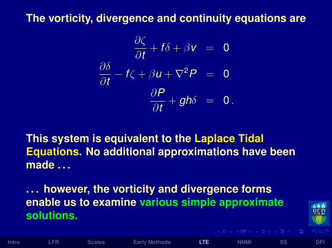
The vorticity, divergence and continuity equations are
∂ζ
∂t+ f δ + βv = 0
∂δ
∂t− f ζ + βu +∇2P = 0
∂P∂t
+ ghδ = 0 .
This system is equivalent to the Laplace TidalEquations. No additional approximations have beenmade . . .
. . . however, the vorticity and divergence formsenable us to examine various simple approximatesolutions.
Intro LFR Scales Early Methods LTE NNMI SS DFI

Mathematical Interlude
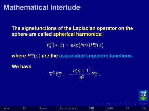
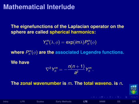
The eignefunctions of the Laplacian operator on thesphere are called spherical harmonics:
Y mn (λ, φ) = exp(imλ)Pm
n (φ)
where Pmn (φ) are the associated Legendre functions.
We have∇2Y m
n = −n(n + 1)
a2 Y mn .
The zonal wavenumber is m. The total waveno. is n.
Intro LFR Scales Early Methods LTE NNMI SS DFI
Mathematical Interlude
The eignefunctions of the Laplacian operator on thesphere are called spherical harmonics:
Y mn (λ, φ) = exp(imλ)Pm
n (φ)
where Pmn (φ) are the associated Legendre functions.
We have∇2Y m
n = −n(n + 1)
a2 Y mn .
The zonal wavenumber is m. The total waveno. is n.
Intro LFR Scales Early Methods LTE NNMI SS DFI

The ‘beta-term’ in the vorticity equation is
βv =2Ω cosφ
a
(1
a cosφ∂ψ
∂λ+
1a∂χ
∂λ
)
For quasi-non-divergent flow (|δ| |ζ|) it becomes
βv ≈ 2Ω
a2
∂ψ
∂λ
Intro LFR Scales Early Methods LTE NNMI SS DFI

The ‘beta-term’ in the vorticity equation is
βv =2Ω cosφ
a
(1
a cosφ∂ψ
∂λ+
1a∂χ
∂λ
)
For quasi-non-divergent flow (|δ| |ζ|) it becomes
βv ≈ 2Ω
a2
∂ψ
∂λ
Intro LFR Scales Early Methods LTE NNMI SS DFI

Rossby-Haurwitz ModesIf we suppose that the solution is quasi-nondivergent(that is, |δ| |ζ|), the wind is given approximately interms of the stream function (u, v) ≈ (−ψy , ψx ).
The vorticity equation becomes
∇2ψt + βψx = O(δ) ,
and we can ignore the right-hand side.
Assuming the stream function has the wave-likestructure of a spherical harmonic, we substitute
ψ = ψ0Y mn (λ, φ) exp(−iνt)
in the vorticity equation, and obtain the frequency:
ν = νR ≡ −2Ωm
n(n + 1).
Intro LFR Scales Early Methods LTE NNMI SS DFI
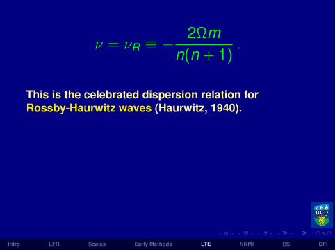
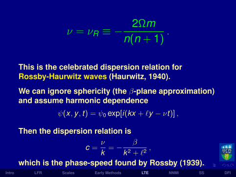
ν = νR ≡ −2Ωm
n(n + 1).
This is the celebrated dispersion relation forRossby-Haurwitz waves (Haurwitz, 1940).
We can ignore sphericity (the β-plane approximation)and assume harmonic dependence
ψ(x , y , t) = ψ0 exp[i(kx + `y − νt)] ,
Then the dispersion relation is
c =ν
k= − β
k2 + `2 ,
which is the phase-speed found by Rossby (1939).
Intro LFR Scales Early Methods LTE NNMI SS DFI
ν = νR ≡ −2Ωm
n(n + 1).
This is the celebrated dispersion relation forRossby-Haurwitz waves (Haurwitz, 1940).
We can ignore sphericity (the β-plane approximation)and assume harmonic dependence
ψ(x , y , t) = ψ0 exp[i(kx + `y − νt)] ,
Then the dispersion relation is
c =ν
k= − β
k2 + `2 ,
which is the phase-speed found by Rossby (1939).Intro LFR Scales Early Methods LTE NNMI SS DFI

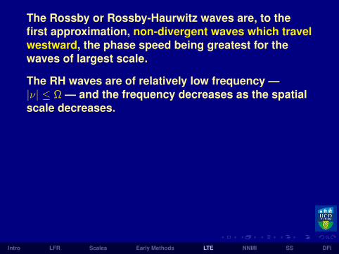
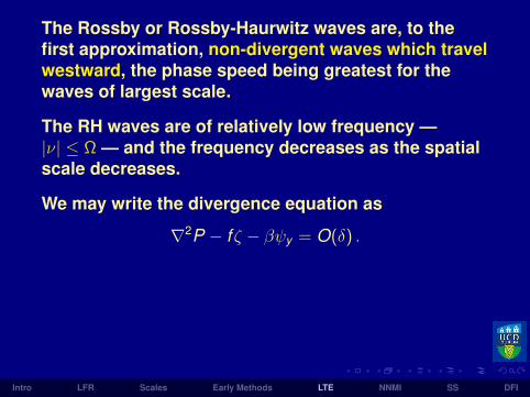
The Rossby or Rossby-Haurwitz waves are, to thefirst approximation, non-divergent waves which travelwestward, the phase speed being greatest for thewaves of largest scale.
The RH waves are of relatively low frequency —|ν| ≤ Ω — and the frequency decreases as the spatialscale decreases.
We may write the divergence equation as
∇2P − f ζ − βψy = O(δ) .
Ignoring the r.h.s., we get the linear balance equation
∇2P = ∇·f∇ψ ,
a diagnostic relationship between the geopotentialand the stream function.
Intro LFR Scales Early Methods LTE NNMI SS DFI
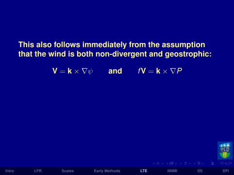
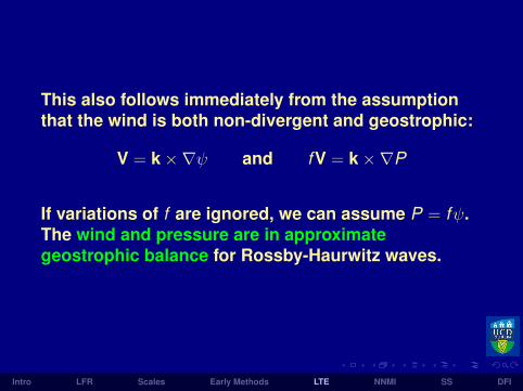
This also follows immediately from the assumptionthat the wind is both non-divergent and geostrophic:
V = k×∇ψ and fV = k×∇P
If variations of f are ignored, we can assume P = fψ.The wind and pressure are in approximategeostrophic balance for Rossby-Haurwitz waves.
Intro LFR Scales Early Methods LTE NNMI SS DFI
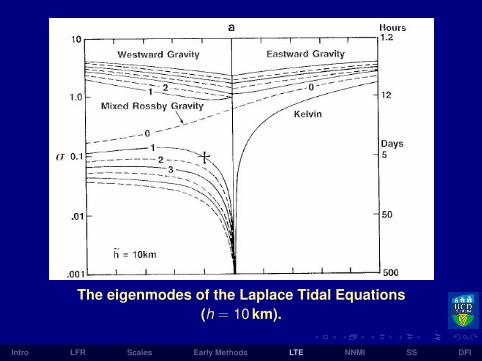
The eigenmodes of the Laplace Tidal Equations(h = 10 km).
Intro LFR Scales Early Methods LTE NNMI SS DFI

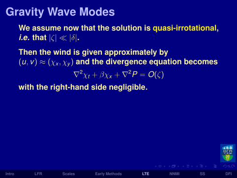
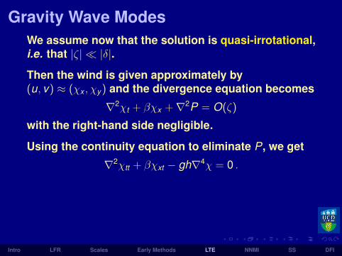
Gravity Wave ModesWe assume now that the solution is quasi-irrotational,i.e. that |ζ| |δ|.
Then the wind is given approximately by(u, v) ≈ (χx , χy ) and the divergence equation becomes
∇2χt + βχx +∇2P = O(ζ)
with the right-hand side negligible.
Using the continuity equation to eliminate P, we get
∇2χtt + βχxt − gh∇4χ = 0 .
If we look for a solution χ = χ0Y mn (λ, φ) exp(−iνt) we
find that
ν2 +
(− 2Ωm
n(n + 1)
)ν − n(n + 1)gh
a2 = 0 .
Intro LFR Scales Early Methods LTE NNMI SS DFI

ν2 +
(− 2Ωm
n(n + 1)
)ν − n(n + 1)gh
a2 = 0 .
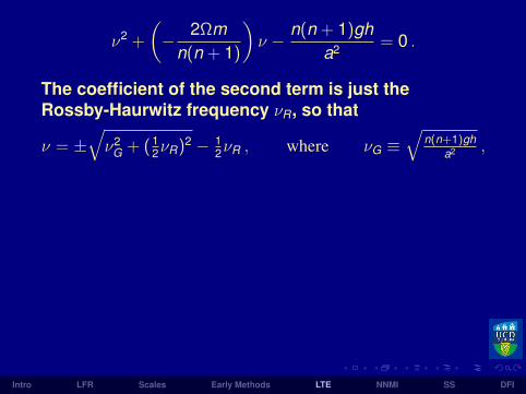
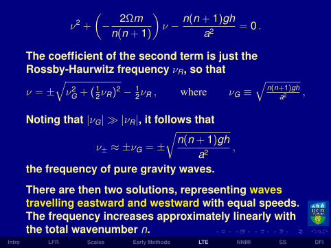
The coefficient of the second term is just theRossby-Haurwitz frequency νR, so that
ν = ±√ν2
G + (12νR)2 − 1
2νR , where νG ≡√
n(n+1)gha2 ,
Noting that |νG| |νR|, it follows that
ν± ≈ ±νG = ±√
n(n + 1)gha2 ,
the frequency of pure gravity waves.
There are then two solutions, representing wavestravelling eastward and westward with equal speeds.The frequency increases approximately linearly withthe total wavenumber n.
Intro LFR Scales Early Methods LTE NNMI SS DFI
ν2 +
(− 2Ωm
n(n + 1)
)ν − n(n + 1)gh
a2 = 0 .
The coefficient of the second term is just theRossby-Haurwitz frequency νR, so that
ν = ±√ν2
G + (12νR)2 − 1
2νR , where νG ≡√
n(n+1)gha2 ,
Noting that |νG| |νR|, it follows that
ν± ≈ ±νG = ±√
n(n + 1)gha2 ,
the frequency of pure gravity waves.
There are then two solutions, representing wavestravelling eastward and westward with equal speeds.The frequency increases approximately linearly withthe total wavenumber n.
Intro LFR Scales Early Methods LTE NNMI SS DFI

The eigenmodes of the Laplace TIdal Equations(h = 10 km).
Intro LFR Scales Early Methods LTE NNMI SS DFI

Outline
Introduction to Initialization
Richardson’s Forecast
Scale Analysis of the SWE [Skip]
Early Initialization Methods
Laplace Tidal Equations [Skip]
Normal Mode Initialization
The Swinging Spring [Skip]
Digital Filter Initialization
Intro LFR Scales Early Methods LTE NNMI SS DFI

Reminder on linear algebra
Let L be a matrix. An eigenvector e of L witheigenvalue λ satisfies
Le = λe
In general there are n eigenvectors for an n× n matrix.
We form the eigenvector and eigenvalue matrices
E = [e1,e2, . . . ,en] and Λ = diagλ1, λ2, . . . , λn
Intro LFR Scales Early Methods LTE NNMI SS DFI

Then the eigenvector relationships can be written as
LE = EΛ
For a symmetric matrix, the eigenvalues are real andthe eigenvectors are orthogonal:
EET = ETE = I .
It follows immediately that
L = EΛET and ETLE = Λ .
Intro LFR Scales Early Methods LTE NNMI SS DFI

Then the eigenvector relationships can be written as
LE = EΛ
For a symmetric matrix, the eigenvalues are real andthe eigenvectors are orthogonal:
EET = ETE = I .
It follows immediately that
L = EΛET and ETLE = Λ .
Intro LFR Scales Early Methods LTE NNMI SS DFI
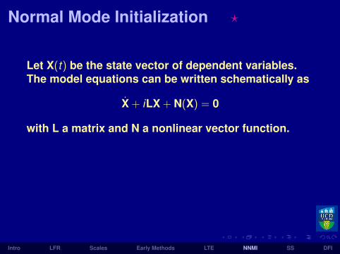
Normal Mode Initialization ?
Let X(t) be the state vector of dependent variables.The model equations can be written schematically as
X + iLX + N(X) = 0
with L a matrix and N a nonlinear vector function.
Denote the eigenvector matrix of L by E and thediagonal eigenvalue matrix as Λ. Then
ETLE = Λ .
Intro LFR Scales Early Methods LTE NNMI SS DFI

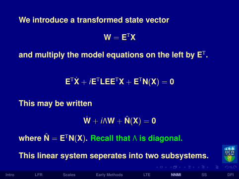
We introduce a transformed state vector
W = ETX
and multiply the model equations on the left by ET.
ETX + iETLEETX + ETN(X) = 0
This may be written
W + iΛW + N(X) = 0
where N = ETN(X). Recall that Λ is diagonal.
This linear system seperates into two subsystems.
Intro LFR Scales Early Methods LTE NNMI SS DFI

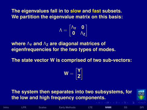
The eigenvalues fall in to slow and fast subsets.We partition the eigenvalue matrix on this basis:
Λ =
[ΛY 00 ΛZ
]where ΛY and ΛZ are diagonal matrices ofeigenfrequencies for the two types of modes.
The state vector W is comprised of two sub-vectors:
W =
[YZ
]
The system then separates into two subsystems, forthe low and high frequency components.
Intro LFR Scales Early Methods LTE NNMI SS DFI

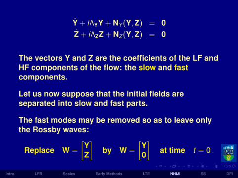
Y + iΛYY + NY (Y,Z) = 0Z + iΛZZ + NZ (Y,Z) = 0
The vectors Y and Z are the coefficients of the LF andHF components of the flow: the slow and fastcomponents.
Let us now suppose that the initial fields areseparated into slow and fast parts.
The fast modes may be removed so as to leave onlythe Rossby waves:
Replace W =
[YZ
]by W =
[Y0
]at time t = 0 .
Intro LFR Scales Early Methods LTE NNMI SS DFI
It might be hoped that this process of linear normalmode initialization, imposing the condition
LNMI: Z = 0 at t = 0would ensure a noise-free forecast.
However, the results are disappointing: the noise isreduced initially, but soon reappears.
The equations are nonlinear, and the slowcomponents interact nonlinearly in such a way as togenerate gravity waves.
The problem of noise remains: the gravity waves aresmall to begin with, but they grow rapidly.
Intro LFR Scales Early Methods LTE NNMI SS DFI

Surface pressure evolution: No Initialization and LNMI.
Intro LFR Scales Early Methods LTE NNMI SS DFI

To control the growth of HF components, BennertMachenhauer (1977) proposed setting their initialrate-of-change to zero, in the hope that they wouldremain small throughout the forecast.
Ferd Baer (1977) proposed a somewhat more generalmethod, using a two-timing perturbation technique.
The forecast, starting from initial fields modified sothat Z = 0 at t = 0 is very smooth and the spuriousgravity wave oscillations are almost completelyremoved.
Intro LFR Scales Early Methods LTE NNMI SS DFI

NNMI: Z = 0 at t = 0
Applying NNMI to the the equation for the fast modes:
Z + iΛZZ + NZ (Y,Z) = 0
we get
iΛZZ + NZ (Y,Z) = 0 or Z = iΛ−1Z NZ (Y,Z)
The method takes account of the nonlinear nature ofthe equations, and is referred to as nonlinear normalmode initialization.
Intro LFR Scales Early Methods LTE NNMI SS DFI

Surface pressure evolution: No Initialization and NNMI.
Intro LFR Scales Early Methods LTE NNMI SS DFI
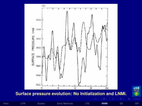
Surface pressure evolution: No Initialization and LNMI.
Intro LFR Scales Early Methods LTE NNMI SS DFI
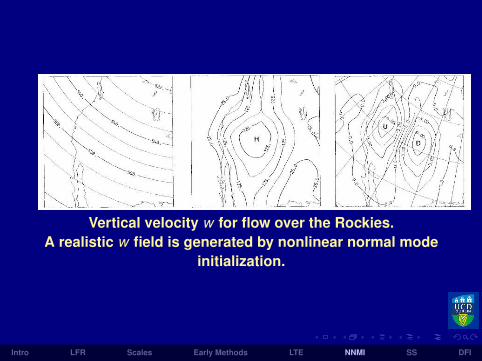
Vertical velocity w for flow over the Rockies.A realistic w field is generated by nonlinear normal mode
initialization.
Intro LFR Scales Early Methods LTE NNMI SS DFI
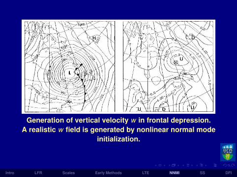
Generation of vertical velocity w in frontal depression.A realistic w field is generated by nonlinear normal mode
initialization.
Intro LFR Scales Early Methods LTE NNMI SS DFI

Outline
Introduction to Initialization
Richardson’s Forecast
Scale Analysis of the SWE [Skip]
Early Initialization Methods
Laplace Tidal Equations [Skip]
Normal Mode Initialization
The Swinging Spring [Skip]
Digital Filter Initialization
Intro LFR Scales Early Methods LTE NNMI SS DFI
Example: The Swinging Spring We will illustrate linear normal mode initialization(LNMI) and nonlinear normal mode initialization(NNMI) by application to a simple mechanical system.
The swinging spring comprises a heavy bobsuspended by a light elastic spring. The bob is free tomove in a vertical plane.
The oscillations of this system are of two types,distinguished by their restoring mechanisms.
We consider the elastic oscillations to be analoguesof the HF gravity waves in the atmosphere.
Similarly, the LF rotational motions correspond to therotational or Rossby waves.
Intro LFR Scales Early Methods LTE NNMI SS DFI
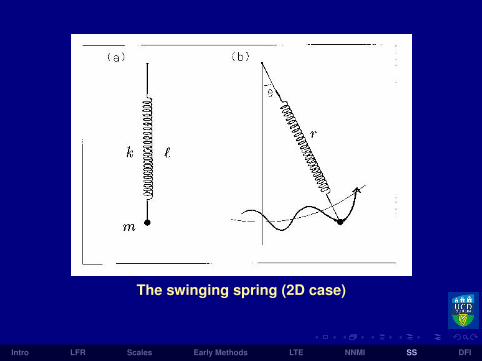
The swinging spring (2D case)
Intro LFR Scales Early Methods LTE NNMI SS DFI

The Dynamical EquationsLet `0 be the unstretched length of the spring, k itselasticity or stiffness and m the mass of the bob.
At equilibrium the balance of forces is:
k(`− `0) = mg
Polar coordinates qr = r and qθ = θ are used, and theradial and angular momenta are pr = mr , pθ = mr 2θ.
The Hamiltonian is (in this case) the sum of kinetic,elastic potential and gravitational potential energy:
H =1
2m
(p2
r +p2θ
r 2
)+ 1
2k(r − `0)2 −mgr cos θ .
Intro LFR Scales Early Methods LTE NNMI SS DFI
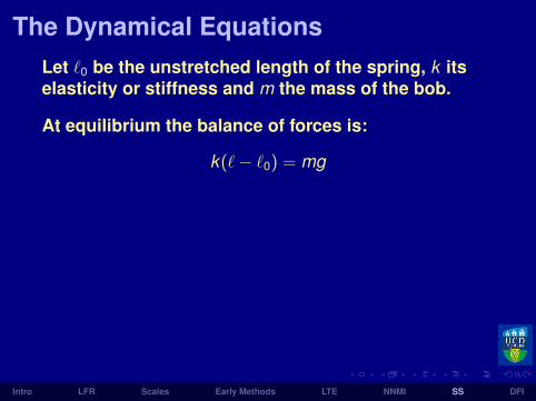
The Dynamical EquationsLet `0 be the unstretched length of the spring, k itselasticity or stiffness and m the mass of the bob.
At equilibrium the balance of forces is:
k(`− `0) = mg
Polar coordinates qr = r and qθ = θ are used, and theradial and angular momenta are pr = mr , pθ = mr 2θ.
The Hamiltonian is (in this case) the sum of kinetic,elastic potential and gravitational potential energy:
H =1
2m
(p2
r +p2θ
r 2
)+ 1
2k(r − `0)2 −mgr cos θ .
Intro LFR Scales Early Methods LTE NNMI SS DFI
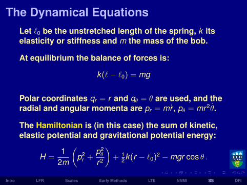
The Dynamical EquationsLet `0 be the unstretched length of the spring, k itselasticity or stiffness and m the mass of the bob.
At equilibrium the balance of forces is:
k(`− `0) = mg
Polar coordinates qr = r and qθ = θ are used, and theradial and angular momenta are pr = mr , pθ = mr 2θ.
The Hamiltonian is (in this case) the sum of kinetic,elastic potential and gravitational potential energy:
H =1
2m
(p2
r +p2θ
r 2
)+ 1
2k(r − `0)2 −mgr cos θ .
Intro LFR Scales Early Methods LTE NNMI SS DFI

The (canonical) dynamical equations are
θ = pθ/mr 2
pθ = −mgr sin θr = pr/m
pr = p2θ/mr 3 − k(r − `0) + mg cos θ .
These equations may be written symbolically as_X + LX + N(X) = 0
where X = (θ,pθ, r ,pr )T, L is the matrix for the linearterms and N is a nonlinear vector function.
We now suppose that the amplitude of the motion issmall, so that |r ′| = |r − `| ` and |θ| 1.
The state vector X comprises two sub-vectors:
X =
(YZ
), where Y =
(θpθ
)and Z =
(r ′
pr
).
Intro LFR Scales Early Methods LTE NNMI SS DFI

The (canonical) dynamical equations are
θ = pθ/mr 2
pθ = −mgr sin θr = pr/m
pr = p2θ/mr 3 − k(r − `0) + mg cos θ .
These equations may be written symbolically as_X + LX + N(X) = 0
where X = (θ, pθ, r ,pr )T, L is the matrix for the linearterms and N is a nonlinear vector function.
We now suppose that the amplitude of the motion issmall, so that |r ′| = |r − `| ` and |θ| 1.
The state vector X comprises two sub-vectors:
X =
(YZ
), where Y =
(θpθ
)and Z =
(r ′
pr
).
Intro LFR Scales Early Methods LTE NNMI SS DFI
We call the motion described by Y the rotationalcomponent and that described by Z the elasticcomponent.
The rotational equations may be written
θ + (g/`)θ = 0
which is the equation for a simple pendulum havingoscillatory solutions with frequency
ωR ≡√
g`.
The remaining two equations yield
r ′ + (k/m)r ′ = 0 ,
the equations for elastic oscillations with frequency
ωE =
√km.
Intro LFR Scales Early Methods LTE NNMI SS DFI

We define the ratio of the rotational and elasticfrequencies:
ωR =
√g`, ωE =
√km, ε ≡
(ωR
ωE
).
It is easily shown that ε < 1, so the rotationalfrequency is always less than the elastic.
ε2 =mgk`
=
(1− `0
`
)< 1 , so that |ωR| < |ωE| .
We assume that the parameters are such that
ε 1
Then the linear normal modes are clearly distinct:I The rotational mode has low frequency (LF)I The elastic mode has high frequency (HF).
Intro LFR Scales Early Methods LTE NNMI SS DFI

Linear and Nonlinear InitializationFor small amplitude motions the LF and HFoscillations are independent of each other. Theyevolve without interaction.
We can suppress the HF component completely bysetting its initial amplitude to zero:
Z = (r ′,pr )T = 0 at t = 0 .
This procedure is called linear initialization.
When the amplitude is large, nonlinear terms are nolonger negligible. The LF and HF motions interact.
It is clear from the equations that linear initializationwill not ensure permanent absence of HF motions . . .. . . the nonlinear LF terms generate radial momentum.
Intro LFR Scales Early Methods LTE NNMI SS DFI
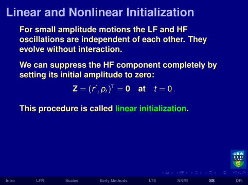
Linear and Nonlinear InitializationFor small amplitude motions the LF and HFoscillations are independent of each other. Theyevolve without interaction.
We can suppress the HF component completely bysetting its initial amplitude to zero:
Z = (r ′,pr )T = 0 at t = 0 .
This procedure is called linear initialization.
When the amplitude is large, nonlinear terms are nolonger negligible. The LF and HF motions interact.
It is clear from the equations that linear initializationwill not ensure permanent absence of HF motions . . .. . . the nonlinear LF terms generate radial momentum.
Intro LFR Scales Early Methods LTE NNMI SS DFI
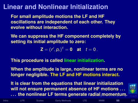
Linear and Nonlinear InitializationFor small amplitude motions the LF and HFoscillations are independent of each other. Theyevolve without interaction.
We can suppress the HF component completely bysetting its initial amplitude to zero:
Z = (r ′,pr )T = 0 at t = 0 .
This procedure is called linear initialization.
When the amplitude is large, nonlinear terms are nolonger negligible. The LF and HF motions interact.
It is clear from the equations that linear initializationwill not ensure permanent absence of HF motions . . .. . . the nonlinear LF terms generate radial momentum.
Intro LFR Scales Early Methods LTE NNMI SS DFI
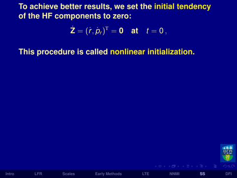
To achieve better results, we set the initial tendencyof the HF components to zero:
Z = (r , pr )T = 0 at t = 0 ,
This procedure is called nonlinear initialization.
For the spring, we can deduce explicit expressionsfor the initial conditions:
r(0) = rB ≡`(1− ε2(1− cos θ))
1− (θ/ωE)2, pr (0) = 0 .
Thus, given initial conditions X = (θ, pθ, r ,pr )T, wereplace Z = (r ,pr )T by ZB = (rB,0)T.
The rotational component Y = (θ, pθ)T is unchanged.
Does it work? An example shows that it does!
Intro LFR Scales Early Methods LTE NNMI SS DFI
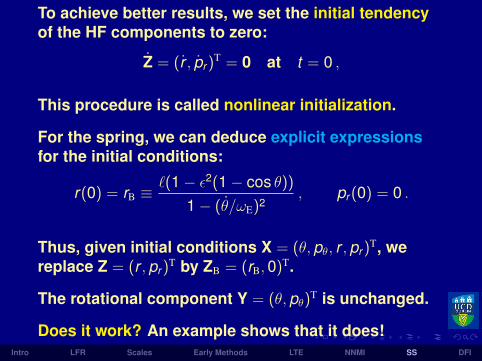
To achieve better results, we set the initial tendencyof the HF components to zero:
Z = (r , pr )T = 0 at t = 0 ,
This procedure is called nonlinear initialization.
For the spring, we can deduce explicit expressionsfor the initial conditions:
r(0) = rB ≡`(1− ε2(1− cos θ))
1− (θ/ωE)2, pr (0) = 0 .
Thus, given initial conditions X = (θ, pθ, r ,pr )T, wereplace Z = (r ,pr )T by ZB = (rB,0)T.
The rotational component Y = (θ, pθ)T is unchanged.
Does it work? An example shows that it does!Intro LFR Scales Early Methods LTE NNMI SS DFI

Solution of swinging spring equations for linear (LNMI) andnonlinear (NNMI) initialization.
Intro LFR Scales Early Methods LTE NNMI SS DFI
A Numerical ExampleIn the accompanying figure, we show the results oftwo integrations of the spring equations.
The parameter values are
m = 1 , g = π2 , k = 100π2 and ` = 1 (SI units)
Thus, ε = 0.1 and the periods of the swinging andspringing motions are respectively
τR = 2 s and τE = 0.2 s .
The initial conditions are vanishing velocity(r = θ = 0), with θ(0) = 1 and r(0) ∈
1,0.99540
.
The equations are integrated over a period of 6 s.
Intro LFR Scales Early Methods LTE NNMI SS DFI

A Numerical ExampleIn the accompanying figure, we show the results oftwo integrations of the spring equations.
The parameter values are
m = 1 , g = π2 , k = 100π2 and ` = 1 (SI units)
Thus, ε = 0.1 and the periods of the swinging andspringing motions are respectively
τR = 2 s and τE = 0.2 s .
The initial conditions are vanishing velocity(r = θ = 0), with θ(0) = 1 and r(0) ∈
1,0.99540
.
The equations are integrated over a period of 6 s.Intro LFR Scales Early Methods LTE NNMI SS DFI

Solution of swinging spring equations for linear (LNMI) andnonlinear (NNMI) initialization.
Intro LFR Scales Early Methods LTE NNMI SS DFI

The upper panels show the evolution and spectrum ofthe slow variable θ. The lower panels are for the fastvariable r .
Dotted curves are for linear initialization and solidcurves for nonlinear initialization.
For slow variable, the curves are indistinguishable.
The spectrum has a clear peak at a frequency of 0.5cycles per second (Hz).
For the fast variable, the linearly initialized evolutionhas HF noise (dotted curve, lower left panel).
This is confirmed in the spectrum: there is a sharppeak at 5 Hz.
When nonlinearly initialized, this peak is removed:only the peak at 1 Hz remains (balanced fast motion).
Intro LFR Scales Early Methods LTE NNMI SS DFI

The balanced fast motion can be understoodphysically . . .
. . . The centrifugal effect stretches the spring twicefor each pendular swing: the result is a component ofr with a period of one second.
The radial variation does not disappear for balancedmotion, but it is of low frequency.
The balanced fast motion is said to be ‘slaved’ (or,better, enslaved) to the slow motion.
Intro LFR Scales Early Methods LTE NNMI SS DFI

Solution of swinging spring equations for linear (LNMI) andnonlinear (NNMI) initialization.
Intro LFR Scales Early Methods LTE NNMI SS DFI

Outline
Introduction to Initialization
Richardson’s Forecast
Scale Analysis of the SWE [Skip]
Early Initialization Methods
Laplace Tidal Equations [Skip]
Normal Mode Initialization
The Swinging Spring [Skip]
Digital Filter Initialization
Intro LFR Scales Early Methods LTE NNMI SS DFI
The Notion of Filtering
The concept of filtering has a rôle in many fields,“from topology to theology, seismology to sociology.”
The process of filtering involves the selection ofthose components of an assemblage having someparticular property, and the removal or elimination ofthose that lack it.
A filter is any device or contrivance designed to carryout such a selection.
Intro LFR Scales Early Methods LTE NNMI SS DFI

System Diagram
The input has desired and undesired components.The output contains only the desired components.
We are primarily concerned with filters as used insignal processing.
The selection principle for these is generally basedon the frequency of the signal components.
Intro LFR Scales Early Methods LTE NNMI SS DFI

In many cases the input consists of a low-frequency(LF) signal and high-frequency (HF) noise.
The information in the signal can be isolated by usinga low-pass filter.
? ? ?
Other ideal filters can be discussed:I High-pass filtersI Band-pass filtersI Notch filters
The Low-Pass Filter is the one for initialization.
Intro LFR Scales Early Methods LTE NNMI SS DFI
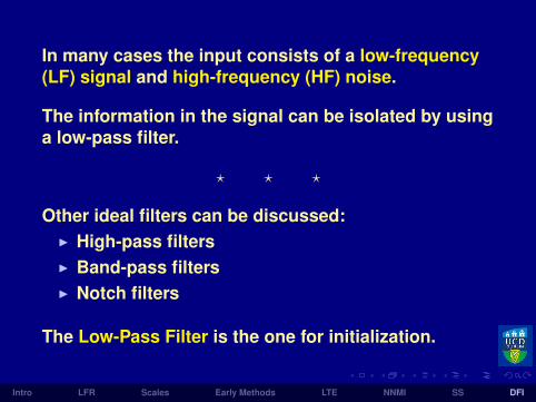
In many cases the input consists of a low-frequency(LF) signal and high-frequency (HF) noise.
The information in the signal can be isolated by usinga low-pass filter.
? ? ?
Other ideal filters can be discussed:I High-pass filtersI Band-pass filtersI Notch filters
The Low-Pass Filter is the one for initialization.
Intro LFR Scales Early Methods LTE NNMI SS DFI

Frequency response of ideal low-pass filter.
Intro LFR Scales Early Methods LTE NNMI SS DFI

Nonrecursive Filters
Given a discrete function of time,
xn
, anonrecursive digital filter is defined by
yn =N∑
k=−N
akxn−k .
The output yn depends on both past and future valuesof the input xn.
It does not depend on previous output values.
Intro LFR Scales Early Methods LTE NNMI SS DFI

Nonrecursive Filters
Given a discrete function of time,
xn
, anonrecursive digital filter is defined by
yn =N∑
k=−N
akxn−k .
The output yn depends on both past and future valuesof the input xn.
It does not depend on previous output values.
Intro LFR Scales Early Methods LTE NNMI SS DFI

Recursive Filters
A recursive digital filter is defined by
yn =N∑
k=K
akxn−k +L∑
k=1
bkyn−k
where L and N are positive integers. Usually, K = 0.
The output yn at time n∆t depends on past andpresent values of the input and also on previousoutput values.
Intro LFR Scales Early Methods LTE NNMI SS DFI
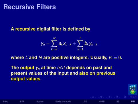
Recursive Filters
A recursive digital filter is defined by
yn =N∑
k=K
akxn−k +L∑
k=1
bkyn−k
where L and N are positive integers. Usually, K = 0.
The output yn at time n∆t depends on past andpresent values of the input and also on previousoutput values.
Intro LFR Scales Early Methods LTE NNMI SS DFI

Recursive filters are more powerful than non-recursive ones, but the feedback of the output cancause numerical instability.
The response of a nonrecursive filter to an impulseδ(n) is zero for |n| > N, giving rise to the alternativename finite impulse response or FIR filter.
The response of a recursive filter may persist: it iscalled an infinite impulse response (IIR) filter.
? ? ?
Intro LFR Scales Early Methods LTE NNMI SS DFI
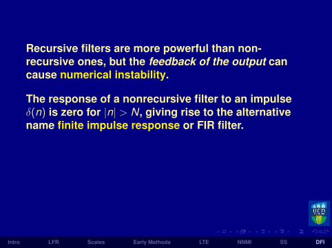
Recursive filters are more powerful than non-recursive ones, but the feedback of the output cancause numerical instability.
The response of a nonrecursive filter to an impulseδ(n) is zero for |n| > N, giving rise to the alternativename finite impulse response or FIR filter.
The response of a recursive filter may persist: it iscalled an infinite impulse response (IIR) filter.
? ? ?
Intro LFR Scales Early Methods LTE NNMI SS DFI

To find the frequency response of a recursive filter, let
xn = exp(inθ)
and assume an output of the form
yn = H(θ) exp(inθ)
Substitute yn = H(θ) exp(inθ) into the defining formula
yn =N∑
k=K
akxn−k +L∑
k=1
bkyn−k
The transfer function H(θ) is
H(θ) =
N∑k=K
ake−ikθ
1−L∑
k=1bke−ikθ
.
Intro LFR Scales Early Methods LTE NNMI SS DFI
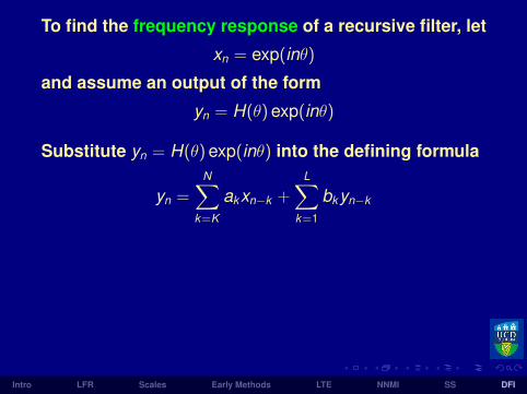
To find the frequency response of a recursive filter, let
xn = exp(inθ)
and assume an output of the form
yn = H(θ) exp(inθ)
Substitute yn = H(θ) exp(inθ) into the defining formula
yn =N∑
k=K
akxn−k +L∑
k=1
bkyn−k
The transfer function H(θ) is
H(θ) =
N∑k=K
ake−ikθ
1−L∑
k=1bke−ikθ
.
Intro LFR Scales Early Methods LTE NNMI SS DFI
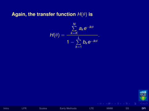
Again, the transfer function H(θ) is
H(θ) =
N∑k=K
ake−ikθ
1−L∑
k=1bke−ikθ
.
For FIR’s, the denominator reduces to unity:
H(θ) =N∑
k=−N
ake−ikθ
Intro LFR Scales Early Methods LTE NNMI SS DFI

Again, the transfer function H(θ) is
H(θ) =
N∑k=K
ake−ikθ
1−L∑
k=1bke−ikθ
.
For FIR’s, the denominator reduces to unity:
H(θ) =N∑
k=−N
ake−ikθ
Intro LFR Scales Early Methods LTE NNMI SS DFI
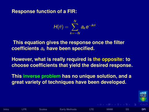
Response function of a FIR:
H(θ) =N∑
k=−N
ake−ikθ
This equation gives the response once the filtercoefficients ak have been specified.
However, what is really required is the opposite: tochoose coefficients that yield the desired response.
This inverse problem has no unique solution, and agreat variety of techniques have been developed.
The entire area of filter design is concerned withfinding filters having desired properties.
Intro LFR Scales Early Methods LTE NNMI SS DFI

Design of Nonrecursive Filters [skip]Consider a function of time, f (t), with low and highfrequency components.
To filter out the high frequencies:1. Calculate the Fourier transform F (ω) of f (t);2. Set the coefficients of the high frequencies to
zero;3. Calculate the inverse transform.
Step [2] may be performed by multiplying F (ω) by anappropriate weighting function Hc(ω).
Typically, Hc(ω) is a step function with cutoff ωc:
Hc(ω) =
1, |ω| ≤ |ωc|0, |ω| > |ωc|
Intro LFR Scales Early Methods LTE NNMI SS DFI
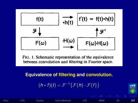
Equivalence of filtering and convolution.
(h ∗ f )(t) = F−1Fh · FfIntro LFR Scales Early Methods LTE NNMI SS DFI

These three steps are equivalent to a convolution off (t) with the inverse Fourier transform of Hc(ω):
h(t) = sin(ωct)/πt .
This follows from the convolution theorem
F
(h ∗ f )(t)
= Fh · Ff = Hc(ω) · F (ω)
Thus, to filter f (t) one calculates
f ?(t) = (h ∗ f )(t) =
∫ +∞
−∞h(τ)f (t − τ)dτ.
For simple functions f (t), this integral may beevaluated analytically. In general, someapproximation must be used.
Intro LFR Scales Early Methods LTE NNMI SS DFI
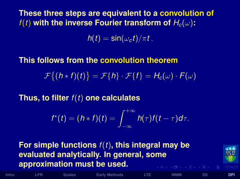

Suppose now that f is known only at discretemoments tn = n∆t , so that the sequence· · · , f−2, f−1, f0, f1, f2, · · ·
is given.
For example, fn could be the value of some modelvariable at a particular grid point at time tn.
The shortest period component which can berepresented with a time step ∆t is τNy = 2∆t ,corresponding to a maximum frequency, the so-calledNyquist frequency, ωNy = π/∆t .
Intro LFR Scales Early Methods LTE NNMI SS DFI
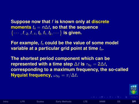
Suppose now that f is known only at discretemoments tn = n∆t , so that the sequence· · · , f−2, f−1, f0, f1, f2, · · ·
is given.
For example, fn could be the value of some modelvariable at a particular grid point at time tn.
The shortest period component which can berepresented with a time step ∆t is τNy = 2∆t ,corresponding to a maximum frequency, the so-calledNyquist frequency, ωNy = π/∆t .
Intro LFR Scales Early Methods LTE NNMI SS DFI
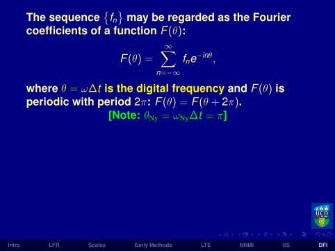
The sequence
fn
may be regarded as the Fouriercoefficients of a function F (θ):
F (θ) =∞∑
n=−∞
fne−inθ,
where θ = ω∆t is the digital frequency and F (θ) isperiodic with period 2π: F (θ) = F (θ + 2π).
[Note: θNy = ωNy∆t = π]
High frequency components of the sequence may beeliminated by multiplying F (θ) by a function Hd (θ):
Hd (θ) =
1, |θ| ≤ |θc|;0, |θ| > |θc|,
The cutoff frequency θc = ωc∆t is assumed to fall inthe Nyquist range (−π, π) and Hd (θ) has period 2π.
Intro LFR Scales Early Methods LTE NNMI SS DFI

The function Hd (θ) may be expanded:
Hd (θ) =∞∑
n=−∞hne−inθ ; hn =
12π
∫ π
−πHd (θ)einθdθ.
The values of the coefficients hn follow immediately:
hn =sin nθc
nπ.
Exercise: Prove this.
? ? ?
Let
f ?n
denote the low frequency part of
fn
, with allcomponents having frequency greater than θc removed.
Clearly,
Hd (θ) · F (θ) =∞∑
n=−∞f ?n e−inθ.
Intro LFR Scales Early Methods LTE NNMI SS DFI
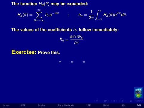
The function Hd (θ) may be expanded:
Hd (θ) =∞∑
n=−∞hne−inθ ; hn =
12π
∫ π
−πHd (θ)einθdθ.
The values of the coefficients hn follow immediately:
hn =sin nθc
nπ.
Exercise: Prove this.
? ? ?
Let
f ?n
denote the low frequency part of
fn
, with allcomponents having frequency greater than θc removed.
Clearly,
Hd (θ) · F (θ) =∞∑
n=−∞f ?n e−inθ.
Intro LFR Scales Early Methods LTE NNMI SS DFI
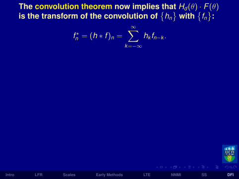
The convolution theorem now implies that Hd (θ) · F (θ)is the transform of the convolution of
hn
with
fn
:
f ?n = (h ∗ f )n =∞∑
k=−∞
hk fn−k .
This enables the filtering to be performed in the timedomain, i.e., directly on the sequence
fn
.
? ? ?
In practice the summation must be truncated: Anapproximation to the LF part of
fn
is given by
f ?n =N∑
k=−N
hk fn−k .
We see that the finite approximation to the discreteconvolution is identical to a nonrecursive digital filter.
Intro LFR Scales Early Methods LTE NNMI SS DFI
Gibbs Oscillations & Window Functions
Truncation of a Fourier series gives rise to Gibbsoscillations.
These may be greatly reduced by means of anappropriately defined “window” function.
The response of the filter is improved if hn ismultiplied by the Lanczos window:
wn =sin(nπ/(N + 1)
)nπ/(N + 1)
.
The truncated Fourier analysis of a square wave isshown in the following figures.
Intro LFR Scales Early Methods LTE NNMI SS DFI

Original Square wave function.
Intro LFR Scales Early Methods LTE NNMI SS DFI

Truncation: N = 11 (Nmax = 50)
Intro LFR Scales Early Methods LTE NNMI SS DFI

Truncation: N = 21 (Nmax = 50)
Intro LFR Scales Early Methods LTE NNMI SS DFI

Truncation: N = 31 (Nmax = 50)
Intro LFR Scales Early Methods LTE NNMI SS DFI
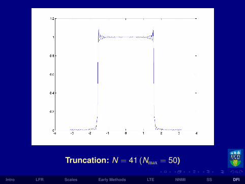
Truncation: N = 41 (Nmax = 50)
Intro LFR Scales Early Methods LTE NNMI SS DFI

Original Square wave function.
Intro LFR Scales Early Methods LTE NNMI SS DFI

Application of FIR to HiRLAM
An initialization scheme using a nonrecursive digitalfilter was developed by Lynch and Huang (1992).
The value chosen for the cutoff frequencycorresponded to a period τc = 6 hours.
With the time step ∆t = 6 minutes, this correspondsto a (digital) cutoff frequency θc = π/30.
The coefficients were derived by Fourier expansion,truncated at N = 30, with a Lanczos window:
hn =
[sin(nπ/(N + 1)
)nπ/(N + 1)
](sin(nθc)
nπ
).
Intro LFR Scales Early Methods LTE NNMI SS DFI

Application of FIR to HiRLAM
The use of the window de-creases the Gibbs oscillations inthe stop-band |θ| > |θc |.
However, it also has the effect ofwidening the pass-band beyondthe nominal cutoff.
Intro LFR Scales Early Methods LTE NNMI SS DFI

Application of FIR to HiRLAM
The central lobe of the coefficient function spans aperiod of six hours, from t = −3 h to t = +3 h:TSpan = 6 hours.
The filter summation was calculated over this range,with the coefficients normalized to have unit sumover the span.
Thus, the application of the technique involvedcomputation equivalent to sixty time steps, or a sixhour integration.
? ? ?
Intro LFR Scales Early Methods LTE NNMI SS DFI
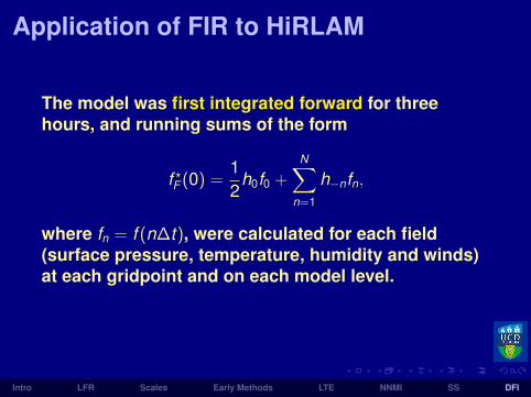
Application of FIR to HiRLAM
The model was first integrated forward for threehours, and running sums of the form
f ?F (0) =12
h0f0 +N∑
n=1
h−nfn,
where fn = f (n∆t), were calculated for each field(surface pressure, temperature, humidity and winds)at each gridpoint and on each model level.
These were stored at the end of the 3 hr forecast.
Intro LFR Scales Early Methods LTE NNMI SS DFI

The original fields were then used to make a threehour ‘hindcast’, during which running sums
f ?B(0) =12
h0f0 +−N∑
n=−1
h−nfn
were computed for each field, and stored as before.
The two sums were then combined to give
f ?(0) = f ?F (0) + f ?B(0) =N∑
n=−N
h−nfn .
These fields correspond to the application of thedigital filter to the original data.
They are the filtered data.
Intro LFR Scales Early Methods LTE NNMI SS DFI

The original fields were then used to make a threehour ‘hindcast’, during which running sums
f ?B(0) =12
h0f0 +−N∑
n=−1
h−nfn
were computed for each field, and stored as before.
The two sums were then combined to give
f ?(0) = f ?F (0) + f ?B(0) =N∑
n=−N
h−nfn .
These fields correspond to the application of thedigital filter to the original data.
They are the filtered data.Intro LFR Scales Early Methods LTE NNMI SS DFI

Phase ErrorsIn the foregoing, only the amplitudes of the transferfunctions have been discussed.
Since these functions are complex, there is also aphase change induced by the filters.
We will not consider this question here. However, it isessential that the phase characteristics of a filter bestudied before it is considered for use.
Ideally, the phase-error should be as small aspossible for the low frequency components which aremeteorologically important.
Recall that phase-errors are amongst the mostprevalent and pernicious problems in forecasting.
Intro LFR Scales Early Methods LTE NNMI SS DFI

The Dolph-Chebyshev Filter
We now consider a particularly simple filter, havingexplicit expressions for its impulse responsecoefficients.
We give here the definition and principal properties ofthe Dolph-Chebyshev filter.
For further information, see Lynch, 1997(http://maths.ucd.ie/∼plynch)
Intro LFR Scales Early Methods LTE NNMI SS DFI
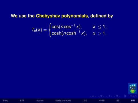
We use the Chebyshev polynomials, defined by
Tn(x) =
cos(n cos−1 x), |x | ≤ 1;
cosh(n cosh−1 x), |x | > 1.
Clearly, T0(x) = 1 and T1(x) = x .
A recurrence relation follows from the definition:
Tn(x) = 2xTn−1(x)− Tn−2(x), n ≥ 2.
In the interval |x | ≤ 1, Tn(x) varies between +1 and −1.
Intro LFR Scales Early Methods LTE NNMI SS DFI

Now consider the function defined in the frequencydomain:
H(θ) =T2M (x0 cos (θ/2))
T2M(x0),
where x0 > 1.
Let θs be such that x0 cos(θs/2) = 1:I As θ varies from 0 to θs, H(θ) falls from 1 to
r = 1/T2M(x0).I For θs ≤ θ ≤ π, H(θ) oscillates in the range ±r .
The form of H(θ) is that of a low-pass filter with acut-off at θ = θs.
H(θ) can be written as a finite expansion:
Intro LFR Scales Early Methods LTE NNMI SS DFI
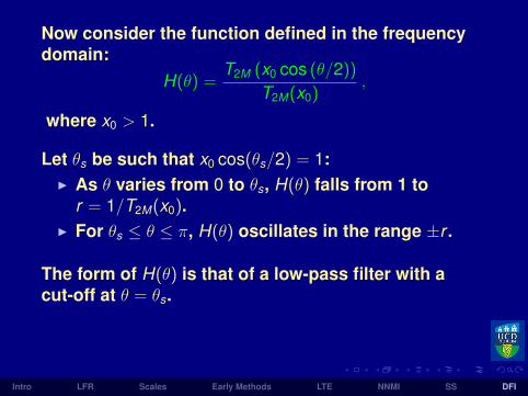
Now consider the function defined in the frequencydomain:
H(θ) =T2M (x0 cos (θ/2))
T2M(x0),
where x0 > 1.
Let θs be such that x0 cos(θs/2) = 1:I As θ varies from 0 to θs, H(θ) falls from 1 to
r = 1/T2M(x0).I For θs ≤ θ ≤ π, H(θ) oscillates in the range ±r .
The form of H(θ) is that of a low-pass filter with acut-off at θ = θs.
H(θ) can be written as a finite expansion:
Intro LFR Scales Early Methods LTE NNMI SS DFI
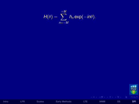
H(θ) =+M∑
n=−M
hn exp(−inθ).
The coefficients hn may be evaluated from theinverse Fourier transform
hn =1N
[1 + 2r
M∑m=1
T2M
(x0 cos
θm
2
)cos mθn
],
where |n| ≤ M, N = 2M + 1 and θm = 2πm/N.
Since H(θ) is real and even, hn are also real andh−n = hn.
The weights hn : −M ≤ n ≤ +M define theDolph-Chebyshev or, for short, Dolph filter.
Intro LFR Scales Early Methods LTE NNMI SS DFI
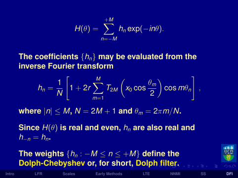
H(θ) =+M∑
n=−M
hn exp(−inθ).
The coefficients hn may be evaluated from theinverse Fourier transform
hn =1N
[1 + 2r
M∑m=1
T2M
(x0 cos
θm
2
)cos mθn
],
where |n| ≤ M, N = 2M + 1 and θm = 2πm/N.
Since H(θ) is real and even, hn are also real andh−n = hn.
The weights hn : −M ≤ n ≤ +M define theDolph-Chebyshev or, for short, Dolph filter.
Intro LFR Scales Early Methods LTE NNMI SS DFI

In the HiRLAM model, the filter order N = 2M + 1 isdetermined by the time step ∆t and forecast span TS.
The desired frequency cut-off is specified bychoosing a value for the cut-off period, τs.
Then θs = 2π∆t/τs and the parameters x0 and r are
1x0
= cosθs
2,
1r
= cosh(
2M cosh−1 x0
).
The ripple ratio r is a measure of the maximumamplitude in the stop-band [θs, π]:
r =
[side-lobe amplitudemain-lobe amplitude
]
The Dolph filter has minimum ripple-ratio for a givenmain-lobe width and filter order.
Intro LFR Scales Early Methods LTE NNMI SS DFI
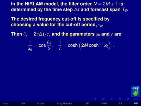
In the HiRLAM model, the filter order N = 2M + 1 isdetermined by the time step ∆t and forecast span TS.
The desired frequency cut-off is specified bychoosing a value for the cut-off period, τs.
Then θs = 2π∆t/τs and the parameters x0 and r are
1x0
= cosθs
2,
1r
= cosh(
2M cosh−1 x0
).
The ripple ratio r is a measure of the maximumamplitude in the stop-band [θs, π]:
r =
[side-lobe amplitudemain-lobe amplitude
]
The Dolph filter has minimum ripple-ratio for a givenmain-lobe width and filter order.
Intro LFR Scales Early Methods LTE NNMI SS DFI

Example of Dolph FilterSuppose components with period less than threehours are to be eliminated (τs = 3 h) and the time stepis ∆t = 1
8 h.
The parameters chosen for the DFI are:I Span TS = 2 hI Cut-off period τs = 3 hI Time step ∆t = 450 s = 1
8 h
So, M = 8, N = 17 and θs = 2π∆t/τs ≈ 0.26.
The DFI procedure employed in the HIRLAM modelinvolves a double application of the filter.
We examine the frequency response H(θ) and itssquare, H(θ)2 (a second pass squares the frequencyresponse).
Intro LFR Scales Early Methods LTE NNMI SS DFI
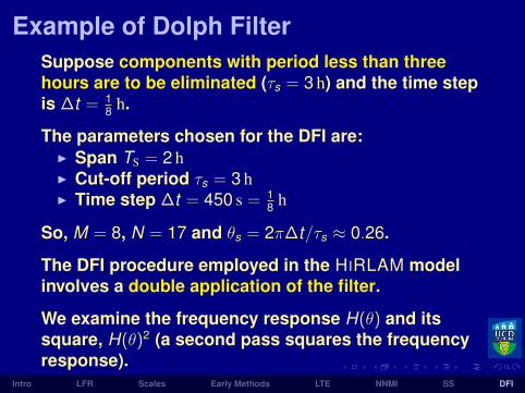
Example of Dolph FilterSuppose components with period less than threehours are to be eliminated (τs = 3 h) and the time stepis ∆t = 1
8 h.
The parameters chosen for the DFI are:I Span TS = 2 hI Cut-off period τs = 3 hI Time step ∆t = 450 s = 1
8 h
So, M = 8, N = 17 and θs = 2π∆t/τs ≈ 0.26.
The DFI procedure employed in the HIRLAM modelinvolves a double application of the filter.
We examine the frequency response H(θ) and itssquare, H(θ)2 (a second pass squares the frequencyresponse).
Intro LFR Scales Early Methods LTE NNMI SS DFI

Frequency response for Dolph filter with span TS = 2h, order N = 2M + 1 = 17and cut-off τs = 3h. Results for single and double application are shown.
Logarithmic response (dB) as a function of frequency.
Intro LFR Scales Early Methods LTE NNMI SS DFI

Frequency response for Dolph filter with span TS = 2h, order N = 2M + 1 = 17and cut-off τs = 3h. Results for single and double application are shown.
Amplitude response as a function of period.
Intro LFR Scales Early Methods LTE NNMI SS DFI
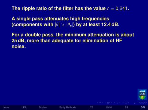
The ripple ratio of the filter has the value r = 0.241.
A single pass attenuates high frequencies(components with |θ| > |θs|) by at least 12.4 dB.
For a double pass, the minimum attenuation is about25 dB, more than adequate for elimination of HFnoise.
The amplitudes of components with periods less thantwo hours are reduced to less than 5%.
Components with periods greater than one day areleft substantially unchanged.
It can be proved (Lynch, 1997) that the Dolph windowis an optimal filter whose pass-band edge, θp, is thesolution of the equation H(θ) = 1− r .
Intro LFR Scales Early Methods LTE NNMI SS DFI
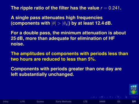
The ripple ratio of the filter has the value r = 0.241.
A single pass attenuates high frequencies(components with |θ| > |θs|) by at least 12.4 dB.
For a double pass, the minimum attenuation is about25 dB, more than adequate for elimination of HFnoise.
The amplitudes of components with periods less thantwo hours are reduced to less than 5%.
Components with periods greater than one day areleft substantially unchanged.
It can be proved (Lynch, 1997) that the Dolph windowis an optimal filter whose pass-band edge, θp, is thesolution of the equation H(θ) = 1− r .
Intro LFR Scales Early Methods LTE NNMI SS DFI
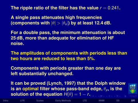
The ripple ratio of the filter has the value r = 0.241.
A single pass attenuates high frequencies(components with |θ| > |θs|) by at least 12.4 dB.
For a double pass, the minimum attenuation is about25 dB, more than adequate for elimination of HFnoise.
The amplitudes of components with periods less thantwo hours are reduced to less than 5%.
Components with periods greater than one day areleft substantially unchanged.
It can be proved (Lynch, 1997) that the Dolph windowis an optimal filter whose pass-band edge, θp, is thesolution of the equation H(θ) = 1− r .
Intro LFR Scales Early Methods LTE NNMI SS DFI
Implementation in HIRLAM
The digital filter initialization is performed by applyingthe filter to time series of model variables.
The filter is applied in two stages:
In the first stage, a backward integration from t = 0 tot = −TS is performed, with all irreversible physicsswitched off.
The filter output is calculated by summing:
x =n=−N∑n=0
hN−nxn .
The output x is valid at time t = −12TS.
Intro LFR Scales Early Methods LTE NNMI SS DFI
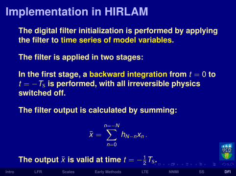

In the second stage, a forward integration is madefrom t = −1
2TS to t = +12TS, starting from the output x .
Again, the filter is applied by accumulating sumsformally identical to those of the first stage.
The output of the second stage is valid at the centreof the interval [−1
2TS,+12TS], i.e., at t = 0.
The output of the second pass is the initialized data.
Intro LFR Scales Early Methods LTE NNMI SS DFI

Intro LFR Scales Early Methods LTE NNMI SS DFI

DFI: Sample Results
The basic measure of noise is the mean absolutevalue of the surface pressure tendency
N1 =
(1
NGRID
) NGRID∑n=1
∣∣∣∣∂ps
∂t
∣∣∣∣ .
For well-balanced fields this quantity has a value ofabout 1 hPa per 3 hours.
For uninitialized fields, it can be up to an order ofmagnitude larger.
In the following figure, we plot the value of N1 forthree forecasts.
Intro LFR Scales Early Methods LTE NNMI SS DFI
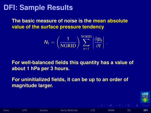
DFI: Sample Results
The basic measure of noise is the mean absolutevalue of the surface pressure tendency
N1 =
(1
NGRID
) NGRID∑n=1
∣∣∣∣∂ps
∂t
∣∣∣∣ .For well-balanced fields this quantity has a value ofabout 1 hPa per 3 hours.
For uninitialized fields, it can be up to an order ofmagnitude larger.
In the following figure, we plot the value of N1 forthree forecasts.
Intro LFR Scales Early Methods LTE NNMI SS DFI

Mean absolute surface pressure tendency for threeforecasts. No initialization (NIL); Normal mode initialization
(NMI); Digital filter initialization (DFI). (Units hPa/3 h)
Intro LFR Scales Early Methods LTE NNMI SS DFI

The measure N1 indicates the noise in the verticallyintegrated divergence field.
However, even when this is small, there may besignificant activity in the internal gravity wave modes.
To see this, we look at the vertical velocity field at500 hPa for the NIL and DFI analyses.
? ? ?
The uninitialized vertical velocity field is physicallyquite unrealistic.
The DFI vertical velocity is much smoother, and muchmore realistic.
Intro LFR Scales Early Methods LTE NNMI SS DFI

Vertical velocity at 500 hPa for uninitialized analysis (NIL).
Intro LFR Scales Early Methods LTE NNMI SS DFI

Vertical velocity at 500 hPa after digital filtering (DFI).
Intro LFR Scales Early Methods LTE NNMI SS DFI
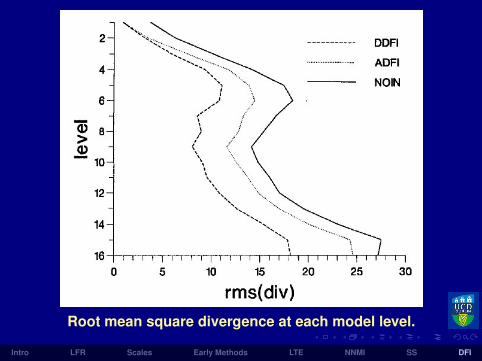
Root mean square divergence at each model level.
Intro LFR Scales Early Methods LTE NNMI SS DFI
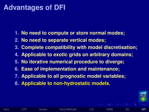
Advantages of DFI
1. No need to compute or store normal modes;2. No need to separate vertical modes;3. Complete compatibility with model discretisation;4. Applicable to exotic grids on arbitrary domains;5. No iterative numerical procedure to diverge;6. Ease of implementation and maintenance;7. Applicable to all prognostic model variables;8. Applicable to non-hydrostatic models.
Intro LFR Scales Early Methods LTE NNMI SS DFI

Thank you
Intro LFR Scales Early Methods LTE NNMI SS DFI