balanced aspect ratio trees:: combining the …goodrich/pubs/bar-soda.pdfbalanced aspect ratio...

300

Balanced Aspect Ratio Trees:: Combining the Advantages of k-d Trees (and Octrees

CHRISTIAN A. DUNCAN* MICHAEL T. GOODRICH+ Center for Geometric Computing Center for Geometric Computing

The Johns Hopkins University The Johns Hopkins University

[email protected] [email protected]

STEPHEN KOBOUROV~

Center for Geometric Computing

The Johns Hopkins University

[email protected]

Abstract

Given a set S of n points in lRd, we show, for fixed d, how to construct in O(n log n) time a data structure we call the Balanced Aspect Ratio (BAR) tree. A BAR tree is a binary space partition tree on S that has O(logn) depth and in which every region is convex and “fat” (that is, has a bounded aspect ratio). While previous hierarchical data structures, such as k-d trees, quadtrees, octrees, fair-split trees, and balanced box decompositions can guarantee some of these properties, we know of no previous data structure that combines alI of these properties simultaneously. The BAR tree data structure has numerous applications ranging from solving several geometric searching problems in fixed dimensional space to aiding in the visualization of graphs and three-dimensional worlds.

1 Introduction

Geometric searching of multi-dimensional spaces is a fundamental operation in many fields, including as- tronomy, geographic information systems (GIS), computer graphics, information retrieval, pattern recogni- tion, natural language processing, and statistics. Typ- ical searches include nearest-neighbor searches, farthest- neighbor searches, and range queries (which are intersection queries for geometric shapes). In this paper we study efficient data structures for performing such queries in moderate-dimensional spaces, that is, in spaces where the dimensionality, d, of the space can be viewed as a constant compared to the number, n, of multi- dimensional points in that space’.

This research partially supported by AR0 under grant DAAH04-96-1-0013.

fThis research partially supported by NSF under Grant CCR- 9625289, and AR0 under grant DAAH0496-l-0013.

SThis research partially supported by AR0 under grant DAAHO496-1-0013.

1 We will view d as a constant relative to n throughout this paper.

1.1 Previous Work. Data structures for performing multi-dimensional geometric searching in moderate- dimensional spaces is a well-studied problem in compu- tational geometry and spatial databases. Many previous data structures for performing geometric searching for a multi-dimensional point set S are instances of a general class of structures known as binary space partition (BSP) trees [16] (see also 1271). Each node in a BSP tree T represents both a convex region in space and aI of the points of S lying inside this region. Each leaf node in T represents a region with a constan! number of points of S inside it. Every other node in T has an associated hyperplane cut partitioning the region into two subregions, each corresponding to a child node. The root of T is associated with a bounding hyperbox containing S. One of the main advantages of BSP trees is that they allow for simple multi-dimensional searching, with a typical comparison for a node v in T simply involving a sidedness test against the hyperplane cut associated with 21. BSP trees are used often to solve problems in computer graphics [ll, 23, 24, 281, such as global illu- mination, shadow generation, ray casting, and visibility. They are also used in information retrieval for finding nearest neighbors, farthest neighbors, and performing range queries.

The performance bounds of a BSP tree T for answering such queries for a point set S are directly related to the depth of T and the “fatness” [2, 14, 201 (that is, the boundedness of the aspect ratios) of the regions associated with T’s vertices. One well-known class of BSP trees, known as k-d trees [6, 7, 17, 221, uses axis-parallel cutting hyperplanes that are placed so as to divide the set of points associated with a node more-or-less in half. Such trees have excellent depth properties, in that their depth is always O(log n). Unfortunately, since the objects in S are points, which are not themselves fat (as with the sets of objects studied in [l, 12, 21]), the regions associated with vertices in a k-d tree can have arbitrarily large aspect

301

ratios. This unbounded aspect ratio property of k- d trees partly accounts for why there are few simple theoretical results better than the O(nl-lld) average running time, even for approximation versions.

Another well-known class of search structures, known as quadtrees [15, 25, 271 and octrees [3, 10, 18, 261, are based on the alternate approach of using axis- parallel hyperplanes to divide region volumes equally. These structures produce space partitioning trees with regions having good aspect ratios, but their depths can be quite large, which again results in poor worst-case search times.

These poor worst-case performances of k-d trees and octrees have motivated some researchers to abandon the BSP tree framework altogether in search of alternate structures with good depth and aspect-ratio bounds. ln particular, the balanced box-decomposition (BBD) tree structure of Arya et al. [S, 41, which is based on the fair-split tree of Callahan and Kosaraju [8, 91, provides a space partitioning tree that has O(logn) depth while also achieving vertex-associated regions with bounded aspect ratios. Arya et al. show that this structure can be used, for example, to perform approximate nearest- neighbor searching and range searching in O(logn + k) time, where k is the size of the output. The only draw- back with this approach is that it partitions space using non-hyperplanar cuts with “holes,” which sacrifices the convexity property for vertex-associated regions. This sacrifice makes the BBD tree inappropriate for several applications in computer graphics and graph drawing, where convexity of the partitioned regions is desirable (e.g., see [19]).

1.2 Our Results. Building on earlier work of the authors for a two-dimensional balanced space partition data structure [13], useful in the context of graph drawing, we introduce in this paper a multi-dimensional space partition tree data structure, which we call the balanced aspect ratio (BAR) tree, that is defined for any set S of n points in lRd. The BAR tree data structure is conceptually quite simple, for it follows the traditional format of the binary space partition (BSP) tree. Moreover, BAR trees simultaneously achieve the desired properties of having O(log n) depth and vertex- associated regions that are convex and “fat” (having bounded aspect ratios).

In the following sections, we give a general framework for BAR trees, some geometric searching applications that are realized by BAR trees, and finally give

the latter of which we call “corner cuts.” This method can be viewed as an extension of the traditional k-d tree, for our BAR tree is identical to the k-d tree defined on S so long as the k-d tree maintains a balanced aspect ratio; we only use corner cuts when an axis-parallel cut would produce a region that is too “skinny.”

2 The General BAR Tree Framework

In this section, we develop a general framework for constructing BAR trees. We begin by defining what we mean by bounded aspect ratio.

DEFINITION 2.1. A convex region R in IRd has aspect ratio asp(R) = OR/IR with respect to some underlying metric, where OR is the radius of the smallest circum- scribed hypersphere in Rd and IR is the radius of the largest inscribed d-hypersphere. R has balanced aspect ratio with maximum aspect ratio CY 2 1, if asp(R) 5 (Y. We say, a region R is an a-balanced region if it has maximum aspect ratio cr. A collection of regions, R, has balanced aspect ratio with balancing factor cz if each region R E R is an a-balanced region.

Typically, we use one of the standard L, metrics to define aspect ratios, as these are all within a polynomial factor of d from each other. In keeping with current custom [2, 14, 201, we use the terms fat and skinny to refer to regions which have respectively balanced and unbalanced aspect ratios. This definition states that a region R has a minimum width associated with its diameter. As in Arya et al. [S], we use this property to show worst-case bounds on some geometric approximation problems.

DEFINITION 2.2. A canonical cut set, C = {G,vi,.. . , $1, is a collection of y, not necessar- ily independent, vectors that span Rd (thus, 7 2 d). A canonical cut is any hyperplane, H, in Rd with a normal in C. A canonical retion is a convex polyhedron in lRd with every facet having a normal in C.

DEFINITION 2.3. Any two canon&~I cuts H and H’ that are normal to the same vector in C, i.e. parallel to each other, are opposing canonical cuts. For any bounded region R, define the canonical bounding cuts with respect to a direction v’i E C to be the two unique opposing C~IIO~~C~ cuts normal to v’i, and tangent to R. Intuitively, R is “sandwiched” between the two opposing cuts. -

an efficient method for constructing a BAR tree. Our method for constructing a BAR tree for a point set S

The canonical set used to define a partition tree

uses hyperplane cuts that are either parallel to a co- can vary from method to method. For example, the

ordinate axis or form 45” angles with coordinate axes, standard k-d tree algorithm uses a canonical set, of all axis-parallel directions. For notation, we often refer to

302

a canonical cut by its normal vector, Gi E C. In the k-d tree model, we would represent a cut along the y-axis by (0, LO,. . . , 0). We refer to such an opposing pair by its direction, fli E C, in positive or negative form of the normal vector. Also, let (R( represent the number of points from a given data set S contained in the region R, i.e. its size in terms of points rather than volume.

DEFINITION 2.4. An o-balanced canonical region, R, is one-c&table with reduction factor P, where l/2 5 p < 1, if there is a cut s1 E C, called a one-cut, dividing R into two subregions RI and R2 such that

1. RI and R2 are o-balanced canonical regions,

2. IRll L PIRI and lR2I I PIRI.

DEFINITION 2.5. An o-balanced canonical region, R, is k-c&table with reduction factor P, for k > 1, if there is a cut sk E C, called a k-cut, dividing R into two subregions RI and R2 such that

1. RI and R2 are o-balanced canonical regions,

2. lR2l I PIRI, 3. Either jR1 I 5 p/RI or RI is (k - I)-cuttable with

reduction factor p.

In other words, the sequence of cuts, sk,sk--17...,sl, results in k + 1 balanced canonical regions each containing no more than pn points. If p is understood, we simply say R is k-cuttable.

THEOREM 2.1. For a canonical set, C, if every possible o-balanced canonical region is k-cuttable with reduction factor fi, then a BAR tree with maximum aspect ratio Q can be constructed with depth O(k logrlp n), for any set S of n points.

Proof. Start with an initial bounding a-balanced canonical region on S. Since this region is k-cuttable, use a sequence of k cuts to divide the region into k + 1 o-balanced canonical subregions each containing fewer than ,f?n of the points. Repeat this process on each of the resulting subregions until a subregion has less than some constant number of points. The process, down any path of subregions, can be repeated for no more than O(logrlp n) times, resulting in the stated tree depth bound. H

The main challenge in creating a specific instance of a BAR tree is in defining a canonical set C such that every possible o-balanced canonical region is k-cuttable with reduction factor ,S for reasonable choices of a, P, and k. But, before we do this, let us motivate it by describing a few applications for BAR trees.

3 BAR Tree Applications

Suppose we are given a point set S of n points in Rd using any one of the Minkowski L, metrics. After constructing a BAR tree T on S, we are able to perform some useful queries. For any query point q E lRd, we are able to efficiently report both the approximate-nearest and approximate-farthest neighbors of q in S. If we are also given a radius T, we are able to efficiently return all points within a distance T from q plus possibly any points that are approximat6ely near P, which is a form of approximate range searching. We will more formally describe some of these applications shortly.

Arya et al. [4, 5] propose a technique to solve the approximate nearest-neighbor and range query problems by constructing a balanced box-decomposition tree. Similar to our BAR trees, these trees maintain an o-balanced aspect ratio but only by introducing non- convex hole cuts. Their arguments and techniques for solving these query problems, however, are easily trans- ferable to our data structure.

DEFINITION 3.1. For a set S of points in Rd, a query point q E lRd, and E > 0, a point p E S is a (1+ E)- nearest neighbor of q if d(p, q) 5 (1 + e)bCpf , q), where p* is the true nearest neighbor to q.

In other words, such a p is within a constant error factor of the true nearest neighbor. This definition can also be extended to report a sequence of s (1 + e)-nearest neighbors. Rather than adapt all theorems presented by Arya et al. in this extended abstract, we instead prove another useful query operation, applicable to both their and our methods, and establish an important packing feature for BAR trees.

DEFINITION 3.2. For a set S of points in IRd, a query point q E lRd, and E > 0, a point p E S is a (1 - E)- farthest neighbor of q if b(p, q) > dw, q) - ED, where p* is the true farthest neighbor and D is the diameter of the point set.

We are using an absolute error bound rather than the standard relative error, b(p,q) 1 (1 - e)&(p’,q), because the bound is tighter in every case. Imagine a point set that is tightly contained in the unit sphere, and a query point that is extremely, 100/e units, far from this sphere. Now, any point returned would be a (1 - e)-farthest neighbor of S using a relative error bound. In our definition, a query point is the better of the absolute and relative distances, within a constant factor of E. Since D is the diameter of the set, any query point must be at least half the diameter away from one of the points in the set, d(p*,q) 2 D/2. Letting E’ = 2e,

303

we see that must contain the real point that was farthest from g.

f&q) L 4p*,q) -ED 2 6(p’,q) - c2b03f,q) = (1- 2e)6(p’,q) = (1 - e’)6(p8,q).

Wlog, let this be ‘1~1 and insert 2~2 into the queue. Use u1 as next “extracted” node from Q and continue.

Hence, using an absolute error bound in the approximate farthest-neighbor query always gives a point whose distance is at least as far as the distance obtained using a relative error bound. In fact, one can extend this notion and our arguments to compensate for this problem in nearest-neighbor queries as well, i.e., when the query point is relatively far away from the entire data set.

We now, briefly, discuss the farthest neighbor approximation algorithm using a BAR tree. Given our query point q, we begin by finding a leaf node that is the farthest away from q. Here, a region’s maximum distance from a point is considered, implying that, in theory, the node containing the point q might still also be the node that is the farthest from q. We next enu- merate, via a priority queue, all leaf nodes in decreasing order of distance, i.e. farthest leaf nodes first. For every leaf node, we compute the distance between that node’s data point and q and maintain the current farthest visited point. When the distance between q and the current farthest node is less than J&J, q) + CD, we can terminate the search, as b(p*,q) < 6(p,q) + ED.

A priority queue can be maintained in such a way that the running time is O(logn) times the number of leaf nodes visited. The key to the algorithm’s success is that the number of leaf nodes visited can be liited by using a packing argument. Let us, therefore, describe both the priority queue technique and the packing argument needed to limit the number of leaf nodes visited.

LEMMA 3.1. Given a BAR tree T with depth O(k log,,8 n) and y canonical vectors, for any query point q, a (1 - c)-farthest neighbor to q can be found in O(kZy log,,p n) time, where 1 is the number of leaf nodes visited in our algorithm.

Proof. First we can see the correctness of our algorithm by looking at the leaf node U* containing p’. If U* has been visited, our algorithm would set p t p’ and return the correct solution upon termination. If u* has not yet been visited, implying p # p’, we see that &P*, d 5 &‘LL*> 4 5 d(u, d I G, q) + ED.

Now, let u be any node that is extracted from the queue. Since our algorithm does not do another extract operation until it reaches a leaf node which has depth O(k logrlp n), we perform O(k log,,p n) queue inserts per leaf node visited and one extract per leaf node. If we use a Fibonacci heap, although in practice this would not be necessary, insertions take O(1) amortized time and extractions take O(logn), since the queue has size O(kn). At each split, deciding which node is farther takes 0(-y) time as the node regions have O(r) complexity. Thus, if 1 is the number of leaf nodes visited, the algorithm terminates in O(kZrlogllp n) steps. n

3.2 Packing Constraint. Thus, as in the nearest- neighbor algorithm of Arya et al., if we can liiit the number of leaf nodes that we need to visit, the running time would be known. This is where a packing constraint comes in.

3.1 Searching Farthest Nodes. Let us describe, LEMMA 3.2. (Packing Lemma) Given a BAR tree

in more detail, the searching technique which uses the with maximum aspect ratio cr for a set S of data points

priority queue. To avoid confusion between points in in Rd and two size parameters r,r’ > 0, using any

space and in the data set, we call a point p, a data point Miiowski metric, L,, there are O((a&)d(r/r’)d-‘)

if p E S, and a point T, a real point if r E Rd. For leaf nodes which pierce any annulus with radii r + r’

any node u and its associated region R, let a(u,q) = and r- d(R, q) = maxIERS(r,q), i.e. the distance between q and a node u is the distance between q and the farthest real point from q in the region R.

Initially, a priority queue Q starts with the root node of T. Let p be the current farthest neighbor, initially set to q. At every stage, extract from Q the node, u, that is the farthest from q. If 4% d < 6(p, q) + ED, we return p as the (1 f e)-approximate farthest neighbor. If u is a leaf node, let p’ E S be the node’s associated data point, if any. If 6(p’, q) > 6(p, q), let p t p’. Remove u from consideration, and continue with the next node in Q. If u is not a leaf, let ur and us be u’s children. Since u = u1 U 112, one of the two nodes

Proof. Let 1 be a leaf node in the tree with associated region R that pierces the annulus, A. This means that the outer radius OR 2 r’. Since the region is CY- balanced, recall that the inner radius of R, IR 2 0~1~. We then know that the volume of R, in any metric, is greater than the volume of the L1 hypersphere, a diamond in the plane,

VR 2 (21~/&i)~ 1(20~/(oJ;i))~ 2 (2r’l@hNd,

and because the objects are convex, the intersection B = An R has volume VB 2 (2r’/(cx&))d. Now, in any metric, the volume of any annulus, A, of radius

304

r + r’, r is less than or equal to the difference between the volume of the outer and inner boxes of length +-- 2(r + r’) and 2r respectively, the L, metric. This, VA 5 (2r + 2r’)d - (2r)d = (2r)d((l + r’/r)d - 1).

Since the leaf nodes do not overlap, the number of leafs nodes, L, is larger than the ratio of the two volumes, L 5 VA/I& _< (caQd((r/r’ + l)d - (r/r’)d) =

O((ad2)d(r/r’)d-1). n

Our only other concern, then, is that some leaf nodes might not contain any points, as we never made this stipulation in our general framework, although this scenario is highly unlikely. This problem is averted by noticing that since the regions are all k-cuttable, there are at most k - 1 regions in sequence that can be empty, as after k cuts two regions must both have less than a p fraction of the points. We then defer the costs for an empty leaf node to one of the non-empty leaf nodes in its sibling’s region. As there is an actual split after every k - 1 cuts, we can ensure that no leaf node gets more than k of the deferred charges, so the running time increases by at most a factor of k.

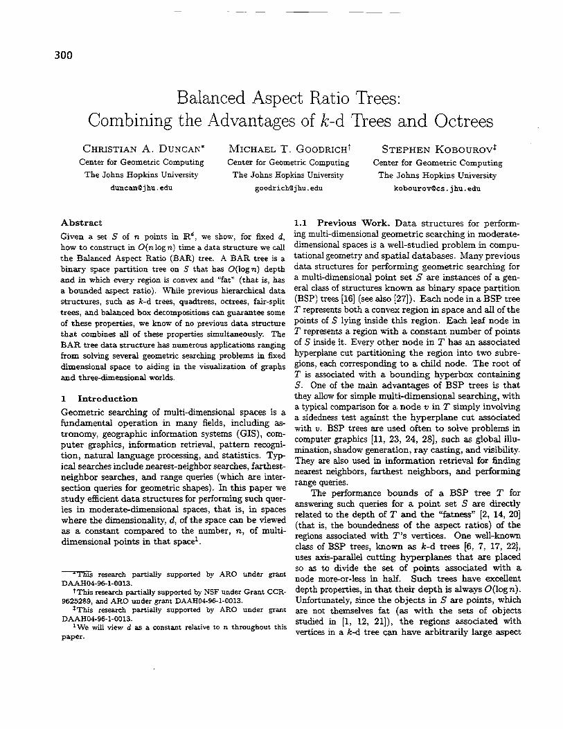
Figure 1: The notion of corner cuts. (a) A corner cut in the plane. (b) A corner cut in 3-d.

along any face forces the next cut to either be too close to the opposing face or not divide a significant portion of the points in the region, resulting in an unbalanced depth. Our solution is to introduce a simple comer cut that yields enough freedom of direction to construct a BAR tree.

DEFINITION 4.1. A corner cut in Rd is a hyperplane whose normal vector is of the form (10, 11, . . . , Id) where Ii E {1,-l}.

:’

L I

THEOREM 3.1. Suppose we are given a BAR tree T with depth O(klog,,p n), a balancing factor o, and 7 canonical vectors, on a point set S with diameter D and n data points. For any query point Q, a (1 - c)-farthest neighbor to Q can be found in O(k2-y(a&)d(l/c)d-1 logn) time.

Proof. For any leaf node visited, but the last, U, b(~, Q) > S@, 9) + ED, as this was the halting condition. Also, every leaf node visited, U, which contained a point, p’, had to have b(p’, q) 5 b(p, q) by the fact that p was the farthest point found. Thus, similar to the method of Arya et al. [5], we know that every node containing a point visited by the algorithm must completely pierce the annulus of radii a(p, q) and b(p, q) + ED, i.e. he on both sides of this annulus. Since the diameter of the point set is S, every leaf node containing a point must also he at least partly inside a ball of radius D. Any leaf node piercing the original annulus, therefore, also pierces an annulus with radii D and D(1 + E). In ap- plying the Packing Lemma (3.2), Lemma 3.1, and our compensation for empty leaf nodes, we get a running time of O(kylog,,B n * (cx&)~(D/(ED))~-~ * k), and the stated bound follows. n

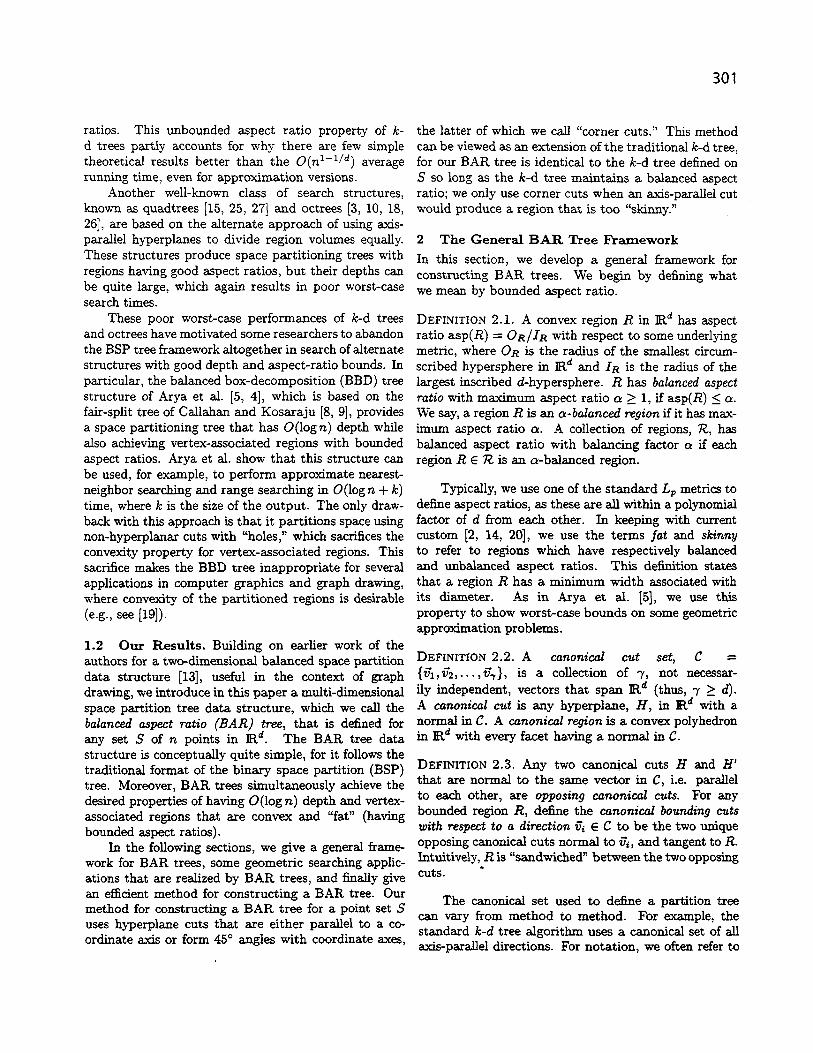
For a region R, canonical with respect to C, consider a direction vector Gi E C. Let widt&(R) be the distance between the two bounding canonical cuts of R normal to Gi. For simplicity, let us normalize the distance between two opposing planes by using the L, metric. In a region R, this means that for two bounding canonical comer cuts p and q with normal Gi whose equations are of the form p : v’iiz’ = a and q : f&Z = b, the width widt&(R) = 9 (see Figure 2-a). 4 Corner-Cut BAR Trees

We now show a specific instance of a BAR tree. Ideally, Notice, since the normal vector to a corner cut

in constructing a BAR tree we would prefer to use only forms a 45’ angIe with each axis, the regular Euclidean axis-parallel cuts, but this is not possible. If, for ex- distance between the planes is ?a. The distances ample, the vast majority of the points are concentrated between two axis-parallel cuts in the L, metrics are all at a particular corner of a hyperbox region, cutting identical, for p E (1,. . . , oo}. Thus, using any other L,

Notice that there are 2d possible corner cuts corresponding to all combinations of fl. In the plane, such a cut forms a 45” angle with both the x- and y-axes (see Figure 1). The advantage to using these corner cuts will soon become apparent. Let us therefore show how to use such cuts to define a canonical cut set that is sufficient for constructing an efficient BAR tree.

Cauouical Cut Set: Define a specific canonical set, C, to be the set of all cuts which are either axis-parallel or corner cuts, in other words, all cuts whose normal is of the form (O,O,. . . ,l,. . . ,0) or UO,Il,.. . ,Id) where 1; E (1, -1). Let C’ be the set of axis-parallel cuts and C” be the set of comer cuts. so, c = C’ u C”.

305

metric will only change our o parameter by O(d).

DEFINITION 4.2. A canonical region R has canonical aspect ratio, casp(R) = m. R has bound-

ma~)~~~(width;(R)) ing boz aspect ratio, hasp(R) = minjEC, (uidthj CR)) .

In other words, the canonical aspect ratio is the ratio of the longest to smallest widths among the 2d-1 -I- d face pairs, and the bounded box aspect ratio is the aspect ratio of the bounding hyperbox of the region, ignoring the corner cuts. Because we are using the L, metric, the maximum distance in the region R must be from a cut direction in C’, implying that hasp(R) < casp(R). Also, for any region R, asp(R) 5 casp(R)d. It is acceptable, then, to use the canonical aspect ratio rather than the general aspect ratio in our construction of a BAR tree, with only a factor of d cost in aspect ratio performance with respect to the general framework. As a result, we call a canonical region R a-balanced with respect to the current canonical set if casp(R) < o for some cr 1 1.

Even with these new cuts introduced into our algorithm, it is still difficult, in fact impossible, to guarantee a single cut that will divide the region into two proportionally equal regions. We do, however, prove that any balanced canonical region R is (d + 2)- cuttable for sufficiently large values of cr and p and from Lemma 2.1 we have a bound on our BAR tree depth. In the process of proving the existence of a (d + 2)-cut, we also show a simple O(n) time method for the discovery of such a cut.

4.1 Speckic Properties. The use of corner cuts gives us certain very useful and important properties. First, during the process of making a comer cut on a region R, it is possible to create a subregion, Ri, such

Figure 2: (a) Illustrates the distance between two corner cuts in L, for the plane. (b) Illustrates the notion of a shielding cut. If I is the length of the corner cut, the shielding cut is at distance y from the corner cut. where y 5 z/(2 - 1).

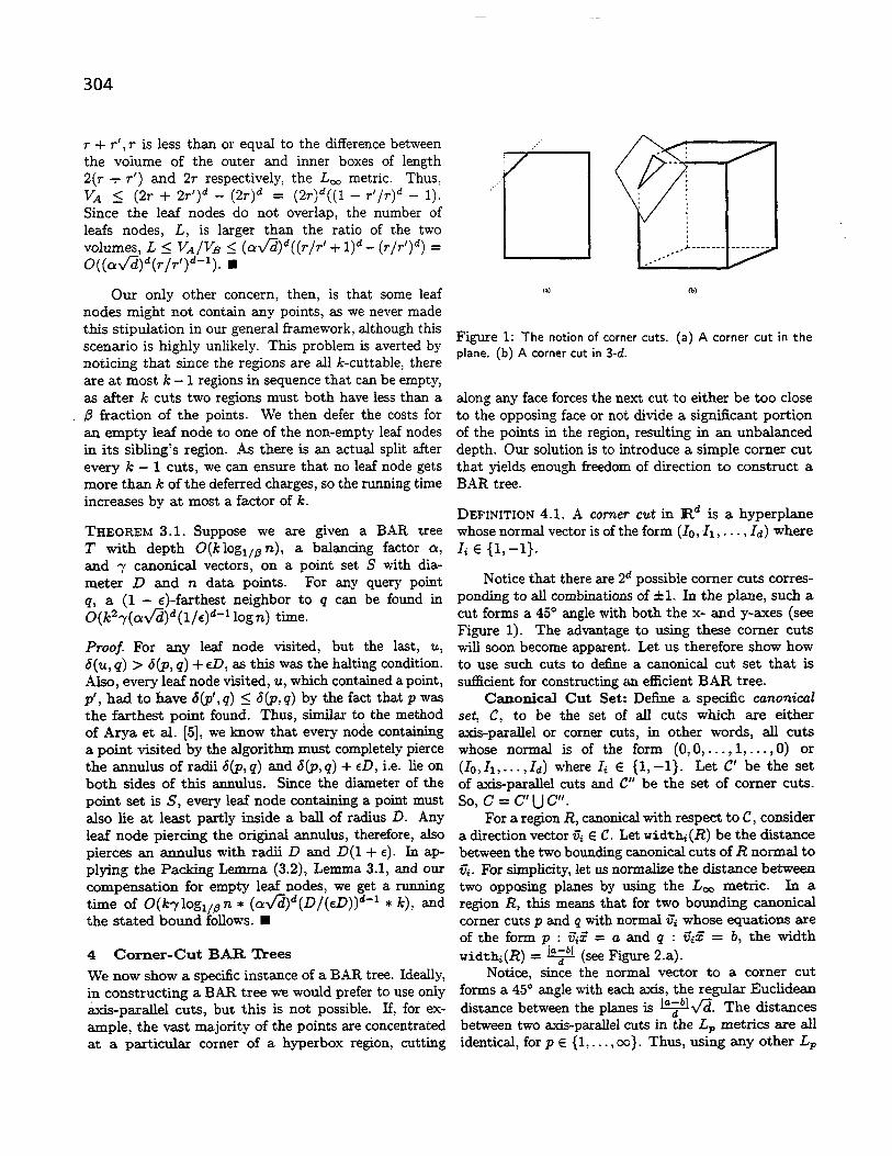
Figure 3: (a) Two cuts 1 and T which divide a region R into subregions Rr, Ii&. and R,r. (b) Pairs of parallel cuts II. rl and 12, rs divide region R into several subregions. The shaded areas are the intersections of the outer regions.

that some other bounding canonical cut, c, in R is no longer a bounding canonical cut in RI, i.e. it is no longer tangential to the new subregion RI. If this is the case, we simply take the bounding canonical cut of RI which is parallel to c to represent part of RI. Therefore, when we refer to canonical cuts of a region, we are always referring to the region’s bounding canonical cuts.

Every corner cut, besides having an opposing corner, also has d neighboring axis-parallel cuts, and d opposing axis-parallel cuts. For a comer cut, c = (&,&, . . . ,&f), let d = (0,. . . ,Ij,.. . ,o) for j E {l,d} be the j-th neighboring cut.

LEMMA 4.1. Suppose we are given a convex polyhedral region R, and two parallel hyperplanes 1 and T intersecting R (see Figure 3.a). We have three (possibly empty) subregions of R lying to the left, middle, and right of the two hyperplanes, respectively, RL, &, and Rr. For any 1 3 @ 1 l/2, either there exists a hyperplane m parallel to 1 and T intersecting R, which divides the region into two subregions both of which have no more than PjRj points or no less than PlRl points lies in either RL or R.7.

Proof. Assume the contrary. Then, we know that 1 Rr 1 < PlRl which implies that I&I + lRr[ 2 PIRI, or else the line 1 would be a suitable choice for m. Similarly, we know that l&l + l&l 1 PIRI. We now continually sweep a hyperplane m from I towards r, let RI and R2 be the two subregions of R to the left and right of m. [RI1 = \RI~ + z for 0 5 z < I&I. This implies that there exists z f (0,. .., I&l} such that IRlJ = PlRl and lR2j = JR1 - PiRl 5 ,8lRl for ,0 2 l/2. Thus, there exists a hyp&plane parallel to I and T which intersects R, and divides R into two regions of size no more than flIR[, contradicting our original assumption. n

In other words, there either is a cut that divides a region into two subregions each with less than a fraction

306

of the original number of points or one of the two outside COROLLARY 4.1. Given a canonical region R, a vector regions has more than this fraction of points. If this v’i E C and a reduction factor 1 > ,8 2 l/2, let b and latter case holds, we call this region the large outer c be the two opposing canonical cuts in R with normal region, lorl,,(R), where 1 and T are the two parallel ci. If shiel&(R) n shiel&(R) = 0, then either a cut hyperplanes. If there exists a dividing cut, m, then exists which divides R into two o-ba,la,nced region Rr loq,(R) = 0. and RZ each with less than PlRl points or one of the

THEOREM 4.1. Suppose we are given a convex region shield regions has more than ,BlRl points.

R, and k pairs of paralle1 hyperplanes (&, ri), i E Proof. Since the two regions do not intersect, we have (1,. . . , k} (see Figure 2.b). For any fi 2 (k - 1)/k the two cuts defining each shield divide R into three (and P 2 l/2), either there exists a hyperplane m regions, as in Lemma 4.1, the size constraints hold. parallel to one of the pairs which divides the region More importantly, by the d&&ion of a &&ld re@on

into two subregions of size less than P/RI or IPI 2 (4.3) and the fact that the two shield regions do not (1 - (1 - p)k)IRj, where P = nf=, 10q,~;(R). intersect, any cut lying between the two regions will

produce two a-balanced. regions. n Proof. Assume that there does not exist a hyperplane m dividing the region into two small subregions. By We refer to the shield region from the above corol- Lemma 4.1, every pair must have a maximal outer lary as the large outer shield, losi(R), where losi (R) = region for R or we would have a dividing hyperplane 0 if a dividing cut exists. Notice, the corollary corres- m. For each pair (Zi, ri), let Pi = lorli,r,.(R) be the ponds to Lemma 4.1, with the added guarantee that large outer region of R for each pair of hyperplanes. the two regions produced from the cut chosen are cr-

If k = 1, we know, from Lemma 4.1, 141 1 PlRl 2 balanced. Furthermore, this corollary may be exten- (1 - (1 - P)k)IR(. By induction, assume the theorem ded to multiple hyperplane directions, i.e., extends The- holds for all values less than k. Recall from set theory orem 4.1. thatfortwosetsAandB, IAnI = jAI+IBI-IAIJBI. Let P’ = nfzt Pi. We know that lP’UPk( 5 lR(. DEFINITION 4.4. For a given canonical region R and a Then, P = P’nPk + IPI 2 (1 - (1 - P)@ - l))iRI + canonical corner cut c, the length, Ien,( is defined

@[RI - IRI = (1 - (1 - P)k)(RI. Th us, it is true for k as as the distance from the cutting hyperplane c to the

well. I associated comer of the bounding hyperbox containing R, i.e., how far into the region does c cut, measured in

There are many corollaries that can be derived from the L, metric. this simple theorem. For example, if the intersection of all the large outer regions is empty and P > (k - 1)/k, Imagine any axis-parallel hyperbox. If we were to a hyperplane cut must exist that divides the region into remove any corner and continue cutting inward, after two subregions of size less than PlRl each as there is no traveling a certain length we would begin to shrink the other alternative location for the points to lie. bounding box of the remaining region, in at least one

of the axis dimensions. After going even a little farther, DEFINITION 4.3. Given an a-balanced canonical region we would begin to &rink the bounding box in every R and a canonical cut c with normal v’i, sweep a cut c’ dimension simultaneously. The instant at which this from the opposing cut towards c, calling the region of happens is the largest the comer cut can possibly be R between these two cuts P, either until P is empty or while guaranteeing that the bounding hyperbox of the just before casp(P) > cy. Notice, if P, is not empty, remaining region is now actually a hypercube. Because then P has maximum aspect ratio. Call the region P, we exploit this property in proving certain regions are the shield region of c in R, shield,(R). one-cuttable, we more formally state and prove this

corollary next. THEOREM 4.2. Given R, c, and c’ as defined above, if shield,(R) # 0 d an we continue sweeping c' towards c, COROLLARY 4.2. For a given canonical region then the region between cand c’ will have anunbala.nced R and a canonica,l corner cut c, Ien, 5 aspect ratio until it becomes empty. maxiec(uidthi(R))(l - l/d). If equality holds,

Proof. Intuitively, if a convex region R starts out fat then hasp(R) = 1.

and in the process of cutting m a constant direction Pmof. Wlog, assume that c = (1,1,. . . , I), i.e., the becomes skinny, continuing in that direction will never upper left hand comer, and the corresponding corner make it fat again. I of the bounding hypercube for R be placed at the

307

origin. This makes the equation of the hyperplane for c, (1, 1,. . . , 1)s = len,(R)d.

Let z = ma.xiec(widthi(R)) be the maximum width between all of the bounding canonical cuts. This must then correspond to a particular pair of axis-parallel cuts. Wlog, assume that they are cl, (l,O,. . . ,O)Z = 0, and its opposing cut br , (1, 0, . . . , 0)Z = z, i.e. the left and right sides.

Now, assume that len,(R) > ~(1 -l/d) = $(d- 1). Let the intersection of hyperplanes c and c1 be the hyperplane c’, (0, 1, 1, . . . , l)Z = len,(R)d. Notice that since c n R and cr n R, c’ n R # 0. However, no point p E R can lie on c’, as (0, 1, 1, . . . , 1)~ 5 z * (d - 1) = $(d - l)(d) < len,(R)d. Thus, c’n R = 0. +*

For the second statement, if len,(R) = ~(1 - l/d) and following a similar argument from above, we know that the distance from every axis-parallel side must also be at length x, or again no point in R can lie on the intersection of the two hyperplanes. n

LEMMA 4.2. For an a-balanced canonical region R and a corner cut c,

rney(widthi(R)) < d(len,(R) + width,(R))

Proof. For simplicity, assume that the corner cut has normal vector, ci = (1, 1, _ _ _ , 1) and the associated comer of the bounding hyperbox is at the origin. The hyperplane equation of the corner cut c is then %E = dlen,(R) and the opposing bounding comer cut has equation v’i5 = d(len,(R) + widt&(R)). Thus, the distance between any two axis-parallel sides of the region and its associated bounding hyperbox must be no more than d(len,(R) ,+ widt&(R)). Since we are using the L, metric, the maximum distance between any two bounding hyperplanes in R must correspond to one of the axis-parallel sides, i.e., a hyperplane on the bounding box, and the result follows (see Figure 4.a). n

LEMMA 4.3. (Corner-Cut Shield Lemma) For an o-balanced canonical region R and a comer cut c E C”, width,(shiel&(R)) 5 len,(R)/(s - l), for a > d.

Proof. Let x = Ien,( P = shiel&(R), y = width,(P), and z = mUZiec(widt&(P)). We kllOW from Lemma 4.2 that z 5 (x + y)d. Since P is the shield region for c, casp(P) = a. Because we are using the L, metric, y is the minimum width in P, implying that zfy = a =$ y = z/a 5 (x + y)d/a. Solving for y, we get y 5 xd/(cy - d) = z/(5 - 1) (see Figure 2.b). m

This lemma is where the main advantage to using comer cuts comes in. If the corner cut is small, i.e., cuts very little of the region, we can make a cut in that

direction very close to this corner cut, in proportion to its size and disregarding the dimensions of the rest of the region entirely.

4.2 k-Cut Existence Theorem. Before we prove that every balanced canonical region is (d + 2)-cuttable, we first describe a few regions that are k-cuttable for k 5 3.

THEOREM 4.3. For p > (d - 1)/d and 01 > 2d, an o-balanced canonical region R is one-cuttable if there exists a corner cut c E C” with opposing cut b such that

1. lenb(R) = maxiec(widt&(R))(l - l/d),

2. len,(R) > maxiec(widthi(R))(l/a).

Proof. Wlog, assume that c = (1, 1, . . . , 1). Let x = maxiec (widthi(R Recall from corollary 4.2, hasp(R) = 1. Now, let us look at the various shield regions for each of the axis-parallel directions, i& E C’, of the neighboring face, bi, of b. If we look at any hyperspace cut along this direction, the region formed towards this neighboring face will always have hasp(R) = 1. This is because of the comer cut b which cuts every neighboring face simultaneously. Therefore, Pi = shieldbi (R) = 0. In the other direction, Qi = shield,<(R), has balanced aspect ratio a, this implies that widt&(R) 5 x/a. We can do this for every one of the axis-parallel directions. We have d pairs of shield regions (Pi, Qi), Vi E (1,. . . , d). From corollary 4.1, this means that for any @ > (d - 1) /d either a one-cut exists or at least (1 - (1 - P)d)lRI > 0 points lies in one of the intersections of the regions. Let us determine which intersection of regions this could be. If it contained any of the Pi regions, the intersection would be empty as Pi is empty, notice the strictly greater than 0 condition.

W

.

Figure 4: (a) The longest side of the bounding box of a given cannonical region has to be shorter than the sum of the length and distance of the corner cuts, i.e. z 5 (I + y)d. (b) An example of a basic one-cuttable region in the plane. Notice that y = z/2 and z 2 z/a

308

Therefore, at least one point must lie in I = n%, &i. Now, let us look at Inc. Notice that len,(R) > z/o, yet in I, widt&(I) <= z/cr,V’i E (1,. . . ,d). The intersection is empty and no points in R can lie in this intersection either. Consequently, there must be a one- cut on R. H

have additional corner cuts. However, with the simple addition of one extra shield cut in one of the d axis- parallel directions, it is not too difficult to see that we can produce a region which is one-cuttable, although we leave the details for the journal version. m

THEOREM 4.4. For CY 2 3d and ,f3 2 d/(d + l), an a-balanced canonical region R is three-cuttable if hasp(R) 5 2.

THEOREM 4.5. For o 2 3d and p 1 d/(d + l), any o-balanced canonical region R is (d -t 2)-cuttable.

Proof. Let z = rnaxiec~ (widthi(R y = miniecl(widthi(R)), and n = IRI. Since b=+(R) = z/y 5 2, z/2 < y. For each axis-parallel direction, Gi, let us End the two shield regions, Pi and &i, associated with the opposing cuts. Wlog, let us look at P;. Notice, that the widt&(Pi) 5 t/a 5 z/4 5 y/2 and the same for &i which implies that Pi n Qi = 0. Since p 2 d/(d + 1) > (d - 1)/d, from C* rollary 4.1, either a dividing cut exists or P = &c, los;(R) # 0. If a dividing cut exists, we are done, as the region is by definition three- cuttable. Otherwise, we know from our corollary that IPI 2 (1-(1-P)d)n 2 (1-(1-d/(d+l))d)n = n/(d+l).

It is quite clear from our construction of P that P corresponds to one of the 2d corners of the bounding hyperbox of R. Wlog, let this be the upper left corner, i.e. the comer whose associated cut is 5i = (1, 1, . . . , 1). Now, since P is not empty, len,(R) 5 widt&(P) 5 z/a. Let PC = shiel&(R) and Pt, = shiel&(R), where b is the opposing cut of c. Because b can be at most the diagonal, len,(R) + width,(R) 2 z/d. Then, since leQ(R) 5 Z/Q, width&R) 2 z(l/d - I/Q. For QC 2 3d, this means width,(R) 2 2z/(r and a cut exists between b and c which creates two a-balanced regions. This means Pt, n PC = 0. Also, from this, we know that Pb n P = 0. Now again, either a dividing cut exists in R in which case we are again finished or at least @n of the points lies in either PC or &. If IPbl _> ,L%, then JR - Pi] < (1 - ,6)n. However, lR - PbI > jPI > n/(d + 1) > (1 - /?)n which implies /PC1 1 ,&z, but /Pbl > @z, a contradiction.

Proof. Let z = rnaxiecl (width?(R)) and y = miniecl (widthi(R If hasp(R) 2 2, we are done as the region is three-cuttable. If not, then there exists at least one axis-parallel direction with width less than z/2 which means that y < z/2 =+ t > 2y. Let i f C’ be the direction corresponding to z, i.e., corresponding to the longest side, and b and c be the two opposing canonical cuts with normal v’i. Since z is large, it is easy to see that shiel&(R) n shiel&(R) # 0. Now look at the losi(R). If losi(R) = 0, then a dividing cut exists in R in direction Gi and R is one-cuttable. Note that in many cases, especially those applications that find k-d trees practical, losi(R) will be empty as there is usually a dividing cut .along the longest direction that produces cr-balanced subregions. Otherwise, wlog, assume shield,(R) is the large outer region. Now, rather than cut at this shield region, we use a cut, c’, in the direction of i7; to create a region R’ where widthc(R) = y. Notice that R 1 R’ > shield,(R), i.e., R’ is larger than the shield region, and if R’ is k-cuttable, then R is (k+ 1)-cuttable. Also, since there are at most d- 1 sides with width greater than y and after every cut we reduce this count by one, after no more than d - 1 cuts we will have an o-balanced canonical region with hasp(R) 5 2, which is three-cuttable. Therefore, any a-balanced canonical region is (d + 2)-cuttable. n

Notice that our scheme generally cuts along the longest axis-parallel side. We can alter this to include searching for one-cuts in the other axis-parallel directions and in so doing mimic the performance of k-d trees. In practice, as k-d trees often appear to perform quite well, the special two-cuttable regions may never have to be used. However, we have the added safety net of using these comer cuts, and in fact even finding ap- propriate one-cuts and two-cuts are quite easy although their existence is diacult to prove. .

THEOREM 4.6. For the given canonical set, C, a BAR tree with depth O(d2 logn) and balancing factor a can be constructed in 0(&m logn) time, where y is the size of the canonical set, here O(2d). This is O(nlogn) for fixed dimensions.

We claim that PC is three-cuttable. First, observe that IR-PC1 5 (l-&z 2 on; thus, if PC is twocuttable then by definition R is three-cuttable. By the Comer- Cut Shield Lemma 4.3, width,(P,) 5 len,(R)/(cr/d - 1) 5 le&(R)/2 + z’ = maxiec(widt&(P,)) < d(len,(P,) + widthc(Pc)) 5 3dlen,(P,)/2. Recall that len,(P,) = lew(R) 5 Z/CX and Q! 2 3d. This means that z’ 5 3dz/(2cr) 5 z/2. Since y 1 z/2, one of two types of regions may be formed. We know that either the bounding box of PC has minimum width z’, in which case PC is one-cuttable, or PC is nearly identical to the region in Theorem 4.3 except that the comers may

Proof. Notice that at any stage, using even the most naive search, the large outer regions of a region R can

be found in O(lRI) t ime, and the shielding regions at each stage can easily be found in O(y) time. Thus, we can find any k-cut of a region R in O(lR1-y) time. Since the depth is bounded, we have the running time as O(kyn log,,p n) time. Noticing that k = O(d) and P = O(dl(d + 1)) =+- 1 g, above stated runrung t~rn~.‘z = o(dlogn)’ we get the

. .

5 Conclusion and Open Problems

In this paper, we introduced the general framework of the BAR tree and described some important applications that may be solved by using this type of tree. We also showed that when the dimensionality is fixed, an (a, @)-BAR tree can be constructed in O(nlogn) time, where n is the number of points in the data set.

These results, however, are only preliminary. There are still many open problems for this new type of data structure. For example, the complexity of the canonical regions (O(2d)), the number of cuts needed to ensure &balance (O(d)), and the maximum a-balance factor (O(d)) are all far from optimal and could with more careful analysis be significantly dropped, perhaps by choosing a different canonical set entirely.

References

PI

PI

[31

PI

171

PI

PI

P. K. AGARWAL, E. F. GROVE, T. M. MURALI, AND J. S. VITTER, Binary space partitions for fat rectangles, in Proc. 37th Annu. IEEE Sympos. Found. Comput. Sci., Oct. 1996, pp. 482491. P. K. AGARWAL, M. KATZ, AND M. SHARIR, Comput- ing depth orders for fat objects and related problems, Comput. Geom. Theory Appl., 5 (1995), pp. 187-206. W. G. AREF AND H. SAMET, Perspective viewing’ of objects represented by octrees, Comput. Graph. Forum, 14 (1995), pp. 59-66. also University of Maryland Computer Science TR-2757. S. ARYA AND D. M. MOUNT, Approzimate mnge searching, in Proc. 11th Annu. ACM Sympos. Comput. Geom., 1995, pp. 172-181. S. ARYA, D. M. MOU&T, N. S. NETANYAHU, R. SILVERMAN, AND A’. WV, An optimal algorithm for approzimate nearest neighbor searching, in Proc. 5th ACM-SIAM Sympos. Discrete Algorithms, 1994, pp. 573-582. J. L. BENTLEY, Multidimensional binary search trees used for associative senrching, Commun. ACM, 18 (1975), pp. 509-517. -, K-d trees for semidynamic point sets, in Proc. 6th Axmu. ACM Sympos. Comput. Geom., 1990, pp. 187-197. P. B. CALLAHAN AND S. R. KOSARAJU, Algorithms for dynamic closest-pair and n-body potential fields, in Proc. 6th ACM-SIAM Sympos. Discrete Algorithms, 1995, pp. 263-272. P. B. CALLAHAN AND S. R. KOSARAJU, A decomposition of multidimensional point sets with applications to k-nearest-neighbors and n-body potential fields, J. ACM, 42 (1995), pp. 67-90.

WI

Pll

P4

[I31

[I41

P51

WI

[171

[W

WI

PO1

Pll

WI

1231

1241

[251

[261

[271

WI

309

H. H. CHEN AND T. S. HUANG, A survey of construction and manipulation of octrees, Comput. Vision Graph. Image Process., 43 (1988), pp. 409431. N. CHIN AND S. FEINER, Near real-time shadow gen’er- ation using BSP trees, in Proc. SIGGRAPH ‘89, New York, Aug. 1989, ACM SIGGRAPH, pp. 99-106. M. DE BERG, Linear size binary space partitions foT fat objects, in Proc. 3rd Annu. European Sympos. Algorithms, vol. 979 of Lecture Notes Comput. Sci., Springer-Verlag, 1995, pp. 252-263. C. A. DUNCAN, M. T. GOODRICH, AND S. G. KOBOR- UOV, Balanced aspect ratio trees and their use for drawing very large graphs, in Sixth Symposium on Graph Drawing, to be published in 1998. A. EFRAT AND M. SHARIR, On the completity of the union of fat objects in the plane, in Proc. 13th Annu. ACM Sympos. Comput. Geom., 1997, pp. 104-112. R. A. FINKEL AND J. L. BENTLEY, Quad trees: a data structure for retrieval on composite keys, Acta Inform., 4 (1974), pp. 1-9. H. FUCHS, Z. M. KEDEM, AND B. NAYLOR, On visible surface generation by a priori tree structures, Comput. Graph., 14 (1980), pp. 124-133. Proc. SIGGRAPH ‘80. A. HENRICH, Improving the performance of multi- dimensional access strwtures based on kd-tiees, in Proc. 12th IEEE Intl. Conf. on Data Engineering, 1996, pp. 68-74. C. JACKINS AND S. L. TANIMOTO, Ott-trees and their use in representing 3-d objects, Comput. Graph. Image Process., 14 (1980), pp. 249-270. M. J. KATZ, 3-D vertical my shooting and 2-D point enclosure, range searching, and arc shooting amidst convez fat objects, Comput. Geom. Theory Appl. to appear. J. MATOU~EK, J. PACH, M. SHARIR, S. SIFRONY, AND E. WELZL, Fat triangles determine linearly many holes, SIAM J. Comput., 23 (1994), pp. 154-169. M. H. OVERMAR~ AND A. F. VAN DER STAPPEN, Range searching and point location among fat objects, J. Algorithms, 21 (1996), pp. 629-656. M. H. OVERMAR~ AND J. VAN LEEUWEN, Dynamic multi-dimensional data structures based on quad- and k-d trees, Acta Inform., 17 (1982), pp. 267-285. M. S. PATERSON AND F. F. YAO, Eficient binary space partitions for hidden-surface removal and solid modeling, Discrete Comput. Geom., 5 (1990), pp. 485- 503. -, Optimal binary space partitions for orthogonal objects, J. Algorithms, 13 (1992), pp. 99-113. H. SAMET, The quadtree and related hiemmhicul data structures, ACM Comput. Surv., 16 (1984). -, An overview of quadtrees, octrees, and related hiemrchical data stnxtures, in Theoretical Foundations of Computer Graphics and CAD, R. A. Eaxnshaw, ed., vol. 40 of NATO ASI Series F, SpringerlVerlag, Berlin, West Germany, 1988, pp. 51-68. -, The Design and Analysis of Spatial Data Struc- tures, Addison-Wesley, Reading, MA, 1990. E. TORRES, Optimization of the binary space partition algorithm (BSP) for the visualization of dynamic scenes, in Eurographics ‘90, North-Holland, 1990, pp. 507-518.

balanced aspect ratio trees:: combining the …goodrich/pubs/bar-soda.pdfbalanced aspect ratio...

Documents