band-dominated operators and the stable ... - math…
TRANSCRIPT

The Pennsylvania State University
The Graduate School
Department of Mathematics
BAND-DOMINATED OPERATORS AND THE STABLE
HIGSON CORONA
A Dissertation in
Mathematics
by
Rufus Willett
c© 2009 Rufus Willett
Submitted in Partial Fulfillmentof the Requirements
for the Degree of
Doctor of Philosophy
August 2009

ii
The dissertation of Rufus Willett was reviewed and approved* by the following:
John RoeProfessor of MathematicsDissertation AdviserChair of CommitteeHead of the Department of Mathematics
Paul BaumEvan Pugh Professor of Mathematics
Nathanial BrownAssociate Professor of Mathematics
Nigel HigsonEvan Pugh Professor of Mathematics
Donald SchneiderDistinguished Professor of Astronomy and Astrophysics
*Signatures are on file in the Graduate School.
iii
Abstract
Band-dominated operators form a class of bounded operators on l2(Zn) that have
been studied in various forms throughout the twentieth century, and arise naturally in
many areas of mathematics. One aspect of work of V.S. Rabinovich, S. Roch and B.
Silbermann on this class of operators has been a workable criterion for whether or not
such an operator has the Fredholm property. Their work suggests in particular a natural
index problem for such operators, which was solved for the case of operators on l2(Z) by
Rabinovich, Roch and J. Roe. This dissertation proves a partial generalization of this
result to band-dominated operators with slowly oscillating coefficients on l2(Zn), using
the stable Higson corona of H. Emerson and R. Meyer. Part of the interest of this result
is that it highlights a difference between the ‘slowly oscillating’ and general cases that
only appears in dimensions higher than one.
This stable Higson corona was introduced by Emerson and Meyer in the last five
years in the course of their work on the Baum-Connes and Novikov conjectures. This
dissertation gives simpler proofs of some of the properties used in the proof of the index
theorem mentioned above. These results are also of independent interest insofar as they
reprove certain results on the Baum-Connes and coarse Baum-Connes conjectures.

iv
Table of Contents
List of Figures . . . . . . . . . . . . . . . . . . . . . . . . . . . . . . . . . . . . . vi
Acknowledgments . . . . . . . . . . . . . . . . . . . . . . . . . . . . . . . . . . . vii
Chapter 1. Introduction . . . . . . . . . . . . . . . . . . . . . . . . . . . . . . . . 1
Chapter 2. Band-dominated operators on Zn . . . . . . . . . . . . . . . . . . . . 12
2.1 Definition and examples . . . . . . . . . . . . . . . . . . . . . . . . . 12
2.2 Limit operators and the Fredholm property . . . . . . . . . . . . . . 24
2.3 An index theorem for the case n = 1 . . . . . . . . . . . . . . . . . . 37
2.4 Problems with extending this to Zn . . . . . . . . . . . . . . . . . . 44
Chapter 3. Generalizations and special cases . . . . . . . . . . . . . . . . . . . . 49
3.1 The relevance of crossed product algebras . . . . . . . . . . . . . . . 52
3.2 Special cases . . . . . . . . . . . . . . . . . . . . . . . . . . . . . . . 57
3.3 Example: slowly oscillating functions and the Higson corona . . . . . 60
3.4 Example: pseudodifferential operators on the n-torus . . . . . . . . . 64
3.5 Example: the visibility boundary of a CAT (0) space . . . . . . . . . 69
3.6 Example: the Gromov boundary of a hyperbolic group . . . . . . . . 72
Chapter 4. The stable Higson corona . . . . . . . . . . . . . . . . . . . . . . . . 77
4.1 The ‘Higson conjecture’ . . . . . . . . . . . . . . . . . . . . . . . . . 78
4.2 The ‘stable Higson conjecture’ and coarse co-assembly map . . . . . 82

v
4.3 Homological properties of the stable Higson corona . . . . . . . . . . 87
4.4 Geometric boundaries . . . . . . . . . . . . . . . . . . . . . . . . . . 108
4.5 Open cones . . . . . . . . . . . . . . . . . . . . . . . . . . . . . . . . 110
4.6 CAT (0) spaces . . . . . . . . . . . . . . . . . . . . . . . . . . . . . . 114
4.7 Gromov hyperbolic spaces . . . . . . . . . . . . . . . . . . . . . . . . 117
Chapter 5. An index theorem for Zn, after Deundyak and Shteinberg . . . . . . 133
Chapter 6. Two applications of bivariant K-theory . . . . . . . . . . . . . . . . . 141
6.1 Asymptotic morphisms . . . . . . . . . . . . . . . . . . . . . . . . . . 141
6.2 The Baum-Connes conjecture . . . . . . . . . . . . . . . . . . . . . . 154
Appendix A. Functors on coarse categories . . . . . . . . . . . . . . . . . . . . . 164
Appendix B. Crossed products and exact groups . . . . . . . . . . . . . . . . . . 174
References . . . . . . . . . . . . . . . . . . . . . . . . . . . . . . . . . . . . . . . . 183

vi
List of Figures
1.1 Schematic of an order zero pseudodifferential operator on the circle . . . 2
1.2 Matricial picture of a class of operators on l2(Z) . . . . . . . . . . . . . 5
1.3 The spherical compactification of Z . . . . . . . . . . . . . . . . . . . . . 6
2.1 Schematic of a band operator on l2(Z) . . . . . . . . . . . . . . . . . . . 14
2.2 Idea of a limit operator . . . . . . . . . . . . . . . . . . . . . . . . . . . 28

vii
Acknowledgments
I would like to thank Mrinal Raghupathi and Guoliang Yu for helpful comments
on aspects of the current work after a talk given at Vanderbilt University. I would also
like to thank Steffen Roch for interesting discussions and showing me the paper [15].
It is a pleasure to thank all of the members of my committee for their support,
comments and encouragement. The mathematical members have also all provided a great
deal of inspiration through their teaching, conversation and writing. As importantly, they
have created a very enjoyable atmosphere in the Geometric Functional Analysis group at
Penn State. Conversations with many of the students in this group, in particular Uuye
Otgonbayar, also permeate this thesis; thanks to all.
In addition to the comments above, John Roe encouraged me to come to Penn
State in the first place, and was extremely welcoming once I arrived. His support, and
patience, have been more than appreciated throughout.
Further back, it is due to the influence of Sue Barnes, Clive Sutton and in partic-
ular Glenys Luke that I am in mathematics. I am deeply grateful for their instruction,
which constantly informs my own approach.
Finally, I would very sincerely like to thank my family and friends in the UK, and
in particular my parents, for continuing to support me and welcome me back, despite
the mildly quixotic decision to place myself in a small town halfway around the world :)
.

1
Chapter 1
Introduction
A classical index theorem
In order to motivate the rest of this piece, we start by discussing a slight variation
of the Gohberg-Krein index theorem. Chapter 7 of [16] is a good reference for what follows.
Let l2(Z) be the Hilbert space of square-summable maps from Z to C, equipped
with the fixed orthonormal basis δn : n ∈ Z. A bounded linear operator T on l2(Z)
can be uniquely represented as a matrix with entries indexed by Z × Z: the (n,m)th
entry is 〈Tδm, δn〉, just as in the case of a linear operator on a finite-dimensional vector
space.
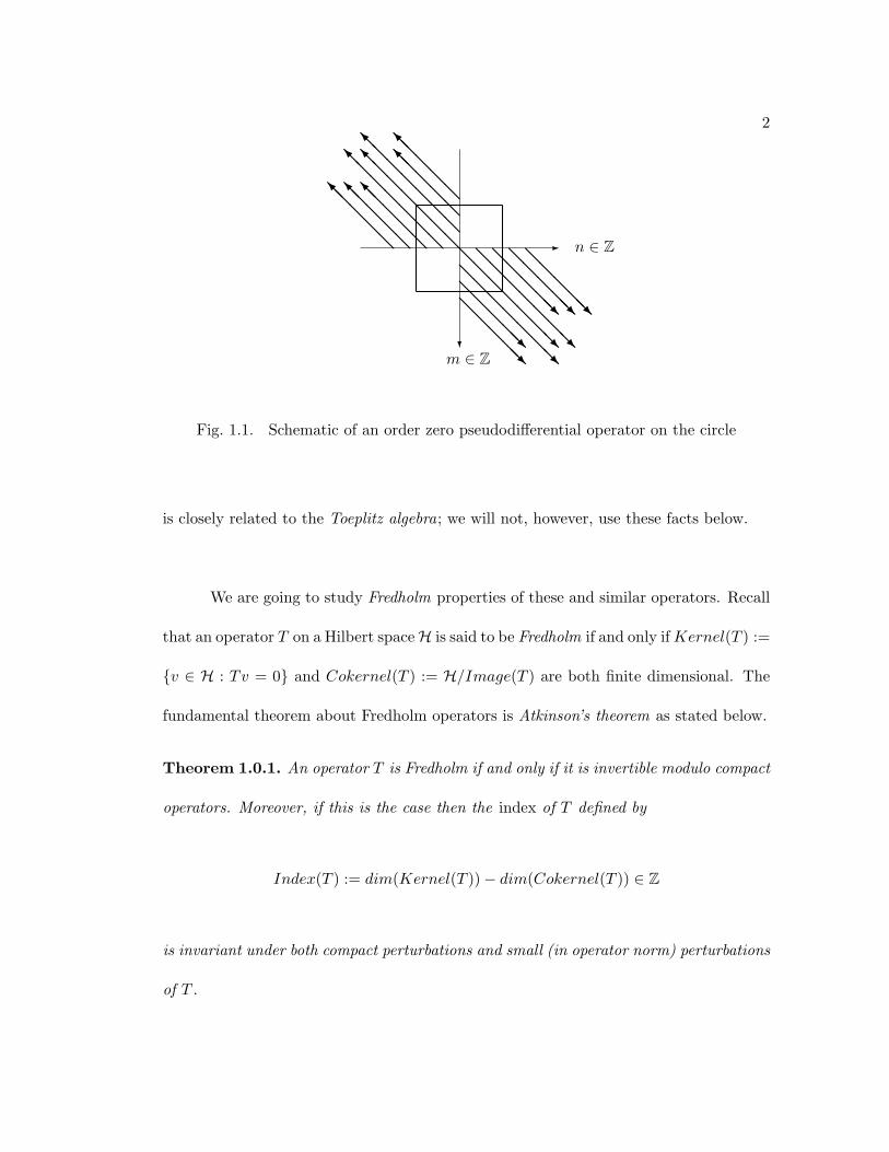
There are many interesting classes of operators that can be described in terms of
such a matricial representation. For example, figure 1.1 below represents an operator
where
• the sequence of matrix coefficients along each diagonal arrow converges to some
complex number at infinity;
• there are only finitely many arrows;
• all other matrix coefficients outside the central box are zero.
Such operators form a ∗-algebra, with norm closure a C∗-algebra denoted Ψ0(T).
It is in fact the C∗-algebra of order zero pseudodifferential operators on the circle T, and
2
-
?m ∈ Z
n ∈ Z@
@@
@@
@@R
@@
@@
@@
@R
@@
@@@R
@@
@@@R
@@
@@
@@
@R
@@
@@@R
@@
@@@R
@@
@@@R
@@
@@
@@
@I
@@
@@
@@
@I
@@
@@
@I
@@
@@
@I
@@
@@
@@
@I
@@
@@
@I
@@
@@
@I
@@
@@
@I
Fig. 1.1. Schematic of an order zero pseudodifferential operator on the circle
is closely related to the Toeplitz algebra; we will not, however, use these facts below.
We are going to study Fredholm properties of these and similar operators. Recall
that an operator T on a Hilbert spaceH is said to be Fredholm if and only ifKernel(T ) :=
v ∈ H : Tv = 0 and Cokernel(T ) := H/Image(T ) are both finite dimensional. The
fundamental theorem about Fredholm operators is Atkinson’s theorem as stated below.
Theorem 1.0.1. An operator T is Fredholm if and only if it is invertible modulo compact
operators. Moreover, if this is the case then the index of T defined by
Index(T ) := dim(Kernel(T ))− dim(Cokernel(T )) ∈ Z
is invariant under both compact perturbations and small (in operator norm) perturbations
of T .
3
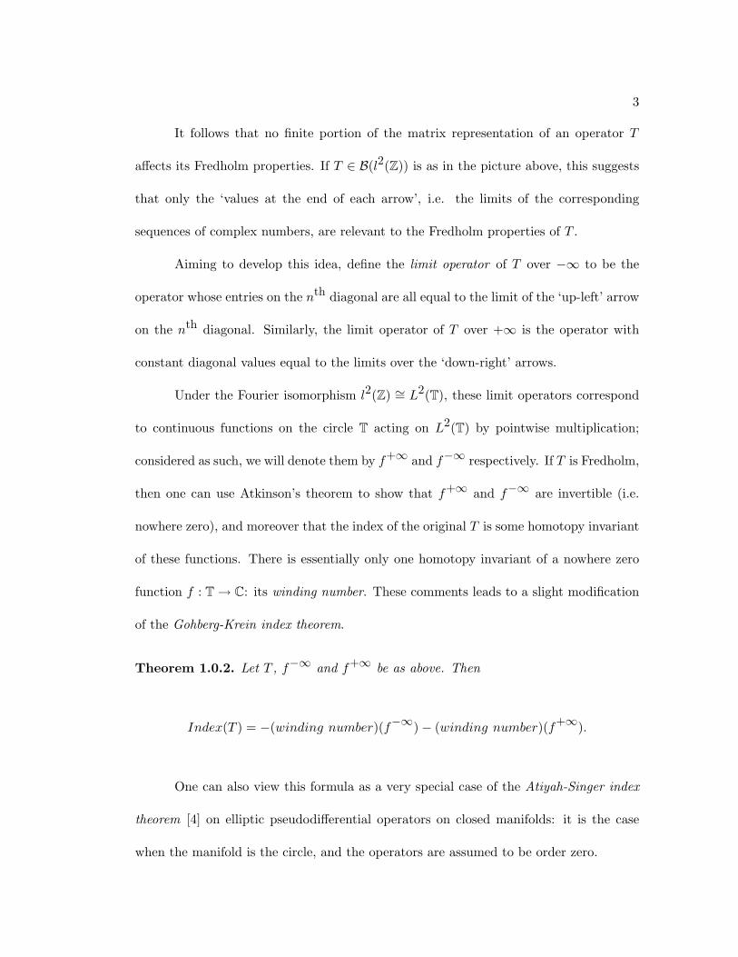
It follows that no finite portion of the matrix representation of an operator T
affects its Fredholm properties. If T ∈ B(l2(Z)) is as in the picture above, this suggests
that only the ‘values at the end of each arrow’, i.e. the limits of the corresponding
sequences of complex numbers, are relevant to the Fredholm properties of T .
Aiming to develop this idea, define the limit operator of T over −∞ to be the
operator whose entries on the nth diagonal are all equal to the limit of the ‘up-left’ arrow
on the nth diagonal. Similarly, the limit operator of T over +∞ is the operator with
constant diagonal values equal to the limits over the ‘down-right’ arrows.
Under the Fourier isomorphism l2(Z) ∼= L2(T), these limit operators correspond
to continuous functions on the circle T acting on L2(T) by pointwise multiplication;
considered as such, we will denote them by f+∞ and f−∞ respectively. If T is Fredholm,
then one can use Atkinson’s theorem to show that f+∞ and f−∞ are invertible (i.e.
nowhere zero), and moreover that the index of the original T is some homotopy invariant
of these functions. There is essentially only one homotopy invariant of a nowhere zero
function f : T→ C: its winding number. These comments leads to a slight modification
of the Gohberg-Krein index theorem.
Theorem 1.0.2. Let T , f−∞ and f+∞ be as above. Then
Index(T ) = −(winding number)(f−∞)− (winding number)(f+∞).
One can also view this formula as a very special case of the Atiyah-Singer index
theorem [4] on elliptic pseudodifferential operators on closed manifolds: it is the case
when the manifold is the circle, and the operators are assumed to be order zero.

4
K-theory
A natural way to prove the index theorem of the previous section is to use K-
theory. A good introductory reference is [67].
The discussion above can be extended to show the existence of a short exact
sequence of C∗-algebras
0 // K(l2(Z)) // Ψ0(T)σ // C(T)⊕ C(T) // 0 ;
this is essentially a theorem of L. A. Coburn. Associated to any such sequence is a
six-term exact sequence of K-theory groups
K0(K(l2(Z))) // K0(Ψ0(T)) // K0(C(T)⊕ C(T))
K1(C(T)⊕ C(T))
Ind
OO
K1(Ψ0(T))oo K1(K(l2(Z)))oo
.
If T ∈ Ψ0(Tn) is a Fredholm operator, then its image under the symbol map σ is
invertible, so defines a class [σ(T )] in K1(C(T)⊕C(T)). The general theory implies that
the index of T depends only on the K-theory class [σ(T )], and in fact that the map
Ind : K1(C(T)⊕ C(T))→ K0(K(l2(Z))) ∼= Z
form the six term exact sequence above sends [σ(T )] to Index(T ). As one can compute
that the group K1(C(T) ⊕ C(T)) is isomorphic to Z ⊕ Z, to prove the theorem in the
previous section it suffices to check that it is true on a pair of simple generators.

5
Generalizations and compactifications
The main motivation for this thesis is the work of V.S. Rabinovich, S. Roch
and B. Silbermann on Fredholm theory for band-dominated operators. Band-dominated
operators on l2(Z) constitute a very wide-ranging generalization of the operators in
Ψ0(T) looked at above: they are norm limits of operators whose matrix coefficients are
supported within a pair of diagonal lines like those shown in figure 1.2 below. There are
many interesting examples of band-dominated operators in operator theory, and they
also play a major role in coarse geometry and index theory; see examples 2.1.3 and 2.1.8
below, as well as [56], [63].
-
?m ∈ Z
n ∈ Z
@@
@@
@@
@@
@@
@@
@@
@@
@@
@@
@@
@@
Fig. 1.2. Matricial picture of a class of operators on l2(Z)
There is a notion of ‘limit operator’ for general band-dominated operators, which
was used by Rabinovich, Roch and Silbermann to give a criterion for Fredholmness.
As general band-dominated operators can have very complicated behavior along each

6
diagonal, however, one needs much more than the two point set −∞,+∞ of ‘directions
at infinity’ to coherently organize the limit operators that arise.
To see how to define such generalized limit operators, note that the two points
−∞,+∞ define a compactification of Z as in figure 1.3 below.
q qq qq qq qq qq qq qq qq qq rr−∞ +∞Z -
Fig. 1.3. The spherical compactification of Z
It can be thought of as attaching a copy of the zero-dimensional sphere to Z, and is
called the spherical compactification.
To consider more general ‘directions at infinity’ one can use larger compactifica-
tions of Z; the more complicated the class of diagonals allowed, the more complicated
the necessary compactification. If for example all band-dominated operators are consid-
ered, so all bounded functions are to be allowed as diagonals, one needs the Stone-Cech
compactification of Z to organize all the limit operators. This is the largest possible
compactification. If one puts some conditions on the behavior of the diagonals, smaller
compactifications can be used; one of the simplest of these is the spherical compactifica-
tion considered above. We will also consider band-dominated operators on more general
discrete groups in what follows. Here geometric conditions on the groups lead to limit
operators organized by, for example, the Gromov boundary of a hyperbolic group.

7
One of the most important classes of diagonals considered in the work below
consists of so-called slowly oscillating functions. These are functions whose modulus of
continuity decays to zero at infinity, such as n 7→ sin(√|n|) on Z. The corresponding
class of operators is particularly tractable, and has been studied by Rabinovich, Roch
and Silbermann, and others. The relevant compactification for the study of their limit
operators is the Higson compactification, denoted ∂hZ, which was introduced by N. Hig-
son in the context of index theory [35]. V.M. Deundyak and B.Y. Shteinberg announced
an index theorem for this class of operators in [15]; one of our main results is a new proof
of this theorem, stated as 5.0.1, 6.1.6 and 6.1.10 below.
The stable Higson corona and Baum-Connes conjecture
A K-theoretic approach to the index theorem of Deundyak and Shteinberg leads
one to study the K-group K1(∂hΓ). Unfortunately, this is known to be a very compli-
cated object thanks to the work of J. Keesling [47], and A. Dranishnikov and S. Ferry
[17].
An attempt to get a grasp on the part of this group that is important for index
theory led us to study the stable Higson corona of H. Emerson and R. Meyer [24] [22];
this object forms the second major motivation for the work below. As it happens, the
stable Higson corona has K-theoretic properties that allow us to prove the index theorem
5.0.1 we are aiming for.
There is much more to say here, however. The work of Keesling, Dranishnikov
and Ferry cited above was motivated by connections of the Higson corona to the Novikov

8
conjecture in manifold theory [25], which predicts homotopy invariance of higher signa-
tures. On the other hand, Emerson and Meyer introduced the stable Higson corona for
its connection to the Baum-Connes conjecture [5]. This deep conjecture has a variety
of applications in topology, geometry and representation theory; in particular it implies
the Novikov conjecture.
The properties of the stable Higson corona that we use to prove theorem 5.0.1 are
shown by Emerson and Meyer in [22] using some fairly serious machinery. In an attempt
to give a simpler proof of these properties, and following a well-trodden route [44] [40] [41]
[39], we were led to study the stable Higson corona from a ‘homological’ point of view.
The main results here are theorems 4.3.12 and 4.3.13, which give homotopy invariance
properties of the stable Higson corona and some associated constructions.
These are used to reprove some results of Emerson and Meyer on groups of non-
positive curvature, in what we hope is a more elementary manner.
Organisation of this piece
Chapter 2 introduces band-dominated operators on Zn. In particular, we sketch
proofs of the results of V.S. Rabinovich, S. Roch and B. Silbermann on Fredholmness,
and the index theorem of Rabinovich, Roch and J. Roe which applies in the case n = 1.
The last section of the chapter details some issues that arise when trying to extend this
proof to higher dimensions; these help to motivate the piece as a whole.
Chapter 3 starts by enlarging the class of groups under consideration to that of
exact groups. In section 3.1 we extend some comments from section 4 of [65] to give

9
a proof of the basic Fredholmness properties of the corresponding classes of operators.
This uses some machinery associated to crossed product C∗-algebras. This section sug-
gests associating an index problem to any equivariant boundary of an exact group, as
is made explicit in section 3.2. The rest of the chapter is devoted to discussing some
examples, including those associated to operators with slowly oscillating coefficients.
Chapter 4 opens with a discussion of the Higson corona. The connections of this
object with the Novikov conjecture are summarized for the reader’s convenience in sec-
tion 4.1. The analogous results of H. Emerson and R. Meyer for the stable Higson corona
are then looked at in section 4.2, where we also summarize some connections between the
two approaches. Section 4.3 proves certain homological properties of the stable Higson
corona; the main results are 4.3.12 and 4.3.13 on homotopy invariance. The remaining
sections use these homological properties to study some examples.
Chapter 5 contains most of the proof of theorem the index theorem 5.0.1 of V.M.
Deundyak and B.Y. Shteinberg. The techniques involving crossed products from chap-
ter 3 as well as some simple cases of the computations from chapter 4 are important here.
Chapter 6 is split into two distinct sections. Section 6.1 completes the proof of
theorem 5.0.1 using asymptotic morphisms, and also provides two relatively concrete
restatements in theorems 6.1.6 and 6.1.10. Section 6.2 uses known cases of the Baum-
Connes conjecture to prove isomorphisms in K-theory that would be useful for extending

10
our index-theoretic results to a larger class of groups.
There are also two appendices. Appendix A sets out some necessary background
on coarse categories, which provides the framework for much of chapter 4. Appendix B
briefly discusses the class of exact groups and some results we need on crossed product
C∗-algebras.
Future directions
• There are a lot more groups to study in detail. It should be interesting to look
at connections between the comments on hyperbolic groups in this piece and work
of H. Emerson and M. Jury. The papers of Jury were pointed out to me by
M. Raghupathi, who suggested that concrete index theorems of some interest to
operator theorists may be possible in this direction.
• G. Yu has suggested using the techniques of chapter 4 combined with the fact
that an a-T-menable group acts ‘nicely’ on a Hilbert space (which is CAT (0), but
not proper) may allow one to get results on this class of groups. This would not
yield any new results on the Baum-Connes conjecture - see the deep work of N.
Higson and G. Kasparov [37] - but there may (this is very tenuous currently!) be
connections with the stable Borel conjecture via [33].
• The comments on crossed products in remarks B.3 suggest some interesting ques-
tions here. It seems that they may be connected to the important question as to

11
whether the uniform boundedness condition from corollary 2.2.11 is really neces-
sary.
• It is a major hole in the work below that it only applies to the case of band-
dominated operators on Zn with slowly oscillating coefficients. An index theorem
that worked for band-dominated operators with arbitrary coefficients would prob-
ably not be very computable in general, but seems likely to be of theoretical inter-
est. Note, however, that remark 6.1.9 below suggests that new techniques would
be needed in the proof of such a theorem; I once thought a KK-theoretic approach
might be feasible here, but unfortunately have no ideas along this line currently.

12
Chapter 2
Band-dominated operators on Zn
2.1 Definition and examples
In this section, we approach our central object of study - band-dominated opera-
tors on Zn - from two different directions: operator theoretic, and coarse geometric.
From the operator theory point of view, band-dominated operators are formed
from the following two natural classes of bounded operators on l2(Zn):
• One may consider l∞(Zn) as a subalgebra of B(l2(Zn)), with f ∈ l∞(Zn) acting
by pointwise multiplication. In other words, f acts on elements of the standard
orthonormal basis of l2(Zn) by
f : δm 7→ f(m)δm.
Throughout this piece we abuse notation by writing f for both a function and the
corresponding multiplication operator.
• If m is an element of Zn, we denote by Um the corresponding unitary (left) shift
operator, which is defined on basis vectors by
Um : δl 7→ δm+l.

13
Definition 2.1.1. A band operator is a sum
∑m∈Zn
fmUm (2.1)
where each fm is an element of l∞(Zn) and only finitely many fm are non-zero. A
band-dominated operator is an operator norm limit of band operators.
Note moreover that the band operators form a ∗-subalgebra of B(l2(Zn)), whence
the band-dominated operators form a C∗-algebra. The C∗-algebra of all band-dominated
operators will be denoted C∗u
(|Zn|).
The notation ‘C∗u
(|Zn|)’ comes from the coarse geometric approach to band-
dominated operators, and will be explained after lemma 2.1.7 below.
Remarks 2.1.2. 1. A representation as in line (2.1) is unique. Indeed, any operator
in B(l2(Zn)) can be uniquely (formally) represented in this way, as long as one
allows infinitely many non-zero summands. To see this, note that a representation
of the form (2.1) uniquely determines, and is uniquely determined by, the matrix
coefficients of an operator T ∈ B(l2(Zn)) via the formula
fm(l) = 〈Tδm+l, δl〉. (2.2)
Note that infinite sums of the form (2.1) need not converge (even in the weak
operator topology), however: see part (2) of counterexamples 2.1.4 below.
2. As briefly discussed in the introduction, the name ‘band operator’ comes from
the matrix representation of such an operator on l2(Z). With respect to this

14
representation, a band-operator is one with matrix coefficients supported within a
pair of diagonal lines like those shown in figure 2.1 below (which is the same as
figure 1.2, but repeated for the reader’s convenience).
-
?l ∈ Z
k ∈ Z
@@
@@
@@
@@
@@
@@
@@
@@
@@
@@
@@
@@
Fig. 2.1. Schematic of a band operator on l2(Z)
In this picture, the mth diagonal (i.e. the one m places above the main diagonal)
is the function fm that appears in a representation as in line (2.1). For this reason,
we often call the elements fm in a representation as in line (2.1) above the diagonals
of T .
The class of band-dominated operators on Zn includes many classical examples
from operator theory, operator algebras, and geometric analysis; before continuing, we
will discuss some of these below.

15
Examples 2.1.3. 1. Amongst the simplest band operators are finite sums
∑m∈Zn
λmUm (2.3)
where each λm is a scalar. Such operators are often said to be constant down the
diagonals. They can be thought of as elements of the group algebra C[Zn] acting by
convolution, or (under Fourier transform) as operators of pointwise multiplication
by trigonometric polynomials on L2(Tn). Thus the norm closure of the ∗-algebra of
such operators can be thought of as either C∗r
(Zn), the reduced group C∗-algebra
of Zn, or C(Tn), the continuous functions on the n-torus. It follows from the theory
of Cesaro summation of Fourier series that this C∗-algebra consists precisely of the
band-dominated algebras that are constant down diagonals, i.e. band-dominated
operators of the form in line (2.3) above where the sum is not necessarily finite.
2. Let P ∈ B(l2(Z)) be the orthogonal projection onto the closed span of δn : n ≥ 0.
Let f be an element of C(T), thought of as a band-dominated operator which is
constant down diagonals as in the previous example. The operator PfP is then
band-dominated and called the Toeplitz operator with symbol f . The C∗-algebra
generated by all such operators is the Toeplitz algebra. For a good introduction to
these objects and this algebra, see chapter 7 of [16].
3. From another point of view, the image of P is the Hardy space H2(S1), which
consists of those functions in L2(S1) ∼= l2(Z) that have a (unique) extension to a
holomorphic function on the open unit disc in C.

16
More generally (see [14] and appendix B in [34]), let Pn ∈ B(l2(Zn)) be the or-
thogonal projection onto the closed span of
δm=(m1,...,mn) ∈ l2(Zn) : mi ≥ 0 for all i = 1, ..., n.
Let S2n−1 be the unit sphere in Cn. There is a unitary isomorphism between
l2(Zn) and L2(S2n−1) defined by sending δm=(m1,...,mn) to the monomial
z = (z1, ..., zn) 7→zm := z
m11 · · · zmn
n
V olume(S2n−1). (2.4)
The image of Pn can be identified with H2(S2n−1), the elements of L2(S2n−1)
that have a (unique) extension to a function holomorphic on the open unit ball in
Cn.
Let f ∈ C(S2n−1) act on L2(Zn) by pointwise multiplication. The operator PnfPn
is called a (higher dimensional) Toeplitz operator. As f can be written as a norm
limit of linear combinations of the monomials in line (2.4) above as m ranges over
Zn, PnfPn is band-dominated. These Toeplitz operators are (special cases of) the
operators whose Fredholm properties were studied by Venugopalkrishna in [72].
4. Another case of particular interest is given by pseudodifferential operators on the n-
torus, Tn. These correspond under Fourier transform to band-dominated operators
on Zn whose diagonals (the fm in line (2.1) above) have ‘especially good behavior
at infinity’. See section 3.4 below for details, and section 5 of [4] for an overview
of pseudodifferential operators on more general closed manifolds .

17
5. Many other very interesting classes of band-dominated operators are looked at in
chapters 3, 4 and 5 of [56], and we refer the reader here for further examples.
Some of these (operators of Wiener type, pseudodifference operators,...) fit into the
framework used in this piece.
Counterexamples 2.1.4. 1. It is perhaps worth pointing out that not every operator
in B(l2(Zn)) is band-dominated! For example, consider the operator
T =12
+∑
m∈Z\0
12πim
Um.
This defines a bounded operator on (l2(Z)): it corresponds under Fourier transform
to pointwise multiplication by the descent of the floor function x 7→ bxc from R
to T = R/Z. T is constant down diagonals, so part (1) of examples 2.1.3 implies
that if it were band-dominated, then the (descent of the) floor function would be
continuous on T. As this is not the case, T is not band-dominated.
2. We have seen in part (1) of remarks 2.1.2 that any T ∈ B(l2(Zn)) can be uniquely
formally represented by a sum as in line (2.1). Such a sum need not converge
to T , however, even in the weak operator topology, and even if the original T is
band-dominated.
Indeed, if (fn) is a sequence in C(T) (considered as operators on l2(Z) via part (1)
of examples 2.1.3) that converges to some f ∈ C(T) in the weak operator topology,
then the fn (considered as functions) converge pointwise to f . Hence if f ∈ C(T)
is such that the partial sums of the expression in line (2.1) above converge in the

18
weak operator topology to f , then f is the pointwise limit of the partial sums in its
Fourier series. There are, however, examples of functions f ∈ C(T) for which this
is known to be false; to see existence of such, one can for example use the Baire
category theorem.
We will also study band-dominated operators with a somewhat wider range of
‘matrix coefficients’.
In order to define these, fix a separable (possibly finite-dimensional) Hilbert space
H. Let K(H) denote the C∗-algebra of compact operators on H, which is isomorphic
to either Mk(C) for some k ∈ N, or K. Let l∞(Zn,K(H)) denote the C∗-algebra of
bounded functions on Zn taking values in K(H), which acts by pointwise multiplication
on the Hilbert space l2(Zn,H) . For each m ∈ Zn, let Um be the (left) shift unitary
which acts on a function ξ : Zn → H via the formula
(Umξ)(l) = ξ(−m+ l).
Definition 2.1.5. A band operator with values in K(H) is a sum
∑m∈Zn
FmUm ∈ B(l2(Zn,H)) (2.5)
where each Fm is an element of l∞(Zn,K(H)) and only finitely many Fm are non-zero.
A band-dominated operator with values in K(H) is an operator norm limit of band
operators with values in K(H).

19
If H has finite dimension k, so K(H) ∼= Mk(C), then the algebra of band-
dominated operators with values in K(H) is isomorphic to
Mk(C)⊗ C∗u
(|Zn|) ∼= Mk(C∗u
(|Zn|))
and will be denoted as such.
If H has infinite dimension, so K(H) ∼= K, then the algebra of band-dominated
operators with values in K(H) is denoted C∗(|Zn|).
It is perhaps easiest to think of operators inMk(C∗u
(|Zn|)) (respectively, C∗(|Zn|))
as looking just like band-dominated operators as described in part (2) of remarks 2.1.2,
but where the matrix coefficients are matrices (respectively, compact operators) rather
than scalars. To make this precise, for m ∈ Zn, let Pm denote the function
Zn → B(H)
l 7→
1 l = m
0 l 6= m
.
Having made the identification
l2(Zn,H) ∼=⊕m∈Zn
H,
one can define the (m, l)th matrix coefficient of an operator T ∈ B(l2(Zn,H)) to be
PmTPl ∈ B(H). (2.6)

20
Note that while Mk(C∗u
(|Zn|)) and C∗u
(|Zn|) have very similar properties (for
example, they are Morita equivalent), C∗(|Zn|) is quite different; cf. remark 2.2.8 and
section 2.4.
Before moving on to the second of our approaches to band-dominated opera-
tors, we should point out here that many classes of operators that are looked at in
[56] unfortunately do not fit into our framework. Perhaps most notable amongst these
are pseudodifferential operators on Rn. Indeed, Rabinovich, Roch and Silbermann have
developed a theory that is capable of treating band-dominated operators with matrix
coefficients that are much more general than the scalar, matrix and compact operator
cases that we consider. Although these more general examples are very interesting, we
do not consider them as they do not have the sort of index theoretic properties that form
our main focus in this piece.
We also restrict our attention to band-dominated operators on Hilbert spaces
throughout, while the authors of [56] consider operators on a much larger class of Ba-
nach spaces. This avoids certain technicalities, and allows a somewhat cleaner treatment
of many results at the cost of neglecting certain examples. Note that theorem 2.1 from
[58] shows that index theoretic properties of a band operator do not change under some
variations of the Banach space on which it acts.
The second approach to band-dominated operators proceeds via a geometric no-
tion: the propagation of an operator T , which measures ‘how far’ T can move basis
elements. In order to make sense of this, one must choose a metric on Zn – for the sake

21
of concreteness we use the restriction of the Euclidean metric on Rn. Later we will use
abstract coarse structures for essentially the same purpose – see appendix A.
Definition 2.1.6. The propagation of an operator T ∈ B(l2(Zn)) is
prop(T ) := maxd(m, l) : 〈Tδm, δl〉 6= 0
if this exists, and infinity otherwise.
More generally, if T is an operator in B(l2(Zn),H), then the propagation of T is
prop(T ) := maxd(m, l) : PlTPm 6= 0
(cf. line 2.6 above) if this exists, and infinity otherwise.
The following lemma points out the relation between the operator theoretic and
coarse geometric approaches to band-dominated operators.
Lemma 2.1.7. Let T ∈ B(l2(Zn)) be represented as in line (2.1) above (respectively,
line (2.5)). Then
prop(T ) = max‖m‖ : fm 6= 0 (resp. max‖m‖ : Fm 6= 0).

22
Proof. From the definition of propagation and the formula in line (2.2) above, one has
that
prop(T ) = maxd(m, l) : 〈Tδm, δl〉 6= 0
= max‖m‖ : 〈Tδm+l, δl〉 6= 0 for some l
= max‖m‖ : fm(l) 6= 0 for some l
= max‖m‖ : fm 6= 0.
The proof for operators with more general values as in definition 2.1.5 is essentially the
same.
Hence band operators are exactly those of finite propagation. Indeed, C∗u
(|Zn|) is
usually defined in coarse geometry as the norm closure of the finite propagation operators.
Note that with this definition the group structure has vanished: the collection of band
operators depends only on the metric, and in fact, only on the coarse structure defined
by the metric; see A.2, example (1). The ‘| · |’ in the notation ‘C∗u
(|Zn|)’ refers to the fact
that this algebra depends only the underlying coarse space |Zn| rather than the group
Zn; see A.2, example (2).
In coarse geometry, C∗u
(|Zn|) is perhaps most commonly known as the uniform
Roe algebra of Zn, but has also been called the rough algebra of Zn (cf. ‘rough geometry’
as briefly discussed in [63]) and the uniform translation algebra of Zn ([64], section 4.4).
C∗(|Zn|) similarly depends only on the coarse structure of Zn and is usually called the
Roe algebra of Zn in coarse geometry.

23
To conclude this section, we give some coarse-geometric / index-theoretic moti-
vations for studying the algebras C∗u
(|Zn|) and C∗(|Zn|). These are provided mainly as
background rather than because they play a central role in what follows (cf. sections 4.1
and 4.2, however).
Example 2.1.8. Consider the operator
D := −i ddx
on C∞(T) (T has as usual been identified with R/Z). D is called the Dirac operator
on T and is an example of an elliptic partial differential operator. It is thus invertible
modulo the compact operators (see for example section 6 of [4]), and so has an index in
K∗(K) = K0(K) ⊕K1(K). Odd-dimensionality of T implies that the index of D lies in
K1(K) = 0 and is thus necessarily trivial (note that we are using topological K-theory,
which allows us to (formally) treat the even and odd dimensional cases in the same way).
There are, however, ways to get non-trivial ‘index data’ out of D. For example, D
lifts to an operator D on the universal cover R of T. One can represent both C∗(|Z|) and
C∗u
(|Z|) ⊗ K on L2(R), where these algebras can be thought of as consisting of locally
compact operators on R. Moreover, while D is no longer Fredholm, it is invertible
modulo both of these algebras of ‘locally’ compact operators; just as D has an index in
K∗(K), then, D has an index in both
K∗(C∗(|Z|)) and K∗(C
∗u
(|Z|)).

24
These higher indices, or coarse indices, turn out to be non-trivial. In fact, in both of
these cases Index(D) lies in the K1 component and one can compute that
K1(C∗(|Z|)) ∼= K1(C∗u
(|Z|)) ∼= Z,
with Index(D) serving as a generator for both.
Ideas like that above have been developed in much greater generality, and have
wide-ranging applications to geometry and topology. In some ways the above is a rep-
resentative (although very simple) example. In others it is not: for example K∗(C∗u
(·))
is usually much bigger than K∗(C∗(·)). The higher index theory based on (variants of)
C∗(·) perhaps starts in [62] and later gave rise to the coarse Baum-Connes conjecture
[41]; see also section 4.1. For higher index theory based on (variants of) C∗u
(·), the
original references are [59] and [60], while a much more recent one is [70].
2.2 Limit operators and the Fredholm property
In this section, we give an exposition of some of the work of Rabinovich-Roch-
Silbermann and Roe on the Fredholm property for band-dominated operators, following
the book [56] of the former authors and the paper [65] of the latter. The earlier paper
[55] of Rabinovich, Roch and Silbermann contains most of what is relevant to us from
[56], and is sometimes easier to read as it works in less generality; nonetheless, references
below will be to [56].
We will not give complete proofs in this section, partly as detailed proofs are
contained in the references above, but also as analogues to the results here are reproved

25
by somewhat different methods in the next chapter. We will not take the quickest route
(this is probably that in [65]) to our intended goal (corollary 2.2.10 and corollary 2.2.11);
we hope that taken below is relatively intuitive.
Although this section focuses on Zn all statements and sketches of proofs are
geared towards the generalizations to the class of exact groups that we will look at in
chapter 3; see appendix B for a brief discussion of these objects.
Before studying Fredholm operators in C∗u
(|Zn|), it is worth checking that in-
teresting examples exist! The operator below is probably the simplest example of a
band-dominated operator with non-trivial index.
Example 2.2.1. Consider the ‘half-infinite ray’ R = (k, 0, ..., 0) ∈ Zn : k ∈ N in Zn.
Let P be the characteristic function of R, considered as a projection operator on l2(Zn).
Let U = U−1,0,...,0 be the shift in the ‘opposite direction’ to R. Then the operator
F := PUP + (1− P )
is surjective with kernel the span of δ0; it is thus Fredholm of index one.
We hope the rest of this piece will make clear that C∗u
(|Zn|) has a very rich in-
dex theory: the above is essentially a ‘one-dimensional’ example, but many significantly
more complicated ‘higher-dimensional’ examples exist, as follows from parts (3) and (4)
of 2.1.3, and also from the contents of chapter 5 and section 6.1.
The following proposition starts to justify the approach of Rabinovich, Roch and
Silbermann to Fredholmness for band-dominated operators.
26
Proposition 2.2.2. The C∗-algebra of compact operators on l2(Zn), denoted K(l2(Zn)),
is contained in C∗u
(|Zn|) as a closed ideal.
Moreover, a band-dominated operator T on Zn is compact if and only if its matrix
coefficients 〈Tδm, δl〉 tend to zero as (m, l)→∞ in Z2n.
Comments on the proof. To see that K(l2(Zn)) is contained in C∗u
(|Zn|) (as a closed
ideal), let PN be the characteristic function of the ball of radius N in Zn. Then the
sequence (PN )∞N=0 converges ∗-strongly to the identity, whence for any K ∈ K(l2(Zn)),
PNKPN converges to K in norm. The operators PNKPN are clearly band operators,
whence K is band-dominated.
Similarly, to see that the matrix coefficients of K ∈ K(l2(Zn)) tend to zero at
infinity, note that matrix coefficients 〈Kδm, δl〉 with either ‖m‖ or ‖l‖ greater than N
are bounded above by
max‖(1− PN )KPN‖, ‖PNK(1− PN )‖, ‖(1− PN )K(1− PN )‖,
and this quantity tends to zero as N tends to infinity.
The hard part of the proof is the converse to this (cf. theorem 2.2.10 from [56]
for a proof in the case of Zn, and lemma 3.2 from [65] for the case of general exact
groups). Perhaps the underlying reason for its non-triviality is that it relies on geometric
properties of Zn; indeed, the analogue for general countable discrete groups is not true.
This is due to the existence of non-compact ghost operators; see proposition B.7 and
the comments afterwards. Note that for non band-dominated operators, having matrix
coefficients tending to zero at infinity does not imply compactness.

27
Now, Atkinson’s theorem (1.0.1 above) states that the Fredholm property for a
bounded operator depends only on its residue class modulo compact operators. The
above proposition thus suggests that information ‘at infinity’ (in terms of the matrix
coefficients of an operator on l2(Zn)) may give necessary and sufficient conditions for a
band-dominated operator being Fredholm.
Similar considerations led the authors of [56] (and others) to the consideration
of limit operators in this context. In order to state the definition, for m ∈ Zn let Vm
denote the operator of right shift by m, which is defined on basis vectors by
Vm : δl 7→ δl−m. (2.7)
As Zn is commutative, Vm = U∗m
. This is not true for more general groups, however,
whence we have introduced right shifts so that our formulas go over to the more general
case without change. The definition of limit operator below is taken from section 1.2 of
[56].
Definiton 2.2.3. Say (mk)∞k=0 is a sequence in Zn tending to infinity and T a bounded
operator on l2(Zn). If the strong limit of the sequence
Vmk
TV ∗mk
exists, then it is called the limit operator of T along (mk).

28
If T is such that any sequence tending to infinity has a subsequence along which
the limit operator of T exists, then T is called rich. If both T and T ∗ have this property,
then T is called ∗-rich.
Remark 2.2.4. To see why this is relevant to Fredholmness (in the sense of the comments
after proposition 2.2.2), consider a band operator, for simplicity on l2(Z). Its matrix
coefficients are thus supported in a band of the form in figure 2.2 below.
-
?l ∈ Z
m ∈ Z
@@
@@
@@
@@
@@
@@
@@
@@
@@
@@
@@
@@
@@
@@@R
Fig. 2.2. Idea of a limit operator
Say for example that (mk) is an increasing sequence of positive integers. Conju-
gating T by the operator Vmk
then has the effect of ‘moving’ this matrix representation
in the direction of the arrow shown, with the ‘length’ of the arrow getting longer as
k →∞. Thus only matrix coefficients ‘at infinity’ have any effect on the strong limit of
the sequence Vmk
TV ∗mk
(if it exists). For a general band-dominated operator, one can

29
choose a band as above outside of which any matrix coefficients are small; thus again
the sequence Vmk
TV ∗mk
only picks out information at infinity.
Limit operators are often not too difficult to compute in concrete examples, which
is part of the appeal of the method of Rabinovich, Roch and Silbermann. The following
two examples are taken from [55], section 1.2. While the two are very similar, we hope
that comparing them highlights the sort of phenomena that can occur as one moves up
in dimension.
Examples 2.2.5. 1. Let P1 be the orthogonal projection onto the closed span of δm ∈
l2(Z) : m ≥ 0. Then the limit operator of P1 along a sequence (mk)∞k=0 exists if
and only if the sequence of ‘signs’ (mk/|mk|)∞k=0 converges to exactly one of ±1.
If this second sequence converges to −1, then the limit operator of P1 along (mk)
is 0; if it converges to +1, the limit operator of P1 along it is 1.
2. Let P2 be the orthogonal projection onto the space of δ(m1,m2) ∈ l2(Z2) : m2 ≥
0. Let (mk) be any sequence in Z2 converging to infinity. The following list covers
all limit operators that can occur along (mk):
• 1, occurring for example if (mk/‖mk‖) converges to a point on the open upper
hemisphere of S1;
• 0, occurring for example if (mk/‖mk‖) converges to a point on the open lower
hemisphere of S1;
• the characteristic functions of the sets (m1,m2) ∈ Z2 : m2 ≥ M as M
ranges over Z, which occur as limit operators along sequences (mk) such that
(mk/‖mk‖) converges to ±1.

30
The definition of limit operators in 2.2.3 above is perhaps the most intuitive, and
also the easiest to use when computing examples. We would like, however, to organize
the limit operators of a ∗-rich operator T according to the ‘direction’ in which they tend
to infinity. In this way, the limit operators of T can be organized into a symbol, denoted
σ(T ).
The approach we follow is taken from [56], section 2.2.4, and is based on the Stone-
Cech compactification of Zn, denoted βZn. Recall that C(βZn) is isomorphic to l∞(Zn)
(as both have the same universal property), whence points of βZn can be identified
with multiplicative linear functionals on l∞(Zn). If one removes Zn (identified with
point evaluations) from βZn, the remaining points form the Stone-Cech corona of Zn,
denoted ∂βZn.
Points of ∂βZn can be thought of as providing the required notion of ‘direction
at infinity’ in Zn. Indeed, as βZn is the largest compactification of Zn, it is reasonable
to consider ∂βZn as covering all possible ‘directions at infinity’. The definition below
captures the notion of the limit of an operator T in the direction ω ∈ ∂βZn (cf. page 56
in [56]).
Definition-Lemma 2.2.6. Let f ∈ l∞(Zn) act on l2(Zn). For each ω ∈ ∂βZn, define
fω ∈ l∞(Zn) by
fω : m 7→ ω(U∗mfUm).
31
Let T be any bounded operator on l2(Zn). As in part (1) of remarks 2.1.2, one
may formally write T as a sum
T =∑m∈Zn
fmUm.
If the sum
Tω =∑m∈Zn
fωmUm (2.8)
defines a bounded operator on l2(Zn), it is called the limit operator of T in the direction
of ω.
Finally, if the limit operator of T along a sequence (mk) exists and ω is any limit
point of (mk) in βZn, then Tω exists and is equal to the limit operator of T along (mk).
Proof of the last statement. Formally write T =∑m∈Zn fmUm. As the sequence V
mkTV ∗
mk
converges strongly, it follows that all of the sequences
Vmk
fmV∗mk
also converge strongly to some (multiplication) operators, say φm for each m. Now, by
definition of what it means for ω to be a limit point of (mk) in the Gelfand topology on
βZn there exists a subnet (mi)i∈I of (mk), such that for each m, l ∈ Zn
fωm
(l) = ω(U∗lfmUl) = lim
i→∞fm(l +mi) = lim
i→∞(VmifmV
∗mi
)(l) = φm(l),
32
where the last equality follows as (mi) is a subnet of (mk). This says precisely that the
matrix coefficients of Vmk
TV ∗mk
converge to those of the operator provisionally defined
in line (2.8) above. Hence the formula for Tω does define a bounded linear operator,
and this operator is the strong limit of Vmk
TV ∗mk
as required.
The following theorem lists some basic properties of limit operators. It is essen-
tially a compilation of various results from sections 1.2 through 2.2 from [56].
Theorem 2.2.7. 1. An operator T ∈ B(l2(Zn)) is rich (respectively, ∗-rich) if and
only if the set VmTV∗m
: m ∈ Zn is precompact in the strong (resp. ∗-strong)
operator topology.
2. If an operator T ∈ B(l2(Zn)) is rich (resp. ∗-rich), then for any ω ∈ ∂βZn, the
operator Tω as (provisionally) defined in line (2.8) above exists. Moreover, the
map defined on βZn by
m 7→ VmTV∗m
and ω 7→ Tω
is continuous for the strong (resp. ∗-strong) operator topology.
3. Say S, T ∈ B(l2(Zn)) are rich and ω is any point in ∂βZn. Then S + T and ST
are also rich and (S + T )ω = Sω + Tω, (ST )ω = SωTω; if T is moreover ∗-rich,
then (T ∗)ω = (Tω)∗; finally, ‖Tω‖ ≤ ‖T‖.
4. Band-dominated operators are ∗-rich.

33
5. Define an action of Zn on ∂βZn by
(mω)(f) = ω(U∗mfUm)
for all f ∈ l∞(Zn) (i.e. this is the usual left action of Zn on ∂βZn). With respect
to this action, for any m ∈ Zn and ω ∈ ∂βZn, one has that
Tmω = VmTωV ∗
m.
Sketch of proof. Throughout we consider only the ‘rich’ case; the proofs in the ‘∗-rich’
case are the same, having replaced ‘strong operator topology’ by ‘∗-strong operator
topology’ where necessary.
For part (1), note that the strong closure of the set VmTV∗m
: m ∈ Zn is norm-
bounded, whence strong-metrizable. Richness of T is the same as the strong closure of
this set being sequentially compact, whence also the same as saying that is is compact.
For part (2), say T is rich, whence VmTV∗m
: m ∈ Zn is strongly precompact
by part (1). Hence by the universal property of βZn, there exists a strongly continuous
map βZn → B(l2(Zn)) that extends the map
Zn → B(l2(Zn))
m 7→ VmTV∗m.

34
Temporarily denote the image of ω under this extension by Tω. Now, by the metrisability
of the strong closure of VmTV∗m
: m ∈ Zn, Tω is the strong limit of a sequence
Vmk
TV ∗mk
such that ω is a limit point of (mk); by lemma 2.2.6, then, Tω = Tω.
Part (3) consists of simple applications of the interplay between ‘sequence-defined’
and ‘functional-defined’ limit operators as in definition-lemma 2.2.6.
For part (4), note that the strong topology on bounded subsets of l∞(Zn) cor-
responds to the topology of pointwise convergence, whence a Cantor diagonal argument
shows that multiplication operators are rich. Note moreover that their limit operators
are strong limits of multiplication operators, whence also multiplication operators. On
the other hand, for a shift operator Ul, VmUlV∗m
: m ∈ Zn = Ul, whence Ul is rich,
and all if its limit operators are equal to Ul itself. As these two classes of operators
together generate the band-dominated operators, the result follows from part (3).
Part (5) follows from the computation
fmω(l) = (mω)(U∗lfUl) = ω(U∗
mU∗lfUlUm)
= ω(U∗l+mfUl+m) = fω(l +m) = (Vmf
ωV ∗m
)(l)
and part (3).
Remark 2.2.8. Essentially the same results are true, with the same proofs, if one considers
band-dominated operators with values in a matrix algebra as in definition 2.1.5 above.

35
If the values are taken to be compact operators, however, then the statement that band-
dominated operators are rich in part (4) fails. Indeed, let
T =∑m∈Zn
FmUm
be a band-dominated operator where each Fm is a function in l∞(Zn,K) as in line (2.5)
above. Then an elaboration of theorems 2.1.16 and 2.1.18 from [56] (cf. also lemma 9
from [53]) shows that T is rich if and only if for each m ∈ Zn, the set
Fm(l) ∈ K : l ∈ Zn
is relatively compact for the norm topology on K.
The following corollary (of theorem 2.2.7 and proposition 2.2.2) together with
Atkinson’s theorem 1.0.1 goes back to proposition 2.2.2, and comes a stage closer to
connecting limit operators and Fredholmness.
Corollary 2.2.9 (Proposition 2.11 from [65]). Let T be a band-dominated operator.
Then its limit operators all vanish if and only if it is compact.
Sketch of proof. As T is band-dominated, it can be written T0 +T1, where T0 is a band-
operator and T1 has norm at most ε. The limit operators of T0 vanish if and only if its
matrix coefficients vanish down diagonals, while the matrix coefficients of T1 and all of
its limit operators are bounded by ε. It follows that all limit operators of T vanish if
and only if all its matrix coefficients vanish at infinity. By proposition 2.2.2, this occurs
if and only if T is compact.

36
Now, denote by Cs(∂βZn, C∗u
(|Zn|)) the C∗-algebra of functions from ∂βZn to
C∗u
(|Zn|) which are continuous for the ∗-strong operator topology on the latter. Parts
(3) and (4) of theorem 2.2.7 imply that for each T ∈ C∗u
(|Zn|), the ‘symbol’ σ(T ) defined
by
σ(T ) : ∂βZn → C∗u
(|Zn|)
ω 7→ Tω
is in Cs(∂βZn, C∗u
(|Zn|)) and that T 7→ σ(T ) defines a ∗-homomorphism from C∗u
(|Zn|)
to this algebra. Moreover, corollary 2.2.9 says that the kernel of σ consists precisely of
the compact operators. Putting all this together gives the following corollary.
Corollary 2.2.10. There is an exact sequence
0 // K(l2(Zn)) // C∗u
(|Zn|) σ // Cs(∂βZn, C∗u
(|Zn|))
(σ is not in general surjective; cf. remark B.3).
This in turn leads to a concrete criterion for the Fredholm property. The following
corollary is a special case of theorem 2.2.1 from [56], which is perhaps the fundamental
result of that book. The proof we give is the same as that of theorem 3.4 from [65].
Corollary 2.2.11. Let T be a band-dominated operator on Zn. It is Fredholm if and only
if all of its limit operators are invertible, and the norms of their inverses are uniformly
bounded.

37
Proof. Corollary 2.2.10 and Atkinson’s theorem 1.0.1 together imply that T is Fredholm
if and only if its symbol σ(T ) is invertible. Clearly if this is the case, then all Tω are
invertible and their inverses are uniformly bounded. Conversely, we need only check that
if all Tω are invertible with uniformly bounded inverses, then the map ω 7→ (Tω)−1 is
∗-strongly continuous. This follows from the identity
T−1 − S−1 = T−1(S − T )S−1
and the continuity of multiplication for the ∗-strong topology on bounded subsets.
Whether the uniform boundedness part of the condition above is really necessary
is a major unsolved problem in the theory.
2.3 An index theorem for the case n = 1
The last section suggest an index problem. Indeed, we may collate and restate its
main results as follows.
Theorem 2.3.1. A band-dominated operator T on Zn is Fredholm if and only if its
symbol σ(T ) ∈ Cs(∂βZn, C∗u
(|Zn|) is invertible. Moreover, if this is the case then the
index of T depends only on σ(T ).
The index problem is then to give a reasonably concrete formula for the index of
T in terms of the symbol σ(T ), or in other words, the limit operators of T combined
with information about how they ‘fit together’.

38
There are reasons to be pessimistic about solving this problem. For a start,
there is no obvious reason why the symbol σ(T ) should be any more tractable than T
itself. Indeed, section 2.1.5 of [56] shows that any band-dominated operator arises as a
limit operator of some (other) band-dominated operator. The class of band-dominated
operators is also huge; this adds interest to the problem, but also makes it seem unlikely
that any general solution will be particularly computable.
Nonetheless, Rabinovich, Roch and Roe have produced an elegant solution for
the case n = 1 in [54]. In this section we exposit their solution, partly as it motivates
the generalizations we pursue in the rest of this piece. To state the main theorem of [54]
we need the following definition.
Definition-Lemma 2.3.1. Let P ∈ l∞(Z) be the characteristic function of the interval
[0,∞) and Q = 1 − P the characteristic function of (−∞,−1] ∩ Z. Let F ∈ C∗u
(|Z|) be
Fredholm. Then the operators Q+ PFP and QFQ+ P are Fredholm.
The plus-index of F , denoted (+Ind)(F ), is defined to be Index(Q+ PFP ) and
the minus-index of F , denoted (−Ind)(F ), to be Index(QFQ+ P ). One moreover has
that
Index(F ) = (−Ind)(F ) + (+Ind)(F ).
Proof. Note first that C∗u
(|Z|) is generated as a C∗-algebra by l∞(Z) and the bilateral
shift; as P,Q commute with these up to the compact operators, they commute with
all elements of C∗u
(|Z|) up to compact operators. Let T ∼ S mean that T and S have
the same image in the Calkin algebra. Let G be a paramatrix for F , i.e. G satisfies

39
FG ∼ GF ∼ 1. Then
(Q+ PGP )(Q+ PFP ) = Q+ PGPPFP ∼ Q+ PPGFPP
= Q+ PGFP ∼ Q+ P1P = Q+ P = 1,
and similarly (Q+PFP )(Q+PGP ) ∼ 1, whence Q+PGP is a paramatrix for Q+PFP
and so the latter is Fredholm. Using the same sort of argument, QGQ+P is a parametrix
for QFQ+ P , so this too is Fredholm.
Finally, note that
(QFQ+ P )(Q+ PFP ) = QFQ+ PFP ∼ QFQ+QFP + PFQ+ PFP
= (P +Q)F (P +Q) = F,
whence by the multiplicativity of the index,
Index(F ) = Index(QFQ+ P ) + Index(Q+ PFP )
= (−Ind)(F ) + (+Ind(F ))
as required.
Remark 2.3.2. Another way of viewing the above is to note that the operators P and Q
essentially define K-homology classes for the algebra C∗u
(|Zn|)/K (see chapter 5 of [43],
particularly remark 5.3.9). The word ‘essentially’ appears in the above as K-homology is

40
usually defined only for separable C∗-algebras, and C∗u
(|Zn|) is not separable. Nonethe-
less, P,Q do still define ‘index pairings’
IndP , IndQ : K1(C∗u
(|Zn|)/K)→ Z
(see [43], section 7.2, all of which is easily adaptable to the case above). Moreover, a
Fredholm operator F ∈ C∗u
(|Z|) defines a class [F ] ∈ K1(C∗u
(|Z|)/K); by definition of
the index pairing, (+Ind)(F ) and (−Ind)(F ) are respectively equal to IndP ([F ]) and
IndQ([F ]).
We can now state the main theorem of [54].
Theorem 2.3.3. Say F ∈ C∗u
(|Z|) is Fredholm. Let F+ be any limit operator of F along
a sequence that converges to +∞, and F− any limit operator of F along a sequence that
converges to −∞. Then
(+Ind)(F ) = (+Ind)(F+) and (−Ind)(F ) = (−Ind)(F−).
In particular,
Index(F ) = (−Ind)(F−) + (+Ind)(F+).
Note that although this theorem is rather elegant, it does not in general give
a computable formula. Indeed, its computability depends on being able to find limit
operators F± of the original Fredholm F that are simple enough so that the ‘secondary
index problems’ of computing Index(QF−Q+P ) and Index(Q+PF+P ) are accessible.
One suspects that this is not always possible, as limit operators need not be any simpler

41
than the original operator itself (cf. for example section 2.1.5 of [56] again). However,
there are situations in which it is possible to find such F±; in particular, section 3.3
below discusses a class of band-dominated operators on Zn whose limit operators all
have a relatively tractable form. The resulting relatively computable index theorem is
stated as theorem 3.3.3.
The proof of theorem 2.3.3 given here is K-theoretic. It is similar to, but not
exactly the same as, that in [54]; it is closer to the remark at the top of page 234 in that
paper. Roch, Rabinovich and Silbermann also have a rather different proof of theorem
2.3.3 in [57] that uses no K-theory at all. It is not currently entirely clear (to me) what
the relationship between the two proofs is.
The following lemma gives a concrete description of the group K1(C∗u
(|Z|)).
Lemma 2.3.4. K1(C∗u
(|Z|)) ∼= Z. Moreover, one can take the class of the bilateral shift
U ∈ B(l2(Z)) as a generator.
Proof. A detailed proof that K1(C∗u
(|Z|)) ∼= Z is given in section 2.2 of [54]. The central
point is that C∗u
(|Z|) ∼= l∞(Z) or Z (cf. proposition 3.1.1, where we prove this in much
greater generality); one can then use the Pimsner-Voiculescu exact sequence (see for
example [7], chapter 10) and a computation of K∗(l∞(Z)) to complete the proof.
To see that one can take [U ] as a generator, let Q be as in definition 2.3.1. As it
commutes with C∗u
(|Z|) up to compact operators, it defines a Z-linear index pairing
IndQ : K1(C∗u
(|Z|))→ Z

42
(see [43], section 7.2 again) via the formula [V ] 7→ Index(QV Q+ (1−Q)) (with ampli-
fication to matrix algebras as necessary). Clearly, however, QUQ + (1 − Q) has index
one. As the index pairing is Z-linear, and K1(C∗u
(|Z|)) ∼= Z, this is only possible if [U ]
generates K1(C∗u
(|Z|)).
The following corollary is the main ingredient in the proof of theorem 2.3.3.
Corollary 2.3.5. K1(C∗u
(|Z|)/K) ∼= Z2. Generators can be taken to be the (classes of
the) images of QUQ+ P and Q+ PUP in the Calkin algebra.
Proof. Consider the six term exact sequence in K-theory associated to the short exact
sequence
0 // K(l2(Z)) // C∗u
(|Z|) // C∗u
(|Z|)/K // 0 ,
which looks like
Z // K0(C∗u
(|Z|)) // K0(C∗u
(|Z|)/K)
K1(C∗
u(|Z|)/K)
Index
OO
Zoo 0oo
(one can also compute the two K0 groups at the top right - they are both uncountable
- but this is not relevant to the proof). Note that example 2.2.1 shows that the index
map is surjective, however, so there is a short exact sequence
0 // Z // K1(C∗u
(|Z|)/K) // Z // 0 .
43
The middle group is thus isomorphic to Z2. Moreover, using lemma 2.3.4 generators can
be taken to be the (class of the) image of the bilateral shift U in the Calkin algebra, and
(the class of) any operator of index one. Note, however, that
(QUQ+ P )(Q+ PUP ) ∼ U,
whence [QUQ+P ]+[Q+PUP ] = [U ] inK1(C∗(|Z|)/K); as moreover Index(QUQ+P ) =
1, the classes of QUQ+ P and Q+ PUP generate K1(C∗u
(|Z|)/K) as required.
Proof of theorem 2.3.3. Take any Fredholm F ∈ C∗u
(|Z|) and limit operators F± as in
the statement of the theorem. Choose ω± ∈ ∂βZ such that F± = Fω± , where notation
is as in definition 2.2.6. Note that for any Fredholm G in (a matrix algebra over) C∗u
(|Z|),
theorem 2.2.7 implies that the limit operators Gω± exist. One may thus define maps
K1(C∗u
(|Z|)/K)→ Z by
[σ(G)] 7→ (±Ind)(Gω±)
(it is not hard to see that these are defined at the level of K-theory). Checking on the
generators [QUQ+ P ] and [Q+ PUP ] shows that these maps agree with the maps
[σ(G)] 7→ (±Ind)(G),
respectively. However, when applied to the class [σ(F )], the statement that these two
pairs of maps agree is exactly the statement of theorem 2.3.3.

44
Remark 2.3.6. Essentially the same index theorem holds (with the same proof) if one
considers band-dominated operators with values in a matrix algebra as in definition
2.1.5. Similarly, Rabinovich and Roch [53] have extended the theorem above to the case
of rich band-dominated operators with compact values. Recall from remark 2.2.8 that
not all compact-valued band-dominated operators are rich; in fact, elaborating slightly
on 2.2.8, one can show that the algebra of rich compact-valued band-dominated operators
is isomorphic to the stabilization C∗-algebra C∗u
(|Z|) ⊗ K. Using this and the stability
of K-theory, it is possible to recover the main results of [53] using the techniques above.
2.4 Problems with extending this to Zn
There are unfortunately two problems with extending the above proof to Zn;
indeed, I have not been able to do so in full generality. The first is that the analogues
of the K-theory groups appearing in lemma 2.3.4 and corollary 2.3.5 are uncountable
rank, so a proof by checking a small number of easy examples is no longer possible. The
second, and much more serious, could be thought of as the lack of a notion of ‘plus and
minus infinity’ in higher dimensions. We will first discuss the former problem, and a way
around it, before moving on to the second problem. Both of these discussions suggest
aspects of the eventual approach that we will take.
The first problem is summed up by the following proposition.
Proposition 2.4.1. For all n ≥ 2, the K-theory group K1(C∗u
(|Zn|)) is uncountable.
In fact, this is already true for K0(C∗u
(|Z|)). We will not give a proof, mainly
as the result is not central for the piece and the known proofs are somewhat involved.

45
One uses traces and the index-theoretic results of [59] and [60] to detect K-theory;
another uses the results of [70] and the Baum-Connes conjecture; the most elementary
and least elegant uses repeated application of the Pimsner-Voiculescu exact sequence
and the isomorphism
C∗u
(|Zn|) ∼= (· · · (l∞(Zn) orZ) or Z) or · · · ) or Z︸ ︷︷ ︸n
(cf. the second remark on page 34 of [63]).
There is, however, a way around the problem suggested by the proposition: we
may pass to C∗(|Zn|), the algebra of band-dominated operators with values in the com-
pact operators as discussed in definition 2.1.5. Remarkably, the K-theory of this algebra
is much more tractable than that of C∗u
(|Zn|), despite the former being a much ‘larger’
algebra. The following result is perhaps most easily proved using a Mayer-Vietoris se-
quence; cf. for example section 6.4 from [43].
Proposition 2.4.2. One has that
Ki(C∗(|Zn|)) ∼=
Z i = n mod 2
0 i 6= n mod 2
for all n.
Let p ∈ K be any rank one projection, and P the constant function in l∞(Zn,K) ⊆
C∗(|Zn|) with value p. Then C∗u
(|Zn|) is isomorphic to the ‘corner’ PC∗(|Zn|)P . Given
a Fredholm operator F ∈ C∗u
(|Zn|), we may thus consider the Fredholm operator

46
FP + (1−P ) (which has the same index as F ) in (the unitization of) C∗(|Zn|); this re-
duces the index problem of interest to one involving only the simple K-theory of C∗(|Zn|)
(and its quotient by the compact operators).
The second problem we will look at here is more awkward. In a sense, it is
conceptual while the first was practical: it asks how to interpret theorem 2.3.3 in a way
that is amenable to generalization. To be more explicit, the following list gives the recipe
from theorem 2.3.3 for computing the index of some Fredholm F :
1. choose any points ω± ‘at infinity’ (i.e. in ∂βZ) over ±∞;
2. compute the limit operators F± along ω±;
3. compute the ‘local-indices’ of the operators F± at ±∞;
4. add these together to get the global index.
Now, note that Z admits a compactification by a copy of S0 (the zero dimensional
sphere - a two point space) at infinity, and that the universal property of the Stone-Cech
compactification gives a map
∂βZ→ S0
that can be thought of as sending points of ∂βZ to plus or minus infinity according to
the ‘direction in which they tend to infinity’. What point (1) above is asking us to do,
then, is choose a splitting of this map. Points (2) and (3) tell us to compute local indices
at all (i.e. both!) points of S0, while point (4) tells us to ‘integrate’ this local data over
S0 to get the final solution.

47
Zn in fact also admits a natural compactification by a sphere at infinity, although
this time it is a copy of the n − 1 sphere, Sn−1. As we will use this compactification
later (see particularly section 3.4), we give a precise definition below.
Definition 2.4.3. The spherical compactification of Zn is set theoretically equal to the
disjoint union Sn−1 t Zn. If Sn−1 and Zn are metrized as subsets of Rn, then a basis
for its topology is given by:
• all subsets of Zn;
• for any x ∈ Sn−1 and R, ε > 0, the sets
Wx,R,ε = y ∈ Sn−1 : d(x, y) < ε ∪ m ∈ Zn : d(x,m/‖m‖) < ε, ‖m‖ > R.
The spherical compactification of Zn is denoted Zns.
There is again a natural quotient map
∂βZn → Sn−1,
but this time it does not split. Hence point (1) above cannot be repeated (at least not
exactly) in higher dimensions. In fact, we are not able to carry over the ‘four point
plan’ above to a complete solution in higher dimensions, but the partial solutions we do
obtain (see particularly theorem 6.1.6 and remark 6.1.7) can be thought of as following
the philosophy above.
In general, we will associate an index problem to each equivariant boundary of an
exact group. The proof of the index theorem that we do have for Zn will go by way of a

48
reduction to an index problem on the above spherical boundary; it is perhaps not obvi-
ous, but this is a special case of the Atiyah-Singer index problem for pseudodifferential
operators on compact manifolds.

49
Chapter 3
Generalizations and special cases
The first aim of this chapter (‘generalizations’) is to expand the results of section
2.2 on Zn to a much larger class of discrete groups. This material is contained in [65].
Our approach is slightly different, however, building on the remarks in section 4 of that
paper. Our main tools are C∗-algebra crossed products, combined with some technical
results that are descibed in appendix B. This generalization process suggests a large
family of index problems, each one associated to an equivariant compactification of a
discrete group.
It must be admitted at this point that amongst band-dominated operators on
general discrete groups, those on Zn are the most interesting in terms of applications to
operator theory. Having said this, examples of operator theoretic work on more general
groups include some results in the monograph [56] of Rabinovich, Roch and Silbermann
on the Heisenberg group, and work of M. Jury on Fuchsian groups [45], [46]. There are
also points of contact between the material in this chapter and work of H. Emerson [20]
[21], H. Emerson and R. Meyer [23] and others in noncommutative geometry.
The second aim of this chapter (‘special cases’) is to look at some band-dominated
operators associated to specific equivariant compactifications of discrete groups; we hope
that this is somewhat motivated by the comments at the end of the last section on the
spherical compactification of Zn. The first of these special cases (section 3.3) covers

50
operators with slowly oscillating coefficients, which will be of great importance for much
of the rest of this thesis. Although these make sense for general discrete groups, we will
focus on the case of Zn; this leads to index theorems for the corresponding class of oper-
ators in chapter 5 and section 6.1. Section 3.4 focuses very specifically on the spherical
compactification of Zn, relating the associated family of band-dominated operators to
pseudodifferential operators on the n-torus. The remaining two sections consider com-
pactifications associated to geometric conditions on discrete groups. These constructions
will provide examples in chapter 4.
Before starting the main part of this chapter, we will generalize the definitions
of section 2.1 to the case of a general countable discrete group Γ, and outline the main
results of [65]. These are proved in section 3.1 using crossed products.
Just as in the preamble to definition 2.1.1, then, l∞(Γ) acts on l2(Γ) by pointwise
multiplication, and there are unitary (left) shift operators Ug for each g ∈ Γ, defined on
basis elements by
Ug : δh 7→ δgh.
We may thus carry over definition 2.1.1 to the current context.
Definition 3.0.1. A band operator on Γ is a sum
∑g∈Γ
fgUg (3.1)
where each fg is an element of l∞(Γ) and only finitely many fg are non-zero.

51
A band-dominated operator is an operator norm limit of band operators.
The C∗-algebra of all band-dominated operators on Γ will be denoted C∗u
(|Γ|).
Many properties of this algebra depend on the group Γ; see for example part (4) of
definition-theorem B.5. Nonetheless, Roe [65] was able to prove the analogue of theorem
2.2.10 for the very large class of exact groups; see appendix B for a definition and some
properties of these groups.
Theorem 3.0.2. For any countable discrete exact group Γ, there is an exact sequence
0 // K(l2(Γ)) // C∗u
(|Γ|) σ // Cs(∂βΓ, C∗u
(|Γ|))
(σ is not in general surjective; cf. remark B.3).
One can prove this using the approach for Zn sketched out in section 2.2. In
fact, all the results stated in that section carry over to the class of exact groups; this is
why we were far more careful than strictly necessary when distinguishing left and right
actions in that section. Note in particular that the analogue of corollary 2.2.11 holds: an
operator in C∗u
(|Γ|) is Fredholm if and only if all of its limit operators are invertible with
uniformly bounded inverses. Nonetheless, we will give a proof below that is independent
of these methods, culminating in corollary 3.1.6 below.

52
3.1 The relevance of crossed product algebras
It is the purpose of this section to prove an analogue of theorem 3.0.2, given as
corollary 3.1.4 below. To complete the section, corollary 3.1.6 sketches out the relation-
ship between 3.1.4 and theorem 3.0.2, and indeed shows that theorem 3.0.2 follows from
the results below.
In the proof of lemma 2.3.4, we mentioned that C∗u
(|Z|) has the structure of a
crossed product C∗-algebra: it is isomorphic to l∞(Z) or Z ∼= C(βZ) or Z, where βZ is
the Stone-Cech compactification of Z. We will start this section with a general analogue
of this structural result.
The next proposition is essentially due to N. Higson and G. Yu; the proof (if not
the statement) is exactly the same as that of proposition 5.1.3 from [11].
Proposition 3.1.1. Let Γ be a countable discrete group. Let α be the natural left shift
action of Γ on l∞(Γ) (which is spatially implemented by the left action of Γ on l2(Γ)).
Let A be a C∗-subalgebra of l∞(Γ) ⊆ B(l2(Γ)) that is preserved by α.
Then the C∗-subalgebra of B(l2(Γ)) generated by elements of the form fUg, f ∈ A,
g ∈ Γ, is canonically isomorphic to the reduced crossed product A or Γ of A by Γ with
respect to the action α.
Proof. To define the reduced crossed product A or Γ one may start with any faithful
representation of A as in definition B.1; choose the identity representation, say π, on
B(l2(Γ)). Let π be the resulting representation of Aor Γ on l2(Γ)⊗ l2(Γ) ∼= l2(Γ× Γ);

53
note that with respect to this isomorphism
π(fug) : δh,k 7→ (α(gk)−1f)(h)δh,gk = f(gkh)δh,gk.
Define now a unitary operator
U : l2(Γ× Γ)→ l2(Γ× Γ)
by the prescription
δh,k 7→ δh,kh
on basis elements. One computes that for fug ∈ Aoalg Γ,
(Uπ(fug)U∗)(δh,k) = Uπ(fug)(δh,kh−1)
= Uf(gkh−1h)δh,gkh−1
= f(gk)δh,gk
= (1⊗ π(f)Ug)δh,k.
This says exactly that U conjugates AoalgΓ to the ∗-subalgebra of B(l2(Γ×Γ)) generated
by operators of the from 1⊗ π(f)Ug for f ∈ A and g ∈ Γ. The C∗-algebra generated by
the latter ∗-algebra is canonically isomorphic to the C∗-subalgebra of B(l2(Γ)) generated
by the fUg, whence the result.

54
As a simple example, note that if A = C (acting on l2(Γ) as multiples of the
identity), then the proposition says that C or Γ ∼= C∗r
(Γ). The next corollary is another
special case; it is stated more formally as we will refer back to it repeatedly.
Corollary 3.1.2. For any discrete group Γ, C∗u
(|Γ|) is canonically isomorphic to l∞(Γ)or
Γ.
The following lemma gives a third example that will be important for us, in
particular as it starts to relate the above structural result to section 2.2.
Lemma 3.1.3. Let A be as in proposition 3.1.1, and assume that A contains C0(Γ).
Then the isomorphism given by that proposition takes the subalgebra C0(Γ)orΓ of AorΓ
to K(l2(Γ)).
Proof. Let p ∈ C0(Zn) denote the point mass at the identity. The image of p under
the isomorphism in proposition 3.1.1 is the orthogonal projection onto spanδe. Hence
the image of ugpu∗h
under the isomorphism is the rank-one partial isometry Vh,g, taking
δh to δg. The operators ugpu∗h
generate C0(Γ) or Γ, while the Vh,g generate K(l2(Γ)),
whence the result.
Corollary 3.1.4. If Γ is exact, then there exists a short exact sequence
0 // K(l2(Γ)) // C∗u
(|Γ|)σβ // C(∂βΓ) or Γ // 0 .
Proof. One always has a short exact sequence of commutative C∗-algebras given by
0 // C0(Γ) // C(βΓ) // C(∂βΓ) // 0 .

55
Moreover, the maps are equivariant for the natural (left) Γ actions on each algebra. As Γ
is an exact group (see definition-theorem B.5), there is a short exact sequence of reduced
crossed product algebras
0 // C0(Γ) or Γ // C(βΓ) or Γ // C(∂βΓ) or Γ // 0 .
The central algebra is isomorphic to C∗u
(|Γ|) by corollary 3.1.2, and this isomorphism
takes C0(Γ) o Γ to K(l2(Γ)) by lemma 3.1.3; this completes the proof.
This is not the same exact sequence as in theorem 3.0.2: the right-hand-side
algebras are not the same, and indeed the sequence in 3.0.2 is not in general exact at the
right-hand-side (cf. remark B.3), while that above is. The relationship between them
follows from lemma B.2. Indeed, this lemma gives a canonical inclusion
i : C(∂βΓ) or Γ→ Cs(∂βΓ, C∗u
(|Γ|)).
Lemma 3.1.5. If σ is the symbol map constructed using limit operators, then the fol-
lowing diagram
C∗u
(|Γ|) σ // Cs(∂βΓ, C∗u
(|Γ|))
C∗u
(|Γ|)σβ // C(∂βΓ) or Γ
i
OO
commutes.

56
Proof. It suffices to establish commutativity at the level of band-operators. Let T =∑fgUg be a band operator. In what follows,
(∑h∈Γ
h 7→ λh
)
will denote the operator on l2(Γ) of multiplication by a bounded function h 7→ λh. The
quotient map in the bottom row of the statement followed by i (as in lemma B.2) takes
T to the function
F : ω 7→∑g∈Γ
(h 7→ ω(α
h−1fg))Ug =
∑g∈Γ
(h 7→ ω(U∗
hfgUh)
)Ug;
the latter expression is exactly the limit operator Tω.
The following result then proves theorem 3.0.2, and relates it to the material in
this section.
Corollary 3.1.6. If Γ is exact, then there is a short exact sequence
0 // K(l2(Γ)) // C∗u
(|Γ|) σ // Cs(∂βΓ, C∗u
(|Γ|))
as in theorem 3.0.2 which moreover fits into a commutative diagram.
0 // K(l2(Γ)) // C∗u
(|Γ|) σ // Cs(∂βΓ, C∗u
(|Γ|))
0 // C0(Γ) or Γ // C(βΓ) or Γ // // C(∂βΓ) or Γ //
i
OO
0
.

57
Finally, the image of the map σ from theorem 3.0.2 sits inside the Γ-equivariant maps
in Cs(∂βΓ, C∗u
(|Γ|)).
Proof. From the previous lemma, there is a commutative diagram
K(l2(Γ)) // C∗u
(|Γ|) σ // Cs(∂βΓ, C∗u
(|Γ|))
0 // K(l2(Γ)) // C∗u
(|Γ|)σβ // C(∂βΓ) or Γ //
i
OO
0
.
Exactness of the sequence in theorem 3.0.2 follows from this, and the rest of the corollary
is a redrawing of this diagram, combined with lemma B.2.
This approach to theorem 3.0.2 uses a lot of high-powered machinery, but does
have the benefit of giving a description of the image of the symbol map in Cs(∂βΓ, C∗u
(|Γ|)).
This fact is sketched out in section 4 of [65]. It would, however, perhaps be desirable to
have a more ‘intrinsic’ characterization of the image of i; cf. remark B.3.
3.2 Special cases
The results of the previous section suggest a collection of index problems. Specif-
ically, let X be a compactification of Γ such that the (left) Γ action extends to an action
on X (in other words, X is an equivariant compactification of Γ). Let ∂X := X\Γ be the
corresponding corona. Exactly the same proofs as given for corollaries 3.1.4 and 3.1.6
above then show the following result.

58
Proposition 3.2.1. Let Γ be an exact group and X an equivariant compactification of
Γ. Then there exists a commutative diagram of short exact sequences
0 // K(l2(Γ)) // C(X) or Γ σ // Cs(∂X,C∗u
(|Γ|))
0 // K(l2(Γ)) // C(X) or Γ // C(∂X) or Γ //
OO
0
.
Moreover, the image of the ‘symbol’ map σ sits inside the Γ-equivariant maps in Cs(∂X,C∗u
(|Γ|)).
Note that (by proposition 3.1.1) the algebra C(X)or Γ can be realized concretely
as an algebra of operators on l2(Γ). Thus considered, it consists precisely of the band-
dominated operators
T =∑g∈Γ
fgUg
where fg belongs to C(X) for all g ∈ Γ; we say that it consists of band-dominated oper-
ators with coefficients in C(X). Note that the representation above may have infinitely
many non-zero terms, and that the sum need not converge (even in the weak operator
topology) to T .
Proposition 3.2.1 above suggests an index problem associated to any compactifi-
cation X of Γ as above: compute the index of a Fredholm operator F ∈ C(X) or Γ in
terms of the symbol σ(F ) ∈ Cs(∂X,C∗u
(|Γ|)), which is concretely built out of the limit
operators of F . As the algebras C(X) or Γ are all subalgebras of C∗u
(|Γ|), the index
problem for Fredholm operators in this algebra ‘contains’ all of those associated to other
compactifications of Γ; this is why ‘special cases’ is the title of this section.

59
Examples 3.2.2. Let Γ+ be the one point compactification of Γ. Then the associated
short exact sequence
0 // K(l2(Γ)) // C(Γ+) or Γ // C(point) or Γ ∼= C∗r
(Γ) // 0
splits, whence has no interesting index theory associated.
On the other hand, if Γ is a group having at least one element of infinite order,
then example 2.2.1 generalizes naturally to show that C∗u
(|Γ|) (or, if you like, the index
problem associated to the Stone-Cech compactification) contains an index one Fredholm
operator.
Other compactifications lying ‘between’ these two extremes may or may not have
interesting index theory. Many of those associated to the compactifications introduced
in the next four sections do seem to contain interesting Fredholm operators, despite the
fact that examples of the form 2.2.1 do not in general belong to them.
One has to guess that any given index problem of this form is more likely to be
meaningfully solvable when X is some sort of ‘reasonable’ topological (or geometric) ob-
ject. Indeed, the proof of our main theorem in chapter 5 proceeds via reduction to a more
tractable special case: the index problem associated to the spherical compactification of
Zn as discussed in definition 2.4.3 above.
The next four sections look at some concretely defined compactifications for cer-
tain classes of groups.

60
3.3 Example: slowly oscillating functions and the Higson corona
This section defines some of our main objects of study. It is for the associated
class of operators on l2(Zn) that we prove our main theorem in chapter 5. The relevant
compactification makes sense on any countable discrete group Γ, however, and is defined
as follows.
Definition 3.3.1. A bounded function Γ is called slowly oscillating if for all h ∈ Γ
|f(gh)− f(g)| → 0 as g →∞.
The slowly oscillating functions form a C∗-subalgebra of l∞(Γ) containing C0(Γ), which
we denote by Ch(Γ). The associated compactification is called the Higson compactifica-
tion of Γ and is denoted Γh. The associated corona Γh\Γ is denoted ∂hΓ and called the
Higson corona of Γ.
The terminology ‘Higson compactification’ (as well as all the h sub- and super-
scripts) are after N. Higson [35], who first introduced the study of such functions into
index theory and K-homology. Indeed, slowly oscillating functions are usually called
Higson functions in these areas. From this point of view, the above is a special case
of definition A.8: in the notation of that definition, the coarse space X is the group Γ
equipped with its left-invariant coarse structure. We use the left invariant structure here
as the left action of a group on a Higson corona which is defined with respect to the
right invariant coarse structure is always trivial; for Zn (the main case of interest for us)
61
this distinction is not relevant, but for other groups, the case of non-trivial boundary
dynamics seemed the more interesting.
Note that Ch(Γ) is invariant under the left Γ action on l∞(Γ) (and also the right
action, but we will not use this). In the case that Γ is exact, proposition 3.2.1 thus gives
a short exact sequence
0 // K(l2(Γ)) // Ch(Γ) or Γ // C(∂hΓ) or Γ // 0 , (3.2)
and associated index problem. Operators in Ch(Γ) or Γ (concretely realized as a subal-
gebra of C∗u
(|Γ|)) are called band-dominated operators with slowly oscillating coefficients.
V.S. Rabinovich, S. Roch and B. Silbermann have studied these operators in sections
2.4 and 6.2.2 of [56]. The paper [15] of V. M. Deundyak and B. Y. Shteinberg, which is
the inspiration behind chapter 5, studies their index theory.
Part of the motivation for studying operators with slowly oscillating coefficients
is that they constitute perhaps the largest class of operators on l2(Z) for which theorem
2.3.3 of Rabinovich, Roch and Roe gives a computable index formula; cf. page 223 of
[54]. The following lemma is a first step in this direction.
Lemma 3.3.2. Say T ∈ C∗u
(|Z|) has slowly oscillating coefficients. Then all limit oper-
ators of T lie in C∗r
(Z), the (reduced) group C∗-algebra of Z.
Proof. Consider first the case where T is the operator of multiplication by a single slowly
oscillating function f . For any m, l ∈ Z,
|(UmfU∗m− f)(l)| = |f(l −m)− f(l)| → 0 as l→∞
62
by the slow oscillation condition. In other words, UmfU∗m− f is in C0(Z), whence for
any ‘direction at infinity’ ω ∈ ∂βZn,
fω(m)− fω(e) = ω(UmfU∗m− f) = 0.
This says that fω is a constant function.
Now, by definition-lemma 2.2.6 and part (3) of theorem 2.2.7, this implies that
any limit operator of a band-dominated operator with slowly oscillating coefficients is in
the C∗-algebra generated by the unitaries Um : m ∈ Z, which is exactly the reduced
group C∗-algebra of Z.
Let F be a Fredholm band-dominated operator with slowly oscillating coefficients.
Theorem 2.3.3 says that with any choice of limit operators F± over ±∞ respectively, we
have that
Index(F ) = Index(QF−Q+ P ) + Index(Q+ PF+P ).
On the other hand, the above lemma says that F± may be considered (via Fourier
transform) to be continuous functions on the circle. Hence the operators PF+P +Q and
Q + PF−P are simply Toeplitz operators (with continuous symbol) and their indices
can be computed via the Gohberg-Krein index theorem: they are equal to the (negative)
winding numbers of F+ and F− respectively. We may restate this discussion as the
following theorem.
Theorem 3.3.3. Say F ∈ C∗u
(|Z|) is Fredholm with slowly oscillating coefficients. Let
F+ be any limit operator of F along a sequence that converges to +∞, and F− any limit

63
operator of F along a sequence that converges to −∞. Then
(+Ind)(F ) = −(winding no.)(F+) and (−Ind)(F ) = −(winding no.)(F−).
In particular,
Index(F ) = −(winding no.)(F+)− (winding no.)(F−).
This special case of theorem 2.3.3 is significantly more computable: for an example
see page 223 of [54].
More generally, one can see that all limit operators of band-dominated operators
with slowly oscillating coefficients on Zn are in C∗r
(Zn) ∼= C(Tn). The proof is basically
the same as that of lemma 3.3.2 (it depends only, but crucially, on commutativity of
Zn), so we omit it. In particular, the analogue of the exact sequence in line (3.2) in this
case looks like
0 // K(l2(Zn)) // Ch(Zn) or Γ σ // C(∂hZn × Tn) // 0 ; (3.3)
in particular, there is a commutative (if still very large) symbol algebra, and one might
hope that a computable analogue of theorem 3.3.3 might exist in this case. Something
along these lines is contained in the paper [15], and forms the content of our theorems
5.0.1 and 6.1.6; these are perhaps the main results of this piece.

64
3.4 Example: pseudodifferential operators on the n-torus
For the second concrete class of examples, we restrict attention to Γ = Zn for
some n. Here we look at the band-dominated operators whose coefficients have ‘spherical
limits at infinity’ in the sense of definition 2.4.3. The main result of this section relates
the short exact sequence of corollary 3.1.4 to the order zero pseudodifferential operator
extension for Zn; it forms a central part of the proof of theorem 5.0.1.
Throughout this section, Ψ0(Tn) denotes the C∗-algebraic closure of the order
zero pseudodifferential operators on Tn. To be more precise, in the language of section 5
of [4] we are taking the closure of the algebra P0(Tn) in the operator norm of B(L2(Tn)).
In fact, however, our approach in this section does not need a precise definition of Ψ0(Tn),
just some well-known fact about this algebra from [4] and [69].
Under Fourier transform Ψ0(Tn) is represented on l2(Zn). Line (5.2) in [4] implies
that there is a short exact sequence of C∗-algebras
0 // K(l2(Zn)) // Ψ0(Tn)σΨ // C(S∗Tn) // 0 . (3.4)
In what follows, σΨ is called the pseudodifferential symbol map.
On the other hand, the natural action of Zn on itself extends to an action on the
spherical compactification Zns. In particular, proposition 3.2.1 above implies that there
is a short exact sequence of C∗-algebras
0 // K(l2(Zn)) // C(Zns) or Zn // C(Sn−1) or Zn // 0 . (3.5)
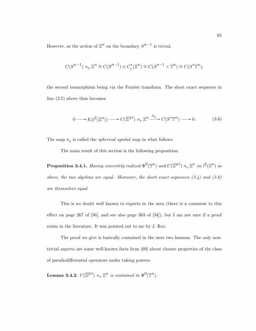
65
However, as the action of Zn on the boundary Sn−1 is trivial,
C(Sn−1) or Zn ∼= C(Sn−1)⊗ C∗r
(Zn) ∼= C(Sn−1 × Tn) ∼= C(S∗Tn),
the second isomorphism being via the Fourier transform. The short exact sequence in
line (3.5) above thus becomes
0 // K(l2(Zn)) // C(Zns) or Znσs // C(S∗Tn) // 0 . (3.6)
The map σs is called the spherical symbol map in what follows.
The main result of this section is the following proposition.
Proposition 3.4.1. Having concretely realized Ψ0(Tn) and C(Zns) or Zn on l2(Zn) as
above, the two algebras are equal. Moreover, the short exact sequences (3.4) and (3.6)
are themselves equal.
This is no doubt well known to experts in the area (there is a comment to this
effect on page 267 of [56], and see also page 303 of [34]), but I am not sure if a proof
exists in the literature. It was pointed out to me by J. Roe.
The proof we give is basically contained in the next two lemmas. The only non-
trivial aspects are some well-known facts from [69] about closure properties of the class
of pseudodifferential operators under taking powers.
Lemma 3.4.2. C(Zns) or Zn is contained in Ψ0(Tn).

66
Proof. Consider the partial differential operators
∂
∂xifor i = 1, ..., n and ∆ =
n∑i=1
∂2
∂x2i
on Rn. They are invariant for the action of Zn, so pass to differential operators (and in
particular pseudodifferential operators) of orders one and two on Tn.
Now, ∆ is positive and elliptic whence, by results of [69], the operator (1 + ∆)−12
makes sense and is pseudodifferential of order −1. This implies that the operators
∂
∂xi(1 + ∆)−
12 , i = 1, ..., n
are also pseudodifferential, this time of order zero. Under Fourier transform, they cor-
respond to the multiplication operators
ei : m = (m1, ...,mn) 7→ mi
(1 + ‖m‖22)12
acting on l2(Zn).
Further, note that∑ni=1 ei(m)2 = ‖m‖22/(1 +‖m‖22), from which one can recover
‖m‖2; hence from all the ei(m) one can recover each mi and hence m itself. This says
that the algebra generated by ei : i = 1, ..., n, separates points in Zn. Continuing,
note that ∣∣∣ei(m) =mi
(1 + ‖m‖22)12
− mi‖mi‖2
∣∣∣→ 0

67
as m → ∞; as the functions m 7→ mi/‖m‖2, i = 1, ..., n, both extend to Zns and
separate points on the boundary Sn−1, these properties are true of ei for i = 1, ..., n as
well. Hence the ei generate a C∗-subalgebra of C(Zns), and by the Stone-Weierstrass
theorem this C∗-subalgebra is actually the whole thing.
To recapitulate then, C(Zns) is generated by pseudodifferential operators of order
zero, whence is contained in Ψ0(Tn). On the other hand, C∗r
(Zn) (with respect to its
natural representation on l2(Zn)) is contained in Ψ0(Tn) as the subalgebra C(Tn). As
C∗r
(Zn) and C(Zns) together generate C(Zns) o Zn as a C∗-subalgebra of B(l2(Zn)),
the lemma follows.
The next lemma says that this inclusion is consistent with the symbol maps σΨ
and σs from (3.4) and (3.6) respectively.
Lemma 3.4.3. The restriction of σΨ from Ψ0(Tn) to C(Zns) or Zn is equal to σs.
Proof. Following the proof of the above lemma, C(Zns) or Zn is generated by the ei
and C∗r
(Zn) ∼= C(Tn), so it suffices to check that the two symbol maps agree on these
elements. In the case of C(Tn), this is simple: the image of f ∈ C(Tn) under either
symbol map is f itself pulled back to all of S∗Tn via the quotient map to Tn.
Consider again the functions ei, then. Note first that the symbol of the operators
∂
∂xi(1 + ∆)−
12 ,
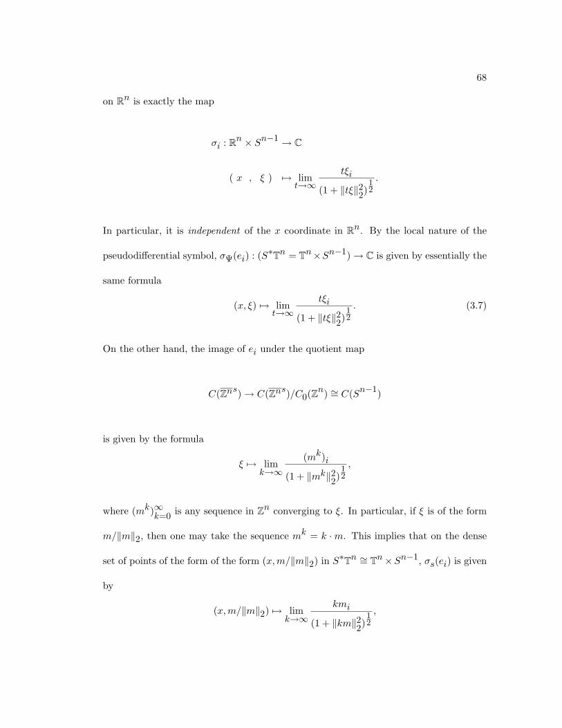
68
on Rn is exactly the map
σi : Rn × Sn−1 → C
( x , ξ ) 7→ limt→∞
tξi
(1 + ‖tξ‖22)12
.
In particular, it is independent of the x coordinate in Rn. By the local nature of the
pseudodifferential symbol, σΨ(ei) : (S∗Tn = Tn×Sn−1)→ C is given by essentially the
same formula
(x, ξ) 7→ limt→∞
tξi
(1 + ‖tξ‖22)12
. (3.7)
On the other hand, the image of ei under the quotient map
C(Zns)→ C(Zns)/C0(Zn) ∼= C(Sn−1)
is given by the formula
ξ 7→ limk→∞
(mk)i
(1 + ‖mk‖22)12
,
where (mk)∞k=0 is any sequence in Zn converging to ξ. In particular, if ξ is of the form
m/‖m‖2, then one may take the sequence mk = k ·m. This implies that on the dense
set of points of the form of the form (x,m/‖m‖2) in S∗Tn ∼= Tn×Sn−1, σs(ei) is given
by
(x,m/‖m‖2) 7→ limk→∞
kmi
(1 + ‖km‖22)12
,

69
which is the same formula as appearing in line (3.7) above. Hence σs(ei) and σΨ(ei) are
continuous functions on S∗Tn agreeing on a dense subset, so they are the same.
Proof of proposition 3.4.1. The above two lemmas say that the short exact sequences
from (3.4) and (3.6) fit into a commutative diagram
0 // K(l2(Zn)) // Ψ0(Tn)σΨ // C(S∗Tn) // 0
0 // K(l2(Zn)) // C(Zns) or Znσs //
?
OO
C(S∗Tn) // 0
;
this is only possible (by the five lemma, if you like) if the central vertical arrow is also
an equality.
3.5 Example: the visibility boundary of a CAT (0) space
In this section and the next we look at geometrically defined boundaries for certain
classes of groups. These definitions are not used for our results on Zn in chapter 5 and
section 6.1. Nonetheless, we do get certain K-theoretic results on these boundaries in
sections 4.6, 4.7 and 6.2 which mimic part of the results for Zn, as well as being of
interest in their own right.
The first of our examples comes from the action of a group on a CAT (0) space.
We assume the reader is familiar with the definition and basic properties of CAT (0)
spaces (see e.g. [9]). For ease of reference, we make the following definition.
Definition 3.5.1. A discrete group Γ is called a CAT (0) group if it acts properly
cocompactly (on the left) by isometries on a proper CAT (0) metric space.

70
In particular, the following compactification (see section II.8 of [9] for more details,
in particular definition 8.5) will be our principal object of study.
Definition 3.5.2. Let X be a proper CAT (0) metric space. Fix a basepoint x0 ∈ X.
It follows from our assumptions that for any s ≥ r ≥ 0, there exists a projection
ps,r : B(x0, s)→ B(x0, r)
defined by mapping x ∈ B(x0, s) to the unique point at distance r from x0 on the
(unique) geodesic from x to x0; see proposition II.2.4 from [9]. Moreover, if t ≥ s ≥ r,
then ps,r pt,s = pt,r, whence the balls B(x0, r) and maps ps,r form a projective system.
Define the visual compactification of X, denoted Xv, to be the inverse limit topological
space
Xv = lim←−rB(x0, r).
The visual boundary of X, denoted ∂vX, is the associated corona Xv\X.
Say that Γ is a CAT (0) group acting on X as in definition 3.5.1. As the topology
on ∂vX does not depend on the choice of basepoint, it follows that the action of Γ on X
extends to an action by homeomorphisms on Xv; see corollary II.8.8 from [9]. Moreover,
if x0 ∈ X is some choice of basepoint, we may equivariantly embed Γ into X via the
orbit map g 7→ gx0. Taking the union of this orbit with the visual boundary of X gives
a compactification ΓX of Γ, which is equivariant for the left action of Γ on itself (and
also the right action, but we will not use this).

71
If we assume moreover that Γ is exact, then there is short exact sequence
0 // K // C(ΓX ) or Γ // C(∂vX) or Γ // 0
as in proposition 3.2.1 above.
The following examples are the main motivations.
Examples 3.5.3. • Let X be a simply connected Riemannian manifold of non-positive
sectional curvature. It is a proper CAT (0) space (cf. the appendix to chapter II.1
from [9]). Fix a basepoint x0 ∈ X. Then the Cartan-Hadamard theorem states
that the exponential map exp : Tx0X → X is a diffeomorphism. Moreover, its
restriction to the unit sphere induces a homeomorphism of Sn−1 with the visual
boundary of X.
• In particular, say Γ is the fundamental group of a closed manifold M of non-positive
sectional curvature. Then the universal cover X of M is as in the above example,
and Γ is thus a CAT (0) group. The previous section can be thought of as the case
M = Tn, X = Rn, Γ = Zn.
• Let G be an almost connected Lie group whose connected component is linear and
reductive. Let K be a maximal compact subgroup. Then the symmetric space
X = G/K is a manifold of non-positive curvature, so CAT (0) by the above; see
chapter II.10 of [9] and references contained there. If Γ is a cocompact lattice in
G, then it acts properly cocompactly by isometries on G/K, so is a CAT (0) group.
It is moreover automatically exact by results of [30].

72
• Let X be an affine Bruhat-Tits building, which is a proper CAT (0) space. Then
its visual compactification is the same as its Borel-Serre compactification; [9],
appendix to chapter II.10 and references. This can be used to get results like the
above on cocompact lattices in p-adic groups.
3.6 Example: the Gromov boundary of a hyperbolic group
In this section, we discuss the case of word hyperbolic groups; see [27]. This class of
groups is automatically exact, which follows for example from [66]. We again assume the
reader is familiar with these objects (see for example [26], [27] and chapter III.H of [9]).
Nonetheless, we give some (slightly non-standard) definitions below to fix conventions.
Definition 3.6.1. Let (X, d) be a metric space and e any point in X (the notation is
meant to be reminiscent of the identity element in a discrete group). If x, y are any
elements of X, then the Gromov product of x and y with respect to e, denoted 〈x|y〉e, is
defined by
〈x|y〉e =12
(d(x, e) + d(y, e)− d(x, y));
if the basepoint e is understood, we often omit the subscript ‘e’, and write |x| for d(x, e).
Definition 3.6.2. A metric space (X, d) is called discretely geodesic if:
• the metric d is integer valued;
• for any x, y ∈ X there exists a sequence of points x0 = x, ..., xd(x,y) = y such that
d(xi, xi + 1) = 1 for all i = 0, ..., d(x, y)− 1.
A sequence of points as in the second line is called a geodesic segment in X.

73
Definition 3.6.3. Let (X, d) be a proper, discretely geodesic metric space equipped
with a basepoint e. If there exists δ ≥ 0 such that for all x, y, z ∈ X
〈x|y〉 ≥ min〈x|z〉, 〈y|z〉 − δ
then X is said to be δ-hyperbolic. X is said to be hyperbolic if it is δ-hyperbolic for some
δ ≥ 0.
Remarks 3.6.4. 1. It is not usual to demand that hyperbolic spaces are discretely
geodesic! This simplifies certain technical details in section 4.7 below, however.
Moreover, our most important class of examples consists of word hyperbolic groups
(see the next comment), and these automatically satisfy the conditions above. One
can recover a genuinely geodesic space from a discretely geodesic one by attaching
a copy of the interval [0, 1] between any points x, y ∈ X that satisfy d(x, y) = 1.
2. If X and Y are coarsely equivalent discretely geodesic metric spaces, with X hyper-
bolic then Y is also hyperbolic. In particular, one may say that a finitely generated
group Γ is (word) hyperbolic if it is a hyperbolic space with respect to a word met-
ric associated to some (finite) choice of generating set, and this does not depend
on the choice involved.
3. Let X be a proper quasi-geodesic metric space in the sense of [26] or [27]. Then it
is coarsely equivalent (in fact quasi-isometric) to one of the form in definition 3.6.3
above. In particular, there is no real loss of generality in our definition.

74
4. In fact, one can define the property of ‘being a hyperbolic space’ purely in terms of
a coarse structure on a space X: roughly, one demands that the coarse structure
be singly generated (monogenic in the language of [64], page 34) whence X is
coarsely equivalent to a discretely geodesic space (cf. proposition 2.57 of [64]);
one then translates the definitions above into the language of (monogenic) coarse
structures. We did not do this because restricting to the language of metric spaces
probably makes section 4.7 easier to read, and also as any ‘hyperbolic coarse space’
is automatically metrizable.
The definition below introduces the Gromov compactification of a hyperbolic
space. It also outlines some facts that we will need in section 4.7; see chapter 7 of
[26] for more details and proofs.
Definition 3.6.5. Let X be a hyperbolic metric space. A geodesic ray in X is an
isometric map γ : N → X. It is based at x ∈ X if γ(0) = x. If x, y are any points in X
and γ1, γ2 are geodesic rays, then the Gromov products with respect to y of x and γ1,
and of γ1 and γ2 are defined to be
〈γ1|x〉y = limn→∞〈γ1(n)|x〉y and
〈γ1|γ2〉y = limn→∞〈γ1(n)|γ2(n)〉y
if these exist, and infinity otherwise. Note that the expressions on the right-hand-side
are non-decreasing in n; in particular, the limits exist if they are bounded in n. If the
products are taken with respect to the fixed basepoint e of X, then the subscripts will
be omitted.

75
Two geodesic rays γ1, γ2 based at e are said to be equivalent if their Gromov
product (with respect to e) is infinity. The set of equivalence classes [γ] of geodesic rays
based at e is called the Gromov boundary of X and is denoted ∂gX. It can be equipped
with a metric d such that
c−1e−ε〈γ1|γ2〉 ≤ d([γ1], [γ2]) ≤ ce−ε〈γ1|γ2〉 (3.8)
for some constants c, ε > 0. This metric defines a compact topology on ∂gX.
Finally, the disjoint union of X and ∂gX can be topologised in such a way that a
sequence (xn) in X converges to [γ] ∈ ∂gX if and only if
〈xn|γ〉 → ∞ as n→∞.
The resulting space is a compactification of X called the Gromov compactification and
denoted Xg. If X is a word hyperbolic group equipped with a left-invariant word metric,
then the natural left action of Γ on itself extends to an action on the Gromov compact-
ification (this is also true of the right action, but we will not use it).
Just as in the case of the Higson corona, we use a left-invariant metric (i.e. one
that generates the left invariant coarse structure) to define the Gromov boundary of a
group; this is as the left action on the boundary defined with respect to a right-invariant
word metric is trivial.

76
Examples 3.6.6. • Say Γ is the fundamental group of a closed n-dimensional manifold
of strictly negative sectional curvature. Then Γ is word hyperbolic, and its Gromov
boundary is homeomorphic to Sn−1.
• More generally, if Γ acts properly cocompactly by isometries on a simply connected
CAT (−κ) space X for some κ > 0, then Γ is word hyperbolic and the Gromov
boundary of Γ coincides with the visual boundary of X (see also 1.4 and 1.5 from
chapter III.H in [9]).
• From a different, somewhat combinatorial viewpoint, certain small cancellation
groups are hyperbolic. See for example the appendix to [26].
• In a certain sense, word hyperbolic groups are ‘generic’ amongst all finitely pre-
sented groups; see [51] for a precise statement and proof.
• As far as I am aware, there are no known examples of hyperbolic groups that do
not act properly cocompactly on a CAT (0) space; see section 1 of [8]. On the other
hand, there are certainly CAT (0) groups that are not hyperbolic (for example, Zn).
Nonetheless, it seemed worthwhile to include hyperbolic groups separately, partly
as hyperbolicity is a well-behaved coarse invariant of a group, while the CAT (0)
property is not.
77
Chapter 4
The stable Higson corona
Recall that we are aiming for an index theorem for band-dominated operators
with slowly oscillating coefficients on Zn. An attempt at a K-theoretic proof of this fact
together with the short exact sequence in line (3.3) above naturally leads us to study the
group K1(∂hZn × Tn). Unfortunately, a theorem of Keesling (stated as theorem 4.1.4
below) implies that this group is enormous, making it very difficult to deal with for the
sort of proof we would like to give.
Playing historical revisionist, this section is motivated by the first discussion from
section 2.4, which pointed out that while K∗(C∗u
(|Zn|)) is a mess, K∗(C∗(|Zn|)) is well-
behaved. Somehow this suggests (being extremely vague) that ‘operators (or functions)
with values in the compact operators behave better’.
Continuing with the ill-formed (but often fruitful - cf. Karoubi’s conjecture in
algebraic K-theory) philosophy in the paragraph above, in this section we will pass from
the Higson corona to an analogous object ‘with values in the compacts’. This object, a
C∗-algebra called the stable Higson corona, was introduced by H. Emerson and R. Meyer
in a completely different context. Somewhat remarkably, the stable Higson corona really
does have much better K-theoretic properties than its ‘unstable’ progenitor. Thus the
comparison between the two can in fact be considered as an analogue of the above

78
situation of ‘C∗(|Zn|) versus C∗u
(|Zn|)’. There is a limit to how far this analogy can be
pushed, however: see part (3) of remarks 4.2.8 below.
The main portion of this chapter is devoted to studying the K-theory of the stable
Higson corona. Most of the K-theoretic results that we prove below follow from those of
Emerson and Meyer in [22]. Our methods are different and perhaps simpler, however, in
particular using no KK-theory. Special cases of these computations then play a central
role in the proof of theorem 5.0.1 on Zn, and we hope that certain of the more general
cases will eventually lead to index theorems on a broader class of groups.
The stable Higson corona was in fact introduced by Emerson and Meyer as part
of their work on the Novikov and Baum-Connes conjectures; see [24]. The results we
get below could be used via ideas of Emerson, Meyer and others to reprove results on
Novikov and Baum-Connes: in particular, they imply split injectivity of the Baum-
Connes assembly map for a large class of ‘non-positively curved’ groups. Although these
results are by now well-known, we hope the proofs below are of some interest; these
connections provide another motivation for many of the results in this chapter.
In order to give some background on index theoretic approaches to the Novikov
conjecture, and an overview of the K-theory groups of the Higson corona, we first look
at the ‘classical’ (i.e. early 90s!) links between these.
4.1 The ‘Higson conjecture’
The so-called ‘Higson conjecture’ (it is not entirely due to N. Higson, and turned
out to be false, hence the inverted commas) is related to index theoretic approaches to

79
the Novikov conjecture. Throughout this section, we use the general definition (A.8) of
the Higson corona. Similarly, when discussing the Roe algebra, we use definition A.9.
To motivate the Higson conjecture, assume for simplicity that Γ is a group with
classifying space BΓ realized by a closed manifold (see [41] for a more general treatment).
Then if EΓ is the universal cover of BΓ, there is a coarse assembly map
µ : K∗(EΓ)→ K∗(C∗(|Γ|)) (4.1)
(see chapter 12 of [43]). The left-hand-side is the K-homology of EΓ, which is generated
by classes of elliptic operators over this space. The assembly map takes the class of an
elliptic operator to its ‘higher index’, as discussed briefly in example 2.1.8.
Now, the image of a class [D] ∈ K∗(EΓ) under the assembly map is a homotopy
invariant. In particular, injectivity of µ implies that the class [Ds] ∈ K∗(EΓ) of the
lift of the signature operator from BΓ to EΓ is a homotopy invariant. Thus injectivity
of µ can be thought of as a Novikov-type statement, and indeed implies the Novikov
conjecture in favourable circumstances; see for example [63].
One approach to proving injectivity of µ proceeds via a study of the Higson corona.
Indeed, there is a pairing between the K-theory of the Higson corona C(∂hΓ) and that
of the Roe algebra C∗(|Γ|); in the language of section 5.3 of [43], this comes down to the
fact that
C∗(|Γ|) ⊆ D(Ch(Γ)//C0(Γ)),
with respect to any fixed ample representation of C0(Γ). See for example proposition
5.18 from [62] for a proof.

80
Consider now the short exact sequence
0 // C0(EΓ) // Ch(EΓ) // C(∂hEΓ = ∂hΓ) // 0 , (4.2)
which gives rise to a K-theory boundary map ∂ : K∗(∂hΓ)→ K∗+1(EΓ). As moreover
K∗(EΓ) pairs with the K-homology group K∗(EΓ) in the usual way, we get a diagram
of pairings
K∗(EΓ)
µ // K∗(C∗(|Γ|))
⊗ // Z ⊗oo
K∗(EΓ)
OO
K∗−1(∂hΓ)∂
oo
OO
(4.3)
(indices of K-groups are taken mod 2).
The following is proved in section 9 of [41] using the construction of the coarse
assembly map in terms of Paschke duality. It in turn builds on cohomological ideas from
chapter 5 of [62].
Theorem 4.1.1. If x ∈ K∗(EΓ) and y ∈ K∗−1(∂hΓ), then
〈x, ∂(y)〉 = 〈µ(x), y〉;
in other words, diagram 4.3 commutes.
Corollary 4.1.2. If ∂ is rationally surjective, then µ is rationally injective.
Proof. The pairing between K∗(EΓ) and K∗(EΓ) becomes nondegenerate after tensoring
with Q.

81
The statement that ∂ is surjective is (a version of what is) called the Weinberger
conjecture; see 6.33 in [62]. Versions of it have been established for certain classes of
groups: see for example [61] and [19]. Also results of section 3 of [17] relate statements
of this form to a manifold EΓ being hypereuclidean.
The Higson conjecture can then be stated as follows (see 6.35 in [62]).
Conjecture 4.1.3. The K-theory of Ch(EΓ) as in the above situation is Z (i.e. the
inclusion of the constant functions induces an isomorphism on K-theory).
The six term exact sequence in K-theory associated to the short exact sequence
in line (4.2) above shows that the Higson conjecture implies the Weinberger conjecture.
That the Higson conjecture might be true is suggested by the fact that the Higson
compactification is somewhat similar to the Stone-Cech compactification, and the latter
does have cohomological properties similar to those in the statement of the conjecture.
Unfortunately the Higson conjecture is completely false (see however [18] for an
attempt to salvage it by considering only cohomology with finite coefficients). The
following theorem is due to Keesling [47] (see also [17]).
Theorem 4.1.4. With EΓ as above, K∗(Ch(EΓ)) is always uncountable.
Amazingly, however, the ‘stable version’ of the Higson conjecture (i.e. the ana-
logue of 4.1.3 for the ‘stable Higson compactification’ of Emerson and Meyer stated in
4.2.7 below) is known to be true for many groups. Moreover, according to work of
Emerson and Meyer it has an even closer connection to the Novikov and Baum-Connes

82
conjectures than the usual Higson conjecture. It is the purpose of the next section to ex-
posit some of their work, after which the rest of this chapter establishes some properties
of the stable Higson corona, including certain cases of the ‘stable Higson conjecture’.
4.2 The ‘stable Higson conjecture’ and coarse co-assembly map
Following [24], in this section we will define the stable Higson corona, and sketch
out its relationship with the Baum-Connes and Novikov conjectures. This relationship
involves the ‘stable Higson conjecture’; the inverted commas are there as the somewhat
ad-hoc terminology was made up for the current exposition.
It may be helpful to compare the definition below with that of the (‘unstable’)
Higson corona for general coarse spaces given in A.8.
Definition 4.2.1. Let X be a coarse space and K an abstract copy of the compact
operators on a separable, infinite-dimensional Hilbert space.
If f : X → K is a bounded function and E is an entourage on X the variation of
f at scale E is defined to be
(∇Ef)(x) := sup(x,y)∈E
‖f(x)− f(y)‖.
A function f : X → K is called a Higson function if it is bounded, continuous and if for
any entourage E, (∇Ef)(x)→ 0 as x→∞ in X.
Equipped with pointwise operations and the supremum norm, the Higson func-
tions form a C∗-algebra, which it is denoted c(X) and called the stable Higson compact-
ification of X. Note that c(X) contains C0(X,K) as an ideal; the resulting quotient is

83
denoted
c(X) :=c(X)
C0(X,K)
and called the stable Higson corona of X.
Note that the stable Higson corona is in general much larger than C(∂hX,K)
(which it contains as a C∗-subalgebra); roughly speaking, the difference is that functions
in the latter algebra must have compact image in K.
The next definition gives ‘reduced’ versions of the above objects that will be very
useful for computations. The point (made precise in proposition 4.2.3 below) is that
they remove the contribution of the constant functions at the level of K-theory.
Definition 4.2.2. Fix a separable, infinite dimensional Hilbert space H, and let B(H)
be the algebra of bounded operators on H. The reduced stable Higson compactification,
denoted cr(X), is the C∗-algebra of all bounded continuous Higson functions f : X →
B(H) such that f(x)− f(y) ∈ K(H) for all x, y ∈ X.
Note that cr(X) contains C0(X,K) as an ideal; the resulting quotient is denoted
cr(X) and called the reduced stable Higson corona of X.
The following proposition records some basic properties of these objects; it com-
bines proposition 13, lemma 16 and proposition 33 from [22]. Note that proposition 13
from [22] only proves part (2) for the subcategory of C with morphisms given by equiv-
alence classes of Borel coarse maps; one can, however, extend to all of C using remark
A.6.
Proposition 4.2.3. 1. X 7→ c(X) and X 7→ cr(X) define contravariant functors on
the category CC of definition A.10.

84
2. X 7→ c(X) and X 7→ cr(X) define contravariant functors on the category C of
definition A.10.
3. If X is non-compact, the inclusions K → c(X) and K → c(X) as constant functions
induce injections on K-theory. Moreover, there are natural isomorphisms of graded
abelian groups
K∗(cr(X)) ∼=
K∗(c(X))K∗(K)
and K∗(cr(X)) ∼=
K∗(c(X))K∗(K)
for any non-compact X.
Remark 4.2.4. Note that part (3) of the above fails if X is compact. Indeed, in this case
c(X) = 0, while it is not hard to see that cr(X) is isomorphic to the Calkin algebra (on
a separable, infinite dimensional Hilbert space). In particular
Ki(cr(X)) =
0 i = 0
Z i = 1.
Now, say Γ is a discrete group and assume for simplicity that the classifying space
BΓ is realized by a finite CW complex (see [22], particularly section 4, for a more general
treatment). The construction of the reduced stable Higson corona gives rise to a short
exact sequence of C∗-algebras
0 // C0(EΓ,K) // cr(EΓ) // cr(EΓ) ∼= cr(Γ) // 0 , (4.4)
whence in turn a six-term exact sequence in K-theory.

85
Definition 4.2.5. Say Γ has finite classifying BΓ realized by a finite CW complex. The
coarse co-assembly map
µ∗ : K∗(cr(Γ))→ K∗+1(EΓ)
is the boundary map associated to the six term exact sequence above (we have used the
stability of K-theory to identify K∗+1(EΓ) ∼= K∗+1(C0(EΓ,K)).
There is also a natural pairing between the reduced stable Higson corona and
Roe algebra of a coarse space X; see the proof of theorem 36 in [22]. With respect to
this pairing, one has the analogue of theorem 4.1.1 (which justifies the name ‘coarse
co-assembly map’). A proof is sketched in theorem 36 of [22].
Theorem 4.2.6. Let Γ be a discrete group with BΓ realized by a finite CW complex
Then with respect to the pairing between K∗(EΓ) and K∗(EΓ) and the pairing between
K∗(C∗(|Γ|)) and K∗−1(cr(Γ)) one has that
〈µ(x), y〉 = 〈x, µ∗(y)〉
for all x ∈ K∗(EΓ) and y ∈ K∗−1(cr(Γ)).
We state the stable Higson conjecture as follows.
Conjecture 4.2.7. The K-theory of cr(EΓ) as in the above situation is 0.
It implies that the coarse co-assembly is an isomorphism, and thus as in corollary
4.1.2 above that the coarse assembly map in line (4.1) is rationally injective. The fol-
lowing remarks sum up some connections between the pairings discussed in this section
and the last.

86
Remarks 4.2.8. 1. There is a natural inclusion i : C(∂hX) ⊗ K → cr(X). It follows
immediately from the formula for the pairing between K∗−1(∂hX) and K∗(C∗(X))
and that for the pairing between K∗−1(cr(X)) and K∗(C∗(X)) that they commute
with i in the sense that
〈x, y〉 = 〈i∗(x), y〉
for all x ∈ K∗−1(∂hX) and y ∈ K∗(C∗(X)). In particular, then, rational nonde-
generacy of the pairing between K∗(EΓ) and K∗(EΓ) implies that
∂ : K∗−1(∂hΓ)→ K∗(EΓ)
is rationally surjective (the ‘Weinberger conjecture’ holds) if and only if the coarse
co-assembly map is rationally surjective. In particular, this suggests that from the
point of view of the Novikov conjecture the (often uncountably many) classes in
K∗(∂hEΓ) that are mapped to zero by i∗ are relatively uninteresting.
2. If both the coarse assembly and coarse co-assembly maps for a group (with, say,
finite classifying space) are isomorphisms, then the pairing between K∗−1(cr(Γ))
and K∗(C∗(|Γ|)) is rationally nondegenerate.
3. There is also a pairing between K∗−1(∂hΓ) and K∗(C∗u
(|Γ|)); given the analogies
at the start of this chapter, it seems natural to ask if there are circumstances
under which (a reduced version of) this pairing is non-degenerate. This fails badly,
however, as one can compute directly in the case Γ = Z.

87
Emerson and Meyer also get a result on the relationship between the coarse co-
assembly map and the Baum-Connes conjecture that is in a sense rather more precise
than the connections discussed above; see [24], corollary 36. The statement below gives
an important special case.
Theorem 4.2.9. Say Γ has finite classifying space BΓ, and that the coarse co-assembly
map as in definition 4.2.5 is an isomorphism (equivalently, that the stable Higson con-
jecture, K∗(cr(EΓ)) = 0, holds).
Then Γ has a dual Dirac morphism in the sense of [50]. In particular, the Baum-
Connes assembly map for Γ is split injective (with any coefficients), and the (strong)
Novikov conjecture holds for Γ.
4.3 Homological properties of the stable Higson corona
In this section we establish some ‘homological properties’ of the functors X 7→
K∗(cr(X)) and X 7→ K∗(c
r(X)) on the categories C and CC of definition A.10. The main
results are theorems 4.3.12 and 4.3.13, which say that these two functors have certain
‘coarse homotopy invariance properties’; cf. [40], section 11 of [39] and chapter 12 of
[43] for some similar results in other contexts. In the remaining sections of this chapter,
these will be used to compute K-theory groups of some examples; these computations
also imply the corresponding cases of the stable Higson conjecture 4.2.7.
Most of the ideas we use come from [44], [43] and [22], and many of the proofs are
adapted from these papers and book. Using this approach in this context was suggested
to me by J. Roe.

88
From now on, if φ : X → Y is a coarse map, then we denote by
φ] : cr(Y )→ c
r(X) and
φ∗ : K∗(cr(Y ))→ K∗(c
r(X))
its image under the functors cr(·) and K∗(cr(·)) respectively. We use the same notation
for the images of continuous coarse maps under the reduced stable Higson compactifi-
cation functor and its composition with the K-theory functor, as well as the unreduced
versions of all these functors.
We first establish a Mayer-Vietoris type sequence for the functor X 7→ K∗(cr(X)).
This requires a notion of excision appropriate to coarse spaces, which is taken from [44],
section 1, definition 1.
Definition 4.3.1. Let X be a coarse space. For any subset Y of X and entourage E,
let
N(Y,E) = x ∈ X : (x, y) ∈ E for some y ∈ Y
be the E-neighbourhood of Y in X.
Let X = A∪B be a decomposition of X into closed subspaces. It is called coarsely
excisive if for all entourages E on X, there exists an entourage F such that
N(A,E) ∩N(B,E) ⊆ N(A ∩B,F ).
The next lemma is closely related to proposition 1 from section 2 of [44].

89
Lemma 4.3.2. Let X = A ∪ B be a coarse space equipped with a decomposition into
closed subsets. Let iA : A → X, iB : B → X, jA : A ∩ B → A, jB : A ∩ B → B be the
associated inclusion maps.
Then if X = A ∪B is coarsely excisive there is a pullback diagram
cr(X)i]A //
i]B
cr(A)
j]A
cr(B)j]B // cr(A ∩B)
. (4.5)
Proof. Note first that pullbacks always exist in the category of C∗-algebras and ∗-
homomorphisms: the pullback P over the diagram
P //
cr(A)
j]A
cr(B)j]B // cr(A ∩B)
can be concretely constructed as
P = (a, b) ∈ cr(A)⊕ c
r(B) : j]A
(a) = j]B
(b),
equipped with the obvious projection maps to cr(A) and cr(B).
If Y is a coarse space, denote the image of f ∈ cr(Y ) under the quotient map to
cr(Y ) by [f ]. To show the existence of the diagram (4.5) above it suffices to prove that

90
the map cr(X)→ P defined by
[f ] 7→ ([f |A], [f |B ]) (4.6)
is an isomorphism of C∗-algebras. It is not hard to check that it is a well-defined,
injective ∗-homomorphism. Surjectivity is shown below.
Say then that ([gA], [gB ]) is an element of P . It follows from the definition of P
that there exists h ∈ C0(A ∩ B,K) such that gA − gB = h on A ∩ B. Surjectivity of
the restriction map C0(B,K) → C0(A ∩ B,K) implies that h extends to an element of
C0(B,K), which will also be denoted h. Define a function f : X → K by
f(x) =
gA(x) x ∈ A
gB(x) + h(x) x ∈ B.
This is well-defined as gA(x) = gB(x)+h(x) on A∩B. If f is in cr(X), then [f ] ∈ cr(X)
maps to ([gA], [gB ]) under the ∗-homomorphism in line (4.6) above. Now, f is continuous
and bounded as gA and gB + h are, and as they agree on the closed subset of X where
both are defined. Moreover, assuming A and B are non-empty (indeed, if one is empty
the lemma is trivial), the coarse excisiveness condition forces A ∩ B to be non-empty,
whence f(x) − f(y) is compact for all x, y ∈ X. It thus suffices to show that f is of
vanishing variation.

91
To this end, let E be an entourage and ε > 0. Then there exists an entourage F
containing E such that
N(A,E) ∩N(B,E) ⊆ N(A ∩B,F ).
Moreover, by vanishing variation of gA on A and gB + h on B, there exist compact
subsets KA ⊆ A, KB ⊆ B such that for all a ∈ A\KA (resp. b ∈ B\KB)
|(∇F gA)(a)| < ε (resp. |(∇F (gB + h))(b)| < ε).
Adopting the convention that if one of (∇F f)(x), (∇F g)(x) doesn’t make sense then we
just set it zero, it follows that for all x ∈ X\(KA ∪KB),
|(∇Ef)(x)| ≤ max|(∇F gA)(x)|, |(∇F (gB + h))(x)| < ε.
This shows that f has vanishing variation, completing the proof.
One also has the corresponding lemma for the compactification functor.
Lemma 4.3.3. Let X = A ∪B be a proper metric space equipped with a decomposition
into closed subsets. Let iA : A→ X, iB : B → X, jA : A ∩B → A, jB : A ∩B → B be
the associated inclusion maps.

92
Then if X = A ∪B is coarsely excisive there is a pullback diagram
cr(X)i]A //
i]B
cr(A)
j]A
cr(B)j]B // cr(A ∩B)
. (4.7)
Proof. Essentially the same as (and slightly easier than) that of lemma 4.3.2
The second ingredient needed to establish a Mayer-Vietoris sequence is surjectivity
of the restriction maps j]A and j]B . Unfortunately I do not know a proof of this in general,
but one does have the following lemma for the case of metric spaces.
Lemma 4.3.4. Let X be a proper metric space and A ⊆ X a closed subspace. Then the
restriction ∗-homomorphism
cr(X)→ c
r(A)
is surjective.
The proof of lemma 4.3.4 is somewhat technical, and we do not need it to prove
our main homotopy invariance results; it is thus postponed until the end of the section.
Note that the analogous result for the ‘unstable’ Higson corona follows in full generality
by the same argument as used to prove theorem 1.4 from [19].
The existence of Mayer-Vietoris sequences as set out below follows from the two
preceding lemmas.
Proposition 4.3.5. Let X = A∪B be a coarsely excisive decomposition and iA, iB , jA, jB
be as in the lemma 4.3.2. Assume that j]A and j]B are surjective (so in particular this
holds if X is metrizable by lemma 4.3.4).

93
Then there exists a Mayer-Vietoris sequence
// Ki(cr(X))
i∗A⊕i∗B// Ki(c
r(A))⊕Ki(cr(B))
j∗A−j∗B// Ki(c
r(A ∩B)) // .
It is moreover natural for morphisms of excisive decompositions in the category C in the
obvious sense.
Proposition 4.3.6. Let X = A∪B be a coarsely excisive decomposition and iA, iB , jA, jB
be as in the lemma 4.3.3. Assume that j]A and j]B are surjective (so in particular this
holds if X is metrizable by lemma 4.3.4).
Then there exists a Mayer-Vietoris sequence
// Ki(cr(X))
i∗A⊕i∗B// Ki(c
r(A))⊕Ki(cr(B))
j∗A−j∗B// Ki(c
r(A ∩B)) // .
It is moreover natural for morphisms of excisive decompositions in the category CC in
the obvious sense.
Emerson and Meyer point out that something like this exists ([22] remark 35),
but do not develop it any further.
Proof. This is a special case of the general notion of Mayer-Vietoris sequence associated
to a pullback diagram of C∗-algebras (see for example [7], 21.3.2) such that the right-
hand and bottom maps are surjective. The naturalness follows from naturalness for this
general Mayer-Vietoris sequence with respect to morphisms of pullback diagrams.

94
These results are of interest in of themselves, but we will only use a very special
case of them as a crutch to theorems 4.3.12 and 4.3.13.
The second ingredient used in the proofs of these results is a vanishing theorem
for coarsely flasque spaces (cf. [43], lemma 6.4.2). These are defined below.
Definition 4.3.7. Let X be a coarse space. It is coarsely flasque if there exists a
continuous coarse map φ : X → X such that:
• φ is close to the identity in the sense of definition A.4;
• for all compact subsets K ⊆ X there exists NK ∈ N such that for all n ≥ NK and
x ∈ X, φn(x) 6∈ K;
• for all entourages E there exists an entourage FE such that for all (x, y) ∈ E and
n ∈ N, (φn(x), φn(y)) ∈ FE .
X is called flasque (with apologies for the ad-hoc use of this terminology) if it is
both coarsely flasque and properly homotopic to the empty set.
The prototypes of flasque spaces are those of the form X = Y × [0,∞) where Y
is a coarse space, X is equipped with the product coarse structure (see definition A.7)
and φ is defined by φ : (y, t) 7→ (y, t + 1). Y × N is an example of a coarsely flasque
space that is not flasque (unless Y is empty). The examples we will actually use (in the
proofs of theorems 4.3.12 and 4.3.13) are only slightly more complicated than these.
The following now gives a vanishing result for the K-theory of the corona functor;
it has as a corollary a similar vanishing theorem for the compactification functor. The
proof is essentially the same as that of theorem 30 from [22].
95
Proposition 4.3.8. Let X be a coarsely flasque space. Then
K∗(cr(X)) = 0.
Proof. There is a separable infinite-dimensional Hilbert space implicit in the definition of
cr(X); denote it by H and decompose it as an infinite direct sum of infinite-dimensional
subspaces
H = ⊕n∈NHn.
For each n let Vn : H → Hn be a unitary isomorphism and define maps
νn : cr(X)→ c
r(X)
f 7→ VnfV∗n.
Let now φ : X → X be a map as in the definition of coarsely flasque space and
(provisionally) define a map ν : cr(X)→ cr(X) via
f 7→ ⊕n∈N νn(f φn).
To show that this is well-defined, it suffices to check that:
• νf is continuous. Fix ε > 0 and x ∈ X. Let E be an entourage such that
U0 = y ∈ X : (x, y) ∈ E

96
is a compact neighbourhood of x. Let FE be as given in the definition of φ, so in
particular (φn(x), φn(y)) ∈ FE for all y ∈ U0 and n ∈ N . As f is of vanishing
variation there exists a compact subset K of X such that (∇FEf)(y) < ε for
all y 6∈ K. Let NK be such that φn(y) 6∈ K for all y ∈ X and n > NK . Using
continuity of f and φ there exists a neighbourhood U of x such that for all n ≤ NK
and all y ∈ U , ‖f φn(x)− f φn(y)‖ < ε.
Now,
(νf)(x)− (νf)(y) = ⊕n∈NVn(f(φn(x))− f(φn(y)))V ∗n, (4.8)
whence for all y ∈ U , the norm of (νf)(x)− (νf)(y) is bounded by
supn∈N‖f(φn(x))− f(φn(y)‖ ≤ ε
by the assumptions above. This proves continuity of νf .
• (νf)(x) − (νf)(y) ∈ K for all x, y ∈ X. By assumption on φ, for any x, y ∈ X,
there exists an entourage F on X such that (φn(x), φn(y)) ∈ F for all n, whence
‖f(φn(x))− f(φn(y))‖ converges to zero as n→∞ (as f is of vanishing variation,
and φn(x), φn(y) eventually leave all compact subsets of X). Hence the expression
on the right hand side of line (4.8) is a direct sum of compact operators on disjoint
spaces with norms converging to zero. It is thus compact.
• νf is of vanishing variation. Let E be an entourage and ε > 0. Let FE be as in the
definition of φ. We may assume that FE contains E. Then by vanishing variation
of f there exists compact K ⊆ X such that for all x ∈ X\K, |(∇FEf)(x)| < ε.

97
Moreover, by assumption on φ, there exists NK such that for all n ≥ NK and all
x ∈ X, φn(x) 6∈ K. As φ is assumed close to the identity, there exists an entourage
F containing the diagonal such that for all x ∈ X, (x, φ(x)) ∈ F ; define
Fn = F F ... F︸ ︷︷ ︸n
(cf. definition A.1) and
K′ = N(K,
NK⋃n=1
Fn),
which is compact by compatibility of the coarse structure and topology on X. For
all x 6∈ K′ and any n ∈ N :
– if n < NK then (x, φn(x)) ∈ ∪NKn=1Fn and φn(x) 6∈ K;
– if n ≥ NK then φn(x) 6∈ K by assumption on NK .
Either way, for any (x, y) ∈ E ⊆ FE and any n ∈ N, the term Vn(f(φn(x)) −
f(φn(y))V ∗n
in line (4.8) above has norm at most ε. The norm of νf(x)− νf(y) is
just the supremum of the norms of the terms in (4.8), however, so it too has norm
at most ε. Hence νf is of vanishing variation.
Thus ν is indeed well-defined. It also preserves C0(X,K), so passes to a map
ν : cr(X)→ cr(X).

98
Now, let f, g be elements of (the unitization of) cr(X) defining some class [f ]−[g] ∈
K∗(cr(X)) (any element in this group can be written in this form). Then
ν∗([f ]− [g]) = (ν0)∗([f ]− [g])⊕([ ∑
n≥1νn(f φn−1)
]−[ ∑n≥1
νn(g φn−1)]), (4.9)
where we have used that φ induces the identity map on cr(X). Note, moreover, that
the map ν0 defines the identity on K-theory (this is always true of the map induced on
K-theory by conjugation by an isometry in the multiplier algebra), while the element
[∑n≥1 νn(f φn−1)] is conjugate via another isometry to νf , and similarly with g in
place of f . Hence (4.9) above becomes
ν∗([f ]− [g]) = [f ]− [g] + ν∗([f ]− [g]),
so [f ]− [g] = 0 and finally K∗(cr(X)) = 0.
Proposition 4.3.9. Let X be a flasque space. Then
K∗(cr(X)) = 0.
Proof. By the previous proposition, K∗(cr(X)) = 0, while K∗(C0(X,K)) = 0 by the
fact that X is properly homotopic to the empty set. The result now follows from the
K-theory long exact sequence associated to the short exact sequence
0 // C0(X,K) // cr(X) // cr(X) // 0 .

99
Example 4.3.10. We now have enough information to compute K-theory groups in the
case of Rn. Indeed, using example 4.2.4, proposition 4.3.5, lemma 4.3.4, proposition
4.3.8 and induction on n one can show that
Ki(cr(Rn)) =
Z i = n+ 1 mod 2
0 i = n mod 2.
The main aim of this section is to combine the results of propositions 4.3.5 and
4.3.8 (resp. 4.3.6 and 4.3.9) to get homotopy invariance results. The notion of homotopy
we use is as follows. It is almost the same as that in [39] section 11.
Definition 4.3.11. Let φ0, φ1 : X → Y be morphisms in the category CC. They are
said to be elementary continuous coarse homotopy equivalent if there exists a continuous
map H : X × R+ → Y and a continuous coarse map X → R+ denoted x 7→ tx such
that:
• H(x, 0) = φ0(x) for all x ∈ X;
• for all t ≥ tx, H(x, t) = φ1(x);
• if Z := (x, t) ∈ X × R+ : t ≤ tx is equipped with the restriction of the product
coarse structure on X × R+, then H restricted to Z is coarse.
Such an H is called an elementary continuous coarse homotopy equivalence between φ0
and φ1.
Continuous coarse homotopy equivalence is then the equivalence relation on mor-
phisms in CC generated by elementary coarse equivalence.

100
To get the definition of coarse homotopy equivalence, replace R+ by N, CC by C
and remove the word ‘continuous’.
Note that coarse homotopy equivalence is a strictly finer equivalence relation
than continuous coarse homotopy equivalence: if H is an elementary continuous coarse
homotopy equivalence, then its restriction to X × N is an elementary coarse homotopy
equivalence.
The following proof is taken from [43], proposition 12.4.12.
Theorem 4.3.12. Let φ0, φ1 : X → Y be morphisms in the category CC that are con-
tinuously coarsely homotopic. Then the induced maps
φ∗0, φ∗1 : K∗(c
r(Y ))→ K∗(cr(X))
are the same.
Proof. It suffices to show the result when φ0, φ1 are elementary continuous coarse ho-
motopy equivalent. Let H : X×R+ → Y be an elementary continuous coarse homotopy
equivalence, which we extend to all of X × R by defining H(x, t) = H(x, 0) for t < 0.
Give X × R the product coarse structure (definition A.7) and define
Z := (x, t) ∈ X × R : x ∈ X, 0 ≤ t ≤ tx.
Further, define inclusion maps i0, i1 : X → Z by
i0(x) = (x, 0) and i1(x) = (x, tx);

101
i0 is clearly coarse, while i1 is coarse by definition of an elementary continuous coarse
homotopy equivalence. Note also that H is continuous and coarse when restricted to Z,
and that
H ij = φj for j = 0, 1. (4.10)
Let moreover π : Z → X be the coordinate projection onto the X variable. We first
claim that the maps
i∗0, i∗1 : K∗(c
r(X)→ K∗(cr(Z))
are in fact equal.
Indeed, extend π as a coordinate projection to all of X × R. Let A = (x, t) ∈
X × R : t ≤ 0, A′ = (x, t) ∈ X × R : t ≤ tx and B = (x, t) ∈ X × R : t ≥ 0. Then
both of the decompositions X = A∪B and X = A′ ∪B are coarsely excisive. Moreover,
it is not too hard to see that the restriction ∗-homomorphisms
cr(X × R)→ c
r(Y )
are surjective for Y = A,A′, B; for example, in the case of B, any f ∈ c(B) extends to
a function f ∈ cr(X × R) via the formula
f(x, t) =
f(x, t) t < 0
f(x,−t) t ≥ 0,
and the other cases are similar. Note also that the identity map on X × R is a map
of such decompositions in the category CC, whence from proposition 4.3.6 there is a

102
commutative diagram of Mayer-Vietoris sequences
// Ki(cr(X × R)) // Ki(c
r(A))⊕Ki(cr(B)) // Ki(c
r(A ∩B)) //
// Ki(cr(X × R)) //
OO
Ki(cr(A′))⊕Ki(c
r(B)) //
OO
Ki(cr(A′ ∩B)) //
OO.
The first vertical arrow is an isomorphism as induced by the identity map. The second
is also an isomorphism as both its domain and codomain vanish by flasqueness of A, A′
and B, and proposition 4.3.9. Hence the third vertical map is an isomorphism by the
five lemma. It is, however, exactly the map i∗0 : K∗(cr(Z))→ K∗(c
r(X)).
Now, π∗ is a one-sided inverse to i∗0; as i∗0 is an isomorphism, π∗ is an isomorphic
two-sided inverse. As π∗ is a one-sided inverse to i∗1 and an isomorphism, i∗1 is an
isomorphism, and two-sided inverse to π∗. Hence in particular, i∗0 and i∗1 are both equal
to (π∗)−1, so equal.
To finish the proof, then, looking back at line (4.10) above, we see that
i∗jH∗ = φ∗
j: K∗(c
r(Y ))→ K∗(cr(X))
for j = 0, 1. As i∗0 = i∗1, however, φ∗0 = φ∗1 as claimed.
Theorem 4.3.13. Let φ0, φ2 : X → Y be morphisms in the category C that are coarsely
homotopic. Then the induced maps
φ∗0, φ∗1 : K∗(c
r(Y ))→ K∗(cr(X))

103
are the same.
Proof. Same as that of the previous proposition, but replace R+ by N, R by Z, cr(X)
by cr(X) and remove the word ‘continuous’.
Remark 4.3.14. It will be useful in section 4.7 that one has the same homotopy invariance
results for the ‘unreduced’ functors X 7→ K∗(c(X)) and X 7→ K∗(c(X)). The proofs are
essentially the same; we did not state them explicitly above out of fear of too much
tedious repetition.
The final result in this section is another vanishing result, closely related to propo-
sition 57 from [22]. It is our main computational tool. It does not seem to be possible
to make sense of it without at least a uniform structure on X. We thus restrict to the
case of metric spaces for the remainder of this section, including the postponed proof of
lemma 4.3.4.
Definition 4.3.15. Let X be a proper metric space. A continuous coarse map s : X →
X is called a scaling if for all x, y ∈ X, d(s(x), s(y)) ≤ d(x, y)/2.
The proof of the following vanishing result is essentially the same as that of
theorem 12.4.11 from [43]; it is another Eilenberg swindle.
Proposition 4.3.16. Say s : X → X is a scaling. Then the map
s∗ : K∗(cr(X))→ K∗(c
r(X))
is zero.

104
Proof. Choose a decomposition H = ⊕n∈NHn, and corresponding unitaries Vn and
conjugating maps νn as in proposition 4.3.8. (Provisionally) define a map from cr(X)
to itself via the formula
ν : f 7→ ⊕n∈N νn(f sn);
if this is well-defined, essentially the same Eilenberg swindle as in proposition 4.3.8
completes the proof (note that this map does not preserve C0(X,K), so does not pass
to the corona cr(X)).
Just as in the earlier proposition, we must check three conditions. The only real
observation is that because f is of vanishing variation, it is uniformly continuous, whence
the (global) modulus of continuity of f sn gets arbitrarily small as n tends to infinity.
The details are below.
• νf is continuous. As s is a contraction and f is uniformly continuous, all the maps
f sn are equicontinuous, whence νf itself is continuous.
• (νf)(x)−(νf)(y) is compact for all x, y ∈ X. Note that as f is uniformly continuous
and for any x, y ∈ X d(sn(x), sn(y))→ 0 as n→∞, it follows that (νn(fsn))(x)−
(νn(f sn))(y) tends to zero as n → ∞. Hence (νf)(x) − (νf)(y) consists of an
infinite direct sum of compact operators whose norms tend to zero at infinity. It
is thus compact.
• νf is of vanishing variation. Let R, ε > 0. As f is uniformly continuous, there
exists δ > 0 such that d(x, y) < δ implies ‖f(x) − f(y)‖ < ε. Let N be such that
for all n ≥ N and all x, y ∈ X such that d(x, y) ≤ R, d(sn(x), sn(y)) < δ. Further,
as f is of vanishing variation, there exists compact K ⊆ X such that if x, y /∈ K

105
and d(x, y) ≤ R, then ‖f(x) − f(y)‖ < ε. Let K′ = ∪n<N (sn)−1(K) (which is
compact as s is proper). It follows that for all x, y /∈ K′ such that d(x, y) ≤ R,
‖(νf)(x)− (νf)(y)‖ < ε. Hence νf is of vanishing variation.
As promised, we finish this section with the proof of lemma 4.3.4.
Proof. Let f ∈ cr(A) and ε > 0. As ∗-homomorphisms have closed image, it suffices to
prove that there exists f ∈ cr(X) such that ‖f(a)− f(a)‖B(H) < ε for all a ∈ A.
Let first
v : A→ R ∪ ∞
be any non-decreasing (with respect to distance from some fixed base-point a0 ∈ A)
function tending to infinity at infinity in A and such that
• v(a) ≤ supR > 0 : (∇Rf)(a) < ε for all a ∈ A;
• (∇v(a)f)(a)→ 0 as a→∞.
Such a v exists by vanishing variation of f . Further, for each a ∈ A, let
Ua = BX (a,√v(a)),
the open ball in X about a of radius√v(a). Let ρ : R+ → R+ be any non-decreasing,
subadditive function such that ρ(0) = 0, ρ(t) > 0 for all t > 0, ρ(t)→∞ as t→∞ and
so that for all x ∈ X
d(x,A) ≤ ρ(d(x, a0)) implies x ∈ ∪a∈AUa.

106
One may then define
F = x ∈ X : d(x,A) ≤ ρ(d(x, a0)),
a closed subset of X containing A and covered by Uaa∈A. Let φii∈I be a locally
finite continuous partition of unity on F subordinate to Ua. For each i ∈ I, let ai ∈ A
be such that φi is supported in Uai. Using Tietze’s extension theorem, extend each φi
to a [0, 1]-valued function defined on all of X and supported in Uai. Finally, define a
function
ψ : X → R+
x 7→ maxρ(d(x, a0))− d(x,A)
ρ(d(x, a0)), 0
(which is supported in F , and equal to one on A) and define
f : X → C
x 7→ ψ(x)∑i∈I
φi(x)f(ai).
The choice of the cover Ua guarantees that ‖f(a)− f(a)‖ < ε for all a ∈ A, and
moreover f is bounded, continuous, supported in F and satisfies f(x)− f(y) ∈ K for all
x, y ∈ X. To finish the proof of the lemma it thus suffices to prove that f is of vanishing
variation.

107
To this end, say x, y ∈ X satisfy d(x, y) ≤ R for some R > 0. Then
‖f(x)−f(y)‖
≤ |ψ(x)|∥∥∥∑i∈I
(φi(x)− φi(y))f(ai)∥∥∥+ |(ψ(x)− ψ(y))|
∥∥∥∑i∈I
φi(y)f(ai)∥∥∥
≤ |ψ(x)|∥∥∥∑i∈I
(φi(x)− φi(y))f(ai)∥∥∥+ |ψ(x)− ψ(y)|‖f‖cr(A)
Assume without loss of generality that ψ(x), ψ(y) do not both vanish.
Case (1): Exactly one of ψ(x), ψ(y) is zero.
Without loss of generality, assume that ψ(x) vanishes. Then the above becomes
‖f(x)− f(y)‖ ≤ |ψ(y)|‖f‖ =(ρ(d(y, a0))− d(y,A)
ρ(d(y, a0))
)‖f‖
≤(ρ(d(x, a0)) + ρ(R)− d(x,A) +R
ρ(d(y, a0))
)‖f‖
using subadditivity of ρ. By assumption that ψ(x) = 0, this in turn is bounded by
( ρ(R) +R
ρ(d(y, a0))
)‖f‖,
which gets arbitrarily small as long as y gets far from a0.
Case (2): Both of ψ(x), ψ(y) are non-zero.
Using a similar argument to that in case (1), |ψ(x)−ψ(y)| can be made arbitrarily small
by assuming that x, y are suitably far from a0. It thus remains to show that the term
|ψ(x)|∥∥∥∑i∈I
(φi(x)− φi(y))f(ai)∥∥∥ ≤ ∥∥∥∑
i∈I(φi(x)− φi(y))f(ai)
∥∥∥

108
can be made arbitrarily small by assuming x and y are suitably far from a0. Now, by
assumption that ψ(x) 6= 0 6= ψ(y), it follows that x, y ∈ F , whence there exist ax, ay ∈ A
such that d(ax, x) ≤√v(ax) and d(ay, y) ≤
√v(ay). Moreover, as v(a)→∞ as a→∞
in A, if x, y ∈ X are suitably far from a0, then if i ∈ I satisfies either φi(x) 6= 0 or
φi(y) 6= 0, then d(ai, ax) ≤ v(ax). Finally, then, by assumption that (∇v(a)f)(a) → 0
as a→∞,
∥∥∥∑i∈I
(φi(x)− φi(y))f(ai)∥∥∥ ≤ ∥∥∥f(ax)−
∑i∈I
φi(x)f(ai)∥∥∥+
∥∥∥f(ax)−∑i∈I
φi(y)f(ai)∥∥∥
can be made arbitrarily small for ax suitably far from a0 (which in turn can be forced
by stipulating that x, y are suitably far from a0). This completes the proof.
4.4 Geometric boundaries
The aim of the next four sections is to compute K∗(c(X)) (and also prove the sta-
ble Higson conjecture 4.2.7) in certain cases. These results are mainly already contained
in, or follow easily from, [22], but the proofs are somewhat different.
We put particular emphasis on the fact that the inclusion of the (stabilised) con-
tinuous functions on a geometric boundary ∂X of X into c(X) induces an isomorphism
on K-theory. In some cases, this allows for a description of K∗(c(X)) in terms of specific
geometrically defined generators, although we do not pursue this. In the main cases
of interest, the geometric boundaries we use are the visual and Gromov boundaries in-
troduced in sections 3.5 and 3.6; their existence thus rely on some sort of ‘non-positive

109
curvature’ assumption on the original space X.
This preliminary section introduces the general setup for the specific results that
follow. The next definition is very close to definition 10.6.7 from [62] and also to definition
5.13 in [43].
Definition 4.4.1. Let X be a coarse space and X a compactification of X. X is called
a geometric compactification if the canonical inclusion C0(X) → Ch(X) extends to an
inclusion
C(X)→ Ch(X).
Equivalently, X is geometric if any continuous function on it is of vanishing vari-
ation when restricted to X. The Higson compactification is itself geometric, and is in a
reasonable sense the largest geometric compactification. Further examples are the visual
and Gromov compactifications for appropriate X; see lemmas 4.6.2 and 4.7.1.
The following simple lemma extends this inclusion property to the Higson corona
and stable Higson corona.
Lemma 4.4.2. Say X is a geometric compactification of X and ∂X = X\X the asso-
ciated corona. Then there are natural inclusions
C(∂X)→ C(∂hX)
C(∂X)⊗K → c(X)

110
Proof. The first inclusion is immediate from the definition. For the second, note that if
X is geometric, there are natural inclusions
C(X,K) → C(Xh,K) → c(X),
where the second inclusion is given by restriction to X (note that it is never an equality
if X is non-compact). Moreover, these inclusions preserve the ideal C0(X,K) in each
case, and there is thus a natural inclusion of quotients
C(∂X)⊗K ∼=C(X,K)C0(X,K)
→ c(X)C0(X,K)
∼= c(X).
4.5 Open cones
Our first application is to open cones. From a certain point of view, the cases
covered in sections 4.6 and 4.7 below are accessible to our methods because non-positive
curvature conditions can be used to show that they have a ‘cone-like’ structure over
a geometric boundary. The class of open cones over compact metric spaces is thus a
(simple) prototype for what follows, as well as containing some interesting examples in
its own right.
The definition of an open cone we use is as follows.
Definition 4.5.1. Let Y be a compact metric space of diameter at most 2. The open
cone over Y , denoted OY , is
OY := (Y × R+)/(Y × 0)

111
as a topological space. If s ∈ R+ and y ∈ Y , a general point in OY will be denoted sy.
The open cone is equipped with the ‘l1-type’ metric
dOY (sx, ty) := |t− s|+ mins, td(x, y). (4.11)
Some remarks are perhaps in order here.
Remarks 4.5.2. 1. The expression dOY above really is a metric. The condition that
the diameter of Y is at most two is important here.
2. As Y is compact, OY is a proper metric space.
3. It is perhaps more usual to assume that Y is a subset of the unit sphere in some
Hilbert space H, and define the open cone over Y to be
ty ∈ H : t ∈ R+, y ∈ Y
equipped with the restriction of the metric from H. If Y does start out as a subset
of a sphere in this way, then it is not hard to check that the two definitions of ‘open
cone’ define coarsely equivalent metric spaces.
4. As an example that we will use later, say Y is Sn−1, equipped with either its
intrinsic metric or the restricted metric from Rn. Then OY is coarsely equivalent
to Rn equipped with the Euclidean metric.
5. There is a natural compactification of OY defined by attaching a copy of Y at
infinity. Indeed, identify OY with the space ([0, 1) × Y )/(Y × 0) ⊂ ([0, 1] ×

112
Y )/(Y × 0) via some homeomorphism ρ : [0, 1) → [0,∞) (which must fix zero
and be increasing). Then the compactification can be defined to be [0, 1]×Y/Y×0
(it does not depend on the choice of ρ).
Denote by OY the compactification of OY appearing in the final point above.
The following simple lemma says that this is a geometric compactification in the sense
of definition 4.4.1.
Lemma 4.5.3. OY is a geometric compactification of OY .
Proof. Let R, ε > 0. Let ρ : [0,∞) → [0, 1) be some homeomorphism (fixing zero) as in
the remark, and note that OY can be metrized using the expression in line (4.11) above.
Let f be a continuous function of OY , so in particular f is uniformly continuous. Let
δ > 0 be such that if dOY (x1, x2) ≤ δ then |f(x)− f(y)| < ε.
Now, for any R > 0 there exists S > 0 so that if t1, t2 > S then |ρ(t1)− ρ(t2)| <
δ/2 and R/S ≤ δ/2. It follows that if t1y1, t2y2 ∈ OY satisfy dOY (t1y1, t2y2) ≤ R and
t1, t2 > S, then
dOY (ρ(t1)y1, ρ(t2)y2) = |ρ(t1)− ρ(t1)|+ minρ(t1)ρ(t2)dY (y1, y2)
≤ |ρ(t1)− ρ(t2)|+ dY (y1, y2)
< R/S + δ/2 < δ.
Hence |f(t1y1)− f(t2y2)| < ε.

113
From lemma 4.4.2 then, there is a natural inclusion
iY : C(Y )⊗K → c(OY ). (4.12)
The main result of this section, and the prototype for the main results of the next
two sections, is the following.
Proposition 4.5.4. iY as in line (4.12) above induces an isomorphism on K-theory.
Proof. Note that the map
s : OY → OY
ty 7→ (t/2)y
is both a scaling and continuously coarsely homotopic to the identity; proposition 4.3.16
and theorem 4.3.12 thus show that the map
s∗ : K∗(cr(OY ))→ K∗(c
r(OY ))
is both zero and an isomorphism. Hence the group appearing in the above line is zero.
Note that this statement could be thought of as saying thatOY satisfies the stable Higson
conjecture 4.2.7 (strictly, however, that conjecture involves a group, so this doesn’t make
literal sense).

114
Consider now the commutative diagram of short exact sequences
0 // C0(OY,K) // C(OY ,K) _
// C(Y,K) _
iY
// 0
0 // C0(OY,K) // c(OY ) // c(OY ) // 0
.
OY is compact and contractible, whence its K-theory is generated by the constant
map to any rank one projection in K; by the paragraph at the start of the proof and
proposition 4.2.3, the same is true of c(OY ). Hence the central vertical map induces an
isomorphism on K-theory and so by the long exact sequence in K-theory and the five
lemma, iY does too.
4.6 CAT (0) spaces
This section looks at CAT (0) spaces. The visual compactification of such a space,
as introduced in section 3.5, will be our main tool. The following lemma is well-known,
but we couldn’t find a proof in the literature so give one one below for completeness.
Lemma 4.6.1. Let X be as in definition 3.5.2. Then the visual compactification Xv of
X is contractible.
Proof. From the definition of the visual compactification, a point in Xv is the same thing
as a ‘[0,∞) indexed set’ (yr)r∈[0,∞) such that for all t ≥ s ≥ r, pt,r(ys) = yr. For each
t ∈ [0, 1) and any (yr) ∈ Xv, define
ytr
=
yr 0 ≤ r < t
1−t
y t1−t
t1−t ≤ r <∞
.

115
If t = 1, set (ytr) = (yr). The formula
H : Xv × [0, 1]→ Xv
((yr), t) 7→ (ytr)
defines a contracting homotopy of Xv.
Lemma 4.6.2. Let X be as in definition 3.5.2. Then the visual compactification of X
is geometric.
Proof. See definition 3.5.2 for the notation used below. From the Gelfand-Naimark
equivalence of categories and general nonsense,
C(Xv) = lim−→C(B(x0, r)),
where the connecting maps in the inductive system are those functorially induced by
ps,r. It follows that C(Xv) has a dense subalgebra consisting of functions f such that
there exists r0 > 0 such that for all x 6∈ B(x0, r0), f(x) = f(pd(x0,x),r0(x)). In other
words, outside of B(x0, r0), f is ‘constant on radial lines’. It suffices to prove that any
such f is of vanishing variation when restricted to X.
To this end, let R, ε > 0, and note that f is uniformly continuous on B(x0, r0)
(with r0 as above), so there exists δ > 0 such that d(x, y) < δ implies |f(x)− f(y)| < ε.
Moreover, it follows from the CAT (0) inequality that there exists s > 0 such that
for all x, y 6∈ B(x0, s) with d(x, y) ≤ R and all t ≥ d(x, x0), d(y, x0), r one has that

116
d(pt,r0(x), pt,r0(y)) < δ. Hence
|f(x)− f(y)| = |f(pt,r0(x))− f(pt,r0(y))| < ε,
whence f is of vanishing variation as required.
Again, then, there is a canonical inclusion
iv : C(∂vX)⊗K → c(X).
The next proposition is the main result of this section.
Proposition 4.6.3. The inclusion iv defined above induces an isomorphism on K-
theory. Moreover the stable Higson conjecture 4.2.7 holds for a group that acts freely
properly cocompactly by isometries on a CAT (0) space.
Proof. Fix any basepoint x0 ∈ X. Then any x ∈ X is connected to x0 via a unique
geodesic, say γx : [0, d(x0, x)]→ X. Assume that each γx is oriented so that γx(0) = x0,
γx(d(x0, x)) = x, and define a map
s : X → X
x 7→ γx(d(x0, x)/2),
which is a continuous coarse map. It follows immediately from the CAT(0) inequality
that s is a scaling. Moreover, s is continuously coarsely homotopic to the identity via

117
the map
H : X × R+ → X
(x, t) 7→
γx(d(x0, x)− t) 0 ≤ t < d(x0, x)/2
γx(d(x0, x)/2) t ≥ d(x0, x)/2.
Just as in proposition 4.5.4, it follows that K∗(cr(X)) = 0. Note in particular that if Γ
acts freely, properly, cocompactly and by isometries on X then X can itself be taken as
an EΓ. Thus the above implies the stable Higson conjecture for Γ.
To complete the proof, then, invoke lemma 4.6.1 and proceed exactly as in the
second half of the proof of proposition 4.5.4.
4.7 Gromov hyperbolic spaces
Our next result is the analogous isomorphism for spaces that are hyperbolic in
the sense of Gromov. There is a significant amount of overlap between the main result
of this section and that of the last, but neither follows from the other.
In order to set up the main result, we first have the following lemma, which is
contained in proposition 2.3 from [61].
Lemma 4.7.1. The Gromov compactification of a hyperbolic space is geometric.
As before, then, if X is a hyperbolic space, then there is a a natural inclusion
ig : C(∂gΓ)⊗K → c(Γ),

118
and our main result in this section is the following.
Proposition 4.7.2. The inclusion ig above induces an isomorphism on K-theory.
Our proof is almost exactly the same as that Higson and Roe give of the coarse
Baum-Connes conjecture in section 8 of [41]. However, our machinery is somewhat
different to theirs, and the reference above is not that detailed, so we provide a complete
proof below.
The proof proceeds by reducing from a hyperbolic space to the case of an open
cone over its Gromov boundary, and then applying proposition 4.5.4.
I was not able to produce a proof that proceeds directly along the lines of those
in sections 4.5 and 4.6. In fact, up to some technicalities, a δ-hyperbolic space X admits
a sort of ‘coarse scaling’: a map s : X → X satisfying d(s(x), s(y)) ≤ d(x, y)/2 + 16δ.
Passing to the Rips complex of X (see chapter 4 of [26] for the definition of this object
and proofs of some of its properties), s can be assumed continuously coarsely homotopic
to the identity. However, I cannot see how to adapt the proofs of the previous sections
when the constant 16δ is greater than zero.
For the remainder of this section fix a δ-hyperbolic space X equipped with a
basepoint e and Gromov boundary ∂gX with metric d∂gX as in definition 3.6.5, which
we assume by rescaling to have diameter at most 2. The proof of proposition 4.7.2
proceeds via exponential and logarithm maps as defined below.
Definition 4.7.3. Let O∂gX be the open cone over the Gromov boundary of X, and
ON∂gX := t[γ] ∈ O∂gX : t ∈ N

119
the subset of ‘integral points’. For each [γ] ∈ ∂gX choose a representative geodesic ray
γ based at e. Define then the exponential map by
exp : ON∂gX → X
n[γ] 7→ γ(n).
Let also I ⊆ X be the image of the exponential map. For each x ∈ I, let γx be some
choice of geodesic ray based at e (as used in the definition of exp) that passes through
x. Define the logarithm map by
log : I → ON∂gX
x 7→ γx(|x|).
Our aim is to show that exp induces an isomorphism
‘exp∗’ : K∗(cr(X))
∼= // K∗(cr(ON∂gX)) ; (4.13)
from here it is not too hard to complete the proof of proposition 4.7.2, which is is done
in lemma 4.7.10. We show the existence of this isomorphism in two stages:
• first, show that the map ‘exp∗’ (which we have not yet defined!) induces an iso-
morphism
‘exp∗’ : K∗(cr(I)) // K∗(c
r(ON∂gX)) ; (4.14)

120
• second, show that the inclusion i : I → X induces an isomorphism
i∗ : K∗(cr(X))
∼= // K∗(cr(I)) . (4.15)
Note, however, that exp is not in general a coarse map: its expansiveness can get
arbitrarily bad. Indeed, the map ‘exp∗’ in the above is not that functorially induced
by exp, but rather built out of the construction in lemma 4.7.5 below. We need the
following simple geometric lemma.
Lemma 4.7.4. Fix N ∈ N, and say that γ1, γ2 satisfy
d∂gX([γ1], [γ2]) < c−1e−εN
for constants c, ε as in line (3.8) above. Then for all n ≤ N one has that
dX (γ1(n), γ2(n)) ≤ 4δ.
Intuitively, the lemma says that if [γ1], [γ2] are close in ∂gX then γ1, γ2 must stay
close for a significant portion of their lengths.
Proof. Using the inequalities in line (3.8) above, one has
c−1e−ε〈γ1|γ2〉 ≤ d∂gX ([γ1], [γ2]) < c−1e−εN ,
whence 〈γ1|γ2〉 > N . Fix M ∈ N large enough so that M ≥ N and 〈γ1(M)|γ2(M)〉 > N .

121
Let now n ≤ N . Using definition 3.6.3
〈γ1(m)|γ2(M)〉 ≥ min〈γ1(M)|γ2(M)〉, 〈γ1(m)|γ1(M)〉 − δ
≥ N,m − δ = m− δ.
Moreover,
〈γ1(m)|γ2(m)〉 ≥ min〈γ1(m)|γ2(M)〉, 〈γ1(m)|γ2(M)〉 − δ
≥ m− δ,m − δ = m− 2δ.
Substituting in the definition of the Gromov product, this says that
12
(m+m− dX (γ1(m), γ2(m)) ≥ m− 2δ,
whence dX (γ1(m), γ2(m)) ≤ 4δ as required.
Lemma 4.7.5. • there exists a contractive non-decreasing map r : N→ N such that
r(0) = 0, r(n)→∞ as n→∞ and so that if ρ : ON∂gX → ON∂gX is defined by
ρ(m[γ]) = r(m)[γ] then exp ρ is a coarse map.
• log is a coarse map.
Proof. Look first at exp.
For each n ∈ N, let δ(n) be a Lebesgue number for the cover
BON∂gX(n[γ], c−1
e−εn) : [γ] ∈ ∂
gX
122
of n∂gX ⊆ ON∂gX. Note that δ : N → R is then a strictly positive, non-increasing
function. Define moreover a sequence (nk)∞k=0
by
nk
=
0 k = 0
minn ∈ N : k2
n ≤ minδ(2k), 1 k > 0,
and define r : N → N by setting r(n) = k if and only if n ∈ [nk, nk+1). Note that
r(0) = 0 and r(n)→∞ as n→∞.
Now, let ρ be defined as in the statement of the lemma with r as above. Note
that exp ρ is proper, as exp and ρ both are. Say that N ∈ N and that m1[γ1],m2[γ2]
are points in ON∂gX such that dON∂gX(m1[γ1],m2[γ2]) ≤ N . Say without loss of
generality that m1 ≥ m2, and assume that both are greater than nN
. Then
dON∂gX(ρ(m1[γ1]), ρ(m2[γ2])) ≤ |r(m1)− r(m2)|+ r(m2)d
∂gX([γ1], [γ2])
≤ |r(m1)− r(m2)|+r(m2)
m2d∂gX
(m1[γ1],m2[γ2])
≤ |r(m1)− r(m2)|+r(m2)2
m2
≤ |r(m1)− r(m2)|+ δ(r(m2) + r(m2)).

123
Hence one has that
dX
(exp ρ(m1[γ1]),exp ρ(m2[γ2]))
≤ |r(m1)− r(m2)|+ d(exp(r(m1)[γ1]), exp(r(m2)[γ2]))
≤ |m1 −m2|+ 4δ
≤ dON∂gX(m1[γ1],m2[γ2]) + 4δ.
Finally, then, for any x, y ∈ ON∂gX such that d(x, y) ≤ N , one has that
d(exp(x), exp(y)) ≤ d(x, y) + 4δ + diameter(exp(B(0, nN
))
= d(x, y) + 4δ + 2nN.
This completes the proof that exp ρ is coarse.
log is much simpler! Indeed, it is clearly proper. Say that x, y ∈ I and that
dX
(x, y) ≤ N . Then
dON∂gX(log(x), log(y)) = ||x| − |y||+ min|x|, |y|d
∂gX([γx
], [γy])
using the definition of the open cone metric from line (4.11). Using line (3.8), this in
turn is bounded by
N + min|x|, |y|ce−ε〈γx|γy〉. (4.16)

124
On the other hand, note that
〈γx|γy〉 ≥ 〈x|y〉 =
12
(|x|+ |y| − d(x, y)) ≥ min|x|, |y| −N.
This implies that line (4.16) above is bounded by
N + c supt∈R+
(te−εt)
eεN,
which completes the proof.
The map appearing in line (4.13) above can now be defined to be that functorially
induced by exp ρ : ON∂gX → X. The following lemma essentially completes the proof
of the isomorphism in line (4.14) above.
Lemma 4.7.6. • log exp ρ is coarsely homotopic to the identity.
• exp ρ log is coarsely homotopic to the inclusion I → X.
Proof. Let first n[γ] be any point of ON∂gX. Then
(log exp)(m[γ]) = log(γ(m)) = γ′(m)
where γ′ is some geodesic ray based at e and passing through x = γ(m). Hence in
particular
〈γ|γ′〉 ≥ 〈γ(m)|γ′(m)〉 = m

125
whence d∂gX
([γ], [γ′]) ≤ ce−εm and moreover
dON∂gX(m[γ], log(exp(m[γ])) = dON∂gX
(m[γ],m[γ′]) ≤ cme−εm
which is bounded independently of m. This says that log exp is close to the identity.
As moreover ρ is coarsely homotopic to the identity via the map
H : ON∂gX × N→ ON∂gX
(n[γ],m) 7→
(r(n) +m)[γ] 0 ≤ m ≤ n− r(n)
n[γ] m > n− r(n),
this completes the proof of the first part.
For the second part consider the map defined by
H : I × N→ I
(x, n) 7→
exp((r(|x|) +m)[γ
x]) 0 ≤ m ≤ |x| − r(|x|)
exp(log(x)) m > |x| − r(|x|).
As exp log simply is the inclusion I → X, it suffices to show that that H is a coarse
homotopy, and for this to show that H restricted to the set
Z := (x, n) ∈ I × N : 0 ≤ n ≤ |x| − r(|x|)

126
is a coarse map. Clearly this restriction of H is proper, while control over its expan-
siveness follows from convexity of the metric in a hyperbolic space (proposition 21 from
chapter 2 of [26]).
If the image of the map exp were dense (or coarsely dense), we would have now
established the isomorphism in line (4.13). This need not be true in general, however:
consider a copy of N with the interval [0, n] ∩ N attached at the point n for all n. We
thus need to prove the isomorphism in line (4.15) above.
The following two lemmas achieve this.
Lemma 4.7.7. Let S be a subset of a discretely geodesic metric space Y . S is called
coarsely convex if there exists C ≥ 0 such that for any points s, t ∈ S, any geodesic
segment [s, t] between them is contained in the C-neighbourhood of S.
Say now that Y is a hyperbolic space and that S ⊆ Y a coarsely convex subset
with respect to the constant C. Then there exists a retraction π : Y → S such that
d(π(x), π(y)) ≤ d(x, y) + 2C + 8δ.
for all x, y ∈ Y .
The map π is in fact unique up to closeness, but we will not need this. One can
also do somewhat better than the estimate above: see lemma 7.3.D from [27], but the
slightly simpler lemma above is enough for our purposes.

127
Proof. Define π by sending a point x ∈ Y to any s ∈ S realising d(x, S); clearly this is
a retraction. Assume for contradiction that there exist x, y ∈ Y such that
d(π(x), π(y)) > d(x, y) + 2c+ 8δ.
Let γ be a geodesic segment between π(x) and π(y), so in particular γ lies within the
C-neighbourhood of S. As π(x) minimises the distance from x to a point in S and using
lemma 17 and proposition 21 from chapter 2 of [26], one has that
d(x, π(x)) ≤ d(x, γ) + C ≤ 〈π(x)|π(y)〉x
+ 4δ + C
=12
(d(x, π(x)) + d(x, π(y))− d(π(x), π(y))) + C + 4δ.
Rearranging,
d(x, π(x)) ≤ d(x, π(y))− d(π(x), π(y)) + 2C + 8δ
< d(x, π(y))− d(x, y)) ≤ d(y, π(y));
by symmetry however, one also has d(y, π(y)) < d(x, π(x)). Contradiction.
Lemma 4.7.8. The inclusion i : I → X is a coarse homotopy equivalence.
Proof. Note first that I is coarsely convex with respect to the constant 4δ. Indeed, given
x, y ∈ I, there are geodesic rays γx, γy
based at e passing through them. Any geodesic
between x and y must pass within 4δ of Image(γx
)∪Image(γy) using 4δ-thinness of
geodesic triangles (proposition 21 from chapter 2 of [26]). Let then π : X → I be any

128
retraction as given in the previous lemma. As π i is the identity on I, it suffices to
prove that π is coarsely homotopic to the identity.
To this end choose a geodesic segment, say γx, from x to π(x) for each x ∈ X
and define
H : X × N→ X
(x, n) 7→
γx(n) 0 ≤ n ≤ d(x, π(x))
π(x) n > d(x, π(x)).
It suffices now to prove that π is proper, and that H restricted to the set
Z := (x, n) ∈ X × N : 0 ≤ n ≤ d(x, π(x))
is coarse; indeed, given these facts, H is a coarse homotopy in the sense of definition
4.3.11.
Assume first for contradiction that π is not proper. Then there must be a sequence
of points (xn
) tending to infinity in X and such that π(xn
) remains bounded for all n.
Passing to a subsequence of (xn
), assume that it converges to some point [γ] ∈ ∂gX,
where γ is a geodesic ray based at e, and image(γ) is contained in I. Set now yn
=
γ(〈xn|γ〉). As (x
n) tends to infinity and π(x
n) remains bounded there exists a constant
C such that |xn| − C ≤ d(x, π(x
n)) for all n. Moreover, as y
nis in I and using the
triangle inequality
|xn| − C ≤ d(x, π(x
n)) ≤ d(x
n, yn
) ≤ |xn| − |y
n|,

129
whence |yn| ≤ C for all n. However, |y
n| = 〈x|γ〉 → ∞ as n→∞ by definition of what
it means for xn
to converge to [γ] (see definition 3.6.5). Contradiction.
To complete the proof, we will show that H restricted to Z is coarse. Proposition
25 from chapter 2 of [26] and lemma 4.7.7 show that
d(H(x, n), H(y,m)) ≤ d(x, y) + 8δ + 4δ + 2δ
for all (x, n), (y, n) ∈ Z. Properness of H follows from properness of π.
Corollary 4.7.9. exp ρ induces an isomorphism
(exp ρ)∗ : K∗(cr(X))
∼= // K∗(cr(ON∂gX)) .
Proof. Indeed, using lemmas 4.7.6 and 4.7.8 and theorem 4.3.13 (more precisely the
related version in remark 4.3.14) the maps
i∗ : K∗(c
r(X))∼= // K∗(c
r(I))
(exp ρ)∗ : K∗(cr(I))
∼= // K∗(cr(ON∂gX))
are both isomorphisms. The map in the statement of the lemma is their composition.
From now on in this section, we identify K∗(c(O∂gX)) and K∗(c(ON∂gX)) via
the canonical coarse equivalence ON∂gX → O∂gX. To complete the proof of proposition
4.7.2, let
i∂gX : C(∂
gX)⊗K → c
r(ON∂gX)

130
be as in line (4.12) (having applied the identification above). Proposition 4.5.4 and
corollary 4.7.9 imply that there are isomorphisms in K-theory
K∗(C(∂gX)⊗K) i
∂gX∗ // K∗(c(ON∂gX)) K∗(c(X))exp∗oo .
The next lemma thus completes the proof of proposition 4.7.2.
Lemma 4.7.10. As maps on K-theory, ig∗
= ((exp ρ)∗)−1 i∂gX∗
.
Proof. It is sufficient to prove that (exp ρ)∗ ig∗
= i∂gX
∗as maps K∗(C(∂
gX) ⊗ K) →
K∗(c(O∂gX)). Let f ∈ C(∂gX)⊗K represent a K-theory class [f ] (the K-groups of this
algebra are generated by such elements).
Extend f to some f ∈ C(Xg)⊗K. Then exp∗ ig∗[f ] is represented by the image
of the function
f1 : O∂gX → K
t[γ] 7→ f(γ(r(t))) (which tends to f([γ]) as t→∞)
under the quotient by the functions X 7→ K that vanish at infinity (this follows from the
proof of proposition 4.2.3). On the other hand, i∂gX∗
[f ] is represented by the image of
the map
f2 : O∂gX → K
t[γ] 7→ f([γ])

131
under the quotient by the functions that vanish at infinity (this map is not well-defined
at zero, but that doesn’t matter up to taking the quotient).
It suffices to show that f1 − f2 vanishes at infinity on ON∂gX. Say otherwise
for contradiction, and let nk[γk] be a sequence of points tending to infinity in O∂
gX
on which f1 − f2 is bounded below. Passing to a subsequence if necessary, assume that
[γk] converges to some [γ] in ∂
gX. The it is not hard to check that both f1(n
k[γk]) and
f2(nk[γk])) converge to f([γ]). This contradiction completes the proof.
Remark 4.7.11. Note that in the previous two sections, we established a version of the
stable Higson conjecture 4.2.7 directly, and use it to show that the inclusion of some
geometric boundary into the stable Higson corona induces an isomorphism on K-theory.
We have not proved the stable Higson conjecture for (torsion free) hyperbolic groups
above, but it does follow from our results.
Indeed, assume that Γ is a torsion free word hyperbolic group. Then by theoreme
12 from chapter 4 of [26] the Rips complex Pd(Γ) provides a model for EΓ for d suitably
large. Consider then the following commutative diagram
0 // C0(Pd(Γ),K) // C(P
d(Γ)g,K)
_
// C(∂gΓ,K) _
ig
// 0
0 // C0(Pd(Γ),K) // c(P
d(Γ)) // c(Γ) // 0
.
The first and third vertical maps induce isomorphisms on K-theory, whence the second
does by the five lemma. However, the Gromov compactification of Pd(Γ) is contractible

132
by theorem 1.2 in [6]. This thus proves the stable Higson conjecture, whence also that
the coarse co-assembly map is an isomorphism.

133
Chapter 5
An index theorem for Zn,
after Deundyak and Shteinberg
In this section we go most of the way to proving our main result (theorem 5.0.1)
on indices of band-dominated operators on Zn with slowly oscillating coefficients. The
result is a special case of that in the announcement [15] of V.M. Deundyak and B.Ya.
Shteinberg. The proof we give is very different, however, at least insofar as I understand
the hints at a proof given in [15].
We do not complete the proof in this chapter, however: this is done in section
6.1 using asymptotic morphisms. The approach in 6.1 also produces a more computable
‘index formula’; see theorems 6.1.6 and 6.1.10. Indeed, it would have been faster to use
asymptotic morphisms throughout, but we thought it might be preferable to use this
section to give at least a statement in line with [15].
The proof of theorem 5.0.1 given below proceeds via a reduction to the Atiyah-
Singer index theorem for the n-torus; proposition 3.4.1 thus plays a central role. Apart
from Atiyah-Singer, the other main ingredient is the computation of the K-theory of the
stable Higson corona given in proposition 4.5.4 for open cones.
In order to state the theorem, define
X := x ∈ Rn : ‖x‖ ≥ 1, (5.1)

134
and let Xh denote its Higson compactification. Include Zn in X via any map including
the non-zero integer points in Rn in the usual way. Any two such maps are close coarse
equivalences, whence this prescription induces a canonical isomorphism of Higson coronas
by theorem A.10. We thus have inclusions
i∞ : ∂hZn → X
h and i1 : Sn−1 → Xh
at infinity and one respectively. Note moreover thatX is homeomorphic to Sn−1×[1,∞),
which is properly homotopy equivalent to the empty set. The K-theory long exact
sequence for the pair (Xh, ∂hZn) thus implies that i∞ induces an isomorphism on K-
theory, and so one may define a map
β := i∗1 (i∗∞
)−1 : K∗(∂hZn)→ K
∗(Sn−1). (5.2)
Note moreover that β induces a map
(β × 1) : K∗(∂hZn × Tn)→ K
∗(Sn−1 × Tn).
Here then is the main result of this chapter.
Theorem 5.0.1. Let k ≥ 1 and F ∈Mk(Ch
(Zn) or
Zn) be a Fredholm band-dominated
operator on Zn with slowly oscillating coefficients and values in Mk(C). Let [σ(F )] ∈
K1(∂
hZn × Tn) be the K-theory class of its (invertible) symbol (cf. line 3.3 above, and
preceding comments).
135
Let IndT
: K1(Sn−1 × Tn) → Z be the Atiyah-Singer topological index map.
Then
Index(F ) = IndT (β × 1)[σ(F )].
As stated earlier, the results of section 6.1 allow a more computable looking pre-
sentation; see theorems 6.1.6 and 6.1.10. The fact that we consider matrix-valued opera-
tors is important: corollary 6.1.8 below says that there exist operators in Mk(Ch
(Zn)or
Zn) with non-zero index if and only if k ≥ n.
The proof of theorem 5.0.1 basically follows from consideration of a commutative
diagram that we introduce in line (5.3) below. Note first that Zns is a geometric compact-
ification of Zn in the sense of definition 4.4.1, i.e. there is an injective ∗-homomorphism
C(Zns)→ Ch
(Zn).
This map induces all the vertical arrows between the bottom and middle rows in the
diagram in line (5.3) below. Fix moreover a rank-one projection p ∈ K and define
inclusions by
C(X)→ C(X)⊗K
f 7→ f · p;
combining these with the second inclusion from lemma 4.4.2 above gives rise to the maps
between the middle and top rows.

136
0 // C0(Zn,K) // c(Zn) // c(Zn) // 0
0 // C0(Zn) //
OO
Ch
(Zn) //
OO
C(∂hZn) //
jh
OO
0
0 // C0(Zn) // C(Zns) //
OO
C(Sn−1) //
jsOO
0
. (5.3)
Now, consider the stable Higson compactification of X as in line (5.1) above.
Just as in that case, there are maps ‘at infinity and one’. These are now quotient maps,
however, as they occur at the level of C∗-algebras rather than spaces; we denote them
q∞ : c(X)→ c(Zn) and q
1 : c(X)→ C(Sn−1)⊗K.
Just as before, the fact that C0(X,K) is K-theoretically trivial implies that q∞ is an
isomorphism; we may thus form
βS
:= (q1
∗) (q∞
∗)−1 : K∗(c(Z
n))→ K∗(C(Sn−1)⊗K) (5.4)
(the ‘S’ is for ‘stable’).
The first lemma below relates β and βS
, while the second applies the ideas of
chapter 4 to show that βS
is an isomorphism.
Lemma 5.0.2. Let β, βS
and jh be as in lines (5.2), (5.4) and (5.3) above respectively.
They are related by the formula
β = βS jh∗
: K∗(Ch(Zn))→ K∗(C(Sn−1)),

137
where we have identified C(∂hZn) and C
h(∂hZn)⊗K on the level of K-theory in order
to make sense of this.
Lemma 5.0.3. jh js : C(Sn−1) ⊗ K → c(Zn) induces an isomorphism on K-theory,
with inverse βS
.
Moreover, there are maps between K∗(C(Sn−1×Tn)⊗K) and K∗(c(Zn)⊗C(Tn))
functorially induced by jh js and βS
which also induce isomorphisms on K-theory.
The proof of these two lemmas is postponed to section 6.1. The basic idea in
that section is to realize both β and βS
more explicitly, in fact as the maps induced on
K-theory by certain asymptotic morphisms.
Assuming these two lemmas, we may now complete the proof of theorem 5.0.1.
The maps in diagram (5.3) above are all Zn-equivariant. We may thus take crossed
products by Zn everywhere, getting a new commutative diagram. Moreover, as Zn is an
exact group (see definition-theorem B.5), this operation preserves exactness of the rows
so the new diagram looks like
0 // (C0(Zn) or
Zn)⊗K // c(Zn) or
Zn // c(Zn) or
Zn // 0
0 // C0(Zn) or
Zn //
OO
Ch
(Zn) or
Zn //
OO
C(∂hZn) o
rZn //
jhor1OO
0
0 // C0(Zn) or
Zn // C(Zns) or
Zn //
OO
C(Sn−1) or
Zn //
jsor1OO
0
. (5.5)
Note, however, that one can make the following identifications in the above:

138
• proposition 3.4.1 identifies the bottom line with the Atiyah-Singer order zero pseu-
dodifferential operator extension for Tn;
• all the Zn actions in the right-hand column are trivial (the proof is essentially the
same as that of lemma 3.3.2), whence ‘·or
Zn’ has the same effect as ‘· ⊗C(Tn)’;
• by lemma 3.1.3, C0(Zn) or
Zn ∼= K.
Diagram (5.5) above thus becomes
0 // K ⊗K // c(Zn) or
Zn // c(Zn)⊗ C(Tn) // 0
0 // K //
OO
Ch
(Zn) or
Zn //
OO
C(∂hZn × Tn) //
jh⊗1
OO
0
0 // K // Ψ0(Tn) //
OO
C(S∗Tn) //
js⊗1OO
0
. (5.6)
This in turn gives rise to a commutative diagram of six-term exact sequences in
K-theory. We will be interested only in the ‘index map’ portion of these exact sequences.
To this end, note that the map
K → K⊗K
K 7→ K ⊗ p
between the middle and top rows on the left-hand-side of (5.6) above induces an isomor-
phism on K-theory: indeed, it induces the canonical stabilization isomorphism. Hence
the portion of the commutative diagram of six term exact sequences containing the index

139
maps looks like
K1(c(Zn)⊗ C(Tn))IndS // Z
K1(∂
hZn × Tn) Ind //
(jh×1)∗
OO
Z
K1(S∗Tn)
IndT //
(js×1)∗
OO
Z
. (5.7)
Here the horizontal maps are all the connecting maps (‘index maps’) in the K-theory long
exact sequence; the bottom one has been identified with the Atiyah-Singer topological
index map using proposition 3.4.1.
We are now finally ready to prove theorem 5.0.1.
Proof of theorem 5.0.1. Let F be as in theorem 5.0.1. It suffices to compute Ind[σ(F )],
which is equal to
IndS (jh × 1)∗[σ(F )] = Ind
S (jh × 1)∗ (js × 1)∗ (β
S× 1) (jh × 1)∗[σ(F )]
using naturality of the index map in K-theory and lemma 5.0.3. Using naturality of the
index map again, this is in turn equal to
IndT (β
S× 1) (jh × 1)∗[σ(F )].
Finally, applying lemma 5.0.2, this is equal to
IndT (β × 1)[σ(F )],

140
which proves theorem 5.0.1.

141
Chapter 6
Two applications of bivariant K-theory
In this chapter we will apply some ideas from bivariant K-theory, mainly to
compute certain maps between K-theory groups.
The purpose of section 6.1 is to complete the proof of theorem 5.0.1 using asymp-
totic morphisms. This method also allows for a much more computable-looking statement
of theorem 5.0.1: see theorems 6.1.6 and 6.1.10.
Section 6.2 looks at more general groups. Roughly speaking, the proof of theorem
5.0.1 proceeds via a reduction from the (complicated) Higson corona of Zn to its simpler
spherical boundary; it is the purpose of section 6.2 to extend this ‘reduction’ process to
a much larger class of geometric boundaries associated to discrete groups.
6.1 Asymptotic morphisms
To call this section an application of ‘bivariant K-theory’ is perhaps disingenu-
ous: we will not use E-theory, the full-blown bivariant theory built out of asymptotic
morphisms, but rather a very concrete instance of the action of asymptotic morphisms
on K-theory. In order to keep the exposition reasonably self-contained, and to establish
which versions of certain constructions we are using, the basic definitions and proofs of
(most of) the properties we need are given below.

142
Definition 6.1.1. Let A,B be C∗-algebras. Denote by Cb([1,∞), B) the continuous
bounded functions from [1,∞) to B, which forms a C∗-algebra when equipped with
pointwise operations and the supremum norm. Similarly, let C0([1,∞), B) denote the
C∗-algebra of continuous functions from [1,∞) to B that vanish at infinity.
An asymptotic morphism from A to B, denoted α : A B, is a ∗-homomorphism
α : A→Cb([1,∞), B)
C0([1,∞), B)
Given α : A B as above, let
s :Cb([1,∞), B)
C0([1,∞), B)→ C
b([1,∞), B) (6.1)
be any set theoretic section of the quotient map. For each t ∈ [1,∞) let et
: Cb([1,∞), B)→
B be the point evaluation at t and define
αt
:= et s α : A→ B (6.2)
The maps αt
depend on s, but not in a way that will be important for what follows.
Note that for each a ∈ A the map t 7→ αt(a) is continuous and for each a1, a2 ∈ A and
λ, µ ∈ C
• αt(a∗
1)− α
t(a1)∗
• αt(a1a2)− α
t(a2)α
t(a2)
• αt(λa1 + µa2)− λα
t(a1)− µα
t(a2)

143
all tend to zero as t → ∞. In some treatments of asymptotic morphisms, e.g. chapter
25 from [7], an asymptotic morphism is defined to be a family αtt∈[1,∞) satisfying the
properties above, while what we have defined would be called an asymptotic equivalence
class of asymptotic morphisms; we follow [29] for our basic definitions.
Now, the properties above say that the maps αt
: A → B get ‘close’ to being a
∗-homomorphism as t→∞. In particular, if p ∈ A is a projection, then αt(p) gets close
to having the properties of a projection as t→∞ in the sense that
• αt(p)2 − α
t(p)
• αt(p)∗ − α
t(p)
both tend to zero as t→∞. Using the functional calculus, one can thus build a path of
projections out of αt(p) for all t suitably large; by the homotopy invariance of K-theory,
this path of projections defines an element of K0(B). Suitably elaborating on this idea,
one sees that asymptotic morphisms induce maps on K0 groups.
We will mainly use the maps induced on K1 groups by asymptotic morphisms,
however, so give a detailed definition below which basically follows 25.1.6 from [7]; see
chapter 1 of [29] or chapter 25 of [7] for a formal definition of the action of asymptotic
morphisms on K0 groups.
Definition-Lemma 6.1.2. Let α : A B be an asymptotic morphism between C∗-
algebras, which we may assume unital by extending it to the unitizations. Let s be any
set-theoretic section as in line (6.1) above, which we (temporarily) assume unital. Let
αt
: A→ Bt∈[1,∞) be the family of maps defined in line (6.2) above.

144
Now, say x ∈ Mk(A) is an invertible element representing a class in K1(A). We
may apply αt
to x entry-wise get elements αt(x) ∈ M
k(B) (note that we have abused
notation slightly, also writing ‘αt’ for this amplification of the original α
tto matrix
algebras). Then for all t suitably large
‖αt(x)α
t(x−1)− 1‖ < 1 and ‖α
t(x−1)α
t(x)− 1‖ < 1,
whence both αt(x)α
t(x−1) and α
t(x−1)α
t(x) are invertible in M
k(B). This implies
(elementary algebra) that αt(x) itself is invertible for all t suitably large.
Provisionally define a map α∗ on K1 groups by sending [x] ∈ K1(A) to any of
the classes [αt(x)] ∈ K1(B) for t suitably large.
Then α∗ is well-defined and depends only on α.
Proof that this does define a map between K1 groups. Fix first an invertible x ∈Mk(A).
Note that all the elements αt(x) (t suitably large) are homotopic through invertibles,
whence αt(x) defines the same element of K1(B) for all t suitably large. Moreover, if α′
t
is defined via another splitting s′, it follows that
αt(x)− α′
t(x)→ 0 as t→∞
whence the classes defined by αt(x) and α
′t(x) in K1(B) are the same for all t suitably
large.
To complete the proof, it suffices to show that α∗[x] does not depend on the chosen
representative of the class [x] ∈ K1(A); this may be done by checking the properties in

145
proposition 8.1.5 from [67] (technically, this proposition refers to unitaries while we are
working with general invertibles, but this makes no difference). The only non-trivial
condition to check is that if x, y are homotopic invertibles in Mk(A) for some k, then
α∗[x] = α∗[y].
Now, we have already shown that for fixed x the class [αt(x)] ∈ K1(B) does
not depend on the section s chosen in the definition of αt. Hence by the Bartle-Graves
selection theorem (cf. [7], 25.1.5) we may choose a continuous section s that moreover
gets uniformly close to a ∗-homomorphism on compact sets as t → ∞, and use this
to define αt. With such a choice of s, the maps α
tmap homotopies of invertibles to
homotopies of invertibles for all t suitably large.
Remark 6.1.3. The fact that we may use any section s to define the maps αt
makes
asymptotic morphisms enormously computationally convenient. Indeed, given a class
[x] ∈ K1(A) we may choose s based on x. One can often do so in a way that makes
the computation of the class [αt(x)] (for t suitably large) relatively simple. We will
repeatedly use this observation below.
Our main application of the theory above will come from the following asymptotic
morphisms. Indeed, comparing these to the maps β and βS
from lines (5.2) and (5.4) in
chapter 5 above essentially completes the proof of theorem 5.0.1.
In the proofs given below, we will focus on the K1 case, the K0 case being basically
the same.

146
Definition 6.1.4. For each t ∈ [1,∞), evaluating at the sphere St
of radius t in Rn
defines a ∗-homomorphism
Ch
(Rn)→ Cb([1,∞), C(Sn−1)).
Passing to the quotient by C0(Rn) on the left hand side, and making the canonical
identifications
C(∂hZn) ∼= C(∂
hRn) ∼=
Ch
(Rn)
C0(Rn),
defines a ∗-homomorphism
α : C(∂hZn) =
Ch
(Rn)
C0(Rn)→
Cb([1,∞), C(Sn−1))
C0([1,∞), C(Sn−1)),
or in other words, an asymptotic morphism α : C(∂hZn) C(Sn−1).
Similarly, starting the same construction with the stable Higson compactification
of Rn defines an asymptotic morphism
αS : c(Zn) C(Sn−1 ⊗K),
the ‘stable version’ of α.
The following lemma is the main point of these maps: they are a more computable
way of defining the map β of Deundyak and Shteinberg, and its analogue βS
.

147
Lemma 6.1.5. Let β and βS
be as in lines (5.2) and (5.4) respectively. Then
β = α∗ and βS
= αS
∗.
Proof. We focus on the K1-case for βS
and αS ; the proofs for K0 and the ‘unstable’
versions are essentially the same. Recall that βS
= q1
∗ (q∞∗
)−1, so it suffices to prove
that
αS
∗ q∞∗
= q1
∗: K1(c(X))→ K1(C(Sn−1 ⊗K),
where X is as in line (5.1) above.
Let then [x] be a class in K1(c(X)). Its image under the left-hand-side above is
that of q∞(x) restricted to the sphere of radius t for any t suitably large, where q∞(x)
is any lift of q∞(x) to c(X) (the fact that any lift will work is a consequence of remark
6.1.3). We may, however, take x itself for this lift, so αS∗ q∞∗
[x] can be represented by
x restricted to the sphere of radius t for any t suitably large. Any of these choices is
homotopic to q1(x), however.
Having thus realized β and βS
as the maps induced by α and αS on K-theory,
we can now prove lemmas 5.0.2 and 5.0.3 above, thus completing the proof of theorem
5.0.1.
Proof of lemma 5.0.2. Lemma 6.1.5 shows that 5.0.2 is equivalent to the equality
α∗ = αS
∗ jh∗
: K1(Ch
(Zn))→ K1(C(Sn−1)).

148
The map αS
∗ jh∗
takes a class [f ] to the class of fp + (1 − p) restricted to the sphere
of radius t for t suitably large, where f is some lift of f to Rnh and p ∈ K is any
rank one projection. However, the canonical stabilization isomorphism K1(C(Sn−1)) ∼=
K1(C(Sn−1)⊗K) can be realized by sending a class [x] ∈ K1(C(Sn−1)) to the class of
[xp+ (1− p)] in K1(C(Sn−1)⊗K). Hence fp+ (1− p) also represents the image of [f ]
under α∗.
Proof of lemma 5.0.3. The first part of this lemma is equivalent to the statement that
jh js : C(Sn−1)⊗K → c(Zn) induces an isomorphism on K-theory, and that αS
∗is its
inverse.
Consider Rn as the open cone over Sn−1 as in example 4.5.2, part (4). Then, up
to the stabilization isomorphism in K-theory and the canonical identification of c(Zn)
and c(Rn), the map jh js is the same as the map i
Sn−1of line (4.12). Hence by
proposition 4.5.4 it is an isomorphism.
Consider moreover the map induced on K1 by αS jhjs. Up to the stabilization
isomorphism again, this takes a class [f ] to the restriction of any lift f of f to the sphere
of radius t for t suitably large. However, by remark 6.1.3, and as f is just a function
on Sn−1, we may assume that f simply is f on all spheres of radius t for t ≥ 1. Hence
αS jh js induces the identity on K-theory.
This says that αS
∗is a one-sided inverse to j
h
∗ js∗; as the latter map is an
isomorphism, however, αS∗
must be a two-sided inverse as required.
To complete the proof, it suffices to show that the ∗-homomorphism
(jh js)⊗ 1 : C(Sn−1)⊗K ⊗ C(Tn)→ c(Zn)⊗ C(Tn)

149
and asymptotic morphism
αS ⊗ 1 : c(Zn)⊗ C(Tn)→
Cb([1,∞), C(Sn−1)⊗K ⊗ C(Tn))
C0([1,∞), C(Sn−1)⊗K ⊗ C(Tn))
induce mutually inverse isomorphisms at the level of K-theory. A slight adaptation of
proposition 4.5.4 shows that ((jh js) ⊗ 1)∗ is an isomorphism, however, and then the
same argument as above shows that (αS ⊗ 1)∗ is a one-sided, whence also two-sided,
inverse.
The following theorem is a first attempt at a more computable statement of
theorem 5.0.1 .
Theorem 6.1.6. Let k ≥ 1 and F ∈Mk(Ch
(Zn) or
Zn) be a Fredholm band-dominated
operator on Zn with slowly oscillating coefficients and values in Mk(C). Then its index
may be computed by the following ‘recipe’:
• Using the fact that ∂hZn = ∂
hRn, extend all the matrix entries of F = (f
ij) to
functions on Rn in any convenient manner (as concrete slowly oscillating functions
on Zn are often given as restrictions of slowly oscillating functions on Rn, this may
not be as difficult as it first sounds). Denote by fij
the extension of fij
so obtained.
• For some t0 ∈ [1,∞) and all t ≥ t0, the matrix (fij
) will be invertible when re-
stricted to the sphere of radius t. It thus defines a function, which we denote σt(F ),
from Sn−1 × Tn to GL(k,C). Assume σ
t(F ) is smooth by suitably approximating
it.

150
• Let chk∈ Ω∗(GL(k,C)) be the (concretely defined) Chern form. For all t ≥ t0,
the index of F is then equal to
∫Sn−1
∫Tn
σt(F )∗ch
k.
Proof. Looking back at theorem 5.0.1 and using lemma 6.1.5, it suffices to prove that
the recipe above computes the integer
IndT (α∗ × 1)[σ(F )].
Now, by the definition of α, and with the extra flexibility provided by remark 6.1.3, the
element (α∗ × 1)[σ(F )] ∈ K1(S∗Tn) is equal to the class of σ
t(F ) for any t suitably
large. It thus suffices to show that the Atiyah-Singer topological index map IndT
:
K1(S∗Tn)→ Z is computed by the formula
[x] 7→∫Sn−1
∫Tn
x∗chk.
Up to multiplication by the Todd class of TTn ⊗C (the complexified tangent bundle of
Tn), however, this is precisely the formula for IndT
given at the top of page 177 of [3].
Moreover, as Tn is trivialisable, this Todd class is 1.
Remark 6.1.7. We may restate the recipe above in a way that more closely resembles
the discussion in section 2.4 as follows:
1. choose a suitably good approximation of ∂hZn by a sphere at infinity;

151
2. at each point x of this sphere, compute the ‘limit operator’
σt(Fx
) : Tn → GL(k,C)
of F ;
3. compute the ‘local index data’
∫Tn
σt(Fx
)∗chk
at each point x ∈ Sn−1;
4. integrate this local data over all of Sn−1 to get the global index.
Theorem 6.1.6 has the following corollary.
Lemma 6.1.8. There exist Fredholm operators in Mk(Ch
(Zn)or
Zn) of non-zero index
if and only if k ≥ n.
Proof. For the integral ∫Sn−1
∫Tn
σt(F )∗ch
k
to be non-zero, the Chern form chk
must have a component in dimension 2n − 1 (i.e.
the dimension of Tn × Sn−1). This is the case only if k ≥ n.
On the other hand, for a proof that there is an index one Fredholm operator in
Mn
(Ψ0(Tn)) (and hence in Mk(Ch
(Zn)orZn) for all k ≥ n), see appendix A in [68].
Remark 6.1.9. Recall that example 2.2.1 shows that there are index one band-dominated
Fredholm operators with non-slowly-oscillating coefficients and with scalar values on

152
l2(Zn) for all n. The above lemma is thus of interest as it suggests that any index
theorem applying to all band-dominated operators on Zn would have to be significantly
different from theorems 5.0.1 and 6.1.6. Note that this ‘dimension problem’ does not
apply in the case n = 1 studied in [54].
In the special case that k = n, we may equivalently state theorem 6.1.6 as follows.
Theorem 6.1.10. Let F ∈Mn
(Ch
(Zn) or
Zn) be a Fredholm band-dominated operator
on Zn with slowly oscillating coefficients and values in Mn
(C). Then its index may be
computed by the following ‘recipe’:
• Using the fact that ∂hZn = ∂
hRn, extend all the matrix entries of F = (f
ij) to
functions on Rn. Denote by fij
the extension of fij
so obtained.
• For some t0 ∈ [1,∞) and all t ≥ t0, the matrix (fij
) will be invertible when
restricted to the sphere of radius t. It thus defines a function, which we denote
σt(F ), from S
n−1 × Tn to GL(n,C).
• For any t ≥ t0, consider the map σ0
t(F ) : Sn−1×Tn → S
2n−1 defined by projecting
the image of σt(F ) to the normalised first column of GL(n,C). Hence σ0
t(F ) has a
degree as a map between oriented manifolds of the same dimension. One has then
that
Index(F ) = Degree(σ0
t(F ))
for any t ≥ t0.
Note that if F ∈ Mk(Ch
(Zn) or
Zn) for any k ≥ n, then σ(F ) : ∂hZn × Tn →
Mk(C) can be homotoped to a map σ(F ) : ∂
hZn×Tn →M
n(C)⊕1
k−n, where 1k−n is

153
the identity in k−n dimensions (see page 239 of [2]). Having performed, this homotopy,
Index(F ) can be computed by the process above. This idea combined with lemma 6.1.8
provides an index formula for any k, but unfortunately the presence of the (non-trivial)
phrase ‘can be homotoped’ in the above mean that it is not very constructive.
Proof. As with theorem 6.1.6, the proof boils down to showing that the Atiyah-Singer
topological index map can be computed by the ‘degree prescription’ above. This is
essentially proved in appendix A of [68]. See also [2] for a very accessible exposition of
similar ideas.
As a concluding comment to this section, we indicate how to apply some of the
ideas above more generally. One has the following construction, generalising definition
6.1.4.
Example 6.1.11. Let X be a proper CAT (0) metric space as in definition 3.5.2, and
St
be the ‘sphere’ of points at distance t from some fixed choice of basepoint x0. In
certain examples (e.g. manifolds of non-positive curvature, like the case of Rn underlying
definition 6.1.4), these spheres are all homeomorphic, but this need not be the case:
consider for example the infinite three-regular tree. Nonetheless, the definition of ∂vX
guarantees the existence of inclusion ∗-homomorphisms it
: C(St) → C(∂
vX) for all
t ≥ 0.
Now, one might hope that evaluating at St
and composing with it
for all t ∈ [1,∞)
defines a ∗-homomorphism,
c(X)→ Cb([1,∞), C(∂
vX)⊗K)

154
but this is not true in general (the three regular tree provides a counterexample again).
However, passing to the quotient by C0(X,K) on the left-hand-side, this prescription
does define a ∗-homomorphism
α : c(X) =c(X)
C0(X,K)→
Cb([1,∞), C(∂
vX)⊗K)
C0([1,∞), C(∂vX)⊗K)
,
or in other words an asymptotic morphism α : c(X) C(∂vX) ⊗ K. This asymptotic
morphism defines the inverse to iv
∗on the level of K-theory for essentially the same
reasons as in the proof of lemma 5.0.3 above.
6.2 The Baum-Connes conjecture
A central stage in the proof of theorem 5.0.1 is that the natural inclusion
(C(Sn−1)⊗K) or
Zn → c(Zn) or
Zn
induces an isomorphism on K-theory. In proving this, we are helped immensely by the
triviality of the Zn actions; thus we do not have to do much work in the proof of lemma
5.0.3 to use the isomorphism
K∗(Sn−1)→ K∗(c(Z
n))
to produce a corresponding isomorphism of the K-theory groups of the crossed product
algebras. Now, for a more general class of groups Γ we showed in sections 4.4 to 4.7

155
that there are (‘nice’) geometric boundaries ∂Γ such that the (equivariant) inclusions
C(∂Γ)⊗K → c(Γ) induce isomorphisms K∗(∂Γ) ∼= K∗(c(Γ)).
One is thus led to ask whether the corresponding inclusions of crossed product
algebras
(C(∂Γ)⊗K) or
Γ→ c(Γ) or
Γ
also induce isomorphisms on K-theory. The purpose of this section is to answer this
question: we apply known cases of the Baum-Connes conjecture to establish that the
inclusions of crossed product algebras above in many cases do induce isomorphisms on
K-theory.
The main result of this section follows. The proof we give is not too difficult in of
itself, but makes use of very deep results, due to J. Chabert, S. Echterhoff, N. Higson,
G. Kasparov, H. Oyono-Oyono and J-L. Tu (amongst others); see [12] and [13] (these
two are the only papers that we use directly) and the references contained therein.
Proposition 6.2.1. Say Γ is a torsion free countable discrete group equipped with a
metrizable geometric boundary ∂Γ such that the canonical (Γ-equivariant) inclusion i :
C(∂Γ)⊗K → c(Γ) induces an isomorphism on K-theory. Say moreover that either:
1. Γ satisfies the Baum-Connes conjecture with arbitrary coefficients, or
2. Γ acts amenably on ∂Γ.
Then i as above induces an isomorphism on K-theory of crossed product algebras
i∗ : K∗(C(∂Γ) or
Γ)∼= // K∗(c(Γ) o
rΓ) .

156
In the final line above, we have made the canonical identifications
K∗((C(∂Γ)⊗K) or
Γ) = K∗((C(∂Γ) or
Γ)⊗K) = K∗(C(∂Γ) or
Γ).
Similarly, we will identify C(∂Γ) and C(∂Γ) ⊗ K on the level of K-theory whenever
convenient in what follows.
The hypotheses cover several interesting classes of groups: fundamental groups of
closed manifolds of negative curvature and torsion free lattices in semisimple Lie groups
provide relatively ‘classical’ examples. Groups acting properly cocompactly by isome-
tries on CAT(0) cube complexes and torsion free word hyperbolic groups also provide
interesting (and large) classes of examples. In some of these cases, the K-theory groups
of C(∂Γ)or
Γ are computable using, for example, the techniques of [23] (cf. remark 6.2.4
below).
The hypothesis that Γ is torsion free seems likely to be unnecessary: roughly
speaking, if it were omitted we would need to demand that the inclusion C(∂Γ)⊗K →
c(Γ) induces an isomorphism on K-theory that is ‘equivariant with respect to finite
subgroups of Γ’. I have not checked the details at this stage.
The next lemma constitutes the first step in the proof. It is basically a special
case of theorem 1.5 from [13], as the proof makes clear.
Lemma 6.2.2. Say Γ is a countable torsion free discrete group. Say moreover that A,B
are separable Γ-algebras and φ : A → B an equivariant ∗-homomorphism that induces

157
an isomorphism on K-theory. Then the map
φ∗ : Ktop
∗(Γ, A)→ K
top
∗(Γ, B)
induced by φ is also an isomorphism.
Proof. Remark 1.2 from [13] says, in the language of that paper, that the families of
functors
C0(Z) 7→ KKH
∗(C0(Z), A)
H=Γ,e and
C0(Z) 7→ KKH
∗(C0(Z), B)
H=Γ,e
are both going down functors for Γ. Moreover ([13] definition 1.4), the map φ : A→ B
induces a going down transformation between them. To get the result of the lemma,
then, it suffices by [13], theorem 1.5, to show that for any finite dimensional real vector
space V , the map
φ∗ : KK∗(C0(V ), A)→ KK∗(C0(V ), B)
induced by φ is an isomorphism. However up to a shift in degree Bott periodicity
canonically identifies this map with the map φ∗ : K∗(A)→ K∗(B) induced on K-theory
by φ. Hence it is an isomorphism by assumption.
The basic idea of the proof of proposition 6.2.1 (which was explained to me by
P. Baum and N. Higson) is to use the above lemma and Baum-Connes with coefficients
C(∂Γ) and c(Γ) to get the result. However, the latter algebra is not separable (or even

158
σ-unital), so one cannot quite apply the usual version of the conjecture directly. It
would be possible to use a version of the Baum-Connes conjecture with non-separable
coefficients in what follows; for example it is true that both the domain and codomain of
the Baum-Connes assembly map are continuous in the coefficient algebra, and this would
suffice for our purposes (cf. for example the proof of lemma 2.10 in [36]). Exactly what
we need does not seem to appear explicitly in the literature, however, so the following
(admittedly somewhat ad-hoc) lemma seemed a simpler way to get around this issue.
Lemma 6.2.3. Say B ⊆ A is an inclusion of C∗-algebras that induces an isomorphism
on K-theory, and say that B is separable. Then there exists a net (Ai)i∈I of separable
C∗-subalgebras of A such that
1. each Ai
contains B;
2. for each i, both inclusions
B → Ai→ A (6.3)
induce isomorphisms on K-theory;
3. A = ∪i∈IAi.
Moreover, if Γ is a countable discrete group and X a metrizable locally compact
Γ space, and if B ⊆ A is an inclusion of Γ− C(X) algebras, then the Ai
can be chosen
to be Γ− C(X) algebras such that the inclusions in line (6.3) above are compatible with
this extra structure.
Proof. Take (Ai)i∈I be the collection of all separable C∗-subalgebras of A satisfying
conditions (1) and (2) from the lemma, and such that the inclusions in line (6.3) above

159
are compatible with whatever Γ − C(X) structure is present. Note that the collection
(Ai) is non-empty as it contains B. It suffices to show that (A
i) forms a directed system
(when partially ordered by inclusion) satisfying condition (3).
To say that (Ai) is directed means that for all elements A
i, A
jof this family
there exists some D ∈ (Ai)i∈I such that A
i, A
j⊆ D. Fix A
i, A
j∈ (A
i)i∈I and let
D0 be the smallest C∗-subalgebra of A containing Ai
and Aj, and closed under the
Γ and C(X) actions; note that D0 is a separable C∗-algebra. As D0 contains B, the
inclusion D0 → A induces a surjective map on K-theory, but it may not be injective.
For any x ∈ K∗(D0) that maps to zero in K∗(A) there must be a path of elements in
(the unitization of) A that ‘shows it to be zero’. There will be only countably many
such paths (as K∗(D0) is countable), so the smallest C∗-subalgbera of A containing D0
and all of these paths (in its unitization), and that is moreover closed under the Γ and
C(X) actions, is still separable. Call it D1. Again, the map on K-theory induced by
the inclusion of D1 into A will be surjective, but may not be injective; repeat the above
procedure, getting another separable C∗-subalgebra of A, say D2.
Repeating this procedure countably many times, define
D = ∪n∈NDn,
which is a separable Γ−C(X) C∗-subalgebra of A that contains Ai
and Aj. As it contains
B, the map induced on K-theory by the inclusion D ⊆ A must again be surjective. It
must also be injective, however. Indeed, say that x ∈ K∗(D) maps to zero in K∗(A). x

160
can be represented by elements from (the unitization of) some DN
, and thus vanishes
in K∗(DN+1) (and so also K∗(D)) by construction of the Dn
’s.
To show property (3) from the lemma one may use exactly the same technique:
given any a ∈ A, define D0 to be the smallest Γ − C(X) subalgebra of A containing B
and a. Repeating the same inductive procedure gives D ∈ (Ai)i∈I containing a.
Proof of proposition 6.2.1. Apply the above lemma to the inclusion C(∂Γ) → c(Γ) to
get a net (Ai)i∈I of Γ − C(∂Γ) algebras with the properties listed there. Say first that
Γ satisfies condition (2) in the statement of the proposition. Then by theorem 0.4 from
[12], the Baum-Connes assembly map for Γ with coefficients in any Ai
µAi
: Ktop
∗(Γ, A
i)→ K∗(Ai o
rΓ) (6.4)
is an isomorphism, as is that for C(∂Γ)
µC(∂Γ) : Ktop
∗(Γ, C(∂Γ))→ K∗(C(∂Γ) o
rΓ). (6.5)
Of course, these isomorphisms also hold if Γ satisfies condition (1) from the statement.
The inclusions C(∂Γ)→ Ai
induce isomorphisms
Ktop
∗(Γ, C(∂Γ))
∼= // Ktop
∗(Γ, A
i) (6.6)
161
for all i by lemma 6.2.2. Moreover, by naturality of the Baum-Connes assembly map,
there exists for each i ∈ I a commutative diagram
Ktop
∗(Γ, C(∂Γ))
µC(∂Γ)
∼= // Ktop
∗(Γ, A
i)
µAi
K∗(C(∂Γ) or
Γ) // K∗(Ai or
Γ)
,
where the horizontal maps are induced by the inclusions, and the vertical ones are Baum-
Connes assembly maps. The top map is an isomorphism by line (6.6) above, while the
two vertical ones are isomorphisms by lines (6.4) and (6.5) above. Hence the inclusions
C(∂Γ)→ Ai
all induce isomorphisms
K∗(C(∂Γ) or
Γ)→ K∗(Ai or
Γ) (6.7)
of crossed product algebras.
Finally, as the reduced crossed product functor is continuous with respect to
directed systems with injective connecting maps, one has that c(Γ)or
Γ = limi(Aior
Γ).
Using continuity of the K-functor, then, there is an isomorphism
limi∈I
K∗(Ai or
Γ)→ K∗(c(Γ) or
Γ).
Note however that line (6.7) implies in particular that all the connecting maps in the
directed system (of graded abelian groups) on the left are isomorphisms. Hence any of
the inclusions Ai
or
Γ → c(Γ) or
Γ induces an isomorphism on K-theory, whence (by

162
line (6.7) again) so too does the composition of inclusions
C(∂Γ) or
Γ→ Aior
Γ→ c(Γ) or
Γ,
for any i, completing the proof.
The following remark gives some examples, and an interesting consequence.
Remark and examples 6.2.4. It is natural to ask whether c(Γ) or
Γ is coarsely invariant,
at least on the level of K-theory. For example, this is true of the closely related Roe
algebra C∗(|Γ|) ∼= l
∞(Γ,K) or
Γ, as well as of c(Γ) itself. Coarse invariance does not
hold, however, as the following example shows.
Let Γg
be the fundamental group of the surface of genus g; for g > 1, these groups
all act properly cocompactly by isometries on the hyperbolic plane, so in particular are
all coarsely equivalent. Moreover, the natural circular boundary of the hyperbolic plane
provides a geometric boundary ∂Γg
satisfying the conditions of either proposition 4.6.3
or proposition 4.7.2. As each Γg
satisfies Baum-Connes with coefficients (as e.g. it is
a-T-menable), we may apply proposition 6.2.1 to get isomorphisms
K∗(C(∂Γg) o
rΓg) ∼= K∗(c(Γ) o
rΓg)
for all g. In [23], example 34, however, Emerson and Meyer show (not trivial!) that the
left hand side is isomorphic to Z/(2g− 2)Z⊕Z2g+1, whence the right-hand-side cannot
be coarsely invariant. A similar example is provided by free groups of rank at least two
(which are all coarsely equivalent) and their Gromov boundaries (cf. [23], example 33):

163
here one sees that
K∗(c(Fn) orFn
) ∼= K∗(C(∂gFn
) orFn
) ∼= Z/(n− 1)Z⊕ Zn.
Indeed, the paper [23] contains a wealth of techniques to compute, and examples of
computations of, K-theory groups of the form K∗(C(∂Γ) or
Γ).

164
Appendix A
Functors on coarse categories
In this appendix we define the notion of a coarse structure, and two associated
categories. What follows below is mainly taken from the monograph [64].
Coarse structure does for large scale structure what topology does for small scale
structure: it abstracts the relevant (and only the relevant) information contained in a
metric structure on a set.
The extra generality given by using coarse structures is not really important for
us: all of the examples of coarse spaces that we use are metrizable (see the first point
in examples A.2 below), and therefore we would not have lost anything by restricting
attention to the classical case of metric spaces. Nonetheless, we feel that dealing directly
with abstract coarse structures is helpful as:
• coarse structures ignore much of the irrelevant (for our purposes) information con-
tained in a metric structure;
• dealing directly with coarse structures makes it easier to tell when a given property
is ‘coarsely invariant’;
• our main objects of study are discrete groups, and while these have an (more
precisely, two) intrinsic coarse structure(s), they do not have an intrinsic metric.
In order not to stray too far from intuition, we will spell out what the definitions
in this section mean in terms of a metric.

165
This appendix also establishes the categories C and CC which provide the natural
framework for the results of chapter 4.
Recall the following set operations (they are in fact the operations of the pair
groupoid, but this need not concern us here). Let X be a set and E,F ⊆ X ×X. Then
the diagonal, composition of E and F and inverse of E are the sets
∆ = (x, x) ∈ X ×X : x ∈ X
E F = (x, z) ∈ X ×X : ∃y ∈ X such that (x, y) ∈ E and (y, z) ∈ F
E−1 = (x, y) ∈ X ×X : (y, x) ∈ E.
Here then is the definition of a coarse structure (cf. definition 2.3 from [64]).
Definition A.1. Let X be a set. A coarse structure on X is a collection E of subsets
E ⊆ X ×X such that:
1. ∆ ∈ E ;
2. all finite subsets of X ×X are in E ;
3. if E ∈ E and F ⊆ E, then F ∈ E ;
4. if E,F ∈ E , then E F ∈ E ;
5. if E,F ∈ E , then E ∪ F ∈ E ;
6. if E ∈ E , then E−1 ∈ E .
The sets in a coarse structure will be called entourages or controlled sets.

166
Definition 2.3 from [64] does not stipulate that a coarse structure contains all finite
sets; in the language of definition 2.11 from that book, condition (2) above is equivalent
to our demanding that all our coarse spaces be connected.
Note that any collection C of subsets of X × X generates a coarse structure in
the obvious way: simply take the intersection of all coarse structures containing C. The
following two cases are our most important examples.
Examples A.2. 1. Say X is a metric space. Then the sets
ER
= (x, y) ∈ X ×X : d(x, y) ≤ R
for R ≥ 0 generate a coarse structure. This is the motivating example for definition
A.1. A coarse structure E is called metrizable if there exists a metric on X such
that E is the coarse structure associated to the metric by the above construction.
2. Say Γ is a (discrete) group. Then the sets
ES
= (g, h) ∈ Γ× Γ : gh−1 ∈ S
as S ranges over finite subsets of Γ generate a coarse structure. It is called the
right-invariant coarse structure on Γ, the name coming from the fact that for any
finite S ⊆ Γ and g, h ∈ Γ, (g, h) ∈ ES
if and only if (gk, hk) ∈ ES
for all k ∈ Γ.
Similarly, the left-invariant coarse structure on Γ is generated by the sets
ES
= (g, h) ∈ Γ× Γ : g−1h ∈ S.

167
These structures are not in general the same, but they are coarsely equivalent
via the map g 7→ g−1 (see definition A.5 below); we use both of these coarse
structures at different points in the main piece. We sometimes write |Γ| for a
group Γ considered only as a coarse space.
3. More generally, say X is a topological space equipped with a left action of Γ by
homeomorphisms. For each compact set K in X, define
EK
= (gx, x) ∈ X ×X : x ∈ K, g ∈ Γ.
The action coarse structure on X is the coarse structure generated by the EK
. In
the case X = Γ, this is the same as the right-invariant coarse structure. In the
case X is a proper metric space on which Γ acts properly, cocompactly and by
isometries, this is the same as the metric coarse structure on X.
A coarse structure is metrizable if and only if it is countably generated: see
theorem 2.55 from [64]. In particular, note that the right (or left) invariant coarse
structure on a (discrete) group Γ is metrizable if and only if the group itself is countable.
In particular, if Γ is finitely generated, then one can in fact metrize these coarse structures
by some choice of (left or right) word metric; see for example the start of section 2.3
from [73] for the construction of word metrics, as well as metrics on general countable
discrete groups. Note however that these metrics are not intrinsic to the group, while
the coarse structure is.
Our coarse structures will always be compatible with a topology in the sense of
the following definition (cf. definition 2.22 from [64]). Following proposition 2.16 from

168
[64], if X is equipped with a coarse structure E , then a subset B of X is called bounded
if B ×B is an entourage. If the coarse structure comes from a metric, ‘bounded’ has its
usual meaning.
Definition A.3. Say X is a topological space equipped with a coarse structure E . The
topology and coarse structure are said to be compatible if:
1. some neighbourhood of the diagonal is an entourage;
2. all bounded sets are relatively compact.
A locally compact, paracompact Hausdorff topological space equipped with a compatible
coarse structure will be called a coarse space.
Note that as a consequence of condition (1) above and conditions (2) and (4) from
definition A.1, all compact sets in a coarse space are bounded. Thus in a coarse space,
a set is bounded if and only if it is relatively compact.
In terms of examples A.2 above, the coarse structure associated to a metric is
compatible with the topology associated to the metric if and only if the metric is proper,
meaning that closed balls are compact. The right (or left) invariant coarse structure on
a discrete group is always compatible with its (discrete) topology, as the bounded sets
are precisely the finite sets. Similarly, the action coarse structure is always compatible
with a locally compact, paracompact and Hausdorff topology on X.
We will now introduce some classes of maps between coarse spaces.
Definition A.4. Say f : X → Y is a map between coarse spaces. It is called a coarse
map if the map (x, x) 7→ (f(x), f(x)) takes entourages to entourages, and if the pullback
under f of bounded sets in Y are bounded in X.

169
Two coarse maps f, g : X → Y are called close if the set (f(x), g(x)) ∈ Y × Y :
x ∈ X is an entourage.
If (X, dX
) and (Y, dY
) are proper metric spaces, then a map f : X → Y is coarse
if and only if both:
• for allR > 0 there exists S > 0 such that if dX
(x1, x2) ≤ R, then dY
(f(x1), f(x2)) ≤
S;
• f pulls back bounded (equivalently, relatively compact) sets to bounded (relatively
compact) sets.
Note that closeness is an equivalence relation on coarse maps. Here then is the
definition of the categories we will be working with.
Definition A.5. • The category C (for ‘coarse’) has for objects the coarse spaces.
Its morphisms are closeness classes of coarse maps. An isomorphism in C is called
a coarse equivalence.
• The category CC (for ‘continuous coarse’) has for objects the coarse spaces. Its
morphisms are the continuous coarse maps (not up to closeness).
Remark A.6. In some works, for example [62] and [22], the authors consider a category
where the morphisms are closeness classes of Borel coarse maps; temporarily denote the
subcategory of C thus defined by Cb. It is occasionally useful to note that any functor
on Cb
automatically extends to one on C.
Indeed, let X be a coarse space. Then our topological assumptions imply that
there exist a discrete subspace Y ⊆ X equipped with a Borel retract r : X → Y and an
170
entourage E on X such that NE
(Y ) = X (this says that Y is coarsely dense in X). If
then f : X → Z is any coarse map, the map f r : X → Z is Borel (as f restricted to Y
is continuous), and close to the original f . Moreover, up to closeness it does not depend
on the choice of Y and r. If then F is a functor on Cb, we may define the image of f
under F to be F(f r); the comments above show that this does not depend on the pair
(Y, r), and agrees with F(f) whenever the latter makes sense.
We will also need the following definition of a product coarse structure, which
corresponds to the usual (i.e. category theoretical) notion of ‘product’ in the category
C.
Definition A.7. Let X and Y be coarse spaces. Let πX
: X×Y → X and πY
: X×Y →
Y be the coordinate projections. The product coarse structure on X × Y is the coarse
structure consisting of all E ∈ (X×Y )×(X×Y ) such that both (πX×π
X)(E) ⊆ X×X
and (πY× π
Y)(E) ⊆ Y × Y are entourages for the coarse structures on X and Y
respectively.
As an example of functors on the coarse category (and as we use them in section
4.1), we give definitions of the Roe algebra and Higson corona that make sense for any
coarse space. This generalizes definitions 2.1.5 and 3.3.1 (which are the case where
the coarse space is a group equipped with its right or left invariant coarse structure
respectively). These definitions have been relegated to this appendix as we do not make
much use of them in the main piece.

171
Definition A.8. Let X be a coarse space. If f : X → C is a bounded function and E
is an entourage the variation of f at scale E is defined to be
(∇Ef)(x) = sup
(x,y)∈E|f(x)− f(y)|.
A function f : X → C is called a Higson function if it is bounded, continuous and if for
any entourage E, (∇Ef)(x)→ 0 as x→∞ in X.
The Higson functions form a C∗-subalgebra, denoted Ch
(X), of the C∗-algebra of
all bounded functions on X. They also contain C0(X), whence by the Gelfand-Naimark
theorem they correspond to the continuous functions on some compactification Xh of
X. This compactification is called the Higson compactification of X, and the associated
corona ∂hX := X
h\X the Higson corona of X.
Definition A.9. Let X be a coarse space. A representation of C0(X) on a Hilbert
space H is called ample if it is faithful, and if no non-zero f ∈ C0(X) acts as a compact
operator.
An operator T on H is called locally compact if fT and Tf are compact for all
f ∈ C0(X). T is said to be of finite propagation if there exists an entourage E ⊆ X ×X
such that whenever f, g ∈ C0(X) satisfy supp(f × g) ∩ E = ∅, then fTg = 0.
The locally compact, finite propagation operators form a ∗-algebra on X. Its
closure is called the Roe algebra of X and denoted C∗(X).
The Higson corona defines a functor on the category C. The Roe algebra does not:
it does not depend on the representation H, but only up to non-canonical isomorphism,
and there are no canonical choices of ∗-homomorphisms associated to morphisms in either

172
C or even CC. Nonetheless, the assignment X 7→ K∗(C∗(X)) does define a functor on C.
We state these results as a theorem.
Theorem A.10. The following are covariant functors on the coarse category C:
1. X 7→ ∂hX, from C to the category of compact Hausdorff spaces and continuous
maps;
2. X 7→ K∗(C∗(X)), from C to the category of graded abelian groups and graded
homomorphisms.
See [64], proposition 2.41, for what is essentially a proof of part (1) and [43],
section 6.3, for a proof of part (2).
Finally we will give a general definition of the uniform Roe algebra. This definition
does not make sense for all coarse spaces, nor does it define a functor on the categories
where it is defined. Coarsely equivalent spaces do have Morita equivalent uniform Roe
algebras, however; see section 2 of [10].
Definition A.11. A coarse space X is called uniformly locally finite if it is equipped
with the discrete topology and if for each entourage E on X there is a uniform bound
on the cardinalities of the sets
y ∈ X : (x, y) ∈ E and y ∈ X : (y, x) ∈ E
as x ranges over X. For example, a discrete group equipped with either its right or left
invariant coarse structure is uniformly locally finite.

173
Let X be a uniformly locally finite coarse space. A bounded operator T on l2(X)
is of finite propagation if there exists an entourage E such that 〈Tδx, δy〉 = 0 whenever
(x, y) 6∈ E (i.e. all matrix coefficients of T are supported in E).
The uniform Roe algebra of X, denoted C∗u
(X), is the C∗-subalgebra of B(l2(X))
generated by the finite propagation operators.

174
Appendix B
Crossed products and exact groups
In this appendix we start with a precise definition of the reduced crossed product
of a C∗-algebra A by a discrete group Γ, which seemed helpful to establish conventions.
We next use this definition to prove that if A is commutative then the reduced crossed
product admits an embedding into a certain fixed point algebra; this simple fact is used
in section 3.1.
The remainder of the appendix defines the class of exact groups and sketches some
of their properties.
Definition B.1. Let A be a C∗-algebra equipped with an action α of a discrete group
Γ by ∗-automorphisms. Let Aoalg
Γ be the ∗-algebra of formal linear combinations
∑g∈Γ
agug,
where the ag
are elements of A which are non-zero for only finitely many g ∈ Γ and the
ug
are formal symbols. Addition is defined using addition in A, while multiplication and
adjoint are defined using the corresponding operations in A and subject to the additional

175
rules
uguh
= ugh
uga = α
g(a)u
g
u∗g
= ug−1 .
Now, given a faithful representation π : A → B(H), define a representation π of A on
H⊗ l2(Γ) by
(πa)(v ⊗ δg) = π(α
g−1a)(v)⊗ δg.
Define moreover operators
π(ug) ∈ B(H⊗ l2(Γ))
by
π(ug) : v ⊗ δ
h7→ v ⊗ δ
gh
One can check that these formulas for π define a (faithful) representation of Aoalg
Γ on H⊗ l2(Γ). The reduced crossed product norm on Aoalg
Γ is the induced operator
norm on this algebra (one can show that it is independent of the original π).
The reduced crossed product of A by Γ, denoted A or
Γ, is the completion of
Aoalg
Γ in this norm.
Note that A or
Γ depends on the action α; nonetheless, we do not include it in
the notation to avoid too much clutter, and as it is always clear which action we have in
mind.

176
The following lemma is used in chapter 3 to relate crossed products to limit
operators. Recall that if X is a compact topological space then Cs(X,C∗
u(|Γ|))Γ denotes
the ∗-strongly continuous functions from X to C∗u
(|Γ|) that are Γ-equivariant in the sense
that
F (gx) = VgF (x)V ∗
g
for all x ∈ X and g ∈ Γ. Throughout the proof, if g, h are elements of Γ, then eg,h
denotes the rank one matrix unit acting on l2(Γ) by
eg,h
: δk7→
δh
k = g
0 k 6= g
.
Lemma B.2. Let Γ act on a compact Hausdorff space X. Then there is a canonical
inclusion C(X) or
Γ→ Cs(X,C∗
u(|Γ|))Γ.
Proof. For each f ∈ C(X), define a map F : X → C∗u
(|Γ|) by
F (x) =∑h∈Γ
(αh−1f)(x)e
h,h.
F is then ∗-strongly continuous, so in Cs(X,C∗
u(|Γ|)) (note that F need not be continuous
for the norm topology on C∗u
(|Γ|) - this is what the ‘s’ is doing in the statement of
the lemma). Abuse notation slightly by writing Ug∈ C
s(X,C∗
u(|Γ|)) for the constant
function taking all x ∈ X to the unitary Ug∈ C∗
u(|Γ|). The formula
∑g∈Γ
fgug7→∑g∈Γ
FgUg
(B.1)
177
then defines a map from C(X)oalg
Γ to Cs(X,C∗
u(|Γ|))Γ as one may readily check. It now
suffices to prove that this map extends to an injection of C(X)orΓ into C
s(X,C∗
u(|Γ|))Γ.
To do this, fix a faithful representation of C(X) on some Hilbert spaceH, which we
will use to define C(X) or
Γ as in definition B.1. Splitting H into cyclic representations,
write it as
H = ⊕i∈IL
2(X,µi)
for some collection (µi)i∈I of measures on X (if we were only interested in second
countable spaces X, we could assume that H = L2(X,µ) for some µ). Then there are
canonical isomorphisms
H⊗ l2(Γ) ∼= ⊕i∈IL
2(X)⊗ l2(Γ) ∼= ⊕i∈IL
2(X, l2(Γ)).
Now, each L2(X, l2(Γ)) is equipped with an obvious representation of C
s(X,C∗
u(|Γ|));
let π be the direct sum representation of this algebra on H⊗ l2(Γ). One then checks that
π composed with the inclusion in line (B.1) above is the representation π of C(X)oalg
Γ
on H⊗ l2(Γ) from definition B.1. This completes the proof of the lemma.
Remark B.3. The cases of the above lemma of most interest to us are the inclusions
C(∂β
Zn) or
Zn → Cs(∂β
Zn, C∗u
(|Zn|))Zn
and
C∗u
(|Zn|) ∼= C(βZn) or
Zn → Cs(βZn, C∗
u(|Zn|))Z
n.

178
The second of these is actually an isomorphism, which one can prove using part (1)
of theorem 2.2.7. The first is not in general surjective however. Indeed, consider the
case n = 2, and any map f : S1 → C(T2) which is bounded, has image consisting
of real-valued functions, and is pointwise, but not uniformly, continuous. There is a
canonical quotient ∂β
Z2 S1 arising from the spherical compactification of Z2, and
the composition
F : ∂β
Zn S1 →f
C(T2) ∼= C∗(Z2) ⊆ C∗
u(|Z2|)
defines an element of Cs(∂β
Z2, C∗u
(|Z2|))Z2. If F came from the inclusion of C(∂
βZ2)o
r
Z2, then the results of chapter 3 would imply that it was the symbol of a band-dominated
operator with slowly oscillating coefficients, and in particular would actually be contin-
uous for the norm topology on C(T2) ∼= C∗(Z2). This, however, is not the case.
Motivated in part by this example it would be interesting to give a precise charac-
terization of the image of C(X)orΓ inside C
s(X,C∗
u(|Γ|))Γ for general X and Γ. Indeed,
assume that Γ acts amenably on X (which is the case for most of the particular examples
that we are interested in). Then one can show that there are canonical inclusions
C(X,C∗u
(|Γ|))Γ ⊆ C(X) or
Γ ⊆ Cs(X,C∗
u(|Γ|))Γ
,
the second of which is provided by the lemma above (the first is more subtle, and may not
be true without some sort of amenability assumption). There are non-trivial examples
where either, none or both of these inclusions is / are the identity. It would seem to

179
be interesting to give a precise characterization of when these identities occur (section
11.5.3 from [64] discusses the case when X is a point), but I do not know at this stage
how to do so.
The remainder of this section will define and give some properties of exact groups.
The next definition may seem somewhat ad-hoc at first, but these and similar objects
come up surprisingly often; see for example chapter 3 in [73] and chapter 4 and 5 of [11],
for example, which rely on these and similar ideas.
Definition B.4. Let Γ be a discrete group. A map K : Γ × Γ → C is called a positive
type kernel if for any finite set g1, ..., gn ⊆ Γ, the matrix [K(gi, gj)]ni,j=1
is positive.
We can now state the main definition of this section.
Definition-Theorem B.5. Let Γ be a countable discrete group. Then the following
are equivalent:
1. if C∗r
(Γ) is the reduced group C∗-algebra, then the functor · ⊗ C∗
r(Γ) is exact on
the category of C∗-algebras, i.e. if
0 // A // B // C // 0
is a short exact sequence of C∗-algebras, then so too is
0 // A⊗ C∗r
(Γ) // B ⊗ C∗r
(Γ) // C ⊗ C∗r
(Γ) // 0 ;
180
2. the functor ·or
Γ is exact on the category of Γ− C∗-algebras, i.e. if
0 // A // B // C // 0
is a short exact sequence of Γ−C∗-algebras (this includes the fact that the arrows
are Γ-equivariant ∗-homomorphisms), then
0 // Aor
Γ // B or
Γ // C or
Γ // 0
is a short exact sequence of C∗-algebras;
3. for any entourage E ⊆ Γ×Γ for the (right-invariant) coarse structure on Γ and any
ε > 0 there exists an entourage F ⊆ Γ×Γ and a positive type kernel K : Γ×Γ→ C
supported in F such that for all (g, h) ∈ E
|K(g, h)− 1| < ε.
4. the algebra C∗u
(|Γ|) of band-dominated operators on Γ is nuclear, i.e. for any C∗-
algebra A there is a unique cross-norm on the algebraic tensor product of A and
C∗u
(|Γ|).
If Γ satisfies these conditions, it is called exact.
Examples B.6. There are no known explicit examples of non-exact groups, but Gromov
has argued in [28] that they must exist on probabilistic grounds; a fully detailed proof is

181
yet to be written down, but most experts believe the result to be correct. Many classes
of discrete groups are known to be exact, including:
• word hyperbolic groups;
• amenable groups;
• linear groups (over any field)
(see the comments and references in chapter 3 of [73]).
The theorem above is a compilation of results due to C. Anantharaman-Delaroche
[1], E. Guentner and J. Kaminker [32] [31], N. Higson and J. Roe [42], E. Kirchberg
[48], E. Kirchberg and S. Wasserman [49], N. Ozawa [52] and J.-L. Tu [71]. The first
condition is probably the most standard one, while the second is the most important
for us, especially insofar as it underlies section 3. The third and fourth conditions are
included mainly for interest.
Note in particular that the third condition implies that exactness is a coarse in-
variant : it is preserved by isomorphisms in the full subcategory of C from definition
A.5 whose objects are (countable) discrete groups equipped with their (right-invariant)
coarse structures. In fact, this condition does not use the group structure at all, and
indeed ‘exactness’ makes sense for any coarse space. When adapted to general coarse
spaces it is usually called property A. This property was originally defined in [74] by G.
Yu (before it was known to be related to exactness as defined in part one above); see
also [73] for an overview of property A.

182
We will not prove it here, but state the following result for reference. A detailed
proof is given in section 11.5.2 of [64]. The first part is proved using Schur multipliers
constructed out of positive type kernels as appearing in part (3) of theorem B.5.
Proposition B.7. Let X be a countable uniformly locally finite coarse space (see defi-
nition A.11). An operator T ∈ C∗u
(X) is called a ghost if its matrix coefficients
〈Tδx, δy〉, x, y ∈ X
tend to zero as x, y tend to infinity
Let Γ be a countable discrete exact group and T be an operator in C∗u
(|Γ|). Then
T is a ghost if and only if it is compact.
On the other hand, there exist examples of coarse spaces X (certain so-called
expander graphs) such that C∗u
(X) contains non-compact ghost operators.
Gromov’s random groups from [28] (‘weakly’) contain coarsely embedded ex-
pander graphs. The results of section 7 of [38] show that if Γ is such a group, then
C∗u
(|Γ|) contains a projection p that is a non-compact ghost operator. For such groups,
theorem 3.0.2 fails.

183
References
[1] C. Anantharaman-Delaroche. Amenability and exactness for dynamical systems and
their C∗-algebras. Transactions of the American Mathematical Society, 354:4153–
4178, June 2002.
[2] M. Atiyah. Algebraic topology and elliptic operators. Communications on Pure and
Applied Mathematics, 20:237–249, 1967.
[3] M. Atiyah and R. Bott. The index problem for manifolds with boundary. In Bombay
Colloquium on Differential Analysis, pages 175–186, 1964.
[4] M. Atiyah and I. Singer. The index of elliptic operators I. The Annals of Mathe-
matics, 87(3):484–530, 1968.
[5] P. Baum, A. Connes, and N. Higson. Classifying space for proper actions and
K-theory of group C∗-algebras. Contemporary Mathematics, 167:241–291, 1994.
[6] M. Bestvina and G. Mess. The boundary of negatively curved groups. Journal of
the American Mathematical Society, 4(3):469–481, July 1991.
[7] B. Blackadar. K-Theory for Operator Algebras. Cambridge University Press, second
edition, 1998.
[8] M. Bridson. Non-positive curvature and complexity for finitely presented groups.
In Proceedings of the International Congress of Mathematicians, volume II, pages
961–987. EMS Publishing House, Zurich, 2006.

184
[9] M. Bridson and A. Haefliger. Metric Spaces of Non-postive Curvature, volume 319
of Grundlehren der Mathematischen Wissenschaften. Springer, 1999.
[10] J. Brodzki, G. Niblo, and N. Wright. Property A, partial translation structures
and uniform embeddings in groups. Journal of the London Mathematical Society,
76(2):479–497, 2007.
[11] N. Brown and N. Ozawa. C∗-Algebras and Finite-Dimensional Approximations,
volume 88 of Graduate Studies in Mathematics. American Mathematical Society,
2008.
[12] J. Chabert, S. Echterhoff, and H. Oyono-Oyono. Shapiro’s lemma for topological
K-theory of groups. Commentarii Mathematici Helvetici, 78(1):203–225, February
2003.
[13] J. Chabert, S. Echterhoff, and H. Oyono-Oyono. Going-down functors, the Kunneth
formula, and the Baum-Connes conjecture. Geometric and Functional Analysis,
14(3):491–528, June 2004.
[14] L. Coburn. Toeplitz operators on odd-dimensional spheres. In Proceedings of a
conference on operator algebras, pages 345–352, 1973.
[15] V. M. Deundyak and B. Y. Shteinberg. Index of convolution operators with slowly
varying coefficients on abelian groups. Functional Analysis and its Applications,
19(4):321–323, October 1985.
[16] R. G. Douglas. Banach Algebra Techniques in Operator Theory. Academic Press,
1972.

185
[17] A. Dranishnikov and S. Ferry. On the Higson-Roe corona. Russian Mathematical
Surveys, 52(5):1017–1028, 1997.
[18] A. Dranishnikov, S. Ferry, and S. Weinberger. An etale approach to the Novikov con-
jecture. Communications on Pure and Applied Mathematics, 61(2):139–155, 2007.
[19] A. Dranishnikov, J. Keesling, and V. V. Uspenskii. On the Higson corona of uni-
formly contractible spaces. Topology, 37(4):791–803, 1998.
[20] H. Emerson. The Baum-Connes conjecture, noncommutative Poincare duality and
the boundary of a free group. International Journal of Mathematics and the Math-
ematical Sciences, 38:2425–2445, 2003.
[21] H. Emerson. Noncommutative Poincare duality for boundary actions of hyperbolic
groups. Journal fur die reine und angewandte Mathematik, 564:1–33, 2003.
[22] H. Emerson and R. Meyer. Dualizing the coarse assembly map. Journal de l’Institut
de Mathematiques de Jussieu, 5:161–186, 2006.
[23] H. Emerson and R. Meyer. Euler characteristics and Gysin sequences for group
actions on boundaries. Mathematische Annalen, 334(4):853–904, April 2006.
[24] H. Emerson and R. Meyer. A descent principle for the Dirac dual Dirac method.
Topology, 46:185–209, 2007.
[25] S. Ferry, A. Ranicki, and J. Rosenberg. A history and survey of the Novikov con-
jecture. In S. Ferry, A. Ranicki, and J. Rosenberg, editors, Novikov conjectures,
index theory theorems and rigidity, volume 1, pages 7–66. Oberwolfach, Cambridge
University Press, 1993.

186
[26] E. Ghys and P. de la Harpe, editors. Sur les groupes hyperboliques d’apres Mikhael
Gromov. Number 83 in Progress in mathematics. Birkhauser, 1990.
[27] M. Gromov. Hyperbolic groups. In S. M. Gertsen, editor, Essays in group theory,
number 8 in M.S.R.I. Publications, pages 75–263. Springer, 1987.
[28] M. Gromov. Random walks in random groups. Geometric and Functional Analysis,
13(1):73–146, February 2003.
[29] E. Guentner, N. Higson, and J. Trout. Equivariant E-theory. Memoirs of the
American Mathematical Society, 148(703), 2000.
[30] E. Guentner, N. Higson, and S. Weinberger. The Novikov conjecture for lin-
ear groups. Publications Mathematiques de l’Institut Hautes Etudes Scientifiques,
101:243–268, 2005.
[31] E. Guentner and J. Kaminker. Addendum to ‘exactness and the Novikov conjecture’.
Topology, 41(2):411–418, 2002.
[32] E. Guentner and J. Kaminker. Exactness and the Novikov conjecture. Topology,
41(2):411–418, 2002.
[33] E. Guentner, R. Tessera, and G. Yu. Decomposition complexity and the stable Borel
conjecture. Preprint, 2009.
[34] W. Helton and R. E. Howe. Traces of commutators of integral operators. Acta
Mathematica, 135(1):271–305, December 1975.

187
[35] N. Higson. On the relative K-homology theory of Baum and Douglas. Preprint,
1989.
[36] N. Higson and E. Guentner. Group C∗-algebras and K-theory. In Noncommutative
Geometry, number 1831 in Springer Lecture Notes, pages 137–252. Springer, 2004.
[37] N. Higson and G. Kasparov. E-theory and KK-theory for groups which act properly
and isometrically on Hilbert space. Inventiones Mathematicae, 144:23–74, 2001.
[38] N. Higson, V. Lafforgue, and G. Skandalis. Counterexamples to the Baum-Connes
conjecture. Geometric and Functional Analysis, 12:330–354, 2002.
[39] N. Higson, E. Pedersen, and J. Roe. C∗-algebras and controlled topology. K-Theory,
11:209–239, 1997.
[40] N. Higson and J. Roe. A homotopy invariance theorem in coarse cohomolgy and
K-theory. Transactions of the American Mathematical Society, 345:347–365, 1994.
[41] N. Higson and J. Roe. On the coarse Baum-Connes conjecture. London Mathemat-
ical Society Lecture Notes, 227:227–254, 1995.
[42] N. Higson and J. Roe. Amenable group actions and the Novikov conjecture. Journal
fur die reine und angewandte Mathematik, 519:143–153, 2000.
[43] N. Higson and J. Roe. Analytic K-homology. Oxford University Press, 2000.
[44] N. Higson, J. Roe, and G. Yu. A coarse Mayer-Vietoris principle. Mathematical
Proceedings of the Cambridge Philosophcal Society, 114:85–97, 1993.

188
[45] M. T. Jury. C∗-algebras generated by groups of composition operators. Indiana
University Mathematics Journal, 56(6):3171–3192, 2007.
[46] M. T. Jury. The Fredholm index for elements of Toeplitz-compositon C∗-algebras.
Integral equations and operator theory, 58(3):341–362, July 2007.
[47] J. Keesling. The one dimensional Cech cohomology of the Higson compactification
and its corona. Topology proceedings, 19:129–148, 1994.
[48] E. Kirchberg. On subalgebras of the CAR algebra. Journal of functional analysis,
129:35–63, 1995.
[49] E. Kirchberg and S. Wasserman. Exact groups and continuous bundles of C∗-
algebras. Mathematische Annalen, 315(2):169–203, October 1999.
[50] R. Meyer and R. Nest. The Baum-Connes conjecture via localisation of categories.
Topology, 45(2):209–259, March 2006.
[51] A. Y. Ol’shanskii. Almost every group is hyperbolic. International Journal of
Algebra and Computation, 2(1):1–17, March 1992.
[52] N. Ozawa. Amenabe actions and exactness for discrete groups. Comptes Rendus de
l’Academie des Sciences - Mathematics, 330:691–695, 2000.
[53] V. S. Rabinovich and S. Roch. The Fredholm index of locally compact band-
dominated operators on Lp(R). Integral equations and operator theory, 57(2):263–
281, February 2007.

189
[54] V. S. Rabinovich, S. Roch, and J. Roe. Fredholm indices of band-dominated oper-
ators on discrete groups. Integral equations and operator theory, 49:221–238, 2004.
[55] V. S. Rabinovich, S. Roch, and B. Silbermann. Fredholm theory and finite sec-
tion method for band-dominated operators. Integral equations and operator theory,
30:425–495, 1998.
[56] V. S. Rabinovich, S. Roch, and B. Silbermann. Limit Operators and Their Appli-
cations in Operator Theory, volume 150 of Operator Theory: Advances and Appli-
cations. Birkhauser, 2004.
[57] V. S. Rabinovich, S. Roch, and B. Silbermann. The finite sections approach to the
index formula for band-dominated operators. In Recent Advances in Operator The-
ory and Applications, volume 187 of Operator Theory: Advances and Applications,
pages 185–193. Birkhauser, 2009.
[58] S. Roch. Band-dominated operators on lp-spaces: Fredholm indices and finite sec-
tions. Acta Scientarum Mathematicarum, 70:783–797, 2004.
[59] J. Roe. An index theorem on open mainfolds, I. Journal of differential geometry,
27:87–113, 1988.
[60] J. Roe. An index theorem on open mainfolds, II. Journal of differential geometry,
27:115–136, 1988.
[61] J. Roe. Hyperbolic metric spaces and the exotic cohomology Novikov conjecture.
K-Theory, 4(6):501–512, 1990.

190
[62] J. Roe. Coarse cohomology and index theory on complete Riemannian manifolds.
Memoirs of the American Mathematical Society, 104(497), July 1993.
[63] J. Roe. Index Theory, Coarse Geometry and Topology of Manifolds, volume 90 of
CBMS Conference Proceedings. American Mathematical Society, 1996.
[64] J. Roe. Lectures on Coarse Geometry, volume 31 of University Lecture Series.
American Mathematical Society, 2003.
[65] J. Roe. Band-dominated Fredholm operators on discrete groups. Integral equations
and operator theory, 51:411–416, 2005.
[66] J. Roe. Hyperbolic groups have finite asymptotic dimension. Proceedings of the
American Mathematical Society, 133(9):2489–2490, 2005.
[67] M. Rørdam, F. Larsen, and N. Laustsen. An Introduction to K-Theory for C∗-
Algebras. Cambridge University Press, 2000.
[68] R. T. Seeley. Integro-differential operators on vector bundles. Transactions of the
American Mathematical Society, 117:167–204, May 1965.
[69] R. T. Seeley. Complex powers of an elliptic operator. In Proceedings of the sympo-
sium in pure mathematics, volume 10. American Mathematical Society, 1971.
[70] J. Spakula. Uniform K-homology theory. Preprint, 2009.
[71] J.-L. Tu. Remarks on Yu’s property A for discrete metric spaces and groups. Bulletin
de la Societe Mathematique Francais, 129:115–139, 2001.

191
[72] U. Venugopalkrishna. Fredholm operators associated with strongly pseudo-convex
domains on Cn. Journal of functional analysis, 9:349–373, 1972.
[73] R. Willett. Some notes on property A. In G. Arzhantseva and A. Valette, editors,
Limit of Graphs in group theory and computer science. EPFL press, 2009.
[74] G. Yu. The coarse Baum-Connes conjecture for spaces which admit a uniform
embedding into Hilbert space. Inventiones Mathematicae, 139(1):201–240, January
2000.

Vita
Rufus Willett was born in Penrith, a small town in northern England, in 1983.
While a teenager he became interested in travel, language and, a little later, mathematics.
The latter two led to a first class Bachelor’s degree in mathematics and philosophy from
the University of Oxford. While he was at Oxford, Glenys Luke introduced Rufus to
John Roe, who encouraged starting a Ph.D. in mathematics at the Pennsylvania State
University, and subsequently became Rufus’s adviser. Awards won by Rufus during his
academic career include the Gibbs prize from Oxford and the Jack and Eleanor Petit
scholarship from Penn State, as wells as awards for teaching and encouraging a sense of
community. He has recently accepted a postdoctoral position from Vanderbilt University
in Nashville, Tennessee.