1

BANK MARKET POWER AND SME FINANCING CONSTRAINTS

Santiago Carbó-Valverde

Department of Economics

University of Granada

Francisco Rodríguez-Fernández

Department of Economics

University of Granada

Gregory F. Udell

Kelley School of Business

Indiana University

This draft: December 2005

Abstract

Theoretical models of lending and industrial organization theory predict that firm access to credit

depends critically on bank market structure. However, empirical studies offer mixed results. Some studies

find that higher concentration is associated with higher credit availability consistent with the information hypothesis that less competitive banks have more incentive to invest in soft information. Other empirical

studies, however, find support for the market power hypothesis that credit rationing is higher in less

competitive bank markets. This study tests these two competing hypotheses by employing for the first time

a competition indicator from the Industrial Organization literature – the Lerner index – as an alternative to

traditional measures of concentration. We test the information and the market power hypotheses using

alternative measures and firm borrowing constraints. We find that the results are sensitive to the choice

between IO margins and traditional concentration measures. In particular, the HHI seems to support the

information hypothesis while the Lerner index supports the market power hypothesis. The Lerner index,

however, is found to be a more consistent indicator of market power across different measures of financing

constraints. Moreover, the Lerner index is found to exhibit the larger marginal effect on the probability that

a firm is financially constrained among a large set of firm level, bank market and environmental control

variables. Our results are robust to alternative measures of financial constraints and cast doubt on the

validity of relying on concentration measures as proxies of competition in corporate lending relationships

(247 words).

Corresponding author: Gregory F. Udell, Finance Department, Kelley School of Business,

Indiana University, 1309 East Tenth Street, Bloomington, IN 47405-1701, USA

e-mail address: gudell@indiana.edu

_________________________________________

ACKNOWLEDGEMENTS: The authors thank the Spanish Savings Banks Foundation (Funcas)

for financial support. We thank comments from Allen Berger, Tim Hannan and Joaquin Maudos.

We also thank comments from Tony Saunders, José Manuel Campa, Hans Degryse and other

participants in the I Fall Workshop on Economics held in Granada in October 2005.

2

I. Introduction

The potential impact of financial institution structure on access to external finance

and economic growth has garnered considerable interest recently among researchers as

well as policymakers (e.g., Demirguc-Kunt and Maksimovic, 1998, 1999; Rajan and

Zingales, 1998; Boot and Thakor, 2000; Berger et al., 2004, Berger and Udell,

forthcoming). A particularly interesting dimension of financial institution structure is

the competitiveness of the banking industry. The traditional market power view has been

that concentrated banking markets are associated with less credit availability and a higher

price for credit. However, an alternative view has emerged over the past decade that

argues that the impact of competition on credit may be related to the level of asymmetric

information in the market (Dell’Ariccia and Marquez, 2005). In particular, this

information hypothesis argues that competitive banking markets can weaken relationship-

building by depriving banks of the incentive to invest in soft information. Therefore, less

competitive markets may be associated with more credit availability (Petersen and Rajan,

1995).

The issue of bank competition and credit availability may matter most for small

and mid-sized enterprises (SMEs) for two reasons. First, SMEs are more vulnerable to

information problems. Second, SMEs are much more bank-dependent than large

enterprises. The debate over the link between bank competition and SME access to credit

has become an urgent policy issue because the structure of the global banking system has

been significantly affected by consolidation. The extent to which policymakers should be

concerned about the impact of consolidation on banking market competitiveness may

3

crucially depend on whether competition has a positive or negative impact on SME

access to credit.

Despite the policy relevance of this issue, empirical interest in this topic is

relatively recent and the existing papers find different and conflicting results. On the one

hand, some papers have found evidence consistent with the market power hypothesis that

competition enhances access to credit (e.g., Jayaratne and Wolken, 1999; Boot and

Thakor, 2000; Ongena and Smith, 2001, and Scott and Dunkelberg 2005, Elsas 2005).

On the other hand, other papers have found evidence consistent with the information

hypothesis (e.g., Petersen and Rajan, 1995, Zarutskie, 2003, Berger et al. forthcoming).

The methodologies and the data sets reflected in this literature vary considerably.

We add to this empirical literature on the association between market power and

SME access to credit in several important ways. First, unlike the extant literature on

competition and credit availability, our examination does not rely on concentration as our

primary measure of market power. Several contributions to the banking literature during

the last two decades have cast doubt on the consistency and robustness of concentration

as an indicator of market power (Berger, 1995; Rhoades, 1995; Jackson 1997; Hannan,

1997; Dick, 2005). Applications to the banking industry such as Shaffer (1993), Ribon

and Yosha (1999) or Maudos and Fernández de Guevara (2004) have already shown that

price to marginal costs indicators, such as the Lerner index, are much more robust

measures of the exercise of bank market power and are frequently uncorrelated with

concentration indicators. This suggests the possibility that the mixed empirical results in

the credit availability/market power debate may in part be due to the imprecise nature of

concentration as a measure of market power. We avoid this problem by emphasizing our

4

tests that use the Lerner index as our proxy for market power. We also highlight the

severity of this problem in the context of the competition/credit availability issue by

examining whether the Lerner index and traditional measures of concentration give

consistent results.

Second, our data set is quite large and contains extensive information about both

borrowing firms and the banks from which they obtain financing. The richness of our

data allows us to analyze the robustness of our findings on the association between credit

availability and market power. In particular we analyze the robustness of our results

against a variety of different measures of firm-level credit constraints found in the

literature. In our analysis we are able to deploy a dynamic panel approach that accounts

for potential endogeneity in the data, using standard measures of credit constraints and, as

an alternative, a disequilibrium methodology found in some recent papers that estimates

excess demand for external funds (Ogawa and Suzuki, 2000, Atanasova and Wilson,

2004 and Shikimi, 2005).

Third, our data is from Spain which may offer a particularly advantageous

environment in which to analyze this issue. Spain has a banking-oriented financial

system with a large fraction of its economic activity driven by the SMEs sector. In 2004,

there were 2,9 million SMEs in Spain, representing the 99.87% of total firms and the

51% of total employment. Spain also has considerable variation in local bank market

power. As in many other European countries1, provincial and regional bank markets have

been found to exhibit significant differences in terms of concentration, prices and other

1 See, for example, Angelini and Cetorelli (1999) for Italy.

5

competition indicators (Carbó et al., 2003) which makes it an ideal laboratory to

investigate this issue2.

By way of preview, our most important finding is that our regression results

depend crucially on how market power is measured. In particular, our results generally

indicate a negative association between market power and credit availability when the

Lerner Index is used to measure market power. However, when concentration is used our

findings, in general, are reversed. Given the documented deficiencies associated with the

concentration we argue that our results do not provide on balance support for the

information hypothesis. Also, our results caste some doubt on the findings in the

literature on competition and relationship lending which has been dependent on

concentration as a measure of market power. The universal use of concentration in this

literature may also explain the conflicting results it has produced.

We proceed in our paper in the next section with a review of two literatures: the

literature on relationship lending and concentration, and the literature on measures of

market power. The data employed is described in section 3. In Section 4 we introduce a

dynamic panel methodology to analyse firm financing constraints using accounting ratios

as proxies of borrowing constraints. Section 5 introduces an alternative classification of

constrained and unconstrained firms from a disequilibrium model of firm financing

behavior. This classification is then employed as a binary choice in a probit model in

2 Spain may also be a relatively more attractive environment for studying relationship lending because

Spanish banks may focus more on relationship lending than some other countries, particularly the U.S. In

the U.S. lenders have historically had more transactions-based lending technologies that can be used in

lending to opaque SMEs such as small business credit scoring than in Spain. Because these lending

technologies are not relationship-based, their deployment by lenders would not be dependent on market

power even if the information hypothesis is operable. This creates a problem for empiricists who wish to

test the information hypothesis which applies only to relationship lending and not to transactions-based

lending because the lending technologies are not directly observable in any of data sets currently used in

the literature (Berger and Udell, forthcoming). Thus, tests of the information hypothesis will be more

powerful in countries such as Spain where relationship lending is likely the dominant lending technology.

6

section 6 to estimate the probability that a firm is financially constrained. We further

discuss additional robustness check in Section 7. Section 8 offer conclusions.

II. Related Literature

II.A. The Literature on Relationship Lending and Competition

The seminal work of Stiglitz and Weiss (1981) suggested that deviations from the

perfect markets assumption of symmetric information could explain the existence of a

loan market equilibrium characterized by excess demand for credit. This, in turn,

spawned a keen interest among economists in explaining how financial system

architecture might mitigate this problem. Initially much of this research effort was

focused on the role of financial institutions resulting in the development of the modern

theory of banks as delegated monitors (e.g., Diamond, 1984, Ramakrishnan and Thakor,

1984; Boyd and Prescott, 1986). Subsequent empirical work found support for this

“uniqueness” view of banks (e.g., James, 1987; Lummer and McConnell, 1989).

Arguably, the problems created by asymmetric information are more acute for SMEs than

large enterprises because these firms are much more informationally opaque (e.g., Berger

and Udell, 1998). Thus, the role of banks may be most important in providing credit to

SMEs.

Later in the decade attention began to shift to an examination of exactly how

banks mitigated the problems that arise from asymmetric information about borrower

quality. Research initially focused on specific contract terms that banks use in

constructing commercial loan contracts – a strand of the literature that continues today.

These contract terms include outside collateral (Bester, 1985; Stiglitz and Weiss, 1986;

7

Chan and Kanatas, 1985; Besanko and Thakor, 1987a,b; Boot, Thakor, and Udell, 1991;

Berger and Udell, 1990), inside collateral (e.g., Smith and Warner, 1979; Stulz and

Johnson, 1985; Swary and Udell, 1988; Gorton and Kahn, 1997; Welch, 1997; Klapper,

1998; John, Lynch, and Puri, 2003), personal guarantees (e.g., Avery et al., 1998; Berger

and Udell, 1998; Lel and Udell, 2002), and forward commitments (Melnik and Plaut,

1986; Boot, Thakor, and Udell, 1987; Kanatas, 1987; Thakor and Udell, 1987; Sofianos,

Wachtel and Melnik, 1990; Berkovitch and Greenbaum, 1991; Avery and Berger, 1991a;

Berger and Udell, 1992; Morgan 1994, 1998).3

In the 1990s researchers began to examine a potentially more comprehensive

explanation for how banks and other financial institutions might mitigate information

problems in SME commercial lending. This approach has focused on “lending

technologies” rather than on individual elements of the commercial loan contract. A

lending technology can be defined as a combination of screening mechanisms, contract

elements, and monitoring strategies (Berger and Udell, forthcoming). Most of the

attention in this strand of the literature has focused on one specific lending technology,

“relationship lending” first formally modeled in Petersen and Rajan (1995). Relationship

lending “is based significantly on ‘soft’ qualitative information gathered through contact

over time with the SME and often with its owner and members of the local community”

(Berger and Udell, forthcoming). Soft information can include assessments of an SME’s

future prospects compiled from past interactions with its suppliers, customers,

competitors, or neighboring businesses (Petersen and Rajan, 1994; Berger and Udell,

1995; Mester et al., 1998; Degryse and van Cayseele, 2000). The balance of the

3 Outside collateral refers to collateral that is not the property of the borrowing firm. Typically this

involves assets owned personally by the entrepreneur such as real estate. Inside collateral refers to

collateral that is the property of the borrowing firm (see Berger and Udell, 1998).

8

empirical evidence suggests that the strength of the bank-borrower relationship is

positively related to credit availability and credit terms such as loan interest rates and

collateral requirements (e.g., Petersen and Rajan, 1994, 1995; Berger and Udell, 1995;

Cole, 1998; Elsas and Krahnen, 1998; Harhoff and Körting 1998a).4 This research has

also investigated the propensity of different types of banks to provide relationship lending

with the general conclusion being that smaller domestic banks may have comparative

advantage in delivering relationship lending (e.g., Hannan, 1991; Haynes, Ou, and

Berney 1999; Stein, 2002; Berger and Udell, 2002; Haynes, Ou, and Berney, 1999;

Berger and Udell, 1996; Berger, 2004; Carter et al., 2004; Cole, Goldberg and White,

2004; Carter and McNulty, 2005; Berger et al., 2005).

A key unresolved issue associated with relationship lending is the link between

market power and the feasibility of this lending technology. In particular, a key feature

of the Petersen and Rajan (1995) (PR) theoretical model of relationship lending is the role

of competition.5 PR demonstrate theoretically that when loan markets are competitive

commercial lenders will have less incentive to invest in relationship building. This is the

essence of the information hypothesis introduced in the first section of our paper.

Interestingly, an alternative theoretical model suggests that competitive markets may be

4 There is now very large literature on relationship lending much of which addresses the specific issue of

the association between the strength of the bank-borrower relationship and credit availability and price. No

less than three survey articles have been published that are substantially or entirely devoted to the subject of

relationship lending (Berger and Udell, 1998; Boot; 2000; and Elyasiani and Goldberg, 2004). Collectively

these surveys contain a comprehensive assessment of the evidence linking relationship strength and credit

availability – both pro and con. 5 Another theoretical model suggests that the impact of competition involves a trade-off between the

borrower’s incentive problem and higher monitoring effort but when the second effect dominates it is

optimal for banks to have some market power (Caminal and Matutes, 2002). There is also a paper that

offers a model that includes both informational effects associated with the incentive to acquire private

information along with the traditional (i.e., SCP) effects that work to restrict the supply of credit. This

model shows that net effect depends on the cost of information access and is ultimately an empirical issue

(de Mello 2004).

9

conducive to relationship building (Boot and Thakor, 2000).6 More broadly the

information hypothesis is inconsistent with the traditional ‘market power’ view of market

that argues that competition promotes credit availability – our market power hypothesis.

The resolution of these conflicting views is not only interesting from the perspective of

understanding the nature of relationship lending, it also interesting because the issue of

the competitiveness of the global banking industry has become a front-burner issue given

the possibility that the global consolidation of the banking industry could produce a less

competitive commercial loan market. Of particular concern is the prospect that

consolidation could lead to a contraction in the number of banks that specialize in

relationship lending – smaller community banks.7,8

Which of these views best describes the nature of relationship lending – the

information hypothesis vs. the market power hypothesis – is ultimately an empirical issue.

As we noted in the introduction, however, the relatively new empirical literature on this

controversy is split. This literature has collectively deployed a number of different

methodologies and national data sets. The bulk of the papers in this literature directly test

these hypotheses in the sense that market power is a key explanatory variable. Unlike our

analysis, all of these papers solely rely on concentration variables to measure market

power in local banking markets.

Some of the papers that have empirically investigated the information vs. market

power hypotheses use measures of dependence on trade credit as proxies for credit

6 There is also theoretical work that suggests that increased competition in loan markets is associated with

more credit availability for “informationally captured” firms and is associated with a decrease in quality of

informed banks’ loan portfolios (i.e., a “flight to captivity) (Dell’Ariccia and Marquez, 2005). 7 For an analysis of the current and potential future role of small community banks in providing relationship

lending in a U.S. context, see DeYoung et al., 2004). 8 For a comprehensive summary of the broader literature on bank competition and concentration as it

relates to the performance of banks see Berger et al. (2004).

10

availability. The implicit assumption in these papers is that trade credit is one of the most

expensive forms of external finance. These papers, for example, find support for the

information hypotheses by showing a positive correlation between the level competition

and dependence on trade credit (Petersen and Rajan, 1995; de Mello, 2004; and Fisher,

2005).9 Other methodologies using standard measures of concentration have also

provided, on balance, support for the information hypothesis including: a study that used

U.S. Internal Revenue Service data to examine the probability of receiving a loan and

disbursement loans (Zarutskie, 2003); a cross-country analysis that found that

concentration is associated with growth in industrial sectors that are more dependent on

external finance (Cetorelli and Gambera, 2001); and, a study that found that banks in

more concentrated markets acquire more information about their borrowers (Fisher,

2005).

Several other analyses have either found a lack of evidence to support the

information hypothesis or found support for the market power hypothesis. Returning to

the dependence on trade credit, two studies did not find any association between

concentration and dependence on trade credit (Jayaratne and Wolken, 1999, and Berger et

al., 2004). One study found that Hausbank status is positively related to better access to

information and that the likelihood of observing a Hausbank relationship is positively

related to competition in the market, at least for low and intermediate levels of

concentration (Elsas, 2005). Another study using survey data found that entrepreneurs’

perception of the quality of service and credit availability was positively related to

competition (although loan rates were not) (Scott and Dunkelberg, 2005).

9 One recent paper points out that the evidence that trade is expensive is weak. Moreover, this paper argues

that it is difficult to reconcile the ubiquitous nature of trade credit with it being a relatively expensive

source of credit (Miwa and Ramseyer 2005).

11

Some studies have found indirect evidence inconsistent with the information

hypothesis. Two studies have found evidence inconsistent with the “lock-in” element of

the PR (1995) model (and other theoretical models, e.g., Sharpe, 1990; and Petersen and

Rajan, 1992). One indirect analysis, however, can be viewed as providing support for the

information hypothesis finding in one of two empirical specifications a positive

association between the strength of a banking relationship as measured by its length and

the level of concentration in the market (Berger et al., 2004).

One final note on the literature related to our study. Until very recently the

research literature on lending technologies has focused implicitly on just two categories –

relationship lending and transactions lending. The implicit assumption in this literature

has been that “transactions lending” is a single homogeneous lending technology that

differs from relationship lending in that it is based on hard information rather than soft

information. Furthermore, relationship lending is ideally suited for providing credit to

informationally opaque SMEs while transactions lending is ideally suited for

informationally transparent enterprises – large enterprises and possible some larger

SMEs. This dichotomous view dovetails nicely with the research findings noted above

that indicate that small banks have a comparative advantage in relationship lending while

large banks have a comparative in transactions lending.

Recent work, however, notes that this paradigm is incomplete and misleading on

one key dimension: the assumption that transactions lending is a single homogeneous

lending technology. Specifically, this research highlights that there are many transactions

lending technologies including financial statement lending (which relies on audited

12

financial statements), asset-based lending10

, factoring, small business credit scoring, fixed

asset lending and leasing. This new research points out that the last five of these are

ideally suited for some types of opaque SMEs. This research also points out that data

limitations have made it virtually impossible to control for these technologies in credit

availability research even though all but one of these technologies has been in existence

for decades – in at least some countries (Berger and Udell, forthcoming). Small business

credit scoring, the exception, has been existence in at least one country, the U.S., for over

a dozen years.

The inability to control for the lending technology is particularly problematic for

studies that test the information hypothesis because this hypothesis only applies to one

lending technology, relationship lending. Arguably this problem is most acute for studies

that test the information hypothesis using U.S. data because all of these technologies exist

in significant amounts in the U.S. (Berger and Udell, forthcoming). Many of the

empirical studies identified above were indeed based on U.S. data and, therefore, are

most vulnerable to this criticism.11

As we noted in the introduction, one virtue of using

Spanish data is that it is highly likely that most of the borrowers in our data set our

relationship borrowers. Certainly, in comparison to the U.S., this is likely to be the case

because neither asset-based lending nor small business credit scoring exist in Spain.

10

The term “asset-based lending” has been used in many different contexts. Here we are using the term to

refer strictly to the well-defined category of lending that deploys intensive and idiosyncratic monitoring

techniques in conjunction with lending against accounts receivable, inventory and equipment (Udell, 2004).

In the four countries in the world where this type of lending exists (Australia, Canada, the U.K. and the

U.S.), there are separate industry associations connected to this technology (e.g., the Commercial Finance

Association in the U.S.). 11

The studies cited above that depend on U.S. data are Petersen and Rajan (1995), Jayaratne and Wolken

(1999), de Mello (2004), Zarutskie (2003), Berger et al. (2004), Scott and Dunkelberg (2005).

13

II.B. The Literature on Proxies of Market Power

A key distinction between our paper and the existing literature on market power

and credit availability is that we do not rely on measures of local banking market

concentration as our measure of market power. Many empirical studies have considered

concentration as a proxy for bank market power following the Structure-Conduct-

Performance (SCP) paradigm (Berger and Hannan, 1989; Hannan and Berger, 1991).

However, several contributions to the banking literature during the last two decades have

cast doubt on the consistency and robustness of concentration as an indicator of market

power (Berger, 1995; Rhoades, 1995; Jackson 1997; Hannan, 1997). Although the SCP

hypothesis of a positive relationship between concentration and profits can be derived

from oligopoly theory under the assumption of Cournot behavior, it is not warranted

under alternative models. Some empirical studies have even tested and rejected the

hypothesis of Cournot conduct in the banking industry (Roberts, 1984; Berg and Kim,

1994). Econometric developments have permitted the emergence of empirical papers

from the so-called New Empirical Industrial Organization (NEIO) perspective, by

directly estimating the parameters of a firm's behavioral equation to directly obtain price

to marginal costs indicators such as the Lerner Index (Schmalensee, 1989). Although

price to marginal costs indicators are not “new” from a theoretical standpoint, marginal

costs have only been econometrically estimated during the last two decades. Applications

to the banking industry as Shaffer (1993), Ribon and Yosha (1999) or Maudos and

Fernández de Guevara (2004) have already shown that these price to marginal costs

indicators are frequently uncorrelated with concentration ratios. This issue of the choice

14

of the appropriate proxy for market power is crucial if bank market structure conditions

significantly determine the ability of firms to obtain funding.

III. Data

The dataset contains firm-level information from the Bureau-Van-Dijk Amadeus

database. Our sample consists of 30,897 Spanish SMEs using annual data for the period

1994-2002. It is a balanced panel and it sums up to 278,073 panel data observations.

75.71% of the firms are small firms (23,394), while the 24.29% (7,503) are medium-sized

firms. We define the 17 administrative regions of Spain as the relevant markets for firms.

The sample composition across regions and sectors is shown in Table 1. Consistent with

our market definition, the set of variables that describe the banking conditions have been

computed as weighted averages of the values of these variables for the banks operating in

these regions (using bank total assets as the weighting factor). These bank market

variables have been computed from an auxiliary sample of individual bank balance sheet

and income statement data that represent more than the 90% of total bank assets in

Spain12

.

There are four different sets of variables: (i) firm financing constraints that

comprise our dependent variables; (ii) firm characteristics that affect firm financing

decisions; (iii) bank market characteristics, including concentration and price to marginal

cost competition indicators; and (iv) environmental financial and economic control

variables.

12

The bank sample consists of 38 commercial banks and the 46 savings banks operating in Spain. Balance

sheet and income statement information were provided by the Spanish Commercial Banks Association

(AEB) and the Spanish Savings Bank Confederation (CECA).

15

III.A Dependent Variables

With regard to our dependent variables, firm financing constraints, we use,

various trade credit and lending ratios:

- Trade credit/total liabilities: Our first alternative measure of financing

constraints is dependence on trade credit. It is probably the most widely employed proxy

for firm financing constraints. Its use is justified by the assumption that trade credit is

effectively the most expensive source of SME financing because of the common practice

of offering high discounts for early payment (e.g., Petersen and Rajan 1995, de Mello

2004 and Fisher 2005).

- Trade credit/tangible assets: As an alternative to normalizing the amount of trade

credit by total liabilities, we use trade credit normalized by tangible assets. Tangible

assets may sustain more external financing because tangibility mitigates contractibility

problems (Almeida and Campello, 2004). If tangible assets act in this fashion, and trade

credit is the most expensive source of external credit then we would expect that

unconstrained firms would use trade credit relative to tangible assets.

- Sales growth: This variable is likely both directly and indirectly related to firm

financing constraints. On the one hand, it has been employed as a measure of investment

opportunities and current cash-flows, which are expected to reduce borrowing constraints

(Fazzari et al. 2000). On the other hand, Lamont et al. (2001) also employed the negative

values of sales growth as an indicator of financial distress for constrained firms.

Some research indicates that the assumption that trade credit is the most (or one of

the most) expensive source of SME finance is based on an overly-simplistic calculation

of its cost. These estimates of the annual rate on trade credit is computed from only two

16

of the terms of credit: the discount (e.g., 2% in ten days) the stated maturity (e.g., net 30

days). This calculation, it is argued, ignores at least two other pricing elements: the price

of the underlying goods and the actual maturity (which may be very different from the

stated maturity). Moreover, the ubiquitous nature of trade credit globally appears

inconsistent with it being the most expensive source of external finance (Miwa and

Ramseyer 2005). Similarly, Kaplan and Zingales (1997) demonstrates that the

relationship between investment-cash flow correlations and borrowing constraints are

likely to vary significantly depending on the level of sales. As an alternative measure of

credit constraints we use:

- Loans/tangible assets: As we noted above tangible assets can mitigate

information problems associated with financial contracting. These assets can be used, for

example, for collateral in bank loans. Thus, the loans/tangible assets ratio can be viewed

as a loan-to-value ratio that reflects a lender’s willingness to lend against hard assets.

This ratio can also be viewed as a robustness check for our variable “trade credit/tangible

assets”. The trade credit/tangible assets and loans/tangible assets should offer the

opposite results holding constant potential accounting bias in both cases.

III.B.1. Explanatory Variables – Market Power

Our key explanatory variables, and the main focus or our paper, are our two

alternative measures of market power:

- HHI bank deposits: This variable is the Herfindahl-Hirschman concentration

index in the deposit markets. This index is computed as the sum of the squared market

shares of each one of the banks operating in a given region. Existing studies offer

17

controversial results as far as the relationship between concentration and funding

availability is concerned. Some studies have found evidence that concentration has

positive effects on credit availability (i.e., Cetorelli and Gambera 2001, and Fisher 2005).

However, other studies have found evidence of the negative effects of concentration of

firm financing (i.e., Jayaratne and Wolken 1999, and Berger et al., 2004). The

coefficient on HHI bank deposits will enable us to compare the impact of concentration

on financing constraints in Spain with the results found in other countries.

- Lerner index: The Lerner index is defined as the ratio “(price of total assets-

marginal costs of total assets)/price”. The price of total assets is directly computed from

the bank-level auxiliary data as the average ratio of “bank revenue/total assets” for the

banks operating in a give region. Marginal costs are estimated from a translog cost

function with a single output (total assets) and three inputs (deposits, labor and physical

capital). A detailed specification of the translog function employed is given in Appendix

A. To our knowledge, there are no previous papers employing the Lerner index as a

measure of competition to study firm financing constraints.

III.B.2. Explanatory Variables – Other Bank Market Characteristics

- Average bank size: This variable is measured as the log of the ratio “total assets

of banks operating in a given region/number of bank institutions in this region”. Some

previous studies on the relationship between bank size and SMEs financing argue that

there are potential disadvantages for large banks in lending to informationally opaque

small businesses. Large banks are hypothesized to have difficulty extending relationship

loans to informationally opaque small businesses because of organizational diseconomies

18

of providing relationship lending services (Williamson 1967, 1988) and because “soft”

information may be difficult to transmit through the communication channels of large

organizations (Stein 2002) and may create agency problems (Berger and Udell 2002).

However, Berger et al. (forthcoming) did not find evidence that larger banks make

disproportionately fewer small business loans. They argue that large banks tend to adjust

to the competitive conditions in local markets. They also may have this capacity due to

the existence of internal capital markets. As they are large enough and they operate in

various regional markets, large banks may transfer liquidity from one region to another

region (Houston and James, 1998).

- Bank credit risk: Bank credit risk is measured by the average ratio of “loan

losses to total loans” in a given region. We use this variable to control for any differences

across regions in the propensity of banks to supply credit to borrowers of different risk.

It may also capture any differences across regions in the supply of bank credit related to

the ex post performance of their loan portfolios.

- Number of bank branches: This a bank service variable reflecting the physical

bank infrastructure available in the region where this firm operates. Lending restrictions

are expected to be lower in those regions where bank services are more widespread.

Studies such as Jayaratne and Wolken (1999) have shown that branching deregulation,

and the subsequent increase of bank branches in regional markets in the US resulted in

lower financing constraints for SMEs.

- Bank profitability: the standard return on assets (ROA) ratio is employed as a

measure of bank profitability. Bank profitability is typically used as a control variable to

19

capture any link between bank performance and the local supply of credit (Carter et al.,

2004).

- Bank inefficiency: the average ratio “operating expenses/gross income” in a

given region is employed as a bank cost efficiency measure. More inefficient bank

markets are expected to reflect an inferior allocation of resources which may be

associated with firms in the market facing higher financing constraints (Schiantarelli,

1995; Hubbard, 1998).

III.B.3. Explanatory Variables – Firm Characteristics

- Firm inefficiency: This is the ratio of firm operating costs to income. This ratio

is included to control for the potential the effects of differences in firm cost management

on financing decisions. In particular, firms that exhibit higher operating inefficiency may

rely more frequently on trade credit and other expensive sources of funding (Petersen and

Rajan, 1995). Similarly, operating inefficiency may affect performance negatively and

become a bad signal for bank credit scoring and, hence, loan supply (Bechetti and Sierra,

2003).

- Firm profitability: Profitability is measured as the ratio of profit before taxes

over total assets is employed as a measure of economic performance. The literature on

credit constraints (Evans and Jovanovic, 1989; Greenwald and Stiglitz, 1993;

Schiantarelli, 1995; Hubbard, 1998) suggests that they can cause a misallocation of

resources in firm production. This misallocation of inputs can then cause the credit-

constrained firm to have lower profit levels than its unconstrained competitor.

20

- Firm size: Firm size is defined as the log of total assets. Cross-country studies of

financing choices have found different financing patterns for small and large firms, in the

use of long-term financing and trade credit (Demirguc-Kunt and Maksimovic, 1999 and

2001). Large firms may benefit from internal capital markets and face less financing

constraints while small firms use trade credit more intensively.

III.B.4. Explanatory Variables – Environmental and Regional Controls

Our environmental control variables are also computed on a regional basis in

order to control for other regional factors that may affect credit availability:

- GDP: GDP is the real regional gross domestic product. This variable accounts

for differences in the economic development across the regions where SMEs are located.

- Taxation: This is the ratio “taxes/earnings before interest and taxes” reflect

differences in firm earnings taxation across regions that may result in “artificial”

asymmetries in firm profitability.

- Percentage urban population: This is the ratio “population in areas with more

than 10,000 inhabitants in the region/total population in the region”, which captures any

differences in urban versus rural markets.

- Number of bankrupticies: this variable measures the evolution of firm

bankruptcies across regions, as a proxy of firm financial stability across regions.

The mean values of all variables across time and for the entire period are shown

in Table 2.

21

IV. The relationship between market structure and firm financing constraints: a

dynamic panel approach

IV. A. Dynamic panel methodology

As a first approach to assessing the relationship between SME financing

constraints and bank market power, we us a set of dynamic panel estimations, employing

our four borrowing constraint ratios as alternative dependent variables: “trade credit/total

liabilities”, “sales growth”, “trade credit/tangible assets” and “loans/tangible assets”. The

dynamic panel methodology relies on the Generalized-Method of Moments (GMM)

estimator suggested by Arellano and Bond (1991). This dynamic panel data procedure is

employed since the lagged values of the financing constraints variables are likely to

determine, at least partially, the current levels of borrowing constraints. Consider the

following regression equation,

( ) tiititititi Xyyy ,,1,1,, 1 εηβα ++′+−=− −− (1)

where y is the financing constrain variable, X is a set of explanatory variables

representing firm characteristics, bank market conditions and environmental control

factors, ηi is an unobserved firm-specific effect, ε is the error term. The subscripts i and t

represent the firm and time period, respectively. Equation (1) can be rewritten as:

, , 1 , ,i t i t i t i i ty y Xα β η ε−′= + + + (2)

The firm-specific effect is eliminated by taking first-differences in equation (2) so that:

)()()( 1,,1,,2,1,1,, −−−−− −+−′+−=− titititititititi XXyyyy εεβα (3)

All variables are expressed in logs so that the differences can be interpreted as

growth rates. The use of appropriate instruments is necessary to deal with the likely

22

endogeneity of the explanatory variables, and also to deal with the fact that the new error

term (εi,t-εi,t-1) is correlated with the lagged dependent variable (yi,t-1-yi,t-2). Under the

assumptions that the error term (ε) is not serially correlated, and that the explanatory

variables, X, are weakly exogenous (the explanatory variables are assumed to be

uncorrelated with future realization of the error term) the GMM dynamic panel estimator

uses the following moment conditions.

( )[ ] TtsforyE titisti ,.....3;2 01,,, =≥=−⋅ −− εε (4)

( )[ ] TtsforXE titisti ,.....3;2 01,,, =≥=−⋅ −− εε (5)

We refer to the GMM estimator based on these conditions as the ‘difference estimator’.

However, there are some statistical shortcomings with this difference estimator. Blundell

et al. (2000) have shown that when the explanatory variables are persistent over time,

lagged levels of these variables are weak instruments for the regression equation in

differences and affect the asymptotic and small-sample performance of the difference

estimator. Asymptotically, the variance of the coefficients rises with weak instruments.

Additionally, in small samples, Monte Carlo experiments have shown that the weakness

of the instruments can produce biased coefficients. To reduce the potential biases and

inaccuracy associated with the usual difference estimator, we use a new estimator that

combines, in a system, the regression in differences with the regression in levels

(Arellano and Bover, 1995; Blundell et al. 2000)13

. The instruments for the regression in

differences are the same as above. The instruments for the regression in levels are the

13

In dynamic panel data models where the observations are highly autoregressive and the number of time

series is small, the standard GMM estimator has been found to have large finite simple bias and poor

precision in simulation studies. The poor performance of the Standard GMM panel data estimator is also

frequent in relatively short panels with highly persistent data. The GMM system estimator improves the

performance of the GMM estimator in the dynamic panel data context. Additionally, the GMM system

estimator produces substantial asymptotic efficiency gains relative to this nonlinear GMM estimator, and

these are reflected in their finite sample properties (Blundell et al., 2000).

23

lagged differences of the corresponding variables. These are appropriate instruments

under the following additional assumption: although there may be correlation between

the levels of the right-hand side variables and the firm-specific effect in equation (2),

there is no correlation between the differences of these variables and the firm-specific

effect. This assumption results from the following stationarity properties:

[ ] [ ]iqtiipti yEyE ηη ⋅=⋅ ++ ,,

and

[ ] [ ]iqtiipti XEXE ηη ⋅=⋅ ++ ,, for all p and q (6)

The additional moment conditions p for the second part of the system (the

regression in levels) are:

[ ] 1 0)(( ,1,, ==+⋅− −−− sforyyE tiististi εη (7)

and

[ ] 1 0)(( ,1,, ==+⋅− −−− sforXXE tiististi εη (8)

Thus, we use the moment conditions shown in equations (4), (5), (7) and (8) and

employ a GMM procedure to generate consistent and efficient parameter estimates.

Consistency of the GMM estimator depends on the validity of the instruments. The

Sargan test of over-identifying restrictions is then employed to test the overall validity of

the instruments by analyzing the sample analog of the moment conditions used in the

estimation process.

IV. B. Dynamic panel results

Table 3 shows the results of the dynamic panel data estimation where “trade

credit/total liabilities” and “sales growth” are the dependent variables. There are two

24

specifications for each dependent variable alternatively including the HHI of bank

deposits and the Lerner index. The values of the F-test indicate the high overall statistical

significance of these equations while the outcomes of the Sargan test suggest that the

instruments employed are appropriate. The statistical significance of the lagged

dependent variables highlights the importance of accounting for endogeneity when

analysing firm financing constraints. The main focus of our analysis are our two

alternative measures of competition. The results in Table 3 show that the concentration

measure (HHI) and the other “market power” indicator (Lerner Index) offer the opposite

results. In particular, bank concentration is negatively and significantly related to “trade

credit/total liabilities” and positively to sales growth. However, the Lerner index suggests

that higher bank market power is associated with a more intensive use of trade credit and

a lower sales growth. Our results suggest that, at a minimum, studies of financing

constraints that rely exclusively on concentration as a measure of market power may not

be robust to alternative specifications. Moreover, the literature on market power in

banking suggests that the Lerner index is the more accurate measure of realized bank

competition than the HHI for two reasons: (i) the Lerner index relies directly on bank-

level observation of pricing behaviour relative to estimated marginal costs; (ii) the HHI

has been shown to offer spurious results and to be frequently uncorrelated to the Lerner

index (Shaffer, 1993; Ribon and Yosha, 1999; Maudos and Fernández de Guevara, 2004).

Under this interpretation that the Lerner index is the superior measure, the first set of

results supports the market power hypothesis but not the information hypothesis.

Other bank market characteristics are also found to affect firm borrowing

constraints significantly. Average bank size is found to be negatively and significantly

25

related to firm borrowing constraints. This evidence is consistent with Berger et al.

(forthcoming) and the view that large banks are not necessarily disadvantaged in

providing loans to small business since they can benefit from internal capital markets and

they have the ability to adapt to local market competitive conditions. Credit risk is

negatively and significantly related to the use of trade credit which, in turn, may reflect

that higher borrower risk (possibly driven by moral hazard and adverse selection

problems) are associated with increased financial constraints. As expected, higher bank

profitability and service (number of bank branches) are negatively and significantly

related to “trade credit/total liabilities” and positively to sales growth.

Among the firm characteristic variables, size is the most significant variable and it

shows that larger SMEs seem to rely more on trade credit than the smaller firms and

exhibit a lower sales growth. The second specification for “trade credit/total liabilities”

also suggests that higher firm inefficiency and lower profitability result in higher

financing constraints.

The environmental control variables reveal that borrowing constraints are lower in

those regions where firms benefit from higher GDP growth and a more favourable

taxation scheme. However, the percentage of urban population is positively related to

firm financing constraints, indicating that a firm opacity may be correlated with urban

environment. Additionally, a higher number of bankruptcies in the region where the firm

operates is also positively related to firm borrowing constraints, since financial instability

may reflect a lower quality of investment opportunities for banks.

Table 4 shows the results of the dynamic panel estimations when “trade

credit/tangible assets” and “loans/tangible assets” are included as additional financing

26

constraint ratios for robustness. The results are quite in line with those of Table 3,

showing that our results are robust to alternative specifications of borrower financial

constraints. That is, the results in Table 4 confirm that higher market power measured by

the Lerner index is negatively related to credit availability and higher market power

measured by HHI of bank deposits is negatively related to credit availability.

V. A disequilibrium model of firm financing constraints

V.A. The disequilibrium model: empirical approach

Although accounting ratios can be consistent proxies of firm financing

constraints, it is also possible to observe lending demand and availability and to estimate

the probability of credit rationing from a disequilibrium model. We set up a model of

bank loan demand by individual firms, allowing for the possibility that the firms cannot

borrow as much as they would like. A disequilibrium model with unknown sample

separation, as described by Maddala (1983), is employed. The basic structure of the

model consists of two reduced-form equations: a desired demand equation for bank loans

and a availability equation that reflects the maximum amount of loans that banks are

willing to lend on a collateral basis; and a third equation: a transaction equation. In this

model, the realized loan outstanding is determined by the minimum of desired level and

ceiling. The loan demand ( ditLoan ), the maximum amount of credit available ( s

itLoan )

and the transaction equation ( itLoan ) of firm i in period t are:

0 1 2 3 4β β β β β= + + + + +d d d d d d d dit it it it it itLoan Activity Size Substitutes Cost u (9)

0 1 2 β β β= + + +s d s d sit it it itLoan Collateral Default risk u (10)

( , )= d sit it itLoan Min Loan Loan (11)

27

As in Ogawa and Suzuki (2000), Atanasova and Wilson (2004), Shikimi (2005)

the amount of bank credit demanded is modelled as a function of the level or the

expansion of firm activity, firm size, other sources of capital that are substitutes to bank

loans, and the cost of bank credit. The maximum amount of credit available to a firm is

modelled as a function of the firm’s collateral and default risk. All level variables are

expressed in terms of ratios to reduce heteroscedasticity. Thus, the size effect of “total

assets” in the demand function above is estimated as part of the constant term, while the

constant term is estimated as a coefficient of the reciprocal of total assets (the same logic

is applied to the collateral effect of total assets and the constant term in the availability

function). Firm activity is represented by the level of sales over the once lagged total

assets. Both firm production capacity (total assets) and sales activity are expected to

increase (the level of) loan demand. Cash flow and trade credit (as ratios of lagged total

assets) are used to control for the effect of substitute funds on the demand for bank loans

and, therefore, the expected signs of these variables are negative. The cost of bank credit

is expressed as the percentage point spread between the interest rate paid14

by the firm

and short-term prime rate and it is also expected to affect loan demand negatively15

.

In the availability equation, a firm’s “collateral” is proxied by the ratio of tangible

fixed assets to lagged total assets and the expected sign is positive since the maximum

amount supplied by a bank will increase with the level of collateral. We assume here that

tangible assets are taken as collateral or, if not, are potentially attachable as collateral by

14

The “interest paid” was computed from the income statement and divide it by bank loans outstanding.

We implicitly assume that the year-end loan balance is roughly equal to the weighted average balance

during the year. 15

Since interest rates are central in this model, loan prices were alternatively introduced in levels instead or

relative to short-term prime rate. The results remain statistically equal.

28

the bank. Firms’ default risk is measured by the ability to pay interest and the ability to

pay short-term debt. The former is proxied by the operating profit/interest ratio, while the

latter is proxied by the current assets/current liabilities ratio. A high operating

profit/interest ratio or a high current assets/current liabilities ratio indicates that the

default risk is low. Therefore, the expected signs of the collateral variable and the

variables that indicate the ability to pay interest and short term debt are all positive. Both

demand and availability equations contain log(GDP) to control for macroeconomic

conditions across regional markets.

The simultaneous equations system shown in (9), (10) and (11) is estimated as a

switching regression model using a full information maximum likelihood (FIML) routine,

as shown by Maddala and Nelson (1974). The FIML routine employed also incorporates

fixed effects to account for unobservable firm-level influences. Based upon the estimates

of this system it is possible to compute the probability that loan demand exceed credit

availability, as shown in Gersovitz (1980) and, therefore, to classify the sample into

constrained and unconstrained firms. A formal specification of the computation of these

probabilities is shown in Appendix B.

The estimated parameters of the disequilibrium model are shown in Table 5. All

the variables have the expected signs and the overall significance of the equation,

according to the log-likelihood is high. As shown by the demand equation parameters, a

1% increase in sales over total assets increases the desired demand of bank loans by

0.49% while a 1% increase in loan substitutes reduces loan demand by 1.39% –in the

case of internally generated cash flow- and 0.40% –in the case of trade credit.

Additionally, a 1% increase in the cost of funds is found to reduce the desired demand of

29

bank loans by 0.47%. As for the credit availability function, a 1% increase in collateral

(measured by tangible fixed assets over total assets) increases the availability of loans by

0.45% and, similarly, a 1% rise in the ratio “current assets/current liabilities” (showing

lower default risk) increase lending availability by 0.06%.

V.B. A classification of constrained firms from the disequilibrium model

The estimations of the FIML disequilibrium model are employed to compute the

probability that a given firm is financially constrained. The main results are summarized

in Table 6, including a regional and sector breakdown. According to the estimated

probabilities, a 33.90% of firms in the sample experienced borrowing constraints during

the period. These values remain very stable over time. However, the results by regions

and sectors reveal a substantial degree of heterogeneity across firms. In some regions –

such as Balearic Islands (28.81%), Comunidad Valenciana (29.07%) and Navarra

(29.59%)- the percentage of constrained firms is below 30%, while in some others –such

as Cantabria (39.88%), Asturias (39.78%), Castile and Leon (39.65%), Extremadura

(39.66%), Galicia (39,23%), Castile La Mancha (39%) or Canary Islands (39%)- the

percentage of constraint firms is very close to 40%. The sector breakdown even offers a

higher degree of heterogeneity. In particular, the percentage of constrained firms is the

lowest in sector such as transport services (21.31%) and construction (22.43%) while

other industries such as the sale maintenance and repair of motor vehicles (41.75%) or

manufactures of textiles and dressing (41.73%) show the higher percentage of

constrained firms within the sample. All in all, these results confirm that the variability of

30

financial conditions is very high for SMEs and that the regional perspective may help

explaining some of the determinants of these constraints.

V.C. Consistency with basic financing constraint variables: regional breakdown

The classification of firms according to the probabilities of the disequilibrium

model provides an additional measure of firms’ financing constraints beyond the

accounting ratios we employed earlier in the dynamic panel estimations. We use this

classification of constrained firms to conduct two additional empirical analyses: (i) first,

we analyze the consistency between the classification from the disequilibrium model and

the financing constraint ratios; (ii) and, second, we use the disequilibrium model

information in a probit model of firm financing constraints to estimate the marginal

effects of market power and our other explanatory variables on the probability that a

given firm is financially constrained.

Table 7 shows the correlations between each one of the financing constraints

measures including a dummy variable that takes the value 1 if the firm is constrained

according to the classification from the disequilibrium model and 0 otherwise. The

correlations between the accounting ratios are high and show the expected signs.

Additionally, the classification from the disequilibrium model also seems to be consistent

with the accounting measures of financing constraints. The disequilibrium dummy

variable exhibits a correlation of 0.77 with the variable “trade credit/total liabilities”, -

0.69 with “sales growth”, 0.82 with “trade credit/tangible assets” and -0.73 with

“loans/tangible assets”.

31

Our primary interest in this study is the effects of bank market competition on

financing constraints. We explore this further in an analysis of the consistency of the

borrowing constraint indicators by comparing the bank market characteristics that both

constrained and unconstrained firms face. Table 8 shows the average values of the HHI

of bank deposits and the Lerner index for constrained and unconstrained firms according

to the accounting ratios and the classification from the disequilibrium model. In the case

of the accounting ratios constrained and unconstrained firms are classified according to

the sample distribution over and below the median values of these ratios. Not only do the

accounting ratios reflect conflicting results based on the HHI concentration measure

versus the Lerner index, but so does the disequilibrium model – and in the same

direction. That is, constrained firms reflected lower levels of bank market concentration

and higher values of the Lerner index across all measures. Similarly, Table 9 compares

the percentage of constrained firms in the different regions with the average values of the

HHI and Lerner Index in those regions, as well as the average bank credit risk,

profitability and inefficiency. Again, those territories with the higher percentage of

constrained firms exhibit lower levels of bank concentration and higher values of the

Lerner index. These regions also exhibit higher levels of bank credit risk and inefficiency

and lower bank profitability.

32

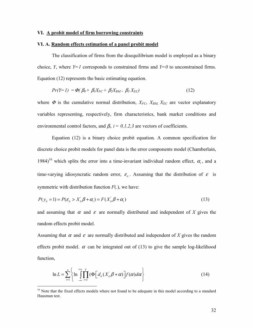
VI. A probit model of firm borrowing constraints

VI. A. Random effects estimation of a panel probit model

The classification of firms from the disequilibrium model is employed as a binary

choice, Y, where Y=1 corresponds to constrained firms and Y=0 to unconstrained firms.

Equation (12) represents the basic estimating equation.

Pr(Y=1) =Φ( β0 + β1XFC + β2XBM + β3 XEC) (12)

where Φ is the cumulative normal distribution, XFC, XBM, XEC are vector explanatory

variables representing, respectively, firm characteristics, bank market conditions and

environmental control factors, and βi, i = 0,1,2,3 are vectors of coefficients.

Equation (12) is a binary choice probit equation. A common specification for

discrete choice probit models for panel data is the error components model (Chamberlain,

1984)16

which splits the error into a time-invariant individual random effect, iα , and a

time-varying idiosyncratic random error, itε . Assuming that the distribution of ε is

symmetric with distribution function F(.), we have:

' '( 1) ( ) ( )it it it i it iP y P X F Xε β α β α= = > + = + (13)

and assuming that α and ε are normally distributed and independent of X gives the

random effects probit model.

Assuming that α and ε are normally distributed and independent of X gives the random

effects probit model. α can be integrated out of (13) to give the sample log-likelihood

function,

'

1 1

ln ln ( ( ) ( )Tn

it iti t

L d X f dβ α α α+∞

= =−∞

= Φ +

∑ ∏∫ (14)

16

Note that the fixed effects models where not found to be adequate in this model according to a standard

Hausman test.

33

where 2 1it itd y= − . This expression contains a univariate integral which can be

approximated by Gauss-Hermite quadrature. Assuming α ∼ 2(0, )N ασ ), the contribution

of each individual to the sample likelihood function is,

{ }2 2 2(1/ 2 ) exp( / 2 ) ( ) ( )itL g dα απσ α σ α α+∞

−∞

= −∫ (15)

where '

1

( ) ( ( )T

it itt

g d Xα β α=

= Φ + ∏ . Use the change of variables, 22 αα σ ζ= to give,

{ }2 2(1/ ) exp( ) (( 2 ) ) ( )iL g dαπ ζ σ ζ ζ+∞

−∞

= −∫ (16)

As it takes the generic form 2exp( ) ( )f dζ ζ ζ+∞

−∞

−∫ , this expression is suitable for Gauss-

Hermite quadrature and can be approximated as a weighted sum,

iL ∼ 2

1

(1/ ) (( 2 ) )m

j jj

w g aαπ σ=

∑ (17)

where the weights ( jw ) and abscissae ( ja ) are tabulated in standard mathematical

references and m is the number of nodes or quadrature points (Butler and Moffitt, 1982).

VI B. Probit results and marginal effects

The results of the probit model are shown in Table 10.17

The table reports both

the parameter estimates and the marginal effect of each explanatory variable on the

response probability. Marginal effects are reported in percentage points and computed at

17

The results correspond to a random effect model accounting for autocorrelation. An AR(1) process is

added to the random effects estimator to account for autocorrelation. The autocorrelation parameter (ρ) was

significant in all cases and, hence, we mainly rely on the results that account for autocorrelation. The

number of points employed in the Hermite quadrature was 20, although the results remain consistent to

other specifications.

34

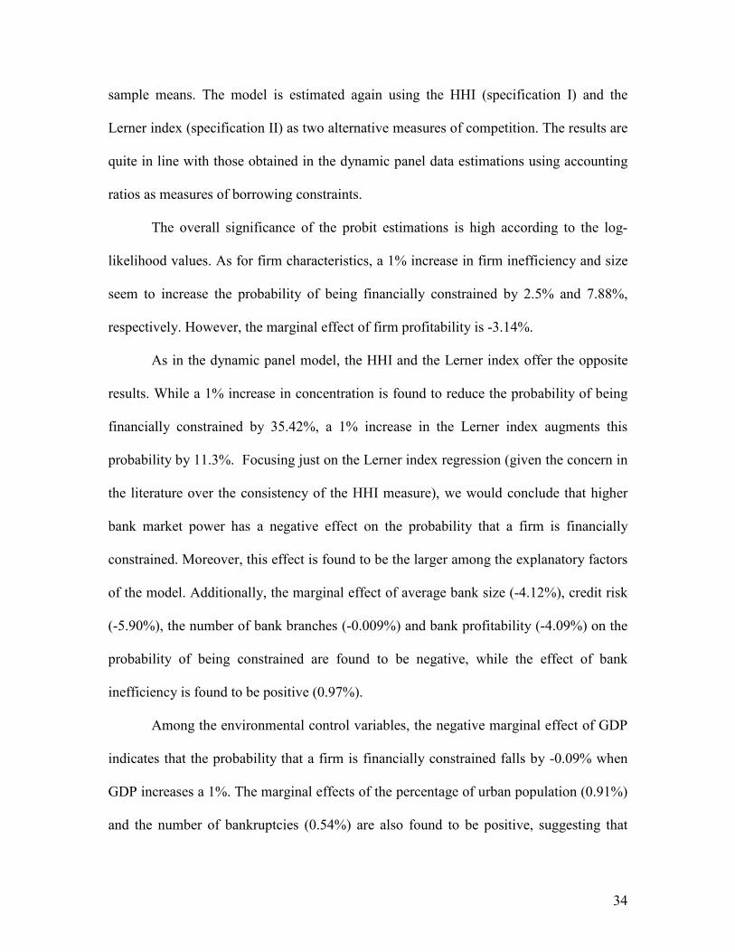
sample means. The model is estimated again using the HHI (specification I) and the

Lerner index (specification II) as two alternative measures of competition. The results are

quite in line with those obtained in the dynamic panel data estimations using accounting

ratios as measures of borrowing constraints.

The overall significance of the probit estimations is high according to the log-

likelihood values. As for firm characteristics, a 1% increase in firm inefficiency and size

seem to increase the probability of being financially constrained by 2.5% and 7.88%,

respectively. However, the marginal effect of firm profitability is -3.14%.

As in the dynamic panel model, the HHI and the Lerner index offer the opposite

results. While a 1% increase in concentration is found to reduce the probability of being

financially constrained by 35.42%, a 1% increase in the Lerner index augments this

probability by 11.3%. Focusing just on the Lerner index regression (given the concern in

the literature over the consistency of the HHI measure), we would conclude that higher

bank market power has a negative effect on the probability that a firm is financially

constrained. Moreover, this effect is found to be the larger among the explanatory factors

of the model. Additionally, the marginal effect of average bank size (-4.12%), credit risk

(-5.90%), the number of bank branches (-0.009%) and bank profitability (-4.09%) on the

probability of being constrained are found to be negative, while the effect of bank

inefficiency is found to be positive (0.97%).

Among the environmental control variables, the negative marginal effect of GDP

indicates that the probability that a firm is financially constrained falls by -0.09% when

GDP increases a 1%. The marginal effects of the percentage of urban population (0.91%)

and the number of bankruptcies (0.54%) are also found to be positive, suggesting that

35

higher demand sophistication and financial instability result in a higher probability of

firm credit rationing.

VII. Additional robustness checks: consistency of borrowing constraints and bank

competition measures

The empirical evidence shown in this study depends heavily on the validity of two

types of indicators: (i) financing constraints measures; (ii) competition measures. So far,

we have addressed concern about these indicators by using multiple measures of

financing constraints (i.e., a set of four accounting ratios and a classification from the

disequilibrium model) and two measures of market power. In this section we pursue

additional robustness checks.

With regard to the financing constraint measures, we consider three additional

caveats. As a first caveat, we follow Kaplan and Zingales (1997) and restrict the validity

of the “sales growth” measure. They show that controlling for high values of sales growth

seems to be an useful tool to control for “apparent” lower levels of financing constraints

(simply due to extraordinary and temporary high sales growth). Considering this potential

bias, we replicate the dynamic panel estimations including only those firms that exhibited

a sales growth rate lower that 30%. This restriction was applied not only to the equation

where sales growth was the dependent variable but also to the rest of accounting

measures (“trade credit/total liabilities”, “trade credit/tangible assets” and “loans/tangible

assets”). The results remain very similar to the original dynamic panel estimations18

.

Therefore, extraordinary sales growth levels are not found to introduce significant bias in

our results. Second, since the results of the disequilibrium model have shown more

18

These results are available upon request and are not shown here for simplicity.

36

variation across sectors than across regions, we examine the extent to which the industrial

structure of the region may affect the probability that a firm is financially constrained.

Additional dynamic panel and probit estimations were then undertaken eliminating those

firms belonging to the most and the least financially constrained sectors19

. None of the

conclusions on the determinants of firm borrowing constraints were modified according

to the results obtained.

A third caveat refers to a debate that has garnered considerable attention in the

firm financing literature. In particular, we examine the extent to which borrowing

constraints are correlated with investment-cash flow correlations. The relationship

between corporate investment and cash flow is, to a certain extent, a sort of a "black

box". While Fazzari et al. (2000) suggest that financing constraints grow along with

correlations between investment and cash-flow, Kaplan and Zingales (1997, 2000)

suggested that investment-cash flow correlations are not necessarily monotonic in the

degree of financing constraints. Importantly, most of the firms in our sample are non-

quoted corporations. Hines and Thaler (1995) and Kaplan and Zingales (2000) suggested

that investment-cash flow sensitivities can be, at least, partially caused by non-optimizing

behaviour by managers. This behaviour would be more frequent in non-quoted SMEs

since capital market discipline is not so strong in these firms. There is an alternative

methodology (Bond and Meghir, 1994) to compute cash-flow investment correlations in

unquoted firms, when the Tobin’s-q is not available as a measure of firm’s capital

performance. The methodology consists of an Euler equation:

19

The firms belonging to the following sectors were excluded: manufactures of food products and

beverages; manufactures of textiles and dressing; electricity, gas and water supply; construction; sale,

maintenance and repair of motor vehicles; hotels and restaurants; transport services .

37

Investmentt/capitalt-1 = α*Investmentt-1 + β*Investment2 + χ*Cash flowt/capitalt-1 +

δ*sales + +γ*debt2

The “investment” variable employed is the estimated value of coefficient “χ” is taken as

the cash-flow investment correlation. To use this methodology, we have employed the

same investment variable (Capital expenditures) employed by Kaplan and Zingales

(1997) and Fazzari et al. (2000). In order to compare the cash-flow investment

correlations with the level of financing constraints, the Euler equation has been estimated

for the four quartiles going from less constrained (quartile 1) to most constrained firms

(quartile 4) (using “trade credit/total liabilities” as an example),. The results are shown in

Table 11. Interestingly, the cash-flow investment correlations are monotonic. They

increase significantly from quartile 1 to quartile 2 and from quartile 2 to quartile 3.

However, they seem to maintain a very high value over the median (quartiles 3 and 4).

Therefore, we may, at least, assume that a monotonic relationship holds between cash

flow-investment correlation and firms financing constraints at least for firms below and

over the median value of “trade credit/total liabilities”. That is, in general our borrowing

constraints are correlated with investment-cash flow correlations in the predicted way.

The second set of additional robustness check refers to the consistency of

competition measures. Together with the HHI of bank deposits, various concentration

measures were considered. First of all, we substituted the HHI of bank deposits with the

one (CR1), three (CR3) and five (CR5) largest banks, respectively. The HHI was not

robust to alternative specifications. Only the CR3 measure appeared to be negatively and

significantly related to the financing constraint variables (as the HHI of bank deposits).

The HHI of bank loans and of bank total assets were also included as concentration

38

measures and only the former provided statistically significant results in line with those

of the HHI of bank deposits. The inconsistency of the concentration measures castes

some doubt on the accuracy of concentration as a measure of market power.

Various alternative variables were also tested as a robustness check for the Lerner

index. A general concern about the use of the Lerner index is the problem of endogeneity

since there are influences that may simultaneously affect both financing constraint

measures and the Lerner index, such as the business cycle or some bank characteristics.

As a first robustness check, only the numerator of this index – the mark-up of price over

marginal costs - was included as a dependent variable. The aim was to abstract both

prices and marginal costs (in levels) from business cycle influences, as in Maudos and

Fernández de Guevara (2004). While the price of total assets is influenced by business

cycle effects the net interest margin is not. The results were very similar to those obtained

using the Lerner index. A second alternative measure to the Lerner index was the ratio

“(interest revenue-interest expense)/total assets”. This ratio proxies pricing behavior in

both loan and deposit markets while the Lerner index is more inclusive (including all

earning assets). As in the case of the Lerner index, interest margins over total assets were

found to be positively and significantly related to borrowing constraints. A third

robustness check for the Lerner index consists of including the price of total assets and

marginal costs separately as explanatory variables. As expected, prices were found to be

positively and significantly related to borrowing constraints while marginal costs were

negatively and significantly related to the borrowing constraints variables. An additional

concern with regard to endogeneity is the possible correlation between the Lerner index

and other bank market characteristics such as bank profitability. However, the correlation

39

coefficient between both variables (0.19) is too low as to impose separability in the

estimation of the effects of bank market power and profitability in the regressions. The

endogeneity of the Lerner index was also examined by ‘instrumenting’ the variable. In

particular, the price variable in both the numerator and the denominator of the Lerner

index was replaced by a ‘predicted value’ of this price. The predictions were obtained

from a simple regression of the price variable of the level of bank capitalization (capital

to total assets ratio) which is found to be correlated with bank prices but not with

financing constraints20

. The ‘instrumented’ Lerner index offer very similar results to

those obtained using the standard Lerner index variable.

Finally, an additional test was undertaken to analyze the stability of the estimated

parameters -in the dynamic panel equations- over time. Therefore, separate yearly cross-

section OLS regressions were undertaken as a robustness check for dynamic panel

estimations. The coefficients of all the explanatory factors remain relatively stable over

time21

with the HHI of bank deposits being the main exception. In particular, the HHI

was found to be positively and significantly related to borrowing constraints in 1994,

1995 and 1996, it was not statistically significant in 1997 and only achieved a negative

sign from 1998 onwards. This result also suggests that the econometric outcomes from

concentration measures are frequently spurious and that changes in bank market structure

in recent years are better captured by looking at price to marginal costs indicators such as

the Lerner index.22

20

The correlation coefficient between bank capital and bank prices is found to be high and positive (0.7),

while the correlation of bank capital on the financing constraint measures was not higher than 0.13 in any

case. 21

With poorer economic significance compared to dynamic panel outcomes. 22

The overtime econometric inconsistency of the HHI as an explanatory variable of competitive behavior

has been also shown for the US by Moore (1998).

40

VIII. Conclusions

Corporate financing is one of the key pillars of the nexus between the financial

sector and economic growth. For SMEs banks appear to play a particularly relevant role

in providing external financing, since these firms are much more dependent on bank

financing than their larger counterparts. This study analyzes a potentially critical factor in

SME lending, the effect of bank market competition on firm borrowing constraints. Most

previous studies of SME financing have confined their analysis to concentration

indicators such as the Herfindahl Hisrchman index (HHI) as proxies of banking market

competition. However, several studies have suggested that concentration measures are

spurious indicators of bank market power and that other alternative measures based on

direct estimations of prices and marginal costs such as the Lerner index are more accurate

indicators of bank competition.

The relationship between bank competition and firm financing has been studied in

the context of two main competing hypotheses. The market power view holds that

concentrated banking markets are associated with less credit availability and a higher

price for credit. However, an alternative view, the information hypothesis that has

emerged during the last decade, argues that competitive banking markets can weaken

relationship-building by depriving banks of the incentive to invest in soft information.

Therefore, according to the information hypothesis, higher bank market power will

reduce firm financing constraints. However, most of the studies that have found empirical

support for the information hypothesis have relied on the HHI concentration indicators.

41

In addition, most of them have studied this issue on data from the US where relationship

lending is just one lending technology among many others.

This study offers new evidence on the relationship between bank market

competition and firm financing constraints. Employing a large sample of firms and

combining firm level data with bank level conditions in the markets where each firm

operates, both concentration (HHI) and price to marginal costs indicators (specifically,

the Lerner index) are analyzed as measures of bank competition. These measures are

included along with other firm level, bank market and environmental control factors as

determinants of firm borrowing constraints. Similarly, various measures of firm

borrowing constraints are considered, including various accounting indicators and a

classification from a disequilibrium model of bank lending. Our results are consistent

across alternative specifications of borrowing constraints. In addition, they are consistent

across alternative specifications of market power. However, they are not consistent

across measures of bank market power. Specifically, the HHI and the Lerner index offer

consistently opposite results. However, we find that the Lerner index is a considerably

more accurate measure of competition. This lack of accuracy is in line with other

findings in the banking literature that shed doubt on the strength of concentration as

measure of market power (e.g., Berger, 1995; Rhoades, 1995; Jackson 1997; Hannan,

1997; Dick, 2005). Taking the Lerner index as the more reliable reference, our results

show that bank market power increases firm financing constraints. Moreover, probit

model results reveal that market power has the greater marginal effect on the probability

that a firm is financially constrained among the posited set of explanatory factors. All in

all, we argue that our results provide more support for the market structure hypothesis in

42

bank lending relationships. Our findings also raise doubts about the value of relying

exclusively, or even primarily, on concentration indicators as measures of bank

competitive conditions in studies of bank-firm relationships.

43

References

Almeida, H. and M. Campello (2004): Financial Constraints, Asset Tangibility, and Corporate Investment, Working Paper, New York University and University of Illinois.

Angelini, P. and N. Cetorelli (1999): Bank Competition and Regulatory Reform: The Case of the Italian Banking Industry, Working Paper, Research Department, Federal

Reserve Bank of Chicago, December (WP-99-32).

Arellano, M. and S. Bond (1991): “Some tests of specification for panel data: Monte

Carlo evidence and an application to employment equation”, Review of Economic Studies 58: 277-287.

Arellano M. and O. Bover (1995): “Another Look at the Instrumental-Variable Estimation

of Error-Components Models,” Journal of Econometrics, 68: 29-51.

Atanasova, C.V. and N. Wilson (2004): ‘Disequilibrium in the UK Corporate Loan

Market’, Journal of Banking and Finance, 28: 595-614.

Avery, R. B. and A. N. Berger (1991a) "Loan Commitments and Bank Risk Exposure"

Journal of Banking and Finance, 15: 173-92.

Avery, R., Bostic, R. and K. Samolyk (1998): “The Role of Personal Wealth in Small

Business Finance,” Journal of Banking and Finance, 22: 1019-1061.

Bakker, M. H. R., Klapper, L. and G. F. Udell (2004): Financing Small- and Medium-Size Enterprises with Factoring: Global Growth in Factoring—and Its Potential in Eastern Europe. Washington, DC: World Bank.

Becchetti, L. and J. Sierra (2003): “Bankruptcy risk and productive efficiency in

manufacturing firms”, Journal of Banking and Finance, 27: 2099-2120

Berg, S. A., and M. Kim (1994): “Oligopolistic Interdependence and the Structure of

Production in Banking: An Empirical Evaluation”, Journal of Money, Credit, and Banking, 26: 309-22.

Berger, A. N. (1995): “The Profit Structure Relationship in Banking. Tests of Market-

Power and Efficient-Structure Hypotheses”, Journal of Money, Credit, and Banking 27:

404-431.

Berger, A. N., (2004): Potential Competitive Effects of Basel II on Banks in SME Credit Markets in the United States, Finance and Economics Discussion Series paper 2004-12,

Board of Governors of the Federal Reserve System.

44

Berger, A. N. and T. Hannan (1989): “The Price-Concentration Relationship in Banking”.

The Review of Economics and Statistics, Volume 71, Issue 2 291-299.

Berger, A.N., Hasan, I., Klapper, L.F. (2004): “Further evidence on the link between

finance and growth: An international analysis of community banking and economic

performance”, Journal of Financial Services Research 25: 169-202.

Berger, A. N. and G. F. Udell (1990): “Collateral, loan quality, and bank risk,” Journal of Monetary Economics, 25: 21-42.

Berger, A.N. and G. F. Udell (1992): “Some evidence on the empirical significance of

credit rationing” Journal of Political Economy, 100: 1047-1077.

Berger, A. N. and G. F. Udell (1995): “Relationship lending and lines of credit in small

firm finance”, Journal of Business, 68: 351-381.

Berger, A. N. and G. F. Udell (1996). “Universal Banking and the Future of Small

Business Lending,” in by A. Saunders and I. Walter (eds.): Universal Banking: Financial System Design Reconsidered, Chicago: Irwin Professional Publishing: 558-627.

Berger, A.N. and G.F. Udell (1998): “The economics of small business finance: The roles

of private equity and debt markets in the financial growth cycle,” Journal of Banking and Finance, 22: 613-673

Berger, A. N., and G. F. Udell (2002): “Small Business Credit Availability and

Relationship Lending: The Importance of Bank Organizational Structure,” Economic Journal,112: 32-53.

Berger, A.N. and G.F. Udell (forthcoming): “A More Complete Conceptual Framework

for SME Finance”, Journal of Banking and Finance, forthcoming.

Berger, A. N., Rosen, R.J. and G. F. Udell (forthcoming): “Does Market Size Structure

Affect Competition? The Case of Small Business Lending”, Journal of Banking and Finance, forthcoming.

Berger, A. N., Demirguc-Kunt, A., Levine, R. and J. G. Haubrich (2004): “Bank

Concentration and Competition: An Evolution in the Making’, Journal of Money, Credit, and Banking, 36: 433-451.

Berger, A, N., Miller, N. H., Petersen, M. A., Rajan, R. and J. Stein (2005): "Does

function follow organizational form? Evidence from the lending practices of large and

small banks" Journal of Financial Economics, 76: 237-269

Berkovitch, E. and S. I. Greenbaum (1990): “The Loan Commitment as an Optimal

Financing Contract”, Journal of Financial and Quantitative Analysis 26: 83-95.

45

Besanko, D. and A. Thakor, (1987a): “Collateral and rationing: Sorting Equilibria in

monopolistic and competitive credit markets,” International Economic Review, 28: 671-

89.

Besanko, D. and A. Thakor (1987b): “Competitive equilibrium in the credit market under

asymmetric information” Journal of Economic Theory, 71: 291-99.

Bester, H. (1985): "Screening vs. Rationing in Credit Markets with Imperfect

Information.'' American Economic Review, 75: 850-855.

Blundell, R., Bond, S. and F. Windmeijer (2000): Estimation in dynamic panel models: Improving on the performance on the standard GMM estimator, The Institute for Fiscal

Studies, WP 00/12.

Bond, S., and C. Meghir (1994) “Dynamic investment models and the firm’s financial

policy.”, Review of Economic Studies, 61:197-222.

Boot, A. and A. Thakor (2000): “Can Relationship Banking Survive Competition?”,

Journal of Finance, 55: 679-713.

Boot, A. W. A., Thakor, A.V. and G. F. Udell (1987): “Competition, Risk Neutrality and

Loan Commitments”, Journal of Banking and Finance 11: 449-471.

Boot, A., Thakor A. and G. F. Udell (1991): “Secured lending and default risk:

Equilibrium analysis and policy implications and empirical results” Economic Journal, 101: 458-72.

Boyd, J. and E.C. Prescott (1986): "Financial Intermediary-Coalitions," Journal of Economic Theory, 38: 211-232.

Butler, J. and R. Moffitt, R. (1982): “A computationally efficient quadrature procedure

for the one-factor multinomial probit model”, Econometrica, 50: 761-764.

Caminal, R., and C. Matutes (2002): “Market Power and Banking Failures”, International Journal of Industrial Organization 20: 1341-1361.

Carbó, S., Humphrey, D. and F. Rodríguez (2003): “Deregulation, bank competition and

regional growth”, Regional Studies 37: 227-237.

Carter, D. A., and J. E. McNulty (2005): Deregulation, Technological Change, and the Business Lending Performance of Large and Small Banks, mimeo.

Carter, D. A., McNulty, J.E. and J. A. Verbrugge (2004): “Do Small Banks have an

Advantage in Lending? An Examination of Risk-adjusted Yields on Business Loans at

Large and Small Banks”, Journal of Financial Services Research, 25: 233-252.

46

Cetorelli, N. and M. Gambera (2001): “Banking Market Structure, Financial Dependence

and Growth: International Evidence from Industry Data”, Journal of Finance, 56: 617-

648.

Chamberlain, G. (1984): “Panel data”, in Griliches, Z. and M.D. Intrilgator (eds.),

Handbook of Econometrics, North Holland:1247-1318.

Chan, Y.S. and G. Kanatas (1985): “Asymmetric valuation and the role of collateral in

loan agreements”, Journal of Money, Credit and Banking, 17: 85-95.

Cole, R. (1998). ‘The importance of relationships to the availability of credit.’ Journal of Banking and Finance, 22: 959-77.

Cole, R. A., Goldberg, L.G. and L. J. White (2004): “Cookie-cutter versus character: The

Micro Structure of Small Business Lending by Large and Small Banks.” Journal of Financial and Quantitative Analysis, 39: 227-251.

De Mello, J.M.P. (2004): Market Power and Availability of Credit: An Empirical Investigation of the Small Firms Credit Market, mimeo.

Degryse, H., and P. Cayseele (2000): ‘Relationship lending within a bank-based system:

Evidence from European small business data.’ Journal of Financial Intermediation, 9:

90-109.

Dell'Arricia, G. and R. Marquez (2004): “Information and Bank Credit Allocation”,

Journal of Financial Economics, forthcoming.

Demirgüç-Kunt, A. and V. Maksimovic (1998): “Law, finance and firm growth”, Journal of Finance, 53: 2107-2137.

Demirgüç-Kunt, A. and V. Maksimovic (1999): “Institutions, Financial Markets and Firm

Debt Maturity,” Journal of Financial Economics, 54, 66-97 .

Demirguc-Kunt, A., and V. Maksimovic (2001): Firms as Financial Intermediaries: Evidence from Trade Credit Data, Working Paper, World Bank and the University of

Maryland.

Dick, A.A. (2005): "Market Size, Service Quality and Competition in Banking", Journal of Money, Credit and Banking, forthcoming.

Elsas, R. (2005): “Empirical Determinants of Relationship Lending”, Journal of Financial Intermediation, 14: 32-57.

Elsas, R. and J.P. Krahnen (1998): “Is relationship lending special? Evidence from credit-

file data in Germany”, Journal of Banking and Finance, 22: 1283-1316.

Evans, D. and B. Jovanovic (1989): “An Estimated Model of Entrepreneurial Choice

47

Under Liquidity Constraints”, Journal of Political Economy, 97: 808-827.

Fazzari, S. M., Hubbard, R. G. and B. C. Petersen (2000): Financing Constraints and Corporate Investment: Response to Kaplan and Zingales" NBER Working Papers 5462.

Gersovitz, M. (1980): “On classification probabilities for the disequilibrium model”,

Journal of Econometrics, 14: 239–246.

Gorton, G., and J. Kahn (1997): The design of bank loan contracts, collateral, and renegotiation, University of Pennsylvania Working Paper.

Greenwald, B. and J. E. Stiglitz (1986): “Externalities in Economies with Imperfect

Information and Incomplete Markets,” Quarterly Journal of Economics , May: 229-264.

Hannan, T. H. (1991): “Bank commercial loan markets and the role of market structure:

Evidence from surveys of commercial lending”, Journal of Banking and Finance, 15:

133-149.

Hannan, T.H. (1997): Market share inequality, the number of competitors, and the HHI:

An examination of bank pricing, Review of Industrial Organization 12: 23-35.

Hannan, T.H. y A. Berger (1991): “The Rigidity of Prices: Evidence from the Banking

Industry”, American Economic Review, 81: 938-945.

Harhoff, D. and T. Körting, T. (1998): “Lending relationships in Germany: Empirical

results from survey data”, Journal of Banking and Finance, 22: 1317-54.

Haynes, G., Ou, C. and R. Berney (1999): “Small Business Borrowing from Large and

Small Banks” Proceedings of the Federal Reserve Bank of Chicago March: 287-293

Hines, J.R. Jr. and R. Thaler (1995): “The flypaper effect”, Journal of Economic Perspectives, 9: 217-226.

Houston, J.F., and C. James (1998): “Do bank internal capital markets promote

lending?”, Journal of Banking and Finance, 22: 899-918.

Jackson, W. (1997): “Market structure and the speed of adjustment: Evidence of

nonmonotonicity”, Review of Industrial Organization, 12: 37-57.

James, C. (1987): "Some Evidence on the Uniqueness of Bank Loans," Journal of Financial Economics, 19: 217-235.

Jayaratne, J., and J.D. Wolken (1999): “How important are small banks to small business

lending? New evidence from a survey to small businesses” Journal of Banking and Finance 23: 427-458.

48

John, K., A. Lynch, and M. Puri (2003): “Credit ratings, collateral and loan

characteristics: Implications for yield”, Journal of Business, 76: 371-410.

Kanatas, G. (1987): “Commercial Paper, Bank Reserve Requirements, and the

Informational Role of Loan Commitments”, Journal of Banking and Finance, 11: 425-

448.

Kaplan, S. and L. Zingales, 1997, “Do Financing Constraints Explain why Investment is

Correlated with Cash Flow?” Quarterly Journal of Economics, 112, pp. 169-215.

Klapper, L., (1998): Short-term collateralization: Theory and evidence, New York

University working paper.

Lamont, O., C. Polk and J. Saá-Requejo (2001): “Financial constraints and stock returns”,

Review of Financial Studies, 14: 529-54.

Lel, U. and G. Udell (2002): Financial Constraints, Start-up Firms and Personal Commitments, mimeo.

Lummer, S. L., and J.J. McConnell (1989). "Further Evidence on the Bank Lending

Process and the Capital Market Response to Bank Loan Agreements," Journal of Financial Economics, 25: 99-122.

Maddala, G. S. (1983): Limited-Dependent and Qualitative Variables in Econometrics, Cambridge: Cambridge University Press.

Maddala, G. S. and F.D. Nelson (1974): “Maximum likelihood methods for models of

markets in disequilibrium”, Econometrica 42: 1003–1030.

Maudos, J. and J. Fernandez de Guevara (2004): “Factors explaining the interest margin

in the banking sectors of the European Union’, Journal of Banking and Finance, 28:

2259-2281.

Melnik, A., S. E. Plaut (1986): “Loan Commitment Contracts, Terms of Lending, and

Credit Allocation” Journal of Finance, 41: 425-435.

Mester, Loretta J., Leonard I. Nakamura, and Micheline Renault, “Checking Accounts

and Bank Monitoring,” Working Paper, Federal Reserve Bank of Philadelphia (October

1998).

Miwa, Y., J.M. Ramseyer (2005). “Trade Credit, Bank Loans, and Monitoring: Evidence

from Japan.” University of Tokyo Working Paper.

Moore, R. R. (1998), “Concentration, Technology, and Market Power in Banking: Is

Distance Dead?”, Financial Industry Studies, Federal Reserve Bank of Dallas, December,

págs.1-24.

49

Morgan, D.P. (1994): “Bank credit commitments, credit rationing, and monetary policy”,

Journal of Money, Credit, and Banking, 26: 87-101.

Morgan, D. P. (1998): “The Credit Effects of Monetary Policy: Evidence Using Loan

Commitments.” Journal of Money Credit and Banking, 30: 102-118.

Ogawa, K., K. Suzuki (2000): “Uncertainty and investment: some evidence from the

panel data of Japanese manufacturing firms”, Japanese Economic Review, 51: 170-192.

Ongena, S., and D.C. Smith (2001): “The duration of bank relationships”, Journal of Financial Economics, 61: 449-475.

Petersen, M. A. and R. G. Rajan (1992): The Benefits of Firm-Creditor Relationships: Evidence from Small Business Data" University of Chicago Working Paper no. 362.

Petersen, Ml A. and R. G. Rajan (1994): "The Benefits of Lending Relationships:

Evidence from Small Business Data", Journal of Finance, 49: 3-37.

Petersen, M.A. and R.G. Rajan (1995): “The effect of credit market competition on

lending relationships”, Quarterly Journal of Economics 110: 407-443.

Rajan, R. and L. Zingales (1998): “Financial dependence and growth”, American Economic Review 88: 559-586.

Rhoades, S. A. (1995): "Market Share Inequality, the HHI, and Other Measures of the

Firm-Composition of A Market", Review of Industrial Organization: 657-674.

Ribon, S. and O. Yosha (1999): Financial Liberalization and Competition in Banking: An Empirical Investigation, Tel Aviv University, Working Paper, 23-99.

Roberts, M. (1984): “Testing oligopolistic behavior”, International Journal of Industrial Organization, 2: 367–383.

Schiantarelli, F. (1995): “Financial Constraints and Investment: A Critical Review of

Methodological Issues and International Evidence,” in J. Peek and E. Rosengren (eds.),

Federal Reserve Bank of Boston Conference Series No. 39.

Schmalensee, R. (1989): “Inter-industry Studies of Structure and Performance”, in R.

Schmalensee and R.D. Willig (eds.), Handbook of Industrial Organisation, 2: 951-1009.

North-Holland, Amsterdam.

Scott J.A. and W.C. Dunkelberg (2005): "Bank Mergers and Small Firm Financing”,

Journal of Money, Credit and Banking, forthcoming.

50

Shaffer, S. (1993): “A test of competition in Canadian Banking”, Journal of Money, Credit and Banking, 25: 49-61

Sharpe, S. A. (1990): “Asymmetric information, bank lending and implicit contracts: A

stylized model of customer relationships”, Journal of Finance, 55: 1069-1087.

Shikimi, M. (2005): Do Firms Benefit from Multiple Banking Relationships? Evidence from Small and Medium-Sized Firms in Japan, Discussion Paper Series, nº70.

Hitotsubashi University Research Unit for Statistical Analysis in Social Sciences.

Smith, C. and J. Warner (1979): “On financial contracting: an analysis of bond

covenants”, Journal of Financial Economics, 7: 117-161.

Sofianos, G., Wachtel, P. and A. Melnik (1990): “Loan Commitments and Monetary

Policy,” Journal of Banking and Finance, 14: 677-89.

Stein, J. C. (2002), “Information Production and Capital Allocation: Decentralized versus

Hierarchical Firms” Journal of Finance, 57: 1891-1921.

Stiglitz, J.E. and A. Weiss (1981): “Credit rationing in markets with imperfect

information”. American Economic Review, 71:393-410.

Stulz, R. and H. Johnson (1985): “An analysis of secured debt”, Journal of Financial Economics, 14: 501-512.

Swary, I. and G.F. Udell (1988): Information Production and the Secured Line of Credit, New York University working paper (March).

Thakor, A. V. and G. F. Udell (1987): “An Economic Rationale for the Pricing

Structure of Bank Loan Commitments”, Journal of Banking and Finance 11: 271-289.

Welch, I. (1997): “Why is bank debt senior? A theory of asymmetry and claim priority

based on influence costs”, Review of Financial Studies, 10: 1203-1236.

Zarutskie, R. (2003): Does Bank Competition Affect How Much Firms Can Borrow? New Evidence from the U.S., presented at Corporate Governance: Implications

for Financial Services Firms, 39th Annual Conference on Bank Structure and

Competition, Chicago, May 7-9, 2003.

51

Appendix A: Translog function to compute marginal costs in regional bank markets

Bank marginal costs are computed using a single output (total assets) translog cost

function with two cost share equations over 1994-2002:

[ ]ln ' + ' + ' (ln ) (ln )

(- ) (ln ) ln ln ( - )(ln )

ln + ln ( ) ( ) ln

ln (ln ) (- ) ln (ln

α α φ δ φ η ρ ρ

ρ ρ β β λ λ

γ γ γ γ γ γ

γ γ γ

= + + + +

+ − + + + −

+ + + + +

+ + −

22

0 1 11 1 1 11 1 12 2

11 12 3 1 1 2 2 1 2 3

2 2 2

11 1 22 2 11 12 12 22 3

12 1 2 11 12 1

1 1

2 2

1

1

2

t t tTC Q t Q t Q t Q R Q R

Q R R R R

R R R

R R R ) ( ) ln (ln )

'ln 'ln 'ln

γ γ

µ µ µ ε

+ −

+ + + +

3 12 22 2 3

1 1 2 2 3 3t t t

R R R

t R t R t R

[A1]

1SH ln ln (- - ) 'ρ β γ γ γ γ µ= + + + + +11 1 11 1 12 2 11 12 3 1kQ R R R t [A2]

2 12 2 22 2 12 1 22 12 3 2ln ln (- - ) 'ρ β γ γ γ γ µ= + + + + + kSH Q R R R t [A3]

where the standard symmetry, summation, and cross-equation restrictions are imposed and lnTC

is the log of total operating and interest cost; lnQ is the log of the value of total assets (an

indicator of total banking output); lnRi is the log of each one of the three input prices (deposit and

other funding interest rate, average price of labor, and the average price of physical capital); SH1

and SH2 are the cost share equations of deposit and other funding interest expense and labor cost

share (the cost share of physical capital is excluded); t is a time dummy reflecting the effects of

technical change on costs over time.

52

Appendix B: Computing probabilities from the disequilibrium model of firm

financing constraints

According to the results from the disequilibrium model in section V.B., a firm is

defined as financially constrained in year t if the probability that the desired amount of

bank credit in year t exceeds the maximum amount of credit available in the same year is

greater than 0.5. Following Gersovitz (1980), the probability that firm will face a

financial constraint in year is derived as follows:

Pr( ) Pr( )d d s s

d s d d d s s s it itit it it it it it

X Xloan loan X u X u

β ββ β

σ

−> = + > + = Φ

(B1)

where ditX and s

itX denote the variables that determine firms’ loan demand and the

maximum amount of credit available to firms, respectively. The error terms are assumed

to be distributed normally, 2 var( )d sit itu uσ = − , and Φ (.) is a standard normal distribution

function. Since ( )d d dit itE loan X β= and ( )s s s

it itE loan X β= , Pr( ) 0.5d sit itloan loan> > , if and

only if ( ) ( )d sit itE loan E loan> .

53

Table 1. Sample composition by region an sector REGION FIRMS OBSERVATIONS

ANDALUSIA 1.830 16.470

ARAGON 1.810 16.290

ASTURIAS 905 8.145

BALEARIC ISLANDS 781 7.029

CANARY ISLANDS 259 2.331

CANTABRIA 173 1.557 CASTILE LA MANCHA 1.750 15.750 CASTILE AND LEÓN 963 8.667 CATALONIA 8.767 78.903 COMUNIDAD VALENCIANA 3.640 32.760 EXTREMADURA 648 5.832 GALICIA 1.800 16.200

MADRID 3.660 32.940

MURCIA 756 6.804

NAVARRA 838 7.542

BASQUE COUNTRY 1.816 16.344

RIOJA 501 4.509

SECTOR FIRMS REGIONS

MANUFACTURES OF FOOD PRODUCTS AND BEVERAGES 2583 23247

MANUFACTURES OF TEXTILES AND DRESSING 1917 17253 MANUFACTURES OF WOOD, PAPER, PRINTING AND RECORDED MEDIA PRODUCTS 1564 14076 MANUFACTURES OF CHEMICAL, PLASTIC, MINERAL AND METAL PRODUCTS 3296 29664 MANUFACTURES OF MACHINERY AND EQUIPMENT AND TRASNSPORT VEHICLES 1947 17523

MANUFACTURES OF FURNITURE AND RECYCLING 513 4617

ELECTRICITY, GAS AND WATER SUPPLY 78 702

CONSTRUCTION 4428 39852

SALE, MAINTENANCE AND REPAIR OF MOTOR VEHICLES 1339 12051

WHOLESALE TRADE AND COMISSION TRADE 6439 57951

HOTELS AND RESTAURANTS 2484 22356

TRANSPORT SERVICES 1272 11448

REAL STATE ACTIVITIES 2236 20124

RENTING OF MACHINERY AND EQUIPMENT 112 1008

COMPUTER AND RELATED ACTIVITIES 203 1827

OTHER RETAIL TRADE PRODUCTS AND SERVICES 471 4239

OTHER 15 135

TOTAL 30.897 278.073

54

Table 2. MEAN VALUES OF THE POSITED VARIABLES OVER TIME (1994-2002)

1994 1995 1996 1997 1998 1999 2000 2001 2002 PERIOD

Bank market power

HHI bank deposits 0.12083 0.11733 0.11701 0.11356 0.10437 0.09645 0.08936 0.08314 0.07772 0.10220

Lerner index 0.2102 0.2304 0.2403 0.2419 0.2412 0.2517 0.2532 0.2637 0.2641 0.2488

Other bank market characteristics

Average bank size 8.0247 8.0928 8.3265 8.4085 8.4985 8.5123 8.6985 8.7158 8.8236 8.4215

Bank credit risk 0.03352 0.02545 0.01059 0.00625 0.00232 0.00051 0.000223 0.00013 0.000114 0.00879

Number of bank branches

3348 3450 3544 3590 3664 3702 3700 3687 3657 3594

Bank profitability 0.00927 0.01125 0.01363 0.01819 0.02543 0.0182 0.0253 0.0331 0.0288 0.02035

Bank inefficiency 0.71256 0.71053 0.70552 0.70523 0.6944 0.62015 0.6253 0.61002 0.56823 0.66133

Firm characteristics

Trade credit/total liabilities

0.34166 0.34326 0.34234 0.35104 0.3498 0.34754 0.35155 0.34383 0.34530 0.34626

Sales growth 0.38842 0.4721 0.6258 0.69692 0.71532 0.76181 0.73725 0.7825 0.91303 0.67702

Trade credit/tangible assets

0.42586 0.43988 0.42824 0.44007 0.41583 0.41055 0.44201 0.43218 0.43020 0.43322

Loans/tangible assets 0.21152 0.21337 0.20185 0.23597 0.22565 0.22219 0.23098 0.22436 0.22307 0.22688

Firm inefficiency 0.86954 0.85442 0.82546 0.85517 0.83102 0.7858 0.8337 0.8882 0.81483 0.83979

Firm profitability 0.0711 0.07656 0.07286 0.07116 0.07601 0.078 0.07135 0.06584 0.05432 0.07080

Firm size 13.73 13.78 13.84 13.93 14.03 14.12 14.23 14.29 14.33 14.03

Environmental

regional control

variables

GDP 41811 43643 44964 46400 48099 54074 52520 54016 55437 48996

Taxation 0.21814 0.2152 0.2183 0.2163 0.2258 0.2352 0.1925 0.1935 0.2025 0.21305

Percentage urban population

0.51252 0.52685 0.53713 0.53208 0.5412 0.5518 0.562 0.5727 0.5834 0.54663

Number of bankrupticies

16 14 15 15 10 13 9 4 3 11

55

Table 3. SMEs Financing constraints and firm, bank market and

environmental conditions (I). Dynamic panel data results.

p-values in parenthesis

Dependent variable (financial constraint)

Trade credit/(total

liabilities) Sales growth

(I) (II) (I) (II)

Constant -5.0092***

(0.000)

-5.3803***

(0.000)

-4.9957***

(0.000)

-5.0989***

(0.000)

Lagged dependent variable -1.7410***

(0.000)

-1.1637***

(0.000)

-0.28255

(0.383)

-0.56834***

(0.000)

Bank market power

HHI bank deposits -24.4223***

(0.000) -

18.3555***

(0.000) -

Lerner index - 0.0716***

(0.000) -

-37.7462**

(0.015)

Other bank market

characteristics

Average bank size -0.28390***

(0.000)

-0.06542***

(0.000)

0.29065***

(0.000)

0.34853***

(0.000)

Bank credit risk -8.1582***

(0.000)

-27.1408***

(0.000)

-8.4058

(0.205)

1.28231

(0.910)

Number of bank branches -0.0036***

(0.000)

-0.00558***

(0.000)

0.00347***

(0.003)

0.0057***

(0.000)

Bank profitability -4.2153***

(0.000)

-3.0651**

(0.015)

-1.7013***

(0.000)

-0.7377***

(0.003)

Bank inefficiency 0.0399***

(0.000)

0.04575***

(0.008)

-0.0254***

(0.000)

-0.03408***

(0.004)

Firm characteristics

Firm inefficiency -0.02573

(0.172)

0.0586**

(0.046)

-0.0513

(0.675)

-0.05244

(0.488)

Firm profitability 0.0929

(0.329)

-0.06610*

(0.054)

-1.5242

(0.132)

2.5287

(0.325)

Firm size 0.12027***

(0.000)

0.38549***

(0.000)

-0.2625**

(0.012)

-0.45281**

(0.022)

Environmental regional control

variables

GDP -0.35E-05***

(0.000)

-0.25E-05***

(0.000)

0.10E-05**

(0.021)

0.23E-05***

(0.000)

Taxation -0.00014

(0.670)

0.00027**

(0.022)

-0.0059*

(0.068)

-0.0030*

(0.090)

Percentage urban population 2.8449***

(0.000)

9.9921***

(0.000)

-12.2065***

(0.000)

-5.5814***

(0.002)

Number of bankrupticies 0.06977***

(0.000)

0.09627***

(0.000)

-0.0345***

(0.008)

-0.06417***

(0.008)

F-statistic 0.0166 0.015 0.021 0.020

Sargan test 0.137 0.163 0.131 0.129

Observations 278.073 278.073 278.073 278.073

Number of firms 30.897 30.897 30.897 30.897

* Statistically significant at 10% level ** Statistically significant at 5% level *** Statistically significant at 1% level

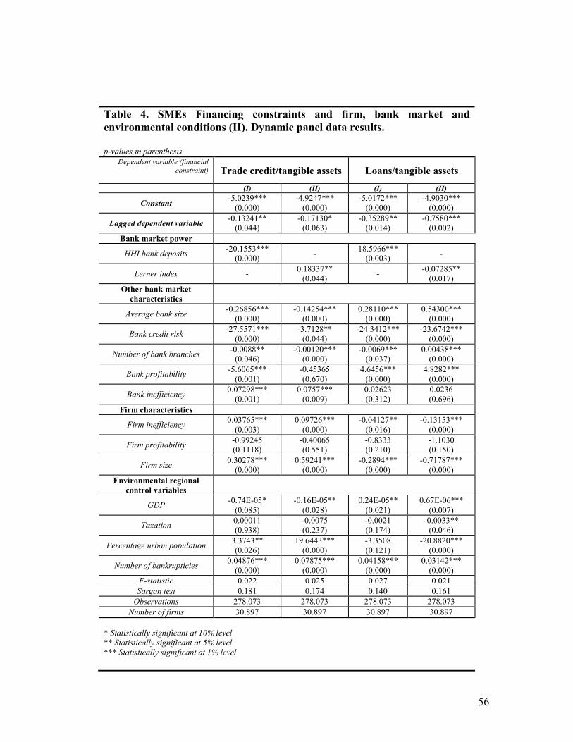
56

Table 4. SMEs Financing constraints and firm, bank market and

environmental conditions (II). Dynamic panel data results.

p-values in parenthesis

Dependent variable (financial constraint)

Trade credit/tangible assets Loans/tangible assets

(I) (II) (I) (II)

Constant -5.0239***

(0.000)

-4.9247***

(0.000)

-5.0172***

(0.000)

-4.9030***

(0.000)

Lagged dependent variable -0.13241**

(0.044)

-0.17130*

(0.063)

-0.35289**

(0.014)

-0.7580***

(0.002)

Bank market power

HHI bank deposits -20.1553***

(0.000) -

18.5966***

(0.003) -

Lerner index - 0.18337**

(0.044) -

-0.07285**

(0.017)

Other bank market

characteristics

Average bank size -0.26856***

(0.000)

-0.14254***

(0.000)

0.28110***

(0.000)

0.54300***

(0.000)

Bank credit risk -27.5571***

(0.000)

-3.7128**

(0.044)

-24.3412***

(0.000)

-23.6742***

(0.000)

Number of bank branches -0.0088**

(0.046)

-0.00120***

(0.000)

-0.0069***

(0.037)

0.00438***

(0.000)

Bank profitability -5.6065***

(0.001)

-0.45365

(0.670)

4.6456***

(0.000)

4.8282***

(0.000)

Bank inefficiency 0.07298***

(0.001)

0.0757***

(0.009)

0.02623

(0.312)

0.0236

(0.696)

Firm characteristics

Firm inefficiency 0.03765***

(0.003)

0.09726***

(0.000)

-0.04127**

(0.016)

-0.13153***

(0.000)

Firm profitability -0.99245

(0.1118)

-0.40065

(0.551)

-0.8333

(0.210)

-1.1030

(0.150)

Firm size 0.30278***

(0.000)

0.59241***

(0.000)

-0.2894***

(0.000)

-0.71787***

(0.000)

Environmental regional

control variables

GDP -0.74E-05*

(0.085)

-0.16E-05**

(0.028)

0.24E-05**

(0.021)

0.67E-06***

(0.007)

Taxation 0.00011

(0.938)

-0.0075

(0.237)

-0.0021

(0.174)

-0.0033**

(0.046)

Percentage urban population 3.3743**

(0.026)

19.6443***

(0.000)

-3.3508

(0.121)

-20.8820***

(0.000)

Number of bankrupticies 0.04876***

(0.000)

0.07875***

(0.000)

0.04158***

(0.000)

0.03142***

(0.000)

F-statistic 0.022 0.025 0.027 0.021

Sargan test 0.181 0.174 0.140 0.161

Observations 278.073 278.073 278.073 278.073

Number of firms 30.897 30.897 30.897 30.897

* Statistically significant at 10% level ** Statistically significant at 5% level *** Statistically significant at 1% level

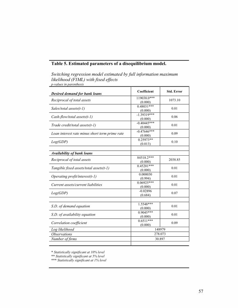
57

Table 5. Estimated parameters of a disequilibrium model.

Switching regression model estimated by full information maximum likelihood (FIML) with fixed effects p-values in parenthesis

Desired demand for bank loans

Coefficient Std. Error

Reciprocal of total assets 119038.0***

(0.000) 1073.10

Sales/total assets(t-1) 0.48031***

(0.000) 0.01

Cash-flow/total assets(t-1) -1.39319***

(0.000) 0.06

Trade credit/total assets(t-1) -0.40445***

(0.000) 0.01

Loan interest rate minus short term prime rate -0.47646***

(0.000) 0.09

Log(GDP) 0.25973**

(0.013) 0.10

Availability of bank loans

Reciprocal of total assets 84518.2***

(0.000) 2038.85

Tangible fixed assets/total assets(t-1) 0.45201***

(0.000) 0.01

Operating profit/interest(t-1) 0.000030

(0.994) 0.01

Current assets/current liabilities 0.06925***

(0.000) 0.01

Log(GDP) -0.02896

(0.684) 0.07

S.D. of demand equation 1.5548***

(0.000) 0.01

S.D. of availability equation 0.9045***

(0.000) 0.01

Correlation coefficient 0.6511***

(0.000) 0.09

Log likelihood 148979

Observations 278.073

Number of firms 30.897

* Statistically significant at 10% level ** Statistically significant at 5% level *** Statistically significant at 1% level

58

Table 6. Percentage of borrowing constrained firms

Time %

Entire period (1994-2002) 33,90

1994 34,62

1995 31,88

1996 34,22

1997 32,30

1998 34,25

1999 34,93

2000 35,16

2001 34,14

2002 33,60

Region %

ANDALUSIA 39,23

ARAGON 38,41

ASTURIAS 39,78

BALEARIC ISLANDS 28,81

CANARY ISLANDS 39,00

CANTABRIA 39,88

CASTILE LA MANCHA 39,00

CASTILE AND LEÓN 39,65

CATALONIA 32,01

COMUNIDAD VALENCIANA 29,07

EXTREMADURA 39,66

GALICIA 39,23

MADRID 31,37

MURCIA 38,23

NAVARRA 29,59

BASQUE COUNTRY 31,21

RIOJA 32,39

Sector %

MANUFACTURES OF FOOD PRODUCTS AND BEVERAGES 26,29

MANUFACTURES OF TEXTILES AND DRESSING 41,73

MANUFACTURES OF WOOD, PAPER, PRINTING AND RECORDED MEDIA PRODUCTS 39,00

MANUFACTURES OF CHEMICAL, PLASTIC, MINERAL AND METAL PRODUCTS 35,29

MANUFACTURES OF MACHINERY AND EQUIPMENT AND TRASNSPORT VEHICLES 25,22

MANUFACTURES OF FURNITURE AND RECYCLING 34,89

ELECTRICITY, GAS AND WATER SUPPLY 24,36

CONSTRUCTION 22,43

SALE, MAINTENANCE AND REPAIR OF MOTOR VEHICLES 41,75

WHOLESALE TRADE AND COMISSION TRADE 39,85

HOTELS AND RESTAURANTS 48,43

TRANSPORT SERVICES 21,31

REAL STATE ACTIVITIES 30,46

RENTING OF MACHINERY AND EQUIPMENT 32,14

COMPUTER AND RELATED ACTIVITIES 37,44

OTHER RETAIL TRADE PRODUCTS AND SERVICES 30,36

OTHER 33,33

59

Table 7. Firm financing constraints criteria. Correlations Mean values

Criterion

Trade credit/ total liabilities

(a)

Sales growth

(a)

Trade credit/ tangible assets

(a)

Loans/ tangible assets

(a)

Disequilibrium model

(constrained firms)

Trade credit/total liabilities 1.00 -0.64 0.84 -0.73 0.77

Sales growth -0.64 1.00 -0.63 0.82 -0.69

Trade credit/tangible assets 0.84 -0.63 1.00 -0.74 0.82

Loans/tangible assets -0.73 0.82 -0.74 1.00 -0.73

Disequilibrium model (constrained firms)

0.77 -0.69 0.82 -0.73 1.00

Table 8. Firm financing constraints, bank concentration and bank Lerner index Mean values

(number of firms in parenthesis)

BANK HHI (basis points) BANK LERNER INDEX (%)

Criterion

Constrained

firms

Unconstrained

firms

Constrained

firms

Unconstrained

firms

Trade credit/total liabilities (a)

0.1009 0.1040 22.62 16.96

Sales growth (a)

0.1002 0.1105 20.07 15.08

Trade credit/tangible assets (a)

0.0928 0.1108 21.73 16.11

Loans/tangible assets (a)

0.1012 0.1145 21.03 15.73

Disequilibrium model 0.1001 0.1156 20.01 16.04

(a)

: The constraint and unconstrained firms are classified considering those firms below and over the median value of

this criterion

60

Table 9. Firm financing constraints, bank concentration and market power. Regional breakdown Mean values

Bank characteristics within the region

Region

% Constrained

firms HHI

(basis points) Lerner

index (%)

Credit risk (a)

(%)

Profitability (b)

(%)

Inefficiency (c)

(%)

ANDALUCÍA 39,23 0.0926 22.05 2.26 0.76 0.68

ARAGÓN 38,41 0.0938 21.17 2.94 0.73 0.67

ASTURIAS 39,78 0.0881 22.99 2.89 0.65 0.69

BALEARES 28,81 0.1428 18.02 2.44 0.94 0.63

CANARIAS 39,00 0.0820 21.35 2.77 0.79 0.68

CANTABRIA 39,88 0.0842 22.95 2.82 0.81 0.69

CASTILLA-LEON 39,00 0.0590 22.13 2.14 0.91 0.67

CASTILLA-LA MANCHA 39,65 0.0825 20.19 2.86 0.82 0.64

CATALUNA 32,01 0.1186 16.42 2.12 0.94 0.54

COM. VALENCIANA 29,07 0.1128 17.33 2.13 0.93 0.56

EXTREMADURA 39,66 0.0908 21.96 2.63 0.81 0.62

GALICIA 39,23 0.0753 20.97 2.78 0.78 0.68

MADRID 31,37 0.1071 17.18 1.91 1.01 0.61

MURCIA 38,23 0.0761 19.36 2.44 0.72 0.68

NAVARRA 29,59 0.1263 16.05 1.58 0.94 0.57

PAISVASCO 31,21 0.1125 17.88 1.95 0.87 0.60

RIOJA 32,39 0.1401 17.93 2.17 0.99 0.59

WHOLE SAMPLE 33,90 0.1004 19.52 2.22 0.89 0.63

(a)Credit risk: Loan losses/total loans

(b) Profitability: Return on assets (ROA)

(c) Inefficiency: operating costs/gross income

61

Table 10. SMEs Financing constraints and firm, bank market and environmental conditions.

PROBIT random effects panel data results. Dependent variable = 1 if the firm is financially constrained, 0 otherwise number of points in Hermite quadrature = 20 p-values in parenthesis (I) (II)

Esitmate

Economic

significance

(marginal effecta)

Esitmate

Economic

significance

(marginal effect a)

Constant 3.4174***

(0.000) -

3.3164***

(0.000) -

Bank market power

HHI bank deposits -0.39593**

(0.010) -35.42 - -

Lerner index - - 0.02889***

(0.000) 11.3

Other bank market characteristics

Average bank size -0.40918**

(0.042) -4.12

-0.62672**

(0.041) -4.26

Bank credit risk -2.5549***

(0.000) -4.62

-2.1420***

(0.000) -5.83

Number of bank branches -0.00016***

(0.000) -0.0085

-0.000159***

(0.001) -0.0091

Bank profitability -0.281142**

(0.032) -9.67

-0.13310

(0.315) -4.01

Bank inefficiency 0.08840***

(0.005) 0.56

0.01699***

(0.000) 0.98

Firm characteristics

Firm inefficiency 0.03413***

(0.004) 2.57

0.04880**

(0.011) 6.90

Firm profitability -0.09564***

(0.000) -3.13

-0.09535***

(0.000) -4.04

Firm size 0.27370***

(0.000) 7.85

0.26986***

(0.000) 7.82

Environmental regional control variables

GDP -0.13E-05***

(0.000) -0.067

-0.15E-05***

(0.000) -0.10

Taxation 0.00040

(0.550) 0.00097

0.00047

(0.488) 0.00010

Percentage urban population 0.20669***

(0.000) 0.95

0.22799***

(0.005) 0.91

Number of bankrupticies 0.01165**

(0.014) 0.58

0.00945***

(0.000) 0.51

ρ 0.82352***

(0.000)

0.82718***

(0.000)

LR (zero slopes) 6286.44

(0.000)

5238.25

(0.000)

Log likelihood -51920.8 -44813.9

Fraction of correct predictions (%) 69.19 68.78

Observations 278.073 278.073

Number of firms 30.897 30.897

(a) marginal effects in percentage points calculated at sample means * Statistically significant at 10% level ** Statistically significant at 5% level *** Statistically significant at 1% level

62

Table 11. Cash flow-investment correlations and financing constraints. Dependent variable: Capital expenditurest/

capitalt-1 p-values in parenthesis Quartile (financing constraint variable = Trade credit(total liabilities)

Q1 Q2 Q3 Q4

Cash flowt/capitalt-1 0.3591**

(0.003)

0.5991***

(0.000)

0.9781***

(0.000)

0.9280***

(0.000)

Lagged dependent variable 0.0160

(0.670)

-0.0730**

(0.011)

0.0733**

(0.031)

0.0587

(0.412)

Lagged dependent variable2 0.0073

(0.138)

0.0018***

(0.002)

-0.10E-05

(0.357)

0.17E-05**

(0.044)

Sales 0.92E-07

(0.299)

0.11E-06

(0.214)

-0.39E-07**

(0.042)

-0.24E-07

(0.289)

Debt2 -0.19E-07**

(0.022)

-0.17E-07**

(0.023)

-0.61E-07**

(0.020)

-0.86E07**

(0.032)

Adjusted R2 0.97 0.96 0.99 0.99

Quartile (financing constraint variable = Sales growth))

Q1 Q2 Q3 Q4

Cash flowt/capitalt-1 0.96446***

(0.000)

0.95775***

(0.000)

0.48223***

(0.000)

0.58530***

(0.000)

Lagged dependent variable -0.02074

(0.757)

-0.06562

(0.755)

-0.01867

(0.366)

0.02166

(0.141)

Lagged dependent variable2 0.62E-06

(0.171)

0.55E-06

(0.212)

0.35E-06

(0.320)

0.89E-06***

(0.003)

Sales 0.72E-07

(0.323)

0.35E-08

(0.572)

-0.52E-08

(0.446)

-0.40E-07

(0.457)

Debt2 -0.18E-10

(0.298)

0.15E-09

(0.442)

-0.98E-10

(0.716)

0.39E-10***

(0.008)

Adjusted R2 0.99 0.99 0.99 0.99

Quartile (financing constraint variable = Loans/tangible assets)

Q1 Q2 Q3 Q4

Cash flowt/capitalt-1 0.91499***

(0.000)

0.85164***

(0.000)

0.55135***

(0.000)

0.58231***

(0.000)

Lagged dependent variable -0.27680***

(0.008)

0.01129

(0.350)

0.00163

(0.558)

-0.0022

(0.926)

Lagged dependent variable2 0.00012***

(0.003)

0.39E-06

(0.138)

-0.67E-05

(0.161)

0.16E-06

(0.167)

Sales 0.50E-07

(0.793)

-0.31E-07

(0.355)

0.52E-07*

(0.079)

-0.76E-08

(0.698)

Debt2 -0.20E-10

(0.654)

0.26E-10***

(0.008)

-0.39E-10

(0.648)

-0.36E-10

(0.724)

Adjusted R2 0.98 0.99 0.99 0.99

Quartile (financing constraint variable = Trade credit/tangible assets)

Q1 Q2 Q3 Q4

Cash flowt/capitalt-1 0.32780***

(0.000)

0.457754***

(0.000)

0.86695***

(0.000)

0.97559***

(0.000)

Lagged dependent variable 0.02004

(0.132)

0.04319

(0.217)

-0.18542

(0.204)

0.0483**

(0.014)

Lagged dependent variable2 0.62E-05***

(0.000)

0.38E-06

(0.103)

0.29E-05

(0.114)

0.69E-06***

(0.000)

Sales 0.12E-07

(0.838)

0.21E-07

(0.414)

0.13E-06

(0.530)

0.21E-08

(0.822)

Debt2 0.22E-10

(0.837)

0.65E-10

(0.602)

0.32E-09

(0.334)

0.31E-09

(0.859)

Adjusted R2 0.99 0.99 0.97 0.99

Quartile (financing constraint variable =Disequilibrium model)

Q1 Q2 Q3 Q4

Cash flowt/capitalt-1 0.37852***

(0.000)

0.52354***

(0.000)

0.97524***

(0.000)

0.92927***

(0.000)

Lagged dependent variable 0.12367

(0.104)

0.10587

(0.304)

0.13509*

(0.098)

0.12063

(0.149)

Lagged dependent variable2 0.73E-06***

(0.003)

0.62E-06**

(0.012)

0.68E-06***

(0.008)

0.25E-07**

(0.016)

Sales 0.13E-07

(0.658)

0.25E-07

(0.509)

0.34E-07

(0.602)

0.22E-07

(0.502)

Debt2 0.59E-10

(0.904)

0.60E-10

(0.806)

0.47E-09

(0.763)

0.28E-09

(0.397)

Adjusted R2 0.99 0.99 0.99 0.99

Observations 69.525 69.516 69.516 69.516

Number of firms 7.725 7.724 7.724 7.724

* Statistically significant at 10% level ** Statistically significant at 5% level *** Statistically significant at 1% level