Finance and Economics Discussion SeriesDivisions of Research & Statistics and Monetary Affairs

Federal Reserve Board, Washington, D.C.

Bank Market Power and the Risk Channel of Monetary Policy

Elena Afanasyeva and Jochen Guntner

2018-006

Please cite this paper as:Afanasyeva, Elena, and Jochen Guntner (2018). “Bank Market Power andthe Risk Channel of Monetary Policy,” Finance and Economics Discussion Se-ries 2018-006. Washington: Board of Governors of the Federal Reserve System,https://doi.org/10.17016/FEDS.2018.006.

NOTE: Staff working papers in the Finance and Economics Discussion Series (FEDS) are preliminarymaterials circulated to stimulate discussion and critical comment. The analysis and conclusions set forthare those of the authors and do not indicate concurrence by other members of the research staff or theBoard of Governors. References in publications to the Finance and Economics Discussion Series (other thanacknowledgement) should be cleared with the author(s) to protect the tentative character of these papers.

Bank Market Power and the Risk Channel of Monetary PolicyI

This Version: January 2018

Elena Afanasyeva∗

20th St. and Constitution Avenue, NW, 20551 Washington, DC, USA.

Email address: elena.afanasyeva@frb.gov.

Jochen Guntner∗∗

Altenbergerstrasse 69, 4040 Linz, Austria.Email address: jochen.guentner@jku.at.

Abstract

This paper investigates the risk channel of monetary policy through banks’ lending standards. We modify

the classic costly state verification (CSV) problem by introducing a risk-neutral monopolistic bank, which

maximizes profits subject to borrower participation. While the bank can diversify idiosyncratic default risk,

it bears the aggregate risk. We show that, in partial equilibrium, the bank prefers a higher leverage ratio of

borrowers, when the profitability of lending increases, e.g. after a monetary expansion. This risk channel

persists when we embed our contract in a standard New Keynesian DSGE model. Using a factor-augmented

vector autoregression (FAVAR) approach, we find that the model-implied impulse responses to a monetary

policy shock replicate their empirical counterparts.

Keywords: Costly state verification, Credit supply, Lending standards, Monetary policy, Risk channel

JEL classification: D53, E44, E52

IWe wish to thank Arpad Abraham, Tobias Adrian, Pooyan Amir Ahmadi, Martin Eichenbaum, Ester Faia, Hans Gersbach,Mark Gertler, Yuriy Gorodnichenko, Charles Kahn, Jean-Charles Rochet, Emiliano Santoro, Mirko Wiederholt, Volker Wieland,and Tao Zha as well as participants at the 2014 Cologne Workshop on Macroeconomics, the 3rd Macro Banking and FinanceWorkshop in Pavia, the XIX Vigo Workshop on Dynamic Macroeconomics, the Birkbeck Centre for Applied MacroeconomicsWorkshop, and seminar participants at CESifo, Stanford, Northwestern, Vienna and the Federal Reserve Board for helpful com-ments. Elena Afanasyeva gratefully acknowledges financial support by the German Research Foundation (DFG grant WI 2260/1-1,584 949) and the FP7 Research and Innovation Funding Program (grant FP7-SSH-2013-2). An earlier version of the paper waspreviously circulated under the title ”Lending Standards, Credit Booms, and Monetary Policy”.

∗Elena Afanasyeva is Economist at the Board of Governors of the Federal Reserve System. This paper reflects the views of theauthors and should not be interpreted as reflecting the views of the Board of Governors of the Federal Reserve System or of anyoneelse associated with the Federal Reserve System.

∗∗Jochen Guntner is Assistant Professor at the Department of Economics, Johannes Kepler University Linz.

1. Introduction

One of the narrative explanations of the credit boom preceding the recent financial crisis and the Great

Recession is that financial intermediaries took excessive risks because monetary policy rates had been “too

low for too long” (compare Taylor, 2007). On the one hand, loose monetary policy lowers the wholesale

funding costs of banks and other financial intermediaries, incentivizing higher leverage and thus risk on the

liability side of their balance sheets. On the other hand, low policy interest rates might also induce banks

to lower their lending standards, i.e. to grant more and riskier loans. While risk taking on the liability side

has received a lot of attention in the recent macroeconomic literature (see, e.g., Gertler and Karadi, 2011;

Gertler et al., 2012), much fewer studies have so far addressed the aggregate implications of a risk channel

of monetary policy on the asset side. The present paper aims at closing this gap by focusing on the ex-ante

risk attitude of banks. We develop a general equilibrium model, where the financial intermediary determines

lending standards by choosing how much to lend against a given amount of borrower collateral. Testing our

theoretical predictions empirically, we find robust evidence for an asset-side risk channel of monetary policy

in the U.S. banking sector, consistent with the model.

In this paper, we provide a microeconomic foundation for banks’ decision to lower their “lending stan-

dards” in response to a monetary expansion. To this end, we reformulate the costly state verification (CSV)

contract in Townsend (1979) and Gale and Hellwig (1985) in order to allow for a nontrivial role of financial

intermediaries. The CSV contract provides a natural starting point, given that its parties determine both the

quantity of credit (via the amount lent) and the quality of credit (via the borrower’s ex-ante implied default

risk). However, in conventional implementations of the contract in models of the financial accelerator, such

as Bernanke et al. (1999), financial intermediaries are passive and do not bear any risk.

We depart from these assumptions and introduce a monopolistic bank that chooses its lending standards.

The resulting contract is incentive-compatible, robust to ex-post renegotiations, and resembles a standard

debt contract (compare Gale and Hellwig, 1985). It also implies a unique partial equilibrium solution and the

well-known positive relationship between the expected external finance premium (EFP) and the borrower’s

leverage ratio. Following an exogenous increase in the expected EFP, e.g. due to a monetary expansion, the

monopolistic bank finds it profitable to lend more against a given amount of borrower collateral. The reason

is that it benefits from the increase in borrower leverage through a larger share in total profits, while it can

price in the higher default probability of the borrower through the rate of return on non-defaulting loans,

2

thus increasing its net interest margin.

In order to quantify the effects of our partial equilibrium mechanism in response to a monetary expansion

and over the business cycle, we embed our modified and the classic version of the optimal debt contract in

an otherwise standard New Keynesian dynamic stochastic general equilibrium (DSGE) model. In contrast

to Bernanke et al. (1999) and most of the existing literature, our model implies an increase in bank lending

relative to borrower collateral and thus a higher leverage ratio of borrowers in response to an expansionary

monetary policy shock. Over the business cycle, both models can replicate the dynamic cross-correlations of

key variables with output qualitatively and quantitatively, while our model also replicates the unconditional

moments of bank-related balance sheet variables that are either missing or constant in standard models of

the financial accelerator.

Prior research based on microeconomic bank-level data (Jimenez et al., 2014; Ioannidou et al., 2015)

has shown that lower overnight interest rates might induce banks to commit larger loan volumes with fewer

collateral requirement to ex-ante riskier firms. Similarly, Paligorova and Santos (2017) use bank-loan data

and find compelling evidence in favor of the risk-taking channel of monetary policy in the U.S. For macroe-

conomic time series, the results in the literature are rather ambiguous (see, e.g., Buch et al., 2014). The use

of aggregated data in this context is complicated by the limited availability of suitable measures of banks’

risk appetite and a comparatively short sample period. On the one hand, econometric models with an exces-

sive number of parameters are thus prone to overfitting. On the other hand, small-scale VAR models might

contain insufficient information to identify the structural shocks of interest (compare Forni and Gambetti,

2014). To address these issues, we adopt the factor-augmented vector autoregression (FAVAR) approach

proposed by Bernanke et al. (2005), which allows us to parsimoniously extract information from a large

set of macroeconomic time series, thereby mitigating both the concern of overfitting and the concern of

informational sufficiency.

To capture the credit-risk attitude of banks, we use the quantified qualitative measures from the Federal

Reserve’s Senior Loan Officer Opinion Survey on Bank Lending Practices (SLOOS)1, which reflect changes

in lending standards of large domestic as well as U.S. branches and agencies of foreign banks at a quarterly

frequency, starting in 1991Q1. In contrast to the prior empirical literature, we consider 19 different measures

of lending standards, such as the net percentage of banks increasing collateral requirements or tightening

1These data are publicly available at https://www.federalreserve.gov/data/sloos/sloos.htm.

3

loan covenants for various categories of loans, borrowers and banks, in order to capture the comovement

in the underlying time series. Based on Bernanke et al.’s (2005) one-step Bayesian estimation approach by

Gibbs sampling with recursive identification of monetary policy shocks, we find that all 19 SLOOS measures

of lending standards decrease in response to a monetary expansion. This loosening of lending standards is

accompanied by an increase in loan riskiness2, the net interest margin and bank profits from the so-called

Call Reports that is qualitatively and quantitatively in line with our theoretical predictions.

Our empirical findings are qualitatively robust to variations in the FAVAR specification and alternative

identification strategies. In light of recent evidence that U.S. monetary policy became more forward-looking

during our sample period, we include variables from the Fed’s Greenbook in the FAVAR observation equa-

tion. Among further robustness checks, we adopt the high-frequency identification approach in Barakchian

and Crowe (2013), which does not rely on a VAR specification.

We finally find that our results carry over to alternative measures of financial intermediaries’ risk ap-

petite. In particular, we show that Bassett et al.’s (2014) measure of the supply component of bank lending

standards decreases, while the net percentage of domestic banks easing lending standards due to higher risk

tolerance increases in response to a monetary expansion. Moreover, two market-based measures of lend-

ing standards – Gilchrist and Zakrajsek’s (2012) “excess bond premium” and the Chicago Fed’s National

Financial Conditions credit subindex – decrease significantly after an expansionary monetary policy shock.

The remainder of our paper is organized as follows. Section 2 derives the optimal financial contract and

discusses the risk channel in partial equilibrium. In Section 3, we embed this contract in a quantitative New

Keynesian DSGE model. Section 4 sketches our econometric approach and presents new empirical evidence

of an asset-side risk channel of monetary policy in the U.S. banking sector. Section 5 concludes.

2. The Optimal Debt Contract in Partial Equilibrium

In this section, we show that it can be optimal for a lender to increase the amount of credit per unit of

borrower collateral in response to expansionary monetary policy, even if this raises the default probability of

a given borrower and the default rate across borrowers. In other words, the lender lowers its credit standards.

To this end, we draw on a problem of the type analyzed in Townsend (1979) and Gale and Hellwig (1985),

and embedded in a New Keynesian DSGE model by Bernanke et al. (1999). The CSV contract accounts for

2Loan riskiness is measured as an average risk score from the Terms of Business Lending Survey of the Federal Reserve.

4

both dimensions of a credit expansion: (i) the quantity of credit, i.e. the amount lent, and (ii) the quality of

credit, i.e. the expected default threshold of the borrower that a bank is willing to tolerate. It provides thus a

micro-foundation for banks’ optimal decision on lending standards during a credit expansion.

In contrast to Bernanke et al. (1999) and most recent contributions, we formulate the optimal financial

contract from the lender’s perspective.3 In particular, we assume that a risk-neutral bank decides how much

to lend against a given amount of borrower collateral. Accordingly, the bank determines the entrepreneur’s

total capital expenditure and expected default threshold. Note that introducing an active financial interme-

diary is a prerequisite for analyzing the effect of monetary policy on bank lending standards. In our model,

the latter are endogenously determined through the bank’s constrained profit-maximization problem.

We further assume that market power in the credit market is in the hands of the bank, which makes a

“take-it-or-leave-it” loan offer to borrowers, similar to that in Valencia (2014). In order for a firm to accept

this offer, it must be at least as well off with as without the loan. While representing one of many conceivable

profit-sharing agreements, this can be motivated by the prevalence of relationship lending between banks

and small or medium-sized enterprises.4 In what follows, we specify the details of the optimal loan contract

in partial equilibrium. Assuming that each entrepreneur borrows from at most one bank, the latter can

enter a contract with one entrepreneur independently of its relations with others, and we can consider a

representative bank-entrepreneur pairing (compare Gale and Hellwig, 1985).

2.1. The Contracting Problem

Suppose that, at time t, entrepreneur i purchases capital QtKit for use at t + 1, where Ki

t is the quantity

of capital purchased and Qt is the price of one unit of capital in period t. The gross return per unit of capital

expenditure by entrepreneur i, ωit+1Rk

t+1, depends on the ex-post aggregate return on capital, Rkt+1, and an

idiosyncratic component, ωit+1. Following Bernanke et al. (1999), the random variable ωi

t+1 ∈ [0,∞) is i.i.d.

across entrepreneurs i and time t, with a continuous and differentiable cumulative distribution function F (ω)

and an expected value of unity.

3Recall that, in Bernanke et al. (1999), there is no active role for the so-called “financial intermediary”, which merely diversifiesaway the idiosyncratic productivity risks of entrepreneurs and institutionalizes the participation constraint of a risk-averse depositor,along which the firm moves when making its optimal capital and borrowing decision.

4For example, Petersen and Rajan (1995) use a simple dynamic setting to show that the value of lending relationships decreasesin the degree of competition in credit markets. The reason is that a monopolist lender can postpone interest payments in order toextract future rents from the borrowing firm, effectively “subsidizing the firm when young or distressed and extracting rents later”(Petersen and Rajan, 1995, p.408). A similar argument applies for the monopolist bank in our model, which can fully diversify theidiosyncratic productivity risks by lending to the entire cross section of firms.

5

Entrepreneur i finances capital purchases at the end of period t using accumulated net worth, Nit , as well

as the borrowed amount Bit, so that the entrepreneur’s balance sheet is given by

QtKit = Ni

t + Bit. (1)

Abstracting from alternative investment opportunities of entrepreneurs, the maximum equity participa-

tion (MEP) condition in Gale and Hellwig (1985) is trivially satisfied.5 As in Valencia (2014), entrepreneur

i borrows the amount Bit from a monopolistic bank, that is endowed with end-of-period-t net worth or bank

capital Nbt and raises deposits Dt from households. Defining aggregate lending to borrowers as Bt ≡

∫ 10 Bi

tdi,

the bank’s aggregate balance sheet identity in period t is given by

Bt ≡ Nbt + Dt. (2)

The need for borrower collateral arises from the presence of a state-verification cost paid by the lender

in order to observe entrepreneur i’s realization of ωit+1, which is private information. We assume that this

cost corresponds to a fixed proportion µ ∈ (0, 1] of the entrepreneur’s total return on capital in period t + 1,

ωit+1Rk

t+1QtKit , so that initially uninformed agents may become informed by paying a fee which depends on

the invested amount and the state (compare Townsend, 1979).

Both the borrower and the lender are risk-neutral and care about expected returns only, whereas deposi-

tors are risk-averse. Accordingly, the bank promises to pay the risk-free gross rate of return Rnt on deposits

in each aggregate state of the world, as characterized by the realization of Rkt+1.

Let Zit denote the gross non-default rate of return on the period-t loan to entrepreneur i. Given Rk

t+1,

QtKit , and Ni

t , the financial contract defines a relationship between Zit and an ex-post cutoff value

ωit+1 ≡

Zit B

it

Rkt+1QtKi

t, (3)

such that the borrower pays the lender the fixed amount ωit+1Rk

t+1QtKit and keeps the residual

(ωi

t+1 − ωit+1

)·

Rkt+1QtKi

t if ωit+1 ≥ ω

it+1. If ωi

t+1 < ωit+1, the lender monitors the borrower, incurs the CSV cost, and extracts

the remainder (1 − µ)ωit+1Rk

t+1QtKit , while the entrepreneur defaults and receives nothing.

In contrast to Bernanke et al. (1999), we assume that the lender determines the amount of credit to

entrepreneur i, Bit, for a given amount of borrower collateral, Ni

t . Yet, the entrepreneur will only accept the

5Proposition 2 in Gale and Hellwig (1985) states that any optimal contract is weakly dominated by a contract with MEP, wherethe firm puts all of its own liquid assets – here N i

t – on the table.

6

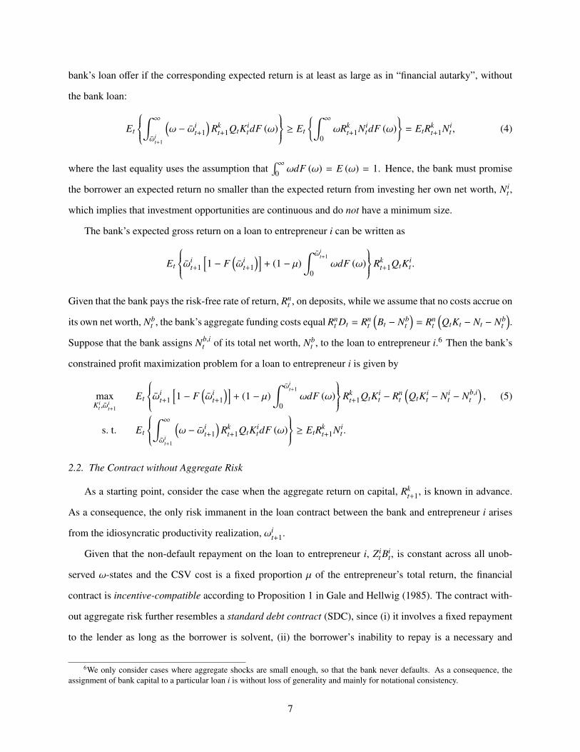
bank’s loan offer if the corresponding expected return is at least as large as in “financial autarky”, without

the bank loan:

Et

∫ ∞

ωit+1

(ω − ωi

t+1

)Rk

t+1QtKitdF (ω)

≥ Et

∫ ∞

0ωRk

t+1NitdF (ω)

= EtRk

t+1Nit , (4)

where the last equality uses the assumption that∫ ∞

0 ωdF (ω) = E (ω) = 1. Hence, the bank must promise

the borrower an expected return no smaller than the expected return from investing her own net worth, Nit ,

which implies that investment opportunities are continuous and do not have a minimum size.

The bank’s expected gross return on a loan to entrepreneur i can be written as

Et

ωit+1

[1 − F

(ωi

t+1

)]+ (1 − µ)

∫ ωit+1

0ωdF (ω)

Rkt+1QtKi

t .

Given that the bank pays the risk-free rate of return, Rnt , on deposits, while we assume that no costs accrue on

its own net worth, Nbt , the bank’s aggregate funding costs equal Rn

t Dt = Rnt

(Bt − Nb

t

)= Rn

t

(QtKt − Nt − Nb

t

).

Suppose that the bank assigns Nb,it of its total net worth, Nb

t , to the loan to entrepreneur i.6 Then the bank’s

constrained profit maximization problem for a loan to entrepreneur i is given by

maxKi

t ,ωit+1

Et

ωit+1

[1 − F

(ωi

t+1

)]+ (1 − µ)

∫ ωit+1

0ωdF (ω)

Rkt+1QtKi

t − Rnt

(QtKi

t − Nit − Nb,i

t

), (5)

s. t. Et

∫ ∞

ωit+1

(ω − ωi

t+1

)Rk

t+1QtKitdF (ω)

≥ EtRkt+1Ni

t .

2.2. The Contract without Aggregate Risk

As a starting point, consider the case when the aggregate return on capital, Rkt+1, is known in advance.

As a consequence, the only risk immanent in the loan contract between the bank and entrepreneur i arises

from the idiosyncratic productivity realization, ωit+1.

Given that the non-default repayment on the loan to entrepreneur i, Zit B

it, is constant across all unob-

served ω-states and the CSV cost is a fixed proportion µ of the entrepreneur’s total return, the financial

contract is incentive-compatible according to Proposition 1 in Gale and Hellwig (1985). The contract with-

out aggregate risk further resembles a standard debt contract (SDC), since (i) it involves a fixed repayment

to the lender as long as the borrower is solvent, (ii) the borrower’s inability to repay is a necessary and

6We only consider cases where aggregate shocks are small enough, so that the bank never defaults. As a consequence, theassignment of bank capital to a particular loan i is without loss of generality and mainly for notational consistency.

7

sufficient condition for bankruptcy, and (iii) if the borrower defaults, the bank recovers as much as it can.7

Hence, the optimal contract between the bank and each entrepreneur is a SDC with MEP, as in Bernanke

et al. (1999). Moreover, the optimal contract is robust to ex-post renegotiations, if µ represents a pure ver-

ification cost rather than a bankruptcy cost. In the latter case, it would be optimal to renegotiate the terms

of the loan ex post in order to avoid default, whereas, in the former case, incentive compatibility requires

monitoring the borrower whenever he or she cannot repay.8

For notational convenience, let

Γ(ωi

t

)≡ ωi

t

[1 − F

(ωi

t

)]+

∫ ωit

0ωdF (ω) and µG

(ωi

t

)= µ

∫ ωit

0ωdF (ω)

denote the expected share of total profits and the expected CSV costs accruing to the lender in period t,

where 0 < Γ(ωi

t

)< 1 by definition, and note that

Γ′(ωi

t

)= 1 − F

(ωi

t

)> 0, Γ′′

(ωi

t

)= − f

(ωi

t

)< 0, µG′

(ωi

t

)≡ µωi

t f(ωi

t

)> 0.

We can then write the expected share of total profits net of monitoring costs received by the lender and the

expected share of total profits going to the borrower as Γ(ωi

t

)− µG

(ωi

t

)and 1 − Γ

(ωi

t

), respectively.

Defining the expected external finance premium (EFP), st ≡ Rkt+1/R

nt , the entrepreneur’s capital/net

worth ratio, kit ≡ QtKi

t/Nit , as well as ni

t ≡ Nb,it /Ni

t and using the above notation, the bank’s constrained profit

maximization problem in (5) can equivalently be written as

maxki

t ,ωit+1

[Γ(ωi

t+1) − µG(ωit+1)

]stki

t − (kit − 1 − ni

t) s. t.[1 − Γ(ωi

t+1)]

stkit = st, (6)

where we have omitted the expectations operator, since Rkt+1 and thus st are assumed to be known in advance.

The corresponding first-order conditions with respect to kit, ω

it+1, and the Lagrange multiplier λi

t are

kit :

[Γ(ωi

t+1) − µG(ωit+1)

]st − 1 + λi

t

[1 − Γ(ωi

t+1)]

st = 0,

ωit+1 :

[Γ′(ωi

t+1) − µG′(ωit+1)

]stki

t − λitΓ′(ωi

t+1)stkit = 0,

λit :

[1 − Γ(ωi

t+1)]

stkit − st = 0.

7Proposition 3 in Gale and Hellwig (1985) states that any contract is weakly dominated by a SDC with the above three features.8The central assumption is that the bank incurs the CSV cost in order to verify the entrepreneur’s idiosyncratic realization of ω

before agreeing to renegotiate, because the borrower cannot truthfully report default without the risk of being monitored (compareCovas and Den Haan, 2012).

8

Figure 1: Illustration of the Optimal CSV Contract without Aggregate Risk and the Effects of Expansionary Monetary Policy.

0.1 0.2 0.3 0.4 0.5 0.6 0.7 0.8 0.9

1

1.5

2

2.5

3

3.5

4

4.5

5

5.5

ω

k(ω

)

Iso profit curves (lender)Participation constraint (borrower)

0.1 0.2 0.3 0.4 0.5 0.6 0.7 0.8 0.9

1

1.5

2

2.5

3

3.5

4

4.5

5

5.5

6

ω

k(ω

)

Old iso profit curves (lender)New iso profit curves (lender)Participation constraint (borrower)

0.3 0.35 0.4 0.45 0.5 0.55 0.6 0.651.4

1.6

1.8

2

2.2

2.4

2.6

2.8

ω∗old

ω ω∗new

k∗ ol

d

k(

ω)

k

∗ new

Old tangential iso profit curve (lender)New tangential iso profit curve (lender)Participation constraint (borrower)

9

Proposition 1. The optimal contract implies a positive relationship, kit = ψ(st) with ψ′(st) > 0, between the

expected EFP, st ≡ Rkt+1/R

nt , and the optimal capital/net worth ratio, ki

t ≡ QtKit/N

it .

Proof. See Appendix A.1.

Accordingly, an exogenous increase in the expected EFP, for example due to a reduction in the risk-free

rate, Rnt , induces the bank to lend more against a given amount of borrower net worth and thus collateral.

2.3. The Risk Channel

The mechanism driving our partial equilibrium result is illustrated in Figure 1, where time subscripts and

index superscripts are suppressed for notational convenience. Note that the lender’s iso-profit curves (IPCs)

and the borrower’s participation constraint (PC) can be plotted in (k, ω)-space and that the constrained profit

maximum of the bank is determined by the tangential point between the PC and the (lowest) IPC.9 The

corresponding expressions for the borrower’s PC and the lender’s IPC are

kPC ≥1

1 − Γ(ω)(7)

andkIPC =

πb − 1 − n[Γ(ω) − µG(ω)

]s − 1

, (8)

where πb denotes an arbitrary level of bank profits.

From (7), the PC is not affected by the EFP, s. In the absence of aggregate risk, the borrower’s expected

share of total profits, 1−Γ (ω), must be no smaller than her “skin in the game”, 1/k ≡ N/QK. For any given

ω and thus an expected share of total profits, the borrower’s PC determines a minimum value of the lender’s

“skin in the game”, k, below which the entrepreneur does not accept the offered loan contract. The bank’s

IPC in (8) accounts for expected monitoring and funding costs. By choosing the tangential point between

the borrower’s PC and its lowest IPC in (k, ω)-space, the bank minimizes its “skin in the game” for a given

expected share of total profits, Γ (ω). Note that, for QK = N, the borrower is fully self-financed, never

defaults (ω = 0), and retains all the profits (1 − Γ (0) = 1).

The first panel of Figure 1 illustrates the tangential point between the borrower’s PC and the lender’s

IPC for the calibration in Bernanke et al. (1999). Now consider the effects of a monetary expansion, i.e.

9Online Appendix A.1 proves that the optimal contract yields a unique interior solution.

10

a decrease in Rn and thus an increase in s ≡ Rk/Rn, where Rk is known in advance. While the borrower’s

PC remains unaffected, the lender’s IPCs are tilted upwards, as shown in the second panel. Although the

borrower would accept any point above its PC on the new IPC, this is no longer optimal from the lender’s

perspective. The bank can move to a lower IPC and thus to a higher level of profits, as indicated in the third

panel. In doing so, however, it must satisfy the borrower’s PC, as in the new optimal contract (k∗new, ω∗new),

where both the bank’s expected profit share, Γ(ω), and its “skin in the game”, k, have increased.

The previous discussion illustrates a crucial feature of the optimal debt contract. For a profit-maximizing

bank, it is optimal to respond to an increase in the EFP (e.g. due to a monetary expansion) by lending more

against a given amount of collateral, thus increasing the entrepreneur’s leverage ratio. In partial equilibrium,

a similar qualitative result arises from the optimal debt contract in Bernanke et al. (1999), yet for a different

reason. In particular, financial intermediaries make zero profits and the lender’s PC just equates the expected

return on the loan net of monitoring costs to the risk-free rate. A monetary expansion loosens the PC and

induces the entrepreneur to raise more external funds against a given amount of collateral, while the expected

return to the lender decreases. The expansion of credit is therefore driven by a shift in demand due to the

increased creditworthiness of borrowers.

In contrast, the increase in the borrower’s leverage ratio in Figure 1 represents the optimal response of

the bank. In our model, a monetary expansion lowers the interest rate on deposits and thus the funding cost

of the lender in (5), while it does not affect the borrower’s PC in (4). Ceteris paribus, the profitability of

the marginal loan increases, whereas the demand for credit is unchanged. Since entrepreneurs’ net worth

is predetermined, the increase in lending leads to an increase in borrower leverage. From (3), the higher

leverage ratio implies a higher default threshold, ω, and a higher default probability of the loan. This

corresponds to the risk-taking channel of monetary policy described, for example, in Adrian and Shin (2011)

and Borio and Zhu (2012). By affecting the rates of return on both sides of the bank’s balance sheet, a

monetary expansion raises the profitability of financial intermediaries, thus shifting the supply of credit.

While moving along the borrower’s PC, the bank must compensate the entrepreneur for a lower share of

total profits by increasing its own “skin in the game”.

2.4. The Contract with Aggregate Risk

In the dynamic model, the aggregate return on capital is ex ante uncertain. As a consequence, the default

threshold characterizing a loan contract between the bank and entrepreneur i, ωit+1, generally depends on

11

the ex-post realization of Rkt+1. Bernanke et al. (1999) circumvent this complication by presuming that,

given the risk aversion of depositors, the lender’s participation constraint must be satisfied ex post and the

entrepreneur bears any aggregate risk. Similarly, we assume that the borrower’s PC must be satisfied ex post

and that the bank absorbs any aggregate risk. This assumption is only viable, if the bank’s capital buffer, Nbt ,

is sufficient to shield depositors from any fluctuations in Rkt+1, so that the bank never defaults.10

In order to understand the implications of our assumption, recall the PC in equation (7). Given that the

borrower’s capital expenditure, QtKit , and net worth, Ni

t , are predetermined in period t + 1, the ex-post share

of total profits, 1 − Γ(ωi

t+1

), and the corresponding default threshold, ωi

t+1, can not be made contingent on

the aggregate state of the economy. From the definition of the cutoff in (3), the non-default rate of return,

Zit , must then be state-contingent in order to offset unexpected realizations of Rk

t+1.

In contrast to Bernanke et al. (1999), where both ωit+1 and Zi

t are state-contingent and countercyclical (in

the sense that a higher than expected realization of Rkt+1 lowers the default threshold and the non-default rate

of return required by the lender), here ωit+1 is predetermined and acyclical, while Zi

t is procyclical. Higher

than expected realizations of Rkt+1 raise Zi

t , whereas the borrower’s and the lender’s expected profit shares

are determined by their “skin in the game”, i.e. by the relative shares of Nit and Bi

t in QtKit . Although neither

of the ex-post versions seems fully consistent with the common perception that the non-default rate of return

on bank credit is predetermined and thus acyclical, the procyclicality of Zit in our contract can be interpreted

as the bank having a stake in the firm in terms of either equity or a long-term lending relationship. Hence, it

is in the bank’s interest that borrowers default only due to idiosyncratic risk, which can be diversified away,

rather than due to aggregate risk. While a formal proof is beyond the scope of the current paper, Appendix

A.3 provides a simple heuristical argument for the optimality of this risk-sharing agreement.

The ex-post version of our financial contract is incentive-compatible and resembles a standard debt

contract, if and only if Rkt+1 is observed by both parties without incurring a cost (compare Gale and Hellwig,

1985).11 Otherwise, the non-default rate of return on the loan, Zit , can not be made contingent on the state

of the economy, whereas entrepreneurs generally have no incentive to misreport a true observed state.

10In other words, we assume that the fluctuations in the bank’s net return on lending,∫ 1

0

[Γ(ωi

t+1

)− µG

(ωi

t+1

)]Rk

t+1QtKit di, are

small enough to be absorbed without the bank defaulting.11One could argue that, by holding a perfectly diversified loan portfolio, the bank can deduce the ex-post realization of Rk

t+1,unless entrepreneurs misreport their returns in an unobserved state in a systematic way across i. However, we already know thatentrepreneurs have no incentive to lie, if Zi

t is independent of ωit+1. Note that a similar argument must implicitly hold in Bernanke

et al. (1999) for optimality.

12

Proposition 2. Even in the case with aggregate risk, the optimal contract between the bank and entrepreneur

i implies a positive relationship, kit = ψ (st) with ψ′(st) > 0, between the expected EFP, st ≡ Et

Rk

t+1

/Rn

t ,

and the optimal capital/net worth ratio, kit ≡ QtKi

t/Nit .

Proof. See Appendix A.2.

3. The General Equilibrium Model

While the previous section illustrates that a monetary expansion might induce a profit-maximizing bank

to lower its lending standards, the partial equilibrium analysis is confined to variables specified in the con-

tract. In what follows, we embed both our optimal debt contract and the contract in Bernanke et al. (1999)

in an otherwise standard New Keynesian DSGE model in order to be able to quantify their implications for

a variety of macroeconomic variables, in response to a monetary policy shock and over the business cycle.

The general equilibrium model comprises eight types of economic agents: A representative household,

perfectly competitive capital goods and intermediate goods producers, a continuum of monopolistically

competitive labor unions and retailers, respectively, a monetary authority, a continuum of entrepreneurs, and

a monopolistic bank. Since we borrow the former six from the existing literature, only entrepreneurs and

the bank are discussed here in detail.

3.1. The Model Environment

The representative household supplies homogeneous labor to monopolistically competitive labor unions,

consumes, and saves in terms of risk-free bank deposits. The representative capital goods producer buys the

non-depreciated capital stock from entrepreneurs, makes an investment decision subject to adjustment costs,

and sells the new capital stock to entrepreneurs within the same period without incurring any capital gains

or losses. The representative intermediate goods producer rents capital from entrepreneurs, hires labor from

labor unions, and sells intermediate output to retailers in a competitive wholesale market. Retailers (unions)

diversify the homogeneous intermediate good (labor input of households) without incurring any costs and

are thus able to set the price on final output (wage) above their marginal cost, i.e. the price of the intermediate

good.12 Monetary policy follows a standard Taylor (1993) rule. Since the optimization problems of these

12Monopolistically competitive labor unions and retailers are introduced in order to allow for nominal wage and price rigiditieswithout unnecessarily complicating the production and investment decisions of firms (compare Bernanke et al., 1999).

13

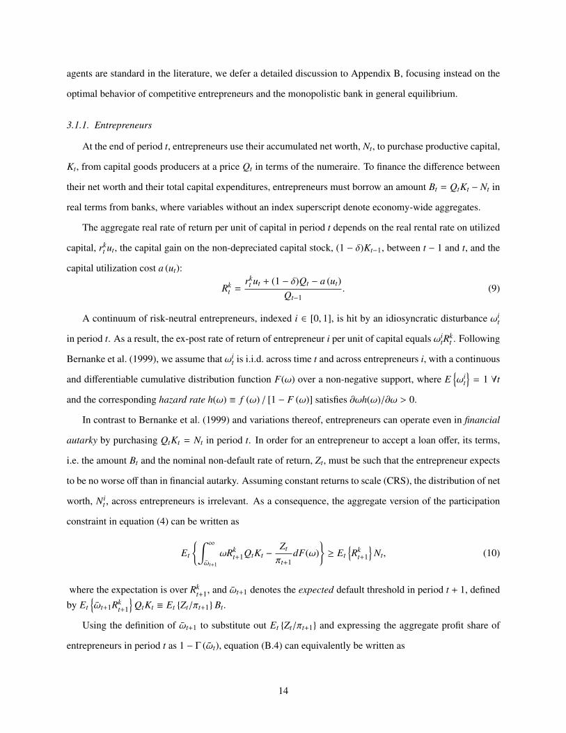
agents are standard in the literature, we defer a detailed discussion to Appendix B, focusing instead on the

optimal behavior of competitive entrepreneurs and the monopolistic bank in general equilibrium.

3.1.1. Entrepreneurs

At the end of period t, entrepreneurs use their accumulated net worth, Nt, to purchase productive capital,

Kt, from capital goods producers at a price Qt in terms of the numeraire. To finance the difference between

their net worth and their total capital expenditures, entrepreneurs must borrow an amount Bt = QtKt − Nt in

real terms from banks, where variables without an index superscript denote economy-wide aggregates.

The aggregate real rate of return per unit of capital in period t depends on the real rental rate on utilized

capital, rkt ut, the capital gain on the non-depreciated capital stock, (1 − δ)Kt−1, between t − 1 and t, and the

capital utilization cost a (ut):

Rkt =

rkt ut + (1 − δ)Qt − a (ut)

Qt−1. (9)

A continuum of risk-neutral entrepreneurs, indexed i ∈ [0, 1], is hit by an idiosyncratic disturbance ωit

in period t. As a result, the ex-post rate of return of entrepreneur i per unit of capital equals ωitR

kt . Following

Bernanke et al. (1999), we assume that ωit is i.i.d. across time t and across entrepreneurs i, with a continuous

and differentiable cumulative distribution function F(ω) over a non-negative support, where Eωi

t

= 1 ∀t

and the corresponding hazard rate h(ω) ≡ f (ω) / [1 − F (ω)] satisfies ∂ωh(ω)/∂ω > 0.

In contrast to Bernanke et al. (1999) and variations thereof, entrepreneurs can operate even in financial

autarky by purchasing QtKt = Nt in period t. In order for an entrepreneur to accept a loan offer, its terms,

i.e. the amount Bt and the nominal non-default rate of return, Zt, must be such that the entrepreneur expects

to be no worse off than in financial autarky. Assuming constant returns to scale (CRS), the distribution of net

worth, Nit , across entrepreneurs is irrelevant. As a consequence, the aggregate version of the participation

constraint in equation (4) can be written as

Et

∫ ∞

ωt+1

ωRkt+1QtKt −

Zt

πt+1dF(ω)

≥ Et

Rk

t+1

Nt, (10)

where the expectation is over Rkt+1, and ωt+1 denotes the expected default threshold in period t + 1, defined

by Etωt+1Rk

t+1

QtKt ≡ Et Zt/πt+1 Bt.

Using the definition of ωt+1 to substitute out Et Zt/πt+1 and expressing the aggregate profit share of

entrepreneurs in period t as 1 − Γ (ωt), equation (B.4) can equivalently be written as

14

Et[1 − Γ (ωt+1)] Rk

t+1

QtKt ≥ Et

Rk

t+1

Nt. (11)

Note that the ex-post realized value of Γ (ωt+1) generally depends on the realization of Rkt+1 through ωt+1.

Similar to Bernanke et al. (1999), we assume that this constraint must be satisfied ex post. Implicit in this

is the assumption that Rkt+1 is observed by both parties without incurring a cost, and that the non-default

repayment, Zt, can thus be made contingent on the aggregate state of the economy.

In order to avoid that entrepreneurial net worth grows without bound, we assume that an exogenous

fraction (1 − γe) of the entrepreneurs’ share of total realized profits is consumed each period.13 As a result,

entrepreneurial net worth at the end of period t evolves according to

Nt = γe [1 − Γ(ωt)] Rkt Qt−1Kt−1. (12)

To sum up, the entrepreneurs’ equilibrium conditions comprise the real rate of return per unit of capital

in (B.3), the ex-post participation constraint in (B.5), the evolution of entrepreneurial net worth in (B.6),

and the real amount borrowed, Bt = QtKt − Nt. Moreover, the definition of the expected default threshold,

Etωt+1, determines the expected non-default repayment per unit borrowed by the entrepreneurs, Et Zt/πt+1.

3.1.2. The Bank

For tractability, we assume a single monopolistic financial intermediary, which collects deposits from

households and provides loans to entrepreneurs. In period t, this bank is endowed with net worth or bank

capital Nbt . Abstracting from bank reserves or other types of bank assets, its balance sheet identity in real

terms is given by equation (2). The CSV problem in Townsend (1979) implies that, if entrepreneur i defaults

due to ωitR

kt Qt−1Ki

t−1 <(Zi

t−1/πt)

Bit−1, the bank incurs a proportional cost µωi

tRkt Qt−1Ki

t−1 and recovers the

remaining return on capital, (1 − µ)ωitR

kt Qt−1Ki

t−1.

In period t, the risk-neutral bank observes entrepreneurs’ net worth, Nit , and makes a take-it-or-leave-it

offer to each entrepreneur i. As a consequence, it holds a perfectly diversified loan portfolio between period

t and period t +1. Although the bank can thus diversify away any idiosyncratic risk arising from the possible

default of entrepreneur i, it is subject to aggregate risk through fluctuations in the ex-post rate of return on

capital, Rkt+1, and the aggregate default threshold, ωt+1. In order to be able to pay the risk-free nominal

13In the literature, it is common to assume that an exogenous fraction of entrepreneurs “dies” each period and consumes its networth upon exit. The dynamic implications of either assumption are identical.

15

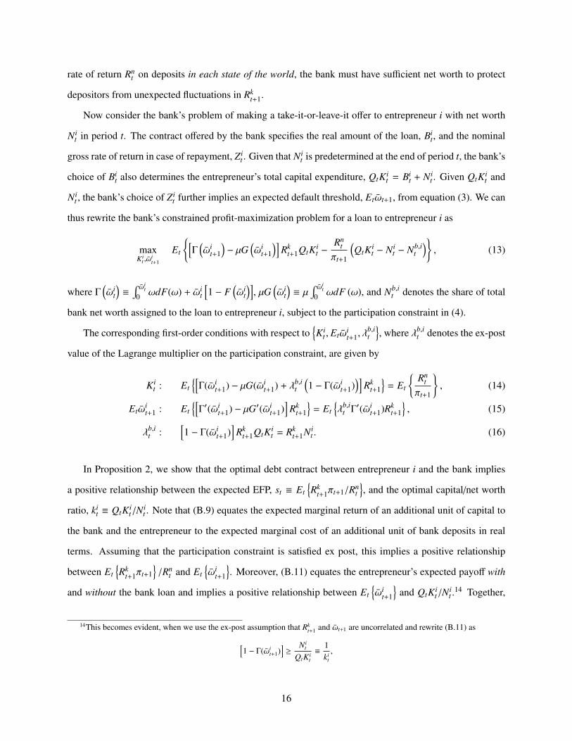
rate of return Rnt on deposits in each state of the world, the bank must have sufficient net worth to protect

depositors from unexpected fluctuations in Rkt+1.

Now consider the bank’s problem of making a take-it-or-leave-it offer to entrepreneur i with net worth

Nit in period t. The contract offered by the bank specifies the real amount of the loan, Bi

t, and the nominal

gross rate of return in case of repayment, Zit . Given that Ni

t is predetermined at the end of period t, the bank’s

choice of Bit also determines the entrepreneur’s total capital expenditure, QtKi

t = Bit + Ni

t . Given QtKit and

Nit , the bank’s choice of Zi

t further implies an expected default threshold, Etωt+1, from equation (3). We can

thus rewrite the bank’s constrained profit-maximization problem for a loan to entrepreneur i as

maxKi

t ,ωit+1

Et

[Γ(ωi

t+1

)− µG

(ωi

t+1

)]Rk

t+1QtKit −

Rnt

πt+1

(QtKi

t − Nit − Nb,i

t

), (13)

where Γ(ωi

t

)≡

∫ ωit

0 ωdF(ω) + ωit

[1 − F

(ωi

t

)], µG

(ωi

t

)≡ µ

∫ ωit

0 ωdF (ω), and Nb,it denotes the share of total

bank net worth assigned to the loan to entrepreneur i, subject to the participation constraint in (4).

The corresponding first-order conditions with respect toKi

t , Etωit+1, λ

b,it

, where λb,i

t denotes the ex-post

value of the Lagrange multiplier on the participation constraint, are given by

Kit : Et

[Γ(ωi

t+1) − µG(ωit+1) + λb,i

t

(1 − Γ(ωi

t+1))]

Rkt+1

= Et

Rn

t

πt+1

, (14)

Etωit+1 : Et

[Γ′(ωi

t+1) − µG′(ωit+1)

]Rk

t+1

= Et

λb,i

t Γ′(ωit+1)Rk

t+1

, (15)

λb,it :

[1 − Γ(ωi

t+1)]

Rkt+1QtKi

t = Rkt+1Ni

t . (16)

In Proposition 2, we show that the optimal debt contract between entrepreneur i and the bank implies

a positive relationship between the expected EFP, st ≡ EtRk

t+1πt+1/Rnt

, and the optimal capital/net worth

ratio, kit ≡ QtKi

t/Nit . Note that (B.9) equates the expected marginal return of an additional unit of capital to

the bank and the entrepreneur to the expected marginal cost of an additional unit of bank deposits in real

terms. Assuming that the participation constraint is satisfied ex post, this implies a positive relationship

between EtRk

t+1πt+1/Rn

t and Etωi

t+1

. Moreover, (B.11) equates the entrepreneur’s expected payoff with

and without the bank loan and implies a positive relationship between Etωi

t+1

and QtKi

t/Nit .

14 Together,

14This becomes evident, when we use the ex-post assumption that Rkt+1 and ωt+1 are uncorrelated and rewrite (B.11) as

[1 − Γ(ωi

t+1)]≥

N it

QtKit≡

1ki

t,

16

these two conditions determine the positive ex-ante relationship between the expected EFP in period t + 1

and the leverage ratio chosen by the bank in period t, while the first-order condition with respect to Etωi

t+1

pins down the ex-post value of the Lagrange multiplier, λb,i

t .

Given Nit , QtKi

t , and EtRk

t+1

, the definition of the expected default threshold, Et

ωi

t+1

, implies an

expected non-default real rate of return on the loan to entrepreneur i, EtZi

t/πt+1, while the same equation

evaluated ex post determines the actual non-default repayment conditional on Nit , QtKi

t , Etωi

t+1

, and the

realization of Rkt+1. By the law of large numbers, Γ

(ωi

t

)− µG

(ωi

t

)denotes the bank’s expected share of

total period-t profits (net of monitoring costs) from a loan to entrepreneur i as well as the bank’s realized

profit share from its diversified loan portfolio of all entrepreneurs. Accordingly, we can rewrite the bank’s

aggregate expected profits in period t + 1 as

EtVbt+1 = Et

[Γ (ωt+1) − µG (ωt+1)

]Rk

t+1QtKt −Rn

t

πt+1

(QtKt − Nt − Nb

t

), (17)

where the expectation is over all possible realizations of Rkt+1 and πt+1, while Vb

t+1 is free of idiosyncratic

risk. The entrepreneurs’ participation constraint in (B.5) implies that ωt+1 and thus[Γ (ωt+1) − µG (ωt+1)

]are predetermined in period t + 1. To keep the problem tractable, we assume that aggregate risk is small

relative to the bank’s net worth, Nbt , so that bank default never occurs in equilibrium.

In order to avoid that its net worth grows without bound, we assume that an exogenous fraction (1 − γb)

of the bank’s share of total realized profits is consumed each period.15 As a result, bank net worth at the end

of period t evolves according to

Nbt = γbVb

t . (18)

3.2. Calibration and Steady State

Our New Keynesian DSGE model is parsimoniously parameterized and standard in many dimensions.

For this reason, we follow the existing literature in calibrating most of the parameter values. We set the

coefficient of constant relative risk aversion, σ, equal to 2 and the Frisch elasticity of labor supply to η = 3.

We assume habit formation in consumption with a coefficient h of 0.65. The relative weight of labor in the

i.e., entrepreneur i’s expected return on capital with the loan relative to financial autarky must be no smaller than the entrepreneur’s“skin in the game”. Since

[1 − Γ(ωi

t+1)]

is strictly decreasing in Et

ωi

t+1

, the participation constraint implies a positive relationship

between Et

ωi

t+1

and ki

t.15Alternatively, one could think of this “consumption” as a distribution of dividends to share holders or bonus payments to bank

managers, which are instantaneously consumed.

17

utility function, χ, is determined by a target value of 1/3 for steady-state employment. The representative

household discounts future utility with a subjective discount factor of β = 0.995, implying a steady-state

real interest rate of 2% per annum. Following Basu (1996) and Chari et al. (2000), we set the elasticity of

substitution between different consumption and investment varieties, εp, equal to 10 and the elasticity of

substitution between different labor varieties to εw=10.

The productive capital stock depreciates at a quarterly rate of δ = 2.5%. We set the investment adjust-

ment cost coefficient to its estimate based on a model with the same real and nominal rigidities in Christiano

et al. (2005), i.e. φ = 2.5. As in Bernanke et al. (1999), the elasticity of output with respect to the previous

period capital stock, α, is set to 0.35. The Calvo probability that a monopolistically competitive retailer and

union can adjust its price and wage, respectively, in any given period is assumed to be θp = θw = 0.75 – a

value in the middle of the range of estimates in Christiano et al. (2005).

In line with the estimate in Christensen and Dib (2008), we assume a moderate amount of interest rate

inertia in monetary policy, i.e. ρ = 0.7418, while the central bank’s responsiveness to contemporaneous

deviations of inflation and output from their steady state is set to φπ = 1.5 and φy = 0.5, respectively. We

are primarily interest in the effects of an unexpected monetary expansion. The shock to the Taylor rule, νt,

is assumed to follow a mean-zero i.i.d. process with an unconditional standard deviation of σν = 0.0058,

the estimate in Christensen and Dib (2008).

The remaining parameters relate to the optimal debt contract between the bank and the continuum of

entrepreneurs. To avoid that either the bank or an entrepreneur grows indefinitely, we assume that 5% and

1.5% of their net worth is consumed each quarter, implying an average survival rate of 5 years and 16 years,

respectively.16 The relative monitoring cost in case of default, µ, is set to 20%, a value at the lower end of

the range reported in Carlstrom and Fuerst (1997) and in the middle of the range of estimates reported in

Levin et al. (2004). Moreover, we assume that idiosyncratic productivity draws are log-normally distributed

with unit mean and a variance of 0.18 and that the default threshold, ω, is 0.35 in the steady state. Together,

these parameter values imply an annual default rate of entrepreneurs close to 4.75%, an annual non-default

interest rate on bank loans of 4.8%, and a leverage ratio of entrepreneurs equal to 1.537, which corresponds

to the median value of leverage ratios for U.S. non-financial firms in Levin et al. (2004). Their sample of

quoted firms ranges from 1997Q1 to 2003Q3. Table 1 summarizes our benchmark calibration.

16Note that, in addition to this exogenous consumption, an endogenous fraction of entrepreneurs defaults in each period due toan insufficient idiosyncratic realization of ωi. Total exit of firms is thus given by the sum of the exogenous consumption and the

18

Table 1: Benchmark Calibration of Parameter Values.

Household and production sector Parameter Valuecoefficient of relative risk aversion σ 2Frisch elasticity of labor supply η 3habit formation in household consumption h 0.65relative weight of labor in utility function χ 5.19quarterly discount factor of households β 0.995elasticity of output with respect to capital α 0.35quarterly depreciation rate of physical capital δ 0.025coefficient of quadratic investment adjustment costs φ 2.5elasticity of capital utilization adjustment costs σu 0.4elasticity of substitution between retailer varieties εp 10Calvo probability of quarterly price adjustments θp 0.75elasticity of substitution between labor varieties εw 10Calvo probability of quarterly wage adjustments θw 0.75Optimal financial contract Parameter Valueexogenous consumption rate of entrepreneurial net worth 1 − γe 0.015exogenous consumption rate of bank net worth 1 − γb 0.05monitoring costs as a fraction of total return on capital µ 0.20variance of idiosyncratic productivity draws σ2

ω 0.18steady-state default threshold of entrepreneurs ω 0.35Monetary policy Parameter Valueinterest-rate persistence in monetary policy rule ρ 0.7418responsiveness of monetary policy to inflation deviations φπ 1.5responsiveness of monetary policy to output deviations φy 0.5standard deviation of unsystematic monetary policy shocks σν 0.0058

This calibration implies an annual capital-output ratio of 1.945, a consumption share of households,

entrepreneurs, and bankers of 0.696, 0.078, and 0.025, respectively, and an investment share in output of

0.195 in the steady state. The share of net worth and loans in total capital purchases amounts to 0.651

and 0.350, respectively, and implies an equivalent distribution of gross profits between entrepreneurs and

the bank. Monitoring costs amount to less than 0.6% of steady-state output. Bank loans are funded through

deposits and bank capital with relative shares of 0.824 and 0.176. The implied leverage ratio of entrepreneurs

of 1.537 was explicitly targeted in the calibration.

We assume zero trend inflation in the steady state. Accordingly, all interest rates can be interpreted in

real terms. From the benchmark calibration, we obtain an annualized risk-free rate of return on deposits of

2%, an annualized aggregate rate of return on capital of 6.2%, a non-default rate of return on bank loans of

6.8%, and an annualized EFP of 4.2%.

The steady-state default rate of entrepreneurs increases with the default threshold, ω, and the exogenous

endogenous default rate.

19

variance of idiosyncratic productivity realizations, σ2ω. For our baseline calibration, the annualized default

rate equals 4.7%. Note that this default accounts for part of the overall turnover of entrepreneurs in the steady

state only. Each period, 1.5% of entrepreneurial and 5% of bank net worth are also consumed exogenously.

The steady-state values of selected variables and ratios are summarized in Table 2.

3.3. Dynamic Simulation Results

3.3.1. The Risk Channel of Monetary Policy

Figure 2 plots selected impulse responses to an expansionary monetary policy shock, i.e. an exogenous

reduction in the unsystematic component of the Taylor rule, for “Our contract” against the “BGG contract”

in Bernanke et al. (1999). The formulation of the optimal debt contract is the only dimension along which

the two models differ.17 All impulse response functions are expressed in term of percentage deviations from

the steady state, except for the policy rate, the loan rate, the net interest margin, and the expected EFP, which

are expressed in terms of percentage points. Consider first our contract.

In response to a monetary expansion, the policy rate, Rnt , decreases on impact, albeit not by the full

amount of the shock, since the interest rate rule implies a contemporaneous reaction to inflation and output,

which are both above their steady-state values. The reduction in the policy rate is passed through to the non-

17It is important to note that, apart from Nbss = Vb

ss = 0, reformulating the debt contract has little effect on the steady-state values.

Table 2: Selected Steady-State Values for Benchmark Parameter Calibration.

Steady-State Variable or Ratio Computation Valuecapital-output ratio K/ (4 · Y) 1.9451household consumption relative to output C/Y 0.6963entrepreneur consumption relative to output Ce/Y 0.0784bank consumption relative to output Cb/Y 0.0251capital investment relative to output I/Y 0.1945employment as a share of time endowment∗ H 1/3gross price markup of retailers∗ εp/

(εp − 1

)1.1111

gross wage markup of labor unions εw/ (εw − 1) 1.1111leverage ratio of entrepreneurs∗ QK/N 1.5372default monitoring costs relative to output µG (ω) RkQK/Y 0.0057annualized default rate of entrepreneurs∗ 4 · F (ω) 4.735%annualized risk-free policy interest rate∗ 4 · (Rn − 1) 2.010%annualized interest rate on bank loans∗ 4 · (Z − 1) 6.816%annualized rate of return on capital 4 ·

(Rk − 1

)6.195%

annualized external finance premium 4 ·(Rk/Rn − 1

)4.164%

Note: Superscript ∗ indicates steady-state values targeted in the benchmark calibration.

20

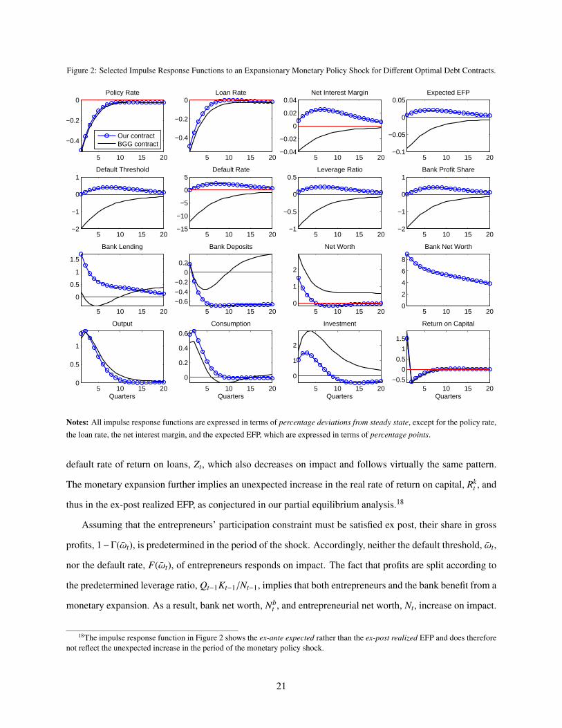
Figure 2: Selected Impulse Response Functions to an Expansionary Monetary Policy Shock for Different Optimal Debt Contracts.

5 10 15 20

−0.4

−0.2

0Policy Rate

Our contractBGG contract

5 10 15 20

−0.4

−0.2

0Loan Rate

5 10 15 20−0.04

−0.02

0

0.02

0.04Net Interest Margin

5 10 15 20−0.1

−0.05

0

0.05Expected EFP

5 10 15 20−2

−1

0

1Default Threshold

5 10 15 20−15

−10

−5

0

5Default Rate

5 10 15 20−1

−0.5

0

0.5Leverage Ratio

5 10 15 20−2

−1

0

1Bank Profit Share

5 10 15 20

0

0.5

1

1.5

Bank Lending

5 10 15 20

−0.6−0.4

−0.20

0.2

Bank Deposits

5 10 15 200

1

2

Net Worth

5 10 15 200

2

4

6

8

Bank Net Worth

5 10 15 200

0.5

1

Output

Quarters5 10 15 20

0

0.2

0.4

0.6

Consumption

Quarters5 10 15 20

0

1

2

Investment

Quarters5 10 15 20

−0.5

0

0.5

1

1.5

Return on Capital

Quarters

Notes: All impulse response functions are expressed in terms of percentage deviations from steady state, except for the policy rate,

the loan rate, the net interest margin, and the expected EFP, which are expressed in terms of percentage points.

default rate of return on loans, Zt, which also decreases on impact and follows virtually the same pattern.

The monetary expansion further implies an unexpected increase in the real rate of return on capital, Rkt , and

thus in the ex-post realized EFP, as conjectured in our partial equilibrium analysis.18

Assuming that the entrepreneurs’ participation constraint must be satisfied ex post, their share in gross

profits, 1−Γ(ωt), is predetermined in the period of the shock. Accordingly, neither the default threshold, ωt,

nor the default rate, F(ωt), of entrepreneurs responds on impact. The fact that profits are split according to

the predetermined leverage ratio, Qt−1Kt−1/Nt−1, implies that both entrepreneurs and the bank benefit from a

monetary expansion. As a result, bank net worth, Nbt , and entrepreneurial net worth, Nt, increase on impact.

18The impulse response function in Figure 2 shows the ex-ante expected rather than the ex-post realized EFP and does thereforenot reflect the unexpected increase in the period of the monetary policy shock.

21

From t + 1 on, the price of capital declines (not shown), implying capital losses to the entrepreneurs,

which are correctly anticipated by all economic agents under rational expectations (RE) in the absence of

further shocks. Nevertheless, the expected EFP for period t + 1 is above its steady-state value by about 0.7

basis points, which induces the bank to grant more loans both in absolute terms and relative to entrepreneurs’

net worth. As a consequence, the leverage ratio of entrepreneurs increases from the end of period t onwards

and peaks after five quarters at 0.21% above its steady-state value of 1.537.

This increase in borrower leverage allows the bank to demand a larger share of gross expected profits

realized in period t + 1 by raising the non-default rate of return on bank loans relative to the policy rate and

thus its net interest margin. Together with the implied default threshold, ωt+1, the expected default rate of

entrepreneurs, F (ωt+1), rises above its steady-state value. The maximum effect is reached after six quarters,

when the default threshold is 0.4% above its steady-state value of 0.35, and the default rate of entrepreneurs

is about 3 basis points above its steady-state value of 1.18%.

Now recall that the classic formulation of the CSV contract implies that entrepreneur i determines the

optimal amount of lending, Bit, and thus the leverage ratio for a predetermined amount of net worth, Ni

t , while

the “financial intermediary” only corresponds to a participation constraint. Assuming perfect diversification

across borrowers and the risk-sharing agreement in Bernanke et al. (1999), the passive financial intermediary

must break even in each realized state of the economy. Hence, there is no role for bank capital, Nbt = 0 ∀t,

and the entire windfall gain from the monetary expansion accrues to the entrepreneurs.

Figure 2 shows that, for the BGG contract, the entrepreneurs’ default threshold, default rate, and leverage

ratio as well as the expected EFP and net interest margin all decrease in response to a monetary expansion.

As a result, the partial equilibrium mechanism works in the opposite direction. In contrast with our contract

and the popular notion of a bank lending channel of monetary policy, the BGG contract furthermore implies

an initial contraction rather than an expansion of bank lending.

These crucial differences arise from the assumption in Bernanke et al. (1999) that a competitive financial

intermediary merely transforms household deposits into loans to entrepreneurs one for one. In contrast, the

monopolistic bank in our model retains a share of total profits, accumulates own net worth, and is thus able

to expand lending despite an even more pronounced and persistent reduction in deposits. The bank’s market

power and our assumption about aggregate risk sharing manifest themselves in a weaker pass-through from

monetary policy to the loan rate, relative to the BGG contract, and an increase rather than a decrease in the

net interest margin, which measures the expected profitability of bank loans.

22

The more pronounced increase in borrower net worth, Nt, as well as the contraction of aggregate bank

lending, Bt, imply the well-known decrease in the leverage ratio of entrepreneurs, QtKt/Nt = (Nt + Bt) /Nt,

in Bernanke et al. (1999), whereas the introduction of a risk channel in this paper facilitates a reduction in

deposits and an expansion of bank lending at the same time.

3.3.2. Risk Taking over the Business Cycle

A related question is whether our new mechanism matters for replicating the unconditional moments of

certain key variables over the business cycle. For this purpose, we augment our benchmark New Keynesian

DSGE model with four additional shock processes to total factor productivity, consumer preferences, and the

marginal efficiency of investment, as well as so-called “risk shocks” to the standard deviation of idiosyncratic

productivity draws, σω,t. While our calibration of the former three is based on the Maximum Likelihood

estimation results in Christensen and Dib (2008), unanticipated and anticipated risk shocks are calibrated in

line with the Bayesian estimation results in Christiano et al. (2014). Table C.1 in the Appendix summarizes

the calibration of additional shock processes.

Figure 3 plots the dynamic cross-correlations of selected variables and ratios with output based on the

theoretical model with our debt contract and the optimal debt contract in Bernanke et al. (1999), respectively,

against their empirical counterparts. To capture the variability at business cycle frequencies, both the data

and the simulated time series are HP-filtered with λ = 1, 600 before computing the unconditional moments.

Figure 3 illustrates that both models replicate the empirical cross-correlations of output and, especially,

investment reasonably well. Moreover, the simulated default rate of entrepreneurs tracks the correlation of

delinquency rates on business loans with output in the data surprisingly well. The importance of introducing

a risk channel becomes evident when considering bank-related variables. The model with our contract does

substantially better in replicating the empirical cross-correlations of banks’ SLOOS collateral requirements

and the net interest margin from Call Reports, in particular contemporaneously. The unconditional moments

of banks’ loan-to-deposit ratio and return on capital can only be assessed in our model in a meaningful way,

whereas, in Bernanke et al. (1999), the former is constant at unity, while the latter is not defined at all.

3.3.3. Sensitivity Analysis

An important question is whether the results in Figure 2 are sensitive to our choice of parameters. For

this reason, we perform a number of robustness checks within the range of commonly used parameter values.

First, our results are qualitatively and quantitatively robust to the absence of habit formation in consumption

23

Figure 3: Cross-Correlation of Selected Variables at Period t with Output at period t + τ, DSGE Model and Data.

−10 0 10

−0.5

0

0.5

1Output

τ−10 0 10

−0.5

0

0.5

Investment

τ−10 0 10

−0.4

−0.2

0

0.2

0.4

0.6

Loans/Deposits

τ−10 0 10

−0.4

−0.2

0

0.2

0.4

0.6

Net Income/Bank Equity

τ

−10 0 10

−0.5

0

0.5

Collateral Requirements

τ−10 0 10

−0.5

0

0.5

Delinquency Rate

τ−10 0 10

−0.5

0

0.5

Net Interest Margin

τ

DataOur contractBGG contract

Notes: Simulated time series and data are HP-filtered (λ = 1, 600). In the data, output corresponds to log(real GDP per capita),

investment to log(real investment expenditure per capita), loans/deposits to log(loans and leases in bank credit/demand deposits)

at commercial banks, net income/bank equity to Call Reports log(net interest income/total equity capital) for commercial banks in

the U.S., collateral requirements to the net percentage of domestic banks increasing collateral requirements for large and middle-

market firms, delinquency rate to delinquency rate on business loans; all commercial banks, and net interest margin to Call Reports

net interest margin for all U.S. banks.

(h = 0) as well as to the presence of price and wage indexation to past inflation by retailers and labor unions,

respectively.

Second, the results are qualitatively robust to the introduction of nonzero trend inflation. For example, an

annualized steady-state inflation rate of 1% marginally lowers the peak response of the borrowers’ leverage

ratio, default rate, and other contract variables while increasing their persistence somewhat.

Third, the absence of investment adjustment costs (φ = 0) substantially magnifies the impulse responses

of contract variables, such as the expected EFP, and increases therefore the risk channel of monetary policy.

With zero adjustment costs, however, the response of investment becomes unreasonably large. In contrast,

higher investment adjustment costs, the absence of variable capital utilization (σu → ∞), and the absence

of wage stickiness (ξw = 0) attenuate the risk channel quantitatively, albeit not qualitatively.

Fourth, our results are qualitatively robust to alternative specifications of a Taylor-type interest-rate rule,

such as a response to past or expected future rather than current inflation (compare Bernanke et al., 1999), a

response to past or expected future rather than current output, or a stronger response to deviations of inflation

24

from steady state.19 The only parameter that matters is the degree of interest-rate inertia in the Taylor rule.

Following a monetary expansion, higher inertia implies that the policy rate remains “too low for too long”

and magnifies thus the effect of the risk channel (see also Figure C.2 in the Appendix).

4. The Empirical Evidence

In the existing literature, evidence for a risk-taking channel of monetary policy on the asset side is mostly

confined to microeconomic loan-level data (see, e.g., Jimenez et al., 2014; Ioannidou et al., 2015; Paligorova

and Santos, 2017). When macroeconomic time series are used, the results are often ambiguous. Maddaloni

and Peydro (2011) exploit the cross-sectional variation in economic conditions across euro-area countries

to show that corporate banks soften their lending standards in response to low short-term interest rates and

that the impact on lending standards is amplified by the duration of relatively low interest rates. Since their

identification strategy rests on a common monetary policy stance in the euro area, it is not suitable for the

U.S., where they find little evidence for a risk channel of monetary policy. Using a rich panel of banking

data with 140 time series in a FAVAR model, Buch et al. (2014) find evidence in favor of asset-side risk

taking for small U.S. banks only. Importantly, Buch et al. (2014) use a different measure of asset risk – the

riskiness of new loans from the Survey of Terms of Business Lending of the U.S. Federal Reserve, which

restricts their sample period to 1997Q2-2008Q2.

Instead, we use the quantified qualitative survey measures of bank lending standards from the Federal

Reserve’s SLOOS, which are available from 1991Q1 onwards. Similar to Buch et al. (2014), we employ a

FAVAR model, which allows us to parsimoniously use the information in a large number of macroeconomic

time series, thereby reducing the risk of omitted-variable bias (see also Bernanke et al., 2005).20 We extract

the so-called factors from a comprehensive set of real economic activity measures including indicators of

production, investment, and employment. In order to be able to detect a risk channel of monetary policy,

we augment the macroeconomic and financial time series commonly used in the FAVAR literature by 19

measures of lending standards, such as the net percentage of banks increasing collateral requirements or

tightening loan covenants, for several categories of loans, borrowers, and banks. Figure 4 plots these lending

19Note that our results are not affected by a response of monetary policy to the so-called “output gap”, i.e. the deviation of actualfrom potential output, under flexible prices. Due to the neutrality of money, potential output is identical to steady-state output inthe absence of nominal rigidities.

20In Appendix F.1, we illustrate that the response of SLOOS lending standards to a monetary policy shock is not robust todifferent choices for the measure of real economic activity in a small-scale VAR model.

25

Figure 4: SLOOS Lending Standards and the Effective Federal Funds Rate, 1991Q1-2015Q4.

1991Q1 1995Q1 1999Q1 2003Q1 2007Q1 2011Q1 2015Q1−100

−50

0

50

100

Lend

ing

stan

dard

s: n

et p

erce

ntag

e of

ban

ks ti

ghte

ning

1991Q1 1995Q1 1999Q1 2003Q1 2007Q1 2011Q1 2015Q10

2

4

6

8

FF

R: p

erce

nt p

er a

nnum

Notes: See Appendix D for a detailed description of lending standard measures.

standards against the effective federal funds rate. Note that the substantial comovement in lending standards

over the sample period might be captured well even by a relatively small number of common factors.

4.1. The Econometric Specification

Suppose that the observation equation relating the N × 1 vector of informational time series, Xt, to the

K×1 vector of unobservable factors, Ft, and the M×1 vector of observable variables, Yt, with K + M << N,

is given byXt = Λ f Ft + ΛyYt + et, (19)

where Λ f is an N × K matrix of factor loadings of the unobservable factors, Λy is an N × M matrix of

factor loadings of the observable variables, and et is an N × 1 vector of error terms following a multivariate

normal distribution with mean zero and covariance matrix, R.

Suppose further that the joint dynamics of the unobserved factors in Ft and the observable variables in

Yt can be captured by the transition equation Ft

Yt

= Φ(L)

Ft−1

Yt−1

+ νt, (20)

where Φ(L) is a lag polynomial of order d and νt is a (K + M) × 1 vector of error terms following a

multivariate normal distribution with mean zero and covariance matrix, Q. The error terms in et and νt are

assumed to be contemporaneously uncorrelated.

26

Estimating the FAVAR model in (19) and (20) requires transforming the data to induce stationarity of

the variables.21 Our baseline sample contains quarterly observations for 1991Q1-2008Q2. While the start is

determined by the availability of the SLOOS measures of bank lending standards, we exclude the period after

2008, when U.S. monetary policy was effectively operating through the balance sheet of the Federal Reserve

rather than through the Federal Funds rate (compare Figure 4). The predominance of unconventional policy

measures would require a different strategy for identifying monetary policy shocks during this period.

Following Bernanke et al. (2005), we identify monetary policy shocks recursively, ordering the Federal

Funds rate last in equation (20). In our case, this implies that the unobserved factors do not respond to mon-

etary policy innovations within the same quarter, while the idiosyncratic components of the informational

time series in Xt are free to respond on impact.22 One could argue that senior loan officers take into account

the current monetary stance when deciding on their lending standards. Hence, it is important to note that the

SLOOS is conducted by the Federal Reserve, so that results are available before the quarterly meetings of

the Federal Open Market Committee (FOMC), in line with our identification scheme.

We estimate the FAVAR model in (19) and (20) by a one-step Bayesian approach, applying multi-move

Gibbs sampling to sample jointly from the latent factors and the model parameters. Appendix E provides

details on the prior distributions, the Gibbs sampler, and how we monitor the convergence of the latter. In

our baseline specification, we set the lag order of the transition equation to two quarters and consider the

Federal Funds rate as the only observable variable in (20), i.e. M = 1.23

To determine the appropriate number of unobservable factors in our FAVAR specification, we consult a

number of selection criteria, monitor the joint explanatory power of Ft and Yt for bank lending standards,

and check the robustness of our results by adding more factors. The tests of Onatski (2009) and Alessi et al.

(2010) point to three and five factors, respectively. Trying specifications with up to seven factors, we found

that our results were not affected qualitatively.24 In what follows, we therefore refer to the specification with

three unobservable factors as the baseline FAVAR model.

21The transformation of variables is detailed in Appendix D. Note that the measures of bank lending standards enter the FAVARmodel in (standardized) levels, i.e. without first-differencing or detrending, given that they are stationary by construction.

22Bernanke et al. (2005) apply the same recursive ordering to a FAVAR model in monthly data.23Results for lag orders one and three are very similar. Adding CPI as an observable variable (M = 2) does not affect our results.24Table F.1 in the Appendix reports the adjusted R2 for each of the 19 SLOOS measures with one, three, five, and seven

unobservable factors, illustrating that a small number factors is sufficient to capture the common comovement in lending standards.Our results are also consistent with the so-called “scree plot”, which plots the eigenvalues of Xt in descending order against thenumber of principal components. In our case, the scree plot displays a steep negative slope and a kink around the fifth principalcomponent, supporting the results based on the selection criteria and the robustness checks.

27

4.2. Results from the Structural FAVAR Model

4.2.1. Impulse Response Functions

Figure 5 plots the responses of selected variables from the theoretical DSGE model to an expansionary

monetary policy shock against their empirical counterparts from the benchmark FAVAR model with K = 3

latent factors. In order to facilitate a comparison of the theoretical and empirical impulse response functions,

the bank’s collateral requirements, bank profits, and investment are expressed in terms of their unconditional

standard deviations, while the policy rate and the bank’s net interest margin are converted to annualized basis

points, both in the DSGE and the FAVAR model. One period on the x-axis corresponds to one quarter.

In the theoretical model, the policy rate converges smoothly to its steady-state value, while the empirical

effective federal funds rate displays substantial overshooting about two years after the monetary expansion.

Hence, the initial increase in the empirical net interest margin is quickly reversed, turning into a marginally

significant decrease, while the response of the theoretical net interest margin remains positive throughout.

Despite this discrepancy in the transmission of the shock through interest rates and spreads, our theoretical

model is able to replicate the empirical impulse responses of bank lending standards, profits, and investment.

In the DSGE and the FAVAR model, banks significantly lower their collateral requirements in response

to an expansionary monetary policy shock, thus raising the demand for productive capital and investment.

Figure 5: Impulse Responses of Selected Variables to an Expansionary Monetary Policy Shock, DSGE Model and FAVAR Modelwith Three Unobserved Factors.

0 20−200

−150

−100

−50

0

50

100

150

200

250Policy Rate

Ann

ualiz

ed b

asis

poi

nts

Quarters0 20

−20

−10

0

10

20

30

40Net Interest Margin

Ann

ualiz

ed b

asis

poi

nts

Quarters0 20

−0.4

−0.3

−0.2

−0.1

0

0.1

0.2

0.3Collateral Requirements

Sta

ndar

d de

viat

ions

Quarters0 20

−0.6

−0.4

−0.2

0

0.2

0.4

0.6

0.8Bank Profit

Sta

ndar

d de

viat

ions

Quarters0 20

−0.4

−0.3

−0.2

−0.1

0

0.1

0.2

0.3Investment

Sta

ndar

d de

viat

ions

Quarters

DSGEFAVAR

Notes: In the FAVAR model, the effective federal funds rate is used as a measure of the monetary policy rate, the Call Reports net

interest margin for all U.S. banks as a proxy for the theoretical interest rate spread, the net percentage of domestic banks increasing

collateral requirements for large and middle-market firms as a measure of bank lending standards, the Call Reports net income for

commercial banks in the U.S. to measure bank profit, and the ISM Manufacturing: New Orders Index as a proxy for investment.

See Appendix D for a detailed description of the data. For the FAVAR model, median responses are plotted with pointwise 16th/84th

and 5th/95th percentiles.

28

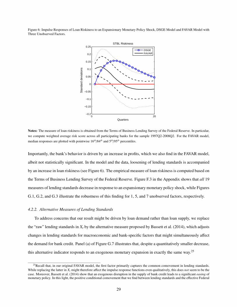
Figure 6: Impulse Responses of Loan Riskiness to an Expansionary Monetary Policy Shock, DSGE Model and FAVAR Model withThree Unobserved Factors.

0 20−0.2

−0.15

−0.1

−0.05

0

0.05

0.1

0.15

0.2

0.25STBL Riskiness

Sta

ndar

d de

viat

ions

Quarters

DSGEFAVAR

Notes: The measure of loan riskiness is obtained from the Terms of Business Lending Survey of the Federal Reserve. In particular,

we compute weighted average risk score across all participating banks for the sample 1997Q2-2008Q2. For the FAVAR model,

median responses are plotted with pointwise 16th/84th and 5th/95th percentiles.

Importantly, the bank’s behavior is driven by an increase in profits, which we also find in the FAVAR model,

albeit not statistically significant. In the model and the data, loosening of lending standards is accompanied

by an increase in loan riskiness (see Figure 6). The empirical measure of loan riskiness is computed based on

the Terms of Business Lending Survey of the Federal Reserve. Figure F.3 in the Appendix shows that all 19

measures of lending standards decrease in response to an expansionary monetary policy shock, while Figures

G.1, G.2, and G.3 illustrate the robustness of this finding for 1, 5, and 7 unobserved factors, respectively.

4.2.2. Alternative Measures of Lending Standards

To address concerns that our result might be driven by loan demand rather than loan supply, we replace

the “raw” lending standards in Xt by the alternative measure proposed by Bassett et al. (2014), which adjusts

changes in lending standards for macroeconomic and bank-specific factors that might simultaneously affect

the demand for bank credit. Panel (a) of Figure G.7 illustrates that, despite a quantitatively smaller decrease,

this alternative indicator responds to an exogenous monetary expansion in exactly the same way.25

25Recall that, in our original FAVAR model, the first factor primarily captures the common comovement in lending standards.While replacing the latter in Xt might therefore affect the impulse response functions even qualitatively, this does not seem to be thecase. Moreover, Bassett et al. (2014) show that an exogenous disruption in the supply of bank credit leads to a significant easing ofmonetary policy. In this light, the positive conditional comovement that we find between lending standards and the effective Federal

29

Figure 7: Impulse Responses of Alternative Measures of Lending Standards to an Expansionary Monetary Policy Shock.

0 20−0.4

−0.3

−0.2

−0.1

0

0.1

0.2

0.3

0.4(a) Adjusted Lending Standards

Quarters

Sta

ndar

d de

viat

ions

0 20−0.4

−0.3

−0.2

−0.1

0

0.1

0.2

0.3

0.4(b) SLOOS Risk Tolerance

Quarters

Sta

ndar

d de

viat

ions

0 20−0.4

−0.3

−0.2

−0.1

0

0.1

0.2

0.3

0.4(c) Excess Bond Premium

Quarters

Sta

ndar

d de

viat

ions

0 20−0.4

−0.3

−0.2

−0.1

0

0.1

0.2

0.3

0.4(d) NFCI Credit Subindex

Quarters

Sta

ndar

d de

viat

ions

Notes: Median responses with pointwise 16th/84th and 5th/95th percentiles, based on the FAVAR model with three unobserved

factors, where the 19 SLOOS lending standard measures have been replaced by (a) the credit supply indicator proposed by Bassett

et al. (2014); (b) the net percentage of domestic banks easing lending standards due to increased risk tolerance; (c) the excess

bond premium proposed by Gilchrist and Zakrajsek (2012); (d) the NFCI credit subindex published by the Federal Reserve Bank

of Chicago. See Appendix D for a detailed description of the data.

The SLOOS also asks senior loan officers for the reasons that induced them to adjust lending standards.

Among the latter, the category “risk tolerance” allows us to explicitly address the question whether banks’

risk appetite played any role when easing lending standards in response to a monetary expansion. Panel (b)

of Figure G.7 plots the (negative) impulse response function of the net percentage of domestic banks easing

lending standards due to increased risk tolerance. The finding of a statistically significant increase supports

our interpretation of banks’ easing of lending standards as a risk channel of monetary policy.

While the focus of our paper is on lending standards and collateral requirements, in particular, qualitative

surveys like the SLOOS can be criticized for being more prone to subjectiveness or intentional misreporting.

Hence, we also investigate the impulse responses of two market-based measures of the financial sector’s risk

attitude: the “excess bond premium” proposed by Gilchrist and Zakrajsek (2012) – a component of the “GZ

spread” that captures cyclical changes in the relationship between objective default risk and credit spreads

– and the credit subindex of the Chicago Fed’s National Financial Conditions Index (NFCI) – a composite

measure of credit conditions. Panels (c) and (d) of Figure G.7 illustrate that both the excess bond premium

and the NFCI credit component decrease significantly in response to an exogenous monetary expansion,

indicating an increase in “the effective risk-bearing capacity of the financial sector” (compare Gilchrist and

Zakrajsek, 2012) and thus an expansion in the supply of credit, consistent with the risk-taking channel of

Funds rate is unlikely to be contaminated by reverse causality from bank behavior to monetary policy.

30

monetary policy.

4.2.3. Robustness of Identifying Strategy

Barakchian and Crowe (2013) provide empirical evidence that U.S. monetary policy post 1988 became

more forward-looking, implying that a credible identification of exogenous monetary shocks must account

for policy makers’ expectations about future economic activity and price dynamics during our sample period.

While our benchmark specification of Xt already contains forward-looking variables, such as the S&P 500 or

business and consumer survey data, one could argue that the Board of Governors uses additional information

when forming its monetary policy decisions. For this reason, we include 13 quarterly time series from the

Philadelphia Fed’s Greenbook data set, expressed in terms of one-year-ahead expectations of average growth

rates, directly in the vector Xt and find that the impulse responses of lending standards to an expansionary

monetary policy shock are quantitatively very similar to those presented above and statistically significant

at the 10% level for 1, 3, and 5 factors. For 7 factors, our estimates become less precise, while the easing of

lending standards remains significant according to the error bands containing 68% of the probability mass.26

Moreover, we abandon the FAVAR model altogether in favor of a high-frequency identification approach.

Following Barakchian and Crowe (2013), we extract an alternative time series of monetary policy shocks

from daily changes in federal funds futures yields for different maturities around FOMC meeting dates.27

We then regress each variable of interest on P = 4 own lags as well as the contemporaneous and Q = 12

lagged observations of the quarterly aggregate of this monthly shock series in a distributed lag regression

model. Figure G.5 in the Appendix plots the impulse responses of selected variables from the theoretical

DSGE model to an expansionary monetary policy shock against their empirical counterparts and illustrates

that our findings in Figure 5 are qualitatively robust to the identifying strategy in Barakchian and Crowe

(2013). Note also that, based on the high-frequency identification of monetary policy shocks, the increase in

bank profits is statistically significant. As in the FAVAR, the loosening of lending standards is accompanied

by an increase in loan riskiness (see Figure G.6). The qualitative robustness carries over to all 19 SLOOS

lending standards measures and the alternative measures of the financial sector’s risk appetite in Figure G.7.

26The projections from the Fed’s Greenbook are released to the public with a lag of five years and are currently available up to2010Q4. For more details, see Table D.2 in the Appendix. All results are available from the authors upon request.

27The median correlation of the resulting shock series with the shock series based on the last 10,000 draws from the Gibbssampler for our baseline FAVAR model is 0.273 and highly statistically significant (see also Figure G.4 in the Appendix).

31

4.2.4. Extended Sample Period

Despite concerns that the effective Federal Funds rate represents an incomplete measure of monetary

policy at the zero lower bound (ZLB), we extend our sample period to 2015Q4 as a final robustness check.

In Appendix G.3, we reproduce Figures 5, G.7, and F.3 for the extended sample based on the FAVAR model

with three unobserved factors and the high-frequency identification approach. When including the ZLB

period, our theoretical model continues to replicate the empirical impulse responses of the effective Fed-

eral Funds rate, banks’ collateral requirements from SLOOS, and investment to a monetary policy shock.

For the FAVAR model, the responses of banks’ net interest margin and profits are imprecisely estimated

and tend toward the opposite direction, whereas the net interest margin’s response remains significantly

positive for the identifying strategy in Barakchian and Crowe (2013). At the same time, Figures G.10 and

G.11 show that all 19 SLOOS lending standards decrease significantly in response to a monetary expansion,

while Figures G.12 and G.13 indicate a significant easing of alternative measures of the financial sectors’

lending standards, regardless of the chosen identification.28 It is beyond the scope of this paper to identify

monetary policy shocks attributable to the unconventional monetary policy during the zero lower bound

period. Kurtzman et al. (2017) study the effect of large-scale asset purchase programs of the Federal Re-

serve and find loosening of lending standards and higher bank risk-taking measured by loan riskiness, thus

corroborating our baseline findings.

5. Concluding Remarks

In this paper, we reformulate the well-known application of Townsend’s (1979) CSV contract in Bernanke

et al. (1999) from the perspective of a monopolistic bank, which chooses the amount of risky lending against

borrower collateral subject to the participation constraint of a continuum of entrepreneurs. We assume that

both the bank and entrepreneurs are risk-neutral. While the bank can diversify any idiosyncratic default risk

of borrowers, it bears the aggregate risk. In partial equilibrium, the optimal debt contract yields a positive

relationship between the expected EFP and the borrower’s leverage ratio chosen by the bank. As a result,

an exogenous increase in the expected EFP induces the bank to lend more against a given amount of bor-

rower collateral in order to gain a larger “share of the pie”. At the same time, entrepreneurs become more

28The credit supply indicator proposed by Bassett et al. (2014) is only available until 2008Q2. For this reason, we omit it in ourrobustness checks for the extended sample.

32

leveraged and thus more likely to default ex post.

We then embed our version of the CSV contract in an otherwise standard New Keynesian DSGE model.

In contrast to the prior literature, an expansionary monetary policy shock leads to a hump-shaped increase in

the expected EFP and the bank’s net interest margin, which measures the profitability of loans. As a result,

our model predicts an increase in bank lending relative to borrower collateral, a higher leverage ratio, and

thus a higher expected default rate of entrepreneurs, in line with the risk channel of monetary policy (see,

e.g., Adrian and Shin, 2011; Borio and Zhu, 2012).

Using a FAVAR model and including measures of bank lending standards from the Federal Reserve’s

Senior Loan Officer Opinion Survey (SLOOS), we show that our theoretical model replicates the empirical

impulse responses of banks’ self-reported collateral requirements, their net interest margin and profits as

well as investment to a monetary policy shock both qualitatively and quantitatively. U.S. banks significantly

lower all 19 lending standards in response to an unexpected reduction in the effective Federal Funds rate.

This finding carries over to alternative measures of financial intermediaries’ risk appetite and is robust to the

high-frequency identification of monetary policy shocks in Barakchian and Crowe (2013).

While our results can be interpreted as robust evidence for an ex-ante risk channel of monetary policy

(i.e. lower lending standards), we do not show empirical evidence of ex-post risk taking (i.e. higher default

rates). The reason is that aggregate charge-off and delinquency rates are reported for the stock of loans and

leases at commercial banks. It is therefore unclear whether a defaulting loan was originated before of after

the monetary policy shock occurred. By tracking each loan in the Bolivian credit register from origination

to maturity, Ioannidou et al. (2015) show that lower overnight interest rates induce banks to commit larger

loan volumes with fewer collateral requirements to ex-ante riskier firms that are more likely to default ex

post. A similar analysis based on loan-level data is beyond the scope of this paper and left for future work.

33

6. References

Adrian, Tobias and Hyun Song Shin (2011). “Financial Intermediaries and Monetary Economics,” in: Fried-

man, B., Woodford, M. (Eds.), Handbook of Monetary Economics, Volume 3A.

Alessi, Lucia, Matteo Barogozzi, and Marco Capasso (2010). “Improved Penalization for Determining the

Number of Factors in Approximate Factor Models”, Statistics & Probability Letters 80: 1806-1813.

Barakchian, S. Mahdi and Christopher Crowe (2013). “Monetary policy matters: Evidence from new shocks

data,” Journal of Monetary Economics 60(8): 950-966.

Bassett, William F., Mary Beth Chosak, John C. Driscoll, and Egon Zakrajsek (2014). “Changes in bank

lending standards and the macroeconomy,” Journal of Monetary Economics 62(1): 23-40.

Basu, Susanto (1996). “Procyclical Productivity: Increasing Returns or Cyclical Utilization?” Quarterly

Journal of Economics 111(3): 719-751.

Bernanke, Ben S., Mark Gertler, and Simon Gilchrist (1999). “The Financial Accelerator in a Quantitative

Business Cycle Framework,” in: Taylor, J., Woodford, M. (Eds.), Handbook of Macroeconomics.

Bernanke, Ben S., Jean Boivin, and Piotr Eliasz (2005). “Measuring the Effects of Monetary Policy: A

FAVAR Approach,” Quarterly Journal of Economics 120(1): 387-422.

Board of Governors of the Federal Reserve System (U.S.), Senior Loan Officer Opinion Survey on Bank

Lending Practices, http://www.federalreserve.gov/boarddocs/SnLoansurvey/.

Board of Governors of the Federal Reserve System (U.S.), Survey of Terms of Business Lending,

https://www.federalreserve.gov/releases/e2/current/.

Borio, Claudio and Haibin Zhu (2012). “Capital regulation, risk-taking and monetary policy: A missing link

in the transmission mechanism?” Journal of Financial Stability 8(4): 236-251.

Buch, Claudia, Sandra Eickmeier, and Esteban Prieto (2014). “In search for yield? Survey-based evidence

on bank risk taking,” Journal of Economic Dynamics and Control 43: 12-30.

Carlstrom, C. and Timothy Fuerst (1997). “Agency Costs, Net Worth, and Business Fluctuations: A Com-

putable General Equilibrium Analysis,” American Economic Review 87(5): 893-910.

Chari, V. V., Patrick J. Kehoe, and Ellen R. McGrattan (2000). “Sticky Price Models of the Business Cycle:

Can the Contract Multiplier Solve the Persistence Problem?” Econometrica 68(5): 1151-1179.

Christensen, Ian and Ali Dib (2008). “The Financial Accelerator in an Estimated New Keynesian Model,”

Review of Economic Dynamics 11(1): 155–178.

Christiano, Lawrence J., Martin Eichenbaum, and Charles L. Evans (2005). “Nominal Rigidities and the

Dynamic Effects of a Shock to Monetary Policy,” Journal of Political Economy 113(1): 1-45.

Christiano, Lawrence J., Roberto Motto, and Massimo Rostagno (2014). “Risk Shocks,” American Eco-

nomic Review 104(1): 27-65.

34

Covas, Francisco and Wouter J. Den Haan (2012). “The Role of Debt and Equity Finance Over the Business

Cycle,” Economic Journal 122(565): 1262-1286.

Federal Reserve Bank of Philadelphia, Greenbook Data Sets, https://www.philadelphiafed.org/research-and-

data/real-time-center/greenbook-data.

Federal Reserve Bank of St. Louis, FRED, https://fred.stlouisfed.org.

Forni, Mario and Luca Gambetti (2014), “Sufficient information in structural VARs,” Journal of Monetary

Economics 66(1): 124-136.

Gale, Douglas and Martin Hellwig (1985). “Incentive-Compatible Debt Contracts: The One-Period Prob-

lem,” Review of Economic Studies 52(4): 647-663.

Gertler, Mark and Peter Karadi (2011). “A model of unconventional monetary policy,” Journal of Monetary

Economics 58(1): 17-34.

Gertler, Mark, Nobuhiro Kiyotaki, and Albert Queralto (2012). “Financial crises, bank risk exposure and

government financial policy,” Journal of Monetary Economics 59(S): S17-S34.

Gilchrist, Simon and Egon Zakrajsek (2012). “Credit Spreads and Business Cycle Fluctuations,” American

Economic Review 102(4): 1692-1720.

Ioannidou, Vasso, Steven Ongena, and Jose-Luis Peydro (2015). “Monetary Policy, Risk-Taking and Pricing:

Evidence from a Quasi-Natural Experiment,” Review of Finance 19(1): 95-144.

Jimenez, Gabriel, Steven Ongena, Jose-Luis Peydro, and Jesus Saurina (2014). “Hazardous Times for Mon-

etary Policy: What Do Twenty-Three Million Bank Loans Say about the Effects of Monetary Policy on

Credit Risk-Taking?” Econometrica 82(2): 463-505.

Kurtzman, Robert. J., Stephan Luck, and Tom Zimmermann (2017). “Did QE Lead Banks to Relax Their

Lending Standards? Evidence from the Federal Reserve’s LSAPs?,” Finance and Economics Discussion

Series 2017-093. Board of Governors of the Federal Reserve System (U.S.).

Levin, Andrew T., Fabio M. Natalucci, and Egon Zakrajsek (2004). “The Magnitude and Cyclical Behavior

of Financial Market Frictions,” Federal Reserve Board Finance and Economics Discussion Series 04-70.

Maddaloni, Angela and Jose-Luis Peydro (2011). “Bank Risk-taking, Securitization, Supervision, and Low

Interest Rates: Evidence from the Euro-area and the U.S. Lending Standards,” Review of Financial Studies

24(6): 2121-2165.

Onatski, Alexei (2009). “Testing Hypotheses about the Number of Factors in Large Factor Models,” Econo-

metrica 77(5): 1447-1479.

Paligorova, Teodora and Joao A.C. Santos (2017). “Monetary Policy and Bank Risk-Taking: Evidence from

the Corporate Loan Market,” Journal of Financial Intermediation 30: 35-49.

Petersen, Mitchell A. and Raghuram G. Rajan (1995). “The Effect of Credit Market Competition on Lending

Relatioships,” Quarterly Journal of Economics 110(2): 407-443.

35

Taylor, John B. (1993). “Discretion versus Policy Rules in Practice,” Carnegie-Rochester Conference Series

on Public Policy 39: 195-214.

Taylor, John B. (2007). “Housing and Monetary Policy,” Proceedings – Economic Policy Symposium –

Jackson Hole: 463-476.

Townsend, Robert M. (1979). “Optimal Contracts and Competitive Markets with Costly State Verification,”

Journal of Economic Theory 21(2): 265-293.

Valencia, Fabian (2014). “Monetary policy, bank leverage, and financial stability,” Journal of Economic

Dynamics and Control 47: 20-38.

36

Appendix A. The Optimal Loan Contract

This appendix provides details on the optimal financial contract, following the logic in Bernanke et al.

(1999). Given the different assumptions about the roles of borrowers and lenders, however, we deviate from

the latter, where this is necessary.

Appendix A.1. Without Aggregate Risk

In the absence of aggregate risk, the loan contract between the bank and entrepreneur i is only affected by

the entrepreneur’s idiosyncratic risk ωi. Consequently, the bank’s constrained profit maximization problem

can be formulated as in equation (6), where all terms are defined in the main text.

Given the borrower’s net worth, the bank chooses the volume of the loan and thus k. For any value of k,

the entrepreneur’s participation constraint (PC) pins down the default threshold ωi, which splits the expected

total profits from the investment project between the borrower and the lender. Given ωi, the non-default rate

of return on the loan to entrepreneur i, Zit+1, will then be determined by (3).

For notational convenience, we suppress any time subscripts and index superscripts throughout the ap-

pendix, while our aim remains to derive the properties of the optimal contract between the bank and en-

trepreneur i.

Appendix A.1.1. The EFP and Loan Supply

In what follows, we establish a positive relationship, k = ψ (s), ψ′ (s) > 0, between the external finance

premium (EFP) s ≡ Rk/R and the bank’s optimal choice of the capital/net worth ratio k ≡ QK/N. The

Lagrangian corresponding to the constrained profit-maximization problem in (6) is given by

L =[Γ (ω) − µG (ω)

]sk − (k − 1 − n) + λ [1 − Γ (ω)] sk − s ,

where n ≡ Nb/N and λ is the Lagrangian multiplier on the borrower’s PC. The corresponding first-order

conditions (FOCs) are

k :[Γ (ω) − µG (ω)

]s − 1 + λ [1 − Γ (ω)] s = 0,

ω :[Γ′ (ω) − µG′ (ω)

]sk − λΓ′ (ω) sk = 0,

λ : [1 − Γ (ω)] sk − s = 0.

Note that the assumptions made about Γ (ω) and µG (ω) imply that the bank’s expected profit share net

of expected default costs satisfies

Γ (ω) − µG (ω) > 0 for ω ∈ (0,∞) (A.1)

andlimω→0

Γ (ω) − µG (ω) = 0, limω→∞

Γ (ω) − µG (ω) = 1 − µ.

In order for the bank’s profits to be bounded in the case where the borrower defaults with probability one,

we therefore assume that s < 1/ (1 − µ) (compare Bernanke et al., 1999).

37

We further assume that ωh (ω) is increasing in ω, where h (ω) denotes the hazard rate f (ω) / [1 − F (ω)].29

Hence, there exists an ω∗ such that

Γ′ (ω) − µG′ (ω) = [1 − F (ω)][1 − µωh (ω)

]T 0 for ω S ω∗,

i.e., the bank’s expected net profit share reaches a global maximum at ω∗. Moreover, the above assumption

implies thatΓ′ (ω) G′′ (ω) − Γ′′ (ω) G′ (ω) =

∂ [ωh (ω)]∂ω

[1 − F (ω)]2 > 0 for all ω. (A.2)

Consider first the FOC w.r.t. ω, which implies that

λ (ω) =Γ′ (ω) − µG′ (ω)

Γ′ (ω).

Taking the partial derivative w.r.t. ω, we obtain

λ′ (ω) =Γ′ (ω)

[Γ′′ (ω) − µG′′ (ω)

]− Γ′′ (ω)

[Γ′ (ω) − µG′ (ω)

][Γ′ (ω)]2 .

=µ [Γ′′ (ω) G′ (ω) − Γ′ (ω) G′′ (ω)]

[Γ′ (ω)]2 < 0, (A.3)

because Γ′ (ω) = 1 − F (ω) > 0 and Γ′′ (ω) G′ (ω) − Γ′ (ω) G′′ (ω) < 0 from (A.2) for all ω.

Taking limits,limω→0

λ (ω) = 1, limω→ω∗

λ (ω) = 0.

In contrast to Bernanke et al. (1999), λ (ω) is therefore a decreasing function of the cutoff. This is due to the

fact that, while the bank’s expected share of total profits is increasing in ω, a higher default threshold also

implies a higher expected verification cost. At ω∗, the increase in the expected verification cost, µG′ (ω),

exactly offsets the increase in the bank’s expected gross profit share, Γ′ (ω). As a consequence, the shadow

value of loosening the borrower’s PC converges to zero as ω→ ω∗.

From the FOC w.r.t. k, we can furthermore define a function

ρ (ω) ≡1

Γ (ω) − µG (ω) + λ [1 − Γ (ω)]= s.

Taking the partial derivative w.r.t. ω, we obtain

ρ′ (ω) = −ρ (ω)2 Γ′ (ω) − µG′ (ω) + λ′ (ω) [1 − Γ (ω)] − λ (ω) Γ′ (ω)

= −ρ (ω)2

λ (ω) Γ′ (ω) + λ′ (ω) [1 − Γ (ω)] − λ (ω) Γ′ (ω)

= −ρ (ω)2︸ ︷︷ ︸<0

λ′ (ω)︸︷︷︸<0

[1 − Γ (ω)]︸ ︷︷ ︸>0

> 0, (A.4)

29Given that we borrow the definitions of Γ (ω) and Γ (ω)−µG (ω) from Bernanke et al. (1999), our assumption about the hazardrate and its implications are identical to those in their Appendix A.

38

where the second equality uses the FOC w.r.t. ω. In the limit, as ω goes to 0 and ω∗, respectively,

limω→0

ρ (ω) = 1 (due to limω→0

λ (ω) = 1 and limω→0

G (ω) = 0),

limω→ω∗

ρ (ω) =1

Γ (ω∗) − µG (ω∗)≡ s∗ (due to lim

ω→ω∗λ (ω) = 0).

Accordingly, there is a one-to-one mapping between the optimal cutoff, ω, and the premium on external

funds, s, as in Bernanke et al. (1999). Inverting the function s = ρ (ω), we can therefore express the cutoff

as ω = ω (s), where ω′ (s) > 0 for s ∈ (1, s∗).

From the FOC w.r.t. λ, i.e. the borrower’s PC, we finally define

Ψ (ω) =1

1 − Γ (ω)= k.

Taking the partial derivative w.r.t. ω, we obtain

Ψ′ (ω) = −Ψ (ω)2 [−Γ′ (ω)

]= Ψ (ω)2︸ ︷︷ ︸

>0

[1 − F (ω)]︸ ︷︷ ︸>0

> 0. (A.5)

Hence, the qualitative implications are the same as in Bernanke et al. (1999). Taking limits,

limω→0

Ψ (ω) = 1, limω→ω∗

Ψ (ω) =1

1 − Γ (ω∗)< ∞.

Combining k = Ψ (ω) and ω = ω (s), where Ψ′ (ω) > 0 and ω′ (s) > 0, we can express the capital/net worth

ratio, k = QK/N, as a function k = ψ (s), where ψ′ (s) > 0 for s ∈ (1, s∗).

Appendix A.1.2. Proof of Interior Solution

Bernanke et al. (1999) use a general equilibrium argument to justify their assumption of an interior

solution, i.e. an optimal contract with ω < ω∗ and s < s∗. In particular, they argue that “as s approaches

s∗ from below, the capital stock becomes unbounded. In equilibrium this will lower the excess return s.”

(compare Bernanke et al., 1999, p.1384).

Here, we employ an analytical argument instead. Recall that the lender’s iso-profit curves (IPC) and the

borrower’s participation constraint (PC) in (k, ω)-space can be written as

kIPC =πb − 1 − n[

Γ (ω) − µG (ω)]

s − 1, (A.6)

kPC ≥1

1 − Γ (ω), (A.7)

where πb denotes an arbitrary level of bank profits.

Recall further that, in (k, ω)-space, the optimal contract is determined by the tangential point of the

borrower’s PC with the lowest IPC of the lender. Consider first the borrower’s PC in (A.7). Since Γ′ (ω) > 0,

kPC is a strictly increasing function for any ω ∈ [0,∞), so that the borrower’s PC has a positive slope

everywhere in (k, ω)-space.

Consider next the lender’s IPC in (A.6). Taking the partial derivative of kIPC w.r.t. ω,

39

∂k∂ω

∣∣∣∣∣IPC

=(1 − πb + n

) [Γ′ (ω) − µG′ (ω)

]s[

Γ (ω) − µG (ω)]

s − 12

> 0 for ω ∈ [0, ω∗)

= 0 for ω = ω∗

< 0 for ω ∈ (ω∗,∞)

.

Accordingly, the lender’s IPC has a positive slope in (k, ω)-space left of ω∗ and a negative slope right of ω∗.

Since the optimal contract requires that

∂k∂ω

∣∣∣∣∣IPC

=∂k∂ω

∣∣∣∣∣PC,

at the tangential point, and we already know that

∂k∂ω

∣∣∣∣∣PC

=Γ′ (ω)

[1 − Γ (ω)]2 > 0 for ω ∈ [0,∞)

the optimal default threshold can only lie in ω ∈ [0, ω∗), which guarantees an interior solution to the bank’s

constrained profit maximization problem.30

This completes the proof.

Appendix A.1.3. Proof of Uniqueness

As shown above, the tangential point of the borrower’s participation constraint (PC) and the lender’s

iso-profit curve (IPC) is located on the interval [0, ω∗). Uniqueness requires that there is exactly one such

point, i.e., we need to show that there exists only one ω that satisfies both

kPC =1

1 − Γ (ω)=

πb − 1 − n[Γ (ω) − µG (ω)

]s − 1

= kIPC (A.8)

and∂k∂ω

∣∣∣∣∣PC≡

Γ′ (ω)

[1 − Γ (ω)]2 =

(1 − πb + n

)s[Γ′ (ω) − µG′ (ω)

][Γ (ω) − µG (ω)

]s − 1

2 ≡∂k∂ω

∣∣∣∣∣IPC

, (A.9)

as the levels of k as well as the slopes implied by the PC and the IPC are identical at the point of tangency.

In what follows, we suppress the dependence of Γ (ω) and G (ω) on their argument ω for notational ease.

Note that (A.8) and (A.9) can be merged into a single condition that must hold at the tangential point:

Γ′ − µG′

Γ′=

1 − πb + ns

. (A.10)

Given that Γ′ = 1 − F , 0 on [0, ω∗), we can rewrite (A.10) as

1 −µG′

Γ′=

1 − πb + ns

⇔G′

Γ′=

1µ

(1 −

1 − πb + ns

),

the right-hand side of which is constant and thus a horizontal line in (k, ω)-space.

Partially differentiating the left-hand side with respect to ω yields

30Note that our line of argument equally applies to the formulation of the financial contract in Bernanke et al. (1999), likewiseguaranteeing an interior solution.

40

∂ (G′/Γ′)∂ω

=G′′Γ′ − Γ′′G′

(Γ′)2 > 0 for all ω from (A.2).

Given that the left-hand side is monotonically increasing in ω, it can cross the horizontal line defined by

the right-hand side at no more than one point on [0, ω∗), yielding a unique point of tangency between the

borrower’s PC and the lender’s IPC.31

This completes the proof.

Appendix A.2. With Aggregate Risk

In the presence of aggregate risk, the loan contract between the bank and entrepreneur i is affected by

the entrepreneur’s idiosyncratic risk, ωit+1, as well as by the ex-post realization of Rk

t+1. In this appendix, we

establish a positive relationship between the entrepreneur’s capital/net worth ratio, kit ≡ QtKi

t/Nit , and the

ex-ante expected external finance premium (EFP), st ≡ EtRkt+1/R

nt . Again, we suppress time subscripts and

index superscripts for notational convenience.

Following Bernanke et al. (1999), it is convenient to write total profits per unit of capital expenditures

as uωRk, where u denotes an aggregate shock to the gross real rate of return on capital, while ω continues

to denote the entrepreneur’s idiosyncratic productivity shock, where E (u) = E (ω) = 1. Using definitions

from the main text and Appendix Appendix A.1, we can rewrite the bank’s constrained profit maximization

problem in equation (6) as

maxk,ω

E[

Γ (ω) − µG (ω)]usk − (k − 1 − n)

s. t. E [1 − Γ (ω)] usk − us ≥ 0.

The corresponding Lagrangian,

L = E[

Γ (ω) − µG (ω)]usk − (k − 1 − n) + λ ([1 − Γ (ω)] usk − us)

,

yields the following first-order conditions (FOCs):

k : E[

Γ (ω) − µG (ω)]us − 1 + λ [1 − Γ (ω)] us

= 0,

ω : E[

Γ′ (ω) − µG′ (ω)]usk − λΓ′ (ω) usk

= 0,

λ : E [1 − Γ (ω)] usk − us = 0.

As discussed in the main text, we assume that the borrower’s participation constraint (PC) is satisfied ex

post, i.e. for each realization of u. As a consequence, ω and any function thereof, such as Γ (ω) and Γ′ (ω),

for example, is independent of the realization of u. Using this assumption, the above FOCs simplify to

k : E[

Γ (ω) − µG (ω)]us + λ [1 − Γ (ω)] us

= 1,

ω :[Γ′ (ω) − µG′ (ω)

]= λΓ′ (ω) ,

λ : [1 − Γ (ω)] k = 1.

31Note that G′/Γ′ is defined on ω ∈ [0,∞) and takes values on [0,∞). For this reason, the intersection between G′/Γ′ and[1 −

(1 − πb + n

)/s

]/µ exists for πb > 1 + n − s.

41

Partially differentiating the borrower’s ex-post PC w.r.t. k and ω, respectively, we obtain

∂

∂k= 1 − Γ (ω) − Γ′ (ω) k

∂ω

∂k= 0 ⇒

∂ω

∂k=

1 − Γ (ω)Γ′ (ω) k

> 0

and∂

∂s= −Γ′ (ω) k

∂ω

∂s= 0 ⇒

∂ω

∂s= 0.

Furthermore defining Υ (ω) ≡ Γ (ω) − µG (ω) + λ [1 − Γ (ω)], total differentiation of the FOC w.r.t. k yields

E

uΥ (ω) + usΥ′ (ω)(∂ω

∂sds +

∂ω

∂kdk

)= 0

⇔ E

usΥ′ (ω)∂ω

∂k

dk = −E

uΥ (ω) + usΥ′ (ω)

∂ω

∂s

ds

⇒dkds

= −E

uΥ (ω) + usΥ′ (ω) ∂ω∂s

E

usΥ′ (ω) ∂ω∂k

= −E uΥ (ω)

EusΥ′ (ω) ∂ω∂k

> 0,

where the final equality makes use of our previous results that ∂ω/∂k > 0, ∂ω/∂s = 0, and

Υ′ (ω) = Γ′ (ω) − µG′ (ω) − λ (ω) Γ′ (ω)︸ ︷︷ ︸= 0 from the FOC w.r.t. ω

+λ′ (ω) [1 − Γ (ω)] = λ′ (ω) k−1 < 0.

Similar to Bernanke et al. (1999), the optimal loan contract therefore implies a positive relationship between

the borrower’s capital/net worth ratio and the ex-ante expected EFP even in the presence of aggregate risk.

This completes the proof.

Appendix A.3. Heuristic Argument for our Risk-Sharing Agreement

Suppose that Zit was predetermined and thus acyclical in period t + 1. Given that Bi

t and QtKit are also

predetermined in t + 1, the definition of the default threshold in (3) implies that ωit+1 is a strictly convex,

decreasing function in Rkt+1 ∀Zi

t ,Rkt+1 > 0.32 Accordingly, an unexpected decrease in Rk

t+1 raises ωit+1 by

more than an equivalent unexpected increase in Rkt+1 lowers ωi

t+1, i.e., symmetric fluctuations in Rkt+1 imply

asymmetric fluctuations in the default threshold and thus in the default rate of entrepreneurs, even if the

idiosyncratic productivity shocks were uniformly distributed. This asymmetry is amplified if ωit+1 follows

a log-normal distribution with ωit+1 in the left tail of the distribution, as we assume below. Since default

imposes a resource cost on the economy in this model, any (unexpected) cyclicality of ωit+1 over the business

cycle is undesirable. Our risk-sharing agreement, where the bank bears the aggregate risk and hence ωit+1 is

acyclical on impact, eliminates the share of the monitoring cost that is due to the asymmetric fluctuations in

entrepreneur default.

32Recall that Zit and Rk

t+1 are the gross non-default rates of return on a loan to entrepreneur i and per unit of capital, respectively.

42

Appendix B. The General Equilibrium Model

The general equilibrium model comprises eight types of economic agents: A representative household,

a representative capital goods producer, a representative intermediate goods producer, a continuum of mo-

nopolistically competitive retailers, a continuum of monopolistically competitive labor unions, a continuum

of perfectly competitive entrepreneurs, a monopolistic bank, and a monetary authority.

Appendix B.1. Entrepreneurs

At the end of period t, entrepreneurs use their accumulated net worth, Nt, to purchase productive capital,

Kt, from capital goods producers at a price Qt in terms of the numeraire. To finance the difference between

their net worth and total capital expenditures, QtKt, entrepreneurs must borrow an amount Bt = QtKt − Nt

in real terms from banks, where variables without an index superscript denote economy-wide aggregates.

The entrepreneur decides on the degree of capital utilization ut and rents part of capital services utKt−1

to the intermediate goods producers (introduced below). The revenue from selling the capital services is

rkt utKt−1 and the cost (in real terms) of adjusting the capital utilization rate is a(ut)Kt−1, where we assume

a′ > 0 and a′′ > 0. The optimization problem of the entrepreneur is given by:

maxut

[rk

t ut − a(ut)]ωKt−1

In the aggregate optimum, i.e. averaged over all entrepreneurs, it must hold that

rkt = a′(ut). (B.1)

As in Christiano et al. (2014), we employ the following functional form for the adjustment cost function of

the capital utilization rate:

a(ut) =rk

ss

σu

[exp σu(ut − 1) − 1

], (B.2)

where rkss refers to the steady-state rental rate of capital services.

The aggregate real rate of return per unit of capital in period t depends on the real rental rate of capital

services, rkt ut, and the capital gain of the non-depreciated capital stock, (1 − δ)Kt−1, between t − 1 and t in

real terms, net of capital utilization adjustment costs a(ut):

Rkt =

rkt ut + (1 − δ)Qt − a(ut)

Qt−1. (B.3)

A continuum of risk-neutral entrepreneurs, indexed i ∈ [0, 1], is hit by an idiosyncratic disturbance ωit in

period t. As a result, the ex-post rate of return of entrepreneur i per unit of capital equals ωitR

kt . Following

Bernanke et al. (1999), we assume that ωit is i.i.d. across time t and across entrepreneurs i, with a continuous

and differentiable cumulative distribution function F(ω) over a non-negative support, where Eωi

t

= 1 ∀t

and the corresponding hazard rate h(ω) ≡ f (ω) / [1 − F (ω)] satisfies ∂ωh(ω)/∂ω > 0.

In contrast to Bernanke et al. (1999) and variations thereof, we assume that entrepreneurs can operate

even in financial autarky by purchasing QtKt = Nt in period t. In order for an entrepreneur to accept a loan

43

offer, the terms of the loan, i.e. the amount Bt and the nominal non-default rate of return, Zt, must be such

that the entrepreneur expects to be no worse off than in financial autarky. Assuming constant returns to scale

(CRS), the distribution of net worth, Nit , across entrepreneurs is irrelevant. As a consequence, the aggregate

version of the participation constraint in equation (4) can be written as

Et

∫ ∞

ωt+1

ωRkt+1QtKt −

Zt

πt+1dF(ω)

≥ Et

Rk

t+1

Nt, (B.4)

where the expectation is over Rkt+1, and ωt+1 denotes the expected default threshold in period t + 1, defined

by Etωt+1Rk

t+1

QtKt ≡ Et Zt/πt+1 Bt.

Using the definition of ωt+1 to substitute out Et Zt/πt+1 and expressing the aggregate profit share of

entrepreneurs in period t as 1 − Γ (ωt), equation (B.4) can equivalently be written as

Et[1 − Γ (ωt+1)] Rk

t+1

QtKt ≥ Et

Rk

t+1

Nt. (B.5)

Note that the ex-post realized value of Γ (ωt+1) generally depends on the realization of Rkt+1 through ωt+1.

Similar to Bernanke et al. (1999), we assume that this constraint must be satisfied ex post. Implicit in this

is the assumption that Rkt+1 is observed by both parties without incurring a cost, and that the non-default

repayment, Zt, can thus be made contingent on the aggregate state of the economy.

In order to avoid that entrepreneurial net worth grows without bound, we assume that an exogenous

fraction (1 − γe) of the entrepreneurs’ share of total realized profits is consumed in each period.33 As a

result, entrepreneurial net worth at the end of period t evolves according to

Nt = γe [1 − Γ(ωt)] Rkt Qt−1Kt−1. (B.6)

To sum up, the entrepreneurs’ equilibrium conditions comprise the real rate of return per unit of capital

in (B.3), the ex-post participation constraint in (B.5), the evolution of entrepreneurial net worth in (B.6),

and the real amount borrowed, Bt = QtKt − Nt. Moreover, the definition of the expected default threshold,

Etωt+1, determines the expected non-default repayment per unit borrowed by the entrepreneurs, Et Zt/πt+1.

Appendix B.1.1. Risk Shocks

We follow Christiano et al. (2014) to introduce risks shock, σω,t, into the model, which capture the extent

of cross-sectional dispersion in ω. Risk shocks follow an AR(1)-process with autocorrelation coefficient ρσand mean-zero normally distributed disturbances, uσt . To incorporate both unanticipated and anticipated

components of risk shocks, we adopt the following representation from Christiano et al. (2014):

log uσt = ξ0,t + ξ1,t−1 + · · · + ξp,t−p,

33In the literature, it is common to assume that an exogenous fraction of entrepreneurs “dies” each period and consumes its networth upon exit. The dynamic implications of either assumption are identical.

44

where p = 8, ξ0,t denotes the unanticipated component, while ξ j,t, j > 0, are so-called “news” components.

We assume the following correlation structure:

ρ[i, j]ξ =

Eξi,tξi,t√(Eξ2

i,t

) (Eξ2

i,t

) , i, j = 0, . . . , p, (B.7)

where ρ[i, j]ξ ∈ [−1, 1]. For parsimony, the standard deviation of the anticipated component is equal to σσ,

while the standard deviations of all news components are assumed to be identical and equal to σξ.

Appendix B.2. The Bank

For tractability, we assume a single monopolistic financial intermediary, which collects deposits from

households and provides loans to entrepreneurs. In period t, this bank is endowed with net worth or bank

capital Nbt . Abstracting from bank reserves or other types of bank assets, the balance sheet identity in real

terms is given by equation (1). The CSV problem in Townsend (1979) implies that, if entrepreneur i defaults

due to ωitR

kt Qt−1Ki

t−1 < (Zit−1/πt)Bi

t−1, the bank incurs a proportional cost µωitR

kt Qt−1Ki

t−1 and recovers the

remaining return on capital, (1 − µ)ωitR

kt Qt−1Ki

t−1.

In period t, the risk-neutral bank observes entrepreneurs’ net worth, Nit , and makes a take-it-or-leave-it

offer to each entrepreneur i. As a consequence, it holds a perfectly diversified loan portfolio between period

t and period t +1. Although the bank can thus diversify away any idiosyncratic risk arising from the possible

default of entrepreneur i, it is subject to aggregate risk through fluctuations in the ex-post rate of return on

capital, Rkt+1, and the aggregate default threshold, ωt+1. In order to be able to pay the risk-free nominal

rate of return Rnt on deposits in each state of the world, the bank must have sufficient net worth to protect

depositors from unexpected fluctuations in Rkt+1.

Now consider the bank’s problem of making a take-it-or-leave-it offer to entrepreneur i with net worth Nit

in period t. The contract offered by the bank specifies the real amount of the loan, Bit, and the nominal gross

rate of return in case of repayment, Zit . Given that Ni

t is predetermined at the end of period t, the bank’s choice

of Bit also determines the entrepreneur’s total capital expenditure, QtKi

t = Bit + Ni

t . Moreover, given QtKit

and Nit , the bank’s choice of Zi

t implies an expected default threshold Etωt+1 through Etωt+1Rk

t+1

QtKt ≡

Et Zt/πt+1 Bt. Hence, we can equivalently rewrite the bank’s constrained profit-maximization problem for

a loan to entrepreneur i as

maxKi

t ,ωit+1

Et

[Γ(ωi

t+1

)− µG

(ωi

t+1

)]Rk

t+1QtKit −

Rnt

πt+1

(QtKi

t − Nit − Nb,i

t

), (B.8)

where Γ(ωi

t

)≡

∫ ωit

0 ωdF(ω) + ωit

[1 − F

(ωi

t

)], µG

(ωi

t

)≡ µ

∫ ωit

0 ωdF (ω), and Nb,it denotes the share of total

bank net worth assigned to the loan to entrepreneur i, subject to the participation constraint in (4).

The corresponding first-order conditions with respect toKi

t , Etωit+1, λ

b,it

, where λb,i

t denotes the ex-post

45

value of the Lagrange multiplier on the participation constraint, are given by

Kit : Et

[Γ(ωi

t+1) − µG(ωit+1) + λb,i

t

(1 − Γ(ωi

t+1))]

Rkt+1

= Et

Rn

t

πt+1

, (B.9)

Etωit+1 : Et

[Γ′(ωi

t+1) − µG′(ωit+1)

]Rk

t+1

= Et

λb,i

t Γ′(ωit+1)Rk

t+1

, (B.10)

λb,it :

[1 − Γ(ωi

t+1)]

Rkt+1QtKi

t = Rkt+1Ni

t . (B.11)

Following Bernanke et al. (1999), we show in Appendix Appendix A.2 that the optimal debt con-

tract between entrepreneur i and the bank implies a positive relationship between the expected EFP, st ≡

EtRk

t+1πt+1/Rnt

, and the optimal capital/net worth ratio, ki

t ≡ QtKit/N

it .

Here, instead, we go beyond this “reduced-form” result and utilize the entire structure inherent in the

first-order conditions. Note that (B.9) equates the expected marginal return of an additional unit of capital

to the bank and the entrepreneur to the expected marginal cost of an additional unit of bank deposits in real

terms. Assuming that the participation constraint is satisfied ex post, this implies a positive relationship

between EtRk

t+1πt+1/Rn

t and Etωi

t+1

. Moreover, (B.11) equates the entrepreneur’s expected payoff with

and without the bank loan and implies a positive relationship between Etωi

t+1

and QtKi

t/Nit .

34 Together,

these two conditions determine the positive ex-ante relationship between the expected EFP in period t + 1

and the leverage ratio chosen by the bank in period t, while the first-order condition with respect to Etωi

t+1

pins down the ex-post value of the Lagrange multiplier, λb,i

t .

Given Nit , QtKi

t , and EtRk

t+1

, the definition of the expected default threshold, Et

ωi

t+1

, implies an

expected non-default real rate of return on the loan to entrepreneur i, EtZi

t/πt+1, while the same equation

evaluated ex post determines the actual non-default repayment conditional on Nit , QtKi

t , Etωi

t+1

, and the

realization of Rkt+1.

By the law of large numbers, Γ(ωi

t

)− µG

(ωi

t

)denotes the bank’s expected share of total period-t profits

(net of monitoring costs) from a loan to entrepreneur i as well as the bank’s realized profit share from its

diversified loan portfolio of all entrepreneurs. Accordingly, we can rewrite the bank’s aggregate expected

profits in period t + 1 as

EtVbt+1 = Et

[Γ (ωt+1) − µG (ωt+1)

]Rk

t+1QtKt −Rn

t

πt+1

(QtKt − Nt − Nb

t

), (B.12)

where the expectation is over possible realizations of Rkt+1 and πt+1, while Vb

t+1 is free of idiosyncratic risk.

The entrepreneurs’ participation constraint in (B.5) implies that ωt+1 and thus[Γ (ωt+1) − µG (ωt+1)

]are

predetermined in period t + 1. In order to keep the problem tractable, we assume that aggregate risk is small

34This becomes evident, when we use the ex-post assumption that Rkt+1 and ωt+1 are uncorrelated and rewrite (B.11) as

[1 − Γ(ωi

t+1)]≥

N it

QtKit≡

1ki

t,

i.e., entrepreneur i’s expected return on capital with the loan relative to financial autarky must be no smaller than the entrepreneur’s“skin in the game”. Since

[1 − Γ(ωi

t+1)]

is strictly decreasing in Et

ωi

t+1

, the participation constraint implies a positive relationship

between Et

ωi

t+1

and ki

t.

46

relative to the bank’s net worth, Nbt , so that bank default never occurs in equilibrium.

In order to avoid that its net worth grows without bound, we assume that an exogenous fraction (1 − γb)

of the bank’s share of total realized profits is consumed each period.35 As a result, bank net worth at the end

of period t evolves according to

Nbt = γbVb

t . (B.13)

Appendix B.3. Households

The representative household is risk-averse and derives utility from a Dixit-Stiglitz aggregate of imper-

fectly substitutable consumption goods,

Ct =

[∫ 1

0Ct( j)

εp−1εp d j

] εpεp−1

. (B.14)

Households have an infinite planning horizon and discount their future expected utility with the subjective

discount factor β < 1. They can transfer wealth intertemporally by saving in terms of bank deposits, which

pay the risk-free nominal return Rnt between t and t + 1.36 We allow for habit formation in consumption.

Households supply homogenous labor to the monopolistically competitive labor unions, which differentiate

labor at no cost and set nominal wages. The household’s constrained optimization problem can be summa-

rized as

maxCt ,ht ,Dt

E0

∞∑t=0

βtet

(Ct/Ch

t−1

)1−σ

1 − σ− χ

h1+ 1

η

t

1 + 1η

,Ct + Dt + rtat =

at−1

πt+

Rnt

πtDt−1 + hd

t

∫ 1

0wm

t

(wm

t

wt

)−εw

dm + Πt, (B.15)

where Dt are real deposits, at is the real payoff of nominal state-contingent assets, rt is the stochastic discount

factor between period t and t + 1, πt = Pt/Pt−1 is the gross inflation rate, and Pt ≡

[∫ 10 Pt( j)1−εpd j

] 11−εp

is the

corresponding aggregate price index. Πt denotes net lump-sum transfers of profits to the household from

the retailers and labor unions, whereas hdt

∫ 10 wm

t

(wmt

wt

)−εwdm is the real wage income of the household. The

parameter h determines the strength of habit formation, while the preference shocks et evolves according to

log et = ρe log et−1 + εet , εe

t ∼ N(0, σ2e).

The first-order conditions with respect to Ct,Dt, where λt denotes the Lagrange multiplier of the budget

35Alternatively, one could think of this “consumption” as a distribution of dividends to share holders or bonus payments to bankmanagers, which are instantaneously consumed.

36Note that deposits are risk-free, as long as the bank carries sufficient net worth to shield its depositors from fluctuations in theaggregate return on capital. Assuming that the return on deposits is risk-free in real terms, i.e. that the bank compensates depositorsalso for unexpected fluctuations in the rate of inflation, does not affect our result qualitatively.

47

constraint, are

Ct : et

Ct

Cht−1

1−σ

C−1t − βhEt

et+1

(Ct+1

Cht

)1−σ

C−1t

= λt,

Dt : λt = βEt

λt+1

Rnt

πt+1

.

We discuss the choice of the optimal labor supply below in Subsection Appendix B.7, jointly with the labor

unions’ choice of the optimal wage rate.

Appendix B.4. Capital Goods Producers

After production in period t has taken place, capital producers purchase the non-depreciated capital

stock from entrepreneurs, invest in a Dixit-Stiglitz aggregate of imperfectly substitutable investment goods,

It ≡

[∫ 10 It( j)

εp−1εp d j

] εpεp−1

, and sell the new stock of capital to entrepreneurs at the relative price Qt. We assume

that turning final output into productive capital, i.e. gross investment, is costly due to possible disruptions of

the production process, replacement of installed capital, or learning. The accumulation of physical capital

can then be written as

Kt = (1 − δ)Kt−1 + xt

[1 − S

(It

It−1

)]It, (B.16)

where S(

ItIt−1

)=

φ2

(It

It−1− 1

)2, S (1) = S ′(1) = 0, and S ′′(1) = φ (compare, e.g., Christiano et al., 2005).

We assume that an investment-specific shock, xt, affects the production of capital goods and that this shock

follows an AR(1)-process:

log xt = ρx log xt−1 + εxt , εx

t ∼ N(0, σ2x).

The profit-maximization problem of the representative capital goods producer, subject to the capital

accumulation equation in (B.16), is given by

maxIt

∞∑s=0

βs Qt+s[Kt+s − (1 − δ)Kt+s−1] − It+s ,

while the corresponding FOC with respect to investment in period t is given by

Qt xt

1 − φ2(

It

It−1− 1

)2

− φ

(It

It−1− 1

)It

It−1

+ βφEt

Qt+1xt+1

(It+1

It− 1

) (It+1

It

)2 = 1. (B.17)

Appendix B.5. Intermediate Goods Producers

Intermediate goods producers rent the productive capital stock from entrepreneurs and hire labor from

households, paying a competitive rental rate on capital services and a wage rate determined in the labor mar-

ket, respectively. To convert capital and labor into intermediate or wholesale goods, they use the following

Cobb-Douglas production function:

Yt = AtKαt h1−α

t ,

48

where At denotes a stationary shock to total factor productivity (TFP) that follows the AR(1)-process

log At = ρa log At−1 + εat , εa

t ∼ N(0, σ2a).

Note that the first input argument of the production function, Kt, stands for capital services, defined as

Kt = utKt−1, (B.18)

where ut is the utilization rate of capital in period t chosen by entrepreneurs.

Suppose that the price of the homogeneous wholesale good in terms of the numeraire is 1/Xt, so that the

gross flexible-price markup of retail goods over the wholesale good is Xt. The static optimization problem

of the intermediate goods producer can then be summarized as

maxKt ,ht

1Xt

AtKαt h1−α

t − rkt Kt − wtht,

which yields the following FOCs:

Kt : Xtrkt = α

Yt

Kt,

ht : Xtwt = (1 − α)Yt

ht.

Appendix B.6. Retailers

Monopolistically competitive retailers purchase homogeneous intermediate output, diversify at no cost,

and resell to households and capital goods producer for consumption and investment purposes, respectively.

We assume staggered price setting a la Calvo (1983), where θp denotes the exogenous probability of not

being able to readjust the price.

A retailer allowed to reset its price in period t chooses the optimal price, P∗t , in order to maximize the

present value of current and expected future profits, subject to the demand function for the respective product

variety in period t + s, s = 0, ...,∞, Yt+s( j) =(Pt,s/Pt+s

)−εp Yt+s, where Pt,s is the price of a retailer that was

last allowed to be set in period t.37 Hence, the profit maximization problem of a retailer in period t is

maxP∗t

Et

∞∑s=0

θspΛt,t+sΠt,s

,where Λt,t+s ≡ β

sEt [U′(Ct+s)/U′(Ct) · Pt/Pt+s] denotes the stochastic discount factor and

Πt,s ≡ (P∗t − MCt,s)[

P∗tPt+s

]−εp

Yt+s,

37The isoelastic demand schedule for the product of retailer j can be derived from the definitions of aggregate demand Yt =[∫ 1

0Yt( j)

εp−1εp d j

] εpεp−1

and the aggregate price index Pt =

[∫ 1

0Pt( j)1−εp d j

] 11−εp

.

49

where MCt,s is the retailer’s nominal marginal cost in period t + s. The corresponding optimality condition

is given by

Et

∞∑s=0

θspΛt,t+sYt+sP

εpt+s

[P∗t −

εp

εp − 1MCt,s

]= 0.

In order to arrive at the New Keynesian Phillips curve, we combine the above FOC with the definition of the

aggregate price index,

Pt =

θpP1−εp

t−1 + (1 − θp)(P∗t

)1−εp

1/(1−εp).

Appendix B.7. Wage Setting

We follow Schmitt-Grohe and Uribe (2006) to introduce nominal wage stickiness. Firms hire labor from

a continuum of labor markets of measure 1 indexed by m ∈ [0, 1]. In each labor market m, wages are set by

a monopolistically competitive labor union. The union faces labor demand(Wm

t /Wt)−εw hd

t , where Wmt is the

nominal wage charged by the union in market m at time t, Wt ≡

[∫ 10

(Wm

t)1−εw dm

]1/(1−εw)is an economy-

wide wage index and hdt is aggregate labor demand by firms. In each labor market, the union takes Wt and hd

t

as exogenous. The labor supply by the union satisfies hmt =

(wmt

wt

)−εwhd

t , where wmt ≡ Wm

t /Pt and wt ≡ Wt/Pt.

The resource constraint implies ht = hdt

∫ 10 hm

t dm, which yields

ht = hdt

∫ 1

0

(wm

t

wt

)−εw

dm. (B.19)

We assume that households have access to a complete set of nominal state-contingent assets At. Each

period, consumers can purchase At+1 at the nominal cost EtrtAt+1, where rt is the stochastic discount factor

between t and t +1. The variable at ≡ At/Pt−1 denotes the real payoff in period t of nominal state-contingent

assets purchased in t − 1.

Nominal wage stickiness is introduced by the assumption that, each period, a fraction θw ∈ [0, 1) of labor

unions cannot reoptimize the nominal wage. In these labor markets, wages are indexed to past inflation, πt−1.

Let βtwt/µt be the Lagrange multiplier on (B.19) and βtλt the Lagrange multiplier on the household budget

constraint. Then the Lagrangian associated with the household optimization problem is given by

L =E0

∞∑t=0

βt

U(Ct,Ct−1, ht) + λt

[hd

t

∫ 1

0

(wm

t

wt

)−εw

dm −Ct − Dt − rtat +at−1

πt+

Rnt

πtDt−1

]+λtwt

µt

[ht − hd

t

∫ 1

0

(wm

t

wt

)−εw

dm].

The FOCs with respect to ht and wmt are as follows:

−Uh(Ct,Ct−1, ht) =λtwt

µt(B.20)

and

wmt =

wt if wmt is set optimally, and

wmt−1πt−1/πt otherwise.

50

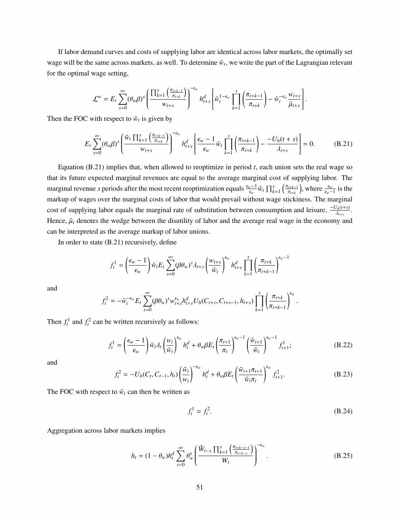
If labor demand curves and costs of supplying labor are identical across labor markets, the optimally set

wage will be the same across markets, as well. To determine wt, we write the part of the Lagrangian relevant

for the optimal wage setting,

Lw = Et

∞∑s=0

(θwβ)s

∏s

k=1

(πt+k−1πt+k

)wt+s

−εw

hdt+s

w1−εwt

s∏k=1

(πt+k−1

πt+k

)− w−εw

twt+s

µt+s

.Then the FOC with respect to wt is given by

Et

∞∑s=0

(θwβ)s

wt∏s

k=1

(πt+k−1πt+k

)wt+s

−εw

hdt+s

εw − 1εw

wt

s∏k=1

(πt+k−1

πt+k

)−−Uh(t + s)

λt+s

= 0. (B.21)

Equation (B.21) implies that, when allowed to reoptimize in period t, each union sets the real wage so

that its future expected marginal revenues are equal to the average marginal cost of supplying labor. The

marginal revenue s periods after the most recent reoptimization equals εw−1εw

wt∏s

k=1

(πt+k−1πt+k

), where εw

εw−1 is the

markup of wages over the marginal costs of labor that would prevail without wage stickiness. The marginal

cost of supplying labor equals the marginal rate of substitution between consumption and leisure, −Uh(t+s)λt+s

.

Hence, µt denotes the wedge between the disutility of labor and the average real wage in the economy and

can be interpreted as the average markup of labor unions.

In order to state (B.21) recursively, define

f 1t =

(εw − 1εw

)wtEt

∞∑s=0

(βθw)sλt+s

(wt+s

wt

)εw

hdt+s

s∏k=1

(πt+k

πt+k−1

)εw−1

and

f 2t = −w−εw

t Et

∞∑s=0

(βθw)swεwt+sh

dt+sUh(Ct+s,Ct+s−1, ht+s)

s∏k=1

(πt+k

πt+k−1

)εw

.

Then f 1t and f 2

t can be written recursively as follows:

f 1t =

(εw − 1εw

)wtλt

(wt

wt

)εw

hdt + θwβEt

(πt+1

πt

)εw−1 (wt+1

wt

)εw−1

f 1t+1; (B.22)

and

f 2t = −Uh(Ct,Ct−1, ht)

(wt

wt

)−εw

hdt + θwβEt

(wt+1πt+1

wtπt

)εw

f 2t+1. (B.23)

The FOC with respect to wt can then be written as

f 1t = f 2

t . (B.24)

Aggregation across labor markets implies

ht = (1 − θw)hdt

∞∑s=0

θsw

Wt−s∏s

k=1

(πt+k−s−1πt+k−s

)Wt

−εw

. (B.25)

51

Defining the measure of wage dispersion as

st ≡ (1 − θw)∞∑

s=0

θsw

Wt−s∏s

k=1

(πt+k−s−1πt+k−s

)Wt

−εw

,

we can rewrite equation (B.25) as

ht = sthdt , (B.26)

where the evolution of wage dispersion over time is given by

st = (1 − θw)(wt

wt

)−εw

+ θw

(wt−1

wt

)−εw(πt

πt−1

)εw

st−1. (B.27)

From the definition of the wage index, Wt ≡

[∫ 10 (Wm

t )1−εwdm]1/(1−εw)

, it follows that the real wage rate,

wt, can be expressed as

w1−εwt = (1 − θw)w1−εw

t + θww1−εwt−1

(πt−1

πt

)1−εw

. (B.28)

Equations (B.22)-(B.28) describe the equilibrium in the labor market.

Appendix B.8. Monetary Policy and Market Clearing

We assume that the central bank sets the nominal interest rate, Rnt , according to the following standard

Taylor rule:Rn

t

Rnss

=

(Rn

t−1

Rnss

)ρ ( πt

πss

)φπ ( Yt

Yss

)φy1−ρ

eνt . (B.29)

Hence, the central bank reacts to deviations of inflation and output from their respective steady-state values

and might smooth interest rates over time with a weight ρ. Unsystematic deviations from the Taylor rule in

(B.29) are captured by a mean-zero i.i.d. random variable, νt.

The model is closed by the economy-wide resource constraint,

Yt = Ct + Cet + Cb

t + It + a (ut) Kt−1 + µG(ωt)Rkt Qt−1Kt−1, (B.30)

where Cet and Cb

t denote the real consumption of entrepreneurial and bank net worth, respectively, a(ut)Kt−1

denotes the real adjustment costs due to capital utilization, and µG(ωt)Rkt Qt−1Kt−1 the aggregate monitoring

costs in period t.

52

Appendix C. Additional Simulation Results

Appendix C.1. Calibration

Table C.1 summarizes the calibration of exogenous shock processes other than monetary policy shocksused for the simulation and computation of theoretical unconditional autocorrelations and cross-correlationwith output in Figure C.1 and Figure 3 in the main text. The calibration of productivity, preference, andinvestment-specific shocks is based on the Maximum Likelihood estimation results in Christensen and Dib(2008), while unanticipated and anticipated risk shocks are calibrated in line with the Bayesian estimationresults in Christiano et al. (2014).

Table C.1: Calibration of Additional Shock Processes.

Shock process Parameter Valueautocorrelation coefficient of total factor productivity ρa 0.7625standard deviation of total factor productivity shocks σa 0.0096autocorrelation coefficient of consumer preferences ρe 0.6165standard deviation of consumer preference shocks σe 0.0073autocorrelation coefficient of investment efficiency ρx 0.6562standard deviation of investment efficiency shocks σx 0.0097autocorrelation coefficient of exogenous process for σω ρσ 0.97standard deviation of unanticipated risk shocks σσ 0.07correlation coefficient of anticipated risk shocks ρξ 0.39standard deviation of anticipated risk shocks σξ 0.028

Appendix C.2. Unconditional Autocorrelations

Figure C.1 plots the unconditional autocorrelation coefficients of selected variables and ratios from the

benchmark New-Keynesian DSGE model with our optimal debt contract and the optimal debt contract in

Bernanke et al. (1999) (BGG) against their empirical counterparts, where both simulated time series and data

are HP-filtered before computing second moments. Figure C.1 illustrates that the autocorrelation patterns

implied by either of the DSGE models is qualitatively and quantitatively in line with those in the data.

Appendix C.3. “Too Low for Too Long”

Inspired by the motivation in Taylor (2007), we conduct an informal test of the “too-low-for-too-long”

hypothesis. According to this hypothesis, a prolonged deviation of monetary policy from what is justified

by economic conditions might lead to excessive risk taking in the financial sector. Note that, in our model,

a transitory deviation from the Taylor rule becomes more persistent, the higher the degree of interest-rate

inertia. In this subsection, we therefore compare the effects of a typical expansionary monetary policy shock

for two different values of the Taylor-rule coefficient on the lagged policy rate, ρ, without modifying the

other parameters of the model.

Figure C.2 illustrates that higher interest-rate inertia and thus a more persistent reduction in the policy

rate, Rnt , implies an increase in both the peak effect and the persistence of the impulse response functions

of the entrepreneurial leverage ratio and default threshold to a monetary easing. Accordingly, the optimal

loosening of bank lending standards, measured by the increase in bank lending relative to borrower collateral

53

Figure C.1: Serial Correlation of Selected Variables and Ratios between Period t and Period t − τ, DSGE Model and Data.

0 5 10

−0.5

0

0.5

1Output

τ0 5 10

−0.5

0

0.5

1Investment

τ0 5 10

−0.5

0

0.5

1Loans/Deposits

τ0 5 10

0

0.5

1Net Income/Bank Equity

τ

0 5 10−0.5

0

0.5

1Collateral Requirements

τ0 5 10

−0.5

0

0.5

1Delinquency Rate

τ0 5 10

−0.5

0

0.5

1Net Interest Margin

τ

DataOur contractBGG contract

Notes: Simulated time series and data are HP-filtered (λ = 1, 600). In the data, output corresponds to log(real GDP per capita),

investment to log(real investment expenditure per capita), loans/deposits to log(loans and leases in bank credit/demand deposits)

at commercial banks, net income/bank equity to Call Reports log(net interest income/total equity capital) for commercial banks in

the U.S., collateral requirements to the net percentage of domestic banks increasing collateral requirements for large and middle-

market firms, delinquency rate to delinquency rate on business loans; all commercial banks, and net interest margin to Call Reports

net interest margin for all U.S. banks.

in our model, and the subsequent increase in the default rate of borrowers becomes more pronounced, when

the nominal policy rate is more inertial. In the current example, an increase in the Taylor-rule coefficient, ρ,

from 0.90 to 0.95 almost doubles the maximum response of the leverage ratio from 3.9 to 7.4 basis points

above its steady-state value of 1.537 and postpones the turning point in the leverage ratio (from above to

below its steady state) by 1 quarter. The effects on the impulse response functions of output, consumption,

and investment are qualitatively the same and of a similar order of magnitude.

54

Figure C.2: Selected Impulse Response Functions to an Expansionary Monetary Policy Shock of 25 Basis Points for ρ = 0.90 andρ = 0.95.

5 10 15 20

−0.4

−0.2

0Policy Rate

ρ=0.90ρ=0.95

5 10 15 20

−0.4

−0.2

0Loan Rate

5 10 15 200

0.02

0.04

0.06Net Interest Margin

5 10 15 200

0.02

0.04

0.06Expected EFP

5 10 15 200

0.5

1Default Threshold

5 10 15 200

2

4

Default Rate

5 10 15 200

0.2

0.4

Leverage Ratio

5 10 15 200

0.5

1Bank Profit Share

5 10 15 200

1

2

Bank Lending

5 10 15 20

−0.8−0.6−0.4−0.2

0

Bank Deposits

5 10 15 20

0

1

2

Net Worth

5 10 15 200

5

10

Bank Net Worth

5 10 15 200

1

2

Output

Quarters5 10 15 20

0

0.5

1

Consumption

Quarters5 10 15 20

0

1

2

Investment

Quarters5 10 15 20

0

1

2

Return on Capital

Quarters

Notes: All impulse response functions are expressed in terms of percentage deviations from steady state, except for the policy rate,

the loan rate, the net interest margin, and the expected EFP, which are expressed in terms of percentage points.

55

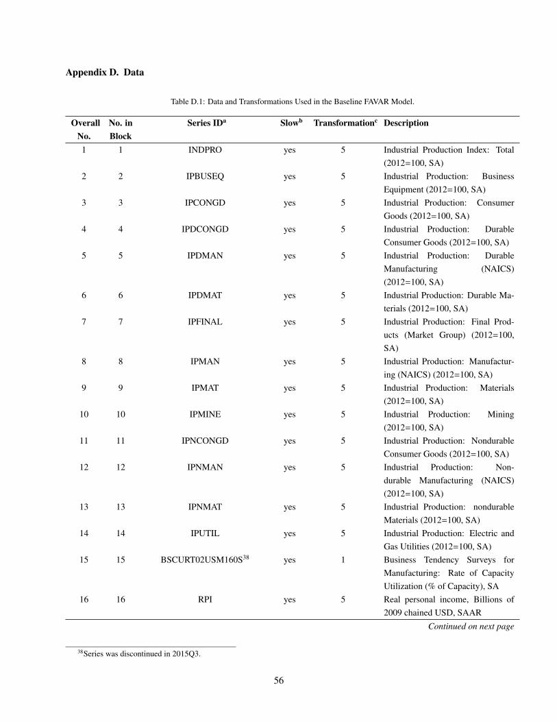
Appendix D. Data

Table D.1: Data and Transformations Used in the Baseline FAVAR Model.

OverallNo.

No. inBlock

Series IDa Slowb Transformationc Description

1 1 INDPRO yes 5 Industrial Production Index: Total(2012=100, SA)

2 2 IPBUSEQ yes 5 Industrial Production: BusinessEquipment (2012=100, SA)

3 3 IPCONGD yes 5 Industrial Production: ConsumerGoods (2012=100, SA)

4 4 IPDCONGD yes 5 Industrial Production: DurableConsumer Goods (2012=100, SA)

5 5 IPDMAN yes 5 Industrial Production: DurableManufacturing (NAICS)(2012=100, SA)

6 6 IPDMAT yes 5 Industrial Production: Durable Ma-terials (2012=100, SA)

7 7 IPFINAL yes 5 Industrial Production: Final Prod-ucts (Market Group) (2012=100,SA)

8 8 IPMAN yes 5 Industrial Production: Manufactur-ing (NAICS) (2012=100, SA)

9 9 IPMAT yes 5 Industrial Production: Materials(2012=100, SA)

10 10 IPMINE yes 5 Industrial Production: Mining(2012=100, SA)

11 11 IPNCONGD yes 5 Industrial Production: NondurableConsumer Goods (2012=100, SA)

12 12 IPNMAN yes 5 Industrial Production: Non-durable Manufacturing (NAICS)(2012=100, SA)

13 13 IPNMAT yes 5 Industrial Production: nondurableMaterials (2012=100, SA)

14 14 IPUTIL yes 5 Industrial Production: Electric andGas Utilities (2012=100, SA)

15 15 BSCURT02USM160S38 yes 1 Business Tendency Surveys forManufacturing: Rate of CapacityUtilization (% of Capacity), SA

16 16 RPI yes 5 Real personal income, Billions of2009 chained USD, SAAR

Continued on next page

38Series was discontinued in 2015Q3.

56

Table D.1 – Continued from previous page

OverallNo.

No. inBlock

Series IDa Slowb Transformationc Description

17 17 W875RX1 yes 5 Real personal income excludingcurrent transfer receipts, Billions of2009 chained USD, SAAR

18 18 GDPC1 yes 5 Real Gross Domestic Product, Bil-lions of 2009 USD chained , SAAR

19 1 CE16OV yes 5 Civilian Employment (thous., SA)20 2 DMANEMP yes 5 All Employees: Durable Goods

(thous., SA)21 3 EMRATIO yes 4 Employment-Population Ratio (Per-

cent, SA)22 4 MANEMP yes 5 All Employees: Manufacturing

(thous., SA)23 5 PAYEMS yes 5 All Employees: Total Nonfarm

(thous., SA)24 6 SRVPRD yes 5 All Employees: Service-Providing

Industries (thous., SA)25 7 USCONS yes 5 All Employees: Construction

(thous., SA)26 8 USGOVT yes 5 All Employees: Government

(thous., SA)27 9 USINFO yes 5 All Employees: Information Ser-

vices (thous., SA)28 10 USMINE yes 5 All Employees: Mining and Log-

ging (thous., SA)29 11 USPRIV yes 5 All Employees: Total Private Indus-

tries (thous., SA)30 12 AWHNONAG yes 1 Average Weekly Hours of Produc-

tion and Nonsupervisory Employ-ees: Total Private (SA)

31 13 CES1000000007 yes 1 Average Weekly Hours of Produc-tion and Nonsupervisory Employ-ees: Mining and Logging (SA)

32 14 CES0800000007 yes 1 Average Weekly Hours of Produc-tion and Nonsupervisory Employ-ees: Private Service Providing, (SA)

33 15 CES3100000007 yes 1 Average Weekly Hours of Produc-tion and Nonsupervisory Employ-ees: Durables (SA)

34 16 CES2000000007 yes 1 Average Weekly Hours of Produc-tion and Nonsupervisory Employ-ees: Construction (SA)

Continued on next page

57

Table D.1 – Continued from previous page

OverallNo.

No. inBlock

Series IDa Slowb Transformationc Description

35 17 CES5000000007 yes 1 Average Weekly Hours of Produc-tion and Nonsupervisory Employ-ees: Information (SA)

36 18 CES4000000007 yes 1 Average Weekly Hours of Produc-tion and Nonsupervisory Employ-ees: Trade, Transportation, Utilities(SA)

37 19 CES6000000007 yes 1 Average Weekly Hours of Produc-tion and Nonsupervisory Employ-ees: Professional and Business Ser-vices (SA)

38 1 PCECC96 yes 5 Real Personal consumption expen-diture, SAAR, chained 2009 BILUSD

39 1 HOUST no 4 Housing Starts: Total: New Pri-vately Owned Housing UnitsStarted (thsd. of units) SAAR

40 2 HOUSTMW no 4 Housing Starts: Midwest: NewPrivately Owned Housing UnitsStarted (thsd. of units) SAAR

41 3 HOUSTNE no 4 Housing Starts: Northeast: NewPrivately Owned Housing UnitsStarted (thsd. of units) SAAR

42 4 HOUSTS no 4 Housing Starts: South: NewPrivately Owned Housing UnitsStarted (thsd. of units) SAAR

43 5 HOUSTW no 4 Housing Starts: West: New Pri-vately Owned Housing UnitsStarted (thsd. of units) SAAR

44 6 PERMIT no 4 New Private Housing Units Autho-rized by Building Permits, (thsd. ofunits) SAAR

45 1 S&P 500 no 5 S&P 500 Stock Price Index, NSA,end of period

46 1 EXCAUS no 5 Canadian Dollars to One U.S. Dol-lar, NSA

47 2 EXJPUS no 5 Japanese Yen to One U.S. Dollar,NSA

48 3 EXSZUS no 5 Swiss Francs to One U.S. Dollar,NSA

Continued on next page

58

Table D.1 – Continued from previous page

OverallNo.

No. inBlock

Series IDa Slowb Transformationc Description

49 4 EXUSUK no 5 U.S. Dollars to One British Pound,NSA

50 1 AAA no 1 Moody’s Seasoned Aaa CorporateBond Yield, Percent, NSA

51 2 BAA no 1 Moody’s Seasoned Baa CorporateBond Yield, Percent, NSA

52 3 FEDFUNDS no 1 Effective FFR, Percent, NSA53 4 GS1 no 1 1-Year Treasury Constant Maturity

Rate, Percent, NSA54 5 GS10 no 1 10-Year Treasury Constant Maturity

Rate, Percent, NSA55 6 GS3 no 1 3-Year Treasury Constant Maturity

Rate, Percent, NSA56 7 GS3M no 1 3-Month Treasury Constant Matu-

rity Rate, Percent, NSA57 8 GS5 no 1 5-Year Treasury Constant Maturity

Rate, Percent, NSA58 9 AAA FFR no 1 Spread: AAA-FFR59 10 BAA FFR no 1 Spread: BAA-FFR60 11 GS1 FFR no 1 Spread: GS1-FFR61 12 GS10 FFR no 1 Spread: GS10-FFR62 13 GS3 FFR no 1 Spread: GS3-FFR63 14 GS3M FFR no 1 Spread: GS3M-FFR64 15 GS5 FFR no 1 Spread:GS5-FFR65 1 BOGNONBR39 no 5 Non-Borrowed Reserves of Deposi-

tory Institutions, Mill USD, SA66 2 AMBSL no 5 Monetary Base, Bill USD, SA67 3 M1 no 5 M1, Bill USD, SA68 4 M2 no 5 M2, Bill USD, SA69 5 MZM no 5 MZM, Bill USD, SA70 6 TOTLL no 5 Total Loans and Leases, Bill USD,

SA71 7 REALLN no 5 Real estate loans, Bill USD, SA72 8 BUSLOANS no 5 C&I loans, Bill USD; SA73 9 CONSUMER no 5 Consumer loans, Bill USD, SA74 1 CPIAUCSL yes 5 Consumer Price Index for All Ur-

ban Consumers: All Items, 1982-84=100, SA

Continued on next page

39Series was discontinued in May 2013.

59

Table D.1 – Continued from previous page

OverallNo.

No. inBlock

Series IDa Slowb Transformationc Description

75 2 CPIFABSL yes 5 Consumer Price Index for All Ur-ban Consumers: Food and Bever-ages, 1982-84=100, SA

76 3 CPILFESL yes 5 Consumer Price Index for All UrbanConsumers: All Items Less Food &Energy, 1982-84=100, SA

77 4 CPIMEDSL yes 5 Consumer Price Index for All UrbanConsumers: Medical Care, 1982-84=100, SA

78 5 DNRGRG3M086SBEA yes 5 Personal consumption expenditures:Energy goods and services, chain-type index, 2009=100

79 6 DPCXRG3M086SBEA yes 5 Personal consumption expendi-tures: Market-based PCE excludingfood and energy, chain-type index,2009=100

80 7 PPICRM no 5 Producer Price Index: CrudeMaterials for Further Processing,1982=100, SA

81 8 PPIFCG yes 5 Producer Price Index: FinishedConsumer Goods, 1982=100, SA

82 9 PPIFGS yes 5 Producer Price Index: FinishedGoods, 1982=100, SA

83 10 PPIIEG yes 5 Producer Price Index: IntermediateEnergy Goods, 1982=100, SA

84 11 PPIITM yes 5 Producer Price Index: IntermediateMaterials: Supplies & Components,1982=100, SA

85 1 CSCICP02USM661S40 no 1 Consumer Opinion Surveys: Confi-dence Indicators: Composite Indi-cator, 2005=1.00, SA, end of period

86 1 SUBLPDCILS N.Q no 1 Net percentage of domestic bankstightening standards for C&I loansto large and middle-market firms,Percentage

Continued on next page

40Series was discontinued in 2013Q2.

60

Table D.1 – Continued from previous page

OverallNo.

No. inBlock

Series IDa Slowb Transformationc Description

87 2 SUBLPDCILTC N.Q no 1 Net percentage of domestic banksincreasing the cost of credit lines tolarge and middle-market firms, Per-centage

88 3 SUBLPDCILTL N.Q no 1 Net percentage of domestic bankstightening loan covenants for largeand middle-market firms, Percent-age

89 4 SUBLPDCILTM N.Q no 1 Net percentage of domestic banksreducing the maximum size ofcredit lines for large and middle-market firms, Percentage

90 5 SUBLPDCILTQ N.Q no 1 Net percentage of domestic banksincreasing collateral requirementsfor large and middle-market firms,Percentage

91 6 SUBLPDCILTS N.Q no 1 Net percentage of domestic banksincreasing spreads of loan rates overbanks’ cost of funds to large andmiddle-market firms, Percentage

92 7 SUBLPDCISS N.Q no 1 Net percentage of domestic bankstightening standards for C&I loansto small firms, Percentage

93 8 SUBLPDCISTC N.Q no 1 Net percentage of domestic banksincreasing the cost of credit lines tosmall firms, Percentage

94 9 SUBLPDCISTL N.Q no 1 Net percentage of domestic bankstightening loan covenants for smallfirms, Percentage

95 10 SUBLPDCISTM N.Q no 1 Net percentage of domestic banksreducing the maximum size creditlines for small firms, Percentage

96 11 SUBLPDCISTQ N.Q no 1 Net percentage of domestic banksincreasing collateral requirementsfor small firms, Percentage

97 12 SUBLPDCISTS N.Q no 1 Net percentage of domestic banksincreasing spreads of loan rates overbanks’ cost of funds to small firms,Percentage

Continued on next page

61

Table D.1 – Continued from previous page

OverallNo.

No. inBlock

Series IDa Slowb Transformationc Description

98 13 SUBLPDRCS N.Q no 1 Net percentage of domestic bankstightening standards for commercialreal estate loans, Percentage

99 14 SUBLPFCIS N.Q no 1 Net percentage of foreign bankstightening standards for approvingC&I loans, Percentage

100 15 SUBLPFCITC N.Q no 1 Net percentage of foreign banks in-creasing costs of credit lines, Per-centage

101 16 SUBLPFCITL N.Q no 1 Net percentage of foreign bankstightening loan covenants, Percent-age

102 17 SUBLPFCITM N.Q no 1 Net percentage of foreign banks re-ducing the maximum size of creditlines, Percentage

103 18 SUBLPFCITQ N.Q no 1 Net percentage of foreign banksincreasing collateralization require-ments, Percentage

104 19 SUBLPFRCS N.Q no 1 Net percentage of foreign bankstightening standards for commercialreal estate loans, Percentage

105 1 AHETPI yes 5 Average Hourly Earnings of Pro-duction and Nonsupervisory Em-ployees: Total Private, USD perHour, SA

106 2 CES0600000008 yes 5 Average Hourly Earnings of Pro-duction and Nonsupervisory Em-ployees: Goods producing, USDper hour, SA

107 3 CES0800000008 yes 5 Average Hourly Earnings of Pro-duction and Nonsupervisory Em-ployees: Private Service Producing,USD per Hour, SA

108 4 CES1000000008 yes 5 Average Hourly Earnings of Pro-duction and Nonsupervisory Em-ployees: Mining and Logging, USDper Hour, SA

109 5 CES2000000008 yes 5 Average Hourly Earnings of Pro-duction and Nonsupervisory Em-ployees: Construction, USD perHour, SA

Continued on next page

62

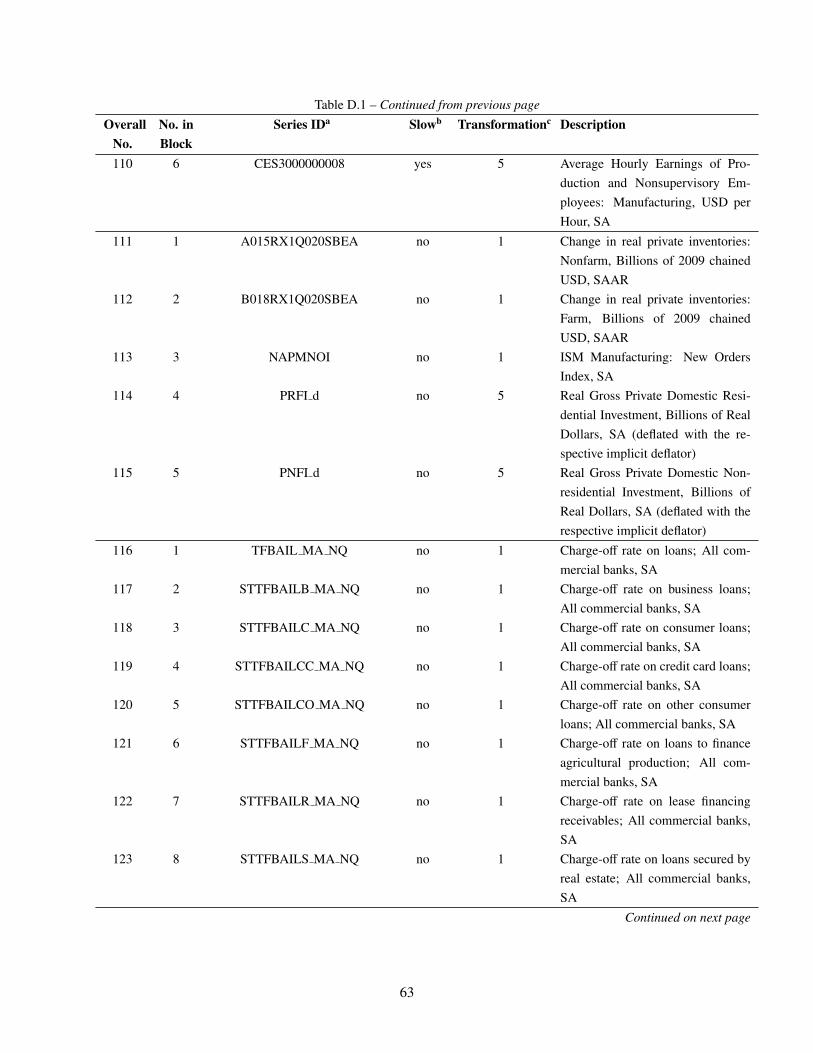
Table D.1 – Continued from previous page

OverallNo.

No. inBlock

Series IDa Slowb Transformationc Description

110 6 CES3000000008 yes 5 Average Hourly Earnings of Pro-duction and Nonsupervisory Em-ployees: Manufacturing, USD perHour, SA

111 1 A015RX1Q020SBEA no 1 Change in real private inventories:Nonfarm, Billions of 2009 chainedUSD, SAAR

112 2 B018RX1Q020SBEA no 1 Change in real private inventories:Farm, Billions of 2009 chainedUSD, SAAR

113 3 NAPMNOI no 1 ISM Manufacturing: New OrdersIndex, SA

114 4 PRFI d no 5 Real Gross Private Domestic Resi-dential Investment, Billions of RealDollars, SA (deflated with the re-spective implicit deflator)

115 5 PNFI d no 5 Real Gross Private Domestic Non-residential Investment, Billions ofReal Dollars, SA (deflated with therespective implicit deflator)

116 1 TFBAIL MA NQ no 1 Charge-off rate on loans; All com-mercial banks, SA

117 2 STTFBAILB MA NQ no 1 Charge-off rate on business loans;All commercial banks, SA

118 3 STTFBAILC MA NQ no 1 Charge-off rate on consumer loans;All commercial banks, SA

119 4 STTFBAILCC MA NQ no 1 Charge-off rate on credit card loans;All commercial banks, SA

120 5 STTFBAILCO MA NQ no 1 Charge-off rate on other consumerloans; All commercial banks, SA

121 6 STTFBAILF MA NQ no 1 Charge-off rate on loans to financeagricultural production; All com-mercial banks, SA

122 7 STTFBAILR MA NQ no 1 Charge-off rate on lease financingreceivables; All commercial banks,SA

123 8 STTFBAILS MA NQ no 1 Charge-off rate on loans secured byreal estate; All commercial banks,SA

Continued on next page

63

Table D.1 – Continued from previous page

OverallNo.

No. inBlock

Series IDa Slowb Transformationc Description

124 9 STTFBAILSF XDO MA NQ no 1 Charge-off rate on farmland loans,booked in domestic offices; Allcommercial banks, SA

125 10 STTFBAILSS XDO MA NQ no 1 Charge-off rate on single familyresidential mortgages, booked indomestics offices; All commercialbanks, SA

126 11 STTFBAILSX XDO MA NQ no 1 Charge-off rate on commercial realestate loans (excluding farmland),booked in domestic offfices; Allcommercial banks, SA

127 12 STTFBAIL XEOP MA NQ no 1 Delinquency rate on loans; All com-mercial banks, SA

128 13 STTFBAILB XEOP MA NQ no 1 Delinquency rate on business loans;All commercial banks, SA

129 14 STTFBAILC XEOP MA NQ no 1 Delinquency rate on consumerloans; All commercial banks, SA

130 15 STTFBAILCC XEOP MA NQ no 1 Delinquency rate on credit cardloans; All commercial banks, SA

131 16 STTFBAILCO XEOP MA NQ no 1 Delinquency rate on other consumerloans; All commercial banks, SA

132 17 STTFBAILF XEOP MA NQ no 1 Delinquency rate on loans to financeagricultural production; All com-mercial banks, SA

133 18 STTFBAILR XEOP MA NQ no 1 Delinquency rate on lease financingreceivables; All commercial banks,SA

134 19 STTFBAILS XEOP MA NQ no 1 Delinquency rate on loans securedby real estate; All commercialbanks, SA

135 20 STTFBAILSF XEOP XDO MA NQ no 1 Delinquency rate on farmland loans,booked in domestic offices; Allcommercial banks, SA

136 21 STTFBAILSS XEOP XDO MA NQ no 1 Delinquency rate on single-familyresidential mortgages, booked indomestic offices; All commercialbanks, SA

Continued on next page

64

Table D.1 – Continued from previous page

OverallNo.

No. inBlock

Series IDa Slowb Transformationc Description

137 22 STTFBAILSX XEOP XDO MA NQ no 1 Delinquency rate on commercialreal estate loans (excluding farm-land), booked in domestic offices;All commercial banks, SA

138 1 BANKPROFIT no 5 BEA Profits of Other Financial In-stitutions, Billions of USD, SAAR

139 2 FEDPROFIT no 5 BEA Profits of Federal ReserveBanks, Billions of USD, SAAR

140 3 CALLNETINCOME no 5 Net Income for Commercial Banks,Thous. USD, NSA, adjusted for cu-mulative accounting

141 4 CALLNETINTINCOME no 5 Net Interest Income for CommercialBanks, Thous. USD, NSA, adjustedfor cumulative accounting

142 5 CALLNETMARGIN no 1 Net Interest Margin for US Banks,Percent, End of Period, NSA

a Macroeconomic time series are taken from the FRED database, lending standards measures are taken from theSenior Loan Officer Opinion Survey (SLOOS) of the Federal Reserve.

b If yes, a variable is assumed to be slow-moving when estimated with a principal component approach.c Variable transformations codes are as follows: 1 - no transformation, 2 - difference, 4 - logarithm, 5 - log-difference.

65

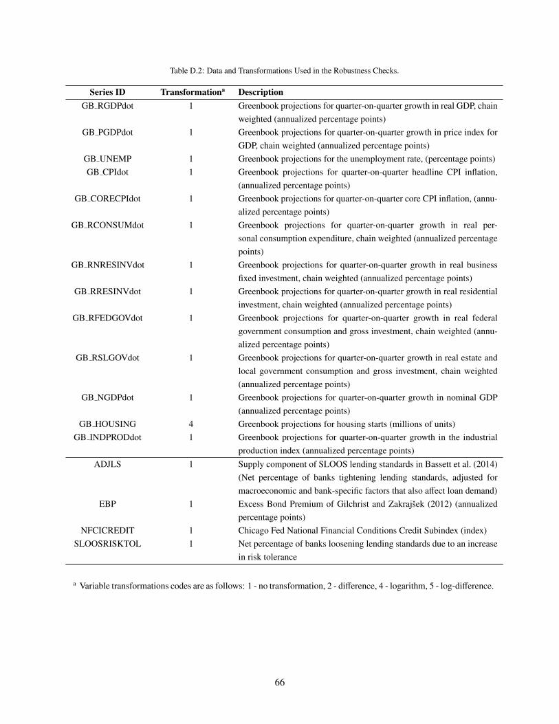
Table D.2: Data and Transformations Used in the Robustness Checks.

Series ID Transformationa DescriptionGB RGDPdot 1 Greenbook projections for quarter-on-quarter growth in real GDP, chain

weighted (annualized percentage points)GB PGDPdot 1 Greenbook projections for quarter-on-quarter growth in price index for

GDP, chain weighted (annualized percentage points)GB UNEMP 1 Greenbook projections for the unemployment rate, (percentage points)GB CPIdot 1 Greenbook projections for quarter-on-quarter headline CPI inflation,

(annualized percentage points)GB CORECPIdot 1 Greenbook projections for quarter-on-quarter core CPI inflation, (annu-

alized percentage points)GB RCONSUMdot 1 Greenbook projections for quarter-on-quarter growth in real per-

sonal consumption expenditure, chain weighted (annualized percentagepoints)

GB RNRESINVdot 1 Greenbook projections for quarter-on-quarter growth in real businessfixed investment, chain weighted (annualized percentage points)

GB RRESINVdot 1 Greenbook projections for quarter-on-quarter growth in real residentialinvestment, chain weighted (annualized percentage points)

GB RFEDGOVdot 1 Greenbook projections for quarter-on-quarter growth in real federalgovernment consumption and gross investment, chain weighted (annu-alized percentage points)

GB RSLGOVdot 1 Greenbook projections for quarter-on-quarter growth in real estate andlocal government consumption and gross investment, chain weighted(annualized percentage points)

GB NGDPdot 1 Greenbook projections for quarter-on-quarter growth in nominal GDP(annualized percentage points)

GB HOUSING 4 Greenbook projections for housing starts (millions of units)GB INDPRODdot 1 Greenbook projections for quarter-on-quarter growth in the industrial

production index (annualized percentage points)ADJLS 1 Supply component of SLOOS lending standards in Bassett et al. (2014)

(Net percentage of banks tightening lending standards, adjusted formacroeconomic and bank-specific factors that also affect loan demand)

EBP 1 Excess Bond Premium of Gilchrist and Zakrajsek (2012) (annualizedpercentage points)

NFCICREDIT 1 Chicago Fed National Financial Conditions Credit Subindex (index)SLOOSRISKTOL 1 Net percentage of banks loosening lending standards due to an increase

in risk tolerance

a Variable transformations codes are as follows: 1 - no transformation, 2 - difference, 4 - logarithm, 5 - log-difference.

66

Appendix E. Bayesian Estimation of the FAVAR Model

In order to jointly estimate equations (19) and (20) using Bayesian methods it is convenient to rewrite

the model in state-space form: Xt

Yt

=

Λ f Λy

0 I

Ft

Yt

+

et

0

(E.1)

Ft

Yt

= Φ (L)

Ft−1

Yt−1

+ νt, (E.2)

where Yt is the M × 1 vector of observables, Ft is the K × 1 vector of unobservable factors, and Xt is the

N × 1 vector of informational time series. We restrict the loading coefficient matrices Λ f of dimension

N × K and Λy of dimension N × M in order to identify the factors uniquely. The vector error terms et and

νt are assumed to be normally distributed and uncorrelated, i.e. et ∼ N (0,R) and νt ∼ N (0,Q), where R is a

diagonal matrix.

In one-step Bayesian estimation, all parameters are treated as random variables. The parameter vector

θ contains the factor loadings and the variance-covariance matrix of the observation equation in (19) as

well as the VAR coefficients and the variance-covariance matrix of the transition equation in (20) , i.e., θ =(Λ f ,Λy,R, vec (Φ) ,Q

). In addition, the unobservable factors are treated as random variables and sampled.

The observation and transition equations can be rewritten as

Xt = ΛFt + et (E.3)

Ft = Φ (L) Ft−1 + νt, (E.4)

where Λ is the loading matrix, Xt =(X′t ,Y

′t), et =

(e′t , 0

), and Ft =

(F′t ,Y

′t). Let Xt = (X1, X2, . . . , XT ) and

Ft = (F1, F2, . . . , FT ) denote the respective histories from time 1 to T . Our goal is to obtain the marginal

densities of the parameters and factors, which can be integrated out of the joint posterior density p(θ, FT

).

Hence, we are interested in the following objects:

p(FT

)=

∫p(θ, FT

)dθ, (E.5)

p (θ) =

∫p(θ, FT

)dFT . (E.6)

Appendix E.1. The Gibbs Sampler

We use the multi-move Gibbs sampling approach of Carter and Kohn (1994), which alternately samples

from the parameters and the factors as follows:

1. Choose a starting value for the parameter vector θ0.

2. Draw F(1)T from the conditional density p

(FT |XT , θ0

).

3. Draw θ(1) from the conditional density p(θ|XT , F

(1)T

).

Repeat steps 2 and 3 until convergence.

67

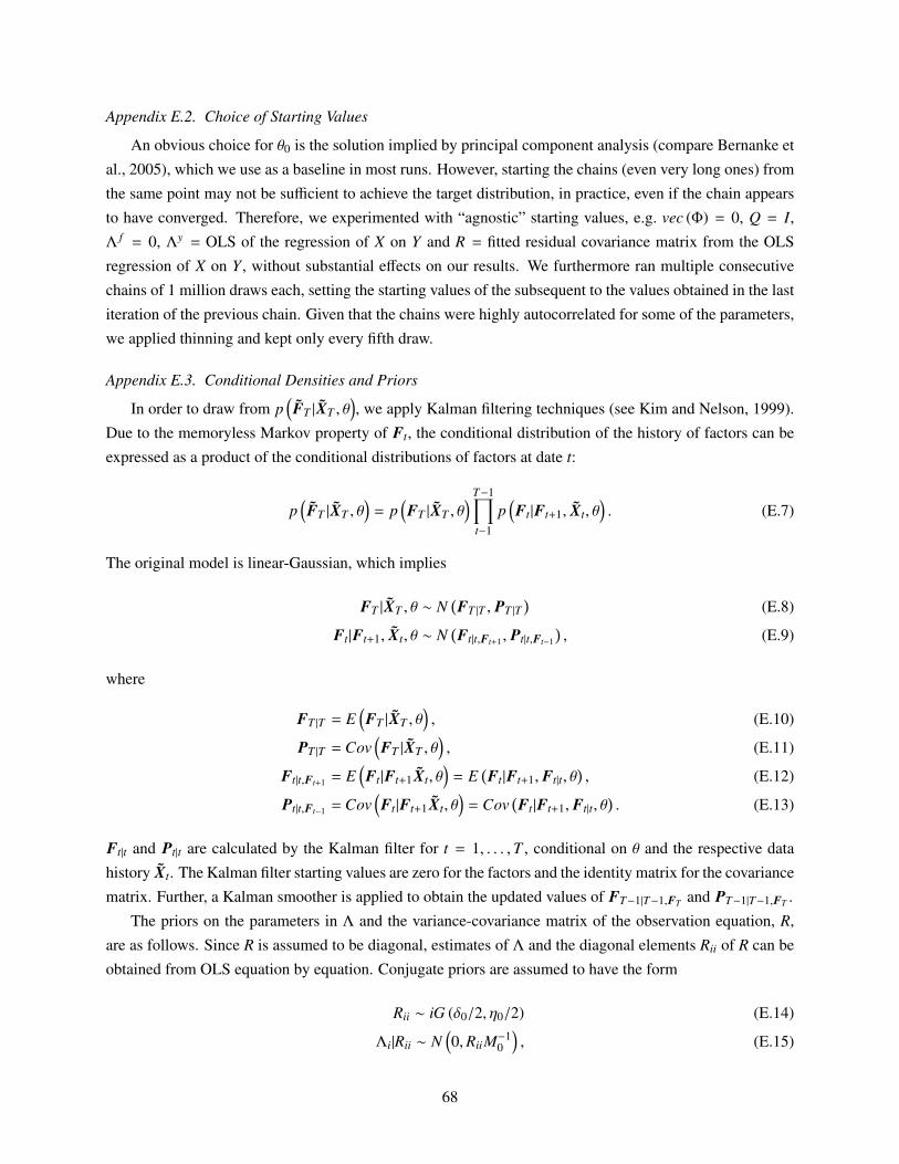
Appendix E.2. Choice of Starting Values

An obvious choice for θ0 is the solution implied by principal component analysis (compare Bernanke et

al., 2005), which we use as a baseline in most runs. However, starting the chains (even very long ones) from

the same point may not be sufficient to achieve the target distribution, in practice, even if the chain appears

to have converged. Therefore, we experimented with “agnostic” starting values, e.g. vec (Φ) = 0, Q = I,

Λ f = 0, Λy = OLS of the regression of X on Y and R = fitted residual covariance matrix from the OLS

regression of X on Y , without substantial effects on our results. We furthermore ran multiple consecutive

chains of 1 million draws each, setting the starting values of the subsequent to the values obtained in the last

iteration of the previous chain. Given that the chains were highly autocorrelated for some of the parameters,

we applied thinning and kept only every fifth draw.

Appendix E.3. Conditional Densities and Priors

In order to draw from p(FT |XT , θ

), we apply Kalman filtering techniques (see Kim and Nelson, 1999).

Due to the memoryless Markov property of Ft, the conditional distribution of the history of factors can be

expressed as a product of the conditional distributions of factors at date t:

p(FT |XT , θ

)= p

(FT |XT , θ

) T−1∏t−1

p(Ft|Ft+1, Xt, θ

). (E.7)

The original model is linear-Gaussian, which implies

FT |XT , θ ∼ N(FT |T , PT |T

)(E.8)

Ft|Ft+1, Xt, θ ∼ N(Ft|t,Ft+1 , Pt|t,Ft−1

), (E.9)

where

FT |T = E(FT |XT , θ

), (E.10)

PT |T = Cov(FT |XT , θ

), (E.11)

Ft|t,Ft+1 = E(Ft|Ft+1Xt, θ

)= E

(Ft|Ft+1, Ft|t, θ

), (E.12)

Pt|t,Ft−1 = Cov(Ft|Ft+1Xt, θ

)= Cov

(Ft|Ft+1, Ft|t, θ

). (E.13)

Ft|t and Pt|t are calculated by the Kalman filter for t = 1, . . . ,T , conditional on θ and the respective data

history Xt. The Kalman filter starting values are zero for the factors and the identity matrix for the covariance

matrix. Further, a Kalman smoother is applied to obtain the updated values of FT−1|T−1,FT and PT−1|T−1,FT .

The priors on the parameters in Λ and the variance-covariance matrix of the observation equation, R,

are as follows. Since R is assumed to be diagonal, estimates of Λ and the diagonal elements Rii of R can be

obtained from OLS equation by equation. Conjugate priors are assumed to have the form

Rii ∼ iG (δ0/2, η0/2) (E.14)

Λi|Rii ∼ N(0,RiiM−1

0

), (E.15)

68

where, following Bernanke et al. (2005), we set δ0 = 6, η0 = 2 · 10−3 and M0 = I. Given the above priors, it

can be shown that the corresponding posterior distributions have the form

Rii|XT , FT ∼ iG (δi/2, η/2) (E.16)

Λi|Rii, XT , FT ∼ N(Λi,RiiM−1

i

), (E.17)

where

δi = δ0/2 + e′i ei + Λ′i

[M−1

0 +

(F′iT Fi

T

)−1]−1

Λi, (E.18)

η = η0/2 + T, (E.19)

Λi = M−1i

(F′iT Fi

T

)Λi, (E.20)

Mi = M0 + F′iT FiT , (E.21)

and FiT are the regressors of the ith equation.

The priors on the transition (state) equation are as follows. As the transition equation corresponds to

a standard VAR, it can be estimated by OLS equation by equation to obtain vec(Φ)

and Q. We impose a

conjugate Normal-Inverse-Wishart prior,

Q ∼ iW (Q0,K + M + 2) (E.22)

vec (Φ) |Q ∼ N (0,Q ⊗Ω0) , (E.23)

where the diagonal elements of Q0 are set to the residual variances of the corresponding univariate regres-

sions, σ2i , as in Kadiyala and Karlsson (1997). The diagonal elements of Ω0 are set in the spirit of the

Minnesota prior, i.e. the prior variance of the coefficient on variable j at lag k in equation i is σ2i /kσ

2j . This

prior yields the following conjugate posterior:

Q|XT , FT ∼ iW(Q,T + K + M + 2

)(E.24)

vec (Φ) |Q, XT , FT ∼ N(vec

(Φ),Q ⊗ Ω

), (E.25)

where

Q = Q0 + V ′V + Φ′[Ω0 +

(F′T−1FT−1

)−1]−1

Φ (E.26)

Φ = Ω(F′T−1FT−1

)Φ (E.27)

Ω =(Ω−1

0 + F′T−1FT−1)−1

(E.28)

and V is the matrix of OLS residuals.

Following Bernanke et al. (2005) and Amir Ahmadi and Uhlig (2009), we enforce stationarity by trun-

cating draws of Φ where the largest eigenvalue exceeds 1 in absolute value.

69

Appendix E.4. Monitoring Convergence

Geman and Geman (1984) show that both joint and marginal distributions will converge to their target

distributions at an exponential rate as the number of replications approaches infinity. In practice, however,

the Gibbs sampler may converge slowly and requires careful monitoring. We monitor convergence by (i)

plotting the coefficients against the number of replications (level shifts and trends should not occur); (ii)

comparing the medians and means of the coefficients at different parts of the chain (large differences should

not occur); (iii) plotting and comparing the medians of the factors obtained from first and second half of the

chain (large and frequent deviations should not occur). The corresponding figures for our baseline model

with 3 factors are reported below. It turns out that convergence is quite slow and becomes increasingly

difficult to achieve, if we increase the number of unobserved factors.

Appendix E.5. Normalization of Unobserved Factors

Due to the fundamental indeterminacy of factor models, the unobserved factors can only be estimated

up to a rotation. For this reason, we must impose a set of standard restrictions on the observation equation in

order to identify the factors uniquely. Following Bernanke et al. (2005), we eliminate rotations of the form

F∗t = AFt + BYt. Solving this expression for Ft and plugging the result into the observation equation in (19)

yields

Xt = Λ f A−1F∗t + (Λy + Λ f A−1B)Yt. (E.29)

Hence, the unique identification of factors requires that A−1F∗t = Ft and Λ f A−1B = 0. Bernanke et al. (2005)

suggest imposing sufficient (overidentifying) restrictions by setting A = I and B = 0. Moreover, the one-

step estimation approach requires that the first K variables in the vector Xt belong to the set of slow-moving

variables (compare Table D.1).

70

Figure E.1: Monitoring of Factor Convergence and Factor Uncertainty for the Baseline FAVAR Model.

1991Q1 1994Q1 1997Q1 2000Q1 2003Q1 2006Q1−2

−1.5

−1

−0.5

0

0.5

1

1.5

2

Median First HalfMedian Second Half

(a) Factor 1: Median of first & second half of draws post burn-in.

1991Q1 1994Q1 1997Q1 2000Q1 2003Q1 2006Q1−2

−1.5

−1

−0.5

0

0.5

1

1.5

2

5%−PercentileMedian95%−Percentile

(b) Factor 1: Median of all draws after burn-in & 90% coverage.

1991Q1 1994Q1 1997Q1 2000Q1 2003Q1 2006Q1−2.5

−2

−1.5

−1

−0.5

0

0.5

1

1.5

Median First HalfMedian Second Half

(c) Factor 2: Median of first & second half of draws post burn-in.

1991Q1 1994Q1 1997Q1 2000Q1 2003Q1 2006Q1−2.5

−2

−1.5

−1

−0.5

0

0.5

1

1.5

5%−PercentileMedian95%−Percentile

(d) Factor 2: Median of all draws after burn-in & 90% coverage.

1991Q1 1994Q1 1997Q1 2000Q1 2003Q1 2006Q1−0.8

−0.6

−0.4

−0.2

0

0.2

0.4

0.6

0.8

1

Median First HalfMedian Second Half

(e) Factor 3: Median of first & second half of draws post burn-in.

1991Q1 1994Q1 1997Q1 2000Q1 2003Q1 2006Q1−0.8

−0.6

−0.4

−0.2

0

0.2

0.4

0.6

0.8

1

5%−PercentileMedian95%−Percentile

(f) Factor 3: Median of all draws after burn-in & 90% coverage.

71

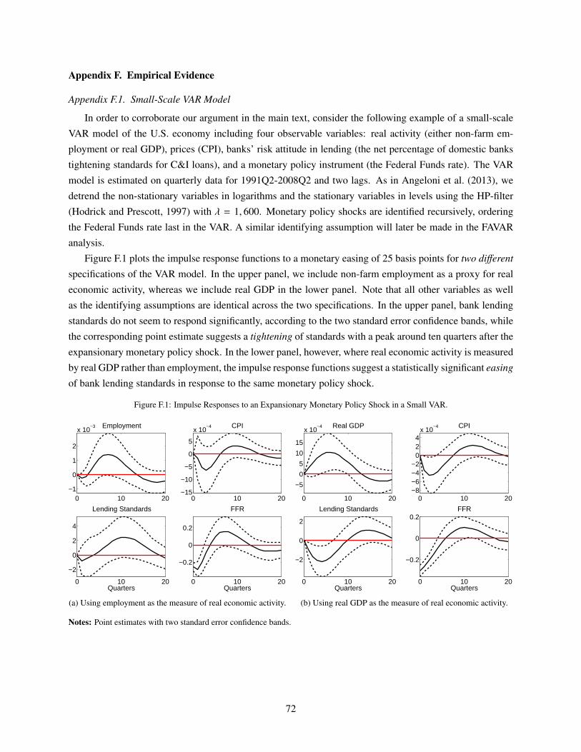
Appendix F. Empirical Evidence

Appendix F.1. Small-Scale VAR Model

In order to corroborate our argument in the main text, consider the following example of a small-scale

VAR model of the U.S. economy including four observable variables: real activity (either non-farm em-

ployment or real GDP), prices (CPI), banks’ risk attitude in lending (the net percentage of domestic banks

tightening standards for C&I loans), and a monetary policy instrument (the Federal Funds rate). The VAR

model is estimated on quarterly data for 1991Q2-2008Q2 and two lags. As in Angeloni et al. (2013), we

detrend the non-stationary variables in logarithms and the stationary variables in levels using the HP-filter

(Hodrick and Prescott, 1997) with λ = 1, 600. Monetary policy shocks are identified recursively, ordering

the Federal Funds rate last in the VAR. A similar identifying assumption will later be made in the FAVAR

analysis.

Figure F.1 plots the impulse response functions to a monetary easing of 25 basis points for two different

specifications of the VAR model. In the upper panel, we include non-farm employment as a proxy for real

economic activity, whereas we include real GDP in the lower panel. Note that all other variables as well

as the identifying assumptions are identical across the two specifications. In the upper panel, bank lending

standards do not seem to respond significantly, according to the two standard error confidence bands, while

the corresponding point estimate suggests a tightening of standards with a peak around ten quarters after the

expansionary monetary policy shock. In the lower panel, however, where real economic activity is measured

by real GDP rather than employment, the impulse response functions suggest a statistically significant easing

of bank lending standards in response to the same monetary policy shock.

Figure F.1: Impulse Responses to an Expansionary Monetary Policy Shock in a Small VAR.

0 10 20−1

0

1

2

x 10−3 Employment

0 10 20−15

−10

−5

0

5

x 10−4 CPI

0 10 20

−2

0

2

4

Lending Standards

Quarters0 10 20

−0.2

0

0.2

FFR

Quarters

(a) Using employment as the measure of real economic activity.

0 10 20

−5

0

5

10

15

x 10−4 Real GDP

0 10 20−8−6−4−2

024

x 10−4 CPI

0 10 20

−2

0

2

Lending Standards

Quarters0 10 20

−0.2

0

0.2FFR

Quarters

(b) Using real GDP as the measure of real economic activity.

Notes: Point estimates with two standard error confidence bands.

72

Appendix F.2. Explanatory Power of Latent Factors

Given that our main interest is in explaining the fluctuations in lending standards, Table F.1 reports the

median adjusted R2 for each of the 19 SLOOS measures based on the FAVAR model with one, three, five,

and seven unobservable factors. We find that the first factor exhibits a high correlation with most measures of

bank lending standards. The respective adjusted R2 ranges from .148 for foreign banks tightening standards

for commercial real estate loans to .882 for domestic banks increasing the cost of credit lines to large and

middle firms. With very few exceptions, adding further factors improves this tight fit only marginally.

Table F.1: Adjusted R2 for SLOOS Measures of Lending Standards, 1991Q1-2008Q2.

No. Lending Standard Description 1 factor 3 factors 5 factors 7 factors1 domestic banks tightening standards on C&I loans

to large and middle firms0.880 0.890 0.905 0.907

2 domestic banks increasing the costs of credit linesto large and middle firms

0.882 0.867 0.862 0.857

3 domestic banks tightening loan covenants forlarge and middle firms

0.877 0.909 0.914 0.922

4 domestic banks reducing the maximum size ofcredit lines to large and middle firms

0.870 0.879 0.885 0.885

5 domestic banks increasing collateral requirementsfor large and middle firms

0.523 0.603 0.613 0.614

6 domestic banks increasing spreads of loan ratesover banks’ cost of funds to large and middle firms

0.875 0.849 0.848 0.830

7 domestic banks tightening standards for C&Iloans to small firms

0.774 0.804 0.839 0.843

8 domestic banks increasing the cost of credit linesto small firms

0.800 0.800 0.843 0.842

9 domestic banks tightening loan covenants forsmall firms

0.811 0.826 0.840 0.840

10 domestic banks reducing the maximum size ofcredit lines to small firms

0.734 0.713 0.747 0.732

11 domestic banks increasing collateral requirementsfor small firms

0.270 0.362 0.420 0.397

12 domestic banks increasing spreads of loan ratesover banks’ cost of funds to small firms

0.830 0.844 0.875 0.867

13 domestic banks tightening standards for commer-cial real estate loans

0.467 0.597 0.718 0.725

14 foreign banks tightening standards for approvingC&I loans

0.728 0.784 0.789 0.803

15 foreign banks increasing costs of credit lines 0.719 0.730 0.759 0.78016 foreign banks tightening loan covenants 0.759 0.784 0.785 0.79817 foreign banks reducing the maximum size of

credit lines0.584 0.638 0.633 0.682

18 foreign banks increasing collateral requirements 0.430 0.511 0.493 0.50319 foreign banks tightening standards for commercial

real estate loans0.148 0.204 0.190 0.230

Notes: Median adjusted R2 based on last 10,000 draws from the Gibbs sampler for the baseline FAVAR model with one, three, five,

and seven unobserved factors.

73

Appendix F.3. Historical Variance Decomposition

We are primarily interested in the response of the 19 measures of bank lending standards to expansionary

monetary policy shocks, on average over the sample period. In order to assess the plausibility of our FAVAR

specification and the resulting monetary shock series, we consider the historical variance decomposition

(HVD) of the standardized changes in lending standards. Figure F.2 plots the cumulative contributions of

monetary policy shocks to fluctuations in the Federal Funds rate and lending standards for a single candidate

draw from the Gibbs sampler, after discarding a sufficiently long burn-in phase.41

Over the second half of the sample, we find that unexpected monetary policy shocks contribute to the

reduction in the Federal Funds rate after the dot-com bubble and, to a lesser extent, to the gradual change

in the monetary policy stance during the boom preceding the Great Recession.42 Moreover, the FAVAR

model attributes a sizeable share of the initial tightening and subsequent loosening of bank lending standards

between 1998 and 2005 to monetary shocks. Note that this HVD pattern is shared by all 19 measures. In

line with conventional wisdom, the abrupt tightening of lending standards in 2008 is not associated with

unexpected monetary policy shocks.

Appendix F.4. Impulse Response Functions of SLOOS Lending Standards

Appendix G. Robustness of Empirical Evidence

Appendix G.1. Number of Latent Factors

41The reason for plotting the HVD based on a single model is that pointwise median contributions based on all draws implyjumping between different candidates and are thus not interpretable in a sensible way. Nevertheless, the latter results are qualitativelyand quantitatively very similar to those in Figure F.2, which can therefore be considered as representative.

42It is well-known that HVD contributions go through a transition phase that can be protracted if the time series in question areserially correlated. Here, the transition phase lasts until roughly 1998 and our discussion therefore focuses on the results thereafter.

74

Figu

reF.

2:C

ontr

ibut

ion

ofM

onet

ary

Polic

ySh

ocks

toH

isto

rica

lVar

ianc

eD

ecom

posi

tion

ofFF

Ran

dL

endi

ngSt

anda

rds

inth

eFA

VAR

Mod

elw

ithT

hree

Uno

bser

ved

Fact

ors

for

1991

Q1-

2008

Q2.

1995

2000

2005

−202

Fed

eral

Fun

ds R

ate

Dat

aH

VD

1995

2000

2005

−2002040

Lend

ing

Sta

ndar

d 1

1995

2000

2005

−40

−200204060

Lend

ing

Sta

ndar

d 2

1995

2000

2005

−2002040

Lend

ing

Sta

ndar

d 3

1995

2000

2005

−2002040

Lend

ing

Sta

ndar

d 4

1995

2000

2005

−2002040

Lend

ing

Sta

ndar

d 5

1995

2000

2005

−50050

Lend

ing

Sta

ndar

d 6

1995

2000

2005

−2002040

Lend

ing

Sta

ndar

d 7

1995

2000

2005

−2002040

Lend

ing

Sta

ndar

d 8

1995

2000

2005

−20020

Lend

ing

Sta

ndar

d 9

1995

2000

2005

−1001020

Lend

ing

Sta

ndar

d 10

1995

2000

2005

−100102030

Lend

ing

Sta

ndar

d 11

1995

2000

2005

−40

−200204060

Lend

ing

Sta

ndar

d 12

1995

2000

2005

−200204060

Lend

ing

Sta

ndar

d 13

1995

2000

2005

−50050

Lend

ing

Sta

ndar

d 14

1995

2000

2005

−50050

Lend

ing

Sta

ndar

d 15

1995

2000

2005

−50050

Lend

ing

Sta

ndar

d 16

1995

2000

2005

−50050

Lend

ing

Sta

ndar

d 17

1995

2000

2005

−20020

Lend

ing

Sta

ndar

d 18

1995

2000

2005

−2002040

Lend

ing

Sta

ndar

d 19

Not

es:P

oint

estim

ates

fora

sing

leca

ndid

ate

draw

from

the

Gib

bssa

mpl

er.S

eeA

ppen

dix

Dfo

rade

taile

dde

scri

ptio

nof

lend

ing

stan

dard

mea

sure

s.

75

Figu

reF.

3:Im

puls

eR

espo

nses

ofL

endi

ngSt

anda

rdM

easu

res

toa

25bp

sE

xpan

sion

ary

Mon

etar

yPo

licy

Shoc

kin

the

Bas

elin

eFA

VAR

Mod

elw

ithT

hree

Uno

bser

ved

Fact

ors

for

1991

Q1-

2008

Q2.

020

−0.

50

0.5

Fed

eral

Fun

ds R

ate

020

−0.

50

0.5

Lend

ing

Sta

ndar

d 1

020

−0.

50

0.5

Lend

ing

Sta

ndar

d 2

020

−0.

50

0.5

Lend

ing

Sta

ndar

d 3

020

−0.

50

0.5

Lend

ing

Sta

ndar

d 4

020

−0.

50

0.5

Lend

ing

Sta

ndar

d 5

020

−0.

50

0.5

Lend

ing

Sta

ndar

d 6

020

−0.

50

0.5

Lend

ing

Sta

ndar

d 7

020

−0.

50

0.5

Lend

ing

Sta

ndar

d 8

020

−0.

50

0.5

Lend

ing

Sta

ndar

d 9

020

−0.

50

0.5

Lend

ing

Sta

ndar

d 10

020

−0.

50

0.5

Lend

ing

Sta

ndar

d 11

020

−0.

50

0.5

Lend

ing

Sta

ndar

d 12

020

−0.

50

0.5

Lend

ing

Sta

ndar

d 13

020

−0.

50

0.5

Lend

ing

Sta

ndar

d 14

020

−0.

50

0.5

Lend

ing

Sta

ndar

d 15

Qua

rter

s0

20−

0.50

0.5

Lend

ing

Sta

ndar

d 16

Qua

rter

s0

20−

0.50

0.5

Lend

ing

Sta

ndar

d 17

Qua

rter

s0

20−

0.50

0.5

Lend

ing

Sta

ndar

d 18

Qua

rter

s0

20−

0.50

0.5

Lend

ing

Sta

ndar

d 19

Qua

rter

s

Not

es:M

edia

nre

spon

ses

with

poin

twis

e16

th/8

4than

d5th

/95th

perc

entil

es.S

eeA

ppen

dix

Dfo

rade

taile

dde

scri

ptio

nof

lend

ing

stan

dard

mea

sure

s.

76

Figu

reG

.1:

Impu

lse

Res

pons

esof

Len

ding

Stan

dard

Mea

sure

sto

a25

bps

Exp

ansi

onar

yM

onet

ary

Polic

ySh

ock

inth

eFA

VAR

Mod

elw

ithO

neU

nobs

erve

dFa

ctor

for

1991

Q1-

2008

Q2.

020

−0.

50

0.5

Fed

eral

Fun

ds R

ate

020

−0.

50

0.5

Lend

ing

Sta

ndar

d 1

020

−0.

50

0.5

Lend

ing

Sta

ndar

d 2

020

−0.

50

0.5

Lend

ing

Sta

ndar

d 3

020

−0.

50

0.5

Lend

ing

Sta

ndar

d 4

020

−0.

50

0.5

Lend

ing

Sta

ndar

d 5

020

−0.

50

0.5

Lend

ing

Sta

ndar

d 6

020

−0.

50

0.5

Lend

ing

Sta

ndar

d 7

020

−0.

50

0.5

Lend

ing

Sta

ndar

d 8

020

−0.

50

0.5

Lend

ing

Sta

ndar

d 9

020

−0.

50

0.5

Lend

ing

Sta

ndar

d 10

020

−0.

50

0.5

Lend

ing

Sta

ndar

d 11

020

−0.

50

0.5

Lend

ing

Sta

ndar

d 12

020

−0.

50

0.5

Lend

ing

Sta

ndar

d 13

020

−0.

50

0.5

Lend

ing

Sta

ndar

d 14

020

−0.

50

0.5

Lend

ing

Sta

ndar

d 15

Qua

rter

s0

20−

0.50

0.5

Lend

ing

Sta

ndar

d 16

Qua

rter

s0

20−

0.50

0.5

Lend

ing

Sta

ndar

d 17

Qua

rter

s0

20−

0.50

0.5

Lend

ing

Sta

ndar

d 18

Qua

rter

s0

20−

0.50

0.5

Lend

ing

Sta

ndar

d 19

Qua

rter

s

Not

es:M

edia

nre

spon

ses

with

poin

twis

e16

th/8

4than

d5th

/95th

perc

entil

es.S

eeA

ppen

dix

Dfo

rade

taile

dde

scri

ptio

nof

lend

ing

stan

dard

mea

sure

s.

77

Figu

reG

.2:

Impu

lse

Res

pons

esof

Len

ding

Stan

dard

Mea

sure

sto

a25

bps

Exp

ansi

onar

yM

onet

ary

Polic

ySh

ock

inth

eFA

VAR

Mod

elw

ithFi

veU

nobs

erve

dFa

ctor

sfo

r19

91Q

1-20

08Q

2.

020

−0.

50

0.5

Fed

eral

Fun

ds R

ate

020

−0.

50

0.5

Lend

ing

Sta

ndar

d 1

020

−0.

50

0.5

Lend

ing

Sta

ndar

d 2

020

−0.

50

0.5

Lend

ing

Sta

ndar

d 3

020

−0.

50

0.5

Lend

ing

Sta

ndar

d 4

020

−0.

50

0.5

Lend

ing

Sta

ndar

d 5

020

−0.

50

0.5

Lend

ing

Sta

ndar

d 6

020

−0.

50

0.5

Lend

ing

Sta

ndar

d 7

020

−0.

50

0.5

Lend

ing

Sta

ndar

d 8

020

−0.

50

0.5

Lend

ing

Sta

ndar

d 9

020

−0.

50

0.5

Lend

ing

Sta

ndar

d 10

020

−0.

50

0.5

Lend

ing

Sta

ndar

d 11

020

−0.

50

0.5

Lend

ing

Sta

ndar

d 12

020

−0.

50

0.5

Lend

ing

Sta

ndar

d 13

020

−0.

50

0.5

Lend

ing

Sta

ndar

d 14

020

−0.

50

0.5

Lend

ing

Sta

ndar

d 15

Qua

rter

s0

20−

0.50

0.5

Lend

ing

Sta

ndar

d 16

Qua

rter

s0

20−

0.50

0.5

Lend

ing

Sta

ndar

d 17

Qua

rter

s0

20−

0.50

0.5

Lend

ing

Sta

ndar

d 18

Qua

rter

s0

20−

0.50

0.5

Lend

ing

Sta

ndar

d 19

Qua

rter

s

Not

es:M

edia

nre

spon

ses

with

poin

twis

e16

th/8

4than

d5th

/95th

perc

entil

es.S

eeA

ppen

dix

Dfo

rade

taile

dde

scri

ptio

nof

lend

ing

stan

dard

s.

78

Figu

reG

.3:

Impu

lse

Res

pons

esof

Len

ding

Stan

dard

Mea

sure

sto

a25

bps

Exp

ansi

onar

yM

onet

ary

Polic

ySh

ock

inth

eFA

VAR

Mod

elw

ithSe

ven

Uno

bser

ved

Fact

ors

for

1991

Q1-

2008

Q2.

020

−0.

50

0.5

Fed

eral

Fun

ds R

ate

020

−0.

50

0.5

Lend

ing

Sta

ndar

d 1

020

−0.

50

0.5

Lend

ing

Sta

ndar

d 2

020

−0.

50

0.5

Lend

ing

Sta

ndar

d 3

020

−0.

50

0.5

Lend

ing

Sta

ndar

d 4

020

−0.

50

0.5

Lend

ing

Sta

ndar

d 5

020

−0.

50

0.5

Lend

ing

Sta

ndar

d 6

020

−0.

50

0.5

Lend

ing

Sta

ndar

d 7

020

−0.

50

0.5

Lend

ing

Sta

ndar

d 8

020

−0.

50

0.5

Lend

ing

Sta

ndar

d 9

020

−0.

50

0.5

Lend

ing

Sta

ndar

d 10

020

−0.

50

0.5

Lend

ing

Sta

ndar

d 11

020

−0.

50

0.5

Lend

ing

Sta

ndar

d 12

020

−0.

50

0.5

Lend

ing

Sta

ndar

d 13

020

−0.

50

0.5

Lend

ing

Sta

ndar

d 14

020

−0.

50

0.5

Lend

ing

Sta

ndar

d 15

Qua

rter

s0

20−

0.50

0.5

Lend

ing

Sta

ndar

d 16

Qua

rter

s0

20−

0.50

0.5

Lend

ing

Sta

ndar

d 17

Qua

rter

s0

20−

0.50

0.5

Lend

ing

Sta

ndar

d 18

Qua

rter

s0

20−

0.50

0.5

Lend

ing

Sta

ndar

d 19

Qua

rter

s

Not

es:M

edia

nre

spon

ses

with

poin

twis

e16

th/8

4than

d5th

/95th

perc

entil

es.S

eeA

ppen

dix

Dfo

rade

taile

dde

scri

ptio

nof

lend

ing

stan

dard

s.

79

Appendix G.2. High-Frequency Identification

Following Barakchian and Crowe (2013), we extract an alternative time series of monetary policy shocks

from daily changes in federal funds futures yields for different maturities around FOMC meeting dates. We

then regress each variable of interest on P = 4 own lags as well as the contemporaneous and Q = 12 lagged

observations of this exogenous monetary shock series using a distributed lag regression model.

Figure G.4 compares the exogenous shock series based on high-frequency identification and our baseline

FAVAR model with three unobserved components. The scatter plot in panel (a) illustrates that the high-

frequency monetary policy shocks correlate positively with a representative draw from the Gibbs sampler

with median correlation coefficient. The histogram of all correlation coefficients for the last 10,000 draws

from the Gibbs sampler in panel (b) shows that the correlation between the two shock series is significantly

positive for the vast majority of draws.

Figure G.5 plots the responses of selected variables from the theoretical DSGE model to an expansionary

monetary policy shock against their empirical counterparts based on high-frequency identification (B&C).

As in Figure 5 in the main text, the bank’s collateral requirements, bank profits, and investment are expressed

in terms of their unconditional standard deviations, while the policy rate and the bank’s net interest margin

are converted to annualized basis points, both in the DSGE model and in B&C. One period on the x-axis

corresponds to one quarter. Figure G.5 documents that the findings described in the main text are robust to

discarding the FAVAR model and using an entirely different approach to identifying monetary policy shocks.

Figure G.7 plots the impulse response functions of alternative measures of lending standards to an expan-

sionary monetary policy shock based on the high-frequency identification in Barakchian and Crowe (2013)

and documents that the findings described in the main text are qualitatively robust to discarding the FAVAR

model in favor of a different approach to identifying monetary policy shocks.

Finally, Figure G.8 illustrates that all 19 SLOOS measures of lending standards decrease in response to

an expansionary monetary shock, whether it is identified using the FAVAR or the high-frequency approach.

Figure G.4: Correlation of Monetary Policy Shocks Based on High-Frequency Identification in Barakchian and Crowe (2013) andthe Baseline FAVAR Model with Three Unobserved Factors for 1991Q1-2008Q2.

−5 −4 −3 −2 −1 0 1 2−5

−4

−3

−2

−1

0

1

2

3

Barakchian and Crowe (2013)

FA

VA

R m

odel

with

3 la

tent

fact

ors

(a) Median scatter plot of standardized monetary policy shocks

−0.1 0 0.1 0.2 0.3 0.4 0.5 0.60

50

100

150

200

250

300

350

400

450

Correlation coefficient

Abs

olut

e fr

eque

ncy

(b) Histogram of correlation coefficients (last 10,000 draws)

80

Figure G.5: Impulse Responses of Selected Variables to an Expansionary Monetary Policy Shock, DSGE Model and High-Frequency Identification in Barakchian and Crowe (2013) for 1991Q1-2008Q2.

0 20−300

−200

−100

0

100

200

300Policy Rate

Ann

ualiz

ed b

asis

poi

nts

Quarters0 20

−20

−10

0

10

20

30

40

50Net Interest Margin

Ann

ualiz

ed b

asis

poi

nts

Quarters0 20

−0.6

−0.5

−0.4

−0.3

−0.2

−0.1

0

0.1

0.2Collateral Requirements

Sta

ndar

d de

viat

ions

Quarters0 20

−0.4

−0.2

0

0.2

0.4

0.6

0.8

1Bank Profit

Sta

ndar

d de

viat

ions

Quarters0 20

−0.4

−0.2

0

0.2

0.4

0.6Investment

Sta

ndar

d de

viat

ions

Quarters

DSGEB&C

Notes: In the regressions, the effective federal funds rate is used as a measure of the monetary policy rate, the Call Reports net

interest margin for all U.S. banks as a proxy for the theoretical interest rate spread, the net percentage of domestic banks increasing

collateral requirements for large and middle-market firms as a measure of bank lending standards, the Call Reports net income for

commercial banks in the U.S. to measure bank profit, and the ISM Manufacturing: New Orders Index as a proxy for investment.

See Appendix D for a detailed description of the data. For the regression model, point estimates are plotted with pointwise one-

and two-standard-error HAC-robust bootstrap confidence intervals.

Figure G.6: Impulse Responses of Loan Riskiness to an Expansionary Monetary Policy Shock, DSGE Model and High-FrequencyIdentification in Barakchian and Crowe (2013).

0 20−0.2

−0.1

0

0.1

0.2

0.3

0.4

0.5

0.6STBL Riskiness

Sta

ndar

d de

viat

ions

Quarters

DSGEB&C

Notes: The measure of loan riskiness is obtained from the Terms of Business Lending Survey of the Federal Reserve. In particular,

we compute weighted average risk score across all participating banks for the sample 1997Q2-2008Q2. For the regression model,

point estimates are plotted with pointwise one- and two-standard-error HAC-robust bootstrap confidence intervals.

81

Figure G.7: Impulse Responses of Alternative Measures of Lending Standards to an Expansionary Monetary Policy Shock, High-Frequency Identification in Barakchian and Crowe (2013) for 1991Q1-2008Q2.

0 20−0.8

−0.6

−0.4

−0.2

0

0.2

0.4

0.6

0.8(a) Adjusted Lending Standards

Quarters

Sta

ndar

d de

viat

ions

0 20−0.8

−0.6

−0.4

−0.2

0

0.2

0.4

0.6

0.8(b) SLOOS Risk Tolerance

Quarters

Sta

ndar

d de

viat

ions

0 20−0.8

−0.6

−0.4

−0.2

0

0.2

0.4

0.6

0.8(c) Excess Bond Premium

Quarters

Sta

ndar

d de

viat

ions

0 20−0.8

−0.6

−0.4

−0.2

0

0.2

0.4

0.6

0.8(d) NFCI Credit Subindex

Quarters

Sta

ndar

d de

viat

ions

Notes: Point estimates with pointwise one- and two-standard-error HAC-robust bootstrap confidence intervals based on distributed

lag regressions of (a) the credit supply indicator proposed by Bassett et al. (2014); (b) the net percentage of domestic banks easing

lending standards due to increased risk tolerance; (c) the excess bond premium proposed by Gilchrist and Zakrajsek (2012); (d) the

NFCI credit subindex published by the Federal Reserve Bank of Chicago. See Appendix D for a detailed description of the data.

82

Figu

reG

.8:

Impu

lse

Res

pons

esof

Len

ding

Stan

dard

Mea

sure

sto

anE

xpan

sion

ary

Mon

etar

yPo

licy

Shoc

k,H

igh-

Freq

uenc

yId

entifi

catio

nin

Bar

akch

ian

and

Cro

we

(201

3)fo

r19

91Q

1-20

08Q

2.

020

−101

Fed

eral

Fun

ds R

ate

020

−1

−0.

50

0.5

Lend

ing

Sta

ndar

d 1

020

−1

−0.

50

0.5

Lend

ing

Sta

ndar

d 2

020

−1

−0.

50

0.5

Lend

ing

Sta

ndar

d 3

020

−1

−0.

50

0.5

Lend

ing

Sta

ndar

d 4

020

−1

−0.

50

0.5

Lend

ing

Sta

ndar

d 5

020

−1

−0.

50

0.5

Lend

ing

Sta

ndar

d 6

020

−2

−101

Lend

ing

Sta

ndar

d 7

020

−1

−0.

50

0.5

Lend

ing

Sta

ndar

d 8

020

−1

−0.

50

0.5

Lend

ing

Sta

ndar

d 9

020

−1

−0.

50

0.5

Lend

ing

Sta

ndar

d 10

020

−1

−0.

50

0.5

Lend

ing

Sta

ndar

d 11

020

−1

−0.

50

0.5

Lend

ing

Sta

ndar

d 12

020

−505

Lend

ing

Sta

ndar

d 13

020

−1

−0.

50

0.5

Lend

ing

Sta

ndar

d 14

020

−1

−0.

50

0.5

Lend

ing

Sta

ndar

d 15

Qua

rter

s0

20−

1

−0.

50

0.5

Lend

ing

Sta

ndar

d 16

Qua

rter

s0

20−

1

−0.

50

0.5

Lend

ing

Sta

ndar

d 17

Qua

rter

s0

20−

1

−0.

50

0.5

Lend

ing

Sta

ndar

d 18

Qua

rter

s0

20−

0.50

0.5

Lend

ing

Sta

ndar

d 19

Qua

rter

s

Not

es:P

oint

estim

ates

with

poin

twis

eon

e-an

dtw

o-st

anda

rd-e

rror

HA

C-r

obus

tboo

tstr

apco

nfide

nce

inte

rval

sba

sed

ondi

stri

bute

dla

gre

gres

sion

sof

each

vari

able

onP

=4

own

lags

asw

ella

sco

ntem

pora

neou

san

dQ

=12

lagg

edob

serv

atio

nsof

the

shoc

kse

ries

inB

arak

chia

nan

dC

row

e(2

013)

.See

App

endi

xD

fora

deta

iled

desc

ript

ion

ofle

ndin

gst

anda

rds.

83

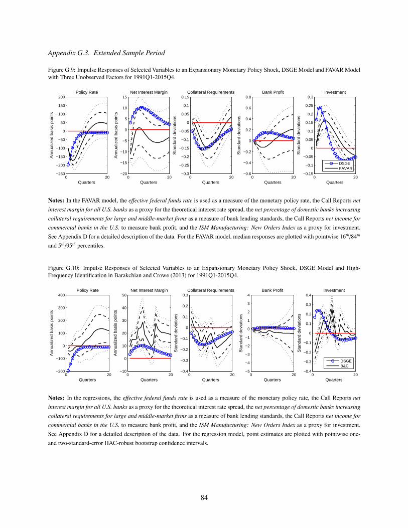
Appendix G.3. Extended Sample Period

Figure G.9: Impulse Responses of Selected Variables to an Expansionary Monetary Policy Shock, DSGE Model and FAVAR Modelwith Three Unobserved Factors for 1991Q1-2015Q4.

0 20−250

−200

−150

−100

−50

0

50

100

150

200Policy Rate

Ann

ualiz

ed b

asis

poi

nts

Quarters0 20

−20

−15

−10

−5

0

5

10

15Net Interest Margin

Ann

ualiz

ed b

asis

poi

nts

Quarters0 20

−0.3

−0.25

−0.2

−0.15

−0.1

−0.05

0

0.05

0.1

0.15Collateral Requirements

Sta

ndar

d de

viat

ions

Quarters0 20

−0.6

−0.4

−0.2

0

0.2

0.4

0.6

0.8Bank Profit

Sta

ndar

d de

viat

ions

Quarters0 20

−0.15

−0.1

−0.05

0

0.05

0.1

0.15

0.2

0.25

0.3Investment

Sta

ndar

d de

viat

ions

Quarters

DSGEFAVAR

Notes: In the FAVAR model, the effective federal funds rate is used as a measure of the monetary policy rate, the Call Reports net

interest margin for all U.S. banks as a proxy for the theoretical interest rate spread, the net percentage of domestic banks increasing

collateral requirements for large and middle-market firms as a measure of bank lending standards, the Call Reports net income for

commercial banks in the U.S. to measure bank profit, and the ISM Manufacturing: New Orders Index as a proxy for investment.

See Appendix D for a detailed description of the data. For the FAVAR model, median responses are plotted with pointwise 16th/84th

and 5th/95th percentiles.

Figure G.10: Impulse Responses of Selected Variables to an Expansionary Monetary Policy Shock, DSGE Model and High-Frequency Identification in Barakchian and Crowe (2013) for 1991Q1-2015Q4.

0 20−200

−100

0

100

200

300

400Policy Rate

Ann

ualiz

ed b

asis

poi

nts

Quarters0 20

−10

0

10

20

30

40

50Net Interest Margin

Ann

ualiz

ed b

asis

poi

nts

Quarters0 20

−0.4

−0.3

−0.2

−0.1

0

0.1

0.2

0.3Collateral Requirements

Sta

ndar

d de

viat

ions

Quarters0 20

−5

−4

−3

−2

−1

0

1

2

3

4Bank Profit

Sta

ndar

d de

viat

ions

Quarters0 20

−0.4

−0.3

−0.2

−0.1

0

0.1

0.2

0.3

0.4Investment

Sta

ndar

d de

viat

ions

Quarters

DSGEB&C

Notes: In the regressions, the effective federal funds rate is used as a measure of the monetary policy rate, the Call Reports net

interest margin for all U.S. banks as a proxy for the theoretical interest rate spread, the net percentage of domestic banks increasing

collateral requirements for large and middle-market firms as a measure of bank lending standards, the Call Reports net income for

commercial banks in the U.S. to measure bank profit, and the ISM Manufacturing: New Orders Index as a proxy for investment.

See Appendix D for a detailed description of the data. For the regression model, point estimates are plotted with pointwise one-

and two-standard-error HAC-robust bootstrap confidence intervals.

84

Figu

reG

.11:

Impu

lse

Res

pons

esof

Len

ding

Stan

dard

Mea

sure

sto

a25

bps

Exp

ansi

onar

yM

onet

ary

Polic

ySh

ock

inth

eB

asel

ine

FAVA

RM

odel

with

Thr

eeU

nobs

erve

dFa

ctor

sfo

r19

91Q

1-20

15Q

4.

020

−0.

50

0.5

Fed

eral

Fun

ds R

ate

020

−0.

50

0.5

Lend

ing

Sta

ndar

d 1

020

−0.

50

0.5

Lend

ing

Sta

ndar

d 2

020

−0.

50

0.5

Lend

ing

Sta

ndar

d 3

020

−0.

50

0.5

Lend

ing

Sta

ndar

d 4

020

−0.

50

0.5

Lend

ing

Sta

ndar

d 5

020

−0.

50

0.5

Lend

ing

Sta

ndar

d 6

020

−0.

50

0.5

Lend

ing

Sta

ndar

d 7

020

−0.

50

0.5

Lend

ing

Sta

ndar

d 8

020

−0.

50

0.5

Lend

ing

Sta

ndar

d 9

020

−0.

50

0.5

Lend

ing

Sta

ndar

d 10

020

−0.

50

0.5

Lend

ing

Sta

ndar

d 11

020

−0.

50

0.5

Lend

ing

Sta

ndar

d 12

020

−0.

50

0.5

Lend

ing

Sta

ndar

d 13

020

−0.

50

0.5

Lend

ing

Sta

ndar

d 14

020

−0.

50

0.5

Lend

ing

Sta

ndar

d 15

Qua

rter

s0

20−

0.50

0.5

Lend

ing

Sta

ndar

d 16

Qua

rter

s0

20−

0.50

0.5

Lend

ing

Sta

ndar

d 17

Qua

rter

s0

20−

0.50

0.5

Lend

ing

Sta

ndar

d 18

Qua

rter

s0

20−

0.50

0.5

Lend

ing

Sta

ndar

d 19

Qua

rter

s

Not

es:M

edia

nre

spon

ses

with

poin

twis

e16

th/8

4than

d5th

/95th

perc

entil

es.S

eeA

ppen

dix

Dfo

rade

taile

dde

scri

ptio

nof

lend

ing

stan

dard

mea

sure

s.

85

Figu

reG

.12:

Impu

lse

Res

pons

esof

Len

ding

Stan

dard

Mea

sure

sto

anE

xpan

sion

ary

Mon

etar

yPo

licy

Shoc

k,H

igh-

Freq

uenc

yId

entifi

catio

nin

Bar

akch

ian

and

Cro

we

(201

3)fo

r19

91Q

1-20

15Q

4.

020

−0.

50

0.5

Fed

eral

Fun

ds R

ate

020

−0.

50

0.5

Lend

ing

Sta

ndar

d 1

020

−0.

50

0.5

Lend

ing

Sta

ndar

d 2

020

−0.

50

0.5

Lend

ing

Sta

ndar

d 3

020

−0.

50

0.5

Lend

ing

Sta

ndar

d 4

020

−0.

50

0.5

Lend

ing

Sta

ndar

d 5

020

−0.

50

0.5

Lend

ing

Sta

ndar

d 6

020

−0.

50

0.5

Lend

ing

Sta

ndar

d 7

020

−0.

50

0.5

Lend

ing

Sta

ndar

d 8

020

−0.

50

0.5

Lend

ing

Sta

ndar

d 9

020

−0.

50

0.5

Lend

ing

Sta

ndar

d 10

020

−0.

50

0.5

Lend

ing

Sta

ndar

d 11

020

−0.

50

0.5

Lend

ing

Sta

ndar

d 12

020

−0.

50

0.5

Lend

ing

Sta

ndar

d 13

020

−0.

50

0.5

Lend

ing

Sta

ndar

d 14

020

−0.

50

0.5

Lend

ing

Sta

ndar

d 15

Qua

rter

s0

20−

0.50

0.5

Lend

ing

Sta

ndar

d 16

Qua

rter

s0

20−

0.50

0.5

Lend

ing

Sta

ndar

d 17

Qua

rter

s0

20−

0.50

0.5

Lend

ing

Sta

ndar

d 18

Qua

rter

s0

20−

0.50

0.5

Lend

ing

Sta

ndar

d 19

Qua

rter

s

Not

es:

Poin

test

imat

esw

ithpo

intw

ise

one-

and

two-

stan

dard

-err

orH

AC

-rob

ustb

oots

trap

confi

denc

ein

terv

als

base

don

dist

ribu

ted

lag

regr

essi

ons

ofea

chva

riab

leon

P=

4ow

n

lags

asw

ella

sco

ntem

pora

neou

san

dQ

=12

lagg

edob

serv

atio

nsof

the

exte

nded

shoc

kse

ries

.See

App

endi

xD

fora

deta

iled

desc

ript

ion

ofle

ndin

gst

anda

rdm

easu

res.

86

Figure G.13: Impulse Responses of Alternative Measures of Lending Standards to an Expansionary Monetary Policy Shock in theFAVAR Model with Three Unobserved Factors for 1991Q1-2015Q4.

0 20−0.1

−0.05

0

0.05

0.1

0.15(a) SLOOS Risk Tolerance

Quarters

Sta

ndar

d de

viat

ions

0 20−0.15

−0.1

−0.05

0

0.05

0.1(b) Excess Bond Premium

Quarters

Sta

ndar

d de

viat

ions

0 20−0.2

−0.15

−0.1

−0.05

0

0.05(c) NFCI Credit Subindex

Quarters

Sta

ndar

d de

viat

ions

Notes: Median responses with pointwise 16th/84th and 5th/95th percentiles, based on the FAVAR model with three unobserved

factors, where the 19 SLOOS lending standard measures have been replaced by (a) the net percentage of domestic banks easing

lending standards due to increased risk tolerance; (b) the excess bond premium proposed by Gilchrist and Zakrajsek (2012); (c) the

NFCI credit subindex published by the Federal Reserve Bank of Chicago. See Appendix D for a detailed description of the data.

Figure G.14: Impulse Responses of Alternative Measures of Lending Standards to an Expansionary Monetary Policy Shock, High-Frequency Identification in Barakchian and Crowe (2013) for 1991Q1-2015Q4.

0 20−0.8

−0.6

−0.4

−0.2

0

0.2

0.4

0.6

0.8(a) SLOOS Risk Tolerance

Quarters

Sta

ndar

d de

viat

ions

0 20−0.8

−0.6

−0.4

−0.2

0

0.2

0.4

0.6

0.8(b) Excess Bond Premium

Quarters

Sta

ndar

d de

viat

ions

0 20−0.8

−0.6

−0.4

−0.2

0

0.2

0.4

0.6

0.8(c) NFCI Credit Subindex

Quarters

Sta

ndar

d de

viat

ions

Notes: Point estimates with pointwise one- and two-standard-error HAC-robust bootstrap confidence intervals based on distributed

lag regressions of (a) the net percentage of domestic banks easing lending standards due to increased risk tolerance; (b) the excess

bond premium proposed by Gilchrist and Zakrajsek (2012); (c) the NFCI credit subindex published by the Federal Reserve Bank of

Chicago. See Appendix D for a detailed description of the data.

87

Appendices References

Angeloni, Ignazio, Ester Faia, and Marco Lo Duca (2013). “Monetary Policy and Risk Taking,” SAFE

Working Paper Series No. 8.

Amir Ahmadi, Pooyan and Harald Uhlig (2009). “Measuring the Effects of a Shock to Monetary Policy: A

Bayesian FAVAR Approach with Sign Restrictions.” Mimeo, Goethe University Frankfurt.

Barakchian, S. Mahdi and Christopher Crowe (2013). “Monetary policy matters: Evidence from new shocks

data,” Journal of Monetary Economics 60(8): 950-966.

Bassett, William F., Mary Beth Chosak, John C. Driscoll, and Egon Zakrajsek (2014). “Changes in bank

lending standards and the macroeconomy,” Journal of Monetary Economics 62(1): 23-40.

Bernanke, Ben S., Mark Gertler, and Simon Gilchrist (1999). “The Financial Accelerator in a Quantitative

Business Cycle Framework,” in: Taylor, J., Woodford, M. (Eds.), Handbook of Macroeconomics.

Bernanke, Ben S., Jean Boivin, and Piotr Eliasz (2005). “Measuring the Effects of Monetary Policy: A

FAVAR Approach,” Quarterly Journal of Economics 120(1): 387-422.

Carter, Chris and Robert Kohn (1994). “On Gibbs Sampling for State Space Models,” Biometrika 81(3):

541-553.

Christensen, Ian and Ali Dib (2008). “The Financial Accelerator in an Estimated New Keynesian Model,”

Review of Economic Dynamics 11(1): 155–178.

Christiano, Lawrence J., Roberto Motto, and Massimo Rostagno (2014). “Risk Shocks,” American Eco-

nomic Review 104(1): 27-65.

Geman, Stuart and Donald Geman (1984). “Stochastic Relaxation, Gibbs Distributions, and the Bayesian

Restoration of Images,” IEEE Transactions on Pattern Analysis and Machine Intelligence 6(6): 721-741.

Gilchrist, Simon and Egon Zakrajsek (2012). “Credit Spreads and Business Cycle Fluctuations,” American

Economic Review 102(4): 1692-1720.

Hodrick, Robert J. and Edward C. Prescott (1997). “Postwar U.S. Business Cycles: An Empirical Investiga-

tion,” Journal of Money, Credit and Banking 29(1): 1-16.

Kim, Chang-Jin and Charles R. Nelson (1999). “State-Space Models with Regime Switching: Classical and

Gibbs-Sampling Approaches with Applications,” MIT Press Books, The MIT Press, edition 1, volume 1,

December 1999.

Kadiyala, Rao and Sune Karlsson (1997). “Numerical Methods for Estimation and Inference in Bayesian

VAR-Models,” Journal of Applied Econometrics 12(2): 99-132.

Schmitt-Grohe, Stephanie and Martın Uribe (2006). “Comparing Two Variants of Calvo-Type Wage Sticki-

ness,” NBER Working Paper 12740, December 2006.

Taylor, John B. (2007). “Housing and Monetary Policy,” Proceedings – Economic Policy Symposium –

Jackson Hole: 463-476.

Townsend, Robert M. (1979). “Optimal Contracts and Competitive Markets with Costly State Verification,”

Journal of Economic Theory 21(2): 265-293.

88