Banking and Trading

Arnoud W.A. Boot and Lev Ratnovski

WP/12/238

© 2012 International Monetary Fund WP/12/238

IMF Working Paper

Research Department

Banking and Trading

Prepared by Arnoud W.A. Boot and Lev Ratnovski1

Authorized for distribution by Stijn Claessens

October 2012

Abstract

We study the effects of a bank's engagement in trading. Traditional banking is relationship-based: not scalable, long-term oriented, with high implicit capital, and low risk (thanks to the law of large numbers). Trading is transactions-based: scalable, short-term, capital constrained, and with the ability to generate risk from concentrated positions. When a bank engages in trading, it can use its ‘spare’ capital to profitablity expand the scale of trading. However, there are two inefficiencies. A bank may allocate too much capital to trading ex-post, compromising the incentives to build relationships ex-ante. And a bank may use trading for risk-shifting. Financial development augments the scalability of trading, which initially benefits conglomeration, but beyond some point inefficiencies dominate. The deepending of the financial markets in recent decades leads trading in banks to become increasingly risky, so that problems in managing and regulating trading in banks will persist for the foreseeable future. The analysis has implications for capital regulation, subsidiarization, and scope and scale restrictions in banking.

JEL Classification Numbers: G21; G24; G28; G32

Keywords: Bank regulation; proprietary trading; relationship banking; Volcker rule

Author’s E-Mail Address: a.w.a.boot@uva.nl and lratnovski@imf.org

1 We thank Stijn Claessens, Giovanni Dell’Ariccia, and George Pennacchi for helpful comments.

This Working Paper should not be reported as representing the views of the IMF. The views expressed in this Working Paper are those of the author(s) and do not necessarily represent those of the IMF or IMF policy. Working Papers describe research in progress by the author(s) and are published to elicit comments and to further debate.

2

Contents Page

I. Introduction ............................................................................................................................3

II. Relationship to the Literature ................................................................................................5 

III. Model ...................................................................................................................................6 A. Approach ...................................................................................................................6 B. Credit Constraints ......................................................................................................7 C. Banking .....................................................................................................................8 D. Trading ....................................................................................................................11 

IV. Benefits of Conglomeration ...............................................................................................12 

V. Time Inconsistency of Capital Allocation ..........................................................................14 A. Setup: Long-term Banking ......................................................................................14 B. The Consequences of Time Inconsistency ..............................................................16 C. Cost of Conglomeration under Time Inconsistency ................................................19 

VI. Trading as Risk-Shifting ....................................................................................................21 A. Setup: Risky Trading ..............................................................................................21 B. Risk-Shifting ...........................................................................................................23 C. The Interaction of Time Inconsistency and Risk Shifting .......................................27 

VII. Discussion ........................................................................................................................30 A. Front-loaded Income in Relationship Banking .......................................................31 B. External Equity and Internal Capital Allocation .....................................................33 C. Policy Implications ..................................................................................................34 

VIII. Conclusion ......................................................................................................................36  Figures 1. The Timeline .....................................................................................................................41 2. The Timeline with Time Inconsistency .............................................................................42 3. Relationship Banking Allocation R as a Function of Trading Opportunities ....................43 4. The Volume of Banking (R) and Trading (T), and Profits (Π) under Conglomerated Banking ......................................................................................44 5. The Volumes of Banking (R)and Trading (T), and Profits (Π) with Risk-shifting ............45 6. Time Inconsistency Arises due to a Higher Return to Trading under Risk-shifting (“Effect 1”) ...................................................................46 7. Risk-shifting Arises due to a Higher Volume of Trading, Driven by Time Inconsistency (“Effect 2”) ...............................................................................47 References ................................................................................................................................38

3

1 Introduction

We study the effects of a bank’s engagement in trading. We use the term “banking”

to describe business with repeated, long-term clients (also called relationship banking),

and “trading” for operations that do not rely on repeated interactions. This definition

of trading thus includes not just taking positions for a bank’s own account — propri-

etary trading — but also other short-term activities that do not rely on private and soft

information, e.g. originating and selling standardized loans. Both commercial and in-

vestment banks over the last decade have increasingly engaged in short-term trading.

We need to understand the rationale for that, and the challenges that it poses.1

Such challenges clearly exist. They are perhaps most vivid in Europe, where some

large universal banks seem to have over-allocated resources to trading prior to the crisis,

with consequent losses affecting their stability (e.g., UBS, see UBS, 2008; an earlier

example is the failure of the Barings Bank due to trading in Singapore in 1995). In the

United States, the development of universal banks was until recently restricted by the

Glass-Steagall Act. Yet there are many examples of a shift of institutions into short-

term activities, with similar negative consequences. Since early 1980-s, many New York

investment banks have turned the focus from traditional underwriting to short-term

market-making and proprietary investments; these have often backfired during the crisis

(Bear Stearns, Lehman Brothers, Merrill Lynch). Also, in 2000-s, commercial banks

have used their franchise to expand into short-term activities, such as wholesale loan

origination and funding (Washington Mutual, Wachovia), exposing themselves to risk.

And post-Glass-Steagall, there is evidence of trading being a drain on commercial bank

activities in newly created universal banks, such as Bank of America-Merrill Lynch. A

2012 loss related to the market activities in JP Morgan is another example. The banks’

short-term activities, especially proprietary trading, have received significant regulatory

attention: the Volcker Rule in the Dodd-Frank Act in the U.S., and the Report of the

Independent Commission on Banking (the so-called Vickers report) in the UK.

1More recently several banks have abandoned (or claim to have abandoned) trading activities in order

to focus on client-related business only. We are somewhat skeptical whether this is truly a long term

trend.

4

The interaction between banking and trading is a novel topic. The existing literature

on universal banks focuses primarily on the interaction between lending and underwrit-

ing. Such interaction is relatively well-understood, and also was not at the forefront

during the recent crisis. Our paper downplays the distinction between lending and

underwriting: for us both could possibly represent examples of long-term, relationship-

based banking.2 We contrast them to short-term, individual transactions-based activ-

ities. We see a shift of relative emphasis towards such “trading” as one of the major

developments in the financial sector (for sure prior to the crisis).

The focus on trading as a possibly detrimental activity in banks, and its difference

from underwriting in this regard, is supported by emerging empirical evidence. Brun-

nermeier et al. (2012) show that trading can lead to a persistent loss of bank income

following a negative shock. In contrast, underwriting, while more volatile than commer-

cial banking, is not associated with persistent losses of profitability.

The key to our analysis is the observation that the relationship business is usually

profitable and hence generates implicit capital, yet is not readily scalable. The trading

activity on the other hand can be capital constrained and benefit from the spare capital

available in the bank. Accordingly, relationship banks might expand into trading in order

to use ‘spare’ capital. This funding (liability-side) synergy is akin to the assertions of

practitioners that one can “take advantage of the balance sheet of the bank”.

Opening up banking to trading, however, creates frictions. We highlight two of

them. One friction is time inconsistency in the allocation of capital between the long-

term relationship banking business and the short-term trading activity. Banks may be

tempted to shift too much resources to trading in a way that undermines the relationship

franchise. Another friction is risk-shifting : the incentives to use trading to boost risk

and benefit shareholders as residual claimants. As a result of these two factors, a bank

can overexpose itself to trading, compared to what is socially optimal, or ex ante optimal

for its shareholders.

2Underwriting, insofar as it requires hard and codified information that is to be transmitted to the

markets, may have a lower relationship intensity that commercial bank lending based on soft information.

Nevertheless, at its core, underwriting remains a relationship-based activity.

5

Both problems become more acute when financial markets are deeper, allowing larger

trading positions. This increases the misallocation of capital and enables the gambles

of scale necessary for risk-shifting. The problems also become more acute when bank

returns are lower. Both factors have been in play in the last 10-20 years. Consequently,

the costs of trading in banks may have started to outweight its benefits. These fric-

tions are likely to persist for the foreseeable future, so a regulatory response might be

necessary.

The paper is organized as follows. Section 2 discusses the literature. Section 3 out-

lines the features of banking and trading, and sets up the model. Section 4 demonstrates

the benefits of conglomeration. Section 5 identifies the first cost of conglomeration —

the time-inconsistency problem. Section 6 deals with the other cost of conglomeration —

the risk-shifting problem, and the interaction between the two costs. Section 7 discusses

modeling features and policy implications. Section 8 concludes.

2 Relationship to the Literature

Our paper complements a number of strands in the banking and internal capital markets

literature. There is a vast literature on the costs and benefits of combining commercial

and investment banking, in particular whether underwriting that follows prior lending

relationships has biased standards (see Puri, 1996, and Krosner and Rajan, 1994, Fang

et al., 2010) or benefits from synergies (Schenone, 2004). While this literature focuses

on how borrower specific information is used across lending and underwriting activities,

our analysis focuses on combining banking (either lending or underwriting) with trading

activities that do not depend on borrower specific information.

In studying the problems of conglomeration, we focus on shareholder incentives. An

alternative approach would have been to consider the incentive problems of managers

(e.g. as in Acharya et al., 2011). While incentive issues in banks are undoubtedly

important, banks are subject to pressures from financial markets to maximize share-

holder returns. So understanding the distortions that can be caused by shareholder

6

value maximization alone remains important, particularly when such distortions may

have worsened in recent past because of external factors, such as increases in financial

market depth. Some papers have linked the distortions in bank trading activities to the

abuse of the safety net, including deposit insurance (Hoenig and Morris, 2011). Our

results are not driven by government guarantees, offering more general implications.

There is also a literature that studies how the expansion of markets affects bank

relationships (Boot and Thakor, 2000), and how financial market exuberance might

make banking highly procyclical (Shleifer and Vishny, 2010). We do not consider such

aspects. Instead we study how the core relationship business might be deprived of

resources and put at risk due to the presence of another activity — short-term trading —

in the same organization.

More generally, our paper relates to the literature on internal capital markets (Williamson,

1975, Danielson, 1984). Conglomeration may help relax the firm’s overall credit con-

straint (Stein, 1997) but also impose costs, primarily related to divisional rent-seeking

(Rajan et. al., 2000). Our model is similar in describing the benefits of conglomeration

as relaxing credit constraints, but points to a different set of costs: headquarters may

misallocate capital due to time inconsistency and risk shifting problems, which arise in

combining banking and trading. By analyzing a particular case of the misallocation of

resources, we can analyze the evolution of bank business models and draw implications

for the future.

3 Model

3.1 Approach

We describe a relationships-based business that we call “banking” and a transactions-

based business that we call “trading”. The banking activity relies on a fixed endowment

of information about existing customers; trading does not. We argue that this distinction

alone suffices to highlight a range of synergies and conflicts between the two businesses.

7

The fixed endowment of information makes the banking activity profitable (and, we

assume, not credit constrained), relatively safe, yet not scalable. Securing the value of

information requires non-contractible ex-ante investments that pay off over time; thus

banking becomes long-term in nature. In contrast, since it does not rely on any en-

dowment, trading is scalable, less profitable (and hence, we assume, credit constrained),

short-term oriented, and possibly risky.3

The fact that the banking activity has capacity for extra leverage (“spare capital”),

while trading is credit-constrained, drives the synergy between the two: conglomeration

can be used to expand the scale of trading. The potential conflicts between banking

and trading come from the differences in horizon and risk. Universal banks may choose

to over-allocate capital to trading because of the time inconsistency between long-term

returns of banking and short-term returns of trading, and because the risky trading

allows shareholders to engage in risk-shifting, unlike the safe banking activity. The

ex post over-allocation of capital to trading can compromise ex ante investments in

relationships, destroying the relationship oriented banking franchise.

The analysis proceeds in steps. We first set up a benchmark model of synergies

abstracting from the sources of conflicts. So, at the start, the time-consistency problem

and the possibility of risk shifting in trading are not present. We then introduce time-

inconsistency by making returns on banking dependent on ex ante decisions of customers

and distributed over time. This introduces the long-term nature of banking in contrast

to trading. After this we introduce risk-shifting by considering risky trading. We also

demonstrate the potential for mutual amplification between the time inconsistency and

risk-shifting problems.

3.2 Credit Constraints

A key feature of our model are credit constraints. We build on Holmstrom and Tirole’s

(1998, 2011) formulation that limits leverage based on the incentives of owner-managers

3One could characterize the banking activity as a high-margin-low-volume operation while trading

as a low-margin-high-volume operation.

8

to engage in moral hazard. We let the form of the credit constraint be identical for

standalone banking, trading, and the conglomerated activity. Assume that shareholders

can choose to run the bank normally, or engage in moral hazard (to obtain private

benefits). They will run the bank normally when:

Π ≥ (1)

where Π is the shareholder return when assets are employed for normal business, and

the right hand side is the shareholder return to moral hazard: a measure of bank

assets multiplied by the conversion factor 0 of assets into private benefits.4

There are many ways to interpret the payoff to moral hazard . They can repre-

sent savings on exerting the manager-shareholder’s effort (without which the relationship

banking projects do not repay, and trading strategies lose money), the possibility of ab-

sconding (Calomiris and Kahn, 2001), or limits on the pledgability of revenues (Farhi

and Tirole, 2011). When the incentive compatibility (IC) constraint (1) is not satis-

fied, shareholders engage in moral hazard and a bank becomes worthless for creditors;

anticipating this, creditors will not provide funding. This way, the IC constraint (1)

also describes the maximum leverage and, assuming decreasing returns to scale, the

maximum size of a bank.

We will now describe the banking and trading businesses.

3.3 Banking

Background We model relationship banking as based on a fixed endowment of in-

formation about customers, which allows the bank to obtain profits from serving them.

We do not distinguish between commercial banking (lending) and a client-oriented in-

vestment (underwriting) activity. Both share the key properties that we are interested

in:

4We do not consider the possibility of outside equity (assuming that it is very costly). See Section

7.2 for more discussion.

9

• Not scalable. It is prohibitively costly to expand the customer base at short notice.

• A valuable franchise (high charter value). A bank derives high returns from rela-

tionships, i.e. rents on its fixed endowment of information. It has therefore high

implicit capital. We thus assume that its leverage constraint is not binding: it has

spare borrowing capacity.5

• Low risk (certain return), due to the law of large numbers. A bank’s portfolio

contains multiple loans (or underwriting commitments) with independently dis-

tributed returns, making overall performance low risk (risk free in the model).

The certainty of returns combined with the high charter value implies limited

risk-shifting opportunities (in our model, non-existent). For example, sharehold-

ers of a bank with high franchise value and certain returns will fully internalize

the losses associated with choosing a low monitoring effort.6

• A long-term franchise. The return to relationship banking is distributed over timeand depends on customers’ ex-ante investment in relationships. We capture this

by assuming that part of the return on the banking activity is obtained in the

form of ex ante credit line fees paid by customers. If there are doubts about the

bank’s ability to make good on credit line commitments, the fees that customers

are willing to pay (their investment in relationships) decline. This intertemporal

feature (i.e. the long-term nature of banking) is introduced as a source of conflict

between banking and trading in Section 5. In the benchmark model of Section 4

we abstract from it.

Setup The bank operates in a risk-neutral economy with no discounting. It has no

explicit equity and has to borrow in order to invest; the risk-free rate on bank borrowing

is normalized to zero. There are three dates: 0, 1, 2.

5The rents imply some informational monopoly on the part of the bank; it may be related to past

investments by the bank and its customers into their relationships, and/or to advantages of proximity

or specialization in local markets. Note that the time and proximity elements involved in building

relationships provide a natural explanation for the lack of scalability.6 In the model, we abstract from aggregate risk. With a sufficiently high charter value, the presence

of aggregate risk would not affect the observation that risk-shifting opportunities are limited.

10

Franchise: informational rents. At date 0 the bank is endowed with private infor-

mation on a mass of customers. We let information produce a return for the bank in

two ways.

• First, it gives the bank implicit equity (franchise value) 0. An easy way to

introduce franchise value into our model is to assume that at date 0 the bank has

lent to customers with a repayment of (1 + )+0 at date 2 (hence obtaining

profits +0), while the measure of assets relevant for the IC constraint (1)

is the initial investment, . Substituting this into (1) gives a “wedge” between

profits and private benefits of 0. Since 0 plays a passive role in the model, we

streamline the exposition by setting = 0: it can be produced from a minimal

initial investment.

• Second, the bank has an opportunity to serve its customers’ future funding needs.Each customer is expected to have a liquidity need of size 1 at date 1 (with

certainty).7 When covering it, the bank can collect informational rents per

customer, up to a total of , from the repayment at date 2.

Spare borrowing capacity. We denote the amount that the bank borrows to cover the

customers’ liquidity needs at date 1 as ≤ . After borrowing, the bank can engage

in moral hazard to immediately obtain . The IC (leverage) constraint (1) takes the

form:

0 + ≥ (2)

where the left hand side is the bank’s market value of equity in normal operations: the

franchise value 0 and the information rent on covering its customers’ liquidity needs

. We assume that this constraint is satisfied, including at = , implying spare

borrowing capacity in banking:

0 + (3)

7For simplicity, we set the probability that the credit line will be used equal to one. We could envision

a probability less than one. For example, consider uncertainty about future market circumstances, with

the credit line only being used when external circumstances make it optimal because spot markets have

become ‘too expensive’ (cf. Boot et al., 1993).

11

3.4 Trading

Background The trading business is not based on an endowment of information.

Consequently, it has different properties:

• Scalable, with decreasing returns to scale. We think of decreasing returns to scale inthe context of a Kyle (1985) framework where the average return of an informed

trader falls in the size of her trade because the price impact increases in size.

The price impact is smaller when the mass of liquidity traders is larger. We can

therefore relate the diseconomies of scale to the depth of financial markets and, in

turn, to higher financial development, with lower diseconomies at higher depth.

• Less profitable, credit constrained. The return to trading is lower than the re-turn to banking because trading does not benefit from an endowment of private

information. As a result, trading, while scalable, can be credit constrained.

• Short-term. Unlike in banking, returns occur at one point in time and do not relyon ex ante investments.

• A possibility of risky (probabilistic) returns. A bank can choose between two trad-ing strategies. One generates safe but low returns. Another generates somewhat

higher returns most of the time, but can lead to catastrophic losses with a small

probability.8 We assume that the risky trading strategy has a lower NPV, yet a

levered bank may choose it to engage in risk-shifting. We introduce risky trading

in an extension of the model in Section 6.

Setup All trading activity is short-term. For units invested at date 1, trading

produces at date 2 net returns of for ≤ and 0 for . The parameter

captures the scalability of trading; it is natural to relate it to the depth of financial

markets, i.e. is increasing in the depth of the market. Trading is less profitable than

8This is reminiscent of banks taking on “tail risk” to generate “fake alpha” (see e.g. Acharya et al.,

2010).

12

banking since it does not benefit from the informational endowment:

(4)

And the low profitability of trading makes it credit constrained:

(5)

implying that the IC constraint (1) does not hold when trading is a standalone activity.

We thus, for simplicity, assume that standalone trading is not possible due to credit

constraints, despite the opportunity to profitably invest up to units.9

The timeline for the benchmark model is summarized in Figure 1. It abstracts from

the time inconsistency problem in banking (introduced in Section 5) and risk-shifting in

trading (introduced in Section 6).

4 Benefits of Conglomeration

Our model implies a natural benefit to the conglomeration of banking and trading: it

links a business with borrowing capacity but no investment opportunities (a relation-

ship bank) with a business that has investment opportunities but is subject to credit

constraints (trading).

Under conglomeration, at date 1, the bank maximizes profit:

Π = 0 + + (6)

subject to the joint leverage constraint (1):

0 + + ≥ (+ ) (7)

9The fact that, in our analysis, trading cannot exist as a stand-alone business should not be taken

literally. What is meant is that the viability of trading requires a substantial equity commitment. This

what we observe in most cases. Many independent trading houses are partnerships with substantial

recourse.

13

where ≤ . Comparing this to (3) and (5) shows that conglomeration allows for a

transfer of spare capital (borrowing capacity) from the relationship bank to the trading

activity.

The bank chooses the allocation of date 1 borrowing capacity between relationship

banking and trading to maximize profit. Since , the bank will choose to serve

all banking customers ( = ) before allocating any remaining capacity to trading.

The maximum amount of trading that a universal bank can support, max (assuming

max ≤ ) is given by (7) set to equality, with = :

max =0 + ( − )

− (8)

Since it is never optimal to trade at a scale that exceeds , = min { max}. Thismeans that when is low — the scalability of trading is small — the bank covers all

profitable opportunities in trading. When is high — trading is more scalable — the

bank covers trading opportunities max and abstains from the rest.

Proposition 1 (Conglomeration without frictions) The conglomeration of bank-

ing and trading enables expanding the scale of trading, which is otherwise credit-constrained.

In equilibrium, the bank serves all relationship banking customers, = , and al-

locates the rest of its borrowing capacity to trading, as long as trading is profitable,

= min { max}.

Proposition 1 is a benchmark that provides a rationale for why banks choose to

engage in trading, and specifies the first-best allocation of borrowing capacity between

the two activities. Next we study distortions that may arise in combining banking and

trading.

14

5 Time Inconsistency of Capital Allocation

5.1 Setup: Long-term Banking

The previous section has outlined the benefit of combining banking and trading — the

use of spare capital of the relationship bank to expand trading. We now turn to the costs

of conglomeration. This section deals with the first distortion: the time inconsistency

problem in capital allocation, induced by the different time horizon in banking (long-

term) and trading (short-term).

Banking is long-term because it involves repeated interactions with customers with

returns that are distributed over time and depend on ex ante investments in relation-

ships. Put differently, in relationship banking, a bank has the opportunity to serve its

customers’ future funding needs. We capture the intertemporal effects by assuming that

part of the returns come from ex ante credit line fees. By making these payments ex

ante (at date 0), customers reduce the payments they have to the bank ex post (at date

1). As a result, returns to banking, although higher than returns to trading, might

ex post be lower. This distorts capital allocation: once credit line fees have been col-

lected, a bank may have incentives to allocate too much capital to trading, leaving itself

with insufficient borrowing capacity to fully serve the credit lines. Anticipating that,

customers reduce the credit line fees that they are willing to pay ex ante, lowering the

bank’s overall profit and borrowing capacity. Section 7 discusses why the credit line

specification, capturing a front-loaded intertemporal allocation of returns and ex ante

investments in relationships, reflects an important feature of relationship banking.

Assume that, while a bank can generate return on covering customers’ future

funding needs, it can only capture ≤ through interest rates charged on the actual

lending between dates 1 and 2. The value of is limited by the potential for moral

hazard at the borrower level (Boyd and De Nicolo, 2005, Acharya et al., 2007). When

such moral hazard is severe, may be low. The remaining ( − ) can be captured at

date 0 as a credit line fee. Importantly, in our setup, a bank cannot commit to cover the

future liquidity needs of customers. That is, we let the bank have discretion to refuse

15

lending in the future if it has no borrowing capacity left to lend under the credit line.

The lack of enforceability implicit in this arrangement is similar to a real-life material

adverse change clause used in credit lines.10 The timeline incorporating the credit line

arrangement is shown in Figure 2.

At date 1, the bank chooses and to maximize its profit:

Π = 0 + ( − )− + + (9)

where − is the borrowing that customers expect to get under a credit line and

(−)− is the total credit line fee. is the actual borrowing under a credit line.

The bank maximizes (9) subject to the IC constraint:

0 + ( − )− + + ≥ (+ ) (10)

Note that in equilibrium, − = This follows since customers correctly anticipate

the bank’s ability and willingness to lend under the commitment.11

Recall that in the benchmark case in Section 4, the bank always covered the cus-

tomers’ liquidity needs, because the return on the banking activity was higher than that

on trading ( ), and time inconsistency problems were not present (ex post return and

total return were identical). Yet when a part of return to banking is obtained ex ante

to deal with potential moral hazard at the borrower level, time inconsistency problems

may interfere. As long as the ex post return to banking is sufficiently high, , there

is no diversion of borrowing capacity to trading. However when , the bank has

an incentive to divert borrowing capacity. In maximizing its ex post profit, the bank

chooses to first allocate the borrowing capacity to trading up to its maximum profitable

scale , and only then give the remainder to banking.

10The material adverse change clauses are ususally quite generally formulated and give a bank leeway

to refuse to lend under the credit line (claiming a general material adverse change on behalf of the

borrower).11As will become apparent, the bank will always charge the maximum possible amount, , ex-post.

That is, is set at the highest level such that the moral hazard problem at the borrower level is not

triggered. This minimizes the time inconsistency problem.

16

Whether the diversion of capital results in a misallocation away from banking de-

pends on the scalability of trading. When the scalability is low, ≤ max, the bank can

cover all liquidity needs of customers even after allocating to trading. That is, the

allocation {;|≤max} satisfies the leverage constraint (7). Hence, = and rela-

tionship banking does not suffer. However when scalability is high, max, banking

is credit constrained ex post : the allocation {;|max} no longer satisfies (7). Theborrowing capacity that remains after the bank has allocated to trading is insufficient

to cover all liquidity needs of customers, hence and relationship banking suf-

fers. Anticipating this, bank customers will pro-rate the credit line fee which they are

willing to pay ex ante based on the expected lending that the bank will offer ex post :

(−)− (−). The misallocation of borrowing capacity represents the timeinconsistency problem, and undermines the ability of a bank to maintain its relationship

banking franchise.

5.2 The Consequences of Time Inconsistency

Under time inconsistency ( and max), the bank chooses to allocate its

borrowing capacity to trading even when this means that it cannot deliver on the more

profitable banking activity. The severity of the consequences of the time inconsistency

problem depends on the relationship between the profitability of banking and the

private benefits . Observe that cutting back on banking conserves capital at a rate

(see IC constraint (1)) and undermines bank profitability at a rate . We will show that

only when the capital conservation exceeds the loss in profits some banking might

be preserved. There are two cases.

Case 1: . When is small, such that , cutting down on banking frees

up more capital than is lost in profits (the leverage constraint becomes slack), hence

trading can be expanded. This is the case when some banking may be preserved under

time inconsistency. That is, when the scalability of trading is not very high:

max ≤ 0

− (11)

17

we solve (10) as equality:

=0 − (− )

− (12)

=

These results give rise to interesting comparative statics. In this region of the interme-

diate scalability of trading, a diversion of borrowing capacity from banking to trading is

limited (the difference between and max). This misallocation is less severe at higher

levels of banking profitability : in (12) is increasing in , thus is closer to the

optimal allocation for higher . The reason is that a higher increases the franchise

value of the banking unit and allows it to offer more spare capital to trading. We can see

this from (8); at higher , more trading can be accommodated (max is higher), and this

reduces the the ex post diversion to trading (i.e. the difference between and max).

A higher scalability of trading:

0

− (13)

leads to all resources being allocated to the trading activity, and relationship banking

is wiped out. That is:

= 0 (14)

=0

−

Banking cannot be maintained now because the highly scalable trading can now accom-

modate all resources.

Case 2: ≥ . When is high, ≥ , it follows immediately from (8) that

max 0( − ). Given that — as is assumed — the time inconsistency problem is

present ( max), we now, contrary to Case 1, only have the higher range of scalability

in trading ( 0(−)). From Case 1 we know that trading will wipe out all bankingactivity in that range.

18

An alternative way to see this is to note that for cutting down on banking

leads to a loss in profits that is more than the capital freed up. This makes the leverage

constraint (10) more instead of less binding, reducing the capital available to trading. No

smooth reduction in the banking activity can help; in equilibrium, relationship banking

totally disappears. The time inconsistency problem is so severe that only trading remains

at a modest scale, based on the franchise value 0:

= 0 (15)

=0

−

The lessons that can be drawn from both cases are however subtle. Highly profitable

relationship banking ( ≥ ) allows for a substantial trading activity (i.e. max 0(−), see (8)) without a detrimental effect on the banking activity. If nevertheless the

scalability of trading exceeds this elevated level ( max), time inconsistency problems

in combining trading and banking will destroy the relationship banking franchise fully.

Hence we have a bang-bang solution.

At low levels of bank profitability ( ), the trading volume max that can be

accommodated is smaller. Time inconsistency sets in earlier, and from this point on

smoothly starts reducing the level of the banking activity. Not, however, that overall

the banking activity suffers more from trading in the case than in the case ≥ .

Figure 3 summarizes the dynamics of relationship banking under time inconsistency as

a function of trading opportunities.

Figure 3 can help interpret some fundamental changes in the financial sector. Over

the last decades, the deepening of financial markets has expanded trading opportunities.

With modest scalability of trading, banking did not suffer: time inconsistency was not

binding since the implicit capital of relationship banks could accommodate all trading.

Trading elevated overall bank profitability. Yet more recently two developments may

have undermined banks that engage in trading. (i) The scalability of trading may

have become too high, and (ii) developments in information technology (possibly the

19

same that have made trading more scalable) and deregulation may have reduced the

profitability of relationship banking. So trading has become more scalable, while

banking became less profitable and less able to support even the same levels of trading

without triggering detrimental time inconsistency. The former corresponds to the move

to the right on the axes of Figure 3, while the latter points to a shift from case 2 to case

1 in the figure (with lower max; note from (8) that max shrinks for lower values of ).

This migration provides some important lessons for the industry structure of banking.

With limited trading opportunities and relatively profitable banking activities, there is

substantial scope for combining banking and trading. However, more scalable trading

coupled with less profitable banking can undermine banking severely. Combining the

activities then becomes very costly.

The dynamics of and for cases and ≥ , without (as in Section 4) and

with time inconsistency (this section), are summarized in Figure 4, panels A and B.

Proposition 2 (Time inconsistency) When a part of the return to banking is col-

lected ex-ante, the profitability of banking is low (low 0 and leading to low and max)

and/or trading is sufficiently scalable (high ), a bank may have incentives to allocate

ex-post more borrowing capacity to trading than what is ex-ante optimal. Specifically,

when , then for max, the bank will allocate insufficient capital to serving the

future funding needs of its customers: . Anticipating this, ex-ante investments in

banking suffer: customers pay lower credit line fees, compromising relationship banking.

5.3 Costs of Conglomeration under Time Inconsistency

We can now derive bank profits. Recall that the cumulative profit of banking and trading

as standalone activities is:

Π = 0 + + 0 = 0 + (16)

20

where 0 + is the profit of a standalone relationship bank (see (3)), and zero is the

profit of standalone trading (which is not viable).

The profit of a bank that engages in trading depends on the scalability of trading,

. For ≤ max, time inconsistency is not present, and the profit is increasing in :

Π = 0 + + (17)

For higher , max, Π is decreasing in as time inconsistency distorts capital

allocation. Following the two cases in Section 5.2: for a bank substitutes trading

for banking, and its profit decreases smoothly (use (12)) until the maximum feasible

scale of trading = 0( − ) is reached:

Π = 0 +0 − ( − )

− , for max ≤ 0(− ) (18)

Π = 0 + 0

(− ), for 0(− ) (19)

For ≥ , cutting down on banking does not create borrowing capacity for trading.

Hence, the banking activity collapses for max, leading to a discrete drop in profit

at = max, to the level given in (19). The profits of a conglomerated bank depending

on the scalability of trading are summarized in Figure 4, panels C and D.

Overall, from (17-19), we observe that, in comparison to stand-alone banking, the

engagement in trading increases profitability initially (for low ) but can lead to a loss

of profitability for higher . Specifically, when a bank fully substitutes trading for

relationship banking ( = 0; = 0(− )) its profit Π as given in (19) is less than

the standalone profit Π (see (16)) when relationship banking rents are sufficiently

high:

0

(− )(20)

The results can be summarized as follows:

Proposition 3 (Profits with time inconsistency) The effect of conglomeration on

21

bank profits is inverse U-shaped in trading opportunities . For low opportunities (

max), time inconsistency is not present, and profits increase in trading opportunities

as a bank can better use its spare capital. For large opportunities ( max), profits

fall with additional trading as the time inconsistency problem intensifies. There exist

parameter values such that beyond a certain scale of trading opportunities, banks that

do not engage in trading generate higher profits than banks that combine relationship

banking and trading.

6 Trading as Risk-Shifting

6.1 Setup: Risky Trading

The previous section has identified an important distortion that may arise when banks

engage in trading: a time inconsistency in capital allocation, which can damage the

bank’s relationship franchise. This section discusses a related distortion: the use trading

for risk-shifting. We also study how the two problems interact.

Shareholders of a leveraged firm have incentives for risk-shifting when risk (funding)

is not fully priced at the margin (Jensen and Meckling, 1978). The latter is a standard

feature of corporate finance, and arises when funds are attracted before an investment

decision, to which shareholders cannot commit. Risk not priced at the margin is certainly

present in banks.12

Yet, generating risk-shifting in traditional relationship banking might be difficult.

Risk-shifting requires probabilistic returns: an upside that accrues to shareholders and

12The pricing of risk might be more distorted in banks than in non-financial companies. One reason is

the safety net (for insured deposits or “too big to fail” banks). Government bailouts of failing banks can

subsidize risk taking. Another reason are the effects of seniority, when newly attracted funding is senior

to existing debt due to the use of collateral (Gorton and Metrick, 2010), short maturities (Brunnermeier

and Oehmke, 2011), or higher sophistication (Huang and Ratnovski, 2011). Then, new funding is

effectively subsidized by existing creditors (although the latter may anticipate such risk transfer and

charge higher interest rates ex ante). In addition to these, a possibly higher liquidity of bank assets

compared to industrial firms may make it easier for banks to opportunistically change their risk profile

(see Myers and Rajan, 1998). We do not need these additional effects in our model. But if present,

they would strengthen our results. In particular, while we proceed to assume a positive NPV of risky

trading, having risk subsidized may give the bank incentives to engage in risky trading even if it has a

negative NPV.

22

a downside that exceeds the franchise value and imposes losses on creditors. But re-

lationship banking is a rather stable activity with relatively predictable returns. For

example, in commercial or investment banks that have multiple loans or underwriting

operations with uncorrelated outcomes, the return is close to certain due to the law

of large numbers (save for the exposure to the business cycle). With high franchise

value, shareholders will internalize all consequences of their moral hazard, for example

absorb losses associated with a somewhat higher share of non-performing loans that may

arise because of insufficient monitoring. In contrast, trading allows the bank to generate

highly skewed returns, for example, from large undiversified positions. Then, for a bank,

trading becomes not just a profit opportunity, but a means to perform risk-shifting.

To model risk-shifting, we introduce risky trading. Assume that a bank can choose

between a safe trading strategy considered before and a risky trading strategy, which

for units invested generates a gross return (1 + + ) with probability , and 0

with probability 1 − , up to the maximum scale of trading . The binary return is a

simplification, representing a highly skewed trading strategy. The notion is that banks

use trading to generate extra return “alpha” by taking bets that are safe in most states

of the world, but occasionally lead to significant losses. Such behavior is supported by

the accounts of the strategies employed in the run-up to the financial crisis (Acharya et

al., 2010).

We assume that risky trading has a lower NPV than safe trading, yet positive:

0 (1 + + )− 1 (21)

so that a bank would only choose risky trading for risk-shifting purposes, and, as long

as there is spare borrowing capacity, will choose some some trading instead of leaving it

unused.

At the same time, holding the cost of debt fixed, the risky trading has a higher return

than safe trading, creating incentives for shareholders to use trading for risk-shifting.

Yet, the return to risky trading is not as high as to make IC constraint (1) less binding

23

in the larger volume of trading:

(+ ) (22)

The choice of the trading strategy is not verifiable.

Under risky trading, a bank may be unable to repay its creditors in full. Shareholders

then surrender available cash flows to creditors. Since the bank may choose to engage

in risk-shifting, the interest rate charged by its creditors is no longer necessarily zero.

Instead, creditors ex ante set the interest rate based on their expectations of the bank’s

future trading strategy (achieving zero expected return). For simplicity, we assume

that when multiple equilibria are possible, the creditors set the lower rate. The bank

chooses safe trading when indifferent. We focus on the richest case that combines time

inconsistency ( ) and a smooth contraction of banking ( ).

6.2 Risk-Shifting

We first derive conditions under which the bank would choose risky trading when charged

a low interest rate = 0. This allows us to define a threshold level of beyond which a

bank would shift to risky trading. We then characterize the risky trading equilibrium —

interest rates, capital allocation, and profits.

Assume that = 0 and consider the payoff to risky trading. When a bank invests

in relationship banking and in risky trading, it obtains at date 2 from relationship

banking 0+(1+); and from trading (1 + + ) with probability and 0 otherwise.

The bank has to repay creditors + . It can do so in full when trading produces a

positive return. Yet when trading produces a zero return, the bank has sufficient income

to repay in full only if 0+ (1+ ) ≥ + , corresponding to an upper bound on the

volume of trading:

≤ 0 + (23)

When (23) holds, the bank’s debt is safe, and shareholders internalize the losses from

24

risky trading. Their payoff is:

Π|≤0+ = 0 + + (1 + + ) − (24)

This is lower than the payoff with safe trading: Π|≤0+ Π where Π is

given in (6). By (21), risky trading has a lower NPV than safe trading. Hence, bank

shareholders will never choose risky trading if they fully internalize possible losses.

We thus focus on the case 0+ , where a bank cannot repay creditors in full

when a risky trading strategy produces zero. Here, the shareholders’ return when the

bank engages in risky trading is:

Π = (0 + + (+ ) ) (25)

We can now compute the threshold level of trading beyond which the bank chooses risky

trading. This happens when Π Π , giving (use (6) and (25)):

=(0 + ) (1− )

(+ )− (26)

From the inequality (26) it follows that the bank will choose risky trading when trading

has a high scale ( ), or when the value of the relationship banking franchise

(0+ ) is low. The reason is that risky trading effectively has a fixed cost, the loss of

the relationship banking franchise value (0 + ) with probability , while its benefit,

the additional return , is proportional to the scale of trading. Hence the scale of trading

has to be high enough to compensate for putting the relationship banking franchise at

risk.

We can now complete the analysis by deriving the bank’s choice of the trading

strategy and the allocation of borrowing capacity as functions of the scalability of trading

. We start by endogenizing as given in (26). When a bank allocates to trading,

25

the borrowing capacity left to banking (from (10) is:

=0 − (− )

− (27)

Substituting this into (26) gives:

=0(1− )

((1− )− ) + (− (1− ))(28)

We can verify the following:

Lemma 1 (i) 0 and 0: when risky trading has a higher

upside and a lower risk, the switch to risky trading occurs at a lower scale;

(ii) 0 0 and 0: when the relationship franchise value is

higher, the switch to risky trading occurs at a higher scale.

Proof. All are obtained by differentiation and considering that:

(i) The denominator in (28) is positive:

(− (+ )) + (− (1− )) = [(− )+ (1− )( − )] 0

since and

(ii) The expression ((1− )− ) in the denominator of (28) is negative. Use (22)

to see that:

(1− )− (+ )(1− )−

and

(+ )(1− )− = (− (+ )) 0

We can now derive the allocation of borrowing capacity, interest rates and profits

under risky trading. To limit attention to the more insightful case, we focus on the case

26

when max. Risk-shifting is then only relevant when the time inconsistency

problem is present.

Then, for ≤ the bank chooses the safe trading strategy with the allocation

of the borrowing capacity given by (12). For , the bank chooses risky trading.

Note that when there is time inconsistency in the allocation of borrowing capacity in

safe trading ( ), it also exists in risky trading because ( + ) (see (22)),

where ( + ) is the ex post return to risky trading. Therefore, under risky trading,

the bank will also first allocate the maximum possible borrowing capacity to trading

before using the remainder for banking. The interest rate follows from the creditors’

zero-profit condition:

(+ ) = (+ ) (1 + ) + (1− )(0 + (1 + )) (29)

where ( + ) is the amount borrowed by the bank, (+ ) (1 + ) is the debt re-

payment when risky trading succeeds, and (1− )(0 + (1 + )) is the value of bank

assets transferred to creditors in case of bankruptcy. The borrowing capacity left for

the banking activity follows from the IC condition (set to satisfy with equality):

(0 + ( − )+ (+ − ) ) ≥ ( +) (30)

where the left hand side is the expected payoff to bank shareholders in normal operations,

and the right hand side is the moral hazard payoff.

As in (12) through (14), for ≤ 0

−((1++)−1), we obtain:

=0 − ((1− ) + − (+ ))

− (31)

=

27

And for 0

−((1++)−1):

= 0 (32)

=0

− ( (1 + + )− 1)

Similarly to (18) and (19), bank profits are:

Π =

µ0 +

0 − ( − ((1 + + )− 1))−

¶, for ≤ 0

− ( (1 + + )− 1)(33)

Π =

µ0 +

((1 + + )− 1)0

− ( (1 + + )− 1)¶, for

0

− ( (1 + + )− 1) (34)

Note that the shift to risky trading has two negative effects. First, it has a direct

negative effect on bank profits because the risky trading has a lower NPV than safe

trading. Although shareholders do not internalize this ex post, they internalize it ex

ante through higher interest rates on bank borrowing. Second, lower bank profits reduce

bank borrowing capacity, and thus further undermine bank profitability. As a result,

Π Π (compare (33) and (34) to (18) and (19)). The dynamics of and

and the evolution of bank profit when the bank can use trading for risk-shifting are

demonstrated in Figure 5.

Proposition 4 (Risk-shifting) The bank may engage in risky trading as a form of

risk-shifting, when the profitability of banking ( and 0) is low and/or trading is suffi-

ciently scalable ( ). This is detrimental to bank profits, as the bank internalizes

the costs of risk-shifting through higher borrowing costs.

6.3 The Interaction of Time Inconsistency and Risk Shifting

Finally, we study the interaction between time inconsistency and risk shifting problems

in banks that engage in trading. There are three effects, by which the two problems can

amplify each other, so that the presence of one distortion makes the presence of another

more likely.

28

Effect 1. Risk-shifting makes time inconsistency more likely by increasing the ex

post return on risky trading. Recall that ( + ). Thus the ex-post return from

trading is higher with risky trading. This creates the region:

(+ )

where the time inconsistency problem arises only under risk-shifting. That is, there was

no time inconsistency in the absence of risky trading ( ), but it is present under

risky trading ( ( + )). To see this not that for such parameter value, a bank

chooses safe trading and there is no time inconsistency for max : when

risk shifting is not present. Yet for a bank chooses risky trading, and that

risky trading also triggers time inconsistency. See Figure 6.

Effect 2. Time inconsistency makes risk-shifting more likely by increasing the equi-

librium volume of trading. Consider two cases. In case 1, (+), so the time incon-

sistency problem is not present. The maximum volume of bank trading is max (8). Since

≥ max, the bank will never engage in risk shifting since the equilibrium scale of

trading is too low to make risk-shifting worthwhile. In case 2, , and the time in-

consistency problem is binding for max. Then, time inconsistency can increase the

equilibrium scale of trading beyond max. When max 0(−((+)−1)),the bank will start engaging in risk shifting as a result of the higher scale of trading,

driven by the time inconsistency problem. See Figure 7.

Effect 3. Time inconsistency makes risk-shifting more likely by reducing the rela-

tionship bank’s franchise value. The risk to the bank’s franchise value (its loss with a

probability (1 − )) is the cost of risk shifting. To show the interaction between time

inconsistency, franchise value and risk-shifting, we need to enrich the model. Assume

that the presence of the time inconsistency problem is uncertain at date 0. Specifically,

at date 0 there is a probability that at date 1 = , and there is no time

inconsistency; and with probability 1 − = , and hence time inconsistency

is present. This allows us to show the ex post consequences of different expectations

29

of time inconsistency on the bank’s franchise value, and through it on the threshold

value (28).

Consider the realization = at date 1, so that time inconsistency is present.

Then, at date 1, the payoff to bank shareholders from the safe trading is:

Π = 0 + ( − )

¡+ (1− )−

¢+ + (35)

The expression Π is similar to Π in (9), except for the second term — higher credit

line fees that the customers are willing to pay the bank at date 0. Time inconsistency

now arises not with probability 1, but with probability 1 − ; hence compared to (9)

credit line fees (and bank franchise value) are higher by ( − ) ¡−−

¢.

Similarly, the payoff from risky trading is:

Π =

¡0 + ( − )

¡+ (1− )−

¢+ + (+ )

¢(36)

Setting = − and equating Π and Π

as given in (35) and (36) provides the

threshold point for a switch to risk-shifting (similar to (26)):

=

¡0 + ( − )

¡−

¢+

¢(1− ))

(+ )− (37)

Observe that a higher elevates the bank’s franchise value at date 2. First, it

increases the credit line fees by ( − ) ¡−−

¢. Second, it increases the bank’s

borrowing capacity, increasing the value of for any given . Therefore,

0:

risky shifting becomes less likely under less intensive time inconsistency, as the bank

must have a higher scale of trading to compensate for a higher cost of compromising

bank franchise value.

Proposition 5 (Interaction of time inconsistency and risk-shifting) The prob-

lems of time inconsistency and risk shifting amplify each other. Time inconsistency

increases the scale of trading and reduces franchise value of the relationship bank, in-

30

creasing incentives for risk-shifting. Risk-shifting increases the bank shareholders’ ex-

post return from trading, which may trigger time inconsistency in capital allocation.

7 Discussion

At this stage it is useful to summarize the distortions in banks that engage in trading,

and how they may have changed over time. There are two distortions: one is the time

inconsistency of capital allocation where a bank may choose to trade on a scale that

is too high at the expense of its relationship banking franchise. The second is the use

of trading for risk-shifting. Both distortions are more likely when the profitability of

banking is low and the scalability of trading is high. These factors may have come

into play in recent decades due to developments in information technology, facilitating

easier access to information benefiting trading (increasing ) and reducing the grip that

banks have over their relationship borrowers. The latter would reduce the profitability

of banking (reduce 0 and ).

Moreover, our analysis points to several reinforcing effects. First, as we show in

Propositions 2 and 4, the effects of higher scalability of trading and lower profitability of

banking work in the same direction and reinforce each other. Second, time inconsistency

and risk-shifting also arise simultaneously, and amplify each other as well (Proposition

5). Overall, this implies that trading and other transactional activities in banking, while

possibly benign and beneficial historically, might recently have become destructive: i.e.

undermining the viability of relationship banking and putting banks at risk. These

implications appear consistent with the evidence from the recent crisis.

We now discuss some modeling features, in particular, the approach the modeling

relationship banking, limits to external equity and commitment problems in capital

allocation, and sum up key policy implications.

31

7.1 Front-loaded Income in Relationship Banking

This paper characterized relationship banking as a business requiring ex ante invest-

ments in relationships, which produce returns distributed over time. The intertemporal

nature of commitments is indeed a key feature of relationship banking.

We have modeled the time dimension of relationship banking returns through a

credit line contract with ex ante fees. Our formulation thus focuses on the “front-loaded

income” from relationships, where a bank obtains profit early on, but needs to be able

to honor future commitments. There is ample evidence that relationship banks indeed

play a large role in providing liquidity insurance (or, more generally, funding insurance)

to customers. Often, such role is played by local banks, which possess information on

borrowers and local market conditions that is crucial to evaluate the borrower’s state of

affairs, especially in negative economic circumstances.

As we highlight in this paper, the “funding insurance” role brings potential time-

inconsistency problems. Banks typically have discretion in deciding whether to honor

lending commitments as most include “material adverse change” (MAC) clauses that

give them an option to renege. In particular, we argue that shifting capital to the trading

business ex post may undermine the bank’s ability to expand relationship lending when

requested, and render “insurance” relationships less valuable for borrowers and less

profitable to the bank.

Observe that the credit line (with discretionary MAC clause) that we model is a par-

ticular way of structuring the relationship. The client is willing to get services/products

from its relationship bank, possibly even pay a slight premium over market (transaction)

prices, in return for knowing that the bank relationship might be valuable in stressful

times. While we have in mind (and in the model) times of stress that the borrower faces,

we do observe that a bank that faces stressful times typically prioritizes its limited (risk

bearing) capacity to its relationship clients, and also in this way insures it relationship

banking clientele.

Whether banks actually deliver when such need arises affects the reputation of the

32

bank, and more generally the competitive position of the bank; e.g. the ease with which

it can hold on to its customers. More reputable banks might be less opportunistic,

and less susceptible to diversions of borrowing capacity to trading. In this context

also a bank’s credit rating is relevant. The rating may in part reflect the risk bearing

(or, lending) capacity that is not filled up opportunistically. Hence, borrowers may

anticipate that banks with higher rating are better able to deliver on (implicit) promises

or guarantees about future funding availability. This could explain why ratings are of

such importance in the financial services industry.

The way we have modeled relationship banking, i.e. via the credit line contracting

feature, can be seen as capturing a variety of circumstances where banking is based on

ex-ante investments and future funding commitments. One such example is syndicated

lending, where banks that are part of the syndicate have a mutual understanding to try

to accommodate requests to participate in each others’ syndicated projects. Reputation,

including having a good credit rating, may again be a key factor in convincing others that

a bank might be able to deliver and play its part in the reciprocity based syndicated

lending market. Another example are commitments to local markets based on the

knowledge of customers which facilitates funding in times of economic stress.

Another feature of relationship banking commonly postulated in the literature is

“back-loaded income”, where borrowers are subsidized initially, while hold-up problems

allow the bank to recoup the subsidies later (Petersen and Rajan, 1995; Boot and

Thakor, 2000). This makes the relationship banking business more attractive ex post

since the bank has already made investments ex ante. A bank with high future rents

from relationships is less likely to be exposed to time inconsistency problems or to engage

in risk-shifting. Yet, the ex post rents in banking have been reduced in the recent past

due to higher competition and more easily available borrower information reducing the

informational advantage of banks (Keeley, 1990). Hence, the “front-loaded” aspect of

relationship banking that we analyze in the paper may have become more important.

33

7.2 External Equity and Internal Capital Allocation

Two important features of our analysis are frictions in the internal allocation of capital

(the time inconsistency problem) and difficulties in accessing external equity. The latter

could help explain why trading activities might have to be undertaken in conjunction

with a relationship bank: if attracting external capital is costly, using the implicit capital

of the relationship bank (its franchise value) could offer convenient access to capital.

In our analysis, it is always optimal for banks to use their excess capital for trading.

Suboptimality only comes in when too much is allocated to trading due to the time

inconsistency problem. Costly outside equity also explains why the time inconsistency

problem is really bad for the relationship banking franchise: the capital that is diverted

to trading cannot be easily replaced.

A natural question is whether the bank could have preempted the diversion of capital

to trading by returning it back to shareholders (e.g. via dividends or share buybacks).

The answer is no. To understand this, note that besides excess capital (which the

relationship bank cannot use due to a fixed customer base, and which indeed could

be returned to shareholders), the relationship bank in the normal course of business

maintains unused capital (spare borrowing capacity) in order to cover future funding

needs of customers. The model highlights that such capital can be misallocated to

trading, making the bank unable to fulfill its relationship commitments. But if this

unused capital was returned to shareholders, the bank would still be unable to make

good on its commitments. Hence, the relationship franchise would be destroyed in either

case; returning capital to shareholders cannot resolve the problem of time inconsistency.

The problem of time inconsistency between short- and long-term activities that we

focus on in this paper is reminiscent of the literature that shows how trading at an

intermediate moment in dynamic models of financial intermediation might undermine

commitment (see for example the Jacklin (1987) comment on the Diamond and Dybvig,

1983). Other, more general examples of the negative effects of short-term bank activities

on commitment include a lack of shareholder discipline under unstable and diffused

34

ownership (Bhide, 1993), increased ease of asset transformation moral hazard (Myers

and Rajan, 1998), or the increased sensitivity of decisions to short term financial market

pressures (Shleifer and Vishny, 2010).

7.3 Policy Implications

The paper offers two contributions to the policy debate. The first contribution is a set

of stylized facts (predictions) that are useful for understanding the dynamics of banks

that engage in trading. We suggest that:

• Relationship banks are tempted to ‘use their balance sheet’ (i.e. implicit capi-tal) for scalable trading opportunities. While limited trading can enhance bank

profitability and franchise value, excess trading can reduce profits and destroy the

relationship banking franchise.

• Financial development has undermined trading in banks through two channels:more scalable trading and less profitable relationship banking (possibly due to

higher competition and better available customer information). Both increase

incentives to over-allocate capital to trading, and to use trading for risk-shifting.

• In the above, the activities that suffer most would be those that involve discre-tionary contracting: credit lines (with MAC clauses), syndicated lending (with

reciprocity to syndicated banks), and in general commitments to customers to

offer funding in periods of economic stress based on local knowledge (see Section

7.1). In the presence of time inconsistency such contracts become less valuable

and may no longer be viable. Banking as a whole becomes more transactional.

• A broad implication from the increased intensity of the time inconsistency and riskshifting problems is that combining banking and trading (the traditional European

universal bank model, shared by some U.S. conglomerates) might have become

less sustainable. Universal banks have historically combined a sizable relationship

banking activity with a much smaller transactions-based activity. Now banks

35

might allocate too many resources to the transactional activity, leading to lower

profit and higher risk.

The second contribution is to the debate on restricting the scope of banking. Broadly

speaking, the policy debate has focused on two (possibly complementary) approaches:

prohibiting trading in banks (specifically proprietary trading: the Volcker rule) or segre-

gating trading and other market-based activities (including underwriting) into firewalled

subsidiaries (the approach of the U.K. Independent Commission on Banking, “the Vick-

ers Commission”). Our analysis, based on identifying two underlying market failures

— the time inconsistency and risk-shifting problems — allows us to make the following

observations:

Scope of restrictions. The market failures identified in our model are driven by banks

engaging in trading: transactional (short-term, scalable) activities. Observe that Vickers

separates from banks more than trading: not all market-based activities are transac-

tional in nature; some — notably underwriting — are commonly relationship-based. The

rationale for segregating them from banking is unclear. At the same time, Volcker might

be too narrow in focusing solely on proprietary trading and not on other transactional

bank activities (e.g. investing in structured assets).

Segregating vs. prohibiting. Segregating trading into a separate subsidiary (Vickers)

might help alleviate the risk-shifting problem. It can reduce risk spillovers from trading

to the relationship bank, and offer transparency and a more risk-sensitive pricing of

the funding for trading. The limitation is that segregation may not be able to prevent

reputation-based recourse, i.e. when the relationship bank voluntarily chooses to cover

losses in trading (as was the case in the number of episodes in the recent crisis). However,

segregating trading cannot resolve the time inconsistency problem. Similar to Section

7.2 above, even if some trading activities were segregated into a separate subsidiary, a

bank would still have incentives to misallocate to trading the capital that it maintains

for future funding needs of customers (maintaining lending capacity). Put differently,

even with segregated trading a bank might trade too much; it might allocate too much

36

capital to trading subsidiaries and too little to banking subsidiaries. A prohibition of

proprietary trading (Volcker) — and more broadly of other transaction-based activities

— in banks and banking groups might thus be essential to prevent time inconsistency.

Trading-like activities that are part of the lending process. A key implementation

challenge to Volcker or Vickers is that a restriction on trading might affect market ac-

tivities that are inherent to relationship lending, such as taking positions for hedging

purposes. With caution, one could build on a “middle ground” suggested by our analysis.

Banks could be allowed to undertake market operations but on a limited scale. Trading

in low volumes (below max (20) and (28)) does not trigger time inconsistency

(capital misallocation is too small) or risk-shifting (bank shareholders sufficiently inter-

nalize the costs of risky trading). Trading on a limited scale would not create distortions

but will give banks space to undertake market operations that are necessary to support

the lending process.

Capital regulation. Our analysis highlights the importance of maintaining spare

capital in a relationship bank for serving future funding needs of customers. Thus

relationship banks, while inherently safe, need to operate at levels of capital sufficiently

in excess of the regulatory minimums to have the flexibility necessary to fulfil their

relationship commitments. This is consistent with the proposed role of procyclical and

other capital surcharges (assuming that banks can draw upon those sources of capital

relatively freely), as opposed to fixed high capital requirements, in supporting the supply

of banking services over the business cycle.

8 Conclusion

The paper studies incentive problems in universal banks that combine relationship bank-

ing and trading operations. Banks have incentives to engage in trading since that allows

them to use the borrowing capacity of the relationship bank to profitably expand the

scale of trading. However it generates two inefficiencies. Universal banks may allocate

too much capital to trading ex-post, compromising the incentives to build relationships

37

ex-ante. And universal banks may use trading for risk-shifting, compromising bank

stability.

Financial development augments the scalability of trading, which initially benefits

conglomeration, but beyond some point inefficiencies dominate. The proliferation of

financial markets and increased financial deepening in recent decades suggest that con-

glomeration faces severe head winds such that problems in managing and regulating

universal banks will persist for the foreseeable future. Our results highlight the dynamic

problems in universal banking and sheds light on the desirability of restricting bank

activities of the type that were recently proposed by the Volcker rule in the U.S. and

the Vickers report in the UK.

38

References

[1] Acharya, V.V., T.F. Cooley, M.P. Richardson, and I. Walter, 2010, “Manufacturing

Tail Risk: A Perspective on the Financial Crisis of 2007-09”, Foundations and

Trends in Finance, 4.

[2] Acharya, V.V., M. Gabarro and P. Volpin , 2011, “Competition for Managers, Cor-

porate Governance and Incentive Compensation”, mimeo London Business School.

[3] Bhide, A. (1993), “The Hidden Cost of Stock Market Liquidity”, Journal of Finan-

cial Economics, Vol. 34(1), p. 31-51.

[4] Boyd, J. and G. De Nicolo, 2005, “The Theory of Bank Risk-Taking and Competi-

tion Revisited” Journal of Finance, Vol. 60(3), p. 1329-1343.

[5] Boot, A.W.A., S.I. Greenbaum and A.V. Thakor, 1993, “Reputation and Discretion

in Financial Contracting”, American Economic Review, Vol. 83(5), p. 1165-1183.

[6] Boot A.W.A. and A.V. Thakor, 2000, “Can Relationship Banking Survive Compe-

tition?”, Journal of Finance, Vol. 55(2), p. 679-713.

[7] Boyd J. and G. De Nicolò, 2005, “The Theory of Bank Risk-Taking and Competition

Revisited” , Journal of Finance, Vol. 60(3), p. 1329-1343.

[8] Brunnermeier, M. and M. Oehmke, 2011, “Maturity Rat Race”, Journal of Finance,

forthcoming.

[9] Brunnermeier, M., G. Dong and D. Palia, 2012, “Banks’ Non-Interest Income and

Systemic Risk”, Working Paper.

[10] Calomiris, C. and C. Kahn, 2001, “The Role of Demandable Debt in Structuring

Optimal Banking Arrangements,” American Economic Review, Vol. 81(3), p. 497-

513.

[11] Danielson, G., 1984, Managing Corporate Wealth.

39

[12] Diamond, D.W., and P.H. Dybvig, 1983, “Bank Runs, Deposit Insurance and Liq-

uidity,” Journal of Political Economy, Vol. 91(3), p. 401-419.

[13] Fang, Lily, Victoria Ivashina, and Josh Lerner, 2010, “"An Unfair Advantage"?

Combining Banking with Private Equity Investing”, Working Paper.

[14] Farhi, E. and J. Tirole, 2011, “Collective Moral Hazard, Maturity Mismatch and

Systemic Bailouts”, American Economic Review, forthcoming.

[15] Gorton G. and A. Metrick, 2011, “Securitized Banking and the Run on Repo”,

Journal of Financial Economics, forthcoming.

[16] Hoenig T.M and C.S. Morris, 2011 “Restructuring the Banking System to Improve

Safety and Soundness”, mimeo Kansas City Fed.

[17] Holmstrom, B. and J. Tirole, 1998, “Private and Public Supply of Liquidity”, Jour-

nal of Political Economy, Vol. 106 (1): 1-40.

[18] Holmstrom, B. and J. Tirole, 2011, Inside and Outside Liquidity, MIT Press, Paris,

France.

[19] Huang, R. and L. Ratnovski, 2011, “The Dark Side of Bank Wholesale Funding”

Journal of Financial Intermediation, Vol. 20(2), p. 248-63.

[20] Jacklin, C. (1987), Demand Deposits, Trading Restrictions, and Risk Sharing, In:

Contractual Arrangements for Intertemporal Trade, Eds. E.D. Prescott and N. Wal-

lace, University of Minneapolis Press, Minneapolis, p. 26-47.

[21] Jensen, M.C. and W.H. Meckling, 1978, “Theory of the Firm: Managerial Behavior,

Agency Costs and Ownership Structure”, Journal of Financial Economics, Vol 3(4),

p. 3.

[22] Keeley, M.C., 1990, “Deposit Insurance, Risk, and Market Power in Banking”,

American Economic Review, Vol. 80(5), p. 1183-1200.

40

[23] Krosner R. and R.J. Rajan, 1994, “Is the Glass-Steagall Act Justified?: Evidence

from the U.S. experience with Universal Banking 1921-1933”, American Economic

Review, Vol 84, p. 810-832.

[24] Kyle, A., 1985, “Continuous Auctions and Insider Trading,” Econometrica, Vol. 15,

p. 1315-1335.

[25] Myers, S.C., and R.G. Rajan (1998), “The Paradox of Liquidity”, Quarterly Journal

of Economics, Vol. 113(3), p. 733-771.

[26] Petersen, M. and R.J. Rajan, 1995 “The Effect of Credit Market Competition on

Lending Relationships”, Quarterly Journal of Economics, Vol 110, p. 407-443.

[27] Puri, Manju, 1996. “Commercial banks in investment banking Conflict of interest

or certification role?,” Journal of Financial Economics, Vol. 40(3), p. 373-401.

[28] Rajan R.J., H. Servaes and L. Zingales, 2000, “The Costs of Diversity: The di-

versification discount and inefficient investment”, Journal of Finance, Vol 55(1), p.

35-80.

[29] Schenone, C., 2004 “The Effect of Banking Relationships on the Firm’s IPO Un-

derpricing”, Journal of Finance, Vol. 59(6), p. 2903—58.

[30] Shleifer, A. and R.W. Vishny, 2010, “Unstable Banking”, Journal of Financial

Economics, Vol. 97, p. 306—18.

[31] Stein, J., 1997, “Internal Capital Markets and the Competition for Corporate Re-

sources”, Journal of Finance, Vol. 52(1), p. 111-133.

[32] UBS (2008), “Shareholder Report on UBS’s Write-Downs,” 18 April 2008,

http://www.ubs.com/1/ShowMedia/investors/releases?contentId=140331&

name=080418ShareholderReport.pdf.

[33] Williamson, O, 1975, Markets and Hierarchies: Analysis and Antitrust Implica-

tions.

41

Figure 1. The Timeline Date 0 Bank lends to customers (repaid at date 2), obtains implicit equity R0 Date 1 Bank customers have liquidity needs A conglomerated bank chooses the allocation of borrowing capacity between

banking (covering liquidity needs) R (earns r) and trading T (earns t) After borrowing, a bank has the ability to “abscond” with b(R+T) Bank lends to customers and engages in trading Date 2 Returns realized, everyone repaid

R

42

Figure 2. The Timeline with Time Inconsistency Date 0 Bank lends to customers (repaid at date 2), obtains implicit equity R0 Bank collects credit line fees (r – ρ) Rex-ante for covering funding needs at date 1 Date 1 Bank customers have liquidity needs A conglomerated bank chooses the allocation of borrowing capacity between

banking (covering liquidity needs) R (earns ρ) and trading T (earns t) After borrowing, a bank has the ability to “abscond” with b(R+T) Bank lends to customers and engages in trading Date 2 Returns realized, everyone repaid

R

43

Figure 3. Relationship Banking Allocation R as a Function of Trading Opportunities S

Case 1, r < b

Case 2, r ≥ b

R0/(b-t)

R0/(b-t)

Tmax(r)

Tmax(r)

No banking: R = 0

Optimal banking: R = . R

Reduced banking:R <.. R

S

S

Optimal banking: R = .R

No banking: R = 0

44

Figure 4. The Volumes of Banking (R) and Trading (T), and Profits (Π) Under Conglomerated Banking

S

R, T R

R

R0/(b-t) Tmax

T

S

R, T

R R

R0/(b-t)

Tmax

T

R

T

S

R0+r

Π

R

S

Π

R0+rR

R0+t R0/(b-t) R0+t R0/(b-t)

R0+r +tTmax R

R0+r +tTmax R

Panel A: R and T for r<b

Panel C: Π for r<b

Panel B: R and T for r≥b

Panel D: Π for r≥b

No time inconsistency With time inconsistency (ρ<t)

R0/(b-t)

R0/(b-t)

Tmax

R0/(b-t) Tmax R0/(b-t) Tmax

45

Figure 5. The Volumes of Banking (R) and Trading (T), and Profits (Π) with Risk-shifting

R

R0+r R

R0+t R0/(b-t)

R0+r +tTmax R

R, T R

R

R0/(b-t) Tmax

T

Π

Panel A: R and T

Panel B: Π

R0/(b-t)

Tmax

R0/(b-t) Tmax

TRisky

R0/(b-(p(1+t+α)-1)

TRisky

R0/(b-(p(1+t+α)-1)

No time inconsistency or risk shifting With time inconsistency, but no risk-shifting With time inconsistency and risk-shifting Risky trading

R0/(b-(p(1+t+α)-1)

TRisky

S

S

T

46

Figure 6. Time Inconsistency Arises Due to a Higher Return to Trading Under Risk-shifting (“Effect 1”)

R

T, R

Tmax

Tmax

TRisky

TRisky Ris

ky tr

adin

g fo

r T

>T

Ris

ky

The case t<ρ<p(t+α)): there is no time inconsistency when the bank chooses safe trading (for T≤ TRisky); time inconsistency arises once the bank prefers risky trading (T> TRisky)

Risky trading, for T>TRisky

R0/(b-(p(1+t+α)-1)

R0/(b-(p(1+t+α)-1)

T

R

T

S

R

S

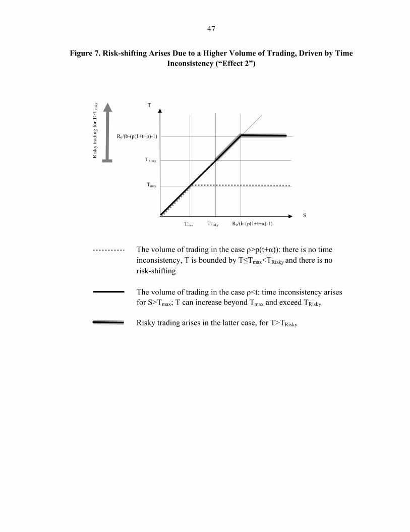
47

Figure 7. Risk-shifting Arises Due to a Higher Volume of Trading, Driven by Time Inconsistency (“Effect 2”)

T

Tmax

Tmax

TRisky

TRisky

Ris

ky tr

adin

g fo

r T

>T

Ris

ky

The volume of trading in the case ρ>p(t+α)): there is no time inconsistency, T is bounded by T≤Tmax<TRisky and there is no risk-shifting The volume of trading in the case ρ<t: time inconsistency arises for S>Tmax; T can increase beyond Tmax and exceed TRisky. Risky trading arises in the latter case, for T>TRisky

R0/(b-(p(1+t+α)-1)

R0/(b-(p(1+t+α)-1)

S