Macroeconomic Challenges Facing

Low-Income Countries

New Perspectives

January 30–31, 2014

Banking Market Structure and Macroeconomic

Stability: Are Low-Income Countries Special?

Franziska Bremus

DIW Berlin

Claudia M. Buch

Magdeburg University, Halle Institute for Economic Research, and

CESifo

Paper presented at the joint RES-SPR Conference on “Macroeconomic Challenges Facing

Low-Income Countries”

Hosted by the International Monetary Fund

With support from the UK Department of International Development (DFID)

Washington, DC—January 30–31, 2014

The views expressed in this paper are those of the author(s) only, and the presence of

them, or of links to them, on the IMF website does not imply that the IMF, its Executive

Board, or its management endorses or shares the views expressed in the paper.

1

Banking Market Structure and Macroeconomic Stability: Are Low Income Countries Special? *

Franziska Bremus

(DIW Berlin)

Claudia M. Buch

(Magdeburg University, Halle Institute for Economic Research, and CESifo)

January 2014

Abstract

The structure of banking markets in low income countries differs from developed market economies. Banking systems in lower income countries are typically smaller and less open than those in developed countries. Differences in market concentration are less stark. In this paper, we explore the channels through which the structure of banking markets affects macroeconomic volatility. We focus on granular effects: if the degree of market concentration in the banking sector is sufficiently high, idiosyncratic shocks affecting large banks can impact aggregate volatility. We find some weak evidence for granular effects in banking. However, our results suggest that a high share of domestic credit to GDP has a stronger effect on volatility in low income countries. The effects of de facto financial integration are stronger in these countries as well.

Key words: market structure, banking market integration, granular effects, macroeconomic volatility, low income countries

JEL classification: G21, E32

* Corresponding author: Franziska Bremus, German Institute for Economic Research (DIW Berlin), Mohrenstr. 58, 10117 Berlin, Germany. Phone: +49 30 89789590, Fax: +49 30 89789200, fbremus@diw.de

This paper is part of an IMF research project on macroeconomic policy in low-income countries supported by the U.K.’s Department for International Development (DFID). The views expressed in this paper are those of the author(s) and do not necessarily reflect those of DFID, the IMF, or IMF policies. The paper was written in the context of the Priority Programme SPP 1578 “Financial Market Imperfections and Macroeconomic Performance” of the German National Science Foundation (DFG). We thank Caesar Calderon and participants at the pre-conference on “Macroeconomic Challenges Facing Low income Countries”, held at the IMF on July 22-23, 2013 for helpful comments and suggestions. Hanna Schwank provided very valuable research assistance. All remaining errors and inconsistencies are our own.

2

1 Motivation

Negative effects of macroeconomic volatility on long-term growth and welfare can be

particularly pronounced in low income countries (Calderon and Yeyati 2009, Loayza et

al. 2007). Moreover, real and financial cycles are closely related (Claessens et al. 2011,

2012). One reason for the differences between high and low income countries in terms of

macroeconomic stability may thus be differences in the structure of banking systems.

Banking systems in lower income countries are typically smaller and less open than those

in developed countries.

In this paper, we explore the channels through which the structure of banking markets

affects the volatility of GDP per capita. We use a linked micro-macro panel-dataset to

show how the openness, the size, and the degree of concentration in banking markets

affect aggregate volatility. Bank-level data are taken from Bankscope. We link

macroeconomic volatility to microeconomic developments at the bank-level by drawing

on the concept of granularity (Gabaix 2011). Our results show that granular effects in

banking markets are weaker in low income countries. A higher degree of financial

integration and a higher ratio of domestic credit relative to GDP increase macroeconomic

volatility particularly in low income countries.

Our research is related to recent work which shows how heterogeneous size distributions

of firms or banks can affect macroeconomic volatility. Idiosyncratic shocks hitting

individual firms (or, in our context, banks) can affect macroeconomic volatility if the size

distribution of firms is sufficiently skewed (Gabaix 2011). If firm sizes follow a fat-tailed

power law distribution, shocks to large firms (or banks) do not cancel out across a large

number of firms as under normally distributed firm sizes. Macroeconomic volatility is

proportional to the product of volatility (or risk) at the firm-level and the Herfindahl

index of concentration. If a country’s market structure is characterized by a high degree

of concentration, i.e. if many small banks coexist with a few very large ones,

idiosyncratic shocks at the bank-level may thus be felt in the aggregate. This is in fact the

3

case in banking (Bremus et al. 2013).1 The link between bank-level and aggregate

fluctuations gets stronger as market concentration and/or idiosyncratic micro-level

volatility increase. A priori, one would thus expect granular effects – the “Banking

Granular Residual” – to be stronger in countries with a higher degree of concentration in

banking or with a higher average riskiness of the banking sector.

Comparing high and low income countries shows similar degrees of concentration

(Figure 3). Decomposing the Banking Granular Residual into its components indicates

that mean risk is higher in low than in high income countries. The degree of

concentration matters more in the high income countries. Generally, however, it is

difficult to link macroeconomic volatility to fluctuations at the bank-level as the Banking

Granular Residual and its components are mostly insignificant.

While low-income countries do not necessarily have more concentrated market structure

in banking, their banking and financial systems are less open internationally compared to

higher income countries. Recent studies find little consistent evidence on the link

between output volatility and financial openness (Kose et al. 2003, Kose et al. 2009). In

contrast, there is fairly robust evidence that greater trade openness increases output

volatility (Di Giovanni and Levchenko 2009). There are two potential reasons for the

missing link between financial integration and macroeconomic volatility, which are

particularly prevalent for low income countries. The first is that aggregated data at the

country level do not sufficiently capture heterogeneity across regions or even banks.

Loutskina and Strahan (2012) find that financial integration increases the volatility of

housing prices at the state level. Bank-level data also suggest a link between financial

market integration and the transmission of shocks across countries, which could have

implications for macroeconomic volatility. Internationally active banks use cross-border

lending to cushion the impact of domestic liquidity shocks (Cetorelli and Goldberg 2011),

and cross-border lending via local affiliates of international banks is more stable than

1 Previous work shows that granularity in banking matters for short-run output fluctuations in Eastern Europe (Buch and Neugebauer 2011), and shocks to large banks affect the probability of default of smaller banks in Germany (Blank et al. 2009). Using industry-level data, Carvalho and Gabaix (2010) show that the exposure of the macroeconomy to tail risks in the “shadow banking system” has been fairly high since the late 1990s.

4

cross-border lending at arm’s-length (De Haas and van Horen 2011). In low income

countries, which are financially less integrated, this volatility-reducing effect may be less

pronounced.

A second interpretation for the weak link between financial integration and volatility at

the aggregate level could be that threshold effects matter (Kose et al. 2011): at low levels

of institutional or financial development, financial integration may increase volatility on

financial markets. At high levels of institutional development, financial integration would

not be destabilizing. Bekaert et al. (2006) indeed find that the effects of equity market

liberalization on consumption volatility depend on a country’s state of development. This

may be due to the fact that, in countries with less developed financial markets, opening

up for foreign capital might magnify credit market friction (Aghion et al. 2004).

Consequently, both credit and output can become more volatile. Also, with limited

institutional development, capital might be allocated less than efficiently because of

corruption and crony capitalism (Johnson and Mitton 2003). The result may be a more

volatile supply of credit. These effects might be more pronounced in low than in high

income countries because of their weaker financial institutions. One proxy for financial

development that is often used in the literature is credit to GDP. Our results show a

consistently positive effect of credit to GDP on macroeconomic volatility. Instead of

proxying for financial development, this rather points to the destabilizing effects of high

leverage in an economy.

In terms of the effects of financial integration on macroeconomic volatility, we find

differences according to the measure of financial integration used. Higher de jure

openness in the sense of weaker controls on cross-border capital flows has a stabilizing

effect. Higher de facto openness, in contrast, measured through foreign assets and

liabilities relative to GDP, has a destabilizing effect in low income countries. These

differences point to the importance of managing international financial integration and

strengthening the regulatory system when opening up for foreign capital.

In the following Part 2, we describe our data. Part 3 presents the regression model and the

results, while Part 4 concludes.

5

2 Data and Measurement of Volatility

2.1 Macroeconomic Data

The macroeconomic data used in this paper are taken from the World Development

Indicators (WDI) by the World Bank. Details on the measurement and the data sources

are given in Appendix A.

We start from a dataset which includes a large set of countries, and we keep those with

complete strings of observations of at least ten years for key variables, including GDP per

capita growth, foreign assets and liabilities, and domestic credit relative to GDP. This

sample includes 97 countries for 14 years (1998-2011). Due to the unbalanced nature of

the panel, the maximum number of country-year observations is 972 if we include control

variables. Table 1 shows descriptive statistics for the baseline regression sample.

Our country sample includes 15 low income countries (as classified by the IMF). These

are Bangladesh, Bolivia, Cote d’Ivoire, Georgia, Ghana, Kenya, Kygrgyz Republic,

Malawi, Mongolia, Nepal, Nigeria, Tanzania, Uganda, Vietnam, and Zambia. In terms of

macroeconomic data, we could use a larger country sample, but the binding constraint is

finding low income countries with a sufficiently large number of individual bank

observations. In Bankscope, we have bank data for more than these 15 low income

countries, but the number of banks for many of the low income countries are less than 5

per year.

2.2 Banking Market Integration

To measure banking market integration, we use a de facto and a de jure measure. Our de

facto measure is taken from an updated and extended version of the external wealth

dataset constructed by Lane and Milesi-Ferretti (2007), which is available for the period

1970-2011. In the international trade literature, the degree of trade openness is often

measured as the sum of imports and exports relative to GDP. In line with this, we use the

sum of foreign assets and foreign liabilities relative to GDP as a proxy for de facto

financial integration.

6

Information on capital controls comes from Chinn and Ito (2006, 2008). These authors

use the IMF’s Annual Report on Exchange Restrictions and Regulations to construct a

measure of capital controls. We use their data as a de jure measure of financial

integration. The Chinn-Ito index is based on dummy variables which codify restrictions

on cross-border financial transactions. The minimum number is -1.82 (financially closed),

the maximum number is 2.46 (financially open). Hence, financial openness measures are

both scaled such that a higher number indicates a more open financial system.

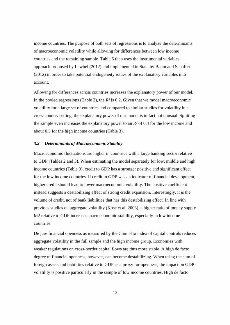
The second panel of Figure 3 shows our measures of de facto and de jure openness.

Poorer countries are generally much less financially open than high income countries.

Because results from previous studies suggest that granular effects are stronger in

financially closed economies (Bremus and Buch 2013), this could suggest that granular

effects are stronger in low income countries.

2.3 Banking Market Structure

We use two main measures of the structure of banking markets – the size of banking

systems and the degree of concentration of banks’ assets. The size of banking markets is

measured as the share of domestic credit to the private sector relative to GDP. Previous

literature has often interpreted the share of credit over GDP as a measure for financial

development. Yet, credit over GDP is also a measure for the degree of leverage in an

economy.

Figure 3 shows that domestic credit to GDP is much lower in low than in high income

countries. The expected impact of credit over GDP on macroeconomic volatility is not

clear a priori: the more financially developed a country is, the lower should be the

volatility of macroeconomic aggregates. The higher credit, in contrast, the higher would

we expect volatility to be for a given shock because higher credit implies larger multiplier

effects. Moreover, if institutions and regulation are weak, credit may be allocated less

efficiently which may harm macroeconomic stability.

In order to control for the importance of equity markets, we include stock market

capitalization of listed companies (in percent of GDP) in our regressions. The data come

from the World Development Indicators. Market capitalization of listed companies to

7

GDP is much lower in low income countries than in higher-income economies. This may

be interpreted again as low financial market development – not only in banking but also

in the equity market – in low income countries.

The concentration of banking markets, i.e. the dispersion of assets across banks, is

measured through the banking system’s Herfindahl index (HHI). The underlying data are

taken from Bankscope. The HHI is computed as the sum of banks’ squared market shares

for each country and year. We use this measure of concentration, because we want to

study granular effects and our theoretically founded measure of granularity includes the

Herfindahl index.

Figure 3 reveals that banking market concentration measured by the Herfindahl index of

bank loans or assets has followed a downward trend in our sample across all income

groups. The Herfindahl index tends to be higher in the most developed economies, which

may point to a larger role of granular effects for macroeconomic stability for this group of

countries.

2.4 Bank-Level Data

Our source for bank-level data is Bankscope, a commercial database provided by Bureau

van Dijck, which provides income statements and balance sheets for banks worldwide. A

number of screens are imposed on the banking data in order to eliminate errors due to

misreporting. We exclude the bottom 1% of the observations for total assets, and we drop

observations where the loans-to-assets or the equity-to-assets ratio is larger than one as

well as banks with negative equity, assets, or loans. In order to eliminate large (absolute)

growth rates that might be due to bank mergers, we winsorize growth rates at the top or

bottom percentile, i.e. the growth rates are replaced with the respective percentiles. In

terms of specializations of banks, we keep bank holding companies, commercial banks,

cooperative banks, and savings banks.

2.5 Measuring Volatility

The dependent variable of interest is the volatility of GDP per capita. Many previous

studies use the standard deviation of GDP growth rates as a measure of (aggregate)

volatility, where the standard deviation is calculated over a certain window of

8

observations of five or ten years. The disadvantage of this method is that the choice of the

time window is somewhat arbitrary and, perhaps more importantly, that the dependent

variable is auto-correlated by construction. This autocorrelation needs to be taken into

account when estimating the determinants of volatility by, for instance, estimating a

dynamic panel model. Yet, dynamic panel models are sensitive to the choice of the

instruments.

For these reasons, we resort to a simple alternative measure of volatility, which has been

used in recent work by Loutskina and Strahan (2012) and Kalemli-Ozcan et al. (2010).

To calculate the volatility of house prices, Loutskina and Strahan (2012) use the absolute

deviation of house price growth after removing time and regional fixed effects. Applying

their methodology, we can retrieve the volatility of real GDP per capita growth from the

following regression

ln GDP , ‐ ln GDP , ‐ Δ ln GDP , α γ GDPShock , (1)

where and are time- and country-fixed effects, respectively. The volatility of GDP

growth is given by , , , i.e. by the absolute value of the

regression residual. In order to prevent large outliers from affecting the results, large

growth rates in the top and bottom percentile are winsorized.

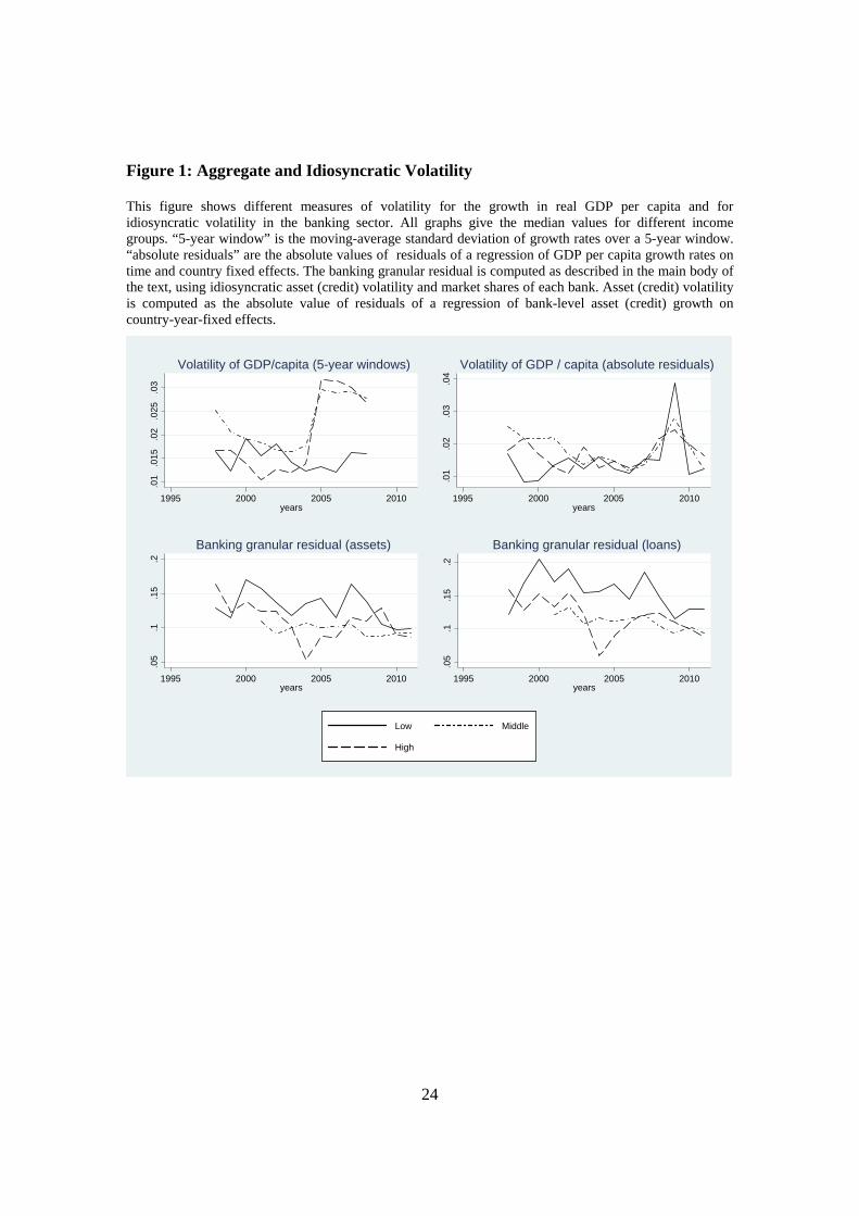
Figure 1 shows that macroeconomic volatility, measured by absolute residuals, has

increased across all income groups during the global financial crisis and has subsequently

fallen again.

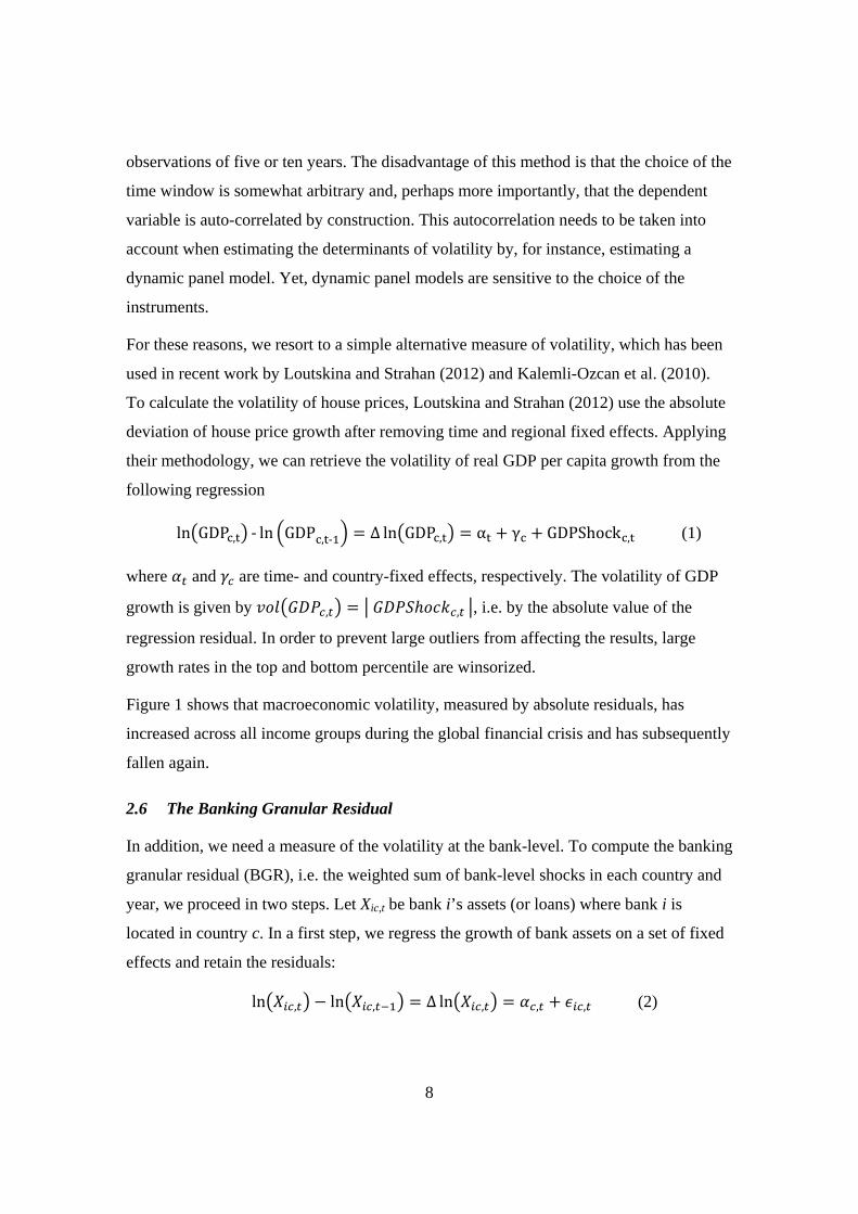
2.6 The Banking Granular Residual

In addition, we need a measure of the volatility at the bank-level. To compute the banking

granular residual (BGR), i.e. the weighted sum of bank-level shocks in each country and

year, we proceed in two steps. Let Xic,t be bank i’s assets (or loans) where bank i is

located in country c. In a first step, we regress the growth of bank assets on a set of fixed

effects and retain the residuals:

ln , ln , Δ ln , , , (2)

9

where , are country-year fixed effects and Δ ln , is the log growth rate of bank i’s

assets. The residual of equation (2) is a measure for idiosyncratic shocks at the bank-

level, which is purged from macroeconomic and common banking factors.

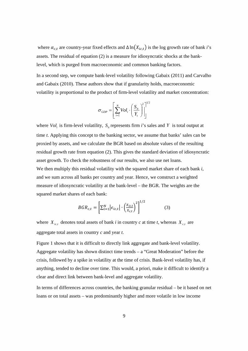
In a second step, we compute bank-level volatility following Gabaix (2011) and Carvalho

and Gabaix (2010). These authors show that if granularity holds, macroeconomic

volatility is proportional to the product of firm-level volatility and market concentration:

21

1

2

N

i t

itiGDP Y

SVol

where iVol is firm-level volatility, itS represents firm i’s sales and is total output at

time t. Applying this concept to the banking sector, we assume that banks’ sales can be

proxied by assets, and we calculate the BGR based on absolute values of the resulting

residual growth rate from equation (2). This gives the standard deviation of idiosyncratic

asset growth. To check the robustness of our results, we also use net loans.

We then multiply this residual volatility with the squared market share of each bank i,

and we sum across all banks per country and year. Hence, we construct a weighted

measure of idiosyncratic volatility at the bank-level – the BGR. The weights are the

squared market shares of each bank:

, ∑ , ∙ ,

,

/

(3)

where ticX , denotes total assets of bank i in country c at time t, whereas tcX , are

aggregate total assets in country c and year t.

Figure 1 shows that it is difficult to directly link aggregate and bank-level volatility.

Aggregate volatility has shown distinct time trends – a “Great Moderation” before the

crisis, followed by a spike in volatility at the time of crisis. Bank-level volatility has, if

anything, tended to decline over time. This would, a priori, make it difficult to identify a

clear and direct link between bank-level and aggregate volatility.

In terms of differences across countries, the banking granular residual – be it based on net

loans or on total assets – was predominantly higher and more volatile in low income

Y

10

countries across our sample period (Figure 1). After the crisis, the BGR tended to

decrease across all income groups.

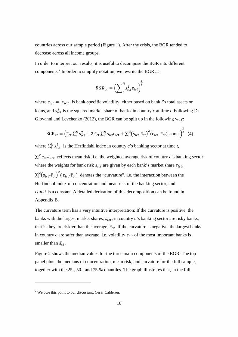
In order to interpret our results, it is useful to decompose the BGR into different

components.2 In order to simplify notation, we rewrite the BGR as

where , is bank-specific volatility, either based on bank i’s total assets or

loans, and is the squared market share of bank i in country c at time t. Following Di

Giovanni and Levchenko (2012), the BGR can be split up in the following way:

BGR ε ∑ s 2s ∑ s ε ∑ s ‐s ε ‐ ε ‐const (4)

where ∑ is the Herfindahl index in country c’s banking sector at time t,

∑ reflects mean risk, i.e. the weighted average risk of country c’s banking sector

where the weights for bank risk are given by each bank’s market share ,

∑ s ‐s ε ‐ε denotes the “curvature”, i.e. the interaction between the

Herfindahl index of concentration and mean risk of the banking sector, and

is a constant. A detailed derivation of this decomposition can be found in

Appendix B.

The curvature term has a very intuitive interpretation: If the curvature is positive, the

banks with the largest market shares, , in country c’s banking sector are risky banks,

that is they are riskier than the average, . If the curvature is negative, the largest banks

in country c are safer than average, i.e. volatility of the most important banks is

smaller than .

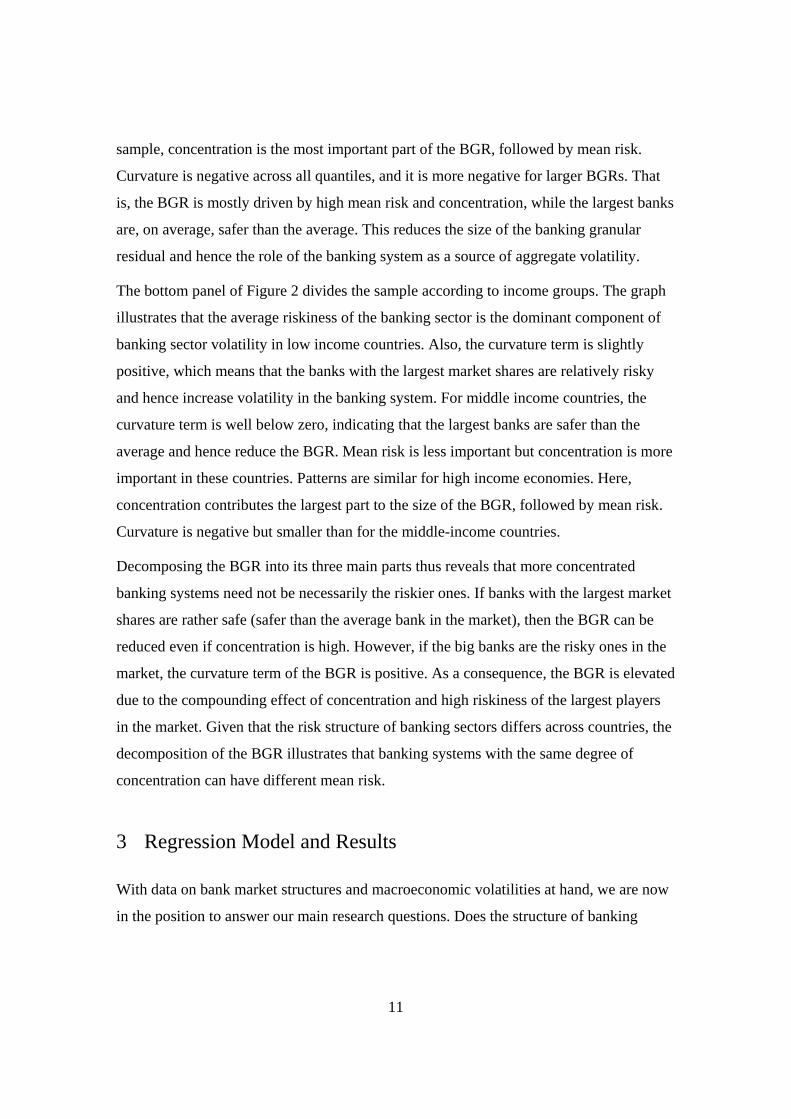
Figure 2 shows the median values for the three main components of the BGR. The top

panel plots the medians of concentration, mean risk, and curvature for the full sample,

together with the 25-, 50-, and 75-% quantiles. The graph illustrates that, in the full

2 We owe this point to our discussant, César Calderón.

11

sample, concentration is the most important part of the BGR, followed by mean risk.

Curvature is negative across all quantiles, and it is more negative for larger BGRs. That

is, the BGR is mostly driven by high mean risk and concentration, while the largest banks

are, on average, safer than the average. This reduces the size of the banking granular

residual and hence the role of the banking system as a source of aggregate volatility.

The bottom panel of Figure 2 divides the sample according to income groups. The graph

illustrates that the average riskiness of the banking sector is the dominant component of

banking sector volatility in low income countries. Also, the curvature term is slightly

positive, which means that the banks with the largest market shares are relatively risky

and hence increase volatility in the banking system. For middle income countries, the

curvature term is well below zero, indicating that the largest banks are safer than the

average and hence reduce the BGR. Mean risk is less important but concentration is more

important in these countries. Patterns are similar for high income economies. Here,

concentration contributes the largest part to the size of the BGR, followed by mean risk.

Curvature is negative but smaller than for the middle-income countries.

Decomposing the BGR into its three main parts thus reveals that more concentrated

banking systems need not be necessarily the riskier ones. If banks with the largest market

shares are rather safe (safer than the average bank in the market), then the BGR can be

reduced even if concentration is high. However, if the big banks are the risky ones in the

market, the curvature term of the BGR is positive. As a consequence, the BGR is elevated

due to the compounding effect of concentration and high riskiness of the largest players

in the market. Given that the risk structure of banking sectors differs across countries, the

decomposition of the BGR illustrates that banking systems with the same degree of

concentration can have different mean risk.

3 Regression Model and Results

With data on bank market structures and macroeconomic volatilities at hand, we are now

in the position to answer our main research questions. Does the structure of banking

12

markets affect macroeconomic volatility and, if yes, is this link different in low income

countries?

3.1 Empirical Model

As a baseline setup, we regress macroeconomic volatility on the BGR and its first lag, on

financial market integration and on variables measuring financial market structures.

Hence, we estimate the following equation:

Vol , α γ β BGR , β BGR , ‐ β,

β MCap , β FI , ϵ ,

where , is GDP-volatility, is a vector of year fixed effects capturing global

macroeconomic factors, are country fixed effects, , is the banking granular

residual, ,

is the ratio of bank credit over GDP, , measures market

capitalization of listed companies (in % of GDP), and tcFI , includes de facto and de jure

financial market integration.

Second, we use the mean risk and the Herfindahl index of concentration as individual

regressors instead of the BGR, so that the regression model becomes

, , , ,,

, , ,

where is mean risk computed as the weighted average of bank-level volatility, the

weights being each bank’s market share. Mean risk is closely related to the Granular

Residual in growth regressions such as used by Gabaix (2011) or Bremus et al. (2013).

Table 1 shows descriptive statistics for the regression sample, while Table 2 presents the

results for our baseline regressions (Columns 1 and 2) using the volatility of GDP per

capita growth as the dependent variable. In Columns 3 and 4 of Table 2, we add

additional explanatory variables which are standard controls in the literature on

macroeconomic volatility. In Table 3, we run the regressions for different income groups

separately. Table 4 shows similar regressions for the full country sample, but including

interaction terms between the explanatory variables and a dummy variable for low

13

income countries. The purpose of both sets of regressions is to analyze the determinants

of macroeconomic volatility while allowing for differences between low income

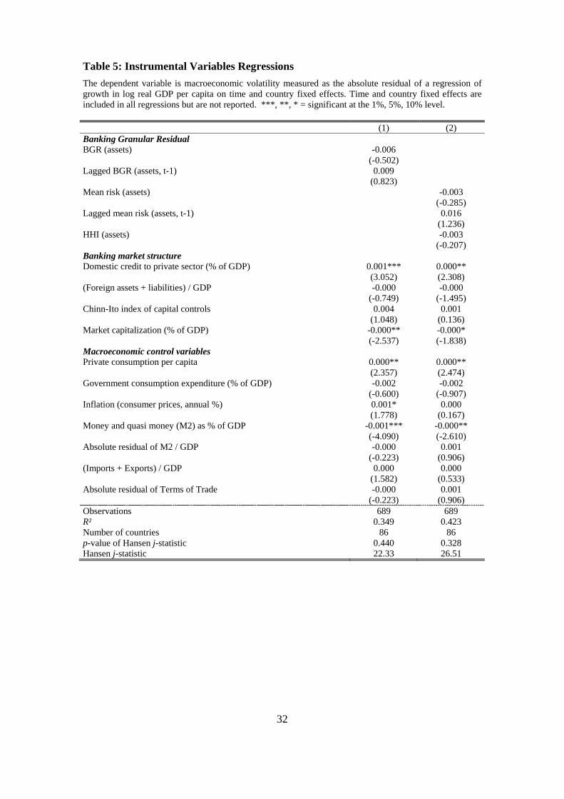
countries and the remaining sample. Table 5 then uses the instrumental variables

approach proposed by Lewbel (2012) and implemented in Stata by Baum and Schaffer

(2012) in order to take potential endogeneity issues of the explanatory variables into

account.

Allowing for differences across countries increases the explanatory power of our model.

In the pooled regressions (Table 2), the R² is 0.2. Given that we model macroeconomic

volatility for a large set of countries and compared to similar studies for volatility in a

cross-country setting, the explanatory power of our model is in fact not unusual. Splitting

the sample even increases the explanatory power to an R² of 0.4 for the low income and

about 0.3 for the high income countries (Table 3).

3.2 Determinants of Macroeconomic Stability

Macroeconomic fluctuations are higher in countries with a large banking sector relative

to GDP (Tables 2 and 3). When estimating the model separately for low, middle and high

income countries (Table 3), credit to GDP has a stronger positive and significant effect

for the low income countries. If credit to GDP was an indicator of financial development,

higher credit should lead to lower macroeconomic volatility. The positive coefficient

instead suggests a destabilizing effect of strong credit expansion. Interestingly, it is the

volume of credit, not of bank liabilities that has this destabilizing effect. In line with

previous studies on aggregate volatility (Kose et al. 2003), a higher ratio of money supply

M2 relative to GDP increases macroeconomic stability, especially in low income

countries.

De jure financial openness as measured by the Chinn-Ito index of capital controls reduces

aggregate volatility in the full sample and the high income group. Economies with

weaker regulations on cross-border capital flows are thus more stable. A high de facto

degree of financial openness, however, can become destabilizing. When using the sum of

foreign assets and liabilities relative to GDP as a proxy for openness, the impact on GDP-

volatility is positive particularly in the sample of low income countries. High de facto

14

openness does not significantly affect macroeconomic stability in the richer economies

though.

The different effects of de facto financial openness on macroeconomic stability in low

and in higher income countries are consistent with the observation that institutional

quality is poorer and financial development is lower in low income countries (Kose et al.

2011, Bekaert et al. 2006). As a consequence, capital is used less efficiently in low

income countries, so that higher cross-border assets and liabilities relative to GDP can be

destabilizing in low income countries.

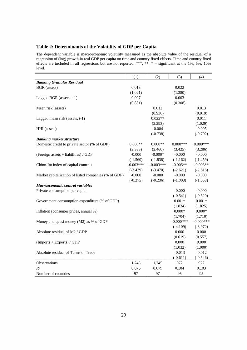
The Banking Granular Residual does not significantly impact aggregate stability in the

full set of countries (Table 2, Columns 1 and 3). When including mean risk and

concentration separately (Columns 2 and 4), results show that countries with a higher

average riskiness of the banking system experience higher aggregate volatility. In low

income countries, the BGR has a contemporaneously negative and a lagged positive

impact on GDP volatility (Table 3). Concentration as measured by the Herfindahl index

does not have a significant impact on macroeconomic stability.

When including interaction terms for low income countries (Table 4), the effects of most

explanatory variables remain the same as in the baseline setup. The direct effect of the

BGR turns positive and significant if an interaction with a low income dummy is added to

the model. The interaction term itself is negative, i.e. granular effects from banking are

weaker and even negative in low income countries. Put differently, higher banking sector

risk would reduce rather than increase aggregate volatility low income countries, as

would be expected from theory. However, these results are based on a relatively small

country sample and may thus not be robust to changes in the selection of countries. In

future work, it would be interesting to explore whether the co-movement of banking

sector risk and other risk factors in the economy might drive this result.

Considering mean risk and concentration as separate regressors, the effect of mean

banking sector risk is negative in low income economies. However, the interaction term

between the low-income dummy and the Herfindahl index is positive. Hence, there is a

volatility-enhancing effect of concentration in low income countries but not in the

remaining country sample.

15

3.3 Robustness Tests

In order to test the robustness of our results, we have run several alternative regressions.

First, we have used the BGR and its components based on net loans instead of assets as

an alternative specification of banking sector volatility.3 The results remain broadly the

same, but the BGR based on assets has stronger significant effects than the BGR based on

net loans.

Second, we interact all variables of interest with a banking crisis dummy which is

available from Laeven and Valencia (2012). Again, the results remain broadly

unchanged. The effect of the Herfindahl index on GDP-volatility turns negative when

including an interaction with the crisis-dummy. As expected, volatility is higher in times

of crisis. Hence, higher banking sector concentration increases volatility in crisis times

while it stabilizes output in normal times.

Finally, Table 5 presents results for instrumental variables regressions. Even though the

BGR is exogenous by construction, other determinants of macroeconomic stability may

be endogenous. For example, domestic credit may drop due to a decline in credit demand

during bad times, or financial markets may close down in periods of high macroeconomic

instability.

We use the third lag of domestic credit to GDP, de facto and de jure financial openness,

trade openness, market capitalization, M2 to GDP, the volatility of the terms of trade

index, and government and private consumption to GDP as instruments. For inflation and

the volatility of M2 to GDP, we use the first lag, because the second and third lags are not

significant in the first stage regressions. In order to increase efficiency of the instrumental

variable regressions, we employ the methodology proposed by Lewbel (2012). This

approach allows constructing additional instruments as simple functions of the regressors.

The results support our previous findings that high credit to GDP and high inflation

increase macroeconomic instability. High market capitalization and high M2 to GDP

decrease instability. When instrumenting the regressors, we find positive and significant

3 The regression results are available from the authors upon request.

16

effects of the volatility of the terms of trade and of M2 to GDP, consistent with previous

literature. Moreover, a higher ratio of private consumption to GDP increases aggregate

volatility. Trade openness remains insignificant in our regression sample.

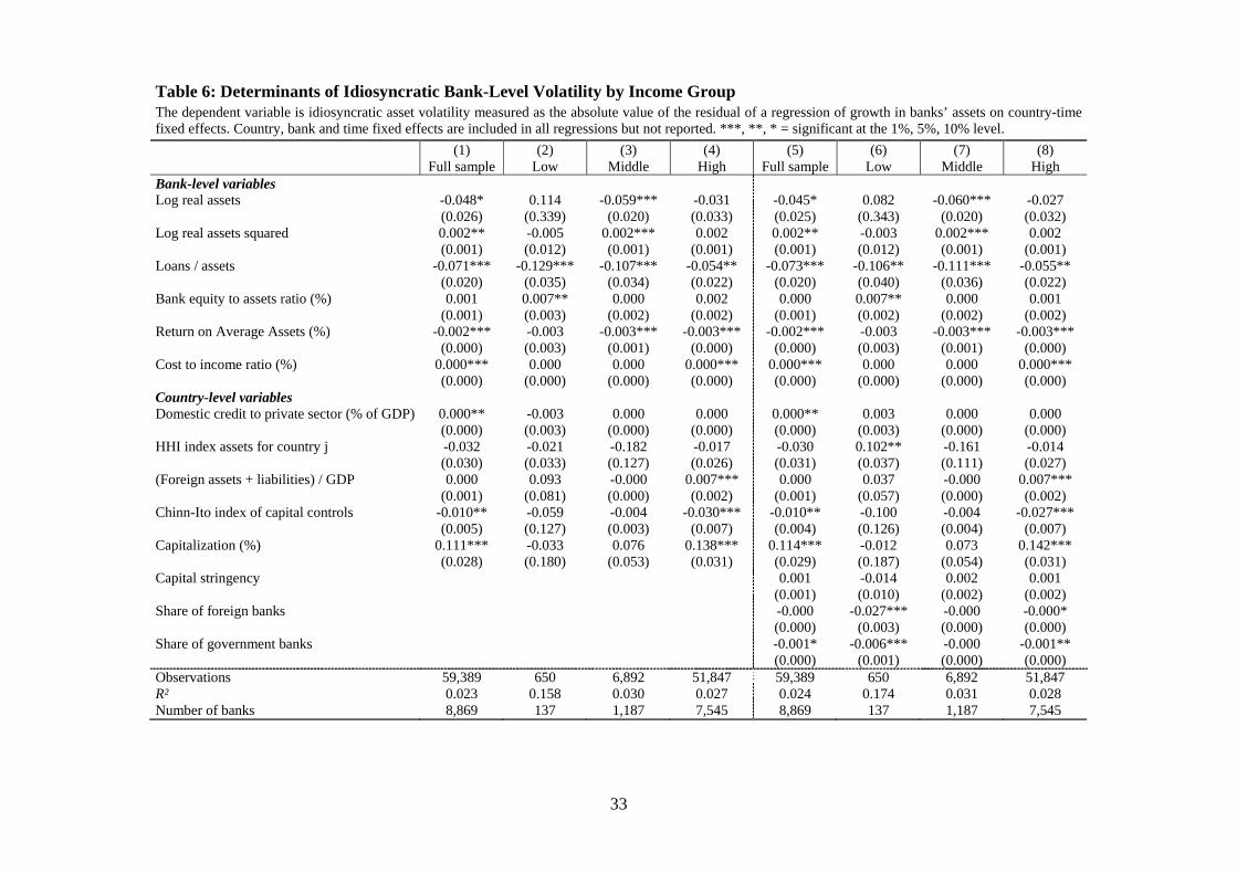
3.4 Determinants of Idiosyncratic Bank-Level Risk

So far, we have shown that the banking granular residual and average idiosyncratic risk in

banking affect macroeconomic outcomes. Now, we go one step further and analyze the

factors driving one important component of the BGR, namely bank-level idiosyncratic

risk.

Table 6 shows regression results for the idiosyncratic volatility of asset growth of banks

as the dependent variable. We run separate regressions for the whole sample, for low,

middle, and high income countries. Bank-, country- and year-fixed effects are included in

each regression.

With respect to individual bank characteristics, idiosyncratic volatility decreases in the

share of banks’ loans relative to their total assets. In this sense, banks performing core

intermediation functions are less risky. Banks with a higher equity capital buffer have

more volatile asset growth, but this effect is reminiscent of the low income countries only

(Table 6, Columns 2 and 6). This result may actually be due to reversed causality: banks

with riskier loans may need higher capital buffers to insure against the resulting risks.

The link between bank size and risk is not clear, a priori. On the one hand, larger banks

should be more diversified and have better screening models. Both should make them

less risky. On the other hand, larger banks enjoy a too big to fail subsidy, which increases

their risk-taking incentives. Here, our results differ across income groups. In middle

income countries, larger banks tend to have less volatile credit but this effect levels off if

bank size gets very high. For banks in low and in high income countries, bank size does

not matter for idiosyncratic fluctuations. The return on average assets reduces bank-level

risk in all but in the low income countries, while a higher cost to income ratio and hence

lower efficiency increases bank risk in high income countries.

In these models, we also control for structural features of the banking markets. A high

level of credit to GDP increases bank-level volatility in the whole sample. This is

17

consistent with results at the aggregate level. Credit to GDP is insignificant in the sample

splits according to income groups. De jure financial openness tends to reduce bank-level

fluctuations in high-income countries, while it has no significant impact on bank risk in

low and middle income economies. Banking sector capitalization, i.e. the capital to asset

ratio at the aggregate level, leads to higher bank risk in rich countries. Finally, asset

growth gets less volatile with higher shares of foreign banks and higher shares of

government banks especially in low income countries.

4 Summary

In this paper, we study the impact of banking market structure on macroeconomic

volatility. We particularly focus on low income countries. Compared to higher income

countries, low income countries are characterized by higher banking sector risk, lower

degrees of international integration, and smaller overall banking systems. The degree of

concentration is similar. Our study has three main findings.

First, idiosyncratic risk at the bank level has no strong impact on macroeconomic

volatility. Yet, decomposing the Banking Granular Residual into its components shows

that a high degree of concentration in banking markets increases aggregate volatility in

low income countries.

Second, at the aggregate level, a higher ratio of bank credit relative to GDP increases

macroeconomic volatility in particular in low income countries. At the micro-level,

however, domestic credit does not matter much for volatility in low income countries.

Third, increased financial integration is a double-edged sword. Reducing capital controls

– and thus a higher degree of de jure openness – has a stabilizing effect. High ratios of

foreign assets and liabilities over GDP increase GDP volatility in low income countries,

in contrast.

In terms of policy implications, our results imply that there are different channels through

which macroeconomic volatility can be reduced: by limiting the excessive expansion of

credit in an economy, by reducing idiosyncratic and thus bank-level volatility, and by

reducing the degree of concentration. We have also shown that the impact of financial

18

openness on macroeconomic volatility depends on the openness measure chosen. It

would be an interesting avenue for future work to analyze whether these findings are

driven by the quality of banking regulations across countries.

19

5 References

Aghion, P., P. Bacchetta, and A. Banerjee (2004). Financial development and the instability of open economies. Journal of Monetary Economics 51(6): 1077-1106.

Baum, C. and Schaffer (2012). IVREG2H: Stata module to perform instrumental variables estimation using heteroskedasticity-based instruments, Statistical Software Components, Boston College, Department of Economics.

Beck, T., A. Demirgüç-Kunt, and R. Levine (2000). A New Database on Financial Development and Structure. World Bank Economic Review 14: 597-605.

Beck, T., and A. Demirgüç-Kunt (2009). Financial Institutions and Markets Across Countries and over Time: Data and Analysis. World Bank Policy Research Working Paper 4943. Washington D.C.

Bekaert, G., C.R. Harvey, and C. Lundblad (2006). Growth volatility and financial liberalization. Journal of International Money and Finance 25: 370-403.

Blank, S., C.M. Buch, and K. Neugebauer (2009). Shocks at large banks and banking sector distress: The Banking Granular Residual. Journal of Financial Stability 5(4): 353-373.

Bremus, F., and C.M. Buch (2013). Granularity in Banking and Growth: Does Financial Openness Matter?, CESifo Working Paper Series 4356, CESifo Group Munich.

Bremus, F., C.M. Buch, K.N. Russ, and M. Schnitzer (2013). Big Banks and Macroeconomic Outcomes Theory and Cross-Country Evidence of Granularity, NBER Working Paper 19093. Cambridge, MA.

Buch, C.M., and K. Neugebauer (2011). Bank-specific shocks and the real economy. Journal of Banking and Finance 35(8): 2179-2187.

Calderon, C., and E.L. Yeyati (2009). Zooming in: from aggregate volatility to income distribution, Policy Research Working Paper Series 4895, The World Bank.

Carvalho, V.M., and X. Gabaix (2010). The Great Diversification and its Undoing. NBER Working Paper No. 16424. Cambridge, MA.

Cetorelli, N., and L. Goldberg (2011). Global banks and international shock transmission: Evidence from the crisis. IMF Economic Review 59: 41-76.

Chinn, M.D., and H. Ito (2006). What Matters for Financial Development? Capital Controls, Institutions, and Interactions. Journal of Development Economics 81(1): 163-192.

Chinn, M.D., and H. Ito (2008). A New Measure of Financial Openness. Journal of Comparative Policy Analysis 10(3): 309 – 322.

Claessens, S. and N. van Horen (2013). Foreign banks: Trends and Impact. Journal of Money, Credit, and Banking, forthcoming.

20

Claessens, S., M.A. Kose, and M.E. Terrones (2011). “Recessions and Financial Disruptions in Emerging Markets: A Bird’s Eye View. In: Cespedes, L., R. Chang, and D. Saravia (eds.) Monetary Policy Under Financial Turbulence, Central Bank of Chile.

Claessens, S., M.A. Kose, and M.E. Terrones, (2012). How do business and financial cycles interact?, Journal of International Economics 87(1): 178-190.

De Haas, R., and N. van Horen (2011). Running for the exit: international banks and crisis transmission. EBRD Working Paper 124. London.

Di Giovanni, J., and A.A. Levchenko (2009). Trade Openness and Volatility, Review of Economics and Statistics 91(3): 558-585.

Di Giovanni, J., A.A. Levchenko, and R. Rancière (2012). The Risk Content of Exports: A Portfolio View of International Trade, NBER International Seminar on Macroeconomics, University of Chicago Press 8(1): 97 - 151.

Gabaix, X. (2011). The Granular Origins of Aggregate Fluctuations. Econometrica 79(3): 733-772.

Johnson, S. and T. Mitton (2003). Cronyism and capital controls: Evidence from Malaysia. Journal of Financial Economics 67(2): 351-382.

Kalemli-Ozcan, S., B.E. Sørensen, and V. Volosovych (2010). Deep Financial Integration and Volatility. NBER Working Papers 15900. National Bureau of Economic Research. Cambridge, MA.

Kose, M.A., E. Prasad, K. Rogoff, and S.-J. Wei (2009). Financial Globalization: A Reappraisal. IMF Staff Papers 56(1): 8-62.

Kose, M.A., E.S. Prasad, and A.D. Taylor (2011). Threshold Effects in the Process of International Financial Integration. Journal of International Money and Finance 30(1):147-179.

Kose, M.A., E.S. Prasad, and M.E. Terrones (2003). Financial Integration and Macroeconomic Volatility. IMF Working Paper No. 03/50. Washington D.C.

Laeven, L. and F. Valencia (2012). Systemic Banking Crises Database: An Update, IMF Working Paper No. 12/163. Washington, D.C.

Lane, P.R., and G.M. Milesi-Ferretti (2007). The External Wealth of Nations Mark II. Journal of International Economics 73: 223-250.

Lewbel (2012). Using Heteroscedasticity to Identify and Estimate Mismeasured and Endogenous Regressor Models, Journal of Business and Economic Statistics 30(1): 67-80.

Loayza, N.V., R. Rancière, L. Servén, and J. Ventura (2007). Macroeconomic Volatility and Welfare in Developing Countries: An Introduction, World Bank Economic Review 21(3): 343 – 357.

Loutskina, E., P.E. Strahan (2012). Financial Integration, Housing and Economic Volatility. University of Virginia and Boston College. Mimeo, available at http://ssrn.com/abstract=1991430.

21

Appendix A: Data Definition and Sources

Income groups: The group of low income countries follows the classification of the Poverty Reduction and Growth Trust (PRGT)-eligible countries from the IMF/WEO. The group of middle income countries includes countries which are classified as middle income countries by the World Bank, but without PRGT-eligible countries. High-income countries are classified according to the World Bank.

List of countries (PRGT-eligible countries are in italics): Argentina, Armenia, Australia, Austria, Bahrain, Bangladesh, Belgium, Bolivia, Botswana, Brazil, Bulgaria, Canada, Chile, China, Colombia, Costa Rica, Cote d'Ivoire, Croatia , Cyprus, Czech Republic, Denmark, Ecuador, Egypt, El Salvador, Estonia, Finland, France, Georgia, Germany, Ghana, Greece, Hong Kong, China, Hungary, India, Indonesia, Ireland, Israel, Italy, Japan, Jordan, Kazakhstan, Kenya, Korea. Rep., Kuwait, Kyrgyz Republic, Latvia, Lebanon, Lithuania, Macedonia, Malawi, Malaysia, Malta, Mauritius, Mexico, Mongolia, Morocco, Namibia, Nepal, Netherlands, New Zealand, Nigeria, Norway, Oman, Pakistan, Panama, Paraguay, Peru, Philippines, Poland, Portugal, Qatar, Romania, Russian Federation, Saudi Arabia, Singapore, Slovak Republic, Slovenia, South Africa, Spain, Swaziland, Sweden, Switzerland, Tanzania, Thailand, Trinidad and Tobago, Tunisia, Turkey, Uganda, Ukraine, United Arab Emirates, United Kingdom, United States, Uruguay, Venezuela, Vietnam, Zambia.

Banking granular residual: To compute the banking granular residual as described in the text, we use bank-level data on total net loans and total assets from the Bankscope database for the period 1997-2011. In Bankscope, we keep observations with the consolidation codes C1 (consolidated and companion is not on the disc), C2 (consolidated and companion is on the disc), U1 (unconsolidated and companion is not on the disc or the bank does not publish consolidated accounts), and A1 (aggregated statements with no companion), so that double-countings are eliminated.

Bank-level volatility: Computed as the absolute residual of a regression of bank-level assets (loan) growth on country-year-fixed effects using the Bankscope dataset.

Bank size: We measure bank size by the logarithm of each bank’s total assets (loans) using information from Bankscope.

Bank equity / assets (%): Total bank equity and assets are available from Bankscope for the period 1997-2011.

Capital controls: We use the Chinn-Ito index as a de jure measure for financial openness. This variable measures a country’s degree of capital account openness and is available for the period 1970-2011 and 182 countries. It ranges from -1.82 to 2.46 with a sample mean of zero. The smaller the Chinn-Ito Index, the lower (de jure) financial openness.

Capitalization: We measure capitalization as the ratio of banking sector capital to total assets. The data are available at annual frequency from the WDI.

Capital regulation stringency index: Data on the stringency of capital regulation is available from Barth et al. (2013) for 1999, 2002, 2006 and 2011. We assign the information for 1999 to the period 1998 – 2001, 2002 to 2002 – 2005, 2006 to 2006-2009 and 2011 to the period 2010 -2011.

22

Concentration: As a measure of concentration in the banking sector, we compute Herfindahl-indexes for each country and year based on net loans and assets from Bankscope.

Cost / income: The ratio of banks’ operating costs relative to income (in %) is retrieved from Bankscope.

Credit to GDP: Credit to the private sector in percent of GDP is taken from the WDI.

GDP per capita growth: We compute growth as the log-difference in constant 2005 US-Dollars. The data on GDP per capita come from the WDI.

Government consumption expenditure / GDP: Data on general government final consumption expenditure in percent of GDP (in constant 2005 USD) is taken from the WDI.

Inflation (consumer prices, annual %): WDI.

Loans / assets: Each banks’ total netloans relative to total assets are computed using data from Bankscope.

Market capitalization of listed companies (% of GDP): The data is taken from the WDI.

Mean banking sector risk: We compute mean risk as the weighted sum of the absolute value of idiosyncratic, bank-level asset (loan) growth, where the weights are given by each bank’s market share (see equation (4) in the main text).

M2 / GDP: Money and quasi money (M2) relative to GDP is retrieved from the WDI.

Real private consumption per capita (USD): Data on real private consumption and on total population come from the WDI.

Return on average assets (ROAA): The return of average assets (%) is available from Bankscope.

Share of foreign-owned banks (%): The information is available from Barth et al. (2013). Timing is set as for the capital stringency index.

Share of government-owned banks (%): The information is available from Barth et al. (2013). Timing is set as for the capital stringency index.

Total foreign assets and liabilities relative to GDP: We use data on total foreign assets and liabilities in US-Dollars from the updated database by Lane and Milesi-Feretti (2007) which is available for the period 1970-2011 for 178 countries. GDP-data is taken from the WDI.

Trade openness: We take exports and imports relative to GDP from the WDI.

Volatility of M2 / GDP: We compute absolute residuals from a regression of M2 / GDP on country- and time-fixed effects.

Volatility of Terms of Trade: Absolute residuals are computed from a regression of the terms of trade index (available from the WDI) on country and time fixed effects (see equation (2) in the main text).

23

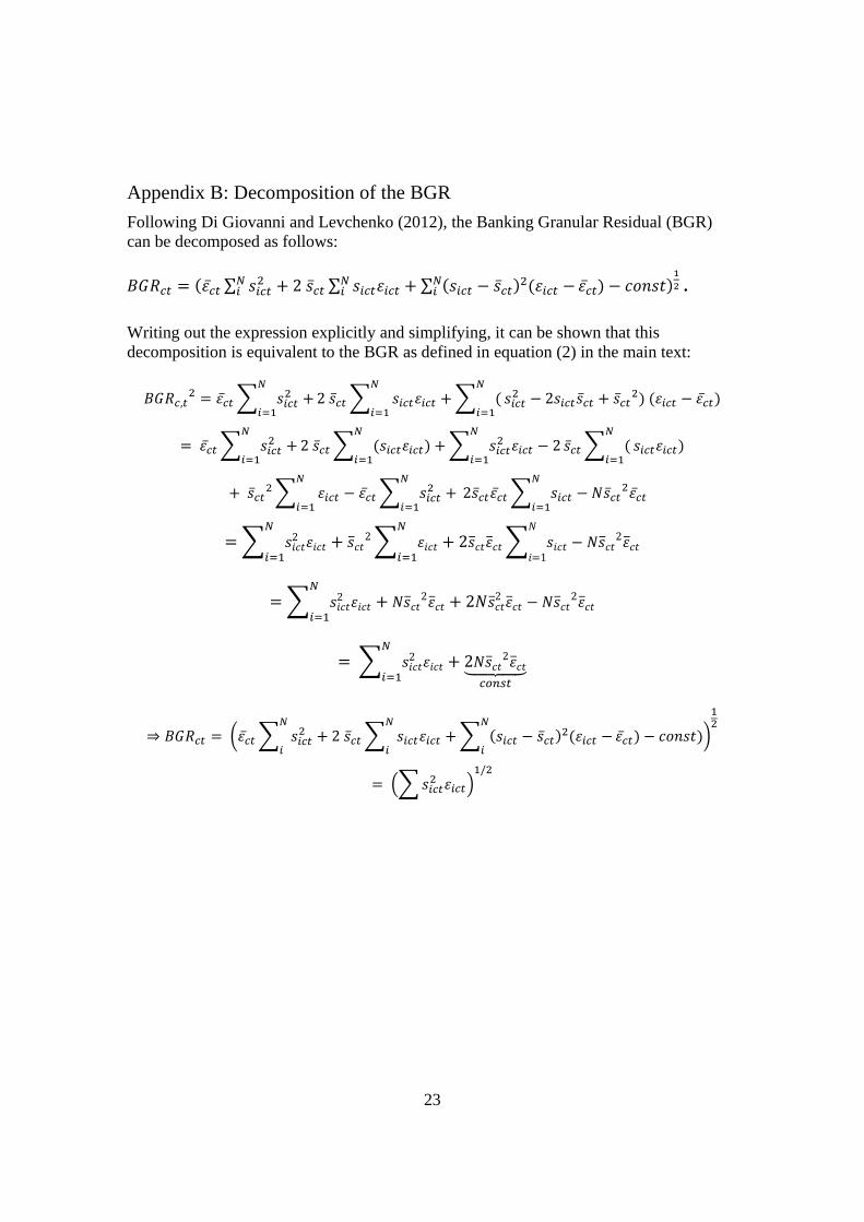
Appendix B: Decomposition of the BGR

Following Di Giovanni and Levchenko (2012), the Banking Granular Residual (BGR) can be decomposed as follows:

∑ 2 ∑ ∑ .

Writing out the expression explicitly and simplifying, it can be shown that this decomposition is equivalent to the BGR as defined in equation (2) in the main text:

, 2 2

2 2

2

2 2 2 1

2

2 2 2 2 2

2 2 2

⇒ 2

/

24

Figure 1: Aggregate and Idiosyncratic Volatility

This figure shows different measures of volatility for the growth in real GDP per capita and for idiosyncratic volatility in the banking sector. All graphs give the median values for different income groups. “5-year window” is the moving-average standard deviation of growth rates over a 5-year window. “absolute residuals” are the absolute values of residuals of a regression of GDP per capita growth rates on time and country fixed effects. The banking granular residual is computed as described in the main body of the text, using idiosyncratic asset (credit) volatility and market shares of each bank. Asset (credit) volatility is computed as the absolute value of residuals of a regression of bank-level asset (credit) growth on country-year-fixed effects.

.01

.015

.02

.025

.03

1995 2000 2005 2010years

Volatility of GDP/capita (5-year windows)

.01

.02

.03

.04

1995 2000 2005 2010years

Volatility of GDP / capita (absolute residuals)

.05

.1.1

5.2

1995 2000 2005 2010years

Banking granular residual (assets)

.05

.1.1

5.2

1995 2000 2005 2010years

Banking granular residual (loans)

Low Middle

High

25

Figure 2: Decomposition of the Banking Granular Residual

This figure shows the decomposition of the BGR based on total assets as laid out in equation (4) in the text. The first panel shows the median values for concentration, mean risk and curvature for the full sample and the three quartiles. The second panel plots the median values for the full sample and for each income group. Note that the “curvature” component is negative if larger banks are less risky than the average. This reduces overall banking sector volatility.

0.0

05

.01

.01

5.0

2

Full sample0

.00

5.0

1.0

15

.02

25%-quantile

0.0

05

.01

.01

5.0

2

50%-quantile

0.0

05

.01

.01

5.0

2

75%-quantile

Concentration Mean riskCurvature

0.0

05

.01

.01

5.0

2.0

25

Full sample

0.0

05

.01

.01

5.0

2.0

25

Low inc

0.0

05

.01

.01

5.0

2.0

25

Middle inc

0.0

05

.01

.01

5.0

2.0

25

High inc

Concentration Mean riskCurvature

26

Figure 3: Banking Market Structure and Financial Openness

The first four graphs show the evolution of banking market structure by income groups. The graphs give the median values for each income group. The last two graphs show the evolution of total foreign assets and liabilities relative to GDP (median for each income group) and a de jure measure of financial openness, the Chinn-Ito index of capital controls (mean for each income group).

.1.1

5.2

.25

.3

1995 2000 2005 2010years

Herfindahl index (assets)

.1.1

5.2

.25

.3

1995 2000 2005 2010years

Herfindahl index (loans)

2040

6080

1001

20

1995 2000 2005 2010years

Domestic credit / GDP0

2040

6080

100

1995 2000 2005 2010years

Market capitalization

11.

52

2.5

3

1995 2000 2005 2010years

(Foreign assets + liabilities)/GDP

0.5

11.

52

1995 2000 2005 2010years

De jure openness

Low Middle

High

27

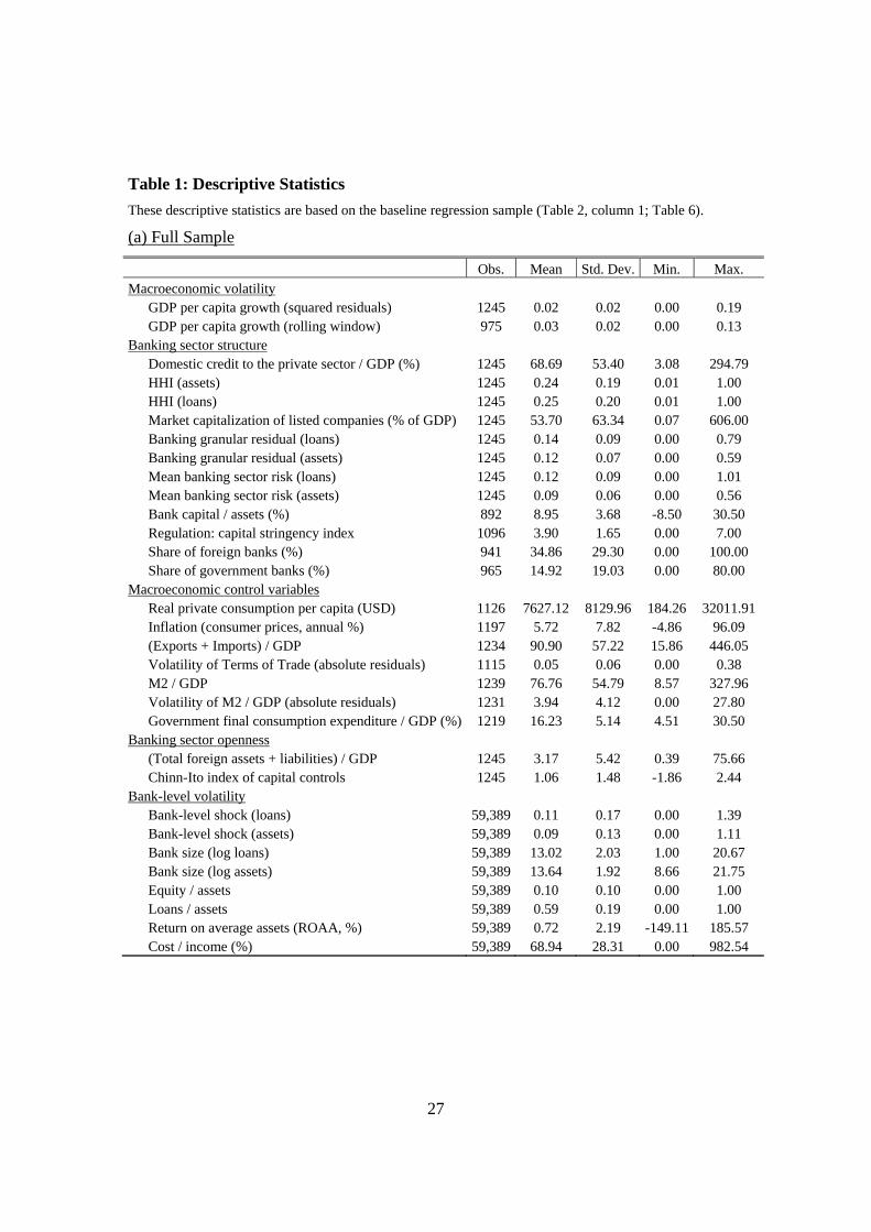
Table 1: Descriptive Statistics

These descriptive statistics are based on the baseline regression sample (Table 2, column 1; Table 6).

(a) Full Sample

Obs. Mean Std. Dev. Min. Max. Macroeconomic volatility

GDP per capita growth (squared residuals) 1245 0.02 0.02 0.00 0.19 GDP per capita growth (rolling window) 975 0.03 0.02 0.00 0.13

Banking sector structure Domestic credit to the private sector / GDP (%) 1245 68.69 53.40 3.08 294.79 HHI (assets) 1245 0.24 0.19 0.01 1.00 HHI (loans) 1245 0.25 0.20 0.01 1.00 Market capitalization of listed companies (% of GDP) 1245 53.70 63.34 0.07 606.00 Banking granular residual (loans) 1245 0.14 0.09 0.00 0.79 Banking granular residual (assets) 1245 0.12 0.07 0.00 0.59 Mean banking sector risk (loans) 1245 0.12 0.09 0.00 1.01 Mean banking sector risk (assets) 1245 0.09 0.06 0.00 0.56 Bank capital / assets (%) 892 8.95 3.68 -8.50 30.50 Regulation: capital stringency index 1096 3.90 1.65 0.00 7.00 Share of foreign banks (%) 941 34.86 29.30 0.00 100.00 Share of government banks (%) 965 14.92 19.03 0.00 80.00

Macroeconomic control variables Real private consumption per capita (USD) 1126 7627.12 8129.96 184.26 32011.91 Inflation (consumer prices, annual %) 1197 5.72 7.82 -4.86 96.09 (Exports + Imports) / GDP 1234 90.90 57.22 15.86 446.05 Volatility of Terms of Trade (absolute residuals) 1115 0.05 0.06 0.00 0.38 M2 / GDP 1239 76.76 54.79 8.57 327.96 Volatility of M2 / GDP (absolute residuals) 1231 3.94 4.12 0.00 27.80 Government final consumption expenditure / GDP (%) 1219 16.23 5.14 4.51 30.50

Banking sector openness (Total foreign assets + liabilities) / GDP 1245 3.17 5.42 0.39 75.66 Chinn-Ito index of capital controls 1245 1.06 1.48 -1.86 2.44

Bank-level volatility Bank-level shock (loans) 59,389 0.11 0.17 0.00 1.39 Bank-level shock (assets) 59,389 0.09 0.13 0.00 1.11 Bank size (log loans) 59,389 13.02 2.03 1.00 20.67 Bank size (log assets) 59,389 13.64 1.92 8.66 21.75 Equity / assets 59,389 0.10 0.10 0.00 1.00 Loans / assets 59,389 0.59 0.19 0.00 1.00 Return on average assets (ROAA, %) 59,389 0.72 2.19 -149.11 185.57 Cost / income (%) 59,389 68.94 28.31 0.00 982.54

28

(b) Low income countries

Obs. Mean Std. Dev. Min. Max. Macroeconomic volatility

GDP per capita growth (squared residuals) 174 0.02 0.02 0.00 0.11 GDP per capita growth (rolling window) 133 0.02 0.01 0.00 0.06

Banking sector structure Domestic credit to the private sector / GDP (%) 174 25.84 20.49 3.83 124.97 HHI (assets) 174 0.26 0.21 0.05 1.00 HHI (loans) 174 0.27 0.22 0.05 1.00Market capitalization of listed companies (% of GDP) 174 14.12 11.44 0.25 52.04 Banking granular residual (loans) 174 0.18 0.11 0.00 0.79 Banking granular residual (assets) 174 0.15 0.08 0.00 0.47 Mean banking sector risk (loans) 174 0.16 0.11 0.00 1.01 Mean banking sector risk (assets) 174 0.12 0.07 0.00 0.45 Bank capital / assets (%) 73 12.16 5.68 3.20 30.50 Regulation: capital stringency index 110 3.93 1.50 1.00 7.00 Share of foreign banks (%) 96 35.33 23.26 0.00 84.20 Share of government banks (%) 96 14.40 16.99 0.00 69.86

Macroeconomic control variables Real private consumption per capita (USD) 126 448.23 215.67 184.26 1108.32 Inflation (consumer prices, annual %) 174 9.07 6.13 -0.29 32.91 (Exports + Imports) / GDP 171 75.31 29.89 31.61 178.13 Volatility of Terms of Trade (absolute residuals) 170 0.07 0.07 0.00 0.33 M2 / GDP 174 37.63 21.09 10.38 125.11 Volatility of M2 / GDP (absolute residuals) 174 2.98 3.22 0.02 18.96 Government final consumption expenditure / GDP (%) 157 12.73 4.65 4.51 25.88

Banking sector openness (Total foreign assets + liabilities) / GDP 174 1.21 0.58 0.42 3.47 Chinn-Ito index of capital controls 174 0.13 1.37 -1.86 2.44

Bank-level volatility Bank-level shock (loans) 650 0.20 0.20 0.00 1.06 Bank-level shock (assets) 650 0.15 0.15 0.00 0.76 Bank size (log loans) 650 11.38 1.49 4.57 15.17 Bank size (log assets) 650 12.21 1.32 9.27 16.22 Equity / assets 650 0.16 0.12 0.01 0.81 Loans / assets 650 0.47 0.15 0.00 0.80 Return on average assets (ROAA, %) 650 2.09 2.92 -15.32 15.58 Cost / income (%) 650 65.56 41.68 8.49 600.00

29

Table 2: Determinants of the Volatility of GDP per Capita

The dependent variable is macroeconomic volatility measured as the absolute value of the residual of a regression of (log) growth in real GDP per capita on time and country fixed effects. Time and country fixed effects are included in all regressions but are not reported. ***, **, * = significant at the 1%, 5%, 10% level.

(1) (2) (3) (4) Banking Granular Residual BGR (assets) 0.013 0.022 (1.021) (1.380) Lagged BGR (assets, t-1) 0.007 0.003 (0.831) (0.308) Mean risk (assets) 0.012 0.013 (0.936) (0.919) Lagged mean risk (assets, t-1) 0.022** 0.011 (2.293) (1.029) HHI (assets) -0.004 -0.005 (-0.738) (-0.702) Banking market structure Domestic credit to private sector (% of GDP) 0.000** 0.000** 0.000*** 0.000*** (2.383) (2.460) (3.425) (3.286) (Foreign assets + liabilities) / GDP -0.000 -0.000* -0.000 -0.000 (-1.560) (-1.838) (-1.162) (-1.459) Chinn-Ito index of capital controls -0.003*** -0.003*** -0.005** -0.005** (-3.429) (-3.470) (-2.621) (-2.616) Market capitalization of listed companies (% of GDP) -0.000 -0.000 -0.000 -0.000 (-0.275) (-0.236) (-1.003) (-1.058) Macroeconomic control variables Private consumption per capita -0.000 -0.000 (-0.541) (-0.520) Government consumption expenditure (% of GDP) 0.001* 0.001* (1.834) (1.825) Inflation (consumer prices, annual %) 0.000* 0.000* (1.704) (1.710) Money and quasi money (M2) as % of GDP -0.000*** -0.000*** (-4.109) (-3.972) Absolute residual of M2 / GDP 0.000 0.000 (0.619) (0.557) (Imports + Exports) / GDP 0.000 0.000 (1.032) (1.000) Absolute residual of Terms of Trade -0.013 -0.012 (-0.611) (-0.546) Observations 1,245 1,245 972 972 R² 0.076 0.079 0.184 0.183 Number of countries 97 97 95 95

30

Table 3: Determinants of GDP Volatility by Income Group

The dependent variable is macroeconomic volatility measured as the absolute residual of a regression of growth in log real GDP per capita on time and country fixed effects. Time and country fixed effects are included in all regressions but are not reported. ***, **, * = significant at the 1%, 5%, 10% level.

(1) (2) (3) (4) (5) (6) Low income Middle income High income Banking Granular Residual BGR (assets) -0.048* 0.040 0.021 (-1.837) (1.234) (1.452) Lagged BGR (assets t-1) 0.049** -0.010 0.011 (2.437) (-0.580) (1.018) Mean risk (assets) -0.050* 0.028 0.014 (-1.888) (1.198) (0.869) Lagged mean risk (assets t-1) 0.057* -0.003 0.017 (1.825) (-0.141) (1.449) HHI (assets) -0.003 -0.005 -0.001 (-0.185) (-0.452) (-0.144) Banking market structure Domestic credit to private sector (% of GDP) 0.001** 0.001** 0.000* 0.000 0.000* 0.000* (2.295) (2.444) (1.772) (1.662) (1.716) (1.719) (Foreign assets + liabilities) / GDP 0.017*** 0.017** -0.000 -0.000 -0.000 -0.000 (3.223) (2.762) (-0.227) (-0.495) (-0.203) (-0.308) Chinn-Ito index of capital controls -0.012 -0.014 -0.002 -0.002 -0.008** -0.008** (-1.454) (-1.745) (-1.004) (-0.974) (-2.510) (-2.469) Market capitalization (% of GDP) 0.000 0.000 0.000 0.000 -0.000 -0.000 (0.100) (0.250) (0.324) (0.348) (-1.414) (-1.468) Macroeconomic control variables Private consumption per capita 0.000 0.000 -0.000* -0.000* 0.000 0.000 (1.609) (1.571) (-1.894) (-1.752) (0.471) (0.471) Government consumption expenditure (% of GDP) 0.002*** 0.002** 0.001** 0.001* 0.001 0.002 (3.543) (2.513) (2.122) (2.029) (0.782) (0.882) Inflation (consumer prices, annual %) -0.001 -0.001 0.000 0.000 -0.000 0.000 (-1.240) (-1.203) (1.614) (1.612) (-0.012) (0.019) Money and quasi money (M2) as % of GDP -0.001** -0.001** -0.000 -0.000 -0.000*** -0.000** (-2.684) (-2.551) (-1.451) (-1.442) (-2.777) (-2.597) Absolute residual of M2 / GDP -0.000 -0.000 0.000 0.000 0.000 -0.000 (-0.635) (-0.609) (0.554) (0.477) (0.004) (-0.004) (Imports + Exports) / GDP 0.000 0.000 0.000 0.000 0.000 0.000 (1.409) (1.288) (0.900) (0.948) (0.285) (0.260) Absolute residual of Terms of trade 0.043 0.042 0.014 0.016 -0.095** -0.094** (1.659) (1.614) (0.463) (0.511) (-2.620) (-2.618) Observations 126 126 433 433 413 413 R² 0.398 0.410 0.207 0.203 0.284 0.281 Number of countries 14 14 36 36 45 45

31

Table 4: Determinants of GDP-Volatility with Interaction Terms

The dependent variable is macroeconomic volatility measured as the absolute residual of a regression of growth in log real GDP per capita on time and country fixed effects. Time and country fixed effects are included in all regressions but are not reported. ***, **, * = significant at the 1%, 5%, 10% level.

(1) (2) (3) (4) Banking Granular Residual BGR (assets) 0.028* 0.029* (1.709) (1.718) BGR (assets) * Dummy(PRGT) -0.071*** -0.066** (-3.178) (-2.506) Lagged BGR (assets, t-1) -0.001 -0.000 (-0.063) (-0.035) Lagged BGR (assets) * Dummy(PRGT) 0.027 0.036 (0.905) (1.513) Mean risk (assets) 0.020 0.021 (1.329) (1.334) Mean risk (assets) * Dummy(PRGT) -0.055** -0.048 (-2.027) (-1.645) Lagged mean risk (assets, t-1) 0.007 0.007 (0.664) (0.668) Lagged mean risk (assets) * Dummy(PRGT) 0.034 0.045 (1.061) (1.560) HHI (assets) -0.007 -0.007 (-0.981) (-0.937) HHI (assets) * Dummy(PRGT) 0.020* 0.018 (1.721) (1.479) Banking market structure Domestic credit to private sector (% of GDP) 0.000*** 0.000*** 0.000*** 0.000*** (3.392) (3.278) (3.310) (3.178) Credit/GDP * Dummy(PRGT) -0.000 0.000 (-0.018) (0.360) (Foreign assets + liabilities) / GDP -0.000 -0.000 -0.000 -0.000 (-1.092) (-1.139) (-1.514) (-1.498) (Foreign assets + liabilities) / GDP * Dummy(PRGT) 0.006 0.006 (0.885) (0.916) Chinn-Ito index of capital controls -0.005*** -0.005** -0.005*** -0.005** (-2.666) (-2.541) (-2.638) (-2.515) Chinn-Ito index * Dummy(PRGT) -0.002 -0.004 (-0.439) (-0.713) Market capitalization (% of GDP) -0.000 -0.000 -0.000 -0.000 (-0.963) (-0.950) (-1.015) (-1.012) Macroeconomic control variables Private consumption per capita -0.000 -0.000 -0.000 -0.000 (-0.507) (-0.569) (-0.604) (-0.611) Government consumption expenditure (% of GDP) 0.001* 0.001* 0.001* 0.001* (1.809) (1.967) (1.871) (1.970) Inflation (consumer prices, annual %) 0.000* 0.000* 0.000* 0.000* (1.670) (1.661) (1.730) (1.701) Money and quasi money (M2) as % of GDP -0.000*** -0.000*** -0.000*** -0.000*** (-4.064) (-4.081) (-3.905) (-3.910) Absolute residual of M2 / GDP 0.000 0.000 0.000 0.000 (0.591) (0.634) (0.524) (0.543) (Imports + Exports) / GDP 0.000 0.000 0.000 0.000 (1.006) (1.044) (1.007) (1.012) Absolute residual of Terms of Trade -0.014 -0.015 -0.011 -0.012 (-0.634) (-0.662) (-0.519) (-0.553) Observations 972 972 972 972 R² 0.188 0.189 0.187 0.188 Number of countries 95 95 95 95

32

Table 5: Instrumental Variables Regressions

The dependent variable is macroeconomic volatility measured as the absolute residual of a regression of growth in log real GDP per capita on time and country fixed effects. Time and country fixed effects are included in all regressions but are not reported. ***, **, * = significant at the 1%, 5%, 10% level. (1) (2) Banking Granular Residual BGR (assets) -0.006 (-0.502) Lagged BGR (assets, t-1) 0.009 (0.823) Mean risk (assets) -0.003 (-0.285) Lagged mean risk (assets, t-1) 0.016 (1.236) HHI (assets) -0.003 (-0.207) Banking market structure Domestic credit to private sector (% of GDP) 0.001*** 0.000** (3.052) (2.308) (Foreign assets + liabilities) / GDP -0.000 -0.000 (-0.749) (-1.495) Chinn-Ito index of capital controls 0.004 0.001 (1.048) (0.136) Market capitalization (% of GDP) -0.000** -0.000* (-2.537) (-1.838) Macroeconomic control variables Private consumption per capita 0.000** 0.000** (2.357) (2.474) Government consumption expenditure (% of GDP) -0.002 -0.002 (-0.600) (-0.907) Inflation (consumer prices, annual %) 0.001* 0.000 (1.778) (0.167) Money and quasi money (M2) as % of GDP -0.001*** -0.000** (-4.090) (-2.610) Absolute residual of M2 / GDP -0.000 0.001 (-0.223) (0.906) (Imports + Exports) / GDP 0.000 0.000 (1.582) (0.533) Absolute residual of Terms of Trade -0.000 0.001 (-0.223) (0.906) Observations 689 689 R² 0.349 0.423 Number of countries 86 86 p-value of Hansen j-statistic 0.440 0.328 Hansen j-statistic 22.33 26.51

33

Table 6: Determinants of Idiosyncratic Bank-Level Volatility by Income Group The dependent variable is idiosyncratic asset volatility measured as the absolute value of the residual of a regression of growth in banks’ assets on country-time fixed effects. Country, bank and time fixed effects are included in all regressions but not reported. ***, **, * = significant at the 1%, 5%, 10% level.

(1) (2) (3) (4) (5) (6) (7) (8) Full sample Low Middle High Full sample Low Middle High Bank-level variables Log real assets -0.048* 0.114 -0.059*** -0.031 -0.045* 0.082 -0.060*** -0.027 (0.026) (0.339) (0.020) (0.033) (0.025) (0.343) (0.020) (0.032) Log real assets squared 0.002** -0.005 0.002*** 0.002 0.002** -0.003 0.002*** 0.002 (0.001) (0.012) (0.001) (0.001) (0.001) (0.012) (0.001) (0.001) Loans / assets -0.071*** -0.129*** -0.107*** -0.054** -0.073*** -0.106** -0.111*** -0.055** (0.020) (0.035) (0.034) (0.022) (0.020) (0.040) (0.036) (0.022) Bank equity to assets ratio (%) 0.001 0.007** 0.000 0.002 0.000 0.007** 0.000 0.001 (0.001) (0.003) (0.002) (0.002) (0.001) (0.002) (0.002) (0.002)Return on Average Assets (%) -0.002*** -0.003 -0.003*** -0.003*** -0.002*** -0.003 -0.003*** -0.003*** (0.000) (0.003) (0.001) (0.000) (0.000) (0.003) (0.001) (0.000) Cost to income ratio (%) 0.000*** 0.000 0.000 0.000*** 0.000*** 0.000 0.000 0.000*** (0.000) (0.000) (0.000) (0.000) (0.000) (0.000) (0.000) (0.000) Country-level variables Domestic credit to private sector (% of GDP) 0.000** -0.003 0.000 0.000 0.000** 0.003 0.000 0.000 (0.000) (0.003) (0.000) (0.000) (0.000) (0.003) (0.000) (0.000) HHI index assets for country j -0.032 -0.021 -0.182 -0.017 -0.030 0.102** -0.161 -0.014 (0.030) (0.033) (0.127) (0.026) (0.031) (0.037) (0.111) (0.027) (Foreign assets + liabilities) / GDP 0.000 0.093 -0.000 0.007*** 0.000 0.037 -0.000 0.007*** (0.001) (0.081) (0.000) (0.002) (0.001) (0.057) (0.000) (0.002) Chinn-Ito index of capital controls -0.010** -0.059 -0.004 -0.030*** -0.010** -0.100 -0.004 -0.027*** (0.005) (0.127) (0.003) (0.007) (0.004) (0.126) (0.004) (0.007) Capitalization (%) 0.111*** -0.033 0.076 0.138*** 0.114*** -0.012 0.073 0.142*** (0.028) (0.180) (0.053) (0.031) (0.029) (0.187) (0.054) (0.031) Capital stringency 0.001 -0.014 0.002 0.001 (0.001) (0.010) (0.002) (0.002) Share of foreign banks -0.000 -0.027*** -0.000 -0.000* (0.000) (0.003) (0.000) (0.000) Share of government banks -0.001* -0.006*** -0.000 -0.001** (0.000) (0.001) (0.000) (0.000) Observations 59,389 650 6,892 51,847 59,389 650 6,892 51,847 R² 0.023 0.158 0.030 0.027 0.024 0.174 0.031 0.028 Number of banks 8,869 137 1,187 7,545 8,869 137 1,187 7,545