banks non-interest income and systemic riskmarkus/research/papers/covar_non...banks’ non-interest...

Banks’ Non-Interest Income and Systemic Risk

Markus Brunnermeier,a Gang Dong,

b and Darius Palia

b

February, 2010

Abstract

This paper examines the contribution of non-interest income to systemic bank risk. Using

the ∆CoVaR measure of Adrian and Brunnermeier (2010) as our proxy for systemic risk, we

find banks with a higher non-interest income to interest income ratio have a higher contribution

to systemic risk. This suggests that activities that are not traditionally associated with banks

(such as deposit taking and lending) are associated with a larger contribution to systemic risk.

When we decompose total non-interest income into three components, we find trading income

and investment banking and venture capital income to be significantly related to systemic risk.

The economic impact on systemic risk of investment banking and venture capital income is

higher than that of trading income. Finally we find the impact of non-interest income on

systemic risk to be prevalent in the 1990 and 2007 financial crises (which were bank based) and

not in the case before the 2001 high tech bubble bust. These effects occur one-year before each

crisis and not during the recession, showing their countercyclical contribution to systemic risk

build-up.

aPrinceton University, NBER, CEPR, CESifo, and

bRutgers Business School, respectively. All errors remain our

responsibility.

1

“These banks have become trading operations. … It is the centre of their business.”

Phillip Angelides, Chairman, Financial Crisis Inquiry Commission

“The basic point is that there has been, and remains, a strong public interest in providing a “safety net”

– in particular, deposit insurance and the provision of liquidity in emergencies – for commercial banks

carrying out essential services (emphasis added). There is not, however, a similar rationale for public

funds – taxpayer funds – protecting and supporting essentially proprietary and speculative activities

(emphasis added)”

Paul Volcker, Statement before the US Senate’s Committee on Banking, Housing, & Urban Affairs

1. Introduction

The recent financial crisis of 2007-2009 has powerfully shown that risk spillovers from

one bank to another created significant systemic risk which was largely ignored by bankers,

investors and regulators. The infusion of taxpayer funds to commercial and investment banks

under the various programs of the government (Treasury and the Federal Reserve) have come

under increasing scrutiny (see for example the quotes above). But all banking activities are not

necessarily the same. One group of banking activities, namely, deposit taking and lending make

banks special to information-intensive borrowers and crucial for capital allocation in the

economy (for example, Bernanke 1983, Fama 1985, Diamond 1984, James 1987, Gorton and

Pennachi 1990, Calomiris and Kahn 1991, and Kashyap, Rajan, and Stein 2002). Such a view is

also articulated in the bank lending channel for the transmission of monetary policy (Bernanke

and Blinder 1988, Stein 1988, Kashyap, Stein and Wilcox 1993).

But banks have increasingly earned a higher proportion of their profits from non-interest

income when compared to interest income (see Table I). For example, the mean non-interest

income to interest income ratio has increased from 0.18 in 1989 to 0.59 in 2007 for the 10-

largest banks (by market capitalization in 2000, the middle of our sample). Non-interest income

includes activities such as income from trading and securitization, investment banking and

advisory fees, brokerage commissions, venture capital, and fiduciary income, and gains on non-

hedging derivatives. This paper examines the contribution of such non-interest income to

systemic bank risk. In these activities banks are competing with other capital market

intermediaries such as hedge funds, mutual funds, investment banks, insurance companies and

private equity funds, all of whom do not have federal deposit insurance. The existence of

insured deposits to commercial banks could lead to significant moral hazard resulting in higher

systemic risk.

2

*** Table I ***

In order to capture systemic risk in the banking sector we use the CoVaR measure of

Adrian and Brunnermier (2010; from now on referred to as AB).1 AB define CoVaR as the

Value at Risk (VaR) of the banking system, conditional on an individual bank being in distress.

More formally, it is the difference between the CoVaR conditional on a bank being in distress

and the CoVaR conditional on a bank operating in its median state (which AB refer to as

∆CoVaR). Such a measure is calculated one period forward and captures the marginal

contribution of a bank to overall systemic risk. AB suggests that prudential capital regulation

should not just be based on VaRs of a bank but also on their ∆CoVaRs, which by their predictive

power alert regulators (in our regressions by one-quarter ahead) who can use them as a basis for

a preemptive countercyclical capital regulation such as a capital surcharge or Pigovian tax.2

In this paper, we begin by estimating the ∆CoVaRs of all commercial banks (SIC codes

60 and 61) for the period 1986 to 2008. We examine three primary issues: (1) Is there a

relationship between systemic risk (or ∆CoVaR) and a bank’s non-interest income? (2) From

2001 onwards, banks were required to report detailed breakdowns of their non-interest income.

We categorize such items into three sub-groups, namely, trading income, investment banking

and venture capital income, and others. We examine if any sub-group has a significant effect on

systemic risk? (3) Finally, we examine if there were differential impacts of non-interest income

on systemic risk prior to and during the past three economic contractions (1990-91, 2000-01,

and 2007-08).

We find the following results:

1. We first find that systemic risk is higher for banks with a higher non-interest income to

interest income ratio. Specifically, a one standard deviation shock to a bank’s non-interest

income to interest income ratio increases its systemic risk contribution by 5.2%. This

suggests that activities that are not traditionally associated with banks (such as deposit taking

1 See Section 3 of this paper for more details.

2 AB calculates this measure for a portfolio of banks whereas we calculate it for individual banks. AB’s focus was

on showing that the CoVaR measure is valid as a measure of a bank’s contribution to systemic risk and therefore

can be used as a countercyclical capital charge measure. But our focus is on the marginal contribution of non-

interest income of individual banks on systemic risk. Given that a capital charge would be levied on an individual

bank, our paper also allows regulators to implement how the capital charge can be assessed.

3

and lending) are associated with a larger contribution to systemic risk. These results hold

when we use the systemic expected shortfall measure of Acharya, Pedersen, Philippon and

Richardson (2010).

2. We also find that larger banks (measured by asset size) and those with a higher ratio of

commercial & industrial loans to total loans contributed more to systemic risk. The result on

size is consistent with those found in AB and with the general idea that larger firms

contribute more to systemic risk.

3. When we can decompose total non-interest income into three components, we find trading

income and investment banking and venture income to be significantly related to systemic

risk. The economic impact on systemic risk of trading income is lower than that of

investment banking and venture capital income. A one standard deviation shock to a bank’s

trading income increases its systemic risk contribution by 2.9%, whereas a one standard

deviation shock to its investment banking and venture capital income increases its systemic

risk contribution by 5.4%.

4. During the previous three economic contractions, banks with a higher non-interest income to

interest income ratio contributed more to systemic risk in the 1990 and 2007 bank-based

crises; however this is not the case before the 2001 high tech bubble bust. Interestingly, these

results show up in end of the boom period (one-year before each crisis) and not during the

recession, showing their countercyclical contribution to systemic risk build-up.

In section 2 of this paper we describe the related literature and Section 3 explains our data

and methodology. Section 4 presents or empirical results and in Section 5 we conclude.

2. Related Literature

Recent papers have proposed complementary measures of systemic risk other than

∆CoVaR.3 We describe below some of the prominent measures. Acharya, Pedersen, Philippon

and Richardson (2010) propose the systemic expected shortfall (SES) which is the expected

amount a bank is undercapitalized in a systemic event in which the entire financial system is

undercapitalized. Allen, Bali and Tang (2010) propose the CATFIN measure which is the

3 See Billio, Getmansky Lo, and Pelizzon (2010) for a good survey.

4

principal components of the 1% VaR and expected shortfall, using estimates of the generalized

Pareto distribution, skewed generalized error distribution, and a non-parametric distribution.

Tarashev, Borio, and Tsatsaronis (2010) suggest Shapley values based on a bank’s of default

probabilities, size, and exposure to common risks could be used to assess regulatory taxes on

each bank. Chan-Lau (2010) proposes the CoRisk measure which captures the extent to which

the risk of one institution changes in response to changes in the risk of another institution while

controlling for common risk factors. Huang, Zhou, and Zhu (2009, 2010) propose the deposit

insurance premium (DIP) measure which is a bank’s expected loss conditional on the financial

system being in distress exceeding a threshold level.

Prior papers have also shown that non-interest income has generally increased the risk of

an individual bank but have not focused on a bank’s contribution to systemic risk. For example,

Stiroh (2004) and Fraser, Madura, and Weigand (2002) finds that non-interest income is

associated with more volatile bank returns. DeYoung and Roland (2001) find fee-based

activities are associated with increased revenue and earnings variability. Stiroh (2006) finds that

non-interest income has a larger effect on individual bank risk in the post-2000 period. In a

study of Italian banks, Acharya, Hassan and Saunders (2006) find diseconomies of scope when

a risky bank expands into additional sectors.

A number of papers have used the CoVaR measure in other contexts. Wong and Fong

(2010) examine ∆CoVaR for credit default swaps of Asia-Pacific banks, whereas Gauthier,

Lehar and Souissi (2010) use it for Canadian institutions. Adams, Fuss and Gropp (2010) study

risk spillovers among financial institutions including hedge funds, and Zhou (2009) uses

extreme value theory rather than quantile regressions to get a measure of CoVaR.

3. Data, Methodology, and Variables Used

We focus on all publicly traded bank holding companies in the U.S., namely, with SIC

codes 60 or 61 (for commercial banks) and using the Fama-French SIC code classification for

banks, namely, “portfolio 44.” By focusing on commercial banks we do not include insurance

companies, investment banks, investment management companies, and brokers. Our sample is

from 1986 to 2008, and consists of an unbalanced panel of 538 unique banks. Four of these

banks have zero non-interest income. We obtain a bank’s daily equity returns from CRSP which

5

we use to convert into weekly returns. Financial statement data is from Compustat and from

Federal Reserve form FR Y-9C filed by a bank with the Federal Reserve. T-bill and LIBOR

rates are from the Federal Reserve Bank of New York and real estate market returns are from

the Federal Housing Finance Agency. The dates of recessions are obtained from the NBER

(http://www.nber.org/cycles/cyclesmain.html). Detailed sources for each specific variable used

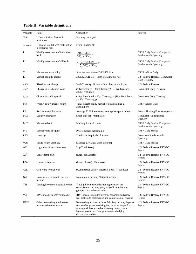
in our estimation are given in Table II.

*** Table II ***

We describe below how we calculate the ∆CoVaR measure of Adrian and Brunnermeier

(2010).

Value-at-Risk (VaR)4 measures the worst expected loss under normal market conditions

over a specific time interval at a given confidence level. In the context of this paper, i

qVaR is

defined as the percentage iR of asset value that bank i might lose with %q probability over a

pre-set horizon T :

( )i i

qProbability R VaR q (1)

Thus by definition the value of VaR is negative in general.5 Another way of expressing this is

that i

qVaR is the %q quantile of the potential asset return in percentage term ( iR ) that can occur

to bank i during a specified time period T. The confidence level (quantile) q and the time period

T are the two major parameters in a traditional risk measure using VaR. We consider 1%

quantile and weekly asset return/loss iR in this paper, and the VaR of bank i is

1%( ) 1%i iProbability R VaR .

Let |system i

qCoVaR denote the Value at Risk of the entire financial system conditional upon

bank i being in distress (in other words, the loss of bank i is at its level of i

qVaR ). That is,

4 See Philippe (2006, 2009) for detail definition, discussion and application of VaR.

5 Empirically the value of VaR can also be positive. For example, VaR is used to measure the investment risk in a

AAA coupon bond. Assume that the bond was sold at discount and the market interest rate is continuously falling,

but never below the coupon rate during the life the investment. Then the q% quantile of the potential bond return is

positive, because the bond price increases when the market interest rate is falling.

http://www.nber.org/cycles/cyclesmain.html

6

|system i

qCoVaR which essentially is a measure of systemic risk is the q% quantile of this

conditional probability distribution:

|( | )system system i i i

q qProbability R CoVaR R VaR q (2)

Similarly, let | ,system i median

qCoVaR denote the financial system’s VaR conditional on bank i

operating in its median state (in other words, the return of bank i is at its median level). That is,

| ,system i median

qCoVaR measures the systemic risk when business is normal for bank i :

| ,( | )system system i median i i

qProbability R CoVaR R median q (3)

Bank i ’s contribution to systemic risk can be defined as the difference between the

financial system’s VaR conditional on bank i in distress ( |system i

qCoVaR ), and the financial

system’s VaR conditional on bank i functioning in its median state ( | ,system i median

qCoVaR ):

| | ,i system i system i median

q q qCoVaR CoVaR CoVaR (4)

In the above equation, the first term on the right hand side measures the systemic risk when

bank i ’s return is in its q% quantile (distress state), and the second term measures the systemic

risk when bank i ’s return is at its median level (normal state).

To estimate this measure of individual bank’s systemic risk contribution i

qCoVaR , we

need to calculate two conditional VaRs for each bank, namely |system i

qCoVaR and

| ,system i median

qCoVaR . For the systemic risk conditional on bank i in distress ( |system i

qCoVaR ), run a

1% quantile regression6 using the weekly data to estimate the coefficients i , i , |system i ,

|system i and |system i :

6 See Appendix A for detail explanation of our quantile regressions.

7

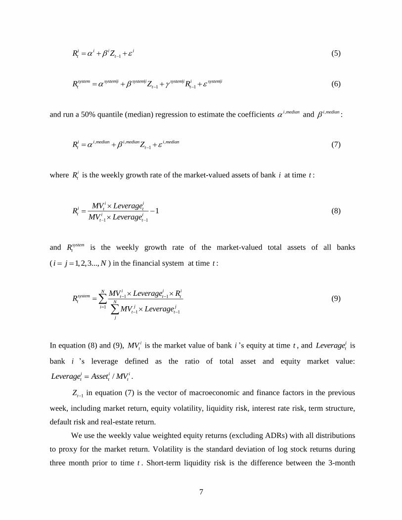
1

i i i i

t tR Z (5)

| | | |

1 1

system system i system i system i i system i

t t tR Z R (6)

and run a 50% quantile (median) regression to estimate the coefficients ,i median and ,i median :

, , ,

1

i i median i median i median

t tR Z (7)

where i

tR is the weekly growth rate of the market-valued assets of bank i at time t :

1 1

1i i

i t tt i i

t t

MV LeverageR

MV Leverage

(8)

and system

tR is the weekly growth rate of the market-valued total assets of all banks

( 1,2,3...,i j N ) in the financial system at time t :

1 1

11 1

i i iNsystem t t tt N

j jit t

j

MV Leverage RR

MV Leverage

(9)

In equation (8) and (9), i

tMV is the market value of bank i ’s equity at time t , and i

tLeverage is

bank i ’s leverage defined as the ratio of total asset and equity market value:

/i i i

t t tLeverage Asset MV .

1tZ in equation (7) is the vector of macroeconomic and finance factors in the previous

week, including market return, equity volatility, liquidity risk, interest rate risk, term structure,

default risk and real-estate return.

We use the weekly value weighted equity returns (excluding ADRs) with all distributions

to proxy for the market return. Volatility is the standard deviation of log stock returns during

three month prior to time t . Short-term liquidity risk is the difference between the 3-month

8

LIBOR rate and the 3-month T-bill rate. Interest rate risk is the change in the 3-month T-bill

rate. We use the change in the slope of the yield curve (yield spread between the 10-year T-bond

rate and the 3-month T-bill rate) to proxy for the term structure. Default risk is the change in the

credit spread between the 10-year BAA corporate bonds and the 10-year T-bond rate. Real

estate return is based on the FHFA house price index. See Table II for details of our data

sources.

*** Table II ***

Hence we predict an individual bank’s VaR and median asset return using the coefficients

ˆ i , ˆ i , ,ˆ i median and ,ˆ i median estimated from the quantile regressions of equation (5) and (7):

, 1ˆˆ ˆi i i i

q t t tVaR R Z (10)

, , ,

1ˆˆ ˆi median i i median i median

t t tR R Z (11)

The vector of state (macroeconomic and finance) variables 1tZ is the same as in equation (5)

and (7). After obtaining the unconditional VaRs of an individual bank i ( ,

i

q tVaR ) and that bank’s

asset return in its median state ( ,i median

tR ) from equation (10) and (11), we predict the systemic

risk conditional on bank i in distress ( |system i

qCoVaR ) using the coefficients |ˆ system i , |ˆ system i ,

|ˆsystem i estimated from the quantile regression of equation (6) . Specifically,

| | | |

, 1 ,ˆˆ ˆ ˆsystem i system system i system i system i i

q t t t q tCoVaR R Z VaR (12)

Similarly, we can calculate the systemic risk conditional on bank i functioning in its median

state (| ,system i median

qCoVaR ) as :

| , | | | ,

, 1ˆˆ ˆsystem i median system i system i system i i median

q t t tCoVaR Z R (13)

9

Bank i ’s contribution to systemic risk is the difference between the financial system’s VaR if

bank i is at risk and the financial system’s VaR if bank i is in its median state:

| | ,

, , ,

i system i system i median

q t q t q tCoVaR CoVaR CoVaR (14)

Note that this is same as equation (4) with an additional subscript t to denote the time-varying

nature of the systemic risk in the banking system. As shown in the quantile regressions of

equation (5) and (7), we are interested in the VaR at the 1% confident level, therefore the

systemic risk of individual bank at q=1% can be written as:

| | ,

1%, 1%, 1%,


t t tCoVaR CoVaR CoVaR (15)

To investigate the relationship between the bank characteristics and lagged bank’s

contribution to systemic risk, we run OLS regressions with quarterly fixed effects and the

following bank-specific variables: maturity mismatch (MM), market to book (M2B), financial

leverage (LEV), total asset (AT), loan to asset (L2A), C&I loan to total loan (C2A), and non-

interest income to interest income (N2I).

2

t 0 1 t 1 2 t 1 3 t 1 4 t 1 5 t 1 6 t 1 7 t 1CoVaR VaR MM M 2B LEV VOL AT AT

( )8 t 1 9 t 1 10 t 1 tL2A CI2L N2I FE quarterly (16)

We focus on the impact of bank’s N2I ratio (non-interest income to interest income ratio) on its

systemic risk contribution.

From 2001 onwards, we can decompose this N2I ratio into its three components, namely,

trading income to interest income (T2I), investment banking and venture income to interest

income (V2I), and other non-interest income to non-interest income (NT2I). We regress the

individual bank’s systemic risk contribution (∆CoVaR) on its T2I, V2I and NT2I ratios along

with other control variables and include quarterly fixed effects.

10

2

t 0 1 t 1 2 t 1 3 t 1 4 t 1 5 t 1 6 t 1 7 t 1CoVaR VaR MM M 2B LEV VOL AT AT

( )8 t 1 9 t 1 10 t 1 11 t 1 12 t 1 tL2A CI2L T2I V 2I NT2I FE quarterly

(17)

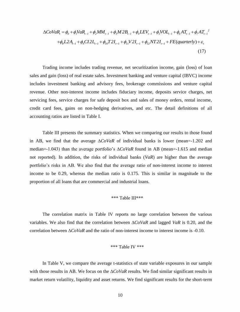
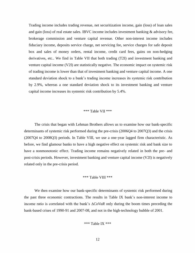
Trading income includes trading revenue, net securitization income, gain (loss) of loan

sales and gain (loss) of real estate sales. Investment banking and venture capital (IBVC) income

includes investment banking and advisory fees, brokerage commissions and venture capital

revenue. Other non-interest income includes fiduciary income, deposits service charges, net

servicing fees, service charges for safe deposit box and sales of money orders, rental income,

credit card fees, gains on non-hedging derivatives, and etc. The detail definitions of all

accounting ratios are listed in Table I.

Table III presents the summary statistics. When we comparing our results to those found

in AB, we find that the average ∆CoVaR of individual banks is lower (mean=-1.202 and

median=-1.043) than the average portfolio’s ∆CoVaR found in AB (mean=-1.615 and median

not reported). In addition, the risks of individual banks (VaR) are higher than the average

portfolio’s risks in AB. We also find that the average ratio of non-interest income to interest

income to be 0.29, whereas the median ratio is 0.175. This is similar in magnitude to the

proportion of all loans that are commercial and industrial loans.

*** Table III***

The correlation matrix in Table IV reports no large correlation between the various

variables. We also find that the correlation between ∆CoVaR and lagged VaR is 0.20, and the

correlation between ∆CoVaR and the ratio of non-interest income to interest income is -0.10.

*** Table IV ***

In Table V, we compare the average t-statistics of state variable exposures in our sample

with those results in AB. We focus on the ∆CoVaR results. We find similar significant results in

market return volatility, liquidity and asset returns. We find significant results for the short-term

11

rate change, term structure, default credit spread, and changes in house prices, whereas AB finds

statistically insignificant results on these factors. AB find market returns to be statistically

significant whereas we find it to be insignificant.

*** Table V ***

4. Empirical Results

We begin by examining the Table VI. The dependent variable is ∆CoVaR. All independent

variables are estimated with a one quarter lag, and we also include quarter fixed-effects which

are not reported. The t-statistics are calculated using Newey-West standard errors which

rectifies for heteroskedasticity. The independent variables are individual bank’s maturity

mismatch (MM), market to book ratio (M2B), financial leverage ratio (LEV), total assets (AT),

loan to asset ratio (L2A), the ratio of commercial and industrial loans to total loans (C2L), and

non-interest income to interest income (N2I). Given that ∆CoVaR is defined as systemic risk

contribution when the bank is in distress compared to its contribution when the bank operates in

its median state, a negative (positive) coefficient implies higher (lower) systemic risk next

quarter. We find that glamour banks, and banks with a higher proportion of their loans in

commercial and industrial loans contribute more to systemic risk. The effect of bank size is

nonmonotonic, whereas a higher proportion of loans to assets help reduce systemic risk.

Importantly, we find that the ratio of non-interest income to interest income is significantly

negative suggesting that it contributes adversely to systemic risk. Specifically, a one standard

deviation shock to a bank’s non-interest income to interest income ratio increases its systemic

risk contribution by 5.2%.

*** Table VI ***

From 2001 onwards, we can decompose the ratio of non-interest income to interest

income into trading income to interest income (T2I), investment banking and venture capital

income to interest income (V2I), and other non-interest income to interest income (NT2I),

respectively. Federal Reserve form FR Y-9C only gives these detailed data after 2001.

12

Trading income includes trading revenue, net securitization income, gain (loss) of loan sales

and gain (loss) of real estate sales. IBVC income includes investment banking & advisory fee,

brokerage commission and venture capital revenue. Other non-interest income includes

fiduciary income, deposits service charge, net servicing fee, service charges for safe deposit

box and sales of money orders, rental income, credit card fees, gains on non-hedging

derivatives, etc.. We find in Table VII that both trading (T2I) and investment banking and

venture capital income (V2I) are statistically negative. The economic impact on systemic risk

of trading income is lower than that of investment banking and venture capital income. A one

standard deviation shock to a bank’s trading income increases its systemic risk contribution

by 2.9%, whereas a one standard deviation shock to its investment banking and venture

capital income increases its systemic risk contribution by 5.4%.

*** Table VII ***

The crisis that began with Lehman Brothers allows us to examine how our bank-specific

determinants of systemic risk performed during the pre-crisis (2006Q4 to 2007Q3) and the crisis

(2007Q4 to 2008Q3) periods. In Table VIII, we use a one-year lagged firm characteristic. As

before, we find glamour banks to have a high negative effect on systemic risk and bank size to

have a nonmonotonic effect. Trading income remains negatively related in both the pre- and

post-crisis periods. However, investment banking and venture capital income (V2I) is negatively

related only in the pre-crisis period.

*** Table VIII ***

We then examine how our bank-specific determinants of systemic risk performed during

the past three economic contractions. The results in Table IX bank’s non-interest income to

income ratio is correlated with the bank’s ∆CoVaR only during the boom times preceding the

bank-based crises of 1990-91 and 2007-08, and not in the high-technology bubble of 2001.

*** Table IX ***

13

We now examine if our results are driven by characteristics of ∆CoVaR that might not

capture real systemic risk. We use the systemic expected shortfall (SES) measure of Acharya,

Pedersen, Philippon and Richardson (2010) as our definition of systemic risk. In Appendix B we

explain how we calculate SES using cross-sectional quarterly data. The results of such a

regression are given in Table X. Once again we find that the ratio of non-interest income to

interest income is significantly negative suggesting that it contributes adversely to systemic risk.

Specifically, a one standard deviation shock to a bank’s non-interest income to interest income

ratio increases the mean SES measure of -6.98% by -2.47%, an increase of 35%. This suggests

that the relationship between non-interest income and systemic risk does not depend on our

proxy for systemic risk.

*** Table X ***

Robustness Tests: We run a number of robustness tests. First, we address the concern

that the bank’s non-interest income to income ratio is also correlated with the bank’s VaR. In

columns (1) and (2) of Table XI we find no evidence of this. Second, in columns (3)-(5) of

Table XI we find different lags of the bank’s non-interest income to income ratio is correlated

with the bank’s ∆CoVaR. This suggests our results are robust to various lagged quarters.

*** Table XI ***

Third, we examine if our result is driven by the numerator (non-interest income) and not

the denominator (net interest income). In Table XII, we reestimate our regressions using the

ratio of non-interest income to assets instead of non-interest income to interest. We find that

non-interest income is once again negatively related suggesting that it contributes adversely to

systemic risk.7 Similar relationships are found for trading income and for investment banking

and venture capital income. These results suggest that it is non-traditional income (namely, non-

7 We also reestimated the SES measure of systemic risk while including the ratio of non-interest income to assets.

We find similar results (results not reported but available from the authors).

14

interest income) that contributes adversely to systemic risk, and not traditional income (namely,

interest income).

*** Table XII ***

Fourth, we examine if changes in the state variables (Zt) are the primary force driving our

results. To do so, we use as our dependent variable, the bank’s ∆CoVaR in the same quarter

instead of one-quarter ahead. In Table XIII we find that banks’ with a higher non-interest

income to income ratio is correlated with ∆CoVaR in the same quarter. We also find that

investment banking, venture capital and trading income contributed more to systemic risk.

These results are consistent with those found before, and suggest that changes in the state

variables are not driving our results.

*** Table XIII ***

Fifth, we examine if our results can be explained by fair-value accounting issues. Given

that non-interest income consists generally of items which are marked to market, and interest

income includes items such as interest on loans and deposits which are at historical cost, we

examine if our results are driven by fair-value accounting issues. In order do so, we split

investment banking and venture capital to interest income ratio (V2I) into two ratios: investment

banking to interest income ratio, and venture capital to interest income ratio, respectively.

Investment banking consists of advisory fees and underwriting commissions which are not

marked to market, whereas venture capital includes revenues from holdings in companies in

which banks have taken to market and which are generally marked to market. If our results are

driven by marked to market issues, the regression coefficient of venture capital should be

negative and larger (in absolute terms) than the regression coefficient of investment banking. In

fact, we find the opposite (results not reported but available from the authors). We find the

regression coefficient of venture capital to be positive but not statistically significant and the

regression coefficient of investment banking to be positive. These results suggest that mark to

market accounting does not explain the contribution of non-interest income to systemic risk, and

is generally consistent with the results in Laux and Leunz (2010) and studies cited therein.

15

Sixth, we address the concern that our results are driven by volatile non-interest income

(i.e., in time-series) or by cross-sectional bank characteristics. We break down the ratio of non-

interest to interest income (N2I) ratio into three terciles, and count the numbers of banks shifting

between terciles. Table XIV provides the number of banks whose N2I ratios changed between

different terciles in each calendar quarter. Both the mean and median percentage of banks

drifting from one tercile to another during a quarter are only 4% of the total number of the banks,

implying that it is indeed the cross-sectional bank characteristics driving our results and not the

time-series effect.

*** Table XIV ***

5. Conclusions

The recent financial crisis showed that negative externalities from one bank to another

created significant systemic risk. This resulted in significant infusions of funds from the Federal

Reserve and the Treasury given that deposit taking and lending make banks special to

information-intensive borrowers and for the bank lending channel transmission mechanism of

monetary policy. But banks have increasingly earned a higher proportion of their profits from

non-interest income from activities such as trading, investment banking, venture capital and

advisory fees. This paper examines the contribution of such non-interest income to systemic

bank risk.

Using the ∆CoVaR measure of Adrian and Brunnermeier (2010) as our proxy for

systemic risk, we find banks with a higher non-interest income to interest income ratio have a

higher contribution to systemic risk. This suggests that activities that are not traditionally

associated with banks (such as deposit taking and lending) are associated with a larger systemic

risk. We also find that larger banks (measured by asset size) and those with a higher ratio of

commercial and industrial loans to total loans contributed more to systemic risk. When we

decompose the total non-interest income into three components, we find trading income and

investment banking and venture capital income to be significantly related to systemic risk. The

economic impact on systemic risk of trading income is lower than that of investment banking

16

and venture capital income. Finally we find the impact of non-interest income on systemic risk to

be prevalent in 1990 and 2007 financial crises (which were bank based) and not in the case

before the 2001 high tech bubble bust. Interestingly, these results show up in end of the boom

period (one-year before each crisis) and not during the recession, showing their countercyclical

contribution to systemic risk build-up.

17

Appendix A: Quantile Regression

OLS regression models the relationship between the independent variable X and the

conditional mean of a dependent variable Y given X = X1, X2, … Xn, as shown in Figure 1. In

contrast, quantile regression8 models the relationship between X and the conditional quantiles of

Y given X = X1, X2, … Xn, thus it provides a more complete picture of the conditional distribution

of Y given X when the lower or upper quantile is of interest. It is especially useful in

applications of Value at Risk (VaR), where the lowest 1% quantile is an important measure of

risk.

*** Figure 1 ***

Consider the quantile regression in equation (5): 1

i i i i

t tR Z , the dependent

variable Y is bank i ’s weekly asset return ( i

tR ) and the independent variable X is the exogenous

state (macroeconomic and finance) variables ( 1tZ ) of the previous period. The predicted value

( ˆ i

tR ) using the coefficient estimates ( ˆ i and ˆ i ) from the 1%-quantile regression and the

lagged state variable ( 1tZ ) is bank i ’s VaR at 1% confident level in that week:

1%, 1ˆˆ ˆi i i i

t t tVaR R Z . Similarly the predicted value ( ˆ system

tR ) in equation (12) using the

coefficient estimates ( |ˆ system i , |ˆ system i and |ˆsystem i ) from equation (6), the lagged state variable

( 1tZ ), and the 1%,

i

tVaR calculated above is the financial system’s VaR (|

,

system i

q tCoVaR )

conditional on bank i ’s return being at its lowest 1% quantile ( i

tVaR ):

| | | |

1%, 1 1%,ˆˆ ˆ ˆsystem i system system i system i system i i

t t t tCoVaR R Z VaR .

Note that the 50% quantile regression is also called median regression. Like the

conditional mean regression (OLS), the conditional median regression can represent the

relationship between the central location of the dependent variable Y and the independent

variable X. However, when the distribution of Y is skewed as shown in Figure 1, the mean can be

8 Koenker and Hallock (2001) provide a general introduction of quantile regression. Bassett and Koenker (1978) and

Koenker and Bassett (1978) discuss the finite sample and asymptotic properties of quantile regression. Koenker

(2005) is a comprehensive reference of the subject with applications in economics and finance.

18

challenging to interpret while the median remains highly informative.9 As a consequence, it is

appropriate in our study to use median regression to estimate the financial system’s risk

( | ,

1%

system i medianCoVaR ) when an individual bank is operating in its median state. The predicted value

( ˆ i

tR ) using the coefficient estimates ( ,ˆ i median and ,ˆ i median ) from the 1%-quantile regression in

equation (7) and the lagged state variable ( 1tZ ) is bank i ’s median return:

, , ,

1ˆˆi median i median i median

t tR Z .

Following the same method, the financial system’s risk conditional on bank i operating in

its median state ( | ,

1%

system i medianCoVaR ) is calculated using the coefficient estimates |ˆ system i , |ˆ system i ,

|ˆsystem i from equation (6), the state variable ( 1tZ ), and the median return of bank i ( ,i median

tR ):

| , | | | ,

, 1ˆˆ ˆsystem i median system i system i system i i median

q t t tCoVaR Z R .

Finally, the measure of bank i ’s contribution of systemic risk (CoVaR) is the difference

between |

,

system i

q tCoVaR and | ,

1%

system i medianCoVaR : | | ,

1%, 1%, 1%,


t t tCoVaR CoVaR CoVaR . It is

obvious that the calculation can be simplified to: | ,

1%, 1%,( )i system i i i median

t t tCoVaR VaR R as

shown in Adrian and Brunnermeier (2010).

9 The asymmetric properties of stock return distributions have been studied in Fama (1965), Officer (1972), and

Praetz (1972).

19

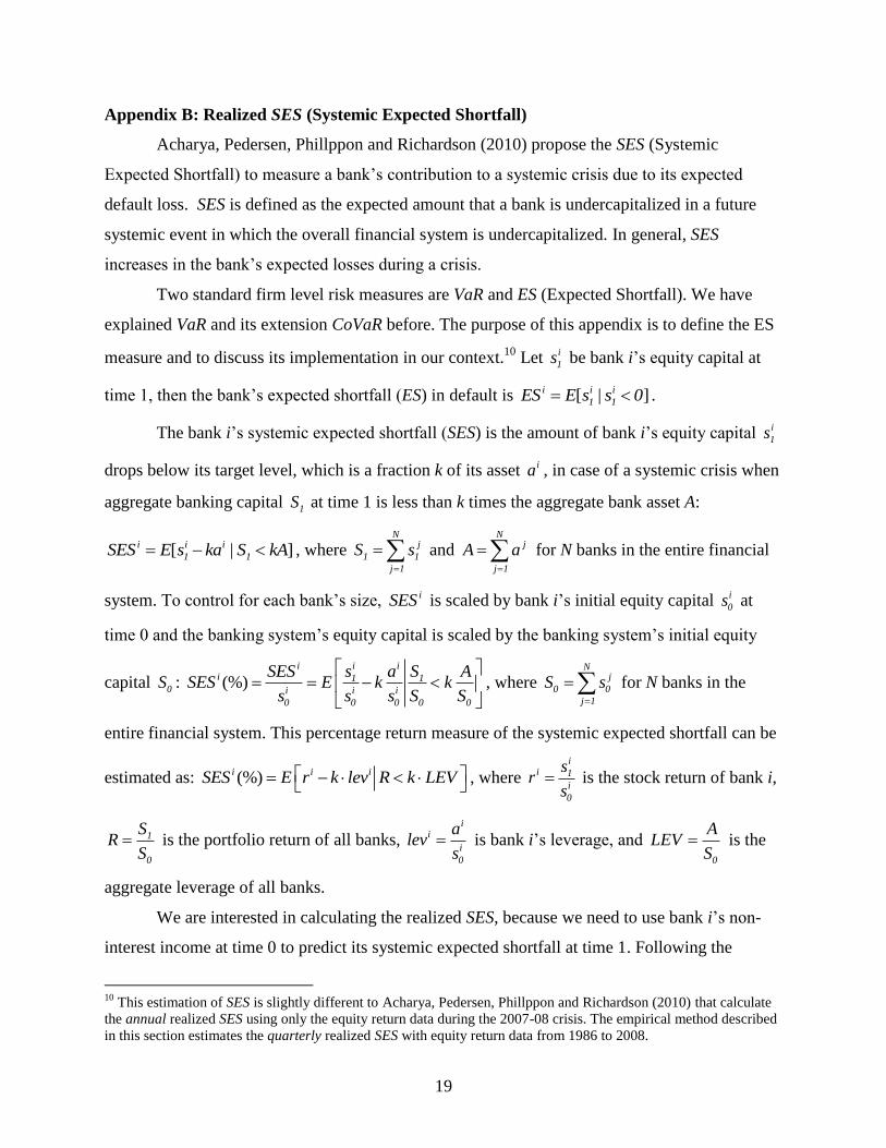
Appendix B: Realized SES (Systemic Expected Shortfall)

Acharya, Pedersen, Phillppon and Richardson (2010) propose the SES (Systemic

Expected Shortfall) to measure a bank’s contribution to a systemic crisis due to its expected

default loss. SES is defined as the expected amount that a bank is undercapitalized in a future

systemic event in which the overall financial system is undercapitalized. In general, SES

increases in the bank’s expected losses during a crisis.

Two standard firm level risk measures are VaR and ES (Expected Shortfall). We have

explained VaR and its extension CoVaR before. The purpose of this appendix is to define the ES

measure and to discuss its implementation in our context.10

Let i

1s be bank i’s equity capital at

time 1, then the bank’s expected shortfall (ES) in default is [ | ]i i i

1 1ES E s s 0 .

The bank i’s systemic expected shortfall (SES) is the amount of bank i’s equity capital i

1s

drops below its target level, which is a fraction k of its asset ia , in case of a systemic crisis when

aggregate banking capital 1S at time 1 is less than k times the aggregate bank asset A:

[ | ]i i i

1 1SES E s ka S kA , where N

j

1 1

j 1

S s

and N

j

j 1

A a

for N banks in the entire financial

system. To control for each bank’s size, iSES is scaled by bank i’s initial equity capital i

0s at

time 0 and the banking system’s equity capital is scaled by the banking system’s initial equity

capital 0S : (%)ii i

i 1 1

i i i

0 0 0 0 0

s SSES a ASES E k k

s s s S S

, where

Nj

0 0

j 1

S s

for N banks in the

entire financial system. This percentage return measure of the systemic expected shortfall can be

estimated as: (%)i i iSES E r k lev R k LEV

, where i

i 1

i

0

sr

s is the stock return of bank i,

1

0

SR

S is the portfolio return of all banks,

ii

i

0

alev

s is bank i’s leverage, and

0

ALEV

S is the

aggregate leverage of all banks.

We are interested in calculating the realized SES, because we need to use bank i’s non-

interest income at time 0 to predict its systemic expected shortfall at time 1. Following the

10

This estimation of SES is slightly different to Acharya, Pedersen, Phillppon and Richardson (2010) that calculate

the annual realized SES using only the equity return data during the 2007-08 crisis. The empirical method described

in this section estimates the quarterly realized SES with equity return data from 1986 to 2008.

20

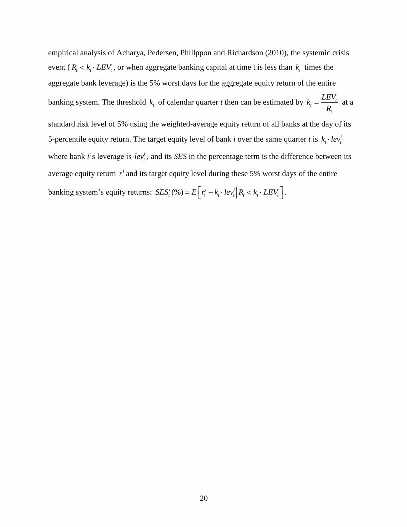
empirical analysis of Acharya, Pedersen, Phillppon and Richardson (2010), the systemic crisis

event ( t t tR k LEV , or when aggregate banking capital at time t is less than tk times the

aggregate bank leverage) is the 5% worst days for the aggregate equity return of the entire

banking system. The threshold tk of calendar quarter t then can be estimated by tt

t

LEVk

R at a

standard risk level of 5% using the weighted-average equity return of all banks at the day of its

5-percentile equity return. The target equity level of bank i over the same quarter t is i

t tk lev

where bank i’s leverage is i

tlev , and its SES in the percentage term is the difference between its

average equity return i

tr and its target equity level during these 5% worst days of the entire

banking system’s equity returns: (%)i i i

t t t t t t tSES E r k lev R k LEV

.

21

References

Acharya, Viral, Iftekhar Hasan, and Anthony Saunders, 2006, “Should Banks Be Diversified?

Evidence from Individual Bank Loan Portfolios,” Journal of Business 79, 1355-1412.

Acharya, Viral, Lasse Pedersen, Thomas Philippon, and Mathew Richardson, 2010, “Measuring

Systemic Risk,” NYU Stern Working Paper.

Acharya, Viral, and Matthew Richardson, 2009, Restoring Financial Stability, John Wiley &

Sons Inc.

Allen, Linda, Turan Bali, and Yi Tang, 2010, “Does Systemic Risk in the Financial Sector

Predict Future Economic Downturns?,” Baruch College Working Paper.

Adams, Zeno, Roland Fuss, and Reint Gropp, 2010, “Modeling Spillover Effects among

Financial Institutions: A State-Dependent Sensitivity Value-at-Risk (SDSVaR) Approach,” EBS

Working Paper.

Adrian, Tobias, and Markus Brunnermeier, 2010, “CoVaR,” Fed Reserve Bank of New York

Staff Reports.

Bassett, Gilbert and Roger Koenker, 1978, “Asymptotic Theory of Least Absolute Error

Regression,” Journal of the American Statistical Association 73, 618-622.

Bernanke, Ben, 1983, “Nonmonetary Effects of the Financial Crisis in the Propagation of the

Great Depression,” American Economic Review 73, 257-276.

Bernanke, Ben, and Alan Blinder, 1988, “Credit, Money, and Aggregate Demand,” American

Economic Review 78, 435-439.

Calomiris, Charles, and Charles Kahn, 1991, “The Role of Demandable Debt in Structuring

Optimal Banking Arrangements,” American Economic Review 81, 497-513.

Chan-Lau, Jorge, 2010, “Regulatory Capital Charges for Too-Connected-to-Fail Institutions: A

Practical Proposal,” IMF Working Paper 10/98.

DeYoung, Robert, and Karin Roland, 2001, “Product Mix and Earnings Volatility at Commercial

Banks: Evidence from a Degree of Total Leverage Model,” Journal of Financial Intermediation

10, 54-84.

Diamond, Douglas, 1984, “Financial Intermediation and Delegated Monitoring,” Review of

Economic Studies 51, 393-414.

Fama, Eugene, 1965, “The Behavior of Stock Market Prices,” Journal of Business 37, 34-105.

Fama, Eugene, 1985, “What's Different About Banks?,” Journal of Monetary Economics 15, 29-

39.

22

Fraser, Donald, Jeff Madura, and Robert Weigand, 2002, “Sources of Bank Interest Rate Risk,”

Financial Review 37, 351-367.

Gauthier, Celine, Alfred Lehar, and Moez Souissi, 2010, “Macroprudential Capital Requirements

and Systemic Risk,” Bank of Canada Working Paper 2010-4.

Gorton, Gary, and George Pennacchi, 1990, “Financial Intermediaries and Liquidity Creation,”

Journal of Finance 45, 49-71.

Huang, Xin, Hao Zhou, and Haibin Zhu, 2009, “A Framework for Assessing the Systemic Risk

of Major Financial Institutions,” Journal of Banking and Finance 33, 2036-2049.

Huang, Xin, Hao Zhou, and Haibin Zhu, 2010, “Systemic Risk Contributions,” FRB Working

Paper.

James, Christopher, 1987, “Some Evidence on the Uniqueness of Bank Loans,” Journal of

Financial Economics 19, 217-235.

Jorion, Philippe, 2006, Value at Risk: The New Benchmark for Managing Financial Risk,

McGraw-Hill.

Jorion, Philippe, 2009, Financial Risk Manager Handbook, 5th edition, Wiley.

Kashyap, Anil, Raghuram Rajan, and Jeremy Stein, 2002, “Banks as Liquidity Providers: An

Explanation for the Coexistence of Lending and Deposit-Taking,” Journal of Finance 57, 33-73.

Kashyap, Anil, Jeremy Stein, and David Wilcox, 1993, “Monetary Policy and Credit Conditions:

Evidence from the Composition of External Finance,” American Economic Review 83, 78-98.

Koenker, Roger, 2005, Quantile Regression, Cambridge University Press.

Koenker, Roger, and Gilbert Bassett, 1978, “Regression Quantiles,” Econometrica 46, 33-50.

Koenker, Roger, and Kevin Hallock, 2001, “Quantile Regression,” Journal of Economic

Perspectives 15, 143-156

Laux, Christian, and Christian Leuz, 2010, “Did Fair-Value Accounting Issues Contribute to the

Financial Crises,” Journal of Economic Perspectives 24, 93-110.

Officer, R. R., 1972, “The Distribution of Stock Returns,” Journal of the American Statistical

Association 67, 807-812.

Praetz, Peter, 1972, “The Distribution of Share Price Changes,” Journal of Business 45, 49-55.

23

Stein Jeremy, 1998, “An Adverse-Selection Model of Bank Asset and Liability Management

with Implications for the Transmission of Monetary Policy”, RAND Journal of Economics 29,

466-486.

Stiroh, Kevin, 2004, “Diversification in Banking: Is Noninterest Income the Answer?,” Journal

of Money, Credit and Banking 36, 853-882.

Stiroh, Kevin, 2006, “A Portfolio View of Banking with Interest and Noninterest Activities,”

Journal of Money, Credit, and Banking 38, 2131-2161.

Tarashev, Nikola, Claudio Borio, and Kostas Tsatsaronis, 2010, “Attributing Systemic Risk to

Individual Institutions: Methodology and Policy Applications,” BIS Working Papers 308.

Wong, Alfred, and Tom Fong, 2010, “Analyzing Interconnectivity among Economics,” Hong

Kong Monetary Authority Working Paper 03/1003.

Zhou, Chen, 2009, “Are Banks too Big to Fail?,” DNB Working Paper 232.

24

Table I. Non-interest income to interest income ratio of the 10 largest commercial banks

Bank Name 1989 2000 2007

Citigroup 0.21 0.89 0.50

Bank of America 0.21 0.38 0.48

Chase 0.16 0.67 0.76

Wachovia 0.14 0.35 0.38

Wells Fargo 0.19 0.57 0.53

Suntrust 0.18 0.27 0.35

US Bank 0.18 0.50 0.55

National City 0.19 0.38 0.31

Bank of New York Mellon 0.21 0.67 1.39

PNC Financial 0.13 0.68 0.69

Average 0.18 0.53 0.59

Non-interest income ratio to interest income ratio (N2I) is defined below and the data are taken from the Federal Reserve Bank reporting form FR Y9C:

Noninterest Income BHCK4079N2I

Net interest Income BHCK4107

Citigroup was Citibank in 1989 before the merger with Travelers Group. Bank of America was called BankAmerica in 1989 before the merger with NationsBank. US Bank was First Bank System in 1989 before the combination with Colorado National Bank and West One Bank. Bank of

New York Mellon was called Bank of New York in 1989 before the merger with Mellon Financial.

25

Table II. Variable definitions

Variable Name Calculation Sources

VaR Value at Risk of financial institution

From equation (10)

CoVaR Financial institution’s contribution

to systemic risk

From equation (14)

Ri Weekly asset return of individual

bank 1 1

1i i

t t

i i

t t

MV LEV

MV LEV

CRSP Daily Stocks, Compustat

Fundamentals Quarterly

Rs Weekly asset return of all banks 1 1

1 1

i iit t

j ji t t

j

MV LEVR

MV LEV

CRSP Daily Stocks, Compustat Fundamentals Quarterly

V Market return volatility Standard deviation of S&P 500 index CRSP Indices Daily

L Market liquidity spread 3mth LIBOR rate – 3mth Treasury bill rate U.S. Federal Reserve, Compustat Daily Treasury

RF Risk-free rate change 3mth Treasury bill ratet – 3mth Treasury bill ratet-1 U.S. Federal Reserve

YC Change in yield curve slope (10yr Treasuryt – 3mth Treasuryt) – (10yr Treasuryt-1 – 3mth Treasuryt-1)

Compustat Daily Treasury

CS Change in credit spread (10yr BAA bondt – 10yr Treasuryt) – (10yr BAA bondt-

1 – 10yr Treasuryt-1)

Compustat Daily Treasury

MR Weekly equity market return Value weight equity market return including all

distributions

CRSP Indices Daily

RE Real estate market return Average 50 U.S. states real estate price appreciation Federal Housing Finance Agency

MM Maturity mismatch Short term debt / total asset Compustat Fundamentals

Quarterly

M2B Market to book MV / equity book value CRSP Daily Stocks, Compustat Fundamentals Quarterly

MV Market value of equity Price Shares outstanding CRSP Daily Stocks

LEV Leverage Total asset / equity book value Compustat Fundamentals

Quarterly

VOL Equity return volatility Standard deviation(Stock Returns) CRSP Daily Stocks

AT Logarithm of total book asset Log(Total Asset) U.S. Federal Reserve FRY-9C Report

AT2 Square term of AT [Log(Total Asset)]2 U.S. Federal Reserve FRY-9C Report

L2A Loan to total asset (Loan + Lease) / Total Asset U.S. Federal Reserve FRY-9C

Report

C2L C&I loans to total loan (Commercial Loan + Industrial Loan) / Total Loan U.S. Federal Reserve FRY-9C

Report

N2I Non-interest income to interest income

Non-interest income) / Interest Income U.S. Federal Reserve FRY-9C Report

T2I Trading income to interest income Trading income includes trading revenue, net

securitization income, gain(loss) of loan sales and gain(loss) of real estate sales.

U.S. Federal Reserve FRY-9C

Report

V2I IBVC income to interest income IBVC income includes investment banking/advisory

fee, brokerage commission and venture capital revenue.


Report

NT2I Other non-trading non-interest

income to interest income

Non-trading income includes fiduciary income, deposits

service charge, net servicing fee, service charges for

safe deposit box and sales of money orders, rental income, credit card fees, gains on non-hedging

derivatives, and etc.


Report

26

Table III. Summary statistics

Variable Mean Median Standard Deviation

CoVaR -1.202 -1.043 1.013

VaR -10.64 -9.699 4.613

Maturity Mismatch 0.076 0.056 0.076

Market to Book 1.844 1.711 0.794

Market Value 2545 313 10258

Leverage 12.3 14.59 3.012

Log (Total Assets) 14.88 14.58 1.606

Equity Return Volatility 0.022 0.02 0.011

Non-interest Income to Interest Income 0.244 0.175 0.286

Loans to Total Assets 0.647 0.664 0.126

C&I Loans to Total Loans 0.197 0.172 0.122

Table IV. Correlations between the various variables

CoVaR VaR Maturity

Mismatch

Market to Book Leverage Equity Return

Volatility

Log(Total

Assets)

Loans to Total

Assets

C&I Loans to

Total Loans

VaR 0.20

Maturity Mismatch -0.16 -0.06

Market to Book -0.13 0.08 0.04

Leverage -0.01 -0.11 0.27 -0.02

Equity Return Volatility 0.02 -0.38 -0.10 -0.18 0.08

Log(Total Assets) -0.29 0.04 0.37 0.17 0.18 -0.31

Loans to Total Assets 0.10 -0.02 -0.32 -0.13 -0.14 0.00 -0.16

C&I Loans to Total

Loans

-0.13 -0.02 0.15 -0.05 0.11 -0.02 0.23 -0.09

Non-interest Income to Interest Income

-0.10 -0.02 0.01 0.13 -0.14 -0.04 0.11 -0.26 -0.02

Table V. Average t-statistics of state variable exposures

Financial System’s VaR Bank (portfolio)’s VaR Bank (portfolio)’s CoVaR

our estimate

Adrian & Brunnermeier (2010)

our estimate


our estimate


Market Return Volatility t-1 (-3.75) (-13.97) (-3.78) (-4.26) (-14.47) (-7.45)

LIBOR (Repo) to T-bill Spread t-1 (-6.27) (-2.86) (-5.23) (-1.07) (-13.37) (-2.04)

3-month Yield Change t-1 (1.03) (-1.18) (-1.83) (-0.44) (-7.03) (-0.74)

Term Spread Change t-1 (-0.64) (-0.09) (-0.76) (-0.47) (-10.01) (0.13)

Credit Spread Change t-1 (-0.03) (-0.66) (-4.41) (-0.87) (-12.52) (-0.56)

Market Return t-1 (2.09) (5.72) (3.86) (3.25) (0.35) (4.26)

House Price Change t-1 (1.11) (2.14) (1.48) (0.93) (4.32) (1.61)

Bank (portfolio)’s Asset Return t-1 (18.32) (4.07)

Our estimate uses individual bank’s asset return, whereas Adrian & Brunnermeier (2010) uses bank portfolio’s asset return.

29

Table VI. Regression of a bank’s CoVaR on firm characteristics

The dependent variable is CoVaR, which is the difference between CoVaR conditional on the bank being under distress and the CoVaR in the

median state of the bank. The independent variables include one quarter lagged VaR of the bank and other firm characteristics such as maturity

mismatch, market to book, leverage, return volatility, total asset, loan to asset, commercial & industrial loan to total loan and non-interest income to interest income ratio.

Dependent Variable: CoVaRt (1) (2) (3) (4) (5) (6)

VaRt-1 0.0373***

(9.80)

0.0366***

(9.68)

0.0370***

(9.79)

0.0363***

(9.67)

0.0358***

(9.44)

0.0350***

(9.32)

Maturity Mismatch t-1 -0.474***

(-3.18)

-0.400***

(-2.64)

-0.234

(-1.53)

-0.138

(-0.89)

-0.302**

(-1.99)

-0.204

(-1.33)

Market to Book t-1 -0.225***

(-11.90)

-0.200***

(-10.50)

-0.216***

(-11.65)

-0.189***

(-10.19)

-0.208***

(-11.27)

-0.181***

(-9.81)

Leverage t-1 -0.00247

(-0.64)

-0.000887

(-0.23)

-0.00226

(-0.59)

-0.000692

(-0.18)

-0.00632

(-1.64)

-0.00465

(-1.21)

Equity Return Volatility t-1 4.077***

(3.73)

1.402

(1.26)

4.395***

(4.03)

1.657

(1.50)

4.453***

(4.09)

1.726

(1.56)

Log (Total Asset) t-1 -0.130***

(-17.59)

-1.360***

(-15.44)

-0.124***

(-16.72)

-1.393***

(-16.14)

-0.120***

(-16.11)

-1.383***

(-16.07)

Log (Total Asset) squared t-1

0.0393***

(13.89)

0.0405***

(14.66)

0.0403***

(14.83)

Loan to Total Asset t-1

0.450***

(4.66)

0.481***

(4.91)

0.315***

(3.18)

0.349***

(3.45)

C&I Loan to Total Loan t-1

-0.316***

(-3.96)

-0.376***

(-4.633)

-0.336***

(-4.20)

-0.395***

(-4.87)

Non-interest Income to Interest

Income t-1

-0.0498***

(-12.53)

-0.0485***

(-11.16)

Intercept 1.186***

(6.89)

10.74***

(15.57)

0.880***

(4.85)

10.73***

(15.41)

0.958***

(5.29)

10.76***

(15.46)

N 15,838 15,838 15,817 15,817 15,817 15,817

Adjusted R-square 0.21 0.23 0.22 0.23 0.22 0.23

F-test 17.32 22.34 17.77 22.48 21.93 26.05

t-test based on Newey-West standard error is shown in the parenthesis with ***, ** and * indicating its statistical significant level of 1%, 5% and

10% respectively.

30

Table VII. Regression of a bank’s CoVaR on different components of non-interest income

The dependent variable is CoVaRt, which is the difference between CoVaR conditional on the bank being under distress and the CoVaR in the

median state of the bank. The independent variables include one quarter lagged VaR of the bank and other firm characteristics such as maturity

mismatch, market to book, leverage, return volatility, total asset, loan to asset, commercial & industrial loan to total loan, trading income to interest income, IBVC income to interest income, and other non-trading non-interest to non-interest income ratio. Trading Income includes

trading revenue, net securitization income, gain(loss) of loan sales and gain(loss) of real estate sales. IBVC Income includes investment banking/advisory fee, brokerage commission and venture capital revenue. Other Non-trading Income includes fiduciary income, deposits service

charge, net servicing fee, service charges for safe deposit box and sales of money orders, rental income, credit card fees, gains on non-hedging

derivatives, and etc. All these detail accounting items are reported in FR Y-9C since 2001.


VaRt-1 0.0389***

(7.38)

0.0376***

(7.21)

0.0387***

(7.40)

0.0381***

(7.35)

0.0375***

(7.07)

0.0364***

(6.92)

Maturity Mismatch t-1 0.137

(0.69)

0.396**

(2.01)

-0.00587

(-0.03)

0.242

(1.24)

0.0185

(0.09)

0.282

(1.43)


(-9.32)

-0.180***

(-7.59)

-0.214***

(-8.97)

-0.176***

(-7.36)

-0.206***

(-8.54)

-0.163***

(-6.81)

Leverage t-1 0.00791

(1.47)

0.00672

(1.27)

0.00279

(0.51)

0.00286

(0.52)

0.00130

(0.24)

0.000613

(0.11)

Equity Return Volatility t-1 0.0282

(0.01)

-1.287

(-0.67)

-0.341

(-0.18)

-1.665

(-0.87)

0.00988

(0.01)

-1.182

(-0.61)


(-13.00)

-1.560***

(-13.47)

-0.134***

(-13.33)

-1.510***

(-12.99)

-0.128***

(-12.25)

-1.547***

(-13.65)

Log (Total Asset) squared t-1

0.0454***

(12.44)

0.0436***

(11.92)

0.0451***

(12.75)

Loan to Total Asset t-1 0.294**

(2.34)

0.351***

(2.77)

0.130

(0.99)

0.202

(1.51)

0.0991

(0.81)

0.151

(1.21)

C&I Loan to Total Loan t-1 -0.395***

(-2.96)

-0.377***

(-2.81)

-0.393***

(-2.95)

-0.360***

(-2.69)

-0.408***

(-3.03)

-0.378***

(-2.79)

Trading Income to Interest Income t-1 -0.283**

(-2.13)

-0.399***

(-3.01)

-0.252*

(-1.87)

-0.356***

(-2.68)

IBVC Income to Interest Income t-1

-0.0448***

(-9.08)

-0.0390***

(-8.01)

-0.0414***

(-6.42)

-0.0332***

(-5.11)

Other Non-trading Non-interest Income t-1

-0.0971

(-1.03)

-0.164*

(-1.70)

Intercept -0.191

(-0.71)

10.89***

(11.10)

1.722***

(8.50)

12.31***

(13.05)

-0.0206

(-0.08)

12.58***

(13.70)

N 7,982 7,982 7,981 7,981 7,981 7,981


F-test 20.39 27.60 42.78 49.75 38.55 41.95


10% respectively.

31

Table VIII. Prediction of a bank’s CoVaR on one-year lagged firm characteristics in the

2007-08 crisis


median state of the bank. The independent variables include 1-year lagged firm characteristics such as maturity mismatch, market to book, leverage, return volatility, total asset, loan to asset, commercial & industrial loan to total loan, non-interest income to interest income, trading

income to interest income, IBVC income to interest income, and other non-trading non-interest income to interest income ratio.

Trading Income includes trading revenue, net securitization income, gain(loss) of loan sales and gain(loss) of real estate sales. IBVC Income includes investment banking/advisory fee, brokerage commission and venture capital revenue. Other Non-trading Income includes fiduciary

income, deposits service charge, net servicing fee, service charges for safe deposit box and sales of money orders, rental income, credit card fees,

loan commitment fees, gains on non-hedging derivatives, interest on tax refunds, and etc. The exact dates of current economic crisis (2007Q4 – 2008Q3) are taken from NBER web site.

Dependent Variable: CoVaRt 2006Q4 – 2007Q3 2007Q4 – 2008Q3

(1) (2) (3) (4) (5) (6)

VaRt-1

0.00120

(0.121)

0.0436**

(2.419)

Maturity Mismatch t-1 0.269

(0.56)

0.208

(0.43)

0.216

(0.44)

1.019

(1.18)

1.004

(1.17)

1.205

(1.38)


(-4.22)

-0.222***

(-3.58)

-0.221***

(-3.57)

-0.273***

(-3.30)

-0.262***

(-2.86)

-0.279***

(-3.03)

Leverage t-1 0.00412

(0.29)

-0.00121

(-0.08)

-0.00129

(-0.08)

-0.0337

(-1.58)

-0.0327

(-1.42)

-0.0322

(-1.42)

Equity Return Volatility t-1 -9.182

(-1.37)

-9.425

(-1.41)

-9.327

(-1.38)

-11.57

(-1.02)

-12.59

(-1.11)

-8.308

(-0.71)

Log (Asset Size) t-1 -2.135***

(-7.74)

-2.115***

(-7.68)

-2.118***

(-7.57)

-3.145***

(-6.59)

-3.167***

(-6.51)

-3.046***

(-6.43)

Log (Asset Size) squared t-1 0.0632***

(7.42)

0.0625***

(7.37)

0.0626***

(7.28)

0.0899***

(6.21)

0.0911***

(6.18)

0.0874***

(6.09)

Loan to Total Asset t-1 0.147

(0.55)

0.0211

(0.07)

0.0211

(0.07)

0.197

(0.42)

0.108

(0.22)

0.282

(0.59)

C&I Loan to Total Loan t-1 -0.247

(-0.62)

-0.280

(-0.70)

-0.281

(-0.70)

-0.163

(-0.30)

-0.123

(-0.22)

-0.221

(-0.41)

Trading Income to Interest Income t-1 -1.728***

(-3.05)

-1.537***

(-2.77)

-1.534***

(-2.77)

-3.581***

(-2.68)

-3.475***

(-2.65)

-3.228**

(-2.47)


-0.0292*

(-1.87)

-0.0289*

(-1.83)

0.0289

(0.95)

0.0380

(1.27)

Other Non-trading Non-interest

Income to Interest Income t-1

-0.0447

(-0.19)

-0.0470

(-0.19)

-0.552

(-1.15)

-0.671

(-1.41)

Intercept 16.79***

(7.49)

16.78***

(7.50)

17.25***

(7.55)

26.10***

(6.76)

26.27***

(6.72)

25.58***

(6.69)

N 971 971 971 895 895 895


F-test 15.60 36.91 34.23 11.77 13.34 13.36


10% respectively.

32

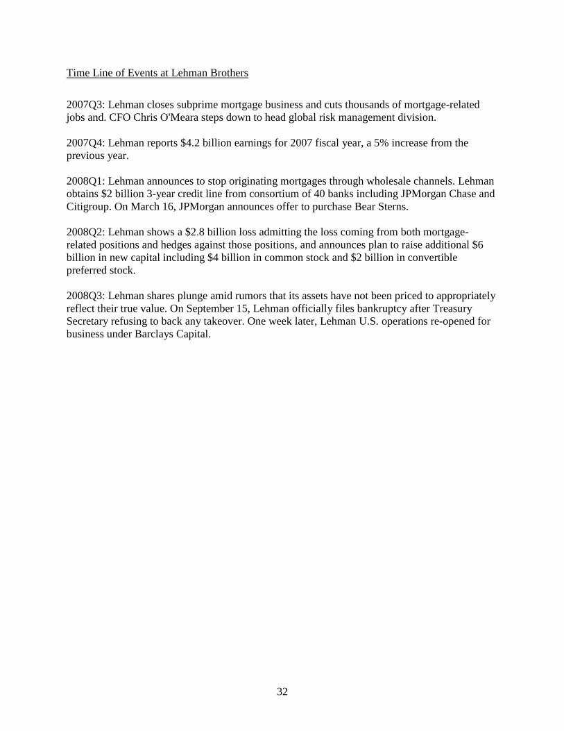
Time Line of Events at Lehman Brothers

2007Q3: Lehman closes subprime mortgage business and cuts thousands of mortgage-related

jobs and. CFO Chris O'Meara steps down to head global risk management division.

2007Q4: Lehman reports $4.2 billion earnings for 2007 fiscal year, a 5% increase from the

previous year.

2008Q1: Lehman announces to stop originating mortgages through wholesale channels. Lehman

obtains $2 billion 3-year credit line from consortium of 40 banks including JPMorgan Chase and

Citigroup. On March 16, JPMorgan announces offer to purchase Bear Sterns.

2008Q2: Lehman shows a $2.8 billion loss admitting the loss coming from both mortgage-

related positions and hedges against those positions, and announces plan to raise additional $6

billion in new capital including $4 billion in common stock and $2 billion in convertible

preferred stock.

2008Q3: Lehman shares plunge amid rumors that its assets have not been priced to appropriately

reflect their true value. On September 15, Lehman officially files bankruptcy after Treasury

Secretary refusing to back any takeover. One week later, Lehman U.S. operations re-opened for

business under Barclays Capital.

33

Table IX. Regression of a bank’s CoVaR on firm characteristics pre- and during crises


median state of the bank. The independent variables include 1-year lagged VaR of the bank and other firm characteristics such as maturity

mismatch, market to book, leverage, return volatility, total asset, loan to asset, commercial & industrial loan to total loan, non-interest income to interest income, non-interest income. The exact dates of economic crisis are taken from NBER web site. I define two time periods for each

economic contraction: boom period (1 calendar year) and crisis period (NBER’s definition of economic contraction).

Dependent Variable: CoVaRt Boom

1989Q4 – 1990Q3

Crisis

1990Q4 – 1991Q3

Boom

2000Q1 – 2000Q4

Crisis

2001Q1 – 2001Q4

Boom

2006Q4 – 2007Q3

Crisis

2007Q4 – 2008Q3

VaRt-1 0.00249

(0.11)

0.0426

(1.36)

-0.00131

(-0.10)

0.0241**

(2.37)

0.00140

(0.14)

0.0417**

(2.32)

Maturity Mismatch t-1 -1.848*

(-1.93)

-2.799*

(-1.86)

-0.0896

(-0.14)

0.316

(0.61)

0.0569

(0.12)

1.157

(1.29)

Market to Book t-1 0.397**

(2.15)

0.0722

(0.38)

-0.211***

(-3.60)

-0.121*

(-1.95)

-0.222***

(-3.65)

-0.320***

(-3.34)


(-0.10)

-0.0286

(-0.94)

-0.0192

(-1.28)

0.00296

(0.30)

-0.00253

(-0.16)

-0.0319

(-1.39)

Equity Return Volatility t-1 -0.225

(-0.02)

10.20

(1.04)

4.199

(1.08)

4.880

(1.59)

-9.444

(-1.40)

-8.326

(-0.70)

Log (Asset Size) t-1 -1.327

(-0.88)

-0.916

(-0.82)

-1.879***

(-6.15)

-1.924***

(-6.69)

-2.051***

(-7.47)

-2.928***

(-6.32)

Log (Asset Size) squared t-1 0.0381

(0.81)

0.0302

(0.82)

0.0571***

(5.79)

0.0581***

(6.24)

0.0602***

(7.16)

0.0826***

(5.90)

Loan to Total Asset t-1 0.461

(0.54)

0.765

(0.74)

-0.0418

(-0.10)

-0.00501

(-0.01)

-0.0118

(-0.04)

0.511

(0.89)


(-0.00)

-1.317

(-1.32)

-0.300

(-1.13)

-0.321

(-1.03)

-0.270

(-0.68)

-0.188

(-0.35)

Non-interest Income to Interest Income t-1

-2.991***

(-3.77)

-1.478

(-1.54)

-0.305

(-1.11)

-0.396

(-1.48)

-0.0455***

(-3.37)

-0.00167

(-0.06)

Intercept 9.818

(0.83)

6.381

(0.72)

14.60***

(6.06)

14.71***

(6.61)

16.81***

(7.44)

24.62***

(6.53)

N 216 232 909 976 971 895


F-test 4.97 4.28 14.08 11.75 42.56 11.53


10% respectively.

34

Table X. SES (Systemic Expected Shortfall) and non-interest income

The dependent variable is realized systemic expected shortfall (SES), which is the average equity return of the bank below its target level conditional on the average equity return of the entire banking system being below its target level. See Appendix B for technical details of SES’s

definition and implementation. The independent variables include bank characteristics such as maturity mismatch, market to book, leverage,

return volatility, total asset, loan to asset, commercial & industrial loan to total loan, return on asset, non-interest income to interest income, trading income to interest income, IBVC income to interest income, and other non-trading non-interest to interest income. Trading income

includes trading revenue, net securitization income, gain (loss) of loan sales and gain (loss) of real estate sales. IBVC income includes investment

banking/advisory fee, brokerage commission and venture capital revenue. Other non-trading non-interest income includes fiduciary income, deposits service charge, net servicing fee, service charges for safe deposit box and sales of money orders, rental income, credit card fees, gains on

non-hedging derivatives, and etc. All these detail accounting items are reported in FR Y-9C since 2001.

Dependent Variable: SES t (1) (2) (3) (4) (5)

Maturity Mismatch t -0.0739

(-0.664)

-0.00605

(-0.0416)

-0.0672

(-0.476)

-0.0371

(-0.262)

-0.0417

(-0.288)

Market to Book t 0.350***

(7.295)

0.432***

(30.02)

0.427***

(29.22)

0.436***

(30.74)

0.429***

(29.68)

Leverage t -0.0752***

(-5.571)

-0.0802***

(-27.68)

-0.0813***

(-27.20)

-0.0808***

(-27.84)

-0.0816***

(-27.21)

Equity Return Volatility t -11.98***

(-6.987)

-11.92***

(-4.770)

-11.77***

(-4.784)

-11.88***

(-4.763)

-11.56***

(-4.652)

Log (Total Asset) t -0.0323***

(-6.852)

-0.0236***

(-4.805)

-0.0239***

(-5.032)

-0.0200***

(-3.837)

-0.0215***

(-4.030)

Loan to Total Asset t -0.00581

(-0.111)

-0.129**

(-2.159)

-0.0893

(-1.568)

-0.0950

(-1.621)

-0.109*

(-1.817)

C&I Loan to Total Loan t 0.219***

(2.941)

0.178

(1.535)

0.164

(1.427)

0.189*

(1.659)

0.137

(1.163)

Return on Asset t 33.95

(1.534)

1.102

(0.566)

4.986**

(2.178)

1.269

(0.662)

5.388**

(2.212)

Non-interest Income to Interest Income t -0.0858**

(-2.036)

Trading Income to Interest Income t

-0.0990*

(-1.822)

-0.116**

(-2.027)

IBVC Income to Interest Income t

-0.0288***

(-4.112)

-0.0282***

(-3.840)

Other Non-trading Non-interest Income to

Interest Income t

-0.0908***

(-3.546)

-0.0297

(-1.133)

Intercept 1.684***

(6.652)

0.413***

(3.001)

1.598***

(7.965)

0.370***

(2.643)

1.564***

(7.575)

N 9,161 4,445 4,444 4,445 4,444

Adjusted R-square 0.65 0.69 0.70 0.70 0.70

F-test 430.07 139.85 142.83 141.09 136.41


10% respectively.

35

Table XI Robustness test: VaR and impact of differential lags

The dependent variable of regression (1) and (2) is individual bank’s VaR. The independent variables include one quarter lagged VaR and other firm characteristics including non-interest income to interest income and its breakdowns. Regression (3) to (5) use the 2-quarter, 3-quarter and 1-

year instead of 1-quarter lagged Non-interest/Interest Income ratio as independent variable.

Dependent Variable VaRt CoVaRt

(1) (2) (3) (4) (5)

VaRt-1 0.865***

(146.70)

0.898***

(102.20)

0.0419***

(8.95)

0.0419***

(8.94)

0.0419***

(8.95)

Maturity Mismatch t-1 -0.360

(-1.24)

-0.193

(-0.42)

-0.367**

(-2.07)

-0.367**

(-2.07)

-0.364**

(-2.05)

Market to Book t-1 0.0283

(1.04)

0.0549

(1.25)

-0.181***

(-8.70)

-0.181***

(-8.70)

-0.181***

(-8.69)


(-1.49)

-0.00812

(-0.71)

-0.00629

(-1.36)

-0.00624

(-1.35)

-0.00615

(-1.33)

Equity Return Volatility t-1 -17.18***

(-6.77)

-22.26***

(-4.90)

-0.00692

(-0.00)

-0.0145

(-0.01)

-0.0150

(-0.01)

Log(Total Asset) t-1 -0.0520

(-0.26)

-0.0773

(-0.27)

-1.348***

(-12.54)

-1.349***

(-12.54)

-1.350***

(-12.55)

Log (Total Asset)-squared t-1 0.000417

(0.07)

0.000229

(0.03)

0.0395***

(11.67)

0.0395***

(11.68)

0.0395***

(11.68)

Loan to Total Asset t-1 -0.0508

(-0.31)

-0.183

(-0.72)

0.476***

(3.93)

0.477***

(3.93)

0.480***

(3.95)


(-0.13)

-0.168

(-0.61)

-0.494***

(-5.12)

-0.495***

(-5.12)

-0.495***

(-5.12)

Trading Income to Interest Income t-1

-0.377

(-1.22)


-0.0255

(-1.35)

Other Non-trading Non-interest Income to Interest Income t-1

0.210

(1.32)

Non-interest Income to Interest Income t-1 -0.0211

(-1.41)


-0.0451***

(-10.48)


-0.0452***

(-10.35)


-0.0446***

(-9.96)

Intercept -2.854*

(-1.77)

1.239

(0.55)

10.11***

(11.31)

10.11***

(11.31)

10.12***

(11.31)

N 12,176 6,318 12,176 12,176 12,176


F-test 527.95 667.89 22.49 22.49 22.35

t-test is shown in the parenthesis with ***, ** and * indicating its statistical significant level of 1%, 5% and 10% respectively.

36

Table XII Robustness test: Non-interest income to total asset

The dependent variable is CoVaRt, which is the difference between CoVaR conditional on the bank being under distress and the CoVaR in the median state of the bank. The independent variables include one quarter lagged VaR of the bank and other firm characteristics such as maturity

mismatch, market to book, leverage, return volatility, total asset, loan to asset, commercial & industrial loan to total loan, return on asset, non-

interest income to total asset, trading income to total asset, IBVC income to total asset, and other non interest to total asset. Trading Income includes trading revenue, net securitization income, gain(loss) of loan sales and gain(loss) of real estate sales. IBVC Income includes investment

banking/advisory fee, brokerage commission and venture capital revenue. Other non-trading Income includes fiduciary income, deposits service

charge, net servicing fee, service charges for safe deposit box and sales of money orders, rental income, credit card fees, gains on non-hedging derivatives, and etc. All these detail accounting items are reported in FR Y-9C since 2001.

Dependent Variable: CoVaRt (1) (2) (3) (4) (5)

VaRt-1 0.0357***

(9.351)

0.0403***

(7.570)

0.0402***

(7.592)

0.0415***

(7.909)

0.0388***

(7.205)

Maturity Mismatch t-1 -0.368**

(-2.393)

0.145

(0.727)

0.0509

(0.258)

0.0828

(0.422)

0.103

(0.518)


(-10.10)

-0.204***

(-8.254)

-0.208***

(-8.225)

-0.203***

(-8.009)

-0.206***

(-7.921)

Leverage t-1 -0.00756*

(-1.879)

0.00436

(0.790)

0.00382

(0.683)

0.00412

(0.733)

0.00306

(0.540)

Equity Return Volatility t-1 4.352***

(3.973)

-0.616

(-0.322)

-0.564

(-0.293)

-0.748

(-0.387)

-0.186

(-0.0958)


(-15.69)

-0.136***

(-13.53)

-0.137***

(-13.48)

-0.135***

(-12.98)

-0.133***

(-12.82)

Loan to Total Asset t-1 -0.206**

(-2.199)

-0.308**

(-2.378)

-0.236*

(-1.863)

-0.257**

(-2.037)

-0.292**

(-2.247)

C&I Loan to Total Loan t-1 -0.324**

(-2.462)

-0.691***

(-3.383)

-0.673***

(-3.294)

-0.641***

(-3.153)

-0.733***

(-3.574)

Return on Asset t-1 -1.352

(-0.445)

-7.642***

(-3.787)

-3.648

(-1.026)

-8.024***

(-4.071)

-2.302

(-0.589)

Non-interest Income to Total Asset t-1 -4.027***

(-5.396)

Trading Income to Total Asset t-1

-6.125**

(-2.123)

-7.082**

(-2.381)

IBVC Income to Total Asset t-1

-2.296**

(-2.478)

-2.582***

(-2.645)

Other Non-trading Non-interest Income to Total Asset t-1

-2.071

(-0.643)

-1.433

(-0.448)

Intercept 1.204***

(6.786)

0.247

(1.047)

0.249

(1.055)

1.998***

(10.85)

0.199

(0.841)

N 15,825 7,982 7,981 7,988 7,981


F-test 45.26 58.95 59.06 59.06 56.50


10% respectively.

37

Table XIII Robustness test: Regression of a bank’s CoVaR on non-interest income of the

same quarter


median state of the bank. The independent variables include the current quarter’s VaR and other firm characteristics such as maturity mismatch, market to book, leverage, return volatility, total asset, loan to asset, commercial & industrial loan to total loan, non-interest to interest income,

trading income to interest income, IBVC income to interest income, and other non-trading non-interest income to non-interest income ratios.

Trading Income includes trading revenue, net securitization income, gain(loss) of loan sales and gain(loss) of real estate sales. IBVC Income includes investment banking/advisory fee, brokerage commission and venture capital revenue. Other Non-trading Income includes fiduciary

income, deposits service charge, net servicing fee, service charges for safe deposit box and sales of money orders, rental income, credit card fees,

gains on non-hedging derivatives, and etc.


VaRt 0.0501***

(12.28)

0.0493***

(12.16)

0.0485***

(11.91)

0.0477***

(11.78)

0.0461***

(8.391)

0.0449***

(8.257)

Maturity Mismatch t -0.359**

(-2.351)

-0.320**

(-2.068)

-0.382**

(-2.513)

-0.343**

(-2.228)

0.0953

(0.501)

0.289

(1.523)

Market to Book t -0.197***

(-10.47)

-0.172***

(-9.146)

-0.199***

(-10.53)

-0.174***

(-9.206)

-0.207***

(-8.421)

-0.165***

(-6.863)

Leverage t -0.00541

(-1.395)

-0.00429

(-1.110)

-0.00634

(-1.629)

-0.00521

(-1.342)

0.00452

(0.844)

0.00346

(0.654)

Equity Return Volatility t 5.220***

(4.815)

2.448**

(2.228)

5.593***

(5.148)

2.821**

(2.561)

0.754

(0.417)

-0.643

(-0.361)

Log (Total Asset) t -0.123***

(-17.10)

-1.375***

(-16.83)

-0.118***

(-16.48)

-1.369***

(-16.87)

-0.126***

(-13.45)

-1.547***

(-14.60)

Log (Total Asset) squared t

0.0400***

(15.33)

0.0400***

(15.43)

0.0451***

(13.64)

Loan to Total Asset t -0.197**

(-2.213)

-0.133

(-1.468)

-0.176**

(-1.979)

-0.112

(-1.243)

-0.284**

(-2.387)

-0.202*

(-1.667)

C&I Loan to Total Loan t -0.248*

(-1.931)

-0.318**

(-2.477)

-0.300**

(-2.330)

-0.369***

(-2.872)

-0.722***

(-3.657)

-0.663***

(-3.375)

Return on Asset t -9.272***

(-5.061)

-9.657***

(-5.470)

-4.160*

(-1.958)

-4.595**

(-2.159)

-2.171

(-0.877)

-2.990

(-1.231)

Non-interest Income to Interest Income t

-0.0472***

(-9.241)

-0.0468***

(-8.552)

Trading Income to Interest Income t

-0.264*

(-1.698)

-0.308**

(-1.997)

IBVC Income to Interest Income t

-0.0420***

(-6.724)

-0.0350***

(-5.553)

Other Non-trading Non-interest Income t

-0.0245

(-0.0450)

-0.521

(-0.884)

Intercept 1.375***

(8.170)

11.11***

(17.23)

1.294***

(7.703)

11.01***

(17.17)

1.217***

(6.177)

12.71***

(15.31)

N 15,825 15,825 15,825 15,825 7,981 7,981


F-test 17.82 22.31 20.41 24.43 34.16 38.40


10% respectively.

38

Table XIV Robustness test: Statistics of banks drifting between non-interest income terciles

The number of banks whose Non-interest Income to Interest Income ratios change from one tercile to another tercile in each calendar quarter.

Year Quarter # Changes # TotalBanks #

#

Changes

TotalBanks

Year Quarter # Changes # TotalBanks

#

#

Changes

TotalBanks

1986 4 1 49 2% 1998 1 5 206 2%

1987 1 2 50 4% 1998 2 13 196 7%

1987 2 2 50 4% 1998 3 6 208 3%

1987 3 1 53 2% 1998 4 2 215 1%

1987 4 2 54 4% 1999 1 7 223 3%

1988 1 1 53 2% 1999 2 11 227 5%

1988 2 4 55 7% 1999 3 5 221 2%

1988 3 2 56 4% 1999 4 9 228 4%

1988 4 1 57 2% 2000 1 9 233 4%

1989 1 1 57 2% 2000 2 21 229 9%

1989 2 0 55 0% 2000 3 11 232 5%

1989 3 0 56 0% 2000 4 9 235 4%

1989 4 0 58 0% 2001 1 8 247 3%

1990 1 0 59 0% 2001 2 26 241 11%

1990 2 3 57 5% 2001 3 8 225 4%

1990 3 3 55 5% 2001 4 8 227 4%

1990 4 2 62 3% 2002 1 9 185 5%

1991 1 3 63 5% 2002 2 14 200 7%

1991 2 4 62 6% 2002 3 6 244 2%

1991 3 2 67 3% 2002 4 4 252 2%

1991 4 1 77 1% 2003 1 11 271 4%

1992 1 0 77 0% 2003 2 14 258 5%

1992 2 8 78 10% 2003 3 8 257 3%

1992 3 4 79 5% 2003 4 3 266 1%

1992 4 3 79 4% 2004 1 2 269 1%

1993 1 0 79 0% 2004 2 21 266 8%

1993 2 4 79 5% 2004 3 8 258 3%

1993 3 4 82 5% 2004 4 4 253 2%

1993 4 0 81 0% 2005 1 6 248 2%

1994 1 6 82 7% 2005 2 10 248 4%

1994 2 4 82 5% 2005 3 12 249 5%

1994 3 7 135 5% 2005 4 4 257 2%

1994 4 4 142 3% 2006 1 7 251 3%

1995 1 3 142 2% 2006 2 23 238 10%

1995 2 13 146 9% 2006 3 8 244 3%

1995 3 5 148 3% 2006 4 6 234 3%

1995 4 7 155 5% 2007 1 5 237 2%

1996 1 6 150 4% 2007 2 13 226 6%

1996 2 6 164 4% 2007 3 8 225 4%

1996 3 4 164 2% 2007 4 7 217 3%

1996 4 4 166 2% 2008 1 7 217 3%

1997 1 2 161 1% 2008 2 14 221 6%

1997 2 12 176 7% 2008 3 12 222 5%

1997 3 8 180 4% 2008 4 10 216 5%

1997 4 6 195 3% Mean 4%

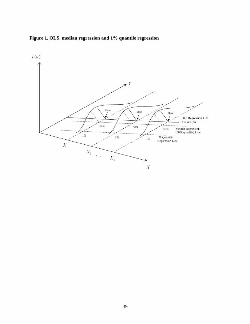
39

Figure 1. OLS, median regression and 1% quantile regression

banks non-interest income and systemic riskmarkus/research/papers/covar_non...banks’ non-interest...

Documents