bap: basic strong-motion accelerogram processing software; version … · united states department...
TRANSCRIPT

Open-File Report
92-296A
BAP: Basic Strong-Motion Accelerogram Processing
Software; Version 1.0
April M. Converse and A. Gerald Brady
United States Department of the Interior
Geological Survey


UNITED STATES DEPARTMENT OF THE INTERIOR U.S. GEOLOGICAL SURVEY
BAP: Basic Strong-Motion Accelerogram Processing Software
Version 1.0
by April M. Converse
with Chapter 5 by
April M. Converse and A. Gerald Brady
Open-File Report 92-296A
01 March 92
This report is preliminary and has not been reviewed for conformity with U. S. Geological Survey editorial standards. Any use of trade, product, or firm names is for descriptive purposes only and does not imply endorsement by the USGS. Although this software has been used by the U.S. Geological Survey, no warranty, expressed or implied, is made by the USGS as to the accuracy and functioning of the software and related material, nor shall the fact of distribution constitute any such warranty, and no responsibility is assumed by the USGS in connection therewith.

Version 1.0
Open-File Reports are Distributed by:
Books and Open-File Reports Section U.S. Geological Survey
Box 25425, Federal Center Denver, Colorado 80225
(303) 236-7476
Version 1.0
i
Table of Contents Preface iii Acknowledgments iv Chapters 1.0 Introduction 1-1 1.1 Time-Series Data Files 1-1 1.2 Computers 1-2 1.3 PCs 1-2 1.4 Abbreviations and typographic conventions used in this report 1-3 1.5 Running BAP 1-3 2.0 BAP Processing Steps 2-1 2.1 INPUT 2-2 2.2 INTERP: Interpolation 2-2 2.3 LINCOR: Linear Corrections 2-2 2.4 PAD: Add Leading and Trailing Zeros 2-3 2.5 INSCOR: Instrument Correction 2-4 2.6 HICUT: High-Cut Filter 2-4 2.7 DECIM: Reduce Sampling Rate 2-4 2.8 LOCUT: Low-Cut Filter 2-5 2.9 AVD: Calculate Velocity & Displacement 2-6 or Acceleration & Displacement 2.10 FAS: Fourier Amplitude Spectrum 2-7 2.11 RESPON: Response Spectra 2-7 3.0 BAP Input/Output files 3-1 3.1 Input Files 3-1 3.2 Output Files 3-1 4.0 BAP Run Parameters 4-1 4.1 Sample BAP Commands and Run Parameter Settings 4-1 4.2 Commands that Require More than One Line 4-3 4.3 Default Run Parameter Settings 4-3 4.4 Run Parameter Assignment Statements 4-5 4.5 Processing Step Names in Run Parameter Lists 4-6 4.6 Parameter Names and Assignment Values 4-7 5.0 Guidelines for Selecting BAP run Parameters 5-1 5.1 Interpolation, Decimation, and Alias Errors 5-3 5.2 Instrument Correction & High-Cut Filter Parameters 5-4 5.3 Pre-filter Pads 5-8 5.4 Tapers 5-11 5.5 Velocity and Displacement 5-13 5.6 Low-Cut Filter Corners 5-13 5.7 Filter Transitions 5-15 5.8 Fourier Amplitude Spectra 5-16 5.9 Response Spectra 5-17 5.10 Some Sample Command Lines 5-18 5.11 Run Messages 5-19

Version 1.0
ii
6.0 Support Programs 6-1 7.0 Plots 7-1 7.1 Plotting Programs 7-1 7.2 Screen Plots 7-2 7.3 Plotting on Computers other than PCs 7-2 7.4 TSPLOT, Time-Series Plotting Program 7-3 Appendixes A. Quick Reference A-1 B. Two Sample BAP Runs B-1 B.1 Commands for First Example B-2 B.2 Commands for Second Example B-4 B.3 Results from the First Example B-6 B.4 Results from the Second Example B-12 C. Run-Time Comparisons C-1 D. Acquiring BAP software D-1 E. Installing BAP on IBM personal computers E-1 E.1 Installation Overview E-2 E.2 Installation Steps E-3 E.3 Test Runs E-9 E.4 Archived Distribution Files E-12 E.5 Unarchived Distribution Files E-13 F. Trouble Shooting F-1 F.1 Run Messages F-1 F.2 Disk Space F-1 F.3 RAM Space F-2 F.4 Extended RAM on PCs F-2 F.5 The infile Parameter in BAPʹs Run Parameter List F-5 F.6 Using & and @ in Long Command Lines F-6 F.7 File Names F-6 F.8 BAP Output Files F-7 F.9 PC Screen-Plotting Programs F-7 F.10 The PC/DOS ʺagrootʺ Environment Variable F-7 F.11 The Size of the DOS ʺEnvironment Spaceʺ on PCs F-7 F.12 Technical Support F-9 G. Programming Considerations G-1 G.1 SCATTR and GATHER G-1 G.2 Programming for PCs G-3 G.3 Computers other than PCs G-4 G.4 Plotting Code G-5 G.5 Sample Code G-6 G.6 Programming Notes G-6

Version 1.0
iii
H. Fortran Code H-1 H.1 Include files H-4 H.2 BAP2.FOR H-8 H.3 BAPSPS.FOR H-16 H.4 BAPPAD.FOR H-18 H.5 FDIC.FOR H-22 H.6 BIHIP.FOR H-30 H.7 BAPFAS.FOR H-32 H.8 BAPRSC.FOR H-36 H.9 CMPMAX.FOR H-38 References & Bibliography R-1

Version 1.0
iv
Preface
This report describes one of the computer programs used at the U.S. Geological Survey (USGS) for processing digitized strong-motion accelerograms. The program, named BAP, can process time series data files from the Strong-Motion CD-ROM that is available from the USGS (Reference [20], by Seekins and others). Consequently, the BAP program should provide useful data processing functions to organizations outside the USGS that have acquired that CD-ROM. This report is a userʹs guide for members of the USGS who use the software as well as for members of other organizations who acquire the software from the USGS. BAP is a new, preliminary program. All the computing subroutines, those listed in Appendix H, have been thoroughly tested, but the overhead subroutines have not. BAP users are encouraged to mail the author evidence of any problems or inconveniences encountered while running BAP. 01 March 1992 April Converse ES&G Data Project (BAP) U.S. Geological Survey, Mail Stop 977 345 Middlefield Road Menlo Park, CA, 94025-3591 USA Telephone: (415) 329-5666 FAX: (415) 329-5163

Version 1.0
v
Acknowledgments This report and the software it describes result from the cooperative efforts of many members of the USGS. Some of the Fortran subroutines that make up the program were written by authors from organizations other than the USGS. These subroutines are used in BAP with permission. They were written by I.M. Idriss while at the University of California at Berkeley; Keith McCamy while at Lamont-Doherty Geological Observatory; Norman Brenner while at MIT Laboratory; and the authors of the textbook Numerical Recipes (Reference [18]). All of the software tools used to construct BAP and its support programs on VAX computers were provided by the VAX/VMS operating system. Software from several sources was used to construct the PC versions of the programs, however. The PC software packages employed for the effort were: the Microsoft Fortran Compiler; the Lahey F77L-EM/32 Fortran compiler; the Ergo/OS Dos Extender; the ForWarn static Fortran syntax analyzer by Quibus, Inc.; the PKZIP file compression software by PKWARE, Inc.; and the Norton AntiVirus software by Peter Norton Computing, Inc. This report was formatted with the Microsoft WORD software for PCs.


BAP page 1-1 01mar92 Introduction
Version 1.0
Chapter 1
Introduction The BAP computer program can be used to process and plot digitized strong-motion earthquake records. BAP will calculate velocity and displacement from an input acceleration time series or it will calculate acceleration and displacement from an input velocity time series. The program will make linear baseline corrections, apply instrument correction, filter high frequency and/or low frequency content from the time series, calculate the Fourier amplitude spectrum, and calculate response spectra. It will also plot the results after each processing step. BAP is one of a group of programs, the AGRAM programs1, that were developed at the USGS to process digitized analog strong-motion records. Digitally recorded data, after preliminary processing unique to each recording device, can also be processed by BAP. 1.1 Time-Series Data Files BAP reads its input time series from a disk file that must be in one of two formats: "SMC" format or "BBF" format. The SMC format is that used for the time series files stored on the Strong-Motion CD-ROM available from the USGS2. The BBF format is the blocked-binary file format used for most of the time series data files in the Engineering Seismology and Geology data collection at the USGS in Menlo Park. More information about the time-series data files is given in Chapter 3 and details about the two file formats are given in the smcfmt.doc and bbffmt.doc documentation files that are included among the BAP software distribution files. Those who are willing to reprogram some of the Fortran code used to implement BAP can modify the program so it will accept input files in other formats. Several of the support programs (IMPORT, EXPORT, and BBDATA) discussed in Chapter 6 perform data file reformatting functions and they too could be modified to handle other formats. Refer to Appendix G for programming guidelines. 1 Reference [7], by Converse (1984). 2 Reference [20], "Digitized Strong-Motion Accelerograms of North and Central American
Earthquakes 1933-1986", by Seekins and others, is a CD-ROM that contains more than 4,000 time-series data files. CD-ROMs are read-only compact disks that can be read by a computer, provided a CD-ROM reader is installed on the computer. The disks are the same as those used for compact-disk musical recordings.
page 1-2 BAP Introduction 01mar92
Version 1.0
1.2 Computers BAP has been installed and tested on VAX computers running the DEC VMS operating system (version 5.4) and on IBM-style, 80386, personal computers running the Microsoft DOS operating system (version 3.3). See Appendix C for a table that indicates the time it takes to run the BAP examples shown in Appendix B on several different computers. BAP and its support programs are available for PCs as executable files and as Fortran files; they are available only as Fortran files for other computers. See Appendix D for distribution information. BAP is coded in Fortran that conforms to the ANSI Fortran 77 standard. Consequently, BAP should be transportable to any computer having a "full" Fortran 77 compiler. Preliminary guidelines for modifying the BAP code and for transporting BAP to computers other than VAXes or PCs are given in Appendix G. More detailed guidelines are given in the progbap.nts and progagram.nts files included among the BAP software distribution files. 1.3 PCs The executable files included among the PC software distribution files require an IBM-style PC or "clone" having: ∙ an 80386 or and upward-compatible CPU such as an 80486; ∙ an 80387 math coprocessor; ∙ a hard disk with 10M bytes or more available; ∙ a 1.44M byte, 3.5" floppy disk drive (for the distribution diskettes); ∙ 3M bytes or more of RAM; ∙ DOS version 3.3 or greater; ∙ a PostScript printer or PostScript-to-other-printer translating software; and ∙ a text editor (the "EDIT" editor that comes with DOS 5.0 will do) or a word
processor that will create and edit character-only files. Fortran files as well as executable files are included among the PC/BAP software distribution files so those who wish to tailor the software for their own computer or their own needs may do so. The PC version of BAP, as distributed in executable form, uses "DOS extending" software to access memory above the 640K DOS-imposed memory limit. The DOS extender used is "Ergo OS/386" as provided with the "Lahey F77L-EM/32" Fortran compiler. BAP and OS/386 do not require additional memory management software, but they are compatible with any expanded-memory-managing software packages that comply with the VCPI standard. These include, but are not limited to: ∙ 386MAX (version 4.0 or higher) ∙ QEMM (version 4.2 or higher) ∙ CEMM (version 6.0 or higher) BAP and Ergo OS/386 are compatible with Quarterdeck's "DESQview" multitasking software, but they are not compatible with Microsoft "Windows". (A Windows-compatible version of BAP might be provided with future versions of the BAP distribution files if users indicate a need for such.)

BAP page 1-3 01mar92 Introduction
Version 1.0
1.4 Abbreviations and Typographic Conventions used in this Report Throughout this report, the term "VAX" is used to refer to a VAX computer running the VMS operating system, and the term "PC" is used to refer to an IBM-style 80386 personal computer running the IBM PC-DOS or the Microsoft MS-DOS operating system. Two typefaces are used in this report. This typeface is used for normal text and this typeface is used to represent characters that one might see on the computer screen or in computer print-outs. The computer typeface is frequently mixed in with normal text to emphasize words that can be used as BAP run parameters (e.g., infile, infmt, eda.r01, bbf ) or words that represent operating-system level commands (e.g., bap, scrplot, print). Underlined italics (underlined italics) are used to indicate names of items the user should supply. And doubly-underlined italics (doubly-underlined italics) are occasionally used in Chapter 7 (about plots) and Appendix A (the quick-reference Appendix) to indicate names of items the user must supply, as distinct from singly-underlined items that the user may choose whether to supply or not. The prompt from the VAX/VMS operating system is shown as vax$; the prompt from the PC/DOS operating system is shown as dos>; and a generic computer prompt is shown as $|>. The generic prompt indicates that the sample command that follows would have the same effect on a PC as on a VAX. For instance, the following line illustrates a type command that a user might enter in response to the prompt from the PC/DOS operating system: dos> type \agram\docs\smcfmt.doc The type command, which is available in DOS and in VMS, is used to display the contents of a text file on the user's screen. The corresponding command on a VAX/VMS computer would be: vax$ type [agram.docs]smcfmt.doc And the following command would work on either computer, provided that the smcfmt.doc file were located in the user's current disk directory: $|> type smcfmt.doc PC/DOS path name conventions are usually used in this report rather than the VAX conventions except where command lines that would work on a VAX but not on a PC are shown. The file and directory hierarchy for the BAP distribution files should be the same on both types of machines, only the characters used to describe the hierarchy would be different. The PC/DOS operating system requires directory paths to be expressed with backslash characters separating directory names and file names, while the VAX/VMS operating system requires brackets and dots. For example, the smcfmt.doc file should be found in a directory named docs under a directory named agram. The path name for the file on a PC would be: \agram\docs\smcfmt.doc and on a VAX it would be: [agram.docs]smcfmt.doc.
1.5 Running BAP The user indicates the processing steps BAP should perform on the command line used to invoke the program. Such information is referred to as the "run parameters" throughout this report. The run parameters may be given on the
page 1-4 BAP Introduction 01mar92
Version 1.0
command line or they may be given in a separate text file, the name of which is then given on the BAP command line. The name of a file that contains run parameters is prefaced by an "@" character on the BAP command line to distinguish a run-parameters file from an input time-series data file. Here are some examples of valid BAP command lines: $|> bap $|> bap tsdata.smc $|> bap @doit.brp $|> bap tsdata.smc, @smc.brp, corner=0.13 $|> bap infile=tsdata.smc, inscor, & locut(f),corner=0.13, avd(f), fas(p) done $|> bap bapacc.bbf, respon(f,p) $|> bap show A description of each of these commands is given in Section 4.1 of Chapter 4. All of the BAP run parameters are described in Chapter 4, the processing steps are described in Chapter 2 and guidelines for running BAP are given in Chapter 5.
BAP page 2-1 01mar92 Processing Steps
Version 1.0
Chapter 2
BAP Processing Steps The BAP processing steps, the names by which each is indicated in a BAP run-parameters list, and the order in which they are performed are: Step Name Process INPUT Read the run parameters and the input time series data file. INTERP Linearly interpolate an input time series given as unevenly-sampled
(x,y) pairs to evenly-sampled y-values. This step is required for an unevenly-sampled input series because all the subsequent processing steps require an evenly-sampled series. This step is not required for input time series, such as those that come from the Strong-Motion CD-ROM1, that are already evenly-sampled at the desired sampling rate.
LINCOR Subtract a straight line from the input time series. The line can be the linear least-squares fit to the time series, the mean value of the time series, or a user-specified constant. This step will not be required for input files, such as those from the USGS, that have already had similar processing applied. It will be required for some of the files on the Strong-Motion CD-ROM that did not originate at the USGS, however. Other linear corrections may be applied in the AVD step.
PAD Add leading and trailing zeros to the time series, in preparation for the HICUT and LOCUT filters.
INSCOR Instrument correct to compensate for the diminishing response of a damped, spring-mass, single-degree-of-freedom, optical-mechanical accelerometer (hereinafter referred to as a "spring-mass accelerometer") at higher frequencies, and apply the HICUT filter.
HICUT Apply a frequency-domain filter to remove high-frequency content from the time series. The filter is normally applied as part of the INSCOR step, but it can be requested as a separate step when the INSCOR step is not used.
DECIM Reduce the sampling rate by removing all but the first of each 3 (or ndense) samples. This step will not be required for input files
1 Reference [20], by Seekins and others.

page 2-2 BAP Processing Steps 01mar92
Version 1.0
that come from the Strong-Motion CD-ROM. It should only be used on very densely digitized data.
LOCUT Apply a bidirectional Butterworth filter to remove low frequency content from the time series.
AVD Integrate the acceleration time series once to calculate a velocity time series, twice to calculate a displacement time series. Or, if the input time series represents velocity rather than acceleration, differentiate the velocity time series to calculate an acceleration time series and integrate the velocity to calculate displacement.
FAS Calculate the Fourier amplitude spectrum of acceleration. RESPON Calculate response spectra at several specified damping ratios. The processing steps are described in further detail in the paragraphs that follow and guidelines for using each step are given in Chapter 5 along with warnings about their limitations and side effects. The BAP run-parameter names used in these descriptions are fully described in Chapter 4. Run-parameter names (e.g., infmt) and assignment statements (e.g., infmt =bbf) are shown in the computer typeface (this typeface). 2.1 INPUT The INPUT processing step reads the run parameters and the input time-series data file. 2.2 INTERP: Interpolation The INTERP processing step linearly interpolates an input time series that was given as a series of (x,y) pairs to a series of evenly-sampled y-values. The INTERPolation is required for an unevenly-sampled input series because all the subsequent processing steps require an evenly-sampled series. The INTERP step will also linearly interpolate an evenly-sampled input time series to a denser sampling interval (in which case, the HICUT filter should also be applied -- see Section 5.1 in Chapter 5). 2.3 LINCOR: Linear Corrections The LINCOR processing step subtracts a straight line from the input time series. The line can be the linear least-squares fit to the time series, the mean value of the time series, or a user-specified constant. This step is often unnecessary because the reference trace, then the mean value of the resulting data trace, have usually been subtracted from each data trace during the preliminary processing of a digitized analog record. Some of the time series on the Strong-Motion CD-ROM came from analog records that had no reference trace, however, and these may contain linear trends that can be removed with the LINCOR step. When the linear least-squares fit or the mean value is used in the LINCOR step, the linear fit or mean value is, by default, calculated from the entire time series. By using the begfit and endfit run parameters, however, the user can request that only a portion of the wave-form be used to calculate the line or mean value to be subtracted from the time series. For example, a digitally recorded time series often needs to have the average offset of the pre-event portion of the time series subtracted from the entire time series: to accomplish this, begfit and endfit can be set to bracket just the pre-event portion.

BAP page 2-3 01mar92 Processing Steps
Version 1.0
When a linear least-squares fit, a mean value, or a constant is subtracted from the time series, the line or constant is, by default, subtracted from every sample in the time series. The beglin and endlin run parameters, however, can be used to indicate the end points of just a section of the time series from which the line or constant should be subtracted. These two run parameters will rarely be required, but they might be used, for instance, with the processing technique discussed in reference [12], by Iwan and others. Other linear corrections may be applied in the AVD step. As part of the AVD process, the user may request that the linear least-squares fit of the velocity be subtracted from the velocity time series and that the slope of the fit line be subtracted from the acceleration time series.
2.4 PAD: Add Leading and Trailing Zeros The PAD processing step extends the time series in both directions by adding leading and trailing zeros in preparation for the HICUT and LOCUT filters. Acausal filters, such as those applied in the HICUT and LOCUT steps, produce output time series that have non-zero values for times beyond those in the input series. The non-zero leading and trailing values should be included in the integrations used in the AVD step, in the Fourier amplitude calculations in the FAS step, and in the response spectra calculations in the RESPON step. If they are ignored, the result is to reintroduce frequencies that were removed by the filter. By default, when the user does not indicate the pad length via the padsec parameter, BAP will choose the length based on the transition band parameters, corner and nroll, used in the LOCUT processing step. The pad length, in seconds, will be 1.5*nroll/corner. This means that in a typical case where nroll=1 and corner=0.1, each pad will be 15 seconds long. As there are two pad areas, one increasing the length of a time series at its beginning, and another at the end, there will be 30 seconds of padding added in this case. At 200 samples per second, the time series will be extended by 6,000 points and by much more than that if nroll is greater than 1 or corner is less than 0.1. The default pad length, 1.5*nroll/corner, may not be adequate for some records. The user should inspect plots of the padded, filtered acceleration and plots of the velocity and displacement calculated from that acceleration to verify that the pad lengths used were sufficiently long. Figures 5.3.a and 5.3.b in Chapter 5 illustrate the effect of using pads of insufficient lengths. Pad lengths required by the LOCUT filter are much larger than those required by the HICUT filter, so BAP usually does the padding in two steps. Short, two-second-duration pads are added before the INSCOR (or HICUT) step, then the pads are extended before the LOCUT step. Otherwise, the INSCOR (or HICUT) step would take an unnecessarily long while to process an unneccessarily long time series. The padding sequence can be modified via the jpad run parameter, however. Refer to Section 4.6 of Chapter 4 for information about jpad. If the first or last point of the input time series is significantly different from zero, there will be a sharp offset in the padded time series where the input samples meet the pad area. This offset will introduce spurious frequencies ("leakage") into the series if either of the filters (HICUT or LOCUT) is applied. The ktaper and tapsec run parameters may be used to minimize the effect of such an offset. When

page 2-4 BAP Processing Steps 01mar92
Version 1.0
ktaper=on, a cosine taper, tapsec seconds long, will be applied at both ends of the time series. When ktaper=zcross, time series samples before the first zero crossing and after the last zero crossing will be reset to zero. By default, ktaper=zcross; if no tapering is required, the user should reset ktaper to off. Refer to Section 4.6 of Chapter 4 and Section 5.4 of Chapter 5 for information about ktaper and tapsec. Figure 5.4.a in Chapter 5 illustrates the ktaper options.
2.5 INSCOR: Instrument Correction The INSCOR processing step makes a correction to the time series to compensate for the diminishing response of a spring-mass accelerometer at higher frequencies. The instrument-correcting algorithm is based on the second-order differential equation representing motion of a single-degree-of-freedom, damped, harmonic oscillator (see page 46 of reference [11]): ai = zi + zi' * 2 * ζ/ω + zi"/ω2 Where: ai is the corrected time series; zi is the uncorrected, equally sampled, time series; zi' is the first derivative of zi; zi" is the second derivative of zi; ζ is the damping of the recording instrument, as a fraction of critical
damping; and ω is the natural frequency of the recording instrument in radians per
second. Whenever the INSCOR processing step is requested, the HICUT processing step is also applied, to remove high-frequency noise that is amplified by the instrument correction. Note that the INSCOR processing step is intended for time series that were recorded with spring-mass accelerometers and is not suitable for use with time series recorded by other types of transducers. See Section 5.2 of Chapter 5 for more information about when the instrument correction step is required and when it is not appropriate.
2.6 HICUT: High-Cut Filter The HICUT processing step applies a filter to remove high frequency content from the time series. The time series is transformed to the frequency domain by a fast Fourier transform (FFT), the same transformation used for the INSCOR step. The high-cut filter is applied by setting samples in the frequency domain to zero above hitend Hz and weighting the samples between hitbeg and hitend Hz with a cosine half-bell taper. Hitbeg=50 and hitend=100 in the default case. After instrument correction (if it were requested) and filtering, the transform is inverted back to the time domain. The HICUT filter is normally applied as part of the INSCOR step, but it can be requested as a separate step when the INSCOR step is not used.

BAP page 2-5 01mar92 Processing Steps
Version 1.0
2.7 DECIM: Reduce sampling rate The DECIM processing step reduces the sampling rate by removing all but the first of each ndense samples. The decimation is done at this point in the processing, between the INSCOR/HICUT step and the LOCUT step, rather than in the INTERP interpolation so that the derivatives required in the INSCOR step can be calculated as accurately as the data will allow. This step will rarely be required for other than the records digitized by the automatic trace-following laser digitizer2 employed by the USGS, which are digitized at approximately 600 samples per second. The HICUT filter should be applied whenever DECIMation is used: See Section 5.1 in Chapter 5.
2.8 LOCUT: Low-Cut Filter The LOCUT processing step applies a bidirectional Butterworth filter to remove low frequency content from the time series. Although some accurately recorded, accurately digitized records will not require the LOCUT processing, many records will require that long periods contaminated by noise be filtered from the time series before reasonable displacements or response spectra can be calculated. Users must consider for each record whether or not filtering is required. See Chapter 5, Section 5.6 for low-cut filter guidelines. The transition of the filter is indicated in the BAP run parameters with a frequency, corner, that indicates where in the frequency spectrum the transition between the pass band and the stop band of the filter should occur, and a roll-off parameter, nroll, that controls the steepness of the transition. Corner is the frequency, in Hz, in the transition band where the Fourier amplitude is reduced to one-half by filtering. By default, nroll=1 and corner=* (where "*" indicates "undefined"). The user or the input file must provide a corner value if the LOCUT step is to be performed. The Fourier amplitude transfer function of the bidirectional Butterworth filter, Tbi, is given by: Tbi( f ) = 1 / [1 + (corner/f)4*nroll] where the independent variable, f, is frequency in Hz. The roll-off parameter nroll is equal to half of what is often called the "order" of a Butterworth filter in conventional terminology. The exponent in the transfer function equation shown above would be 2N rather than 4*nroll if it were expressed in terms of a Butterworth "order", N. The number of "poles" in the filter is 4*nroll. The LOCUT filter is implemented with a different algorithm than the HICUT filter for several reasons, the primary reason being historical: BAP evolved from earlier software in which the two filters were implemented in separate programs. The predecessor software was intended for use with the densely-digitized records processed by the USGS, for which the sampling rate is reduced from 600 to 200
2 The automatic trace-following laser digitizer used for many USGS-processed
records is operated by LS Associates; 1707 Lafayette Street, Suite B; Santa Clara, CA 95050 USA.

page 2-6 BAP Processing Steps 01mar92
Version 1.0
samples per second between the two filters. The low-cut filter requires much longer pads than does the high-cut filter, so applying the filters in separate steps allows the combined INSCOR and HICUT processing to be applied to a padded time series that is shorter than would be required if the LOCUT filter were applied concurrently, thus saving processing time. Applying the LOCUT filter after DECIMating the sampling rate from 600 to 200 samples per second reduces the number of samples that the LOCUT filter would otherwise need to process, again saving processing time. Also, the high-cut filter used here is applied in the frequency domain as part of the instrument-correcting step and as a consequence requires very little additional processing. The low-cut filter cannot be applied in the same process, however, because the instrument correction and high-cut filter are applied to successive segments of the time-series, and each segment (3072 samples) is shorter than the periods affected by the low-cut filter. The bidirectional Butterworth filter algorithm was selected for the low-cut filter because of its zero phase-shift and its flat response in the pass band.
2.9 AVD: Calculate Velocity & Displacement or Acceleration & Displacement
The AVD processing step results in three separate time series: acceleration, velocity, and displacement. If, as is usually the case, the input time series represents the acceleration of a recording instrument, the corrected input acceleration time series will be integrated twice in the AVD step: once to calculate a velocity time series, twice to calculate a displacement time series. If, as is the case with some digitally recorded data, the input time series represents velocity rather than acceleration, the AVD processing step will differentiate the velocity time series to approximate an acceleration time series and will integrate the velocity to calculate displacement. Integration is performed using the trapezoidal method and using zero as the initial velocity and initial displacement. The pads are included in the integration bounds. vi = vi-1 + ( ai-1 + ai ) * ∆t/2 di = di-1 + ( vi-1 + vi ) * ∆t/2 The acceleration time series, when determined from an input velocity time series, is calculated by a simple 2-point numerical differentiation: ai = ( vi - vi-1 )/ ∆t This derivative might not be accurate enough for some purposes, depending on the sampling rate and the frequency content of the signal. (Future versions of BAP may provide more accurate algorithms for calculating the AVD derivatives and integrals.) Additional processing occurs between the two integrations when velfit=on (it is off by default), when the input time series is acceleration, and when no padding or low-cut filter is applied (padsec=0.0 and NOlocut). A fitted line is subtracted from the velocity and a constant, equal to the slope of the line, is subtracted from the acceleration. The velocity is then integrated to displacement. The subtracted line is the linear least-squares fit to the velocity between begfit and endfit. This option provides a means for estimating the initial velocity in

BAP page 2-7 01mar92 Processing Steps
Version 1.0
triggered records. It is effective only with accurately recorded, accurately digitized records for which a low-cut filter is unnecessary.
2.10 FAS: Fourier Amplitude Spectrum The FAS processing step calculates the Fourier amplitude spectrum of the acceleration time series by transforming the time series from the time domain to the frequency domain with a fast Fourier transform (FFT), then calculating the scalar amplitude of each complex sample in the frequency series. _______ amplitude of a + bi = √ a2 + b2 By default, the amplitudes are plotted without further processing, but they often show such dense fluctuations that the general shape of the curve is obscured. The nsmooth run parameter can be set to indicate that the squared amplitudes should be smoothed with a running mean before the square root is taken. Nsmooth indicates the number of samples used in the running mean. The weighting function has a triangular shape and has an odd number of terms (if nsmooth is given as an even number, nsmooth-1 terms are used). When nsmooth=3, for example, the terms are: 1/4, 1/2, and 1/4. The end points of the squared amplitude series are smoothed as though the series wrapped around on itself, beginning to end.
2.11 RESPON: Response Spectra The RESPON processing step calculates the maximum response of simple (single degree of freedom, damped, harmonic) oscillators subjected to the acceleration time series. The maximum response is calculated for oscillators having damping ratios of 0.0, 0.02, 0.05, 0.1, and 0.2, and for each damping ratio, the maximum response is calculated for oscillators having natural periods ranging from 0.05 second to 15 seconds. The computation method used is that described in Reference [16], by Nigam and Jennings. If an output file is requested from the RESPON step, the file will contain several columns of numbers: natural period, cyclic frequency, and angular frequency of the oscillator, followed by the corresponding absolute acceleration response, "pseudo" acceleration response, relative velocity response, "pseudo" velocity response, and relative displacement response. (Response spectra terminology is introduced in Reference [6], by Chopra.) Values are given in the columns for each of the 86 periods used to represent the 0.05 to 15 second period range and these 86 rows are repeated for each of the 5 damping ratios. If a plot is requested from the RESPON step, the pseudo relative-velocity response is shown as a function of oscillator period. The plot will show 5 curves within a single set of axes, one curve for each damping ratio. The response spectrum curve for zero damping is shown in a solid line, the spectra for the other damping ratios are shown with dashed-dotted lines, the number of dots in the line increasing with increasing damping ratio. A greater variety of response spectra plots could be generated from the information in the BAP/RESPON output file in a separate program. Various plotting programs are available commercially for PCs that generate plots from information given in an ASCII text file (and the BAP/RESPON output file is an ASCII text file, not a binary file like the blocked-binary time-series files). A program named RSPLOT that will plot the information in a BAP/RESPON

page 2-8 BAP Processing Steps 01mar92
Version 1.0
output file in a variety of ways may eventually be added to the collection of AGRAM plotting programs described in Chapters 6 and 7. Although the response spectra are routinely calculated for damping ratios of 0.0, 0.02, 0.05, 0.1, and 0.2 and for periods that range from 0.05 to 15 seconds in 85 increments, the user can specify different damping ratios via the sdamp run parameter and different periods via the sper and sdper run parameters.

BAP page 3-1 01mar92 Files
Version 1.0
Chapter 3
BAP Input/Output files 3.1 Input files There are two types of BAP input files: 1) time-series data files, which may be in either of two formats, and 2) @-files containing run parameter assignment statements. Each BAP run requires an input time-series file, but @-files are optional and unnecessary if the user can fit all required run parameter assignment statements on the BAP command line. Run parameters and @-files are described in Chapter 4. The input time-series file must be in one of two formats: "SMC" format or "BBF" format. The SMC format is that used for the time series files stored on the Strong-Motion CD-ROM available from the USGS1. SMC-format files are "text" files: the information therein is stored in character form using ASCII character codes. Text files can be viewed and modified with text-editing programs or they can be displayed with the DOS or VAX type command. The "BBF" format is the blocked-binary file format used for most of the time series data files in the Engineering Seismology and Geology data collection at the USGS in Menlo Park. The information in BBF time-series data files is stored in binary form. BBF files are more compact than are SMC files; and BBF files can be read and written by computer programs more quickly than can text files, like the SMC files. But BBF files cannot be viewed or modified directly with text-editing programs; their content must be converted from binary to text first. Details about the two time-series file formats are given in the smcfmt.doc and bbffmt.doc files included among the BAP distribution files. The BAP code or the IMPORT/EXPORT support programs could be modified so time-series files in other formats could be accepted too. See Appendix G. 3.2 Output files There are 5 types of BAP output files: 1 Reference [20], by Seekins and others.

page 3-2 BAP Files 01mar92
Version 1.0
1) time-series data files (in SMC or BBF format), 2) Fourier amplitude spectrum files (text), 3) response spectra files (text), 4) plot description files (PostScript text), and 5) run messages files (text). A run messages file is the only file that is generated in every BAP run; the other files are generated only if the user requests them in the run parameters via an (f) or (p) following a step name. (Run parameters are described in Chapter 4 and processing steps are described in Chapter 2.) The user can specify the first few characters of the output file names via the idc=whatever run parameter, but the remaining characters in the file names are fixed by the program.2 When idc=xx and outfmt=fmt, where fmt=BBF or SMC, then the output file names are: file name file content xxINOUT.fmt input time series (possibly reformatted) xxINTERP.fmt interpolated time series xxLINCOR.fmt linearly corrected time series xxPAD.fmt padded time series xxINSCOR.fmt instrument corrected and high-cut filtered time series xxHICUT.fmt high-cut filtered time series. (This file is generated only
when NOinscor is requested; the output from the HICUT step is normally included in the INSCOR output file.)
xxDECIM.fmt decimated time series xxLOCUT.fmt low-cut filtered acceleration before the velfit correction.
(This file is generated only when velfit=on; the output from the LOCUT step is normally named xxACC.fmt.)
xxACC.fmt acceleration xxVEL.fmt velocity xxDIS.fmt displacement xxFAS.TXT Fourier amplitude spectrum xxRESPON.TXT response spectra xxRUN.MSG a copy of all the run messages that appeared on the screen as
the program executed xxPLOTS.APS a plot description file in AGRAM-PostScript format It is important that users check the run messages file for warning and error diagnostics before they trust the validity of the other output files. Diagnostic messages written by BAP will show three asterisks (***) in the left-hand margin of the run messages file. These same messages will appear on the user's screen as BAP is running, but they will often scroll off the screen before the user has a chance to notice them.
2 If users find the fixed file names inconvenient, the program may be modified in
the future to allow the user to put a filename in the parentheses following a step name rather than just the f.
BAP page 4-1 01mar92 Run Parameters
Version 1.0
Chapter 4
BAP Run Parameters BAP acquires its run parameters from the command line that invokes the program and, optionally, from disk files named on the command line. A disk file containing run parameters is identified as such on the BAP command line with an "@" character before the file name. The "@" serves to distinguish the name of a file that contains run parameters from the name of a file that contains the input time series. Run parameter values are indicated on the BAP command line or in @-files in a sequence of assignment statements, with each statement having the form parameter-name=parameter-value. For example, infile=tsdata.smc indicates that the file named tsdata.smc contains the input time-series data for the current BAP run. There are variations on the parameter-name=parameter-value syntax that are discussed in Section 4.4, but the most important of these affect how the processing step names and the input file name may be specified. Step name assignment statements need not, and usually do not, include the right-hand side of the assignment statement, and the left-hand side of the assignment statement need not be included when the input file name is specified. For instance, locut is equivalent to locut=on and tsdata.smc is equivalent to infile=tsdata.smc.
4.1 Sample BAP Commands and Run Parameter Settings Here are some sample BAP commands that could be typed in response to the PC/DOS or VAX/VMS prompt: $|> bap $|> bap tsdata.smc $|> bap @doit.brp $|> bap tsdata.smc, @smc.brp, corner=0.13 $|> bap infile=tsdata.smc, inscor, & locut(f),corner=0.13, avd(f), fas(p) done $|> bap bapacc.bbf, respon(f,p) $|> bap show In the first example ($|> bap), there are no parameters on the command line, only the name of the program. In this case, BAP would merely display brief instructions, telling the user to provide run parameters on the command line.

page 4-2 BAP Run Parameters 01mar92
Version 1.0
In the second example ($|> bap tsdata.smc), only the name of a time-series data file (tsdata.smc) is given on the command line after the program name; no processing steps are requested explicitly. In response to this command line, BAP would simply read the tsdata.smc data file, display a summary of the time series in that file on the user's screen and in a file named baprun.msg1, and write a PostScript description of a plot of the input time series to the file named bapplots.aps. The bapplots.aps file may be sent to a PostScript printer ($|> print bapplots.aps) for a hard-copy plot, or the plot may be viewed on the computer screen by applying the SCRPLOT program to the PostScript file ($|> scrplot bapplots.aps). Refer to Chapters 6 and 7 for information about SCRPLOT and other plotting functions. In the third example ($|> bap @doit.brp), all the run parameters are given in the disk file named doit.brp and in any other @-files that may be referenced by doit.brp. In the fourth example ($|> bap tsdata.smc, @smc.brp,corner=0.13), some of the run parameters come from the smc.brp file, while the name of the input time series file (tsdata.smc), the value for the low-cut filter corner (0.13 Hz), and the name of the additional-run-parameters file (smc.brp) are given on the command line. The fifth example is equivalent to the fourth example, the only difference being that all the run parameters are given on the (continued) command line rather than some being given in an @-file. The ampersand (&) is used at the end of the command line to indicate that BAP should continue reading its run parameters from the computer's standard input file. In the sixth example, ($|> bap bapacc.bbf, respon(f,p)), all the run parameters (all two of them) are provided on the command line. The input time series data file is bapacc.bbf and the only processing step requested is respon, the response spectra calculations. The input file is the result from the locut filter step in a previous BAP run. The last example ($|> bap show), merely requests that BAP display the default settings for all the run parameters on the user's screen and write them to a disk file named baprun.msg. The user could rename and modify the resulting baprun.msg file to construct a new run parameter file to be used as an @-file on another BAP command line.
1 By default, all the BAP output files begin with the letters "bap" on a VAX and
with "bp" on a PC. Shorter names are used on the PC due to the 8-character file name limit imposed by DOS. Consequently, the run messages file is named baprun.msg on a VAX, bprun.msg on a PC. File names are discussed in Chapter 3.

BAP page 4-3 01mar92 Run Parameters
Version 1.0
4.2 Commands that Require More Than One Line An ampersand (&) can be used at the end of the command line to tell the BAP command-line interpreter to continue reading run parameters from the computer's standard input stream after the end of the actual command line is encountered. Here, for example, is a continued BAP command that could be used to run the second example in Appendix B. Note the "&" character at the end of the first line and the "DONE" parameter at the end of the list: $|> bap idc=a1, andds1.bbf, & INPUT(f) INTERP, spsnew=600 ! << only for densely digitized data PAD, padsec=20, ktaper=zcross INSCOR, period= 0.037,damping=0.6, hitbeg=50,hitend=100 DECIM, ndense = 3 ! << only for densely digitized data LOCUT(f), corner=0.1, nroll=1 AVD(f), FAS(p), RESPON(p) DONE The ampersand works fine as long as the user is typing the BAP command directly in response to the operating system prompt, but it does not work well on PC/DOS machines when the BAP command is placed in a .bat file that will be executed later. The user's terminal rather than the .bat file is DOS's standard input stream, so one cannot place an entire, continued, command line in a .bat file. (This is not a problem on VAX/VMS machines, because VMS treats an "indirect command file" as the standard input stream when executing commands in that file.) Another limitation on PCs is that the DOS command line cannot be longer than 128 characters. The limited command-line length and the inability to read &-continued lines conveniently from within a .bat file means that users who wish to invoke BAP from within .bat files on a PC will need to use @-files on their BAP command lines when all required run-parameter settings will not fit within 128 characters. BAP can be directed to read its run parameters from disk files that contain BAP run parameters by indicating the names of those files on the BAP command line, with each such file name prefaced with an "@" character. Note the third and forth examples shown in the last Section, for example: $|> bap @doit.brp $|> bap tsdata.smc, @smc.brp, corner=0.13 Note that a trailing & at the end of a command line is merely an abbreviated version of the @ usage: the trailing & is equivalent to @sys$input on a VAX; equivalent to @con: on a PC. Note also that the trailing & requires that the user type "DONE" as the last parameter. The "DONE" indicates that all the run parameters have been provided and that BAP should proceed with the requested processing. The "DONE" is not required unless the command line is continued with the trailing &, for the end of the command line (without trailing &) is a sufficient end-of-run-parameters indicator.

page 4-4 BAP Run Parameters 01mar92
Version 1.0
4.3 Default Run Parameter Settings The default run parameter values are listed below. The list was generated with a BAP show command. Although the list was generated as output from one BAP command, it could be used as input to another BAP command. (One would normally want to change some of the default parameter values, however: feeding BAP a list of its default run parameter values wouldn't accomplish anything.) ! ! Step names and their associated parameters: ! INPUT infile= noname.xxx, infmt= *, motion?= ???, motion= * convert= 1.00 nointerp spsin?= 200., spsin= *, spsnew= 200. nolincor vline= 0.00, mllsqf= off, mmean= off, beglin= * endlin= *, begfit= *, endfit= *, tapfit= 0.00 nopad padsec= *, ktaper= zcross, tapsec= 0.20, jpad= 5 noinscor period?= *, period= *, damping?= *, damping= * nohicut hitbeg?= 15.0, hitbeg= *, hitend?= 20.0, hitend= * nodecim ndense= 1 nolocut corner?= *, corner= *, nroll?= 1, nroll= *, locut2= off noavd velfit= off nofas nsmooth= 1 norespon sdamp= 0.00, 0.020, 0.050, 0.100, 0.20 sper= 0.050, 0.100, 0.20, 0.50, 1.00, 2.00, 5.00, 10.0, 15.0 sdper= 0.0050, 0.0100, 0.020, 0.050, 0.100, 0.20, 0.50, 1.00 cliprs= on ! ! output parameters: ! outfmt= BBF, outdir= [], idc= BAP, warn= stop, SHOW= ON pltlbl= * ! ! End of run parameter list. ! done
There is no need for the user to provide as lengthy a run parameters list as is shown above, however, for only those parameters that the user wishes to be different than the defaults need to be specified. The run parameters list for the first sample BAP run shown in Appendix B, for example, is much shorter than the default list: idc=g1, gilroy21.smc, INPUT(f), PAD, INSCOR, LOCUT(f), AVD(f), FAS(p), RESPON(p)
The run parameter specifications can be even shorter in situations where only a few processing steps are to be performed. For example, the run parameters list requesting just the RESPON step can be quite short if the default damping and period lists are to be used, as in: bapacc.bbf, respon(f,p)

BAP page 4-5 01mar92 Run Parameters
Version 1.0
4.4 Run Parameter Assignment Statements BAP run parameters are given in a comma-separated list of statements in the form: processing-step-name (example: locut) or processing-step-name(p) (example: locut(p)) or processing-step-name(f) (example: locut(f)) or processing-step-name(f,p) (example: locut(f,p)) or NOprocessing-step-name (example: NOlocut) parameter-name = parameter-value (example: outfmt=smc) on/off-parameter-name (example: show or show=on) or on/off-parameter-name = on or NOon/off-parameter-name (example: NOshow or show=off) or on/off-parameter-name = off Each processing-step name may be followed with parentheses containing a "p" and/or an "f" to indicate that the results of the processing step should be plotted ("p") or written to an output file ("f"). The ! character is a comment delimiter. Any characters between a ! and the end of line will be ignored by the BAP command-line interpreter. The * character can be used as the value in some assignment statements to indicate that BAP should choose the value. For instance, infmt=* indicates that BAP should attempt to determine the input data file format for itself. There is no significance to upper or lower case characters in the run-parameters list. The examples in this report often show step names in upper case and parameter names in lower case, but that distinction is not required. Some of the run parameters take more than one value. The padsec, ktaper, and tapsec parameters are each two elements long (one for each end of the time series); sdamp, sper, and sdper can be up to 200 elements long; and pltlbl can be up to 20 elements long. All elements of one of these indexed parameters can be set to the same value with a single assignment statement. For example, padsec=8.5 is equivalent to padsec(1)=8.5, padsec(2)=8.5. Several elements of one of the indexed parameters can be set without intervening parameter-name= indicators. For instance, padsec=8.5, 9.2 is equivalent to padsec(1)=8.5, padsec(2)=9.2. Note that individual elements of a parameter that may take several values are indicated with the element number in parentheses following the parameter name. Values to be assigned to the pltlbl parameter, which are character strings that will be used as plot labels, should be enclosed in quotes if they include blanks. The assignment statement pltlbl(1)= "the quick brown fox" sets pltlbl(1) to the string the quick brown fox; but the statement pltlbl(1)= the quick brown fox sets pltlbl(1)= the, pltlbl(2)=

page 4-6 BAP Run Parameters 01mar92
Version 1.0
quick, pltlbl(3)= brown, and pltlbl(4)= fox. The entire string, including the beginning and the ending quote characters, must be given on a single line. The infile parameter, which indicates the name of the input time-series file, is unique among the run parameters in that its value can be specified by giving just the file name without the infile= part of the assignment statement. For example, $|> bap mydata.smc is equivalent to $|> bap infile=mydata.smc. This short form can be useful when one wishes to fit all the required run parameters on a limited-length command line without resorting to using an @-file. The order in which run parameters are given has no significance except that:
• When several assignment statements are given for the same parameter or step name, the last is the one to take effect.
• When used, the abbreviated form of the infile parameter assignment (where
the "infile=" is omitted) is best given as the first parameter in the list. The command-line interpreter will be confused if a file name without the infile= follows an assignment statement for an indexed parameter. The interpreter must encounter the name of another parameter after assigning a value to an indexed parameter before it will stop assigning values to the indexed parameter. For instance, pltlbl(3)= "title stuff", mydata.smc will assign "mydata.smc" to pltlbl(4) rather than to infile. The easiest way to avoid this problem is to maintain the habit of providing the input file name as the first of the run parameters, or of supplying the infile= part of the assignment.
4.5 Processing Step Names in Run Parameter Lists The processing step names are: INPUT get the input time-series, INTERP interpolate, LINCOR apply a linear correction, PAD pad the time series with leading and trailing zeros, INSCOR apply instrument correction, HICUT apply high-cut filter, DECIM reduce the sampling rate by retaining the just the first sample
of every n samples, LOCUT apply low-cut filter, AVD calculate velocity and displacement from acceleration or
calculate acceleration and displacement from velocity, FAS calculate Fourier amplitude spectrum, and RESPON calculate response spectra. By default, only the INPUT step is performed and the other steps are set to NOstep-name. The user must name whatever other steps should be performed on the BAP command line or @-file. Each step name may be followed with parentheses containing "p", and/or an "f" to indicate that the results of the processing step (time series, Fourier amplitude spectrum, or response spectra) should be plotted or written to an output file. Plots are sometimes generated by default even if the user does not request them explicitly.

BAP page 4-7 01mar92 Run Parameters
Version 1.0
• A plot of the input file is made if no processing steps are requested. • A plot of the results from the FAS and RESPON steps will be made if user
requests FAS or RESPON without indicating whether a plot or an output file is required. (There's no point in doing either step if no output is to be generated.)
In most cases, the user must specify which of the processing steps should be performed, but in some situations, BAP will perform some steps even if the user explicitly requests that the step not be performed.
• The INPUT step will be performed whenever an infile is specified, even if
user inadvertently specifies NOinput. • The INTERP step will be performed whenever spsin (the input sample rate)
is not the same as spsnew (the requested output sample rate), even if user inadvertently specifies NOinterp.
• The PAD step will be performed whenever the HICUT or LOCUT steps are
requested, even if the user inadvertently specifies NOpad. If user genuinely wishes to omit the padding, padsec should be set to 0.0.
• The HICUT step will be performed along with INSCOR whenever the INSCOR
step is requested, even if the user explicitly requests NOhicut. 4.6 Parameter Names and Assignment Values Most processing steps require run-parameter values acquired from the user's command line or @-files, from the auxiliary (or "header") section of the input time-series data file, or from the default values provided by the BAP software. The parameters required for each step are described in detail in this Section. Those run parameters that can be acquired either from the user's run-parameter list or from the auxiliary section of the input time-series file can be specified with either of two names in the user's run-parameter list. The names are identical except for an "?" character at the end of one of the names (e.g., spsin and spsin?). A value assigned to the simpler form of a parameter name (e.g., spsin=200) overrides any corresponding values found in the input time-series file. A value assigned to the second form of a parameter name (e.g., spsin?=200) is used only if no value for the parameter is found in the input file and no value is given for the simpler form of the name. INPUT-related parameters: infile = name of the input time-series file. The infile value may
include disk and directory identification, also known as a "path". A PC/DOS example:
infile= c:\scratch\qwerty\zonk\mydata.smc A VAX/VMS example: infile= pub1:[scratch.qwerty.zonk]mydata.smc By default, infile= noname.xxx. infmt = bbf, smc, or * to indicate the format of the input time-
series data file. By default, infmt=* to indicate that BAP should inspect the input file to determine what format it is in. When infmt=*, BAP first attempts to read the data file in BBF format, and if the BBF attempt fails, BAP then attempts to read the data in SMC format. Consequently, it

page 4-8 BAP Run Parameters 01mar92
Version 1.0
takes longer for BAP to process an SMC-format file when infmt=* than it does when infmt=smc. Refer to Chapter 3 for a brief description of the BBF and SMC file formats. Refer to the \agram\docs\smcfmt.doc and bbffmt.doc files included among the BAP distribution files for more detail about the file formats.
BBF-format files can be exchanged between PCs and VAXes even though the two machines represent floating-point numbers in slightly different ways. PC-BAP will recognize VAX floating-point numbers in its input BBF files, and VAX-BAP will recognize PC floating-point numbers in its input BBF files.
motion? = acc, vel, dis, or ??? to indicate the type of motion represented by the time series. A value assigned to motion? will be used only if the information is not provided in the input time-series file. By default, motion?= ??? to indicate that the type of motion is unknown, but should be treated as though it were acceleration. The only difference between motion=??? and motion=acc is in the way BAP will label the plots.
motion = acc, vel, dis, ???, or * to indicate whether or not the type of motion indicated in the input time-series file should be overridden by the value given for motion. By default, motion=* to indicate that type-of-motion should be taken from the input file. Should there be no such indication on the file, then motion=motion?.
convert = a conversion factor to be applied to each input time-series sample to convert to units of cm/sec/sec, or if the input is velocity rather than acceleration, to cm/sec. By default, convert= 1.0.
INTERP-related parameters: spsin? = sampling rate to be used if there is no sampling rate
indicated in the input time-series file. Units= samples per second. By default, spsin?= 200.
spsin = * or the sampling rate to be used in place of that given in the input time-series file. By default, spsin=* to indicate that the sampling rate should be taken from the input file or, should there be no sampling rate on the file, from spsin?.
spsnew = sampling rate requested for the time series after interpolation (if any) and before decimation (if any). By default, spsnew=spsin unless the input time series is unevenly sampled, in which case the default spsnew=200.
LINCOR-related parameters: mllsqf = on if the linear least-squares fit to the time series at and
between begfit and endfit should be subtracted from the section of the time series at and between beglin and endlin. By default, mllsqf= off.
mmean = on if the mean value of the time series at and between begfit and endfit should be subtracted from the section of the time series at and between beglin and endlin. By default, mmean= off.

BAP page 4-9 01mar92 Run Parameters
Version 1.0
vline = a constant that should be subtracted from every sample in the time series that occurs at and between beglin and endlin. By default, vline= 0.0.
beglin = * or the time of the first sample from which the correcting line should be subtracted. By default, beglin=* to indicate that the first sample in the time series should be the first point in the linear correction.
endlin = * or the time of the last sample from which the correcting line should be subtracted. By default, endlin=* to indicate that the last sample in the time series should be the last point in the linear correction.
begfit = * or the time of the first sample to be involved in the calculation of the correcting line to be subtracted from the time series. By default, begfit=* to indicate that the first sample in the time series should be the first point involved in the calculation. The correcting line will be the linear least-squares fit or mean value of the time series between begfit and endfit.
endfit = * or the time of the last sample to be involved in the calculation of the correcting line to be subtracted from the time series. By default, endfit=* to indicate that the last sample in the time series should be the last point involved in the calculation.
tapfit = the fraction of the fit range, begfit to endfit, in which a cosine-tapered weighting factor is applied. The taper is applied to both ends of the fit range. Tapfit must be between 0.0 and 0.5. By default, tapfit= 0.0.
Only one linear correction option will be performed even if more than one is
requested. Mllsqf=on takes precedence over mmean=on and mmean takes precedence over vline=#. By default, mllsqf=off, mmean=off and vline=0.0; this is equivalent to NOlincor.
PAD-related parameters: padsec(1) = length of the leading pad area, in seconds. padsec(2) = length of the trailing pad area, in seconds. By default,
padsec(1) =padsec(2) =*, the * indicating that BAP should calculate the pad lengths based on the LOCUT filter parameters, corner and nroll. Refer to Chapter 2, Section 2.4.
ktaper(1)&(2)= tapering option used to smooth the discontinuity (if such exists) between the recorded samples and the pad. Ktaper(1) refers to the beginning of the time series and ktaper(2) refers to the end of the time series.
= on to request that a tapsec-second long section of the time series at the beginning or end of the recorded samples be multiplied by a cosine half-bell taper positioned with the zero point in the taper at the first point in the pad, or
= off, or =zcross to request that time-series samples before the first
zero crossing or after the last zero crossing be reset to zero.
By default, ktaper=zcross.

page 4-10 BAP Run Parameters 01mar92
Version 1.0
tapsec(1)&(2)= taper length used when ktaper=on. Given as number of
seconds in the taper. By default, tapsec= 0.2. jpad = a test and development parameter that should rarely be used
with other than its default value of 5. Jpad= 0 to 5 to indicate the padding sequence: whether to do the padding before the HICUT filter or before the LOCUT filter, and whether to include the trailing pad required by the FAS step in the pre-filter pads. Pad lengths required by the LOCUT filter are much larger than those required by the HICUT filter, so BAP usually does the padding in several steps, in accordance with the default jpad=5 sequence. Short, two-second, pads are added before the INSCOR+HICUT step, the pads are extended (to tapsec seconds) before the LOCUT step, then the trailing pad is extended again (to 2n samples) before the FAS step.
jpad=0: all the padding is added before the INSCOR step. If the FAS step has been requested, the trailing pad is extended so the total number of samples in the padded time series will be an integral power of 2.
∙ Problem: the 2n samples required for the FAS step impose an unacceptably long time series on all the other processing steps, especially if the time series is going to be decimated after INSCOR, before FAS.
jpad=1 is similar to jpad=0, except that the FAS-required padding out to 2n samples is not performed before the INSCOR step, but is added later, during the FAS step itself.
∙ Problem: the time series is still unnecessarily long during the time-consuming INSCOR+HICUT step. INSCOR+HICUT crunches along on a zero-valued time series for most of its effort.
jpad=2: the padding is added before the LOCUT step rather than before the INSCOR step. FAS-required padding is included if the FAS step is requested.
jpad=3 is similar to jpad=2, except that the FAS-required padding is added later, during the FAS step itself.
∙ Problem: tiny filter transients result from the HICUT filter applied with the INSCOR step. Although these transients are much less significant than the transients from the low-cut filter step, they should be included in subsequent processing. The more serious problem with the jpad=2 or 3 method, however, occurs when the input time series begins or ends with a value significantly different than zero. INSCOR+HICUT proceeds as though the time series has zero values before and after the input samples, so there is a sharp step in the series where the hypothetical zero-valued samples and the input samples meet (if the input samples do not begin and end near zero). That sharp step produces spurious high frequencies in the filtered time series. The ktaper = on or zcross option needs to be applied before the INSCOR+HICUT process to diminish the effects of such a step.
jpad=4: short two-second pads are added before the INSCOR step, then the pads are extended (to tapsec seconds)

BAP page 4-11 01mar92 Run Parameters
Version 1.0
before the LOCUT step and the trailing pad is extended again (to 2n samples) before the FAS step.
jpad=5 is equivalent to jpad=4 when the HICUT filter is performed; equivalent to jpad=3 otherwise. jpad=5 has the same effect as jpad=4, the only difference being that a diagnostic message is suppressed when jpad=5 and either or both of the filters are not requested.
INSCOR-related parameters: period or period? = period of the recording transducer, in seconds.
(Transducer periods for SMA recorders are usually between 0.05 and 0.04 seconds.)
Period indicates a value to be used regardless of any period values given in the input time-series file; period? indicates the value to be used if there is no transducer period given in the file and no value assigned to period. By default, both period and period? are set to *. Period=* indicates that the transducer period value should be retrieved from the input file or, should there be no transducer period on the file, from period?; while period?=* indicates that if INSCOR is requested and no value is assigned to period and no period value is given in the input file, then BAP should write a diagnostic informing the user that an appropriate period value is required.
damping or damping? =damping of the the recording transducer as a fraction of critical damping. (Transducer damping fractions for SMA recorders are usually about 0.6.)
Damping and damping? are treated similarly to period and period?; both have default values of *.
HICUT-related parameters: hitbeg or hitbeg? = the beginning of the transition band to be used in the
high-cut filter. Hitbeg is the end of the pass band: the frequency at which the cosine taper begins.
hitend or hitend? = the end of the high-cut filter transition band. Hitend is the beginning of the filter's stop band: the frequency at which the cosine taper ends.
By default, hitbeg? and hitend? are 50 and 100 Hz, respectively, for BBF-
format files and for SMC-format files that indicate a data source of "USGS"; 15 and 20 Hz otherwise.
DECIM-related parameters: ndense = ratio of the dense sample rate to the after-decimation sample
rate. The decimation step removes all but the first of every ndense samples. By default ndense=1, which is equivalent to NOdecim.
LOCUT-related parameters: corner or corner? = corner frequency for the low-cut, bidirectional
Butterworth filter. (Values for corner are usually between 0.5 and 0.2.) By default, corner=* and corner?= *.
page 4-12 BAP Run Parameters 01mar92
Version 1.0
nroll or nroll? = roll-off parameter for the low-cut, bidirectional Butterworth filter. 1 ≤ nroll ≤ 11. By default, nroll=* and nroll?= 1.
locut2 = off by default. Locut2=on is a rarely-used option whose purpose is to reproduce one of the processing options provided by another program (CORAVD) used at the USGS. When locut2=on, the LOCUT filter is applied to two time series, acceleration and velocity, rather than just to the acceleration as is normally the case. The acceleration is integrated to a first estimate velocity before the LOCUT step, the LOCUT filter is then applied to acceleration and velocity separately, then the filtered velocity is integrated to displacement.
Refer to Sections 2.8 and 5.3 through 5.6 for more information about corner,
nroll, and the LOCUT filter. AVD-related parameters: velfit = on to request a linear correction to velocity and acceleration
before the velocity is integrated to displacement. Velfit=off by default. Velfit=on is a rarely-used option that should only be applied to accurately recorded, accurately digitized records for which no LOCUT filter is required. The velfit process subtracts a fitted line from the velocity and subtracts a constant, equal to the slope of the line, from the acceleration. The velocity is then integrated to displacement. The fitted line is the linear least-squares fit to the velocity between begfit and endfit, the same two parameters used to indicate the fit range in the LINCOR step. The tapfit parameter also applies to the velfit correction as it does in the LINCOR correction, but the beglin and endlin parameters apply only to the LINCOR correction.
Note that velfit=on requires that LOCUT=off (that's
equivalent to NOlocut), padsec=0.0 (i.e., no padding), and that the input is acceleration, not velocity. Although the time series should not be extended with zero padding (padsec=0.0) when velfit=on, the taper that is normally applied in the padding step might be required to arrange that the time series begins and ends near zero. To apply the taper (ktaper=on or ktaper=zcross) without padding, set the PAD step on with a zero-length pad: PAD, padsec=0.0, ktaper=on. It would have been more logical, in this case, if BAP had been designed with the tapering function as a separate step rather than as a feature of the PAD step.
FAS-related parameters: nsmooth = number of points to be used in a weighted running-mean
applied to the squared Fourier amplitude spectrum. By default, nsmooth=1 to indicate that no smoothing is required. When nsmooth>2, the weighting function has the shape of an isosceles triangle and is applied with its apex
BAP page 4-13 01mar92 Run Parameters
Version 1.0
at the point to be re-evaluated. The weighting function has an odd number of points, so if nsmooth is given as an even number, nsmooth-1 points will be used in the weighting function.
RESPON-related parameters: sdamp() = a list of damping values. A response spectrum curve will be
calculated for each damping value given in the sdamp list. By default, sdamp= 0.0, 0.02, 0.05, 0.1, 0.2. Units = fraction of critical damping.
sper() = a list of period values that will be used as abscissae in the response spectra. Additional points between each value given in the sdper list may be indicated in the sdper list. By default, sper= 0.05, 0.1, 0.2, 0.5, 1.0, 2.0, 5.0, 10.0, 15.0. Units = seconds.
sdper() = a list of period increments to be used between each period given in the sper list. The abscissae in the response spectra between sper(i) and sper(i+1) will be sdper(i) seconds apart. By default, sdper= 0.005, 0.01, 0.02, 0.05, 0.1, 0.2, 0.5, 1.0.
cliprs = on to "clip" (or remove) that section of the response spectra curves that extend below the period range where BAP response spectra calculations are accurate (periods below ten times the sampling interval of the time series). Refer to Chapter 5, Section 5.8 for discussion of cliprs and BAP-calclulated response spectra. By default, cliprs=on, the cliprs=off setting is meant only for use in test situations.
Output parameters: outfmt = bbf or smc to indicate the output time series file format.
By default, outfmt=bbf. outdir = the directory (or "path" as its called in PC jargon) to contain
all the output files: the run messages file (baprun.msg), the plot description file (bapplots.aps), and any data files requested.
a DOS example: outdir=c:\scratch\qwerty\zonk\ a VMS example: outdir=pub1:[scratch.qwerty.zonk] By default, outdir= [], the local directory. Note that
BAP will accept "[]" as meaning "local directory" on a PC, even though the "[]" is not part of the DOS file name conventions as it is in the VAX/VMS file name conventions.
idc = a run identifier to be shown on the output plot pages and used as the first few characters of each output file name. By default, idc=bap on VAX/VMS computers, =bp on PC/DOS computers. On PC/DOS computers, the portion of idc used in file names is limited to 2 characters, due to the 8-character limit on DOS file names.
warn = stop, bells, or msg to indicate whether or not processing should proceed after a warning diagnostic message is printed. By default, warn=stop to indicate that the program should stop after printing any warning diagnostic. When warn=bells, the program will sound a warning

page 4-14 BAP Run Parameters 01mar92
Version 1.0
when a warning message is printed, then proceed with processing. When warn=msg, the processing will proceed without the warning bells after a warning message is printed. When warn=bells or warn=msg, the user must take care to read the run messages file and check for warnings before trusting the results. These warnings will show three asterisks (***) in the left-hand margin of the run messages file.
show = on or off to indicate whether or not BAP should display the current value of all run parameters. By default, show=off when the input file name is given in the abbreviated form (without the infile=) and show=on otherwise. The display will show the run parameters that retain their default values with lower case names, and run parameters that have been reset with uppercase names.
Plot parameters: There is only one plot parameter, pltlbl, in the present version BAP. There is
no flexibility in the way the plots are arranged in this version, but matters should improve in future versions. For more control over the appearance of the plots, use the TSPLOT (time series plotter) and FASPLOT (Fourier amplitude plotter) programs with .bbf files generated in BAP. See Chapters 6 and 7 for a discussion of TSPLOT, FASPLOT, and other plotting functions.
pltlbl() = a label that will be plotted at the top of all the plots. By
default, pltlbl="< no PLTLBL given>" and is not shown on the plots.
Each element of pltlbl represents a separate line of text.
Each line of text should be enclosed in quotes if it includes any blanks. And each line of text, including the beginning and ending quote characters, must be given on a single input line. For example, pltlbl(1) through (4) could be given as follows:
pltlbl ="this is the first line" "second line", "third line", "and this is the 4th and last line." End of run parameters flag: done This signals the end of the run parameters. The done is
often unnecessary, because the end of the command line (without an &) is normally a sufficient end-of-run-parameters indicator.

BAP page 4-15 01mar92 Run Parameters
Version 1.0
**** add later, maybe: --- was in 4.4: Characters between a /* and */ are also comments that will be ignored by the command-line interpreter. ---- was in the plot parameters section: The plot parameters will probably include: tspbeg = time at which time-series plots should begin, or = * to indicate the time of the first sample in the time series.
By default, tspbeg=*. tspend = time at which time-series plots should begin, or = * to indicate the time of the first sample in the time series.
By default, tspend=*. tspspp = number of seconds to show on each plot page. By default,
tspspp=*. pltpad = on or off to indicate whether or not the leading and
trailing pads should be shown in the time-series plots. By default, pltpad=on
pltdots = on or off to indicate whether or not each plotted point should be marked with a little circle. Pltdots=on will only take effect in time-series plots and only when tspbeg and tspend are close enough, or tspspp is small enough, that there are less than 200 samples on the plot page. By default, pltdots= off
aaxmax = minimum value for the acceleration axis. By default, aaxmax=*
aaxmin = maximum value for the acceleration axis. By default, aaxmin=*
vaxmax = minimum value for the velocity axis. By default, vaxmax=* vaxmin = maximum value for the velocity axis. By default, vaxmin=* daxmax = minimum value for the displacement axis. By default,
daxmax=* daxmin = maximum value for the displacement axis. By default,
daxmin=* faxmax = minimum value for the Fourier amplitude axis. By default,
faxmax=* faxmin = maximum value for the Fourier amplitude axis. By default,
faxmin=* raxmax = minimum value for the pseudo-velocity response axis. By
default, raxmax=* raxmin = maximum value for the pseudo-velocity response axis. By
default, raxmin=*

BAP page 5-1 01mar92 Guidelines
Version 1.0
Chapter 5
Guidelines for Selecting BAP Run Parameters To process an uncorrected time series file from the Strong-Motion CD-ROM1, one could use the following BAP command: $|>2 BAP idc=xx, tsdata.smc, & INSCOR, PAD, LOCUT(f), AVD(f), FAS(p), RESPON(p), DONE In this example, the input file is named tsdata.smc, and could be a copy of any time-series data file from the Strong-Motion CD-ROM (these time series are uncorrected, but equispaced). Several important run parameters (period, damping, hitbeg, hitend, and corner) are not specified in this example, so the BAP software would attempt to retrieve appropriate values from the header area of the input time-series file. If values for the period, damping, or corner parameters were missing or "undefined" in the input file, BAP would issue a message to the user and stop. If values for the hitbeg and hitend parameters were missing or "undefined" in the input file, BAP would assign default values that the user might want to override (see Section 5.2). When the program stops with a request for user-supplied values for one or more of these parameters, the user will need to add the missing information to the run-parameters list and rerun the program, as in: $|> BAP idc=xx, tsdata.smc, & INSCOR, period=0.05, damping=0.6, hitbeg=50, hitend=100 PAD, LOCUT(f), corner=0.12, AVD(f), FAS(p), RESPON(p), DONE The required information is often available from the references indicated in the comments section of the SMC data file. The period and damping values should be obtained from the information about the recording instrument, the hitbeg and hitend values from information about the digitizing machine (specifically its sampling rate) and estimates of the highest frequency of interest visible in the record,
1 Reference [20], by Seekins and others. 2 In most of the examples in this report, "$|>" is used to represent the prompt from a
generic operating system. The prompt is occasionally shown as "vax$" or "dos>" to indicate a specific operating system. Step names, like INSCOR and LOCUT, are usually shown in upper case, while parameter names, like damping and hitbeg, are usually shown in lower case, but step names and run parameter names are not case-sensitive.
Page 5-2 BAP Guidelines 01mar92
Version 1.0
and the corner value from an estimate of the lowest frequency above which there is no low-frequency noise in the time series. The user will need to provide the period, damping, hitbeg, hitend, and corner values, as shown in the second example above, when these values are not included in the time-series file. The period, damping, hitbeg, hitend, and corner values are often included in files that come from the Strong-Motion CD-ROM, but they are usually not included within the blocked-binary time series files used at the USGS. When processing BBF-format files containing uncorrected and unevenly-sampled time series digitized by the automatic trace-following digitizer employed by the USGS, the user should also request that each time series be interpolated to 600 samples per second initially and decimated to 200 samples per second after the instrument correction step. This can be done as follows: $|> BAP idc=xx, tsdata.bbf, & INTERP, spsnew = 600 ! <<< INSCOR, period=0.05, damping=0.6, hitbeg=50, hitend=100 DECIM, ndense=3 ! <<< PAD, LOCUT(f), corner=0.12, AVD(f), FAS(p), RESPON(p), DONE The interpolation and decimation steps are appropriate for these time series because they are digitized at approximately 600 samples per second, in contrast time series from the Strong-Motion CD-ROM, which have already been interpolated to 200 samples per second or less. The sampling rate of 600 sps is used during the the instrument correction step with these time series so the derivatives calculated in that step will be as accurate as the input data will allow. In actual practice, an uncorrected time series is often processed with two or more passes though BAP. For the first pass, the run parameters list usually requests that the time series be processed though the INPUT, INSCOR, HICUT, AVD, and FAS steps. (And, as mentioned above, the INTERP and DECIM steps are added to the list for the unevenly-sampled and densely digitized time series produced by the laser digitizer employed by the USGS.) After inspecting the acceleration, velocity, and displacement plots from the AVD step and the Fourier amplitude spectrum plot from the FAS step, the user can decide whether or not a LOCUT filter is required. If the LOCUT filter is required, as is usually the case, the PAD and LOCUT steps can be added to the run parameters list; then BAP may be rerun several times, with the user adjusting the LOCUT filter parameters (corner and nroll) and/or the pad lengths (padsec) each time. Once appropriate settings for the LOCUT and PAD parameters are determined, the acceleration time-series resulting from the LOCUT step (or from the AVD step if the uncorrected time series measured velocity rather than acceleration) can be passed to the RESPON response-spectra calculating step. To do so, BAP might be rerun with the same run parameters list as before, but with a RESPON request added, or BAP could be run with a new run parameters list that contained nothing but a RESPON request, with the corrected, filtered acceleration generated in the previous BAP run given as the input file. The second method would save computer time, but is usually less convenient for the user. The second method also requires that the intermediate file (the input file for the RESPON-only run) be in BBF format so the leading and trailing pads could be passed from one BAP run to the other. (The SMC-format files do not include leading or trailing pads that are usually appended to the time series during BAP processing.) The RESPON step takes
BAP page 5-3 01mar92 Guidelines
Version 1.0
significantly longer than any of the other steps, so it is usually not requested in preliminary BAP runs. The BAP processing steps are applied in a fixed, predetermined sequence within the program. In special cases where a different sequence is required, the user can request an output BBF-format time-series file from one step, then use the resulting output file as an input file to another BAP run. The ability to reintroduce BAP output files as BAP input files should be used with caution, however. It requires that users keep track of what processing steps have been applied to any given time series and that they beware against processing in a nonsensical order or redoing steps that have already been applied. For example, users must beware against distorting a time series by instrument correcting or filtering one that has already been instrument corrected or filtered in an earlier BAP run (or in other previous processing). 5.1 Interplolation, Decimation, and Alias Errors The INTERPolation and DECIMation steps can be used, in conjunction with the HICUT filter, to change the sampling rate of the input time series. The INTERP step linearly interpolates between adjacent samples in the input time series to generate samples at the requested sampling interval (spsnew). It will change an unevenly-sampled input time series, whose samples are represented as a series of coordinate pairs, to an evenly-sampled series, whose samples are represented as a series of single-valued abscissae; or it will increase the sampling rate of an evenly-sampled input time series by an integral factor (spsnew/spsin). The DECIMation step will reduce the sampling rate by an integral factor (ndense). The INTERP step is intended primarily for resampling an unevenly-sampled input time series to an evenly-sampled time series. This step is required for such an input series because all the subsequent processing steps require that the time series be evenly sampled. When choosing a constant sampling interval for an unevenly-sampled input time series, the sampling interval for the new series (spsnew) should approximate the average, or most prominent, sampling rate of the uninterpolated series. During routine processing at the USGS, the input time series are usually digitized at approximately 600 samples per second; INTERpolated to a constant 600 sps, HICUT-filtered with a transition band at 50 to 100 Hz (along with the INSCOR step); then DECIMated to 200 samples per second. The denser sampling rate is used during the INSCOR step so that the derivatives required in the INSCOR step can be calculated as accurately as the data will allow. The INTERPolation and DECIMation steps are not required for time series from the Strong-Motion CD-ROM, as these time series are already evenly sampled at 200 sps or less. INTERPolation or DECIMation may be useful when processing evenly-sampled input time series in some situations, however. INTERPolating to a higher sampling rate does allow one to override a limitation in the RESPON step, for instance (see Section 5.8). And DECIMation to a lower sampling rate can be used to increase processing speed when the frequencies of interest are much lower than the Nyquist frequency (spsin/2 Hz) of the original series. The INTERPolation and DECIMation steps can introduce spurious frequencies into their resulting time series, however, and either step should be complemented with an appropriate HICUT filter. The HICUT step occurs after the INTERPolation step and before the DECIMation step. After INTERPolation, the HICUT filter should remove frequencies above the
Page 5-4 BAP Guidelines 01mar92
Version 1.0
Nyquist frequency (=spsin/2 Hz) of the original series. Before DECIMation, the HICUT filter should remove frequencies above the Nyquist frequency (=spsnew/(2*ndense) Hz) of the decimated time series. The HICUT filter is especially important before DECIMation. If the undecimated time series contains oscillations with frequencies greater than the Nyquist or "folding" frequency of the decimated time series, they will be "aliased" or "folded" back into the decimated time series as though they were lower-frequency oscillations. The aliased oscillations will be indistinguishable (on a plot from the FAS step, for example) from the original oscillations at the lower frequencies. 5.2 Instrument Correction and High-Cut Filter Parameters The instrument-correcting procedure that is applied to a time series when the INSCOR option is specified will not be required, or even be appropriate, for some time series. The INSCOR step is appropriate only for acceleration records where the signal is, or is analogous to, the output of a damped, spring-mass, single-degree-of-freedom, optical-mechanical accelerometer (hereinafter referred to as a "spring-mass accelerometer"), and is required only when high frequencies of interest in the records lie close to, or higher than, the natural frequency of the accelerometer. The INSCOR algorithm is appropriate for the spring-mass accelerometers typically used in analog strong-motion recorders such as the Kinemetrics "SMA-1", the Teledyne "RFT-250", the United Electro Dynamics "AR-240", the New Zealand "MO-2", and the U.S. Coast and Geodetic Survey "Standard" recorders. The algorithm is also appropriate for force-balance accelerometers (FBA), such as those in Kinnemetrics "DSA" recorders, that have been adjusted electronically to simulate the character of a spring-mass accelerometer. The algorithm is not appropriate for accelerometers whose frequency response does not correspond to that of a pendulum. These include the FBA accelerometers used in many digital recorders, such as the Kinnemetrics solid-state recorders and the USGS "GEOS" recorders. Instrument correction is usually not required for such accelerometers, however, for they generally have a flat response extending to frequencies higher than those of interest. Most strong-motion accelerograph recordings, analog or digital, belong to the spring-mass-accelerometer category, however, and the INSCOR process is appropriate for them. The spring-mass-accelerometer instruments generally have a natural frequency between 10 and 30 Hz and damping between 60% and 70% of critical damping. (The frequency and damping of the recording instrument are stored in the header area of time-series data files on the Strong-Motion CD-ROM.) Instrument correction may not be required even for spring-mass-accelerometer-recorded time series, if the frequencies of interest are well below the natural frequency of the transducer. The BAP/INSCOR instrument correction amplifies frequencies in the time series that are close to the natural frequency of the recording instrument and higher. The higher the frequency, the more the signal is amplified by the instrument correction to compensate for the decrease in the response of this type of recording instrument as frequency increases. If there is high-frequency noise in the time series, however, it too will be amplified. By default, the high-cut filter that is applied along with the instrument correction has its transition band at either 50 to 100 Hz or at 15 to 20 Hz. The 50-to-100 Hz transition is usually appropriate for digitally-recorded records and for records that were digitized by the automatic trace-following laser digitizer employed by the USGS; the 15-to-20 Hz transition for manually digitized records. When no

BAP page 5-5 01mar92 Guidelines
Version 1.0
HICUT transition band is provided by the user (via hitbeg and hitend or hitbeg? and hitend?) or indicated in the input file, BAP selects the transition band as follows: ∙ 50 to 100 Hz for BBF-format files; ∙ 50 to 100 Hz for SMC-format files that indicate a data source of "USGS"; ∙ 15 to 20 Hz in all other cases. These defaults are not necessarily appropriate, however, and users should consider whether more appropriate values should be used for each time series to be processed. The 50-to-100 Hz transition will be too high for many records, as is illustrated in Figures 5.2.a and 5.2.b; the 15-to-20 Hz transition will be unnecessarily low for other records. Consequently, the user should either indicate the transition band explicitly (by assigning values to hitbeg and hitend or to hitbeg? and hitend?) or carefully consider whether the default provided by the software is appropriate. To assist in this decision, it would be useful to inspect the original record, or a plot of its digitized version, and actually measure the highest fequency that is either (a) visible and measurable, or (b) of interest to the research project initiating the processing. The user should assign the chosen frequency to hitbeg and perhaps twice this frequency to hitend. The two curves shown in Figure 5.2.a illustrate the effect of the instrument correction and high-cut filter applied to a densely-digitized time series that contains spurious high-frequency noise. Both curves show the same one-second section of a time series that was recorded during the 1983 Coalinga earthquake in the basement of the Pleasant Valley pumping plant. The top curve shows the time series before any processing, the bottom curve shows the same time series after the instrument correction (INSCOR) and high-cut filter (HICUT) that are normally applied in routine processing. In this case, however, the instrument correction only serves to amplify the high-frequency noise in the time series. For this time series, it would probably be best to forego the instrument correction and/or apply a high-cut filter with a lower transition band than the 50 to 100 Hz that is used in routine processing. The high frequencies (between 30 and 50 Hz) in the top curve (and amplified in the bottom curve) might originate in several ways: from earthquake-induced vibrations in equipment close to the recorder, from an unexpected higher-mode oscillation in the mechanical transducer, or from an inability of the automatic trace-following digitizer to cope with an unclear photographic trace. (In this case, it was probably vibrations in nearby equipment.) Unless it can be verified that high-frequency content like that shown in this example is in fact useful earthquake input, the high frequencies should be filtered out. The time series shown in Figure 5.2.a was originally digitized with an automatic trace-following laser digitizer that produces much more accurate results than can be achieved with manual or semi-automatic digitization methods. Instrument correction on hand-digitized records can lead to even more serious amplification of high-frequency noise than is shown in Figure 5.2.a, as is illustrated in Figure 5.2.b. The middle curve in Figure 5.2.b was generated by using a transition band (hitbeg=50, hitend=100) for the high-cut filter that is appropriate for laser-digitized records but clearly not appropriate for the hand-digitized record in this example. By default, BAP would use the more appropriate 15 to 20 Hz transition band for this data, resulting in the lower curve shown in Figure 5.2.b, but had the software not recognized that it was dealing with a hand-digitized record, the 50 to 100 Hz transition might have been used by default, resulting in the clearly erroneous middle curve shown in Figure 5.2.b. (This could occur, for instance, if the SMC-format file had been converted to BBF-format, then input to BAP in BBF-form.)

Page 5-6 BAP Guidelines 01mar92
Version 1.0
The curves shown in Figure 5.2.b show a one-second section of a record taken during the 1940 El Centro earthquake. Digitization was semi-automatic (the cross-hair placement was manual), with an average sampling rate of only 18 samples per second (the time series was then linearly interpolated to 200 sps before inclusion on the CD-ROM). The record was digitized, as were almost all U.S. strong-motion accelerograms up to and including the 1971 San Fernando earthquake, as part of the CalTech "blue book" strong-motion project. (See Reference [20], by Seekins and others, for a discussion of the original sources of the time-series on the CD-ROM.) These digitizations can be relied on to include all high frequencies visible on the original records: generally 10-15 Hz and very rarely as high as 20 Hz. But each high amplitude peak and trough was often digitized as a single point. When the digitized points were presumed, in subsequent processing, to be connected by straight lines, spurious high frequencies were introduced. When those spurious high frequencies are left in the time series (as some would be when hitbeg=50 and hitend=100) and are amplified by the instrument correction procedure, exaggerated spikes such as those shown in the middle curve of Figure 5.2.b will result.
Figure 5.2.a: One second of a noisy, densely-digitized record before (top curve) and after (bottom curve) the default BAP instrument correction and high-cut filter.
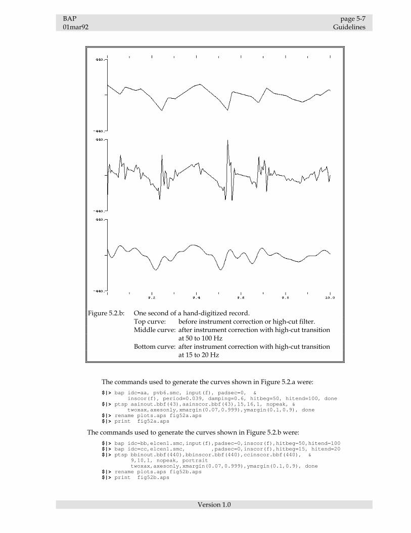
BAP page 5-7 01mar92 Guidelines
Version 1.0
The commands used to generate the curves shown in Figure 5.2.a were: $|> bap idc=aa, pvb6.smc, input(f), padsec=0, & inscor(f), period=0.039, damping=0.6, hitbeg=50, hitend=100, done $|> ptsp aainout.bbf(43),aainscor.bbf(43),15,16,1, nopeak, & twoxax,axesonly,xmargin(0.07,0.999),ymargin(0.1,0.9), done $|> rename plots.aps fig52a.aps $|> print fig52a.aps The commands used to generate the curves shown in Figure 5.2.b were: $|> bap idc=bb,elcen1.smc,input(f),padsec=0,inscor(f),hitbeg=50,hitend=100 $|> bap idc=cc,elcen1.smc, ,padsec=0,inscor(f),hitbeg=15, hitend=20 $|> ptsp bbinout.bbf(440),bbinscor.bbf(440),ccinscor.bbf(440), & 9,10,1, nopeak, portrait twoxax,axesonly,xmargin(0.07,0.999),ymargin(0.1,0.9), done $|> rename plots.aps fig52b.aps $|> print fig52b.aps
Figure 5.2.b: One second of a hand-digitized record. Top curve: before instrument correction or high-cut filter. Middle curve: after instrument correction with high-cut transition at 50 to 100 Hz Bottom curve: after instrument correction with high-cut transition at 15 to 20 Hz
Page 5-8 BAP Guidelines 01mar92
Version 1.0
(Software bug: each of the three BAP commands above include a padsec=0 statement. The padsec=0 is required only to arrange that the curves to be plotted will all have the same start time. The current version of ptsp (a.k.a. TSPLOT) isn't smart enough to synchronize a padded with an unpadded time series when plotting a frame that doesn't show the beginning of the curves.) The time series shown in Figures 5.2.a and 5.2.b are available on the Strong-Motion CD-ROM at \1983\122x42PV.P0f and \1940\139u37EL.C0a respectively; the files are also distributed with the BAP distribution files as \agram\testdata\pvb6.smc and elcen1.smc. 5.3 Pre-filter Pads Before applying the high-cut or low-cut filter, BAP pads the beginning and end of the time series with a sequence of zeros. The user must verify that the zero pads are of sufficient length by inspecting plots of the velocity and displacement curves calculated from the padded, filtered acceleration. After either filter is applied, the time series in the pad areas will no longer be zero, but will show small oscillations that diminish as the distance from the recorded samples increases. When these filter transients are included in the integration bounds in the AVD step, and when the pads are long enough, the resulting velocity and displacement curves will begin and end at zero. The plots in Figures 5.3.a and 5.3.b illustrate the effect of the low-cut filter on two time series having pads of various lengths. The first time series is simply a two-second zigzag (which is not representative of an earthquake wave and is full of high-frequency components); wave forms that result from filtering and integrating this time series are shown in Figure 5.3.a. The second time series is recorded data from the Anderson Dam, downstream, recording site during the 1989 Loma Prieta earthquake. Wave forms that result from processing this time series are shown in Figure 5.3.b. There are four plot frames on each page and four curves in each plot frame. The four plots in each frame show the input time series, the filtered time series, the velocity calculated as the first integral of the filtered time series, and the displacement calculated as the second integral of the filtered input time series. The upper-left plot frame on each page shows the curves that result when no filter is applied; the upper-right frame shows the curves that result when a filter without padding is applied; the lower-left frame shows the results when the pads are too short; and the lower-right frame shows the results when the pad lengths are adequate. Only the low-cut filter was applied in these examples, because the effects of an appropriately-placed high-cut filter would have no significance in plots shown at this scale. The filter applied to the 2-second zigzag was placed with corner=0.75 Hz so that most of the curve would be filtered away, leaving the peak value so small that the filter transients are visible when the entire curve is shown. The roll-off parameter, nroll, was set to 4 for the zigzag filter to exaggerate the filter transients. The filter applied to the Anderson Dam time series was placed with corner=0.1 Hz and nroll=1.

BAP page 5-9 01mar92 Guidelines
Version 1.0
Input time-series file =zigzag.smc. Filter corner=0.75, nroll=4. The four plots in each frame above show the input time series (zigzag.smc), the filtered time series (periods longer than 1.3 sec. removed), the velocity calculated as the first integral of the filtered time series, and the displacement calculated as the second integral of the filtered time series.
no filter, no pad
filter without pad
filter with insufficient (5-sec.) pads
filter with sufficient (8-sec.) pads
Figure 5.3.a

Page 5-10 BAP Guidelines 01mar92
Version 1.0
Input time-series file =andds1.bbf. Filter corner=0.1, nroll=1. The four plots in each frame above show the input time series (andds1.bbf), the filtered time series (periods longer than 10 sec. removed), the velocity calculated as the first integral of the filtered time series, and the displacement calculated as the second integral of the filtered time series.
no filter, no pad
filter without pad
filter with insufficient (5-sec.) pads
filter with sufficient (20-sec.) pads
Figure 5.3.b
BAP page 5-11 01mar92 Guidelines
Version 1.0
The time series shown in Figure 5.3.b is the same time series that is used as the second example in Appendix B. The commands used to generate the curves in the
lower right-hand frame of Figure 5.3.b were: $|> bap idc=a4,andds1.bbf, & INPUT(f), PAD,padsec=20, LOCUT(f),corner=0.1, AVD(f), DONE $|> ptsp a4inout.bbf,a4acc.bbf,a4vel.bbf,a4dis.bbf, -20,60,80, & twoyax,twoxax,nopeak,rotate,notlbl, done $|> print plots.aps All the plot frames in Figures 5.3.a and .b were generated with similar commands. The above BAP command does not request instrument correction or related steps because those procedures, which affect high frequencies, have no significance with respect to the length of the pads required for the low-cut filter. (Pad lengths required by the low-cut filter are very much larger than those required by the high-cut filter.) The corresponding BAP command that does include INTERPolation to a denser sampling rate than the default 200 sps, INSCOR (which includes HICUT), and DECIMation is: $|> bap idc=a4, andds1.bbf, & INPUT(f) INTERP, spsnew=600 ! << only for densely-digitized data PAD, padsec=20, ktaper=zcross INSCOR, period=0.037, damping=0.60, hitbeg=50, hitend=100 DECIM, ndense = 3 ! << only for densely-digitized data LOCUT(f), corner=0.1,nroll=1 AVD(f), DONE
5.4 Tapers When an input time series that does not begin and end with amplitudes very near zero is extended with leading and trailing zero pads, there will be spurious sharp offsets in the padded time series where the recorded samples meet the pad areas. Passing these offsets through the INSCOR processing step (which includes the HICUT filter) will result in spurious high-frequency spikes. The tapering function, which is applied in the PADding process and which is controlled by the ktaper and tapsec run parameters, is used to smooth a discontinuity between recorded samples and the pad area. Ktaper(1) and (2) may be set to "zcross", "on", or "off". (Ktaper(1) refers to the beginning of the time series, ktaper(2) refers to the end, and ktaper without a subscript refers to both ends.) When ktaper=zcross, as it does by default, the recorded samples that occur before the first zero-crossing and after the last zero crossing are reset to zero. When ktaper=on, the end sections of the unpadded time series, each tapsec seconds long, will be multiplied by a cosine half-bell taper with the zero element of the taper applied to the last point in the leading pad and the first point of the trailing pad. When ktaper=off, no attempt is made to minimize the offsets between the recorded samples and the zero pads. Figure 5.4.a illustrates the three ktaper options as applied to the end of the Anderson Dam time series (the same time series as is shown in Figure 5.3.b and in Appendix B). The top-most curve shows the last second of the time series before the trailing zeros were added; the next curve shows the same curve as above, but with trailing zeros; the next curve shows the padded time series with the default ktaper=zcross option in effect; and the lowest curve shows the padded time series with the ktaper=on option in effect (with tapsec=0.2). Figure 5.4.b shows the resulting curves after the INSCOR+HICUT step has been applied to the padded, tapered curves in Figure 5.4.a. Note that the effect of a recorded-data-meeting-zero-pad offset is present in the top curve in Figure 5.4.b even though that
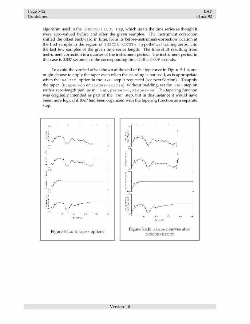
Page 5-12 BAP Guidelines 01mar92
Version 1.0
algorithm used in the INSCOR+HICUT step, which treats the time series as though it were zero-valued before and after the given samples. The instrument correction shifted the offset backward in time, from its before-instrument-correction location at the first sample in the region of INSCOR+HICUT's hypothetical trailing zeros, into the last few samples of the given time series length. The time shift resulting from instrument correction is a quarter of the instrument period. The instrument period in this case is 0.037 seconds, so the corresponding time shift is 0.009 seconds. To avoid the vertical offset shown at the end of the top curve in Figure 5.4.b, one might choose to apply the taper even when the PADding is not used, as is appropriate when the velfit option in the AVD step is requested (see next Section). To apply the taper (ktaper=on or ktaper=zcross) without padding, set the PAD step on with a zero-length pad, as in: PAD,padsec=0,ktaper=on. The tapering function was originally intended as part of the PAD step, but in this instance it would have been more logical if BAP had been organized with the tapering function as a separate step.
Figure 5.4.a: ktaper options
Figure 5.4.b: ktaper curves after
INSCOR+HICUT

BAP page 5-13 01mar92 Guidelines
Version 1.0
5.5 Velocity and Displacement As illustrated in the plots in Figures 5.3.a and 5.3.b, the velocity and displacement time series integrated from a low-cut filtered acceleration time series will begin and end at zero when sufficient pad lengths are used. The final ground displacement cannot be obtained from a filtered record, only from a record that has been digitized so accurately that filtering is not required, and then only if the initial velocity is known. The integrations performed in BAP use zero as the initial value for velocity and displacement. Initial values of zero are appropriate for records made by digital recorders that have a pre-event memory and provide in their records several seconds of motion that occurred before triggering of the recording device. Initial values of zero are also used for digitized analog records, for lack of more appropriate values, but the actual initial values are unknown and non-zero because these records start only after the earthquake motion has become strong enough to trigger the recorder, not with the very beginning of the earthquake. Although the unknown initial velocity and displacement for triggered records should be very close to zero if the recorder triggered early in the earthquake, even a small unknown initial velocity will have a large influence on the shape of the displacement curve calculated from the velocity curve. The velfit option in the AVD step can be used to obtain estimates of the initial acceleration and velocity for those triggered analog records that were recorded and digitized so accurately that the low-cut filter is not required. After the acceleration is integrated to velocity, a sloped, fitted line is subtracted from the velocity and a constant, equal to the slope of the line, is subtracted from the acceleration. The velocity is integrated to displacement after the line has been subtracted. The subtracted line is the linear least-squares fit to a user-specified portion of the velocity. On the assumption that the velocity must be zero after the earthquake, the fit should be applied to the final portion of the velocity, where the strong motion has subsided. Although the correcting line may be determined from just a section of the velocity, the extrapolated line is subtracted from the entire velocity time series. Velfit is a rarely-used option that should only be applied to accurately recorded, accurately digitized records for which no LOCUT filter is required. Note that velfit=on requires that LOCUT=off (which is equivalent to NOlocut), padsec=0.0 (that is, no padding), and that the input is acceleration, not velocity. 5.6 Low-Cut Filter Corners The LOCUT processing step removes low-frequency noise from a time series with a bidirectional Butterworth filter. The user must select transition parameters for the filter (corner and nroll) that allow as much as possible of the low-frequency content of the signal to pass though the filter yet remove that part of the signal that is overly contaminated by noise. These are conflicting requirements that vary from station to station, possibly even from trace to trace on the same record. It is always desirable to retain periods as long as, or longer by a factor of two than, the rupture duration of the earthquake, insofar as this can be approximated by the strong-motion duration of the record3. In structural records, it is of course desirable to retain
3 Reference [3], by Basili and Brady (1978).
Page 5-14 BAP Guidelines 01mar92
Version 1.0
content at periods equal to or greater than the longest natural period of the fundamental resonant modes of the structure. Several opportunities exist for determining the frequency below which (or periods above which) noise problems are present. 1) The corrected, filtered acceleration, after two integrations, should yield a
displacement time series that contains long periods consistent with those expected by seismological theory and experience and with records from traditional displacement meters.
2) Long-period content in displacement curves derived from stations sufficiently
close to each other should be coherent. That is, they will have similar shapes, although offset by applicable small time intervals. See, for example, References [9], by Hanks and Brady, and [10], by Hanks.
3) Displacements from recorders within the same structure should be coherent at
periods longer than the natural periods of the fundamental resonant modes of the structure.
4) The Fourier amplitude spectrum and the pseudo-velocity response spectrum of a
noise-free record should fall off more or less smoothly at low frequencies except for resonances in structures or in soft ground. Any other behavior is suggestive of noise, particularly if concentrated within a specific frequency range. Possibilities for the introduction of noise at a specific low frequency include photographic distortion, digitizing table distortions, and other mechanical sources.
5) The Fourier amplitude spectrum of a reference trace, digitized in the normal
course of digitization of all traces on a record, is a basic measure of noise in the recording system and digitizing system at all frequencies. During routine processing some low-frequency noise sources, resident in the recorder itself, are removed from the signal during the subtraction of the reference trace, followed by subtraction of the mean value (processing steps that are performed by the AGRAM/SCALE program at the USGS). If these recorder-resident noise sources are insignificant, the reference traces are close to truly straight. In that case, the reference trace spectral level represents only digitization noise, which is probably dominant at those periods where the reference trace spectral level is as large as the spectral level of a digitized accelerogram.
6) One need not require that the recorder-resident noise sources are insignificant, in
item # 5 above, if a truly straight line is available. The Fourier amplitude spectrum of a true straight line, digitized as though it were an acceleration trace, provides an indication of noise in the digitizing system (independent of the recording system) at all frequencies. Digitization noise is probably dominant at those periods where the spectral level of a digitized straight line is as large as the spectral level of a digitized accelerogram. A true straight line can be produced on a dimensionally stable film (held planar) by exposing the film to all but the shadow of a piece of copper wire pulled in tension past its yield point. The shadow must be cast by a point light source to obtain a sharp-edged line and the wire should be approximately parallel to the film to obtain a shadow of uniform thickness.

BAP page 5-15 01mar92 Guidelines
Version 1.0
7) The time series files in the Strong-Motion CD-ROM often contain suggested filter parameters. When processing such a file, BAP will use the suggested parameters from the file if the user has not provided an explicit value for the corner run parameter. Many files in the CD-ROM contain "undefined" suggested filter parameters, however. In such cases the user must consult the references indicated in the comments section of the file or use one of the above techniques to determine an appropriate low-cut filter corner.
5.7 Filter Transitions Filters having broad transitions between their pass-band and stop-band, like the BAP HICUT filter with its default transition band at 50 to 100 Hz (for LSA-digitized records) and the LOCUT filter with its default nroll=1, are preferable to filters having narrow transition bands. Filters with narrow transitions produce oscillations at frequencies near the cut-off frequencies, as shown in Reference [8], by Fletcher and others. The filter applied in the zigzag examples in section 5.3 used nroll=4, just to show exaggerated filter transients. If nroll=1 is used instead, the oscillations are reduced and the pad length can be reduced from 8 to 3 seconds, as is shown in Figure 5.7.
Figure 5.7
Page 5-16 BAP Guidelines 01mar92
Version 1.0
5.8 Fourier Amplitude Spectra The fast Fourier transform, or FFT, used in the FAS processing step to transform a time series to the frequency domain requires that the number of samples in the time series be an integral power of 2. BAP will add trailing zeros before applying the FFT if the number of leading and trailing zeros plus the number of samples in the input time series is not an integral power of 2. The trailing zeros that are appended for the FAS process are, in the default case, simply appended to the end of the current time series with no tapering, under the assumption that the time series has already been tapered to the pad in the earlier PAD step. When the PAD step is not applied in preparation for the HICUT or LOCUT filter, however, the user should usually set the jpad run parameter to request that the trailing zeros be added not in the FAS step, but in the PAD step so the ktaper=zcross or ktaper=on tapering function that is part of the PAD step can be performed. The jpad run parameter controls the padding sequence. By default, when jpad=5, short 2-second pads are added before the INSCOR+HICUT step, the pads are then extended (to tapsec seconds) before the LOCUT step, then the trailing pad is extended again (to 2n samples) in the FAS step. When one is using BAP to plot the Fourier amplitude spectrum of an unfiltered time series, it is best to set jpad=0 so the trailing zeros required for the FAS step are appended in the PAD step, along with the default ktaper=zcross tapering. For example, a plot of the Fourier amplitude spectrum of the input time series used for the first example in Appendix B can be generated with the following two commands: $|> bap idc=xx, gilroy21.smc, jpad=0, FAS(p) $|> print xxplots.aps (This assumes that the gilroy21.smc data file has been copied to the user's local directory.) See Chapter 3 for more information about jpad, Section 5.4 of this Chapter for more information about the tapering. To compare Fourier amplitude spectra from several different time series, it may be advantageous to arrange that the sampling interval in the frequency domain be the same for each spectrum in the comparison, so the spectra can be compared point by point. The sampling interval in the frequency domain is the reciprocal of the time-series duration, the product of the sampling interval in the time domain and the number of time-domain samples. Consequently, the user may wish to pad the shorter of two time series (whose Fourier amplitude spectra will be compared) with enough trailing zeros that the lengths of the two padded time series are equal. The user can indicate the size of the trailing pad required through the padsec(2) run parameter. Note that spectral plots from the FAS step show increasing frequency from left to right along the horizontal axis (see Figures 5.6.a and .b for example), in contrast to the plots from the RESPON step, which show increasing period (see Figure 5.9 for example). Note also that FAS plots of a filtered time series, such as the one in Figure B.3.d in the Examples Appendix, will often show dense fluctuations at very low amplitude and at frequencies that are higher than the transition band of the HICUT filter. These fluctuations are at the limit of the accuracy of the computer's floating-point numbers, relative to the peak value in the Fourier spectrum, and have no significance other than to indicate that the Fourier content has been removed at those frequencies.

BAP page 5-17 01mar92 Guidelines
Version 1.0
5.9 Response Spectra The range of the spectrum presented by the RESPON step is restricted to periods equal to or greater than ten times the sampling interval of the time series, 10∆t, due to limitations in the algorithm used by BAP for calculating maximum-response values. This limitation is mentioned on pages 914-915 of Reference [16], by Nigam and Jennings. The paper discusses the limitation of the algorithm in terms of the interval of integration, which in the BAP application of the algorithm is the same as the sampling interval of the time series. For time series sampled at 200 samples per second, like those from the Strong-Motion CD-ROM, the lowest period in the response spectrum should be at or above 0.05 seconds, which is the default value for the beginning of the spectrum, sper(1). Even if the user specifies a lower value for sper(1), the RESPON curves will not extend below 10∆t except in special cases where the cliprs run parameter is set to off. By default, cliprs=on; the cliprs=off setting is meant only for use in test situations where one wishes to investigate the behavior of the response spectra calculations below the critical period of 10∆t. A user who requires response spectra with periods that extend below 10∆t could reinterpolate the input time series to a denser sampling rate before applying the RESPON step. The response spectra algorithm would be stable down to the new value for 10∆t, but the user would need to keep in mind that there is no real frequency content in the more densely-sampled version of the time series above the Nyquist frequency (having a period of 2∆t) of the original sampling. This must be taken into account when making use of response spectra calculated from some of the time series on the CD-ROM also. Although most of the time series in the CD-ROM collection are given at 200 samples per second, some of the older records were originally digitized at much coarser sampling rates. For instance, the El Centro record used in the example in Figure 5.2.b was originally digitized at an average of only 18 samples per second, but it is given on the CD-ROM at 200 samples per second. A sample plot from the RESPON step is shown in Figure 5.9. The five curves represent the five damping fractions given for sdamp. (In this case, sdamp = 0.0, 0.02, 0.05, 0.1, and 0.2, which are the default values.) The number of dots in the dash-dot pattern of the curves indicate increasing damping fraction: the solid line is the curve corresponding to sdamp(1), the line with a single dot in its pattern corresponds to sdamp(2), and so forth. The vertical line at 0.05 seconds serves as a warning that the response curves extending to the left of that line are inaccurate. The plot was generated with cliprs=off. If cliprs had been set to on (the default), the curves would not have extended below 0.05 seconds, even though a lower spectral range was requested via sper(1). The plot was generated with the following commands: $|> bap idc=xx, mydata.bbf, respon(p), cliprs=off & sdamp= 0.0, 0.02, 0.05, 0.100, 0.20 sper= 0.04, 0.05, 0.1, 0.2, 0.5, 1.0, 2.0, 5.0, 10.0, 15.0 sdper= 0.002, 0.005, 0.01, 0.02, 0.05, 0.1, 0.2, 0.5, 1.0, done $|> print xxplots.aps

Page 5-18 BAP Guidelines 01mar92
Version 1.0
5.10 Some Sample Command lines The input commands and corresponding results from two sample BAP runs that illustrate complete processing for two different time series are presented in Appendix B. A few more sample commands are shown in this section to illustrate various other ways of using BAP. These examples are shown as though they were invoked on a PC computer, but that is only because they make use of the PC versions of default BAP output file names rather than the VAX versions. The default BAP output file names all begin with the three characters "bap" on a VAX, while they begin with the two characters "bp" on a PC (because PC filenames are limited in length). The examples in this section, like all the examples in this report, make use of a print command that communicates with a PostScript printer. The printing function may require a different command on some computers. To use BAP merely to generate a screen plot of a time series from the Strong-Motion CD-ROM, one could use: dos> bap tsdata.smc dos> scrplot bpplots.aps In this example, the file named tsdata.smc (which could be a copy of any of the time series data files from the Strong-Motion CD-ROM) is given as the only parameter on a BAP command line. By default, when no processing steps are requested, BAP generates a plot of its input file, placing the plot information in a file
Figure 5.9

BAP page 5-19 01mar92 Guidelines
Version 1.0
named bpplots.aps (bapplots.aps on a VAX). The SCRPLOT program, as shown above, can then be used to display the plot on the user's screen. Or, for a hard-copy plot, the bpplots.aps file could be sent to a PostScript printer: dos> print bpplots.aps. To convert a SMC-format data file to BBF format, so one could plot the time series using options provided by the TSPLOT program, one could use: dos> bap tsdata.smc, input(f), outfmt=bbf dos> rename bpinout.bbf tsdata.bbf dos> stsp tsdata.bbf, 10.2,10.4,0.2, pltdots In this example, BAP's reformatted output file, initially named bpinout.bbf then renamed to tsdata.bbf, is plotted via the STSP program, the screen version of TSPLOT. Only the interval from 10.2 through 10.4 seconds is plotted and, due to the pltdots requested on the STSP command line, each plotted sample is marked with a small dot. To convert the other way, from a BBF-format file to a SMC-format file, one could use: dos> bap mydata.bbf, input(f), outfmt=smc dos> rename bpinout.smc mydata.smc Note that one can convert a SMC-format file to a BBF-format file and back again to a SMC-format file without losing any of the auxiliary header information. Some header information may be lost, however, if one converts a BBF-format file to a SMC-format file and back again to a BBF-format file. Any leading or trailing pad samples in the original BBF-format file would also be lost if one converted a BBF-format file to a SMC-format file and back again to BBF-format, for BBF files include the pad samples and SMC-format files do not. 5.11 Run Messages Diagnostic messages written by BAP show three asterisks (***) in the left-hand margin of the screen display and in the left-hand margin of the bprun.msg (baprun.msg on a VAX) file. By default, the program will stop after printing such a message, but whenever users reset the default warn=stop to warn=bells or warn=msg, it is important that they check the run messages for "***" diagnostics before trusting the validity of BAP's plots or output data files.

Page 5-20 BAP Guidelines 01mar92
Version 1.0

BAP page 6-1 01mar92 Support Programs
Version 1.0
Chapter 6
Support Programs Miscellaneous support programs that can be used in conjunction with BAP are listed in this Chapter. Many of these support programs are not available for PCs yet, but PC versions may be added in the future. Instructions for using each program are displayed on the user's computer screen when the name of the program, with no command line arguments added, is typed in response to the prompt from the operating system. More information about each program is available through the HELP command, and more information about the plotting programs is available in Chapter 7. VAX PC Program Program ? ? name function n.a. yes LOWBAP An alternative version of BAP for PCs that loads faster
than PC/BAP does. LOWBAP executes more slowly than BAP and it will truncate a long time series, but it can be more convenient than BAP in some cases: when one is simply using BAP/LOWBAP to reformat a short time series file, for instance, and does not require that BAP/LOWBAP do many computations. BAP is a 32-bit protected-mode program that runs in extended memory; LOWBAP is a 16-bit real-mode version of the same program that runs in conventional (or "low") memory. LOWBAP limits (truncates) the time series it can deal with to 16K samples; that's 80 seconds of an evenly-sampled, 200-sample-per-second time series.
yes1 yes SCRPLOT Screen plotting program. SCRPLOT will display the
contents of an AGRAM-PostScript file (a .aps file) on the user's screen. On the USGS VAXes, SCRPLOT will also display the contents of a batch.plt file (or any binary plot file generated by the USGS VIEWER/PLOTLIB software). SCRPLOT can only interpret the limited
1 Some programs indicated as being available on VAXes are available only on the
USGS VAXes in Menlo Park; they are not included with the BAP distribution files.

BAP page 6-2 01mar92 Support Programs
Version 1.0
VAX PC Program Program ? ? name function PostScript conventions used in AGRAM-PostScript files, it
is not a general-purpose PostScript interpreter. TSPLOT Time-series plotting program for blocked-binary time-
series data files (.bbf files). TSPLOT offers far more flexible plotting options than does BAP. See Chapter 7 for more information.
yes yes PTSP PostScript-plotting version of TSPLOT. yes1 yes STSP Screen-plotting version of TSPLOT. FASPLOT Fourier amplitude spectra plotting program for blocked-
binary time-series data files (.bbf files). FASPLOT offers far more options for Fourier amplitude spectra plots than does BAP. See Chapter 7 for more information.
yes yes PFAS PostScript-plotting version of FASPLOT. yes1 yes SFAS Screen-plotting version of FASPLOT. SMCPLOT Time series plotting "program" for SMC-format time-series
data files (.smc files). This is implemented with .bat files that invoke BAP to reformat the SMC-format file to a BBF-format file then invoke TSPLOT to plot the contents of the new file. The main purpose for this "program" is to provide the psmc.bat and ssmc.bat files as examples of how to use TSPLOT with SMC-format data files.
yes yes PSMC PostScript-plotting version of SMCPLOT. yes1 yes SSMC Screen-plotting version of SMCPLOT. no no RSPLOT Response spectra plotting program. This program isn't
available yet, but should be added to the AGRAM programs to provide more options for response spectra plots than are available in BAP.
yes1 yes TXTMODE Resets the video from graphics mode to text mode. Use
this after a screen-plotting program aborts (or you abort one intentionally with Control+C), leaving the screen in graphics mode. For more information, see step 2 of Section E.3 in the Installation Appendix.
n.a. yes MSHERC Video support software for Hercules-compatible monitors
and adaptors on PCs. For more information, see step 6 of Section E.2 in the Installation Appendix. This software was provided by Microsoft with their Fortran compiler.
n.a. yes WHATMEM Indicates whether and how much extended memory is
available on the computer. This software was provided with the Ergo OS386 DOS-extending software used by PC/BAP. For more information see step 8 of Section E.2 in the Installation Appendix.
no yes ASC2PS Text-to-PostScript converting program. This "shareware"
software was provided by B.W.Miller. n.a. yes WMBOOT Warm-Boot command for PCs. See
c:\agram\docs\altboots.doc for more information. yes no BBFDMP Blocked-binary data-file dumping program.
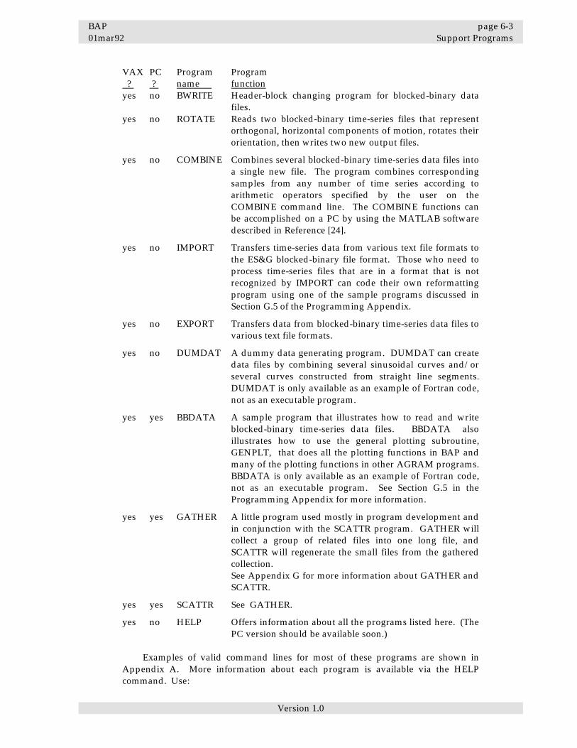
BAP page 6-3 01mar92 Support Programs
Version 1.0
VAX PC Program Program ? ? name function yes no BWRITE Header-block changing program for blocked-binary data
files. yes no ROTATE Reads two blocked-binary time-series files that represent
orthogonal, horizontal components of motion, rotates their orientation, then writes two new output files.
yes no COMBINE Combines several blocked-binary time-series data files into
a single new file. The program combines corresponding samples from any number of time series according to arithmetic operators specified by the user on the COMBINE command line. The COMBINE functions can be accomplished on a PC by using the MATLAB software described in Reference [24].
yes no IMPORT Transfers time-series data from various text file formats to
the ES&G blocked-binary file format. Those who need to process time-series files that are in a format that is not recognized by IMPORT can code their own reformatting program using one of the sample programs discussed in Section G.5 of the Programming Appendix.
yes no EXPORT Transfers data from blocked-binary time-series data files to
various text file formats. yes no DUMDAT A dummy data generating program. DUMDAT can create
data files by combining several sinusoidal curves and/or several curves constructed from straight line segments. DUMDAT is only available as an example of Fortran code, not as an executable program.
yes yes BBDATA A sample program that illustrates how to read and write
blocked-binary time-series data files. BBDATA also illustrates how to use the general plotting subroutine, GENPLT, that does all the plotting functions in BAP and many of the plotting functions in other AGRAM programs. BBDATA is only available as an example of Fortran code, not as an executable program. See Section G.5 in the Programming Appendix for more information.
yes yes GATHER A little program used mostly in program development and
in conjunction with the SCATTR program. GATHER will collect a group of related files into one long file, and SCATTR will regenerate the small files from the gathered collection.
See Appendix G for more information about GATHER and SCATTR.
yes yes SCATTR See GATHER. yes no HELP Offers information about all the programs listed here. (The
PC version should be available soon.) Examples of valid command lines for most of these programs are shown in Appendix A. More information about each program is available via the HELP command. Use:

BAP page 6-4 01mar92 Support Programs
Version 1.0
$|> help program-name $|> help agram-topics $|> help topic
BAP page 7-1 01mar92 Plots
Version 1.0
Chapter 7
Plots BAP provides plots by writing plot descriptions in the PostScript language1 to a disk file named bapplots.aps (or something similar). The bapplots.aps file can be sent directly to a PostScript printer with the print command (i.e., $|> print bapplots.aps) or viewed on the user's screen via the SCRPLOT program included among the BAP support programs (i.e., $|> scrplot bapplots.aps). If the user's printer is not a PostScript printer, the bapplots.aps file must be translated from PostScript format into a format the printer can accept. There are several commercially available PostScript-to-other-printer-format conversion programs that can be used to do the translating. The \agram\docs\comsoft.nts file included among the BAP distribution files lists the names and addresses of several software companies that provide PostScript-to-other-printer translating software for PCs. 7.1 Plotting Programs The plotting support programs distributed with BAP are TSPLOT, FASPLOT, and SCRPLOT. TSPLOT generates time-series plots, FASPLOT generates Fourier amplitude spectra plots, and SCRPLOT displays the plot(s) described in an AGRAM-PostScript file on the user's screen. The BAP program will also generate time-series plots and Fourier amplitude spectra plots, but TSPLOT and FASPLOT offer the user more control over the appearance of the plots than does BAP. There are two versions of TSPLOT and FASPLOT (and more than two versions of each on the USGS VAXes -- see section 7.6). Each version of TSPLOT and FASPLOT is distinguished from the other version of the same program by the first character of the version name, with that first character indicating the plotting medium. The two versions of TSPLOT are stsp and ptsp: stsp plots on the user's screen and ptsp writes a plot description to a PostScript file. The two versions of FASPLOT are sfas and pfas. TSPLOT and FASPLOT require blocked-binary time-series data files as input files; SCRPLOT requires an AGRAM-PostScript file as its input file. The blocked- 1 The PostScript page description language is described in References [1] and [2].

page 7-2 BAP Plots 01mar92
Version 1.0
binary time-series data files (.bbf files) are generated by the BAP program; the AGRAM-PostScript plot-description files (.aps files) are generated by BAP, PTSP, and PFAS. The contents of an AGRAM-PostScript file can be sent to a PostScript printer for hard-copy plots or processed through SCRPLOT for screen plots. Examples: $|> scrplot plots.aps $|> print plots.aps (only if the print command is
connected to a PostScript printer!) To use TSPLOT, FASPLOT, or SCRPLOT, the user can simply type the name of the program followed by the name of the program's input file. Examples: $|> stsp mytsdata.bbf $|> pfas bapvel.bbf $|> scrplot bapplots.aps Many additional options are available in TSPLOT and FASPLOT, however.
7.2 Screen Plots If one of the screen-plotting programs (SCRPLOT, STSP, SFAS) aborts, the user will need to reset the video mode from graphics mode back to text mode. Use the TXTMODE command to do so: $|> txtmode The characters shown in the PC screen plots may be so small that you can barely read them, especially if you have a small screen. If you really need to read the characters, you can request that the screen-plotting programs use normal PC display characters rather than the tiny plotted characters that are used by default. Set the "msfonts" environment variable to indicate which type of characters should be displayed. When msfonts=no, the normal PC display characters are used, when msfonts is undefined or set to a directory that contains a modern.fon file, the characters are drawn according to the information given in the modern.fon file. (By default, the PC screen-plotting programs attempt to find the modern.fon file in the c:\agram\exes directory.) For more information about msfonts and PC screen plots, refer to step 2 in Section E.3 of the Installation Appendix.
7.3 Plotting on Computers other than PCs The PC versions of the BAP support programs that plot on the user's screen (SCRPLOT, STSP, and SFAS) use calls to subroutines provided by the Microsoft PC fortran compiler to make the plots. User's wanting to install the screen-plotting support programs on computers other than PCs will need to provide a software interface between the distributed code and whatever screen plotting software is available on the relevant computer. This is true for VAXes as well, for the screen-plotting software used with BAP on the USGS VAXes in Menlo Park is not included with the BAP distribution files. Or, rather than modify the screen-plotting BAP support programs, users could use one of the commercial software packages that display PostScript plots on computer screens. On some other-than-PC computers, users may want to modify the plotting software that generates hard-copy plots in addition to modifying the screen-plotting
BAP page 7-3 01mar92 Plots
Version 1.0
software. The AGRAM-PostScript processing is rather slow, so it may be preferable to change the programs to use whatever intrinsic plotting software is available on the relevant computer rather than to use the PostScript-plotting versions distributed with BAP. See Appendix G for more information about the BAP/AGRAM source code. Section G.4 discusses the plot interface. 7.4 TSPLOT, Time-Series Plotting program TSPLOT plots the contents of the blocked-binary time-series data files produced by BAP and other AGRAM programs. Refer to the figures in Chapter 5 for examples of TSPLOT output plots. To run TSPLOT in its simplest form, type the name of the version you wish (stsp or ptsp), followed by the name of one or more blocked-binary time-series data files, as in: $|> stsp mydata.bbf, yourdata.bbf Or, to override the default parameters, use -- stsp bbf-input-file(p), bbf-input-file(#) bbf-input-file(#,#), ... (any number of bbf file names) ... title-file, tbegin,tend,spp,ysize,yspace, flags where flags are any combination of: nopad, dots, portrait,
nosync, nocc, arrow, circle, nopeak, nolabels, axesonly, noxlbl,noylbl, notlbl, noxax, onexax, twoxax, oldxax, noyax, oneyax, twoyax, seb, xmargin(#,#), ymargin(#,#), upcase, runmsg(filename)
The bbf-input-file names specify disk files containing the time series to be plotted. When the names of several files to be listed on a TSPLOT command line have the same prefix and only differ in their suffixes, the prefix need only be given in the first name listed. The name of a text file that contains a top-of-plot title may also be included. Example: $|> stsp mydata.a01,.a03, yourdata.a01,.a03, topplot.txt This example uses default scaling and labeling options. Each resulting plot page shows 20 seconds of each time series curve (one curve for each blocked-binary time-series file given on the command line). The curves are shown in separate strips across the page, each strip with its own y-axis, and the width of the strips (length of the y-axes) depending on the number of curves on the page. The first two significant digits, plus one, of the peak value of a curve are used for the scale on that curve's y-axis. The title at the top of the plot will come from the text file specified in the command line, or if there was no text file, the title will consist of the names of the time-series files. To alter the vertical scale for any curve, the user may include one or two numbers, or a "p", in parentheses after the file name to indicate the range for the y-axis. If two numbers are given, they indicate the minimum and maximum value for

page 7-4 BAP Plots 01mar92
Version 1.0
the axis; if just one number, it indicates the maximum value for the axis and the absolute value of the axis minimum. If there is a "p" in the parentheses, the peak value found in the curve will be used as the y-axis limit, without any rounding adjustment to the value. Example: $|> stsp mydata.r01(p),.r02(-15,+25),.r03(30) To alter the size of the y-axes and the range of the x-axis, one may include up to five numeric parameters after the file names on the command line. The meaning of these numbers depends on the order in which they are given, so give a null value (two consecutive commas) if you wish to use a default value among other parameters you wish to set. The numeric parameters and the order in which they must be given are: tbegin, tend, spp, ysize, yspace. tbegin is the time at which the plot will begin. Default = the time corresponding
to the time of first sample in the earliest time series to be plotted. tend is the time at which the plot will end. Default = ending time of the late-
most ending curve. spp are the number of seconds to appear across each plot page. Default =20.0.
If tend - tbegin is greater than spp, more than one page will be plotted.
ysize is the size of the y-axes, given as a fraction of the plot page. yspace is the size of the space to be left between the plot strips, given as a fraction
of the plot page. To compare the shapes of curves plotted in several different TSPLOT runs, it is often a good idea to provide a value for ysize so that all the curves to be compared use a y-axis of the same size. If ysize is not specified, TSPLOT will choose a value that depends on the number of lines in the top-of-plot title and on the number of curves to be plotted on the page. Ysize values of 0.7, 0.3, 0.2, and 0.14 work well for one, two, three, and four curves per plot page, respectively. When ysize is small enough, and the time axis is longer than will fit across one page, the plot will be continued on the same page as the first plot rather than on another page. Example: vax$ stsp pub1:[agram.testdata]eda.a01,0,15,5, 0.18 In addition to the five numeric parameters that control how the plots will appear, there are a number of keywords that may be included on the command line (in any order) to affect the appearance of the plots. The recognized keywords are: nopad, dots, portrait, nosync, nocc, arrow, circle, nopeak, nolabels, axesonly, noxlbl,noylbl, notlbl, noxax, onexax, twoxax, oldxax, noyax, oneyax, twoyax, seb, xmargin(#,#), ymargin(#,#), upcase, and runmsg(filename). nopad By default, TSPLOT will show the leading and trailing pad areas that
may have been added to the beginning and end of the time series by the BAP program (or the older CORAVD, AVD, or ADDPAD programs). To override this default and request that the pads not be shown, include "nopad" on the command line.
dots Include "dots" on the TSPLOT command line if you wish to have
each plotted point marked with a little circle. dots should not be requested unless a very small segment of the time series is to be
BAP page 7-5 01mar92 Plots
Version 1.0
plotted, otherwise the plot will show many overlapping little circles. Example:
$|> stsp bapdis.bbf, 5.4,5.8,0.2,dots portrait The portrait flag is used to request that the plot page be rotated
from the default landscape orientation to portrait orientation. By default, the horizontal x axis is oriented across the wider dimension of the plot page, as in a landscape picture and as it makes sense to have the plots displayed on VDT screens, which are usually wider than they are high. But if "portrait" is included on the command line, the x-axis will be oriented across the narrower dimension of the plot page, as in a portrait picture. An example:
vax$ ptsp pub1:[agram.testdata]hz2and16.syn, & dummydata.syn, 4.dum,eda.a01, 30.dum,2890810o4.bse,.bne, eda.v01,dummydata.syn,eda.d01, portrait, twoxax,twoyax,noylbl,notlbl, ymargin(-0.01,-0.97) nosync and nocc: By default, when plotting more than one time series on a single
page, TSPLOT will attempt to syncronize the several time series using timing information that may be located in the header blocks of the input files. To request that the syncronizing not be performed, so the first sample of each time series will be shown at the first point on the x-axis no matter what timing information is in the header blocks, include "nosync" on the command line. To request that the syncronization be performed without including the clock correction values from the header blocks, include "nocc" on the command line. (The clock correction values are inaccurate in some of the blocked-binary time-series files in the ES&G data collection at the USGS.)
arrow, circle, and nopeak: These three options alter the way the peak values
in each curve are labeled. By default, the numeric value of the peak is shown just above the peak. But if "arrow" is included on the command line, a little arrow pointing to the peak will be used instead of the numeric label. If "circle" is on the command line, a little circle will mark the peak. And if "nopeak" is on the command line, the peak will not be labeled at all.
nolabels, axesonly, noxlbl, noylbl, notlbl and seb: These options
alter the other labels. With "nolabels" on the command line, no labels will be plotted, except perhaps those next to the peaks. "axesonly" is like nolabels except that the axes are plotted along with the curves. "noxlbl" omits the x-axis label, "noylbl" omits the y-axis label, and "notlbl" omits the top-of-plot label. Including noxlbl, noylbl, and notlbl on the same command line has the same effect as axesonly. The "seb" flag is used by members of the USGS to arrange the top-of-plot titles in a form suited for some of the data reports published by the USGS.
noxax, onexax, twoxax, oldxax, noyax, oneyax, and twoyax: These
options indicate how many x or y axes should be plotted. With
page 7-6 BAP Plots 01mar92
Version 1.0
twoyax, two y-axes are shown for each curve (left edge and right edge). With twoxax two x-axes are shown on each page (top and bottom), regardless of the number of curves on the page. Oneyax and twoxax are the current defaults.
xmargin(#,#) and ymargin(#,#): The xmargin and ymargin options allow
the user to define the size of the margins around the plots. The two numbers in parentheses following xmargin indicate the location of the left-hand and right-hand margins as fractions of the plot page; the two numbers in parentheses following ymargin indicate the location of the lower and upper margins, again as fractions of the plot page. If the numbers are positive, the various labels will be placed in the margins so that the x and y axes will fill the space between the margins completely. If the numbers in the parentheses are negative, the margins will be left empty, the labels will be placed in the plot space, and the axes shortened accordingly. The current defaults are xmargin(+0.15, +0.95) and ymargin(-0.05, -0.9).
upcase Indicates that the plot labels should be shown in upper case
characters. runmsg(filename) indicates the name of an optional output file that will contain
run messages and diagnostics that would normally be displayed on the user's screen.
7.5 FASPLOT FASPLOT plots the Fourier amplitude spectrum of evenly-sampled time series contained in blocked-binary data files. The time series must be evenly-sampled. To use FASPLOT with AGRAM/SCALE output files, which contain uncorrected, unevenly-sampled data, one must first create a file of uncorrected but interpolated data (using BAP or AGRAM/HIFRIC). To run FASPLOT in its simplest form, type the name of the version you wish (sfas or pfas), followed by the name of a blocked-binary time-series data file, as in: $|> sfas mydata.bbf Or, to override the default processing parameters, use: sfas FASfile= bbf-input-file1, bbf-input-file2, tbeg, tend, options where options are any combination of: misc-options,
computing-options, plot-axis-options, plot-title-options, and tsplot-style-options
misc-options are tsplot, nonoise, or runmsg(filename)
computing-options are any combination of: nsamples(#), datataper(#), zcross, notaper, smooth, nosmooth, fas, fasi, fasi2, fasd, fasd2 or fps

BAP page 7-7 01mar92 Plots
Version 1.0
plot-axis-options = any combination of: loglog,
loglin, linlog and linlin. plot-title-options = any combination of: top,
nolabels, notitle, axesonly; or the name of a text file containing the plot title.
tsplot-style-options = any combination of: portrait, xmargin(#,#), ymargin(#,#), upcase.
Some examples: dos> sfas \vaxdata\eda.a01 dos> sfas fromFAS.txt =c:\vaxdata\eda.r01, & zcross,smooth, fas,fasi,linlin,loglin,loglog $|> sfas mydata.bbf, & fas, loglog(-3,-,-2,3), fasi, loglog(-3,-,-2,3) $|> sfas mydata.bbf, xmargin(0.3,0.9) Up to three input file names can be specified on the FASPLOT command line. The bbf-input-file names specify blocked-binary data files containing the time series for which Fourier amplitude spectra plots are requested. Just one time-series data file is usually requested on a FASPLOT command line, but two time-series data file names can be given, in which case, Fourier amplitude spectra plots will be generated for each of the two input time series and a plot showing the ratio of the two specta will also be generated. The name of an input text file containing a top-of-plot label can also be given on the command line. An example: $|> pfas mydata.bbf,yourdata.bbf,topplot.txt The name of an output file to receive the Fourier amplitude spectrum values can be specified on the command line also. If given, the output file name should be the first parameter given on the command line after the program name (sfas or pfas), and it should be separated from the input file names with an equal sign. This output file will be a formatted text file, not a blocked-binary file. Another example: $|> pfas fas.txt= mydata.bbf The list that follows describes other options that can be indicated on a FASPLOT command line. tbeg and tend are numeric values that indicate the times, in seconds, that bracket
the section of the input time series to be processed. By default, tbeg and tend are the times corresponding to the first and last points on the input file, respectively. The default tbeg and tend bracket the entire input time series, including the leading and trailing pads, if any.
misc-options are tsplot, nonoise, or runmsg(filename) where: tsplot is an optional keyword that indicates that a plot of the padded, tapered time
series should be shown above each spectrum plot. nonoise is another optional keyword that indicates that the spectra plots should
not show amplitudes at frequencies above the hitbeg transition frequency used with BAP's high-cut filter (if such has been applied to the input time-series) or below the corner frequency used with

page 7-8 BAP Plots 01mar92
Version 1.0
BAP's low-cut filter (if such has been applied to the input time-series).
runmsg(filename) indicates the name of an optional output file to receive the run messages and diagnostics that would normally be displayed on the user's screen. It is often useful to specify a runmsg file when using sfas, since run messages displayed on the screen can interfere with the plots and vice-versa.
computing-options are any combination of: nsamples(#), datataper(#), zcross, notaper, smooth, nosmooth, fas, fasi, fasi2, fasd, fasd2 or fps, where: nsamples(#) specifies the length of the padded or truncated time series to be
transformed by the FFT. The number in parentheses must be an integral power of 2. By default, FASPLOT will add trailing zeros to the input time series, if necessary, to bring the number of samples up to an integral power of two.
datataper, zcross and notaper indicate how the discontinuity (if any) between the input time series and the trailing zeros (if any) should be treated. The datataper keyword may be followed by a real number in parentheses. The number must be between 0.0 and 0.5 and specifies the length of the taper as a fraction of the input time series length. (Note that the taper length is given to FASPLOT as a fraction of the time series length, in contrast to the taper length in BAP, tapsec, which is given in seconds.) The zcross keyword indicates that time-series samples before the first zero crossing or after the last zero crossing should be reset to zero.
smooth and nosmooth are Fourier amplitude smoothing options. The smooth keyword may be followed by an integer number in parentheses. The number should be odd and it specifies the number of weights to use in the triangular smoothing function. Note that smooth(1) and nosmooth are equivalent and are the default. Note too that it is the squared amplitudes that are smoothed when smooth is specified, not the amplitudes themselves.
fas, fasi, fasi2, fasd, fasd2 and fps are keywords that indicate the type of curves to be plotted: Fourier amplitude spectrum of the input time series (fas), Fourier amplitude spectrum of the time series integrated with respect to time (fasi), integrated twice (fasi2), differentiated (fasd), differentiated twice (fasd2), or Fourier phase spectrum (fps).
The default computing options are zcross, nosmooth, fas and nsamples(n), where n is the nearest power of two greater than the number of samples given in the input file. The plot-axis-options may include any or all of the four keywords that indicate the type of axes to use in the spectra plots. The keywords are: loglog, loglin, linlog and linlin. They indicate whether the x and y axes should be plotted in logaritmic or linear scale. Note that it is only in linlin and linlog plots that the first point, that for zero frequency, will be plotted. The loglog and loglin plots omit the zero-frequency point. By default, the program will choose the range for each axis, but users may specify these too, if they wish. Each type-of-axis keyword may be followed with parentheses containing four numbers, the numbers separated from one another with

BAP page 7-9 01mar92 Plots
Version 1.0
commas or blanks. The numbers indicate the beginning value for the x-axis, ending value for the x-axis, beginning value for the y-axis and ending value for the y-axis, respectively. A dash (-) may be used in place of any of the four numbers to indicate that the program should choose an appropriate number. For linear axes, the number is the actual value to be used at one end of an axis. For log axes, the number is an exponent of ten to be used at one end of an axis. The user-specified axis ranges will be adjusted, if necessary, so that log axes will begin and end at integral powers of ten, and linear axes will begin and end at some convenient number close to the user-specified number. When requesting that several types of curves be plotted (more than one of the fas, fasi, fasi2 ... options) and also specifying different axis ranges for each type of plot, one must repeat the plot axis options after each type-of-curve option. To do so, follow each type-of-curve option with the axis options applicable to that curve. Example: fas, loglog(-3,-,-2,3), fasi, loglog(-3,-,-2,3) The default plot axis option is loglog(-,-,-,-). The plot-title-options are any combination of: top, fig, doc, nolabels, notitles or axesonly; or the name of a text file containing the plot title. The top keyword (the default) indicates that the plot title should be shown at the top of the plot page. The top-of-plot title will consist of the input file names or the text from the input text file. In addition, the value of the computing options will be shown. The fig and doc options are rarely used (and may be removed from the program one day): refer to the information displayed via $|> help fasplot for information about these two options. The nolabels and axesonly keywords act as they do for the TSPLOT program. With nolabels, nolabels or axes will be plotted, just the curve. axesonly is like nolabels except that the axes are plotted as well as the curves. With notitles, the axes will be plotted and labeled, but there will be no title at the top of the plot. Other tsplot-style-options that work in FASPLOT as they do in TSPLOT are: portrait, xmargin(#,#), ymargin(#,#), upcase. These keywords have the same effect in FASPLOT as they do in TSPLOT.
page 7-10 BAP Plots 01mar92
Version 1.0
7.6 Additional Plotting Functions Available only on the USGS
VAXes There are two versions of BAP on the USGS VAXes, BAP and VWRBAP. BAP produces its plots in a postscript file (bapplots.aps), while VWRBAP produces its plots in a batch.plt file via the VIEWER/PLOTLIB plotting software used on the USGS VAXes. There are more than two versions of TSPLOT and FASPLOT on the USGS VAXes. In addition to the same stsp, sfas, ptsp, and pfas commands that are available for PCs, there are: dtsp and dfas, which write binary plot description information in
VIEWER/PLOTLIB format to a disk file named batch.plt. Several AGRAM and VIEWER replotting programs (e.g., scrplot, lsrplot, and viewer) can subsequently process the batch.plt file.
ltsp and lfas, which plot to the laser printer. vtsp and vfas, which plot to the Versatec printer. ctsp and cfas, which plot to the CalComp plotter. ntsp and nfas, which do not plot at all, but display the labels that would have
been plotted if a different version of the programs were used. (These are sometimes useful in debug situations.)
itsp and ifas, which issue prompts from the device-independent VIEWER/PLOTLIB plotting software that the user must answer to indicate which plot medium to use.
tsplot and fasplot, which are synonyms for itsp and ifas. The versions of TSPLOT and FASPLOT on the USGS/ES&G VAXes allow the user to indicate which typeface should be used for plot labels. To do so, include one of the typeface names on the command line: simple, romcom, romdup, romsim, romtrp, or cyrcom. After running dtsp, dfas, itsp or ifas, the plots in the resulting batch.plt file can be displayed on the user's screen via the scrplot command and/or they can be sent to the laser printer via the lsrplot command. The scrplot and lsrplot commands can distinguish whether they are dealing with a binary VIEWER/PLOTLIB plot description file or with an AGRAM-PostScript file. If the user types either scrplot or lsrplot without adding the name of the file that contains the plot description, the contents of the most recent version of batch.plt in the user's local directory will be plotted. The various AGRAM plotting commands (e.g., stsp, dfas, scrplot) are not really separate programs on the USGS VAXes (as they are in the PC versions) but are merely VAX/VMS indirect command files set up to run the device-independent version of the program (itsp, or ifas) with predetermined answers to the VIEWER/PLOTLIB prompts and with the results sent to the appropriate plotting device. As a consequence, the commands are somewhat clumsy:
• They display a lot of unnecessary run messages. • When something goes wrong, they give rather confusing diagnostic messages.

BAP page 7-11 01mar92 Plots
Version 1.0
• All the parameters on a command line must be separated from one another with commas: spaces will not work as parameter separators as they do in all the other AGRAM commands.
• No more than 8 spaces can be given on any command line: anything beyond the ninth space will be ignored.
• A long command must be continued from one line to the next by adding a dash (-) to the end of each line to be continued, rather than by adding the ampersand (&) to the end of just the first line.
To bypass the indirect command file processing, one can use the itsp or ifas versions of the plotting programs and answer the plotting system's prompts. For more information about the way plotting is handled on the USGS/ES&G VAXes, use: vax$ help agram-plots

page 7-12 BAP Plots 01mar92
Version 1.0

BAP BAP 01mar92 01mar92
Version 1.0
APPENDIXES

BAP page A-1 01mar92 Quick Reference
Version 1.0
Appendix A
Quick Reference The examples below illustrate the required arrangement of run parameters on the BAP command line and on the command lines for most of the support programs. The last of each set of examples is a generic example that shows items the user may supply in underlined, slanted characters and items the user must supply in double-underlined, slanted characters. The must-supply items are not required when the user merely wants to see a short display of information about the program, however: in that case, just the name of the program should be given on the command line. Note that the order in which the BAP command line parameters are given, with a few exceptions, has no significance. Most of the other AGRAM programs require that the command line parameters be given in a fixed sequence. Note, too, that $|> represents the prompt from the PC/DOS or VAX/VMS operating system, while vax$ represents the prompt from the VAX/VMS operating system. A.1 HELP
$|> help$|> help tsplot$|> help hitbeg$|> help agram$|> help agram-topics$|> help topic
A.2 BAP (See Section 4.1)
$|> bap show$|> bap mydata.smc$|> bap @runparam.txt$|> bap mydata.smc, @smc.brp, locut, corner=0.12$|> bap infile=mydata.bbf, pad, inscor, hicut, &
locut, corner=0.13, fas, done$|> bap baplocut.bbf, rspec(f,p)$|> bap data-file-name, step-name(f,p), @file-name &
runparameter-name=runparameter-value Default BAP run parameter values:
!! Step names and their associated parameters:!

page A-2 BAP Quick Reference 01mar92
Version 1.0
INPUTinfile= noname.xxx, infmt= *, motion?= ???, motion= *convert= 1.00
nointerpspsin?= 200., spsin= *, spsnew= 200.
nolincorvline= 0.00, mllsqf= off, mmean= off, beglin= *endlin= *, begfit= *, endfit= *, tapfit= 0.00
nopadpadsec= *, ktaper= zcross, tapsec= 0.20, jpad= 5
noinscorperiod?= *, period= *, damping?= *, damping= *
nohicuthitbeg?= 15.0, hitbeg= *, hitend?= 20.0, hitend= *
nodecimndense= 1
nolocutcorner?= *, corner= *, nroll?= 1, nroll= *, locut2= off
noavdvelfit= off
nofasnsmooth= 1
noresponsdamp= 0.00, 0.020, 0.050, 0.100, 0.20sper= 0.050, 0.100, 0.20, 0.50, 1.00, 2.00, 5.00, 10.0,
15.0sdper= 0.0050, 0.0100, 0.020, 0.050, 0.100, 0.20, 0.50,
1.00cliprs= on
!! output parameters:!
outfmt= BBF, outdir= [], idc= BAP, warn= stop SHOW= ONrunlbl= *
!! End of run parameter list.!done
A.3 TSPLOT (See Section 7.4) There are several different versions of TSPLOT, each distinguished from the other versions by the first character of the program name, with that first character indicating the plotting medium. PC versions of TSPLOT are: stsp (screen version) and ptsp (postscript version). Additional versions available on the USGS VAXes are: dtsp (meta-plot version that writes plot descriptions to batch.plt files), ltsp (laser printer version), and itsp (device-independent version).
$|> stsp mydata.bbf$|> stsp mydata.r01(p),.r02(-15,+25),.r03(30)$|> stsp mydata.a01,.a02,.a03,topplot.ttl$|> stsp [agram.testdata]eda.a01,0,15,5, 0.18$|> stsp bbf-input-file(p), bbf-input-file(#)
bbf-input-file(#,#), ... (any number of bbf file names) ...
tbegin,tend,spp,ysize,yspace, flags
where flags are any combination of: nopad, nosync, nocc,rotate, dots, arrow, circle, nopeak,nolabels, axesonly, noxlbl,noylbl,notlbl, noxax, onexax, twoxax, oldxax,noyax, oneyax, twoyax, seb,xmargin(#,#), ymargin(#,#), upcase.
BAP page A-3 01mar92 Quick Reference
Version 1.0
A.4 FASPLOT (See Section 7.5) There are several different versions of FASPLOT just as there are several different versions of TSPLOT. Versions for PCs are: sfas, and pfas; additional versions on the USGS VAXes are: dfas, lfas, ifas.
$|> SFAS [agram.testdata]eda.a01$|> SFAS fromSFAS.txt =pub1:[agram.testdata]eda.r01, &
zcross,smooth, fas,fasi,linlin,loglin,loglog$|> SFAS mydata.bbf, &
fas, loglog(-3,-,-2,3), fasi, loglog(-3,-,-2,3)$|> SFAS mydata.bbf, xmargin(0.3,0.9)$|> SFAS bbf-input-file$|> SFAS FASfile= bbf-input-file1, bbf-input-file2,
tbeg, tend, options
where options are any combination of: misc-options,computing-options, plot-axis-options,plot-title-options, and tsplot-style-options
misc-options are tsplot or nonoisecomputing-options are any combination of:
nsamples(#), datataper(#), zcross,notaper, smooth, nosmooth, fas, fasi,fasi2, fasd, fasd2 or fps
plot-axis-options are any combination of: loglog,loglin, linlog and linlin.
plot-title-options are any combination of: top,nolabels, notitle or axesonly; or thename of a text file containing the plottitle.
tsplot-style-options are any combination of:rotate, xmargin(#,#), ymargin(#,#),upcase.
A.5 SCRPLOT (See Section 7.1)
$|> SCRPLOT bapplots.apsvax$ SCRPLOT batch.plt (on USGS VAXes only)vax$ SCRPLOT (on USGS VAXes only)$|> SCRPLOT plot-description-file
A.6 SCATTR (See Section G.1)
$|> SCATTR bap.vax$|> SCATTR pcbap.add$|> SCATTR output-TOC-file = gathered-input-file
A.7 GATHER (See Section G.1)
$|> GATHER bap.vax = bap.wrk$|> GATHER pcbap.add = pcbap.wrk$|> GATHER all.txt = toc.txt$|> GATHER gathered-output-file = input-TOC-file

page A-4 BAP Quick Reference 01mar92
Version 1.0
A.8 AGRAM Programs that have no PC Version yet: The programs listed in this Section are not available with early versions of the PC distribution diskettes, but they may become available with future updates. BBFDMP:
vax$ BBFILE mylist.tmp=PUB1:[agram.testdata]eda.r01, 1-4,20vax$ BBFILE mydata.bbfvax$ BBFILE text-file= bbf-input-file,block-list
ROTATE: vax$ ROTATE new1.bbf,90, new2.bbf,180 =old1.bbf, old2.bbfvax$ ROTATE out-bbf1,dir1,out-bbf2,dir2 =in-bbf1,in-bbf2
or vax$ ROTATE out-bbf1,out-bbf2=in-bbf1,in-bbf2,epilat,epilong
COMBINE:vax$ COMBINE sum.bbf =a.bbf, b.bbf +vax$ COMBINE ave.bbf =a.bbf, b.bbf + 2.0 /vax$ COMBINE diff.bbf=a.bbf, b.bbf - eolvax$ COMBINE constant.bbf = 3, 5 + 2 /vax$ COMBINE newfmt.bbf=[agram.testdata]eda.a01, 0.0 +
ddstylevax$ COMBINE output-bbf = post-fix-list, options
where options may be: nosync, nocc, agstyle, ag,ddstyle, dd, dd10, and eol.
EXPORT:vax$ EXPORT temp.txt= mydata.bbf,dumpvax$ EXPORT newfile.eds=temporary.r01, .r02, .r03, .a01,
.v01, .d01, a02,.v02,.d02,.a03,.v03,.d03,
.ttl, EDISvax$ EXPORT outfile=input-bbf-file(s),format
where format = edis, dump, or beck IMPORT:
vax$ IMPORT 4scale.bbf =[agram.testdata]elcdamain.but,BUTTERvax$ IMPORT new. =[agram.testdata]tap154.001,PHASE1vax$ IMPORT new. =[agram.testdata]gilroy2a.dat, PHASE1vax$ IMPORT new. =[agram.testdata]cdmgsampl.ph1, CDMGP1vax$ IMPORT new.r01,.r02,.r03,tmp.tmp= &
[agram.testdata.oldcards]bkyec7.ph1, BKYP1vax$ IMPORT new. =[agram.testdata]ineltstr.ph0, PHASE2vax$ IMPORT output-bbf-prefix.= input-text-file, type, skip0
where type =butter, bky-butter, phase1, bkyp1,cdmgp1, or phase2
and skip0 is an extra option that works only withtype=butter.

BAP page A-5 01mar92 Quick Reference
Version 1.0
IOMTAP:
vax$ IOMTAP output-binary-file-name = drive,#-#or vax$ IOMTAP output-binary-file-name = input-file-name IOMPLOT: There are several different versions of IOMPLOT, just as there are for FASPLOT and TSPLOT. Versions: simp, pimp, dimp, limp, iimp.
vax$ LIMP iomtap-output-binary-file BUTTER:
vax$ BUTTER (prompts for input) SCALE:
vax$ SCALE 4hifric.= frombutter.bbf,0.5,1.92,1.85,1.77vax$ SCALE output-bbf-prefix = butter-output-bbf,
time-tick-butter-file,time-between-ticks,sens1,sens2,sens3
HIFRIC:
vax$ HIFRIC 4coravd.g01 =fromscale.r01,.040,.570vax$ HIFRIC 4coravd.g01 =fromscale.r01,interpvax$ HIFRIC 4coravd.g01=fromscale.r01,.040,.570,,,40,90,fdicvax$ HIFRIC output-bbf-file = scale-output-bbf,
period, damping,sps, ndense, hitbeg, hitend,non-standard-flag
where non-standard-flag = interp or fdic
CORAVD:
vax$ CORAVD fromcoravd.=fromhifric.c03, 6.0,40.0vax$ CORAVD fromcoravd.=fromhifric.c03, 0,0, bi,0.17,2vax$ CORAVD test.=agd:[agram.testdata]eda.g01, -
newproc,0.07,1, zcross(15.)vax$ CORAVD output-bbf-prefix = hifric-output-bbf,
begfit, endfit, tapfit,filter-type, filter-parameters,filter-type, filter-parameters
where filter-type usually = bi or newproc
and filter-parameters, when filter-type= bi or newproc, = corner, nroll, taper-option
BWRITE:
vax$ BWRITE (prompts for input)

page A-6 BAP Quick Reference 01mar92
Version 1.0

BAP page B-1 01mar92 Sample BAP Runs
Version 1.0
Appendix B
Two Sample BAP runs Results from two sample BAP runs are shown in this Appendix. The input file for the first example is in SMC-format and the input file for the second example is in BBF-format. The two input files are included among the BAP distribution files at \agram\testdata\gilroy21.smc and andds1.bbf. The first sample time series was recorded during the 06aug79 Coyote Lake earthquake at the Gilroy Array #2 site. The time series is the first component (oriented at 140°) of a three-component record. The second sample time series was recorded during the 18oct89 Loma Prieta earthquake at the Anderson Dam, downstream, site. The time series is the first component (oriented at 333° and indicated as 340° in early publications) of a three-component record. The input file for the first example is a copy of the \1979\218r05g0.20a file from the Strong-Motion CD-ROM1. The input time series is evenly sampled at 200 samples per second, as are almost all the time series on that CD-ROM (a few are sampled at 10 sps). The input file for the second example contains a time series that is unevenly sampled at more than 600 samples per second. The time series was digitized by the automatic trace-following laser at LS Associates, then processed through the AGRAM/BUTTER program and the AGRAM/SCALE program in preparation for BAP processing. (The BUTTER program butts separately digitized frames together; the SCALE program scales the digitized samples from microns to seconds in the abscissas and to cm/sec/sec in the ordinates.) This time series is not included on the Strong-Motion CD-ROM, which includes no events after 1986. The input time series used in the second example is quite long, 27,314 unevenly-sampled points, and it would be truncated in versions of BAP that have working arrays of less than 54,628 words. The LOWBAP version of BAP for PCs, for instance, has relatively small working arrays that can contain only about 16,000 points of an evenly-sampled time series and only half that many points of an unevenly-sampled time series.
1 Reference [20], by Seekins and others.

page B-2 BAP Sample BAP Runs 01mar92
Version 1.0
B.1 VAX/VMS Commands Figure B.1.a lists the commands in the batch file that was used to run the first example on a VAX/VMS computer at the USGS. Figure B.1.b lists the corresponding batch file used to run the second example. Significant differences between the two files are shown in bold type.
$set verify $on control_Y then goto stopit $on warning then goto stopit $set def pub4:[scratch.forofr] ! <<< OK here ? $! $! GILROY21.BAT: (VAX version) $! Generate the first test case shown $! in Appendix B of the BAP User's Guide. $! $! The input time series is a copy of the Strong- $! Motion CD-ROM file at \1979\218r05g0.20a. $! The time series was recorded at $! Gilroy Array #2 (Mission Trails Motel), $! first component (140'), during the $! 06aug79 Coyote Lake EQ. $! $ bap idc=g1, pub1:[agram.testdata]gilroy21.smc, & INPUT(f) PAD, ! << pad length will be calculated by BAP. INSCOR, ! << period, damping, hitbeg, & hitend ! will all come from the ts file. LOCUT(f), ! << corner & nroll will come from the ts file. AVD(f), FAS(p,f), RESPON(p,f) $! $! plot results from the FAS and RESPON steps: $! $ print g1plots.aps ! = figure B.3.d & e $! $! plot time series, including pads: $! $ Ptsp g1inout.bbf,g1acc.bbf,g1vel.bbf,g1dis.bbf,-10,38,48 & twoyax,twoxax,nopeak,rotate, noylbl,xmargin(-0.01,-0.97), ymargin(-0.03,-0.95) $ rename plots.aps g1plots2.aps $ print g1plots2.aps ! = figure B.3.a $! $! plot time series without the pads, 20 seconds per page: $! $ Ptsp g1acc.bbf,g1vel.bbf,g1dis.bbf, twoyax,twoxax, nopads $ rename plots.aps g1plots3.aps $ print g1plots3.aps ! = figure B.3.b & c $! $! end of job. $! $exit $! $stopit: $write sys$output "STOPPING GILROY21.BAT due to error or control-Y"
Figure B.1.a: VAX/VMS commands for the first example.
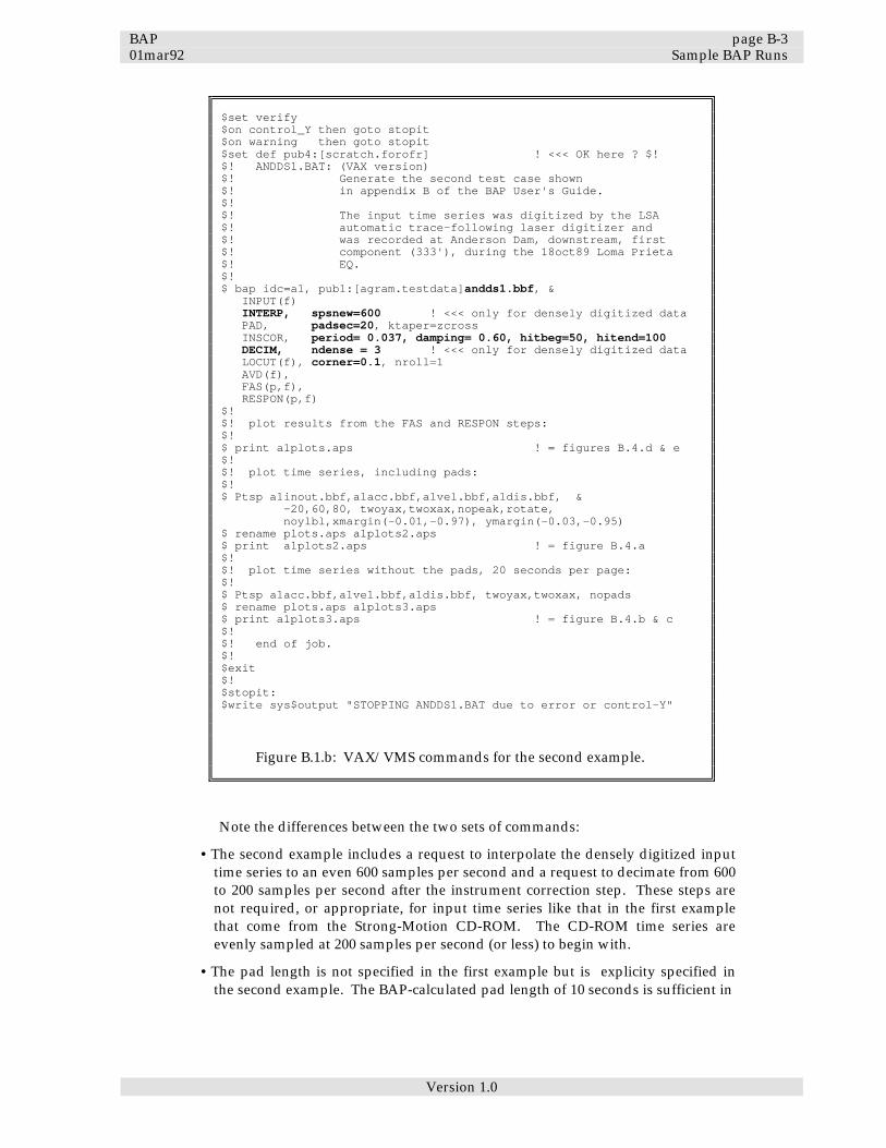
BAP page B-3 01mar92 Sample BAP Runs
Version 1.0
$set verify $on control_Y then goto stopit $on warning then goto stopit $set def pub4:[scratch.forofr] ! <<< OK here ? $! $! ANDDS1.BAT: (VAX version) $! Generate the second test case shown $! in appendix B of the BAP User's Guide. $! $! The input time series was digitized by the LSA $! automatic trace-following laser digitizer and $! was recorded at Anderson Dam, downstream, first $! component (333'), during the 18oct89 Loma Prieta $! EQ. $! $ bap idc=a1, pub1:[agram.testdata]andds1.bbf, & INPUT(f) INTERP, spsnew=600 ! <<< only for densely digitized data PAD, padsec=20, ktaper=zcross INSCOR, period= 0.037, damping= 0.60, hitbeg=50, hitend=100 DECIM, ndense = 3 ! <<< only for densely digitized data LOCUT(f), corner=0.1, nroll=1 AVD(f), FAS(p,f), RESPON(p,f) $! $! plot results from the FAS and RESPON steps: $! $ print a1plots.aps ! = figures B.4.d & e $! $! plot time series, including pads: $! $ Ptsp a1inout.bbf,a1acc.bbf,a1vel.bbf,a1dis.bbf, & -20,60,80, twoyax,twoxax,nopeak,rotate, noylbl,xmargin(-0.01,-0.97), ymargin(-0.03,-0.95) $ rename plots.aps a1plots2.aps $ print a1plots2.aps ! = figure B.4.a $! $! plot time series without the pads, 20 seconds per page: $! $ Ptsp a1acc.bbf,a1vel.bbf,a1dis.bbf, twoyax,twoxax, nopads $ rename plots.aps a1plots3.aps $ print a1plots3.aps ! = figure B.4.b & c $! $! end of job. $! $exit $! $stopit: $write sys$output "STOPPING ANDDS1.BAT due to error or control-Y"
Figure B.1.b: VAX/VMS commands for the second example.
Note the differences between the two sets of commands:
• The second example includes a request to interpolate the densely digitized input time series to an even 600 samples per second and a request to decimate from 600 to 200 samples per second after the instrument correction step. These steps are not required, or appropriate, for input time series like that in the first example that come from the Strong-Motion CD-ROM. The CD-ROM time series are evenly sampled at 200 samples per second (or less) to begin with.
• The pad length is not specified in the first example but is explicity specified in
the second example. The BAP-calculated pad length of 10 seconds is sufficient in

page B-4 BAP Sample BAP Runs 01mar92
Version 1.0
the first example, but the BAP-calculated pad length of 15 seconds is not sufficiently long for the second example, so the 20-second pad length must be specified by the user in the second example.
• The period, damping, hitbeg, hitend, corner, and nroll values are
given explicitly in the second example because the values are not available from the input time series file used in that example, as they are in the input file for the first example.
• The transition band for the high-cut filter is different in the two examples: 23 to
25 Hz in the first example (as is indicated in the input file) and 50 to 100 Hz in the second example (as is explicitly indicated in the BAP run parameters list). Refer to Section 5.2 of Chapter 5 for more information.
• The corner frequency for the low-cut filter is different in the two examples: 0.15
Hz in the first example (as is indicated in the input file), and 0.1 Hz in the second example (as is explicitly indicated in the BAP run parameters list). The appropriate value for this parameter will vary with each individual record. Refer to Section 5.6 of Chapter 5 for more information.
B.2 PC/DOS Commands B.2.a PC/DOS Commands for the First Example The following commands, similar to those shown in Figure B.1.a, could be typed in response to the DOS prompt (shown as "dos>" here) to run the first example on a PC/DOS machine: dos> bap idc=g1, pub1:[agram.testdata]gilroy21.smc, & INPUT(f), PAD, INSCOR, LOCUT(f), AVD(f), FAS(p,f), RESPON(p,f), DONE dos> print g1plots.aps dos> Ptsp g1inout.bbf,g1acc.bbf,g1vel.bbf,g1dis.bbf,-10,38,48 & twoyax,twoxax,nopeak,rotate, noylbl,xmargin(-0.01,-0.97), ymargin(-0.03,-0.95) done dos> rename plots.aps g1plots2.aps dos> print g1plots2.aps dos> Ptsp g1acc.bbf,g1vel.bbf,g1dis.bbf, twoyax,twoxax, nopads dos> rename plots.aps g1plots3.aps dos> print g1plots3.aps It is usually more convenient to run a rather long set of commands like these from a "batch" file (a .bat file) rather than to type them in at the DOS prompt. The contents of a batch file can be rerun repeatedly, with the user modifying the batch file between runs. Unfortunately, the "&" symbol cannot be used at the end of a long DOS command line within a batch file to request that DOS continue reading from the next line in the batch file, so DOS commands in batch files are limited to just one line each. The BAP run parameters list will often be too long to fit within the 128-character DOS command line limit: although the run parameter list in this first example would fit on one line, the run parameter list for the second example would not fit. A user wishing to run something like these examples from a batch file would need to use a separate @-file to contain the run parameters that would not fit on the BAP command line. The same is true for the information on the first PTSP command line in the examples. The gilroy21.bat file that is distributed with the BAP software illustrates how this can be done. The following is a simplified version (error handling removed) of gilroy21.bat:

BAP page B-5 01mar92 Sample BAP Runs
Version 1.0
: : Gilroy21.bat: (PC version) : generate the Gilroy Array #2 test case shown : in appendix B of the BAP User's Guide. : BAP idc=g1, c:\agram\testdata\gilroy21.smc, @gilroy21.brp print g1plots.aps PTSP g1inout.bbf,g1acc.bbf,g1vel.bbf,g1dis.bbf, @a.tsp rename plots.aps one.aps print one.aps PTSP g1acc.bbf,g1vel.bbf,g1dis.bbf, twoyax,twoxax, nopads print plots.aps
Note the "@gilroy21.brp" on the BAP command line and the "@a.tsp" on the first PTSP command in gilroy21.bat. Each @-sign indicates a file that contains additional input parameters. The contents of the gilroy21.brp file are: INPUT(f) PAD, ! << pad length will be calculated by BAP. INSCOR, ! << period, damping, hitbeg, & hitend ! will all come from the ts file. LOCUT(f), ! << corner & nroll will come from the ts file. AVD(f), FAS(p,f), RESPON(p,f)
And the contents of the a.tsp file referenced from the first PTSP command line are: twoyax,twoxax,nopeak,noylbl,portrait, xmargin(-0.01,-0.97), ymargin(-0.03,-0.95)
B.2.b PC/DOS Commands for the Second Example The andds1.bat file that is distributed with the BAP software illustrates how the second example could be executed from a PC/DOS batch file. The following is a simplified version of andds1.bat: : : ANDDS1.BAT: (PC version) : generate the Anderson downstream test case shown : in appendix B of the BAP User's Guide. : BAP idc=a1, c:\agram\testdata\andds1.bbf, @andds1.brp print a1plots.aps PTSP a1inout.bbf,a1acc.bbf,a1vel.bbf,a1dis.bbf, -50,100,150, @a.tsp rename plots.aps one.aps print one.aps PTSP a1acc.bbf,a1vel.bbf,a1dis.bbf, twoyax,twoxax, nopads print plots.aps Where contents of the andds.brp file referenced on the BAP command line are: INPUT(f) INTERP, spsnew=600 ! <<< only for densely digitized data PAD, padsec=20, ktaper=zcross INSCOR, period= 0.037, damping= 0.60, hitbeg=50, hitend=100 DECIM, ndense = 3 ! <<< only for densely digitized data LOCUT(f), corner=0.1, nroll=1 AVD(f), FAS(p,f), RESPON(p,f) And the a.tsp file referenced on the first PTSP command line is the same a.tsp file listed in Section B.2.a: twoyax,twoxax,nopeak,noylbl,portrait, xmargin(-0.01,-0.97), ymargin(-0.03,-0.95)

page B-6 BAP Sample BAP Runs 01mar92
Version 1.0
B.3 Results from the First Example The plots generated when the commands shown in Figure B.1.a were invoked are shown in Figures B.3.a through B.3.e. Figure B.3.a shows the plot generated by the first PTSP command: the entire input time series plus the resulting corrected acceleration, velocity, and displacement time series, including leading and trailing pads, are shown on a single page. Figures B.3.b and .c show the two plots generated by the second PTSP command. This plot is similar to the time series plots presented in the data reports published by the USGS: the corrected acceleration, velocity, and displacement time series are shown without the leading or trailing pads and with 20 seconds of motion on each page. Figures B.3.d and B.3.e show the two plots described in the g1plots.aps file that was generated by the BAP command. The plot in Figure B.3.d shows the Fourier amplitude spectrum of the acceleration time series; it was requested via the FAS(p) statement in the BAP run parameters list. The plot in figure B.3.e shows response spectra for 5 different damping fractions; it was requested via the RESPON(p) statement in the BAP run parameters list. The run messages BAP generated as it was executing this first (gilroy21) example were displayed on the user's screen and were also copied to the file named g1run.msg. Here follows a print-out of the g1run.msg file: BAP, Basic Accelerogram Processing Program, 10may92 version. IDC = G1, Run time =11may92@10:33:43 Input time-series file = PUB1:[AGRAM.TESTDATA]GILROY21.SMC Directory to contain output files = [] INPUT time series (input format = SMC) ================= Characteristics of the input time series: cm/sec/sec seconds sample # ---------- ------- -------- Max. acceleration = 239.95 3.2200 645 Min. acceleration = -249.62 3.6550 732 First sample = -2.8439 0.00000E+00 1 Last sample = -1.7474 26.855 5372 Sampling interval = 5.00000E-03 Output time series data file format = BBF, file name = G1INOUT.BBF PADding step, Part 1 (jpad=5, ktaper=zcross) ============ BAP-calculated leading pad length= 10. seconds. BAP-calculated trailing pad length= 10. seconds. Length of preliminary pads for the HICUT filter= 2.0 seconds. The time series has been extended with 400 leading zeros. In addition, the first 3 input samples were reset to zero. The time series has been extended with 400 trailing zeros. In addition, the last 8 input samples were reset to zero. cm/sec/sec seconds sample # ---------- ------- -------- Max. acceleration = 239.95 3.2200 1045 Min. acceleration = -249.62 3.6550 1132 First pad sample = 0.00000E+00 -2.0000 1 First data sample = 0.00000E+00 0.00000E+00 401 Last data sample = 0.00000E+00 26.855 5772 Last pad sample = 0.00000E+00 28.855 6172 Sampling interval = 5.00000E-03 INStrument CORrection and HIgh-CUT filter steps =============================================== Instrument period = 0.038 seconds,

BAP page B-7 01mar92 Sample BAP Runs
Version 1.0
Instrument damping fraction = 0.600 of critical damping, Filter transition band = 23.0 to 25.0 Hz. cm/sec/sec seconds sample # ---------- ------- -------- Max. acceleration = 236.51 3.2050 1042 Min. acceleration = -250.03 3.6450 1130 First pad sample = 5.72205E-05 -2.0000 1 First data sample = -0.23041 0.00000E+00 401 Last data sample = 2.78170E-02 26.855 5772 Last pad sample = -1.90735E-06 28.855 6172 Sampling interval = 5.00000E-03 PADding step, Part 2 (jpad=4, using zcross on existing pad) ============ The time series has been extended with 1600 leading zeros. The time series has been extended with 1600 trailing zeros. cm/sec/sec seconds sample # ---------- ------- -------- Max. acceleration = 236.51 3.2050 2642 Min. acceleration = -250.03 3.6450 2730 First pad sample = 0.00000E+00 -10.000 1 First data sample = -0.23041 0.00000E+00 2001 Last data sample = 2.78170E-02 26.855 7372 Last pad sample = 0.00000E+00 36.855 9372 Sampling interval = 5.00000E-03 LOCUT filter step (corner= 0.15, nroll= 1) ================= Filter the acceleration time series with a low-cut, bi-directional Butterworth filter having corner frequency at 0.150 Hz and rolloff parameter = 1. (Note that rolloff parameter= 1 is also known as a rolloff "order" of 2.) cm/sec/sec seconds sample # ---------- ------- -------- Max. acceleration = 235.79 3.2050 2642 Min. acceleration = -250.49 3.6450 2730 First pad sample = -1.26688E-04 -10.000 1 First data sample = -0.33074 0.00000E+00 2001 Last data sample = 0.23881 26.855 7372 Last pad sample = 3.89814E-04 36.855 9372 Sampling interval = 5.00000E-03 Output time series data file format = BBF, file name = G1ACC.BBF AVD step ======== Integrate the acceleration time series once to calculate velocity, twice to calculate displacement. Velocity: cm/sec seconds sample # ---------- ------- -------- Max. velocity = 31.916 3.5700 2715 Min. velocity = -28.590 3.0200 2605 First pad sample = -3.16720E-07 -10.000 1 First data sample = -8.93613E-02 0.00000E+00 2001 Last data sample = -0.17900 26.855 7372 Last pad sample = 7.31175E-05 36.855 9372 Sampling interval = 5.00000E-03 Output time series data file format = BBF, file name = G1VEL.BBF Displacement: cm seconds sample # ---------- ------- -------- Max. displacement = 2.3500 4.0250 2806 Min. displacement = -5.5289 3.2250 2646 First pad sample = -7.91801E-10 -10.000 1 First data sample = -1.80094E-02 0.00000E+00 2001 Last data sample = 3.38164E-02 26.855 7372 Last pad sample = 3.43564E-03 36.855 9372 Sampling interval = 5.00000E-03 Output time series data file format = BBF, file name = G1DIS.BBF FAS step ======== Calculate Fourier amplitude spectrum of acceleration. The time series has been extended with 7012 trailing zeros so the total number of samples is an integral power of 2 (= 16384) as is required for the FFT used in the
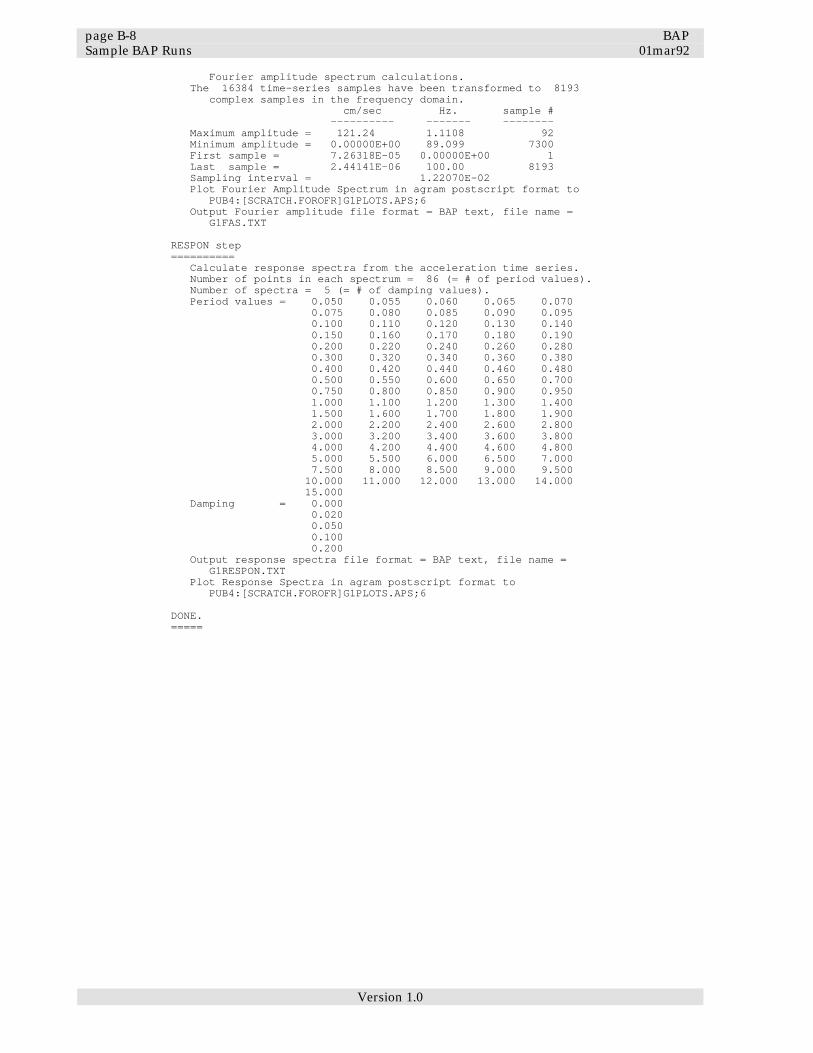
page B-8 BAP Sample BAP Runs 01mar92
Version 1.0
Fourier amplitude spectrum calculations. The 16384 time-series samples have been transformed to 8193 complex samples in the frequency domain. cm/sec Hz. sample # ---------- ------- -------- Maximum amplitude = 121.24 1.1108 92 Minimum amplitude = 0.00000E+00 89.099 7300 First sample = 7.26318E-05 0.00000E+00 1 Last sample = 2.44141E-06 100.00 8193 Sampling interval = 1.22070E-02 Plot Fourier Amplitude Spectrum in agram postscript format to PUB4:[SCRATCH.FOROFR]G1PLOTS.APS;6 Output Fourier amplitude file format = BAP text, file name = G1FAS.TXT RESPON step ========== Calculate response spectra from the acceleration time series. Number of points in each spectrum = 86 (= # of period values). Number of spectra = 5 (= # of damping values). Period values = 0.050 0.055 0.060 0.065 0.070 0.075 0.080 0.085 0.090 0.095 0.100 0.110 0.120 0.130 0.140 0.150 0.160 0.170 0.180 0.190 0.200 0.220 0.240 0.260 0.280 0.300 0.320 0.340 0.360 0.380 0.400 0.420 0.440 0.460 0.480 0.500 0.550 0.600 0.650 0.700 0.750 0.800 0.850 0.900 0.950 1.000 1.100 1.200 1.300 1.400 1.500 1.600 1.700 1.800 1.900 2.000 2.200 2.400 2.600 2.800 3.000 3.200 3.400 3.600 3.800 4.000 4.200 4.400 4.600 4.800 5.000 5.500 6.000 6.500 7.000 7.500 8.000 8.500 9.000 9.500 10.000 11.000 12.000 13.000 14.000 15.000 Damping = 0.000 0.020 0.050 0.100 0.200 Output response spectra file format = BAP text, file name = G1RESPON.TXT Plot Response Spectra in agram postscript format to PUB4:[SCRATCH.FOROFR]G1PLOTS.APS;6 DONE. =====

BAP page B-9 01mar92 Sample BAP Runs
Version 1.0
Figure B.3.a

page B-10 BAP Sample BAP Runs 01mar92
Version 1.0
Figure B.3.b
Figure B.3.c

BAP page B-11 01mar92 Sample BAP Runs
Version 1.0
Figure B.3.d
Figure B.3.e
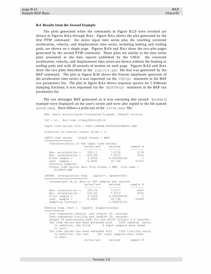
page B-12 BAP Sample BAP Runs 01mar92
Version 1.0
B.4 Results from the Second Example The plots generated when the commands in Figure B.2.b were invoked are shown in Figures B.4.a through B.4.e. Figure B.4.a shows the plot generated by the first PTSP command: the entire input time series plus the resulting corrected acceleration, velocity, and displacement time series, including leading and trailing pads, are shown on a single page. Figures B.4.b and B.4.c show the two plot pages generated by the second PTSP command. These plots are similar to the time series plots presented in the data reports published by the USGS: the corrected acceleration, velocity, and displacement time series are shown without the leading or trailing pads and with 20 seconds of motion on each page. Figures B.4.d and B.4.e show the two plots described in the a1plots.aps file that was generated by the BAP command. The plot in Figure B.3d shows the Fourier amplitude spectrum of the acceleration time series; it was requested via the FAS(p) statement in the BAP run parameters list. The plot in figure B.4.e shows response spectra for 5 different damping fractions; it was requested via the RESPON(p) statement in the BAP run parameters list. The run messages BAP generated as it was executing this second (andds1) example were displayed on the user's screen and were also copied to the file named a1run.msg. Here follows a print-out of the a1run.msg file: BAP, Basic Accelerogram Processing Program, 10may92 version. IDC = A1, Run time =11may92@10:48:39 Input time-series file = PUB1:[AGRAM.TESTDATA]ANDDS1.BBF Directory to contain output files = [] INPUT time series (input format = BBF) ================= Characteristics of the input time series: cm/sec/sec seconds sample # ---------- ------- -------- Max. acceleration = 240.11 7.6718 5178 Min. acceleration = -243.00 7.8707 5310 First sample = 3.4369 0.00000E+00 1 Last sample = -5.6083 39.748 27314 Unevenly sampled. - Output time series data file format = BBF, file name = A1INOUT.BBF INTERP, interpolation step (spsin=*, spsnew=600) ========================== Interpolate (x,y) data to 600 samples per second: cm/sec/sec seconds sample # ---------- ------- -------- Max. acceleration = 240.04 7.6717 4604 Min. acceleration = -242.82 7.8717 4724 First sample = 3.4369 0.00000E+00 1 Last sample = -5.6088 39.748 23850 Sampling interval = 1.66667E-03 PADding step, Part 1 (jpad=5, ktaper=zcross) ============ User-requested leading pad length= 20. seconds. User-requested trailing pad length= 20. seconds. Length of preliminary pads for the HICUT filter= 2.0 seconds. The time series has been extended with 1200 leading zeros. In addition, the first 4 input samples were reset to zero. The time series has been extended with 1200 trailing zeros. In addition, the last 341 input samples were reset to zero. cm/sec/sec seconds sample #

BAP page B-13 01mar92 Sample BAP Runs
Version 1.0
---------- ------- -------- Max. acceleration = 240.04 7.6717 5804 Min. acceleration = -242.82 7.8717 5924 First pad sample = 0.00000E+00 -2.0000 1 First data sample = 0.00000E+00 0.00000E+00 1201 Last data sample = 0.00000E+00 39.748 25050 Last pad sample = 0.00000E+00 41.748 26250 Sampling interval = 1.66667E-03 INStrument CORrection and HIgh-CUT filter steps =============================================== Instrument period = 0.037 seconds, Instrument damping fraction = 0.600 of critical damping, Filter transition band = 50.0 to 100.0 Hz. cm/sec/sec seconds sample # ---------- ------- -------- Max. acceleration = 238.26 7.6717 5804 Min. acceleration = -238.38 7.8617 5918 First pad sample = 2.38419E-07 -2.0000 1 First data sample = -0.25486 0.00000E+00 1201 Last data sample = -2.54502E-06 39.748 25050 Last pad sample = -2.31806E-08 41.748 26250 Sampling interval = 1.66667E-03 DECIMate, decimation step (ndense= 3) ========================= Remove 2 of every 3 samples to reduce the sampling rate to 200.000 samples per second. cm/sec/sec seconds sample # ---------- ------- -------- Max. acceleration = 237.86 7.6700 1935 Min. acceleration = -237.64 7.8650 1974 First pad sample = 2.38419E-07 -2.0000 1 First data sample = -0.25486 0.00000E+00 401 Last data sample = -4.25649E-07 39.745 8350 Last pad sample = 3.28096E-08 41.745 8750 Sampling interval = 5.00000E-03 PADding step, Part 2 (jpad=4, using zcross on existing pad) ============ The time series has been extended with 3600 leading zeros. The time series has been extended with 3600 trailing zeros. In addition, the last 3 samples of the existing trailing pad were reset to zero. cm/sec/sec seconds sample # ---------- ------- -------- Max. acceleration = 237.86 7.6700 5535 Min. acceleration = -237.64 7.8650 5574 First pad sample = 0.00000E+00 -20.000 1 First data sample = -0.25486 0.00000E+00 4001 Last data sample = -4.25649E-07 39.745 11950 Last pad sample = 0.00000E+00 59.745 15950 Sampling interval = 5.00000E-03 LOCUT filter step (corner= 0.1, nroll= 1) ================= Filter the acceleration time series with a low-cut, bi-directional Butterworth filter having corner frequency at 0.100 Hz and rolloff parameter = 1. (Note that rolloff parameter= 1 is also known as a rolloff "order" of 2.) cm/sec/sec seconds sample # ---------- ------- -------- Max. acceleration = 236.32 7.6700 5535 Min. acceleration = -239.09 7.8650 5574 First pad sample = -5.03567E-05 -20.000 1 First data sample = -6.04142E-02 0.00000E+00 4001 Last data sample = -0.18701 39.745 11950 Last pad sample = 7.65612E-05 59.745 15950 Sampling interval = 5.00000E-03 Output time series data file format = BBF, file name = A1ACC.BBF AVD step ======== Integrate the acceleration time series once to calculate velocity, twice to calculate displacement. Velocity: cm/sec seconds sample # ---------- ------- -------- Max. velocity = 19.198 8.4150 5684

page B-14 BAP Sample BAP Runs 01mar92
Version 1.0
Min. velocity = -18.528 3.8900 4779 First pad sample = -1.25892E-07 -20.000 1 First data sample = -0.21296 0.00000E+00 4001 Last data sample = 0.27848 39.745 11950 Last pad sample = 2.05285E-05 59.745 15950 Sampling interval = 5.00000E-03 Output time series data file format = BBF, file name = A1VEL.BBF Displacement: cm seconds sample # ---------- ------- -------- Max. displacement = 6.6759 3.5050 4702 Min. displacement = -5.5133 6.3350 5268 First pad sample = -3.14730E-10 -20.000 1 First data sample = -0.97244 0.00000E+00 4001 Last data sample = -0.15190 39.745 11950 Last pad sample = 1.57040E-03 59.745 15950 Sampling interval = 5.00000E-03 Output time series data file format = BBF, file name = A1DIS.BBF FAS step ======== Calculate Fourier amplitude spectrum of acceleration. The time series has been extended with 434 trailing zeros so the total number of samples is an integral power of 2 (= 16384) as is required for the FFT used in the Fourier amplitude spectrum calculations. The 16384 time-series samples have been transformed to 8193 complex samples in the frequency domain. cm/sec Hz. sample # ---------- ------- -------- Maximum amplitude = 245.09 1.6235 134 Minimum amplitude = 8.84059E-06 99.939 8188 First sample = 2.07520E-05 0.00000E+00 1 Last sample = 8.81958E-05 100.00 8193 Sampling interval = 1.22070E-02 Plot Fourier Amplitude Spectrum in agram postscript format to PUB4:[SCRATCH.FOROFR]A1PLOTS.APS;5 Output Fourier amplitude file format = BAP text, file name = A1FAS.TXT RESPON step ========== Calculate response spectra from the acceleration time series. Number of points in each spectrum = 86 (= # of period values). Number of spectra = 5 (= # of damping values). Period values = 0.050 0.055 0.060 0.065 0.070 0.075 0.080 0.085 0.090 0.095 0.100 0.110 0.120 0.130 0.140 0.150 0.160 0.170 0.180 0.190 0.200 0.220 0.240 0.260 0.280 0.300 0.320 0.340 0.360 0.380 0.400 0.420 0.440 0.460 0.480 0.500 0.550 0.600 0.650 0.700 0.750 0.800 0.850 0.900 0.950 1.000 1.100 1.200 1.300 1.400 1.500 1.600 1.700 1.800 1.900 2.000 2.200 2.400 2.600 2.800 3.000 3.200 3.400 3.600 3.800 4.000 4.200 4.400 4.600 4.800 5.000 5.500 6.000 6.500 7.000 7.500 8.000 8.500 9.000 9.500 10.000 11.000 12.000 13.000 14.000 15.000 Damping = 0.000 0.020 0.050 0.100 0.200 Output response spectra file format = BAP text, file name = A1RESPON.TXT Plot Response Spectra in agram postscript format to PUB4:[SCRATCH.FOROFR]A1PLOTS.APS;5 DONE. =====

BAP page B-15 01mar92 Sample BAP Runs
Version 1.0
Figure B.4.a

page B-16 BAP Sample BAP Runs 01mar92
Version 1.0
Figure B.4.b
Figure B.4.c

BAP page B-17 01mar92 Sample BAP Runs
Version 1.0
Figure B.4.d
Figure B.4.e

page B-18 BAP Sample BAP Runs 01mar92
Version 1.0
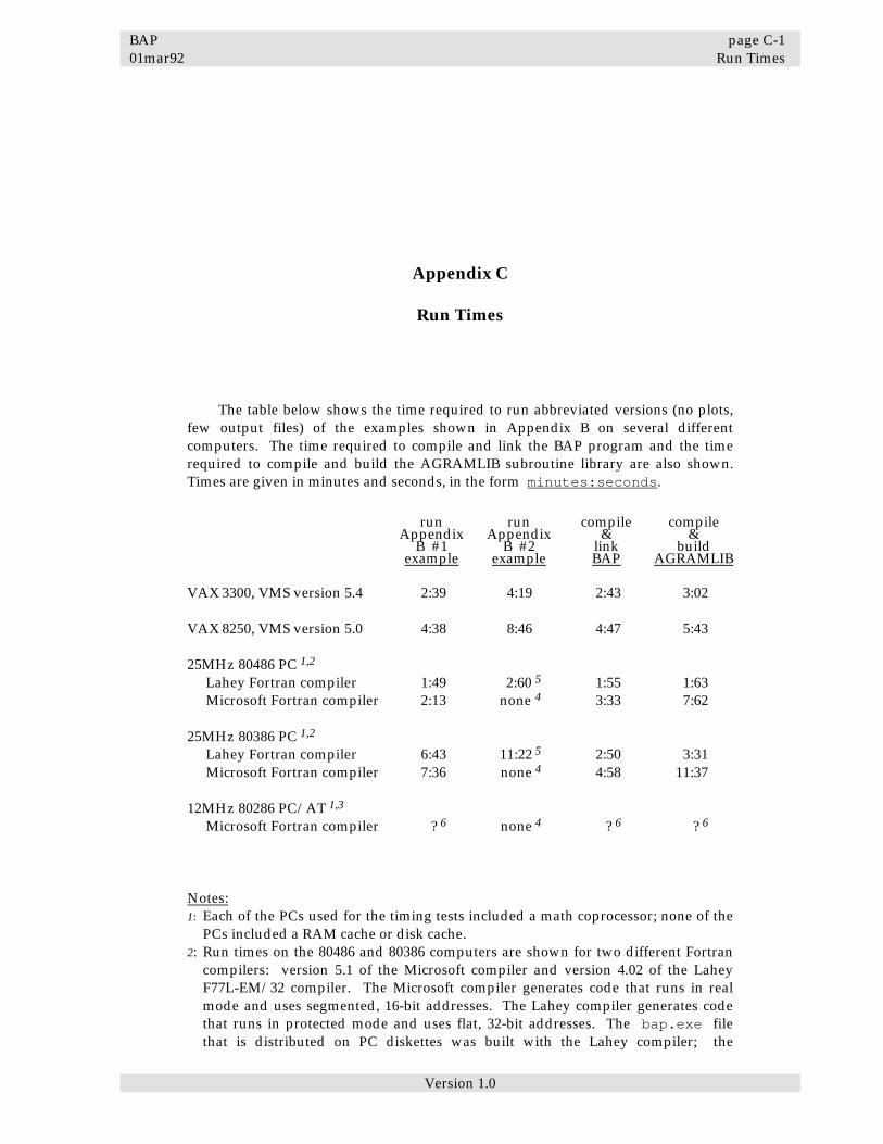
BAP page C-1 01mar92 Run Times
Version 1.0
Appendix C
Run Times The table below shows the time required to run abbreviated versions (no plots, few output files) of the examples shown in Appendix B on several different computers. The time required to compile and link the BAP program and the time required to compile and build the AGRAMLIB subroutine library are also shown. Times are given in minutes and seconds, in the form minutes:seconds. run run compile compile Appendix Appendix & & B #1 B #2 link build example example BAP AGRAMLIB VAX 3300, VMS version 5.4 2:39 4:19 2:43 3:02 VAX 8250, VMS version 5.0 4:38 8:46 4:47 5:43 25MHz 80486 PC 1,2 Lahey Fortran compiler 1:49 2:60 5 1:55 1:63 Microsoft Fortran compiler 2:13 none 4 3:33 7:62 25MHz 80386 PC 1,2 Lahey Fortran compiler 6:43 11:22 5 2:50 3:31 Microsoft Fortran compiler 7:36 none 4 4:58 11:37 12MHz 80286 PC/AT 1,3 Microsoft Fortran compiler ? 6 none 4 ? 6 ? 6 Notes: 1: Each of the PCs used for the timing tests included a math coprocessor; none of the
PCs included a RAM cache or disk cache. 2: Run times on the 80486 and 80386 computers are shown for two different Fortran
compilers: version 5.1 of the Microsoft compiler and version 4.02 of the Lahey F77L-EM/32 compiler. The Microsoft compiler generates code that runs in real mode and uses segmented, 16-bit addresses. The Lahey compiler generates code that runs in protected mode and uses flat, 32-bit addresses. The bap.exe file that is distributed on PC diskettes was built with the Lahey compiler; the
page C-2 BAP Run Times 01mar92
Version 1.0
lowbap.exe file and all the .exe files for the support programs were built with the Microsoft compiler.
3: Run times for the 80286 computer are shown merely to illustrate that the BAP program requires faster machines to run in a reasonable length of time. The .exe files given in the PC BAP distribution set will not run on these computers. The 32-bit version of the Lahey compiler (the F77L-32/EM compiler) will not generate code for 80286 or 8086 computers. Although the Microsoft compiler can generate code for 80286s and 8086s, such code is not included among the BAP distribution files.
4: The Microsoft-compiled version of BAP (lowbap.exe) limits (truncates) the time series it can deal with to 16K samples; that's 80 seconds of an evenly-sampled, 200-sample-per-second time series. This is not long enough to handle the padded time series used in the second Appendix B example.
5: Most the time spent running the two Appendix B examples is spent in the RESPON step. The RESPON calculations make heavy use of floating-point functions, which are more efficient on 80486 computers than on 80386 computers.
6: These test cases have not been run on a 286 yet. Once the information is available, it will be given in the bapinfo.txt file (see Appendix D).
BAP page D-1 01mar92 Acquiring BAP Software
Version 1.0
Appendix D
Acquiring the BAP software The preliminary version of PC/BAP and its support programs is distributed on 3.5-inch, 1.44M PC diskettes as Open-File Report # 92-296B by the Open-File Reports Section of the USGS. The telephone and mailing address for the Open-File Reports Section are given on the back of the title page of this report. Future versions of the programs will probably be distributed by other means, however (see Reference [23]). Users can receive information about the current status of the programs and their distribution methods by requesting a print-out of the current version of bapinfo.txt from the author of this report. The bapinfo.txt file will provide information about the current version of BAP, its support programs, documentation, and availability that is not covered in this report. To request a print-out of bapinfo.txt, send a self-addressed envelope to the author at the address given on the preface page. U.S. residents please add postage (2 first-class stamps) to the envelope. Source code for BAP and its support programs is available for other-than-PC computers on 9-track tape. Until such time as 9-track tape copies of the software are available from formal distribution sources, users may request a copy from the author. A 9-track tape and a return mailing label should be mailed with such a request. Note that the files distributed on 9-track tape include source code only, in contrast to the PC distribution diskettes, which contain executable files as well as source code. BAP is a new program and will almost certainly be updated in the future if the USGS allocates time and funding to the effort. An update history is included in the bapinfo.txt file, so it is important for users to request a current copy of bapinfo.txt periodically. The bapinfo.txt file may be posted on a computer-based bulletin board eventually, if there is sufficient interest, but at present it is only available by requesting a print-out from the author by mail. Some of the additions that might be made to the software include: • PC versions of all the support programs listed in Chapter 6. • Versions of the programs for UNIX and MAC machines. • A version of the FASPLOT program that does not restrict (truncate) its input time
series to 16,000 samples or less. The present versions of all the support programs, including FASPLOT, are 16-bit, real-mode programs that must run within the 640K memory limit imposed by the DOS operating system. A 32-bit version of

page D-2 BAP Acquiring BAP Software 01mar92
Version 1.0
FASPLOT should be provided that makes use of the same DOS-extending software as is used by the BAP program. (The support programs were created with the Microsoft Fortran compiler; BAP was created with the Lahey F77L-32/EM compiler.)
• A program named RSPLOT that will plot pseudo-velocity response spectra in tri-
partite axes, given a baprspec.txt file generated by the BAP/RSPEC step. The program should provide various other response spectra plotting options too.
• More accurate integration and differentiation algorithms in the AVD step. • More formats for the BAP input and output time-series data files or more
reformatting functions in the IMPORT and EXPORT programs. The file format used for the data presented in Reference [15] (digital recordings of Loma Prieta after-shocks), should be among those BAP or IMPORT/EXPORT can accept. Formats used by the software associated with references [22] through [25] should also be acceptable to BAP or IMPORT/EXPORT.
• More flexibility in the plotting options in BAP. • Better character positioning in the PC screen plots. • Include VAX screen-plotting software with the VAX/BAP distribution files. • Plot description files in HPGL format, the format suited to Hewlett-Packard
Laserjet printers, in addition to the PostScript format that is available now. • Faster PostScript file processing. And the .aps PostScript file format should be
modified so the PostScript plot information files can be incorporated into Word Perfect documents, as they were into this document, which was formatted by Microsoft Word. (See sample plots in Chapter 5.)

BAP page E-1 01mar92 Installing PC BAP
Version 1.0
Appendix E
Installing BAP on IBM Personal Computers and Clones PC/BAP and its support programs require an IBM-style PC or "clone" having an 80386 CPU (or an upward-compatible CPU such as an 80486); an 80387 math coprocessor; and 3M bytes or more of RAM. Other required characteristics of the computer are listed in Section 1.4 of Chapter 1. The software is distributed for PCs in self-extracting archive files on 3.5", 720K floppy diskettes. (See Appendix D for information about BAP distribution methods.) The number and names of the files in the distribution set will vary, depending on when and from where they were acquired, but at the time this is written, there are six distribution files: File name Contents bapinfo.txt general information. (text file) bapinfo.ps PostScript version of bapinfo.txt. (text file in PostScript
format) bapexes1.exe BAP and LOWBAP executable files. (archive file) bapexes2.exe executable files for the support programs. (archive file) bapaux.exe auxiliary files such as the help file, examples, test data, and
miscellaneous documentation. (archive file) bapcode.exe the Fortran code and related files that were used to create the
executable files. (archive file) The number of distribution files and the names of the files, other than bapinfo.txt, will change as the software evolves, so it is important that users refer to the list of file names given in bapinfo.txt rather than the list given here when they prepare to install BAP and related programs. The bapinfo.txt file may provide a variety of information, in addition to the names of the distribution files, that is more current than that given here. Bapinfo.txt is a plain ASCII text file: It can be read with a text editor, or displayed with the DOS type command. Bapinfo.ps is the PostScript counterpart to bapinfo.txt: It can be printed on a PostScript printer. The .exe distribution files are self-extracting archive files: They contain a compact collection of other files that will be generated on the user's current disk and directory when the user types the name of the file at the DOS prompt. Note, however, that the user should usually type the "-d" and "-o" switches after the name of a self-extracting archive file when extracting the component files. Example:

page E-2 BAP Installing PC BAP 01mar92
Version 1.0
dos> a:bapexes1 -d -o The "-d" requests that component files be copied from the archive file into subdirectories below the current directory. The "-o" requests that any component file from the archive that has the same name as an existing file in the target directory will over-write the existing file. E.1 Installation Overview A brief overview of the installation process is given in this Section. These instructions should be adequate for many users, but they are presented as though the user wishes to install the software on the c: drive, that the distribution diskettes are inserted in the b: drive, that the computer uses a VGA or CGA video system, and that the computer's extended memory is not currently in use as a RAM drive or disk cache. More flexible and detailed instructions are given in the next Section. To install the software, first create a directory named \agram\ just below the root of the c: drive and set your current directory to be the newly-created c:\agram\ directory: dos> c: (set the current drive to c:) dos> md \agram (create the \agram\ directory) dos> cd \agram (set the current directory to \agram\) Next, transfer the component files from the self-extracting distribution archive files in the b: drive to subdirectories below the new c:\agram\ directory. Insert the appropriate diskette into the b: drive as needed and use the following commands: dos> b:bapexes1 -d -o (the -d is important!) dos> b:bapexes2 -d -o dos> b:bapaux -d -o dos> b:bapcode -d -o (this one is optional) dos> dir (use this just to check that you remembered
to type the -d on the above commands: if so, the current directory will contain subdirectories rather than files.)
Invoke the agram setup commands in the c:\agram\examples\4agram.bat file (you must do this every time you power up your computer, before you can use BAP or any of its support programs): dos> c:\agram\examples\4agram.bat That's all there is to it! You may want to verify that all has been installed properly by following some of the examples given in Section E.3, however. And you should probably skim though the information in Section E.2 even if the instructions in this Section were sufficient to allow you to install the software successfully.

BAP page E-3 01mar92 Installing PC BAP
Version 1.0
E.2 Installation steps 1) Read the bapinfo.txt file. A copy of bapinfo.txt will be on the first diskette in the distribution set. It
may contain instructions more recent than those given here. If the first diskette is inserted in drive b:, you can read bapinfo.txt by typing:
dos> type b:bapinfo.txt | more then pressing the space bar whenever you are ready to see the next screen full of
text. The instructions that follow show b: as the designator for the drive that
contains the distribution diskettes. The b: should be replaced with the designator for the drive in which you have actually placed those files, drive a: perhaps.
If you would rather read bapinfo.txt on paper rather than on the screen, you
can print the information on a PostScript printer with: dos> print b:bapinfo.ps (note the .ps) If your printer is not a PostScript printer, use: dos> print b:bapinfo.txt (note the .txt) 2) Set the "current" drive. Set the current drive to be the drive on which you want to install the programs
and related files. This drive should be a partition of a hard disk, rather than a floppy disk drive. To set the current drive to the c: drive, for instance, type "c:" at the DOS prompt:
dos> c: The instructions that follow show c: as the current drive. The c: should be
replaced with the designator for the drive on which you actually want the programs and related files to be installed, m: perhaps.
3) Verify that there is enough space on the hard disk. Use the dir command to verify that there is enough space on the current drive
for the new files you are about to copy to the disk: dos> dir The last line of the dir display will show the number of bytes of unused space
available on the drive. The bapinfo.txt file will indicate how many bytes are required for the BAP files, but at the time this is written, 5.5M bytes are required for all the BAP files and 3.5M bytes are required if the source files (the Fortran code and related files from the bapcode.exe file) are not included.
4) Set your "current" directory to be the parent directory for the new files. Create a directory to serve as the parent directory for the new files and
subdirectories, if the appropriate directory does not already exist. It is preferable that this directory be reserved for the BAP distribution files and that it not be used for any other files. If so, the contents of the directory can be deleted and reloaded whenever new versions of the BAP distribution files become available.

page E-4 BAP Installing PC BAP 01mar92
Version 1.0
To create a directory named agram below the root directory of the current drive, type:
dos> md \agram (Note that there is no trailing backslash here.) The instructions that follow show c:\agram\ as the parent directory for the
new files. The \agram\ characters should be replaced with the name of the directory in which you actually want the programs and related files to be installed, \pgms\usgs\bapstuff\ perhaps. It is best to use agram as the parent directory name, however, for \agram\ is indicated throughout this report, the help file, and the diagnostic messages as the parent directory for BAP and AGRAM-related files. The name used is "AGRAM" rather than "BAP" for consistency with the way the files are arranged on the USGS computers, where BAP is a member of a group of programs collectively called AGRAM programs.
If the c:\agram\ directory already exists -- because you are installing an
updated version of the software, perhaps -- it is best to delete all the files in the directory and in all its subdirectories before proceding to install the new version of the sofware. (It is not mandatory, however.)
Next, set your current directory to be the new (or newly emptied) directory. To
set your current directory to \agram\, type: dos> cd \agram 5) Transfer the new files from the diskettes to your hard disk. Each distribution diskette will contain one or more of the .exe files indicated
on the first page of this Appendix. For each diskette, insert the diskette into drive b:, use the DIR command to learn the name(s) of the .exe file(s) on the diskette, then transfer the component files from the .exe file(s) on diskette to your hard disk:
dos> dir b:*.exe dos> b:whatever -d -o where whatever is the name of an .exe file currently in the b: drive. If the
DIR command showed that the diskette in b: contained the file named bapexes1.exe, for example, then you would use:
dos> b:bapexes1 -d -o to do the transfer. If the floppies are inserted, as needed, into drive b:, you will
use (in no particular order): dos> b:bapexes1 -d -o (the -d is important!) dos> b:bapexes2 -d -o dos> b:bapaux -d -o And, if you want the Fortran code: dos> b:bapcode -d -o The "-d" and "-o" are important! The -d indicates that the new files should
be arranged in subdirectories below your current directory rather than all together in your current directory. The -o indicates that new files should overwrite any existing files in the destination directories. The -o is unnecessary
BAP page E-5 01mar92 Installing PC BAP
Version 1.0
the first time you install the software or if you install the software in an empty directory, but is needed if you reinstall new versions of the files in place of older versions.
The above commands will copy a variety of BAP and AGRAM-related files into
subdirectories below your current directory on your hard drive. Information about the various files and subdirectories is given in Section E.5.
Note that the b:bapcode.exe archive file contains Fortran code and related
files required to reconstruct the executable files. You do not need to store these files on your hard disk until and unless you intend to alter one of the programs. When unarchived, the files from b:bapcode.exe fill up 2M bytes of disk space.
6) Display the contents of your current directory. Use the DIR command to make certain that the distribution files were transfered
to subdirectories below the current directory rather than into the current directory itself:
dos> dir The resulting display should show that the current directory is c:\agram and
that there are very few files therein: a read.me file, the "." and ".." files, and several subdirectories (for which a "<DIR>" will be shown in the second column of the display).
It is very easy to forget to type the "-d" in your archive extraction commands
(step 5), and as a consequence, have some or all of the distribution files transfered to your current directory rather than into subdirectories below that directory. In that case, the DIR display will show many files: You should delete these files and repeat step 5, remembering to type the "-d" this time!
7) Execute the 4agram.bat setup commands. Create a 4agram.bat file that you will invoke whenever you wish to run BAP
or its auxiliary software. The 4agram.bat file should contain the following two statements:
set agroot=c:\agram path=%agroot%\exes;%path% and possibly a third statement: c:\agram\exes\msherc The first statement defines a new environment variable named agroot that
indicates the parent directory below which all the BAP distribution files are located. The second statement adds the c:\agram\exes directory to the DOS path environment variable. (Note that this second statement must be executed from within a .bat file: the %whatever% syntax will not work as intended if typed at the DOS command line.) The third statement should be included if and only if your computer uses a monochrome, Hercules-compatible monitor and video adaptor.
To invoke the 4agram.bat setup commands, either: A) If you have genuinely installed the distribution files at c:\agram rather
than on some other partition or directory, and if you are not using a Hercules-compatible monochrome monitor, you can use the 4agram.bat

page E-6 BAP Installing PC BAP 01mar92
Version 1.0
file that is provided among the distribution files. To invoke it, simply type the following at the DOS prompt:
dos> c:\agram\examples\4agram.bat or B) If you have installed the programs on a disk partition and directory other
than c:\agram, however, or you are using a Hercules monitor, you will need to make a copy of the distributed 4agram.bat file, then use a text editor (or the character-only mode of a word processor) to modify your copy of 4agram.bat. Change the "c:\agram" therein to the appropriate drive designator and directory and/or remove the leading comments from the "c:\agram\exes\msherc" line.
You will probably want to place your 4agram.bat file in some directory
that is listed in your DOS path environment variable, so you will not need to type the path to the file each time you invoke 4agram.bat. And, if you've modified 4agram.bat, it is best to keep your copy of 4agram.bat in some directory other than \agram or its subdirectories, so you can install new versions of this software, when they become available, without overwriting your special version of 4agram.bat. Or, you may want to include the commands in 4agram.bat within your autoexec.bat file (See step 9a).
Once you have modified your copy of 4agram.bat, invoke the commands
therein: dos> 4agram.bat Warning: 4agram.bat may lock up your computer or generate diagnostic
messages ("out of environment space", "path too long", "bad command or file name"). If so, refer to Sections F.10 and F.11 in the Trouble-Shooting Appendix.
To verify that 4agram.bat has defined the agroot environment variable
without adding any trailing blanks, use the path command without any arguments:
dos> path This will display the current value for the path environment variable, as it has
been modified by 4agram.bat. Users who have modified their own version of 4agram.bat could easily, and unknowingly, have introduced trailing blanks to the end of some of the lines in the modified 4agram.bat, thanks to quirks in some text editors that occasionally add the trailing blanks. And trailing blanks at the end of the agroot value will cause problems! If the path value displayed shows any blanks between the "c:\agram" and the "\exes;", you will need to remove the trailing blank(s) from the set agroot=c:\agram statement in 4agram.bat.
8) Verify that the computer has been configured to allow BAP to use extended
memory. BAP runs in the "extended" memory area above the first 640K bytes of
"conventional" memory used by DOS, and as a consequence your computer must have at least 3M bytes of RAM in order to run BAP. The computer must be configured so that all or part of its extended memory is available to BAP rather than having all the extended memory put to use as a RAM disk or a disk cache. And any Extended-Memory Management software in use on the computer must

BAP page E-7 01mar92 Installing PC BAP
Version 1.0
be compatible with BAP. If RAM disks, disk caches, and Memory Managers are unfamiliar to you, they are probably not implemented on your computer and cannot, therefor, interfere with BAP -- unless someone else configured your computer for you.
If your computer is presently configured so that all its extended memory is used
as a RAM drive or as a disk cache, you will need to reconfigure the computer to make at least 2M bytes of the extended memory available to BAP. If your computer is configured so that part of its extended memory is used as a RAM drive or a disk cache, BAP will normally detect that fact and use only the extended memory that remains. Some RAM drive or disk-caching drivers cannot be detected by BAP, however, and these should be disabled whenever you use BAP. The MEM command that is provided with MS DOS, versions 4.0 and higher (but not with earlier versions of DOS), will report the total amount of extended or XMS1 memory that you have on your computer. The WHATMEM command that is provided with the BAP support programs will report how much of that extended or XMS memory it detects as being available for use by BAP. Try the following to learn about the extended memory on your computer:
dos> mem (this requires DOS version 4.0 or greater.) dos> whatmem If your computer is configured to use part of its extended memory as a RAM disk
or disk cache but WHATMEM reports that the same memory used by the RAM disk or disk cache is "available", you will need to disable the RAM disk or disk cache whenever you use BAP. Several RAM drive configurations and corresponding WHATMEM displays are shown in Section F.4 of the Trouble-Shooting Appendix.
To learn whether BAP can make use of the extended memory on your computer
and whether it can coexist with whatever memory management software that might be implemented on your computer, try to run BAP in its simplest form:
dos> bap In response, BAP should display a screen full of text that reminds you how to
run BAP and where to look for additional information. If you get this display, BAP is successfully making use of the extended memory on your computer (although it could be interfering with a RAM disk that might be using the same memory). If you don't get the screen full of text from BAP, you will probably see one of the following diagnostic messages:
1) "OS386: Machine is running incompatible extended memory manager" 2) "OS386: Insufficient memory to load .EXP file UP: error creating task" 3) "Program stack exhausted - try /ST link switch ..." But whatever the response, if you do not get the BAP information display, you
should reboot the computer at this point, then refer to Section F.4 of the Trouble-Shooting Appendix for more information about extended memory usage.
1 "XMS" memory is extended memory that is managed by software (like
HIMEM.SYS) that conforms to the Lotus/Intel/Microsoft/AST eXtended Memory Specification, version 2.0, which specifies a standard way for programs to use extended memory cooperatively.

page E-8 BAP Installing PC BAP 01mar92
Version 1.0
RAM drives, disk caches, and memory management utilities are usually configured via statements in the config.sys file which is located in the root directory of the boot drive (the boot drive is usually the c: drive). If you change the contents of your config.sys file, remember to reboot the computer to implement the changes. It is a real nuisance to edit your config.sys file each time you want to reconfigure your computer, however. If you find that you need to reconfigure frequently, you may want to make use of one of the software utilities that are available in the public-domain that allow you to choose from several alternative versions of config.sys and autoexec.bat when you reboot your computer. For information about the one included with the BAP distribution files, see c:\agram\docs\altboots.doc.
9) Optional steps you may want to take after you have familiarized yourself with
the software: After you have read through this entire Appendix and run the preliminary tests
indicated in Section E.3, you may want to fine-tune your installation as follows. 9a) Consider including 4agram.bat in autoexec.bat. Once you have verified that the 4agram.bat file (whether your own or the
distribution version) is working properly, you may want to incorporate the definitions in 4agram.bat into your autoexec.bat file, so these definitions will be made every time you power up your computer. This is an optional step: some users may prefer to leave the 4agram.bat definitions out of their normal setup procedures and invoke 4agram.bat only when it is needed. If you try to run BAP or any of its support programs without having invoked 4agram.bat since the last time the computer was booted, you will be reminded that 4agram.bat is needed by the "Bad command or file name" diagnostic message from DOS.
If you do want the 4agram.bat definitions made via autoexec.bat,
however, you can add a call c:\agram\examples\4agram.bat statement, or add the two or three non-comment statements from 4agram.bat, into autoexec.bat after the last path statement already in autoexec.bat. The autoexec.bat file, like the config.sys file, is located in the root directory of the boot drive; the commands in both files are invoked automatically every time you power up or reboot the computer.
9b) Consider deleting some of the distribution files. Once you have familiarized yourself with the files that are available in the
distribution set, you can free up some of the space they take on your hard disk by deleting those files that you are unlikely to use after you've run the initial tests indicated in Section E.3. If you later decide you want some of the deleted files afterall, you can reload them from the distribution diskettes by repeating step 5.
With the possible exception of the c:\agram\examples\4agram.bat file
and the c:\agram\docs\baphelp.txt file, none of the files in the c:\agram\docs\, c:\agram\testdata\ or c:\agram\examples\ directories are required: these files merely provide examples and documentation. The names and contents of most the files in these directories are indicated in Section E.5.
You may find that you have no need for some of the files in the
c:\agram\exes\ directory either. The files in this directory implement BAP

BAP page E-9 01mar92 Installing PC BAP
Version 1.0
and each of the support programs listed in Chapter 6. For any of the programs you do not need, you can delete the corresponding programname.exe (or programname.bat, or programname.com) file. The lowbap.exe file, for example, can be deleted if you anticipate that you will always use BAP rather than its LOWBAP alternative. Since the lowbap.exe file takes up more than a half-megabyte of disk space, it is an especially good candidate for removal.
9c) Consider Renaming the HELP Command. The HELP command provided with the BAP support programs is named
"HELP" for consistency with the commands used on the USGS VAXes. On PCs, however, the HELP command distributed with BAP will override any other HELP command that may have been available on the computer before 4agram.bat was invoked. You may want to rename the BAP HELP to something else in order to retain other HELP functions, like the one in DOS 5.0. To rename the HELP that was installed with BAP to BAPHELP rather than HELP, for example, type the following:
dos> rename c:\agram\exes\help.bat baphelp.bat Note that the HELP function may be implemented with a help.exe file rather
than a help.bat file in future versions of the distribution files. (Help.exe can be renamed in the same manner as help.bat can.) The help.bat file in the preliminary version of this software does nothing but tell the user that the help functions are not really available yet.
E.3 Test Runs To verify that you have installed the software satisfactorily and to give yourself a quick introduction, perform each of the little tests described in this Section. Before doing so, however, set your current directory to some empty directory (shown as q:\temp in this example) where there is room for you to generate a half-megabyte of temporary files. Also, remember to invoke the 4agram.bat commands if you have not already done so since the last time you powered up or booted your computer. dos> q: (or wherever) dos> md \temp (only if the directory does not already exist) dos> cd \temp dos> dir (just to verify that the directory is empty) 1) Printer test. Test that your printer can handle the plotting commands in the AGRAM plot
description files (.aps files). If your printer is a PostScript printer, use: dos> print c:\agram\examples\testplot.aps The printer must be a "PostScript" printer in order to produce plots when
directed to print .aps files. If your printer is not a PostScript printer, you will need some software that will translate the PostScript plot descriptions in the .aps files into something your printer can handle. (Or you could reprogram the plot interface to work with other printers, plotters, or plot software packages -- see Appendix G.) See the file at c:\agram\docs\comsoft.nts for a list of some of the PostScript-to-other-printer translating programs that are available from commercial software vendors. Of these, the author has tested only the "GoScript" software (it is quite slow, but works well otherwise). When using

page E-10 BAP Installing PC BAP 01mar92
Version 1.0
GoScript to translate PostScript into something your printer can handle, the command equivalent to the print command above is:
dos> gs c:\agram\examples\testplot.aps If your printer is working appropriately, it will produce the following two
(nonsense) plots, each on a separate page:
2) Test the screen plotting functions. Try the following: dos> scrplot c:\agram\examples\testplot.aps You should see the same two test plots as are shown above on your computer
screen. You will need to press the "enter" key after the first plot is displayed, before the second plot will appear.
The message at the bottom of the screen should tell you to "Press ENTER
when thru viewing this plot". If you would like to test how and whether the little TXTMODE program works, press control+C to abort the SCRPLOT program rather than pressing the enter key. Notice your screen. On some computers the cursor will disappear but all else will look OK; on other computers, the screen will be a mess. In either case, type txtmode to reset the video system from graphics mode to text mode:
dos> txtmode Note that TXTMODE should not be needed unless a screen-plotting program
(SCRPLOT, STSP, or SFAS) aborts; when these programs end normally, they reset the video themselves. Note also that the TXTMODE function can also be accomplished with the DOS mode command (mode co80 for color monitors; mode mono for hercules monochrome monitors.)
The characters shown in the screen plots may be so small that you can barely
read them, especially if you have a small screen. If you really need to read the characters, you can request that the screen-plotting programs use normal PC display characters rather than the tiny plotted characters that are used by default. Set the "msfonts" environment variable to indicate which type of characters should be displayed. When msfonts=no, the normal PC display characters are used; when msfonts is undefined or set to a directory that contains a modern.fon file, the characters are drawn according to the information given in the modern.fon file. (By default, the screen-plotting programs attempt to

BAP page E-11 01mar92 Installing PC BAP
Version 1.0
find the modern.fon file in the c:\agram\exes directory.) To view the sample plot when it makes use of the normal PC display characters, try:
dos> set msfonts=no dos> scrplot c:\agram\examples\testplot.aps To view the sample plot with the tiny plotted characters again, reset msfonts
as undefined and plot again: dos> set msfonts= (nothing after the "="!) dos> scrplot c:\agram\examples\testplot.aps Note: The current versions of the PC screen-plotting programs (SFAS, STSP,
SCRPLOT) don't handle characters as well as they might, no matter which way msfonts is set. These problems may be fixed in future versions of the software, but they can be avoided by using the screen display capability of commercial PostScript-interpreting software packages. (The author uses the commercial GoScript software for this purpose rather than her own SCRPLOT, STSP, and SFAS programs.)
3) Plot the contents of an SMC-format time-series file. Try the following: dos> bap c:\agram\testdata\gilroy21.smc This is an example of how you might use the software if you installed it merely
to be able to display the time-series files from the Strong-Motion CD-ROM. By default, when nothing but a time-series data file name is given on its command line, BAP plots the time series to a PostScript file named bpplots.aps. You can display the plot on your screen with the SCRPLOT command. For example:
dos> scrplot bpplots.aps Or, to print the plot (the printer must be a PostScript printer), use: dos> print bpplots.aps 4) Run the first example shown in Appendix B. For a thorough test, run the first example shown in Appendix B. To do so, copy
the gilroy21.bat and gilroy21.brp files to your current directory: dos> copy c:\agram\examples\gilroy21.* *.* Then run the example! dos> gilroy21.bat Run messages will fly by the screen faster than you can read them (we hope!),
but a copy of all the messages generated by the BAP command in gilroy21.bat are saved in the file named g1run.msg, where you can read them later. gilroy21.bat will pause 3 times as it is running and ask you to "Press any key to Continue". The first pause asks you to consider whether it is OK for gilroy21.bat to delete any *.aps files that may be in your current directory. (It should be OK to delete files, since you should be running this in a directory with nothing in it but temporary test files, but gilroy21.bat asks just to make sure.) gilroy21.bat pauses again after the BAP command, and again after the first of two PTSP commands, just to give you some sense of which messages you are watching on the screen.

page E-12 BAP Installing PC BAP 01mar92
Version 1.0
Gilroy21.bat should finish with a message that says: "+++ Done!". It should have generated the following files in your current directory:
g1run.msg a copy of the BAP run messages gila.aps PostScript plot file gilb.aps " gilc.aps " g1inout.bbf BBF-format time series file from the BAP INPUT step g1acc.bbf " from the LOCUT step g1vel.bbf " from the AVD step g1dis.bbf " from the AVD step g1fas.txt Fourier amplitude values from the BAP FAS step g1respon.txt Response spectra values from the BAP RESPON step. You can display the plots in any of the .aps files on your screen with the
SCRPLOT command. For example: dos> scrplot gila.aps To print the gila.aps plot (the printer must be a PostScript printer), use: dos> print gila.aps The run messages from your test, a copy of all the messages that were visible on
the screen while BAP was running, are in the file named g1run.msg. Compare your run messages and your plot results to those shown in Appendix B. Note that run messages printed out in the Appendix B example were generated on a VAX, not a PC, so there will be some differences in the lower significant digits.
Note that the g1run.msg file is a plain text file that must be converted to
PostScript if you wish to print it on a PostScript printer. The ASC2PS program included with the BAP support programs will create a PostScript file, given a text file. For instructions, type:
dos> asc2ps E.4 Archived Distribution Files Archive files are used for distribution purposes because they are so much smaller than their unarchived counterparts. The unarchived distribution files occupy 5.5M bytes of disk space, while the distributed archive files occupy only 2M bytes. The PKZIP program, version 1.10, created the self-extracting archive files. If you wish to have more control over how you extract files from the archives than is indicated in this report, you can get PKZIP and its user's manual, free of charge, from the computer-based bulletin board (BBS) maintained by the PKZIP distributor (and from many other shareware software sources). Like the BAP distribution files, the PKZIP distribution files are contained in a self-extracting archive file. The file name is PKZ110.EXE and the user's manual contained in that archive is named manual.doc. The digits (110) in the PKZ110.EXE file name may change when new versions of the software become available. The PKZIP distributor is at: PKWARE, Inc. 9025 N. Deerwood Drive Brown Deer, WI 53223 USA

BAP page E-13 01mar92 Installing PC BAP
Version 1.0
telephone: (414) 354-8699 BBS (414) 354-8670 Note that PKZIP is "ShareWare". It has been licensed for use with the BAP self-extracting archive files. E.5 Unarchived Distribution Files The following directories will be created on the user's disk when component files are extracted from the archive distribution files as indicated in step 5 of Section E.2: c:\agram\exes\ " \docs\ " \testdata\ " \examples\ When component files are extracted from the source-code bapcode.exe archive file, the following directories are added: c:\agram\vaxcode\ " \pccode\ " \masmobjs\ " \4msf\ " \4L32\ The contents of these bapcode directories are described in Appendix G. The c:\agram\exes\ directory contains the executable files and batch command files that are loaded and executed whenever bap or the name of one of the support programs is typed on the user's command line. There is a .bat, .com, or .exe file in this directory that corresponds to each of the programs listed in Chapter 6, plus bap.exe, the executable file for the BAP program, and the modern.fon file. As indicated in step 6 of Section E.2, the name of this directory should be included in the path environment variable to allow the DOS operating system to locate the files. The c:\agram\docs\ directory contains a variety of text files that provide more documentation than is given in this report. Among the files in c:\agram\docs\ are: smcfmt.doc Information about the content and structure of the SMC-
format data files. This is a copy of part of the read.me file from the Strong-Motion CD-ROM.
bbffmt.doc Information about the content and structure of blocked-binary time-series data files.
comsoft.nts A list of commercial PC software vendors that offer software packages that might be of use in conjunction with the programs described in this report.
genplt.doc Information about the GENPLT plotting subroutine, which is used to generate many of the BAP and AGRAM plots.
progagra.nts Miscellaneous programming notes about the AGRAM programs.
progbap.nts Miscellaneous programming notes that apply only to BAP, not to other AGRAM programs.

page E-14 BAP Installing PC BAP 01mar92
Version 1.0
baphelp.txt The help information displayed by the c:\agram\exes\help.bat file.
bapinfo.txt Another copy of bapinfo.txt. baprunp.doc Information about the BAP run parameters. This file
merely contains a copy of some of the information given in Chapter 4 of this report.
The c:\agram\testdata\ directory contains a few sample data files. They include: pvb6.smc SMC-format data file containing the time series used as
the input file for the examples shown in Figure 5.2.a of Chapter 5.
elcen1.smc SMC-format data file containing the time series used as the input file for the examples shown in Figure 5.2.b.
zigzag.smc SMC-format data file containing the time series used as the input file for the examples shown in Figure 5.3.a.
gilroy21.smc SMC-format data file containing the time series used as the input file for the first example in Appendix B.
andds1.bbf Blocked-binary data file used as the input file for the examples shown in Figure 5.3.b. It is also used as the input file for the second example shown in Appendix B. This file is quite long; it may be removed from the distribution set to reduce the size of the distribution archive files.
The c:\agram\examples\ directory contains a few files used for testing or demonstrating the program. They include: 4agram.bat Contains a sample set of AGRAM/BAP setup
statements. See step 6 in Section E.2. testplot.aps Contains PostScript descriptions of the two little test
plots shown in step 1 of Section E.3. Comments in this file indicate how to change a .aps file into an "encapsulated PostScript" file that can be included into documents formatted by various word-processing and desk-top publishing software packages.
4smcdata.brp Contains a template of BAP run parameter settings suitable for processing data files from the Strong-Motion CD-ROM.
gilroy21.bat PC version of the command file used to generate the first example in Appendix B.
gilroy21.brp This file is used as an @-file on the BAP command line in gilroy21.bat. It contains the BAP run parameters.
andds1.bat PC version of the command file used to generate the second example in Appendix B.
andds1.brp This file is used as an @-file on the BAP command line in andds1.bat. It contains the BAP run parameters.
a.tsp This file is used as an @-file on one of the TSPLOT command lines in gilroy21.bat and in andds1.bat. It contains run parameters for the TSPLOT program.
showic.bat Commands used to generate the curves shown in Figures 5.2.a and 5.2.b.

BAP page E-15 01mar92 Installing PC BAP
Version 1.0
zigzag.bat Commands used to generate the curves shown in Figure 5.3.a.
smcdata.bat Commands used to generate the curves shown in Figure 5.3.b.

page E-16 BAP Installing PC BAP 01mar92
Version 1.0
BAP page F-1 01mar92 Trouble Shooting
Version 1.0
Appendix F
Trouble Shooting Warnings about various pitfalls the user may encounter while using BAP and the support programs are given in this Appendix. F.1 Run Messages Diagnostic messages written by BAP show three asterisks (***) in the left-hand margin of the screen display and in the left-hand margin of the baprun.msg file. By default, the program will stop after printing such a message. The user can modify this behavior, however, by resetting the warn run parameter to bells or msg (warn=stop by default). When warn=bells or warn=msg, it is important that users check whether the run messages contain any "***" diagnostics before trusting the validity of BAP's plots and output data files. The overhead subroutines in BAP (those that interpret the command line, make plots, and do file input and output operations) have not been as thoroughly tested as the primary computing subroutines, so users may encounter some bugs! Some diagnostic messages from deep within the subroutine library (which does not write messages to baprun.msg) only appear on the user's screen (or batch job's log file), and not in baprun.msg as well. These diagnostics will only occur with serious, abort-the-program problems, so the diagnostics probably won't have scrolled off the top of the screen before the user has a chance to notice them. These diagnostics represent a problem in the code, even if the problem is only that the code should have presented a nicer diagnostic. Such messages usually indicate that subroutine woe is ending the run. The author of this report would appreciate receiving information about any such problems, preferably by mail. Her address is given on the preface page.
F.2 Disk Space If a BAP run aborts, the user should first check that there is sufficient space for BAP to create its output files on the disk. Operating system error messages can be quite misleading if disk space is exhausted, so check disk space whenever a confusing error message appears. Use the show quota command on a VAX/VMS computer; use the dir command on a PC/DOS computer. On a PC/DOS computer, remember to include the appropriate drive designator in the dir command if the drive where the BAP output files are written is different than the

page F-2 BAP Trouble Shooting 01mar92
Version 1.0
current drive. For instance, if the current directory is c:\temp\ and the BAP output files are going to a RAM drive on e:, use: dos> dir e: to learn how much unused space remains on the e: drive.
F.3 RAM Space If a time series is quite long or if unusually long pads are required, BAP may write error diagnostics that indicate that the time series or the pads have been truncated due to insufficient space for the program's working arrays. A typical insufficient-memory error diagnostic looks like: *** All the data would not fit in the working array. Only 24192 values were transfered from the input file to the array. *** On a VAX: The size of BAP's three working arrays should be increased and the program recompiled and relinked. Use a text editor to increase the size of the working arrays by changing the number in the len3=# parameter statement in the bapsize.inc file. Then recompile bap.for (via vax$ for bap) and relink the program (via vax$ @bap.lnk). See Appendix G for information about how to retrieve the bapsize.inc, bap.for, and bap.lnk files from the distribution set. On a PC: Diagnostic messages stemming from insufficient memory can be more cryptic on a PC than they are on a VAX. Insufficient memory usually results in the same sort of diagnostic message as the one shown above, but in some circumstances, one of the following messages may result: 1) "OS386: Insufficient memory to load .EXP file UP: error creating task" 2) "Program stack exhausted - try /ST link switch ..." But in any case, the user will need to free up the extended memory on the computer (see section F.4). Or, if there is insufficient extended memory on the computer, installing more RAM chips to the computer will solve the problem. BAP wil make use of however much extended memory there is on the computer that isn't already in use by a RAM disk or disk cache. F.4 Extended RAM on PCs BAP runs in the "extended" memory area above the first 640K bytes of "conventional" memory used by DOS, and as a consequence your PC must have at least 3M bytes of RAM in order to run BAP. Any Extended-Memory Management software in use on the computer must be compatible with BAP and the computer must be configured so that all or part of its extended memory is available to BAP rather than being put to use as a RAM disk or a disk cache. If RAM disks, disk caches, and Memory Managers are unfamiliar to you, they are probably not implemented on your computer and cannot, therefore, interfere with BAP -- unless someone else configured your computer for you. RAM drives, disk caches, and Memory Management utilities are usually configured via statements
BAP page F-3 01mar92 Trouble Shooting
Version 1.0
in the config.sys file which is located in the root directory of the boot drive (the boot drive is usually the c: drive). To learn whether BAP is compatible with any Memory Management software that might be implemented on your computer and whether BAP can make use of the extended memory on your computer, try to run BAP in its simplest form: dos> bap In response, BAP should display a screen full of text that reminds you how to run BAP and where to look for additional information. If you get this display, BAP is successfully making use of the extended memory on your computer (although it could still be interfering with a RAM disk that might be using the same memory). If you don't get the screen full of text from BAP, you will probably see one of the following three diagnostic messages: 1) "OS386: Machine is running incompatible extended memory
manager" 2) "OS386: Insufficient memory to load .EXP file UP: error creating task" 3) "Program stack exhausted - try /ST link switch ..." But whatever the response, if you do not get the BAP information display, you should reboot the computer at this point. The first diagnostic shown above indicates that there is an inconsistency between BAP and the Extended Memory Management software active on your computer. You will need to reconfigure (or disable) the Memory Manager so BAP can make use of the managed memory. BAP should be compatible with any Expanded-Memory Manager that uses the "VCPI" protocol (e.g., CEMM, version 6.0 and higher; Qualitas 386MAX, version 4.0 and higher; and Quarterdeck QEMM, version 4.2 or higher), but your configuration setup may need to be modified for use with BAP. If you are using a Memory Manager, you are probably already too familiar with the subtle and frustrating inconsistencies between various software packages. If you cannot get BAP and your Memory Managment utility to work together, simply disable the Memory Manager altogether when using BAP. Or, appeal for help to the Technical Support staff of the company that offers the Memory Management software. The support person will probably need to know the names and versions of the DOS extender and the compiler used to construct the BAP program: That's the Lahey/Ergo OS386 DOS extender, version 2.1.06; and the Lahey F77L-EM/32 fortran compiler, version 4.02. (The version numbers may change as the BAP software evolves: refer to the bapinfo.txt file on the software distribution diskettes for current information). The second and third diagnostic messages shown above indicate that there is not enough unused extended memory available for BAP to run in. If your computer is presently configured so that all its extended memory is used as a RAM drive or as a disk cache, you will need to reconfigure the computer to make at least 2M bytes of the extended memory available to BAP. If your computer is configured so that part of its extended memory is used as a RAM drive or a disk cache, BAP will normally detect that fact and use only the extended memory that remains. Some RAM drive or disk-caching drivers cannot be detected by BAP, however, and these should be disabled whenever you use BAP.

page F-4 BAP Trouble Shooting 01mar92
Version 1.0
The MEM command that is provided with MS DOS, versions 4.0 and higher (but not with earlier versions of DOS), will report the total amount of extended or XMS1 memory that you have on your computer. The WHATMEM command that is provided with the BAP support programs will report how much of that extended or XMS memory it detects as being available for use by BAP. Try the following to learn about the extended memory on your computer: dos> mem (this requires DOS version 4.0 or greater.) dos> whatmem If your computer is configured to use part of its extended memory as a RAM disk or disk cache but WHATMEM reports that the same memory used by the RAM disk or disk cache is "available", you will need to disable the RAM disk or disk cache whenever you use BAP. Here follow sample WHATMEM displays from 3 different computers: A, B, and C. Each computer has 8M bytes of RAM, with the first 640K bytes treated as "conventional" memory and 4M bytes of the remaining "extended" memory used as a RAM disk. WHATMEM can recognize that something (the RAM disk) is already using 4M bytes of the extended memory on computers A and B, but it does not recognize that 4M bytes are already in use on computer C. If BAP were invoked on computer C, it would overwrite and destroy the contents of the RAM disk. Consequently, the statements in the config.sys file on computer C that implement the RAM disk should be disabled whenever BAP is used. On most computers, you can disable statements in config.sys by prefacing them with "rem " (Many computers will ignore lines that begin with "rem" in config.sys; some computers will write out an "Unrecognized command in CONFIG.SYS" warning as they attempt to process a rem line in config.sys, but will proceed satisfactorily otherwise; and some computers will not allow you to comment out lines in config.sys at all: you must remove the unwanted statements altogether.) If you change the contents of your config.sys file, remember to reboot the computer to implement the changes. It is a real nuisance to edit your config.sys file each time you want to reconfigure your computer. If you find that you need to reconfigure frequently, you may want to make use of one of the software utilities that are available in the public-domain that allow you to choose from several alternative versions of config.sys and autoexec.bat when you reboot your computer. For information about the one included with the BAP distribution files, see c:\agram\docs\altboots.doc. Computer A The RAM drive on Computer A is implemented with the RAMDRIVE.SYS and
HIMEM.SYS software provided with MS DOS 5.0, via the following three statements in config.sys:
lastdrive=z: device=himem.sys device=c:\dos\ramdrive.sys 4096 512 64 /e The first line allows DOS to assign a new drive-designating letter to the RAM
drive; the second line installs the himem.sys XMS memory manager that is required by the version of ramdrive.sys that is provided with DOS 5.0; and
1 "XMS" memory is extended memory that is managed by software (like
HIMEM.SYS) that conforms to the Lotus/Intel/Microsoft/AST eXtended Memory Specification, version 2.0, which specifies a standard way for programs to use extended memory cooperatively.

BAP page F-5 01mar92 Trouble Shooting
Version 1.0
the third line installs the ramdrive.sys RAM disk driver. The WHATMEM display on this computer indicates that BAP would have approximately 3M bytes of XMS memory available to it (the other 4M bytes being used by the RAM disk):
Extended Memory Status, Version 1.3 Copyright (c) 1987-91 Ergo Computing System has: 3008K available from XMS memory 64K HMA in use by DOS or other HMA user 0K of extended memory remaining unused Computer B The RAM drive on Computer B is implemented with the RAMDRIVE.SYS
software provided with MS DOS 3.3, via the following two statements in config.sys:
lastdrive=z: device=c:\dos\ramdrive.sys 4096 512 64 /e Note that the ramdrive.sys provided with DOS 3.3 does not need to be used
in conjunction with himem.sys or any other XMS memory manager. The WHATMEM display on this computer also indicates that only 3 of the 8M bytes of memory are available to BAP (just as we would wish):
Extended Memory Status, Version 1.3 Copyright (c) 1987-91 Ergo Computing System has: 3328K of total extended memory (there are 7424, really) 3328K available from extended memory Computer C The RAM drive on Computer C is implemented with the FASTDISK software
which was provided with the computer (an AST brand), via the following two statements in config.sys:
lastdrive=z: device=c:\ast\fastdisk.sys /extm/m=4096/ssize=512/dir=512 The WHATMEM display on this computer indicates that all the extended
memory on the machine (8M bytes total RAM - 640K bytes of conventional memory) are available to BAP. WHATMEM cannot detect that there are 4M bytes of extended memory that BAP should not use. The version of FASTDISK used on this computer is several years old and as such is incompatible with any of the conventions for making use of extended memory that WHATMEM and BAP can recognize. Consequently, this RAM disk should not be used at the same time that BAP is used.
Extended Memory Status, Version 1.3 Copyright (c) 1987-91 Ergo Computing System has: 7424K of total extended memory 7424K available from extended memory
F.5 The infile Parameter in BAP's Run Parameter List The infile parameter, which indicates the name of the input time-series file, is unique among the BAP run parameters in that its value can be specified by giving

page F-6 BAP Trouble Shooting 01mar92
Version 1.0
just the file name without the infile= part of the assignment statement. For example, BAP mydata.smc is equivalent to BAP infile=mydata.smc. This short form can be useful when one wishes to fit all the required run parameters on a limited-length command line without resorting to using an @-file. When used, the abbreviated form of the infile parameter assignment (where the "infile=" is omitted) is best given as the first parameter in the list. The command-line interpreting software will be confused if a file name without the infile= follows an assignment statement for an indexed parameter. The interpreter must encounter the name of another input parameter after assigning a value to an indexed parameter before it will stop assigning values to the indexed parameter. For instance, pltlbl(3)= "title stuff", mydata.smc will assign "mydata.smc" to pltlbl(4) rather than to infile. The easiest way to avoid this problem is to maintain the habit of providing the input file name as the first of the run parameters, or of supplying the infile= part of the assignment. F.6 Using & and @ in Long Command Lines An ampersand (&) can be used at the end of a command line to tell the BAP, TSPLOT, and FASPLOT command-line interpreting software to continue reading run parameters from the standard input stream. The ampersand works fine as long as the user is typing the command directly in response to the operating system prompt, but it does not work well on PC/DOS machines when the command is placed in a .bat file that will be executed later. The user's terminal rather than the .bat file is DOS's standard input stream, so one cannot place an entire, continued, command line in a .bat file. (This is not a problem on VAX/VMS machines, because VMS treats an "indirect command file" as the standard input stream when executing commands in that file.) BAP, TSPLOT, and FASPLOT will read their run parameters from disk files as well as from their command line if the user names such disk files on the command line with an "@" character before each such file name. The @-files are particularly useful on PCs, because DOS command lines are limited to 128 characters and they cannot be continued with the & character in .bat files. F.7 File Names The command-line interpreters in BAP and the support programs require that file names contain at least one alphabetic character or a directory specification. If not, the command-line interpreters assume the name is a numeric run parameter, not a file name. File names must also include the dot: the command-line interpreters will recognize mydata. as a valid file name, but they will not recognize mydata as a file name. File names given on VAX/AGRAM command lines cannot include version numbers. Only the most recent version of a file may be specified. File names given on PC/AGRAM command lines cannot include the .\ or ..\ syntax.

BAP page F-7 01mar92 Trouble Shooting
Version 1.0
F.8 BAP Output Files Beware against overwriting existing BAP output files with new versions, especially on DOS machines, for DOS does not retain more than one version of a file name. The user can distinguish output files from one run from those from another by:
• using a different value for idc in each run; • renaming output files between runs; • using a different output directory, outdir, in each run.
F.9 PC Screen-Plotting Programs The TXTMODE program can be used after a user breaks out of a screen-plotting program (by typing control+C) to reset the screen from video mode back to text mode. The msfonts environment variable can be used to alter the characters used in screen plots. See Step 2 in section E.3 of the Installation Appendix for information about txtmode and msfonts. F.10 The PC/DOS "agroot" Environment Variable The commands in c:\agram\examples\4agram.bat, or the user's own version of 4agram.bat, must be invoked before BAP or its support software can be used on a PC. (Refer to Section E.2, step 7, of the Installation Appendix for more information about 4agram.bat.) Take care that there are no blank characters following the definition of the "agroot" environment variable that is defined in 4agram.bat. This should not be a problem with the 4agram.bat file provided with the BAP distribution files, but users who have modified their own version of 4agram.bat could easily, and unknowingly, introduce trailing blanks to the end of some of the lines in the modified 4agram.bat. Some text editors will occasionally add trailing blanks to the end of lines. And trailing blanks at the end of the agroot value will cause problems! After having invoked 4agram.bat, you can determine whether or not there are any trailing blanks in the agroot variable typing "path" (with no equal sign) at the DOS prompt. If the path value displayed shows any blanks before the "\exes;", you will need to remove the trailing blank(s) from the set agroot=whatever statement in 4agram.bat. F.11 The Size of the DOS "Environment Space" on PCs Running the 4agram.bat setup commands on a PC may lock up your computer or generate diagnostic messages. The problems will occur if: 1) the available DOS "environment" space is not large enough for 4agram.bat to
lengthen the value of the path environment variable or to add the agroot variable and value; or
2) the value of DOS's path enviroment variable is already so long that 4agram.bat cannot successfully add the "c:\agram\exes;" characters to the existing path list.
So if 4agram.bat does not work, reboot the computer, then type the following two dos commands:

page F-8 BAP Trouble Shooting 01mar92
Version 1.0
dos> set dos> path and consider one or both of the following fixes. 1) Is the total environment space to small? The SET command (without arguments) displays all the definitions in DOS's environment space, which by default is only 160, maybe 256, characters long (depending on which version of DOS is used). Check the display from the SET command: are the number of characters displayed close to the 160, or 256-character limit, or close to whatever limit is specified in a shell statement in your config.sys file? After invoking 4agram.bat, is the agroot variable equal to the name of the root directory for the BAP distribution files? (You want to see something like agroot=c:\agram.) Does the directory list in the path variable include the c:\agram\exes directory? (You want to see something like path=c:\agram\exes;...and more...) Some computers will give you an "out of environment space" error diagnostic when you need more environment space, others will procede with no diagnostic and simply ignore the set statement, and others will simply lock up. But whatever the symptom, you can increase the environment space via a shell statement in your config.sys file. For detailed information about config.sys and about the shell command, refer to the DOS user's manual, but basically, the following shell statement can be used to specify the size of the environment space: shell =c:\command.com /e:2026 /p where the 2026 in this example indicates the size, in characters, of the environment space requested. If you do alter your config.sys file, remember to reboot the computer to implement the new version. Note that the config.sys file, like the autoexec.com file, is located in the root directory of the boot disk (that's the c: drive, usually); the commands in both files are executed automatically every time you power up or reboot the computer. 2) Is the value for the "path" environment variable too long? The PATH command (without arguments) displays the current value for the "path" environment variable. The path value lists the directories DOS will search when attempting to find an .exe, .com, or .bat file that matches the command name typed by the computer user. The path value is limited to 123 characters (due to the 128-character command-line limit in DOS), so if the path list is already quite long before 4agram.bat attempts to append the "c:\agram\exes;" characters to it, the desired path value may be too long. Some computers will give you a diagnostic to that effect, some will simply truncate the path value, others will lock up. But whatever the symtom, you will need to reduce the length of your path list rather than use one that is longer than 123 characters. (When the path value is at 123 characters, the display from the path command will wrap around on an 80-character PC screen to show a little more than a line and a half of characters: 123+5-80 = 48 characters in the second line.) The path list is usually defined via one or more path statements in the autoexec.bat file. If it gets too long, you will need to remove directories that contain infrequently-used software from the list. Some methods for compensating for the removal include:

BAP page F-9 01mar92 Trouble Shooting
Version 1.0
• Add a directory that contains infrequently-used software back into the path list via a .bat file you invoke only when you are about to use the relevant software. Each such .bat file could contain a path statement similar to the one in 4agram.bat, where the new directory is appended to the current path list. For instance, the following line would add the g:\abcd\qwerty\stuff directory to the beginning of the current path list:
path=g:\abcd\qwerty\stuff;%path%
The DOS .bat-file processor would replace the %path% expression shown in the above statement with the current value of the path variable. This %whatever% syntax must be invoked from within a .bat file, however, for it will not work when entered from the DOS command line. The new .bat files should, for convenience, be located in a directory that is itself in the path value defined by autoexec.bat.
• Make .bat "commands" that translate to commands that specify the appropriate path for the relevant software. For example, if mugwump.bat is in a directory that is already listed in the path value and the mugwump.bat file contains the line
g:\abcd\qwerty\stuff\mugwump %1 %2 %3 %4 %5 %6 %7 %9
then the g:\abcd\qwerty\stuff directory need not be listed in the path list to allow the user to simply type mugwump to invoke the MUGWUMP program.
• Use the DOS subst command to make short synonyms for long directory
names, then use the short synonyms in the path list. For instance, one could define "z:" to be a synonym for "g:\abcd\qwerty\stuff" by including the following statement in autoexec.bat:
subst z: g:\abcd\qwerty\stuff\
then the path definition in autoexec.bat could include "z:\;" in the path list rather than "c:\abcd\qwerty\stuff;". This technique requires that you include a "lastdrive=z:" statement in the config.sys file, however.
F.12 Technical Support Warnings about bugs and nuisances that various users have encountered while using this software will be maintained in the bapinfo.txt file discussed in Appendixes D and E. User's who do not find suggestions in this Appendix (F) or in bapinfo.txt for working around problems they encounter while using or installing this software are welcome to request assistance from the author. Such requests should usually be made by mail (address is given on the preface page) unless they are simple questions that can be answered briefly over the telephone. Send a floppy diskette that contains enough information to reproduce your problem: a copy of your input time-series file, your BAP command, any @-files specified in the BAP command, and a copy of the run messages file generated by the BAP command on your computer are usually needed. Please also send a return mailing label and a description of your problem.

page F-10 BAP Trouble Shooting 01mar92
Version 1.0

BAP page G-1 01mar92 Programming
Version 1.0
Appendix G
Programming Considerations The Fortran source code for BAP and its support programs is distributed in several files for each program. The source code for the BAP program, for instance, is distributed in files named bap.vax, msfbap.add, and L32bap.add. The longest source-code file for each program is named program-name.vax and contains a concatenated collection of all the Fortran and related files required to build the program on a VAX/VMS computer. The other source-code files are named CCCprogram-name.add; each contains a concatenated collection of the files needed, in addition to those from program-name.vax, to construct the program on a computer other than a VAX. The first three characters of the .add file names indicate the computer and/or compiler for which the code is appropriate. The .add files having names beginning with msf contain code suited to the Microsoft fortran compiler for PCs; .add files having names beginning with L32 contain code suited for the Lahey F77L-EM/32 compiler for PCs. Other 3-character identifiers will be used when the code is ported to other computers and/or other compilers. G.1 SCATTR and GATHER The GATHER and SCATTR programs that are distributed with BAP are little utilities that allow the user to concatenate or separate text files. GATHER will, when given a list of file names, concatenate those files into one long file; this is the program that created the distributed .vax and .add files. SCATTR will, when given a GATHER output file like one of the .vax or .add files, rewrite the original component files. An executable version of SCATTR is included among the PC distribution files. To use SCATTR to create all the files needed to construct the Microsoft fortran version of the AGRAMLIB subroutine library on a PC, for example, one could use the following two SCATTR commands: dos> scattr c:\agram\vaxcode\agramlib.vax dos> scattr c:\agram\pccode\msfaglib.add On other computers, for which no executable files are given in the BAP distribution set, a free-standing version of SCATTR is provided in the scattr.for file. The free-standing version of SCATTR does not reference the AGRAMLIB subroutine library, which provides the command-line interpreting functions, but

page G-2 BAP Programming 01mar92
Version 1.0
which may not be available at the time SCATTR is needed. So free-standing SCATTR expects its input .vax or .add file to have been copied to a file named scattr.in. The user would need to compile and link scattr.for before using it. To use the free-standing version of SCATTR on a VAX computer to create all the AGRAMLIB component files, for example, one could use the following VMS commands: vax$ for scattr.for vax$ link scattr.obj vax$ copy agramlib.vax scattr.in vax$ run scattr The version of SCATTR for PCs (hereafter referred to as PC/SCATTR) will modify some of the Fortran statements it transfers from a .vax file to the scattered output files. PC/SCATTR identifies the computer that generated the input file by the content of the first line read from the input file. If the source computer is not the same as the target computer on which SCATTR is executing, SCATTR will translate some of the fortran statements to accommodate different conventions used with the source and target Fortran compilers. Only the few translations that apply to coding conventions used in the AGRAM code are applied, however; SCATTR is not a general-purpose translator. The Fortran statements that PC/SCATTR may modify are include statements and save statements. The VAX/VMS include statements in the AGRAM code often have trailing "/list" or "/nolist" qualifiers; SCATTR removes these qualifiers on PCs. PC/SCATTR will also comment out any save statements it encounters in a file that was GATHERed on a VAX, for version 5.0 of the Microsoft PC fortran compiler objects if there are more than two subroutines in a file that contain the same save statement. (This bug has been fixed in version 5.1 of the compiler, but the fix has not been removed from SCATTR -- yet.) Since save statements are not needed with the Microsoft compiler anyway (all local variables are by default stored as static variables), SCATTR simply comments them out with "c ###" when transferring VAX fortran to PC fortran, and removes the "c ###" from save statements when transferring PC fortran to VAX fortran. If the second line of SCATTR's input file contains "pc/dos", SCATTR assumes the input file was gathered on a PC; if that line contains "vax/vms" or "edt", SCATTR assumes the input file was gathered on a VAX. If SCATTR finds neither "pc/dos", nor "vax/vms", nor "edt" on the second line, it assumes that the source computer is the same as the target computer. When transferring VAX Fortran files to PC output files, SCATTR will also truncate to eight characters any component file names that were longer than eight characters on the VAX, and it will rename some of the file name extensions so VAX versions of these files can be distinguished from similarly named PC versions. For instance, files that had .bat as their file name extension on the USGS VAXes will be scattered to a PC disk with an extension of .vxb. Any file name truncations or file name extension modifications that SCATTR makes are displayed on the user's screen as SCATTR executes. SCATTR can be modified by users to perform other translations, as needed. Refer to comments in the scattr.for file.

BAP page G-3 01mar92 Programming
Version 1.0
As with SCATTR, the free-standing version of GATHER in gather.for does not reference the AGRAMLIB subroutine library and consequently has no access to its command line. Free-standing GATHER expects its input to be in a file named gather.in and it produces its output in a file named gather.out. The command-line interpreting version of GATHER (as opposed to the free-standing version) expects two file names on its command line, as in: $|> gather gathered-output-file = list-file Where list-file is the input file: it should contain a list of the names of all the files to be copied to the output file. Gathered-output-file is the name of the output file to be created. The list-file should contain its own name as the first file in the list and, rather than a file name, the first line in the list-file should contain the "pc/dos", "vax/vms", or "edt" that indicates which type of Fortran conventions are used in the other files. The list-file may be in the format used for the control files used with the WORKSHOP program (which is available only on the USGS/ES&G VAXes). GATHERed files consist of a concatenated series of component files, each separated from the others with a leading line having a carat (^) as the first character, the component file name as the last few characters, and a series of dots between the carat and the component file name. Each component file is followed by a line that contains a single carat in the first column. G.2 Programming for PCs The PC version of BAP was constructed at the USGS using version 4.02 of the 32-bit, protected-mode, Lahey F77L-EM/32 Fortran compiler. The support programs (and the "LOWBAP" version of BAP) were constructed using version 5.1 of the 16-bit, real-mode, Microsoft Fortran compiler1. The screen-plotting programs use the graphics subroutines provided by the Microsoft compiler; hard-copy plotting functions are accomplished with the PostScript page description language. Other compilers and other plotting methods could be used as well. Although the USGS does not endorse or recommend any particular compiler, plot software, or software vendor, names of a few vendors are listed in the c:\agram\docs\comsoft.nts file to give some indication of the choices available. The Fortran source code and related files used to construct BAP and its support programs are distributed for PCs in a self-extracting archive file named bapcode.exe. (Refer to Appendix E for more information about the BAP archive distribution files.) When component files are extracted from the bapcode.exe archive file, the following subdirectories are added below the user's current directory, here shown as \agram\. \agram\vaxcode\ " \pccode\ " \masmobjs\ " \4msf\ " \4L32\ The \agram\vaxcode\ directory contains all the fortran code required to construct the programs on a VAX computer. The \agram\pccode\ directory
1 Note that earlier versions of these two compilers are not suitable for this software.
page G-4 BAP Programming 01mar92
Version 1.0
contains code that, when added to the code from \agram\vaxcode\, can be used to construct the programs on a PC. At the time this is written, the following files are given in the \vaxcode\ and \pccode\ directories: \agram\vaxcode\bap.vax \agram\pccode\l32bap.add " msfbap.add " tsplot.vax " msftsp.add " fasplot.vax " msffas.add " bbdata.vax " msfbbdat.add " small.vax " msfsmall.add " agramlib.vax " L32aglib.add " msfaglib.add " ofrcode.vax The ofrcode.vax file contains a copy of just those parts of the BAP code that are listed in Appendix H. The \agram\masmobjs\ directory contains the assembled version of subroutine lgetenv, the single AGRAMLIB subroutine that is coded in assembly language. (It is only used in the msf version of AGRAMLIB.) The object code is given here so users who recompile the Fortran subroutines will not need to buy an assembler (or deal with the DOS DEBUG command). Subroutine lgetenv is called from msfplots.for, one of the component files in msfaglib.add. Lgetenv is used to retrieve the value the user may have assigned to the msfonts environment variable. A do-nothing, Fortran alternative version of lgetenv is given as lgetenv.fff in the msfaglib.add file. The \agram\4msf\ and \agram\4L32\ directories contain miscellaneous files, primarily .bat files, that the author uses in conjunction with the Microsoft and Lahey fortran compilers, respectively. These files are provided as a convenience to users, and their use is not essential. Those who choose to make use of the files in \agram\msf\ and \agram\4L32\ must tailor them to their own computers, for the files contain drive and directory designators that will probably not be appropriate for PCs other than the one used by the author. Files in \agram\4msf\ include: 4msf.bat is used for preliminary setup. It defines compiler-related
environment variables, adds \agram\4msf\ to the DOS PATH, and, if a RAM disk is available, copies the compiler there.
ftnset.bat changes the default compiler and linker options. ftn.bat invokes the compiler. To compile a fortran file named abc.for,
for example, one could use: dos> ftn abc mak.bat invokes the Microsoft NMAKE utility according to the author's
preferences. To invoke the NMAKE commands in the msfaglib.mak file (which is a component file in msfaglib.add), one could use: dos> mak msfaglib
Lahey-compiler counterparts to each of these Microsoft-compiler specific files are available in \agram\4L32\. G.3 Computers other than PCs Code is distributed for computers other than PCs on unlabeled, 9-track tape. The first file on the tape contains a table of contents that briefly describes the content of each of the other files on the tape. Note that the tape contains Fortran source code only: no executable files.
BAP page G-5 01mar92 Programming
Version 1.0
If one were installing the programs on a computer other than a VAX or a PC, new versions of the machine-dependent or site-dependent code in the AGRAMLIB subroutine library would need to be coded. There is very little such code and it is isolated in separate subroutines, with two or more alternative versions given in the distributed code. Although the alternatives provided may not be entirely suitable for the new machine, they provide comments, examples, and frameworks that should help in the construction of new versions. PC alternatives are given in the msfaglib.add and L32aglib.add files and generic, do-nothing or do-little, alternatives are given in the agramlib.vax file. The generic alternatives have the same file-name prefix as the VAX and PC versions and a suffix of .fff. For instance, subroutine woe is used for error diagnostics: there is a woe.for and a woe.fff in the agramlib.vax file, another woe.for in the msfaglib.add file, and yet another is in the L32aglib.add file. Information about each of the .fff files is given in the progagram.nts file. A few changes might need to be made to the distributed version of scattr.for before it would work appropriately on other than VAX or PC computers too. Scattr.for contains open statements that may need to be modified on other machines. Non-standard portions of the open statements are flagged with comments containing three number-signs (###), as is done with all non-standard statements in the AGRAMLIB code. The Fortran symbol cmputr that identifies the target computer ought to be changed also. Code that translates from Fortran conventions used in .vax files to conventions appropriate to the target machine may be added also. Refer to those sections of the scattr.for code that refer to cmputr and konvrt.
G.4 Plotting Code The plotting code used in BAP and its support programs can be modified readily to work with various plotting packages. The important plotting functions work through calls to a set of three simple subroutines that can be modified to invoke whatever plot software is available. The three required subroutines are provided by many plotting packages, for they are the three most basic CalComp-style subroutines (plots, plot, and symbol). These "CalComp compatible", or "basic pen plotter software", subroutine call-sequences are a de facto standard. Many plotters other than CalComp plotters are manipulated with these calls and many other plotters provide a "CalComp-compatible" interface to their own intrinsic software. Where a CalComp interface is not available, however, interface versions of the three required CalComp-compatible plotting subroutines will need to be built to connect AGRAM/BAP plotting calls to the desired plot software. There are a few auxiliary plotting subroutines required by the AGRAM/BAP plotting programs in addition to the three basic Calcomp-style subroutines. Generic, do-nothing or do-little versions of these subroutines are provided among the distributed source-code files. Several versions of the fundamental-plus-auxiliary plotting subroutines are included among the BAP distribution files: The versions in apsplots.for write the AGRAM-PostScript files; the versions in msfplots.for plot to a PC screen via subroutines provided by the Microsoft compiler; the versions in vwrplots.for plot via the site-specific VIEWER/PLOTLIB plotting software available on the USGS VAXes in Menlo Park; and the versions in calcomp.fff combined with pltsubs2.fff are generic versions that do not actually plot. The three subroutines in calcomp.fff provide templates of the argument lists of the
page G-6 BAP Programming 01mar92
Version 1.0
fundamental plotting subroutines; comments in the file give descriptions of the function of each subroutine and each argument. The several subroutines in pltsubs2.fff are generic versions of the auxiliary plotting subroutines. G.5 Sample Code Two little sample programs, named BBDATA and MAKEVEE, are included with the BAP distribution files. BBDATA illustrates how to used the BBFIN and BBFOUT subroutines on the AGRAMLIB subroutine library to read and write blocked-binary time-series data files. BBDATA also illustrates how to use the GENPLT plotting subroutine on AGRAMLIB. MAKEVEE is even simpler than BBDATA: All it does is create a nonsense time series then call subroutine BBFOUT to write the time series out to a blocked binary data file. MAKEVEE is probably all one would need as an example in order to write a program that would convert an input time-series file in some arbitrary format to an output time-series file in the blocked-binary format that BAP and its support programs can read. Source code for the two sample programs are in the \agram\vaxcode\bbdata.vax and \agram\pccode\msfbbdat.add files. The first set of comment lines in the msfbbdat.add file gives instructions for compiling and linking the sample programs when using the Microsoft Fortran compiler and using several of the .bat files in \agram\4msf\. Since both sample programs call subroutines that are on the AGRAMLIB subroutine library, one would need to compile and build the library before MAKEVEE or BBDATA could be linked successfully. Instructions for creating the library are given in the first set of comment lines in the \agram\pccode\msfaglib.add file. G.6 Programming Notes The progbap.nts and progagram.nts files given among the distribution files (in c:\agram\docs\ on a PC) contain miscellaneous notes about various programming conventions used in the code. The progbap.nts file contains notes about the BAP program alone; the progagram.nts file contains notes that apply to all the AGRAM programs and the AGRAMLIB subroutine library. Among other things, the progbap.nts file contains a subroutine call diagram that lists each subroutine in BAP, which subroutine(s) called it, which subroutines it calls, and a brief explanation of what the subroutine does. Progbap.nts and progagram.nts also contain guidelines for modifying the code to: ∙ change the plot interface ∙ add new input or output data file formats ∙ change the get-command line subroutine ∙ add a new run parameter and corresponding new fortran variable.

BAP page H-1 01mar92 Fortran Code
Version 1.0
Appendix H
Fortran Code The Fortran subroutines that perform the important calculations in BAP are printed in this appendix. Omitted from this appendix, however, are the subroutines that are involved with overhead processes like command-line interpretation, error handling, and input/output operations. The entire program, including the overhead subroutines, is available on floppy diskettes or magnetic tape: See Appendix D. The Fortran files printed in this appendix are: Name Function BAP2.FOR coordinates the whole process. BAP2 is called from BAP (the
"main" subroutine) to keep the time-series processing functions, which are handled in BAP2, separate from the overhead and input functions, which are handled in BAP.
BAPSPS.FOR linearly interpolates the time series to a new sampling interval. BAPPAD.FOR adds zero-padding before and after the time series and, if
requested, applies a tapering option to the discontinuities between the data and the pads.
FDIC.FOR applies instrument correction and/or a high-cut filter to the time series. The time series is transformed to the frequency domain, where the instrument correction and filter are applied, then transformed back to the time domain. FDIC.FOR was originally written as subroutine INSCOR by William Joyner at the USGS. Minor modifications and all the comments were added by April Converse at the USGS.
BIHIP.FOR applies a high-pass (a.k.a. "low-cut") bidirectional Butterworth filter to the time series. BIHIP was originally written as subroutine BUTWOR by Keith McCamy while at Lamont-Doherty Geological Observatory of Columbia University. It is included in BAP by permission from Lamont-Doherty. Minor modifications have been made to the subroutine by members of the USGS.
BAPFAS.FOR calculates Fourier amplitude spectrum. BAPRSC.FOR calculates response spectra for several damping values by
calling subroutine CMPMAX. For each spectrum, BAPRSC calls CMPMAX for each period used to represent the spectrum.

page H-2 BAP Fortran Code 01mar92
Version 1.0
CMPMAX.FOR calculates maximum relative-displacement response, maximum relative-velocity response, and maximum absolute-acceleration response of the input acceleration time series for a given oscillator period and damping fraction.
CMPMAX was written by I.M. Idriss and is included in BAP by permission from the author. The subroutine is also part of the SHAKE program (reference [19]), which is distributed by the Earthquake Engineering Research Center of the University of California in Berkeley, California.
The following subroutines are called from BAP2.FOR, but are not included in the appendix themselves: Name Function BAPOUT.FOR is the BAP output subroutine. It writes a summary of the
current time series (max. value, min. value, etc.) to the run-messages file and to the user's computer screen; writes the time series to an output file, if requested; and plots the time series, if requested. BAPOUT is called from BAP after each processing step.
LINCOR.FOR Applies a linear correction by subtracting a straight line from the time series, the line being a constant provided by the user, the mean value of the time series, or the linear least-squares fit to the time series.
PADLEN.FOR determines the lengths of the leading and trailing zero pads to be added (by subroutine BAPPAD) to the time series.
BAPFAP.FOR plots Fourier Amplitude spectra. BAPRSI.FOR sets up the period and damping lists that will be used by the
response spectra-calculating subroutine, BAPRSC. BAPRSP.FOR plots the response spectra calculated in BAPRSC. IDSTEP.FOR is called from BAP to write information about the current
processing step to the run-messages file and to the user's screen. This is a separate subroutine merely to keep run- message formatting clutter out of the main subroutine. For the PAD and AVD steps, IDSTEP also does some preliminary checking of the step's run parameters, again just to keep clutter out of the main subroutine.
BAPC.FOR sets the output file name and a plot label, given the current step number and a type-of-motion identifier.
The following subroutines from the AGRAMLIB subroutine library are referenced by the code shown in this appendix, but are not included in the appendix themselves: Name Function WOE is used to trap coding errors. It prints a trace-back of subroutine
calls, then aborts the program. Many of the calls to WOE in the subroutines shown in this appendix trap user input errors that should have been caught by the command-line interpreting subroutine. The subsequent tests for this type of error, and other seemingly redundant error tests, merely double-check to make sure that user errors haven't slipped

BAP page H-3 01mar92 Fortran Code
Version 1.0
through the primary error-handling procedures or that programming errors have not been introduced.
LNBC returns the location of the last non-blank character in a given character string. Returns 0 if the character string is blank.
LNBC1 is like LNBC, but returns 1 rather than 0 if the character string is blank.
SSOUT retrieves characters from the character-string heap maintained by the AGRAMLIB SSSUBS.FOR subroutines.
NPWR2 returns the nearest integral power of 2 that is equal to or greater than the NPWR2 function argument. NPWR2 is called from BAPFAS.
REALFT applies an FFT transform to a real-valued time series, returning a complex-valued frequency-domain series. REALFT is called from ccFFT.
REALFT and subroutine FOUR1b, which is called by REALFT, are copyrighted (C), 1986, by Numerical Recipes Software. They are reproduced in the AGRAMLIB library, with permission, from the book Numerical Recipes: the Art of Scientific Computing, (Reference [18]). These 2 subroutines are modified versions of subroutines written by Norman Brenner at MIT Laboratory in 1967.
ccFFT calls subroutine REALFT and takes the complex conjugates of the frequency-domain samples that are returned from or given to REALFT. CCFFT is called from FDIC and from BAPFAS.
The conjugates are used because the definition of the Fourier transform used in the Numerical Recipes text book (and others) has a positive sign on the exponent in the integrand for transformation from the time to frequency domain and a negative sign on the exponent for transformation from frequency to time domain (page 381). The defining equations in other text books (e.g., Bracewell: The Fourier Transform and its Applications, page 7 and 177), and those assumed for AGRAM programs, have the opposite signs on the exponents.
Most of the code in the BAP program and the AGRAMLIB subroutine library was written by April Converse at the USGS. Subroutines written by others have the author's name indicated in the first set of comments in the Fortran code. A file containing just the code that is listed in this appendix is given among the BAP distribution files at c:\agram\vaxcode\ofrcode.vax. The c:\agram\vaxcode\bap.vax file also contains all the code listed in this appendix, but the bap.vax file contains all the bap code, rather than just that shown here.

page H-4 BAP Fortran Code 01mar92
Version 1.0
H.1 Include Files The "include" files printed in this section contain fragments of Fortran code that are incorporated, via "include" statements, into the compilable Fortran files that are printed in subsequent sections. The include files used in BAP contain common declarations and symbolic constant definitions. Each of the include files is referenced from several Fortran files. These include files allow a single definition of a common or constant to be referenced from many fortran files. H.1.a BAPCONST.INC This include file defines miscellaneous constants that are used in various places in the BAP code. c -------- begin bapconst.inc ------- c c BAPCONST.INC defines constants that are used in various c places in the BAP code. c c IFLAG = integer representing "undefined" c RFLAG = real number representing "undefined" c SMALL = small, real number c TINY = extremely small real number c HUGE = extremely large real number cc parameter (iflag=-12345, rflag = -1.23456e+20) parameter (small=1.0e-5, tiny = 1.0e-20) parameter (huge =1.0e+20) c -------- end of bapconst.inc ------- H.1.b BAPSTEPS.INC This include file is itself included in the runparam.inc file. It defines constants that represent the BAP processing steps. c -------- begin bapsteps.inc ------- c c BAPSTEPS.INC defines constants that are used as indexes into the c MDO(), MWDATA(), and MPLOT() arrays. Each index c represents one of the processing steps that may be c called in BAP.FOR. MDO() is declared only in c BAP.FOR; MWDATA() and MPLOT() are declared in c BAPINOUT.INC and are used by subroutine BAPOUT c and its subordinates. cc parameter (kinput= 1, kintrp= 2, kline = 3) parameter (kpad = 4, kinsc = 5, khicut= 6) parameter (kdecim= 7, klocut= 8, kavd = 9) parameter (kfas =10, kresp=11, knstep=11) c -------- end of bapsteps.inc -------
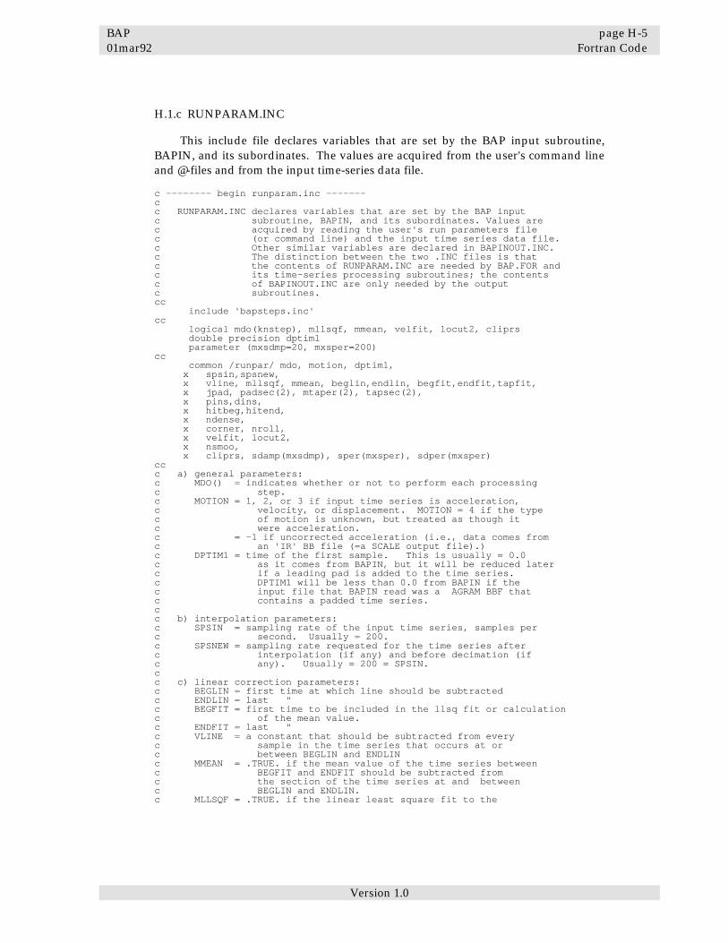
BAP page H-5 01mar92 Fortran Code
Version 1.0
H.1.c RUNPARAM.INC This include file declares variables that are set by the BAP input subroutine, BAPIN, and its subordinates. The values are acquired from the user's command line and @-files and from the input time-series data file. c -------- begin runparam.inc ------- c c RUNPARAM.INC declares variables that are set by the BAP input c subroutine, BAPIN, and its subordinates. Values are c acquired by reading the user's run parameters file c (or command line) and the input time series data file. c Other similar variables are declared in BAPINOUT.INC. c The distinction between the two .INC files is that c the contents of RUNPARAM.INC are needed by BAP.FOR and c its time-series processing subroutines; the contents c of BAPINOUT.INC are only needed by the output c subroutines. cc include 'bapsteps.inc' cc logical mdo(knstep), mllsqf, mmean, velfit, locut2, cliprs double precision dptim1 parameter (mxsdmp=20, mxsper=200) cc common /runpar/ mdo, motion, dptim1, x spsin,spsnew, x vline, mllsqf, mmean, beglin,endlin, begfit,endfit,tapfit, x jpad, padsec(2), mtaper(2), tapsec(2), x pins,dins, x hitbeg,hitend, x ndense, x corner, nroll, x velfit, locut2, x nsmoo, x cliprs, sdamp(mxsdmp), sper(mxsper), sdper(mxsper) cc c a) general parameters: c MDO() = indicates whether or not to perform each processing c step. c MOTION = 1, 2, or 3 if input time series is acceleration, c velocity, or displacement. MOTION = 4 if the type c of motion is unknown, but treated as though it c were acceleration. c = -1 if uncorrected acceleration (i.e., data comes from c an 'IR' BB file (=a SCALE output file).) c DPTIM1 = time of the first sample. This is usually = 0.0 c as it comes from BAPIN, but it will be reduced later c if a leading pad is added to the time series. c DPTIM1 will be less than 0.0 from BAPIN if the c input file that BAPIN read was a AGRAM BBF that c contains a padded time series. c c b) interpolation parameters: c SPSIN = sampling rate of the input time series, samples per c second. Usually = 200. c SPSNEW = sampling rate requested for the time series after c interpolation (if any) and before decimation (if c any). Usually = 200 = SPSIN. c c c) linear correction parameters: c BEGLIN = first time at which line should be subtracted c ENDLIN = last " c BEGFIT = first time to be included in the llsq fit or calculation c of the mean value. c ENDFIT = last " c VLINE = a constant that should be subtracted from every c sample in the time series that occurs at or c between BEGLIN and ENDLIN c MMEAN = .TRUE. if the mean value of the time series between c BEGFIT and ENDFIT should be subtracted from c the section of the time series at and between c BEGLIN and ENDLIN. c MLLSQF = .TRUE. if the linear least square fit to the

page H-6 BAP Fortran Code 01mar92
Version 1.0
c time series between BEGFIT and ENDFIT should c be subtracted from the section of the time series c at and between BEGLIN and ENDLIN. c c d) padding parameters: c PADSEC(1 & 2) = length of the leading and trailing pad c areas, in seconds. c MTAPER(1 & 2) = tapering option, one for each end of the c time series. Usually = 0. c = 0=> notaper, c = 1=> zcross, c = 2=> datataper, c TAPSEC(1 & 2) = taper length used with the datataper option. c Given as number of seconds in the taper. c Usually= 0.2. c c e) instrument correction parameters: c PINS = period of the recording transducer, in seconds, c usually about 0.06. c DINS = damping of the recording transducer, fraction of c critical damping, usually about 0.6. c c f) high-cut filter parameters; c HICUTT, HICUTZ = the transition band, in Hz, for the hi-cut c filter that is applied along with the instrument c correction. HICUTT is usually 50 and is the c frequency at which the cosine taper begins: the end c of the pass band. HICUTZ is usually 100 and is the c frequency at which the cosine taper ends: the c beginning of the stop band. c c g) decimation parameters: c NDENSE = ratio of the dense sample rate to the final sample c rate. The decimation step removes NDENSE-1 of c every NDENSE samples. Default NDENSE = 3. c c h) low-cut filter parameters: c CORNER = corner frequency for the low-cut, bi-pass Butterworth c filter. c MROLL = roll-off parameter for the low-cut, bi-pass Butterworth c filter. c c i) FAS parameters: c NSMOO = *** c c j) RSPEC parameters: c SDAMP()= *** c SPER () c SDPER() c c k) debug/test/development parameters: c JPAD,LOCUT2, CLIPRS c -------- end of runparam.inc ------- H.1.d BAPUNITS.INC This include file declares the common that will contain the names and units of the three types of time series that are manipulated by BAP: acceleration, velocity and displacement. c -------- begin bapunits.inc ------- c c BAPUNITS.INC declares /UNITS/, the common that contains the names c and units of the 3 types of time series that are c manipulated by BAP: acceleration, velocity and c displacement. The contents of /UNITS/ is assigned c in subroutine BAPDEF. cc character*(12) csname(4) character*(10) csunit(4) common /units/ csname, csunit c -------- end of bapunits.inc -------

BAP page H-7 01mar92 Fortran Code
Version 1.0
H.1.e TEMPCS.INC This include file declares space used for temporary character strings. c ---- begin TEMPCS.INC --- c c TEMPCS.INC declares /TEMPCS/ the common used for a temporary c character string. We're putting this in a common c just so it can be shared, avoiding the need for c everyone to declare their own temporary character c string. cc character*132 tempcs common /tempcs/ tempcs c ---- end TEMPCS.INC --- H.1.f FILNAM.INC This include file allocates character space used for constructing a file names. It also defines symbolic constants that are machine-dependent and are related to the file naming conventions used on the relevant computer. c --- begin filnam.inc --- c FILNAM.INC, VAX version. c FILNAM.INC defines symbolic constants that are machine-dependent and c are related to the file names. c c YNAMF = maximum number of characters in a file name. c VEROKC= .true. if it is OK to have version fields in the file name. c LCLDIR= characters that represent the local working directory when c appearing in a file name. = '[]' on the VAXes. c SCRFIL= characters that indicate the name and location of a file c the various AGRAM programs can use as a temporary scratch file. c c FILNAM.INC also allocates space in /CFILNM/. It contains: c FILNAM = Character space used for constructing a file name. cc integer YNAMF parameter (YNAMF=128) logical verokc parameter (verokc = .true.) character*2 lcldir parameter (lcldir = '[]') character*17 scrfil parameter (scrfil = 'scr:agramjunk.tmp') cc character*128 filnam common /cfilnm/ filnam c --- end of filnam.inc ---

page H-8 BAP Fortran Code 01mar92
Version 1.0
H.2 BAP2.FOR Coordinates all the time-series processing functions. BAP2 is called from BAP (the "main" subroutine) to keep the time-series processing functions, which are handled in BAP2, separate from the overhead and input functions, which are handled in BAP. subroutine BAP2 (fmtin,lunusr,lunmsg,lundsk,lundin,luntmp,lundot, x workA, x workB, x workC, lenwrk, nwork,inpadl,inpadt) character*3 fmtin real workA(lenwrk), workB(lenwrk), workC(lenwrk) cc c BAP2 is called from BAP to co-ordinate the time-series processing c functions separate from the overhead and input functions, c which are performed in BAP. cc c On entry -- c FMTIN = format of the input time-series data file. c = 'BBF' or 'SMC'. c LUNUSR,LUNMSG,LUNDSK,LUNDIN,LUNTMP,LUNDOT c = logical unit numbers. See comments in BAP.FOR. c WORKA() = array containing the input time series. c WORKB() = empty array available for work space. c WORKC() = " c LENWRK = length of WORKA, B, & C. c NWORK = the number of time-series values in WORKA(). This c is the number of samples if we are dealing with c evenly-sampled data, or 2* the number of samples c if we are dealing with unevenly-sampled data. c INPADL = number of leading pad samples in the input time c series. INPADL usually = 0. c INPADT = number of trailing pad samples in the input time c series. INPADT usually = 0. c c And the commons declared in RUNPARAM.INC have been filled with c run parameters acquired from the users command line and the c input time-series data file. See comments in the RUNPARAM.INC c file for description of each variable therein. cc c Commons and symbolic constants: cc include 'runparam.inc/nolist' include 'bapconst.inc/nolist' include 'tempcs.inc/nolist' include 'filnam.inc/nolist' ! *** will tempcs do? cc c Time calculations often will be done in double precison: cc double precision dpdelt, dpv, dpd, hdt double precision dpvlst, dp cc c Miscellaneous local variables: cc character*1 onec logical opened, skip, dbgz, doit, tfjunk parameter (dbgz=.false.) cc c SPS and DPDELT = current samples-per-second and sampling-interval. cc sps = spsin if (sps .gt. small) then dpdelt = dble(1.0)/dble(sps) else dpdelt = 0.0 endif cc c Plot and/or rewrite the input time series, if requested. cc write (lunmsg, 1401) fmtin if (lunusr.ne.lunmsg) write (lunusr, 1401) fmtin call BAPOUT (kinput, motion, lunmsg,lunusr,lundot,lundin,
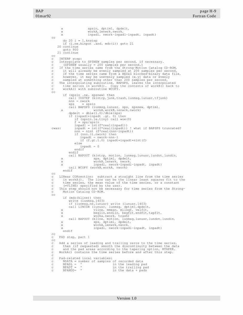
BAP page H-9 01mar92 Fortran Code
Version 1.0
x spsin, dptim1, dpdelt, x workA,lenwrk,nwork, x inpadl, nwork-inpadl-inpadt, inpadt) cc do 20 i = 1,knstep if (i.ne.kinput .and. mdo(i)) goto 21 20 continue goto 900 21 continue cc c INTERP step: c Interpolate to SPSNEW samples per second, if necessary. c (SPSNEW usually = 200 samples per second.) c If the time series came from the Strong-Motion Catalog CD-ROM, c it will already be evenly sampled at 200 samples per second. c If the time series came from a BES&G blocked-binary data file, c however, it may be unevenly sampled (x,y) data or evenly c sampled at something other than 200 samples per second. c The interpolating subroutine, BAPSPS, leaves the interpolated c time series in workB(). Copy the contents of workB() back to c workA() with subroutine WCOPY. cc if (spsin .ne. spsnew) then call IDSTEP (kintrp,junk,trash,lunmsg,lunusr,tfjunk) nnn = nwork sps = spsin call BAPSPS (lunmsg,lunusr, sps, spsnew, dptim1, x workA,workB,lenwrk,nwork) dpdelt = dble(1.0)/dble(sps) if (inpadl+inpadt .gt. 0) then if (spsin.le.tiny) call woe(0) f = sps/spsin inpadl = int(f*real(inpadl)) cwas: inpadt = int(f*real(inpadt)) ! what if BAPSPS truncated? nnn = nint (f*real(nnn-inpadt)) if (nnn.lt.nwork) then inpadt = nwork-nnn-1 if (f.gt.1.0) inpadt=inpadt+nint(f) else inpadt = 0 endif endif call BAPOUT (kintrp, motion, lunmsg,lunusr,lundot,lundin, x sps, dptim1, dpdelt, x workB,lenwrk, nwork, x inpadl, nwork-inpadl-inpadt, inpadt) call WCOPY (workB,workA, nwork) endif cc c LINear CORrection: subtract a straight line from the time series c in workA(). The line can be the linear least squares fit to the c time series, the mean value of the time series, or a constant c (=VLINE) specified by the user. c This step should not be necessary for time series from the Strong- c Motion Catalog CD-ROM. cc if (mdo(kline)) then write (lunmsg,1403) if (lunmsg.ne.lunusr) write (lunusr,1403) call LINCOR (lunusr, lunmsg, dptim1,dpdelt, x vline, mmean, mllsqf, velfit, x beglin,endlin, begfit,endfit,tapfit, x worka,nwork, trash) call BAPOUT (kline, motion, lunmsg,lunusr,lundot,lundin, x sps, dptim1, dpdelt, x workA,lenwrk,nwork, x inpadl, nwork-inpadl-inpadt, inpadt) endif cc c PAD step, part 1 cc c Add a series of leading and trailing zeros to the time series, c then (if requested) smooth the discontinuity between the data c and the pad areas according to the tapering option, MTAPER. c WorkA() contains the time series before and after this step. c c Pad-related local variables: c NDATA = number of samples of recorded data c NPADL = " in the leading pad c NPADT = " in the trailing pad c NPANDD= " in the data + pads
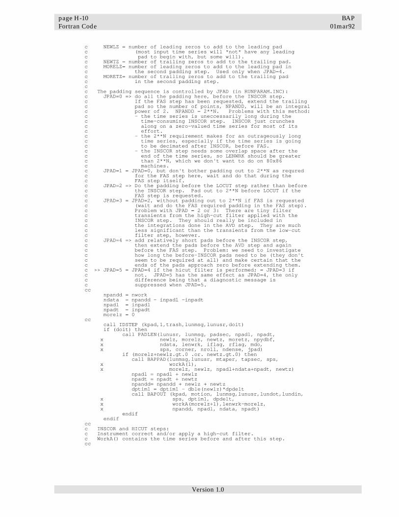
page H-10 BAP Fortran Code 01mar92
Version 1.0
c NEWLZ = number of leading zeros to add to the leading pad c (most input time series will *not* have any leading c pad to begin with, but some will). c NEWTZ = number of trailing zeros to add to the trailing pad. c MORELZ= number of leading zeros to add to the leading pad in c the second padding step. Used only when JPAD=4. c MORETZ= number of trailing zeros to add to the trailing pad c in the second padding step. c c The padding sequence is controlled by JPAD (in RUNPARAM.INC): c JPAD=0 => do all the padding here, before the INSCOR step. c If the FAS step has been requested, extend the trailing c pad so the number of points, NPANDD, will be an integral c power of 2. NPANDD = 2**N. Problems with this method: c - the time series is uneccessarily long during the c time-consuming INSCOR step. INSCOR just crunches c along on a zero-valued time series for most of its c effort. c - the 2**N requirement makes for an outrageously long c time series, especially if the time series is going c to be decimated after INSCOR, before FAS. c - the INSCOR step needs some overlap space after the c end of the time series, so LENWRK should be greater c than 2**N, which we don't want to do on 80x86 c machines. c JPAD=1 = JPAD=0, but don't bother padding out to 2**N as requred c for the FAS step here, wait and do that during the c FAS step itself. c JPAD=2 => Do the padding before the LOCUT step rather than before c the INSCOR step. Pad out to 2**N before LOCUT if the c FAS step is requested. c JPAD=3 = JPAD=2, without padding out to 2**N if FAS is requested c (wait and do the FAS required padding in the FAS step). c Problem with JPAD = 2 or 3: There are tiny filter c transients from the high-cut filter applied with the c INSCOR step. They should really be included in c the integrations done in the AVD step. They are much c less significant than the transients from the low-cut c filter step, however. c JPAD=4 => add relatively short pads before the INSCOR step, c then extend the pads before the AVD step and again c before the FAS step. Problem: we need to investigate c how long the before-INSCOR pads need to be (they don't c seem to be required at all) and make certain that the c ends of the pads approach zero before extending them. c >> JPAD=5 = JPAD=4 if the hicut filter is performed; = JPAD=3 if c not. JPAD=5 has the same effect as JPAD=4, the only c difference being that a diagnostic message is c suppressed when JPAD=5. cc npandd = nwork ndata = npandd - inpadl -inpadt npadl = inpadl npadt = inpadt morelz = 0 cc call IDSTEP (kpad,1,trash,lunmsg,lunusr,doit) if (doit) then call PADLEN(lunusr, lunmsg, padsec, npadl, npadt, x newlz, morelz, newtz, moretz, npydbf, x ndata, lenwrk, iflag, rflag, mdo, x sps, corner, nroll, ndense, jpad) if (morelz+newlz.gt.0 .or. newtz.gt.0) then call BAPPAD(lunmsg,lunusr, mtaper, tapsec, sps, x workA(1), x morelz, newlz, npadl+ndata+npadt, newtz) npadl = npadl + newlz npadt = npadt + newtz npandd= npandd + newlz + newtz dptim1 = dptim1 - dble(newlz)*dpdelt call BAPOUT (kpad, motion, lunmsg,lunusr,lundot,lundin, x sps, dptim1, dpdelt, x workA(morelz+1),lenwrk-morelz, x npandd, npadl, ndata, npadt) endif endif cc c INSCOR and HICUT steps: c Instrument correct and/or apply a high-cut filter. c WorkA() contains the time series before and after this step. cc

BAP page H-11 01mar92 Fortran Code
Version 1.0
call IDSTEP (kinsc,nowstp,trash,lunmsg,lunusr,doit) if (doit) then ndone = -1 call FDIC(lunmsg,lunusr,workA(morelz+1),npandd,ndone, x lenwrk-morelz, x dpdelt, mdo(kinsc), pins,dins,hitbeg,hitend) if (motion.lt.0) motion = -motion if (dbgz) call SHOWZ (npadl,ndata,npadt,workA(morelz+1),npandd) if (jpad.eq.0 .and. ndone.lt.npandd .and. ndone.gt.npydbf) then do 140 i = morelz+ndone+1, morelz+npandd workA(i)=0.0 140 continue ndone = npandd endif if (ndone.lt.npandd) then write (lunmsg, 2001) npandd, ndone, lenwrk if (lunmsg.ne.lunusr) write (lunusr, 2001) x npandd, ndone, lenwrk npandd = ndone if (ndone.gt.npadl+ndata) then npadt = ndone -npadl-ndata else if(ndone.gt.npadl) then npadt = 0 ndata = ndone -npadl endif endif call BAPOUT (nowstp, motion, lunmsg,lunusr,lundot,lundin, x sps, dptim1, dpdelt, x workA(morelz+1),lenwrk-morelz, x npandd, npadl,ndata,npadt) endif cc c DECIMation: reduce the sampling rate by removing NDENSE-1 c of every NDENSE samples. c WorkA() contains the time series before and after this step. cc if (mdo(kdecim) .and. ndense.gt.1) then dp = sps dp = dp/dble(ndense) call IDSTEP (kdecim,junk,sngl(dp),lunmsg,lunusr,doit) if (doit) then sps=sngl (dp) dpdelt = dble(1.0)/dp cc n = npadl/ndense n = npadl - n*ndense j = morelz do 110 i = morelz+1+n, morelz+npandd, ndense j = j+1 workA(j) = workA(i) 110 continue cc npandd = j - morelz npadl = npadl/ndense ndata = (ndata+ndense-1)/ndense npadt = npandd-npadl-ndata cc call BAPOUT (kdecim, motion, lunmsg,lunusr,lundot,lundin, x sps, dptim1, dpdelt, x workA(morelz+1), lenwrk-morelz, x npandd, npadl,ndata,npadt) endif endif cc c PAD step, part 2 c WorkA() contains the time series before and after this step. cc call IDSTEP (kpad,2,trash,lunusr,lunmsg,doit) if (doit) then if (jpad.eq.4) then if (morelz+npandd+moretz.gt.lenwrk) x moretz = max(0,lenwrk -npandd-morelz) newlz =morelz newtz =moretz call BAPPD2(lunusr,lunmsg, x workA, morelz,npadl,ndata,npadt,moretz) else call PADLEN(lunusr,lunmsg, padsec, npadl, npadt, x newlz, junk, newtz, junk2, junk3, x ndata, lenwrk, iflag, rflag, mdo, x sps, corner, nroll, 1, jpad)

page H-12 BAP Fortran Code 01mar92
Version 1.0
if (newlz.gt.0 .or. newtz.gt.0) then call BAPPAD(lunusr,lunmsg, mtaper, tapsec,sps, x workA, x 0, newlz, npadl+ndata+npadt, newtz) endif endif if (newlz.gt.0 .or. newtz.gt.0) then npadl = npadl + newlz npadt = npadt + newtz npandd= npandd + newlz + newtz dptim1 = dptim1 - dble(newlz)*dpdelt call BAPOUT (kpad, motion, lunmsg,lunusr,lundot,lundin, x sps, dptim1, dpdelt, x workA,lenwrk, npandd, npadl, ndata, npadt) endif endif cc c AVD step, LOCUT2 version: integrate acceleration to velocity c before the acceleration is filtered; filter velocity; integrate c velocity to displacement. c WorkB() contains the new velocity time series after this step and c WorkC() contains the new displacement time series. c Write velocity and displacement. cc call IDSTEP (kavd, 0,trash,lunmsg,lunusr,doit) if (doit) then hdt = dpdelt*dble(0.5) dpv =0.0 alast=0.0 do 126 i = 1, npandd dpv = dpv + (workA(i) + alast) *hdt alast = workA(i) workB(i)= sngl(dpv) 126 continue call BIhip(workB,npandd,dble(corner),dpdelt,nroll) call BAPOUT (kavd, 2, lunmsg,lunusr,lundot,lundin, x sps, dptim1, dpdelt, x workB,lenwrk, npandd, npadl, ndata, npadt) cc vlast = 0.0 dpd = 0.0 do 124 i = 1, npandd vel = workB(i) dpd = dpd + dble(vel + vlast)*hdt workC(i) = sngl(dpd) vlast = vel 124 continue call BAPOUT (kavd, 3, lunmsg,lunusr,lundot,lundin, x sps, dptim1, dpdelt, x workC,lenwrk, npandd, npadl, ndata, npadt) endif cc c LOCUT step: remove long period content with a bidirectional, c high-pass (=low-cut) Butterworth filter. c WorkA() contains the time series before and after this step. cc call IDSTEP (klocut,junk,trash,lunmsg,lunusr,doit) if (doit) then call BIHIP (workA,npandd,dble(corner),dpdelt,nroll) call BAPOUT (klocut, motion, lunmsg,lunusr,lundot,lundin, x sps, dptim1, dpdelt, x workA,lenwrk, npandd, npadl, ndata, npadt) if (dbgz) call SHOWZ (npadl,ndata,npadt, workA, npandd) endif cc c AVD step, standard version (locut2=.false.): c If input time series is acceleration, integrate acceleration c to calculate velocity. If the VELFIT option is requested, c subtract the linear-least-squares fit of the velocity from c the velocity and subtract the slope of that line from the c acceleration. c Or, if the input time series is velocity, differentiate to c calculate acceleration. c In either case, once we have a velocity time series, integrate c that to calculate displacement. c Include the pad areas in the integration bounds. c After this step, workA() contains acceleration, c workB() contains velocity, and c workC() contains displacement. cc if (.not. locut2) then
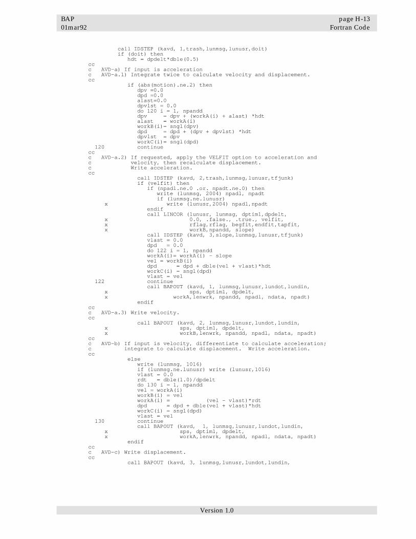
BAP page H-13 01mar92 Fortran Code
Version 1.0
call IDSTEP (kavd, 1,trash,lunmsg,lunusr,doit) if (doit) then hdt = dpdelt*dble(0.5) cc c AVD-a) If input is acceleration c AVD-a.1) Integrate twice to calculate velocity and displacement. cc if (abs(motion).ne.2) then dpv =0.0 dpd =0.0 alast=0.0 dpvlst = 0.0 do 120 i = 1, npandd dpv = dpv + (workA(i) + alast) *hdt alast = workA(i) workB(i)= sngl(dpv) dpd = dpd + (dpv + dpvlst) *hdt dpvlst = dpv workC(i)= sngl(dpd) 120 continue cc c AVD-a.2) If requested, apply the VELFIT option to acceleration and c velocity, then recalculate displacement. c Write acceleration. cc call IDSTEP (kavd, 2,trash,lunmsg,lunusr,tfjunk) if (velfit) then if (npadl.ne.0 .or. npadt.ne.0) then write (lunmsg, 2004) npadl, npadt if (lunmsg.ne.lunusr) x write (lunusr,2004) npadl,npadt endif call LINCOR (lunusr, lunmsg, dptim1,dpdelt, x 0.0, .false., .true., velfit, x rflag,rflag, begfit,endfit,tapfit, x workB,npandd, slope) call IDSTEP (kavd, 3,slope,lunmsg,lunusr,tfjunk) vlast = 0.0 dpd = 0.0 do 122 i = 1, npandd workA(i)= workA(i) - slope vel = workB(i) dpd = dpd + dble(vel + vlast)*hdt workC(i) = sngl(dpd) vlast = vel 122 continue call BAPOUT (kavd, 1, lunmsg,lunusr,lundot,lundin, x sps, dptim1, dpdelt, x workA,lenwrk, npandd, npadl, ndata, npadt) endif cc c AVD-a.3) Write velocity. cc call BAPOUT (kavd, 2, lunmsg,lunusr,lundot,lundin, x sps, dptim1, dpdelt, x workB,lenwrk, npandd, npadl, ndata, npadt) cc c AVD-b) If input is velocity, differentiate to calculate acceleration; c integrate to calculate displacement. Write acceleration. cc else write (lunmsg, 1016) if (lunmsg.ne.lunusr) write (lunusr,1016) vlast = 0.0 rdt = dble(1.0)/dpdelt do 130 i = 1, npandd vel = workA(i) workB(i) = vel workA(i) = (vel - vlast)*rdt dpd = dpd + dble(vel + vlast)*hdt workC(i) = sngl(dpd) vlast = vel 130 continue call BAPOUT (kavd, 1, lunmsg,lunusr,lundot,lundin, x sps, dptim1, dpdelt, x workA,lenwrk, npandd, npadl, ndata, npadt) endif cc c AVD-c) Write displacement. cc call BAPOUT (kavd, 3, lunmsg,lunusr,lundot,lundin,

page H-14 BAP Fortran Code 01mar92
Version 1.0
x sps, dptim1, dpdelt, x workC,lenwrk, npandd, npadl, ndata, npadt) endif endif cc c FAS step: c Calculate and plot the Fourier amplitude spectrum. c BAPFAS replaces the time series it is given, so copy the c contents of WorkA(), where the acceleration is now, to c WorkB() and pass the WorkB() copy to BAPFAS. cc if (mdo(kfas)) then write (lunmsg, 1410) if (lunmsg.ne.lunusr) write (lunusr,1410) call WCOPY (workA,workB, npandd) lunfas=0 call BAPC (lunmsg,lunusr,kfas,1,luntmp, x opened, filnam,onec) if (opened) lunfas=luntmp call BAPFAS(lunmsg, lunusr, lunfas, x nsmoo, motion, dpdelt, x workB,lenwrk,npandd, nf,deltaf) n=lnbc1(filnam) call BAPFAP (lunmsg, lunusr, nsmoo, workB,nf,deltaf, x kfas,1,filnam(1:n)) if (lunfas.ne.0) then close(unit=lunfas) n = min( 130-11, n) write (lunmsg, 1008) filnam(1:n) if (lunmsg.ne.lunusr) write (lunusr,1008) filnam(1:n) endif endif cc c RSPEC step: Calculate and plot response spectra. c BAPRSI (initialization) sets the period and damping lists. c BAPRSC calculates a response spectrum for each damping value. c BAPRSP plots the response spectra. c The acceleration time series is in workA(), so we can use workB() c and workC() for work space: c workC(1 thru NPER )= list of period values assigned in BAPRSI. c There will be NPER points in each curve (or c spectrum) plotted by BAPRSP, one for each c period value. c workC(1+NPER ...) is used as the PRV(j,k) array in BAPRSC and c BAPRSP. It receives the maximum pseudo- c velocity response calculated by BAPRSC for c the j-th period, k-th damping. c workB() is used as the RV(j,k) array in BAPRSC and c BAPRSP. It receives the maximum relative c velocity response calculated by BAPRSC for c the j-th period, k-th damping. c c SDAMP(1 thru NDAMP)= list of user-specified damping values. c There will be NDAMP curves on each plot page c generated in BAPRSP, one curve for each c damping value. cc if (mdo(kresp)) then write (lunmsg, 1411) if (lunmsg.ne.lunusr) write (lunusr,1411) call BAPRSI(lunmsg, lunusr, rflag, sper, sdper, mxsper, x workC, nper, lenwrk, sdamp, ndamp, mxsdmp, skip) if (.not. skip) then locprv = 1 + nper if (locprv + nper*ndamp .gt. lenwrk) call woe(0) lunres=0 call BAPC (lunmsg,lunusr,kresp,1,luntmp, x opened, filnam,onec) if (opened) lunres=luntmp call BAPRSC(lunmsg,lunusr,lunres,sngl(dpdelt),workA,npandd, x sdamp, ndamp, workC, nper, x workB, workC(locprv) ) if (lunres.ne.0) then close(unit=lunres) n = min (130-11, lnbc1(filnam)) write (lunmsg, 1009) filnam(1:n) if (lunmsg.ne.lunusr) write (lunusr,1009) filnam(1:n) endif call BAPRSP(sdamp, ndamp, workC, nper, x workB, workC(locprv), sps, cliprs, x lunmsg,lunusr,kresp,1,filnam(1:lnbc1(filnam)))

BAP page H-15 01mar92 Fortran Code
Version 1.0
endif endif cc c Done. cc 900 continue return cc 3000 format (' ') cc 1401 format (/5x, 'INPUT time series (input format = ',a,')' x /5x, '=================' x/8x, 'Characteristics of the input time series:') 1403 format (/5x, 'LINear CORrection step' x /5x, '======================') 1410 format (/5x, 'FAS step' /5x, '========' x/8x,'Calculate Fourier amplitude spectrum of acceleration.') 1411 format(/5x, 'RESPON step', /5x, '==========' x/8x,'Calculate response spectra from the acceleration' x, ' time series.' ) 1412 format(/5x, 'DONE.', /5x, '=====') 1413 format (8x, x'A copy of all the run messages shown here on the screen have' x/8x,'been saved in the disk file at: ', a) 1414 format (8x, x'A copy of all the run messages shown here on the screen have' x/8x,'been saved in the disk file at: ' x/8x, a) cc 1016 format (5x, x'Differentiate the time series (=velocity) to calculate' x/8x,'acceleration, integrate to calculate displacement.') 1008 format(8x, x'Output Fourier amplitude file format = BAP text, file name = ' x/11x, a) 1009 format(8x, x'Output response spectra file format = BAP text, file name = ' x/11x, a) 1020 format(/5x,'No plots were generated in this BAP run.') cc 2001 format(/3x, x' *** WARNING: the padded time series has been truncated from',i8, x/8x, 'samples to', i8, ' samples due to lack of space in the' x/8x,'working array (length =',i8, ') during instrument correction' x/8x,'calculations. ***' /) 2004 format(/' *** ',3x, x 'WARNING: the VELFIT option should usually not be used on a' x/11x, 'PADded time series. (npadl=',i8 x, ' npadt=,'i8,') ***' /) cccccccccccccccccccc (end of BAP2/BAP)cccccccccccccccccccccccccccccccccc end c subroutine WCOPY(work1,work2,npoint) real work1(npoint), work2(npoint) cc c WCOPY is called from BAP2 to copy the contents of WORK1() c into WORK2(). cc do 100 i =1,npoint work2(i)=work1(i) 100 continue return cccccccccccccccccccc (end of WCOPY/BAP2/BAP) ccccccccccccccccccccccccccc end

page H-16 BAP Fortran Code 01mar92
Version 1.0
H.3 BAPSPS.FOR Subroutine BAPSPS linearly interpolates the time series to a new sampling interval. subroutine bapsps (lunusr, lunmsg, sps, spsnew, dptim1, x workA,workB,lenwrk,nwork) double precision dptim1 real workA(lenwrk), workB(lenwrk) cc c BAPSPS: Linearly interpolate the BAP input time series to SPSNEW c samples per second. c Note that this subroutine does *not* apply any high-cut c filter to remove alias errors. c c On entry-- c SPS = input sample rate if WORKA() contains an evenly sampled c series of y-values, or c = 0.0 to indicate that the input time series is a series c of unevenly sampled (x,y) pairs. c SPSNEW = requested new sample rate, usually = 200. c (SPSNEW must not = SPS, for this subroutine assumes c that it would not have been called if that were the c case.) c DPTIM1 = time of the first sample (almost always = 0.0) c >>> Note that this is in double precision. c WORKA() = input time series. c NWORK = number of values in WORKA(). c LENWRK = maximun length (= dimension) of WORKA() and of WORKB(). c c On return -- c SPS = SPSNEW = output sample rate c WORKB() = output time series c NWORK = number of evenly-sampled points in WORKB() cc include 'bapconst.inc' double precision time, timea, timeb, dtold, dtnew cc if (small .gt. spsnew) call woe(0) if (small .gt. abs(spsnew-sps)) call woe(0) cc dtnew = dble(1.0)/dble(spsnew) nin = nwork smidge = small*dtnew if (sps .le. 0.0) then if (sngl(dptim1).ne.workA(1)) call woe(0) yb = workA(2) istep= 2 else dtold = dble(1.0)/dble(sps) yb = workA(1) istep= 1 endif workB(1) = yb timeb = dptim1 time = dptim1 + dtnew nwork = 1 do 30 i = istep+1, nin, istep timea = timeb ya = yb if (istep.eq.1) then timeb = dptim1 + dtold*dble(i-1) yb = workA(i) else timeb = workA(i) yb = workA(i+1) endif cc 40 continue if (timeb. le.timea + smidge) then goto 30 else if (time .lt. timea) then call woe(0) elseif (time.ge. timea .and. time.le.timeb) then nwork = nwork + 1

BAP page H-17 01mar92 Fortran Code
Version 1.0
if (nwork.gt.lenwrk) then nwork = nwork-1 write (lunmsg,1003) sngl(time), lenwrk if (lunmsg.ne.lunusr) x write (lunmsg,1003) sngl(time), lenwrk call warn ('*',lunusr,lunmsg) go to 31 endif workB(nwork) x = ya + (yb-ya)*((time - timea)/(timeb-timea)) time = dptim1 + dtnew*dble(nwork) go to 40 endif 30 continue 31 continue sps = spsnew return cc 1003 format (/' *** Truncating time series at ', e13.5,' seconds, due' x/5x,'to insufficient space in the working array. Length of the' x/5x,'working array =', i8, '. ***' /) cccccccccccccccccccc (end of BAPSPS) ccccccccccccccccccccccccccccccccccc end

page H-18 BAP Fortran Code 01mar92
Version 1.0
H.4 BAPPAD.FOR Subroutine BAPPAD adds zero-padding before and after the time series and, if requested, applies a tapering option to the discontinuity between the data and the pad. subroutine BAPPAD(lunusr,lunmsg, x mtaper,tapsec, sps,work, x morelz,newlz,ndata,newtz, doit2) real work(morelz+newlz+ndata+newtz) real tapsec(2) integer mtaper(2) logical doit2 cc c BAPPAD pads the time series in WORK() with leading and trailing c zeros, then smooths the discontinuity between the data and c the pad areas according to the tapering option, MTAPER. c c On entry -- c LUNMSG = lun for run messages = user's terminal or disk file. c LUNUSR = " = user's terminal. c MTAPER() = tapering option, one for each end of the time-series: c = 0=> notaper; c = 1=> zcross = reset to zero all values for samples c that occur before the first zero c crossing or after the last zero c crossing; c = 2=> datataper = apply a cosine taper at the end of c the time series. c TAPSEC() = taper length used with the datataper option, in c seconds. TAPSEC indicates the number of points to c be used in the taper, excluding the endpoints at c taper-factor = 0.0 and at taper-factor = 1.0. c SPS = sampling rate c WORK() = array containing a time-series plus free space for c padding. The unpadded input time series is in c locations 1 thru NDATA. c MORELZ = empty space to be left at the beginning of the padded c time series. (Will be used in the second padding c step) c NEWLZ = number of zeros requested for the leading pad. c NDATA = number of samples (beginning at WORK(1)) in the c input time series. c NEWTZ = number of zeros requested for the trailing pad. c c NOTES: c - Before calling BAPPAD, the caller must make certain that c there is enough space in WORK() to contain NEWLZ+NDATA+NEWTZ c samples. c - NEWLZ and NEWTZ may =0 if tapering is wanted, without the c padding. (As might be appropriate when VELFIT=.true.) c c On return -- c WORK() = contains the padded time series in locations MORELZ +1 c thru MORELZ + newlz + NDATA + newtz. c DOIT2 = .false. if there really wasn't any padding or tapering c applied to the time series. cc include 'bapconst.inc' include 'tempcs.inc' parameter (pi =3.1415926535) real ntaper(2) logical shift cc lztot = newlz+morelz doit2 = .true. if (newlz.eq.0 .and. newtz.eq.0) then write (lunmsg,1000) if (lunusr.ne.lunmsg) write (lunusr,1000) if (mtaper(1).le.0 .and. mtaper(2).le.0) then doit2 = .false. if (morelz.le.0) return endif endif

BAP page H-19 01mar92 Fortran Code
Version 1.0
cc ntaper(1) = max(0, nint(tapsec(1)*sps) -2) ntaper(2) = max(0, nint(tapsec(2)*sps) -2) cc data1 = work(1) datan = work(ndata) idata1 = lztot + 1 idatan = lztot + ndata cc c Shift the time series forward in WORK(), to leave room for the c leading pad. cc shift = .true. if (lztot.le.0) shift=.false. smidge = 0.0 do 120 i = idatan,idata1, -1 if (shift) work(i) = work(i-lztot) if (abs(work(i)) .gt. smidge) smidge = abs(work(i)) 120 continue if (.not. doit2) return smidge = small*smidge cc c If the "ZCROSS" taper option was specified, find the first and last c zero-crossings in the time-series. cc izc1=-1 izcn=-1 if (mtaper(1).eq.1 .or. mtaper(2).eq.1) then if (abs(data1).lt.smidge) then izc1=idata1 else if (ndata.gt.2) then do 31 i=idata1+1, idatan-1 if (work(i)*data1.lt.0.0) then izc1=idata1 j=i if(abs(work(i-1)) .lt. abs(work(i))) j=i-1 if(abs(work(j)) .lt. abs(data1)) izc1=i go to 32 endif 31 continue 32 continue endif if (abs(datan).lt.smidge) then izcn=idatan elseif (ndata.gt.2 .and. izc1 .lt. idatan) then cwas: do 33 i= idatan-1, max(idata1+1,izc1), -1 do 33 i= idatan-1, max(idata1,izc1-1), -1 if (work(i)*datan.lt.0.0) then izcn=idatan j=i if(abs(work(i+1)) .lt. abs(work(i))) j=i+1 if(abs(work(j)) .lt. abs(datan)) izcn=i go to 34 endif 33 continue 34 continue endif if (izcn.le.izc1 .or. izc1.lt.0) then write(lunmsg,1101) if (lunusr.ne.lunmsg) write(lunusr,1101) call warn ('*',lunusr,lunmsg) if ((mtaper(1).eq.1 .and. mtaper(2).eq.1) .or. x (mtaper(1).eq.1 .and. izc1.eq.-1) .or. x (mtaper(2).eq.1 .and. izcn.eq.-1) ) then c +++ call woe(2) +++ do we want to continue here or croak? izc1 = idata1 izcn = idatan endif endif endif cc c Begin Loop to pad and taper each end of the time-series. cc do 500 ipad = 1,2 itap = mtaper(ipad) nzdata = 0 k2beg = 9 if (ipad.eq.1) then tempcs(1:8) = 'leading ' tempcs(9:13)= 'first' k2end = 13

page H-20 BAP Fortran Code 01mar92
Version 1.0
locbeg = 1 locend = lztot npad = newlz ilow = idata1 jdir = -1 if (itap.eq.1) then locend = izc1 -1 nzdata = locend - lztot endif else tempcs(1:8) = 'trailing' tempcs(9:12)= 'last' k2end = 12 locbeg = 1 + idatan locend = newtz + idatan npad = newtz ilow = idatan jdir = 1 if (itap.eq.1) then locbeg = izcn +1 nzdata = idatan -izcn endif endif cc c a) Pad with zeros and, if requested, extend the zeros into the c data area, up to the first zero crossing. cc if (locbeg.lt.locend) then do 10 i= locbeg,locend work(i)=0.0 10 continue write (lunmsg,1002) npad, tempcs(1:8) if (lunusr.ne.lunmsg) write (lunusr,1002) npad, tempcs(1:8) if (itap.eq.1 .and. nzdata.gt.0) then write (lunmsg,1030) tempcs(k2beg:k2end), nzdata if (lunusr.ne.lunmsg) write (lunusr,1030) x tempcs(k2beg:k2end), nzdata endif else write(lunmsg,1001) tempcs(1:8) if (lunusr.ne.lunmsg) write(lunusr,1001) tempcs(1:8) endif cc c b) If requested, apply a cosine taper at both ends of the data area. c (cos(0)=1.0; cos(pi/2) =0.0; cos(pi)=-1.0) c Apply the taper so the lowest point in the taper (0.0) falls at c the first point in the pad. c Note that NNN counts the number of interior points in the c taper, excluding the endpoints at F=1.0 and F=0.0. The c endpoint at f=1.0 is at sample number IHIGH, the endpoint c at f=0.0 is the first point in the pad. cc if (itap.eq.2) then nnn= ntaper(ipad) if (nnn.ge.1) then write(lunmsg,1010) tempcs(k2beg:k2end), nnn if (lunusr.ne.lunmsg) write(lunusr,1010) x tempcs(k2beg:k2end), nnn rstep = pi/float(nnn+1) ihigh = ilow -jdir*(nnn) do 101 j=1,nnn f = 0.5*(1.0+cos(rstep*float(j))) i = ihigh + j*jdir work(i) = work(i) * f 101 continue endif endif cc c End of loop. cc 500 continue return cc 1000 format(8x,'No padding requested (MORELZ+NEWLZ=NEWTZ=0).') 1001 format(8x, x'The time series has NOT been extended with ', a8, ' zeros.') 1002 format(8x, x'The time series has been extended with',i8, 1x, a8,' zeros.') 1010 format(11x, 'In addition, the ',a, i8, x' input samples were' x/11x,'weighted with a cosine taper so the sample values at the'

BAP page H-21 01mar92 Fortran Code
Version 1.0
x/11x,'end of the time-series approach zero.') 1030 format(11x, x'In addition, the ',a, i8 x,' input samples were reset' x,/11x, 'to zero.' ) 1101 format(/3x, x' *** The ZCROSS option should not be used with this data.' x/8x,'The time series does not contain two zero crossings! ***'/) cccccccccccccccccccc (end of BAPPAD) ccccccccccccccccccccccccccccccccccc end

page H-22 BAP Fortran Code 01mar92
Version 1.0
H.5 FDIC.FOR Subroutine FDIC applies instrument correction and/or a high-cut filter to the time series. subroutine fdic (lunusr,lunmsg, work,ndata,ndone,lenwrk,dpdelt, x minsc, pins,dins,hitbeg,hitend) real work(lenwrk) logical minsc double precision dpdelt cc c FDIC, 20feb92 version. c FDIC applies instrument correction and a high-cut filter to a c time series that represents response of a strong-motion c recording instrument. The time series is transformed to c the frequency domain, where the instrument correction and c filter are applied, then transformed back to the time domain. c FDIC is used in the HIFRIC program and in the BAP program. c c On entry -- c LUNMSG= lun for run messages = user's terminal or disk file. c LUNUSR= " = user's terminal. c WORK()= an array containing an equally-sampled instrument- c response time-series that has been scaled to c approximate ground acceleration but has not been c corrected for diminishing instrument reponse with c respect to increasing frequency. c NDATA = number of time-domain samples in WORK(). c If NDATA < LENWRK, then the excess space in WORK(), c beyond WORK(NDATA), will be filled with zeros. c NDONE = location of the last value in WORK() to have been c completely processed during a previous call to FDIC. c NDONE must= -1 in the first call to FDIC. c NDONE is used with repetitive calls to FDIC to process c a time series that will not fit in WORK(). Such c repetitive calls to FDIC are used in the HIFRIC c program, but not in the BAP program. NDONE will be c reset during each call to FDIC. After return from c FDIC, the caller may dispose of WORK(1 through NDONE), c shift the uncompleted time-series samples in WORK() to c the beginning of the array, reset NDONE, then add more c time series samples into the end of WORK() for c processing in a subsequent call to FDIC. c LENWRK= length of the array WORK(). c Want LENWRK .GE. N + an integral multiple of 1024, c (+ 2 if the ccFFT used here is replaced c with calls to FORK or RFFT) c where N = 0 in the first call to FDIC, c and N = NDONE + NLAP on subsequent calls. c (NLAP is defined below as 512, but may c change.) c DPDELT= time interval between the time-series samples in WORK(), c in seconds. Usually 1/200 when called from BAP; c 1/600 when called from HIFRIC. c >>> Note that DPDELT is in double precision. c MINSC = .FALSE. if instrument correction is not required, only c the high-cut filter. c PINS = period of the recording instrument, in seconds. c Usually about 0.05. c DINS = damping of the recording instrument, as fraction of c critical damping. Usually about 0.6 c HITBEG= Frequency, in Hz., at which the cosine taper in the c high-cut filter will begin. Usually = 50. c = end of the "pass band". c = beginning of the "transition band". c HITEND= frequency, in Hz., at which the cosine taper in the c high-cut filter will end. Usually = 100. c = beginning of the "stop band" c = end of the "transition band". c c On return -- c NDONE = location of the last sample in WORK() that was completely c processed during the current call to FDIC. c WORK(1 thru NDONE) c contains the instrument-corrected portion of the time
BAP page H-23 01mar92 Fortran Code
Version 1.0
c series. c WORK(NDONE+1 thru LENWRK) c contains partially corrected time series. c c c Authors c ======= c FDIC was originally written as subroutine INSCOR by William c Joyner at the USGS in Menlo Park. April Converse modified all but c the underlying technique in the process of adding all the comments, c run messages, and modifications that allow FDIC to be called c repeatedly (in the HIFRIC program) to process a large time series c that will not fit in the WORK() array. c c Warning c ======= c The NLAP value (see below) was selected as an interval much c longer than the time required for a corrected, filtered, single c pulse to decay to (close to) zero. If very different instrument or c filter characteristics are given than those that are normally c used (damping=0.6, period=0.05, sampling interval = 0.005, and c filter transition at 50 thru 100), the NLAP value may be too small. c Until more analysis and experiments are performed with this c algorithm, the input parameters should probably be restricted as c follows: c HITBEG <= HITEND - 2 (CDMG uses 23-25) c or preferably HITBEG <= 0.5*HITEND (USGS uses 50 to 100) c HITEND <= 0.5/DPDELT) c and PINS < 1.0 c c To experiment with these requirements, filter a unit pulse using c the desired values for PINS, DINS, DPDELT, HITBEG, and HITEND c with a large enough value for NTOT2 (it is defined below) that c the segmentation does not occur anywhere near the pulse. Plot c the results in short segments to see how large the filter c transients are at various intervals from the original pulse. c The SPIKE8.BBF file can be used as the input file; the TSPLOT c program can be used to plot the results. c c c Instrument correction c ===================== c The damped harmonic oscillator equation is used for instrument c correction. The instrument correcting equation in the time domain, c t, is: c c a(t) = x(t) + x'(t)*c + x''(t)*d [A] c c where a(t) = corrected acceleration sampled at equal intervals c (=DPDELT seconds) in time. c = the time series returned in WORK() from FDIC; c x(t) = instrument response scaled to approximate ground c acceleration. c = instrument response multiplied by a scale factor c proportional to (-u*u). c = the time series given in WORK() on entry to FDIC; c x'(t) = first derivative of x(t); c x''(t)= second derivative of x(t); c c = 2*DINS/u c d = 1.0/(u*u) c u = natural frequency of the recording instrument in c radians/sec c = 2*PI/PINS c PI = 3.14159 c PINS = instrument period, in seconds; c DINS = instrument damping as a fraction of critical damping; c and upper case words (like PI, PINS and DINS) are constant, c variable, or argument names used in the code. c c The equivalent instrument-correcting equation in the frequency c domain, f, is: c c b(f) = z(f) * (g + hi) [B] c c where z(f) = x(t) transformed via an FFT to an evenly-sampled c series in the frequency domain. z(f) is a series c of complex numbers, unlike x(t) which is a series c of real numbers. c b(f) = a(t) in the frequency domain. Like z(f), it is a c series of complex numbers. c (g + hi)= is a complex number having g as its real component, h

page H-24 BAP Fortran Code 01mar92
Version 1.0
c as its imaginary component, and: c g = 1.0 - (f*f * PINS*PINS) = FR c h = 2.0*f*DINS*PINS = FI c cc c The frequency-domain instrument correcting equation, [B], can be c derived from the time-domain equation, [A], as follows. c c Substitute c = 2*DINS*PINS/(2*PI) c and d = PINS*PINS/(2*PI*2*PI) c into [A]: c c a(t) = x(t) + x' (t)*2*DINS*PINS/(2*PI) c + x''(t)*PINS*PINS/(2*PI*2*PI) [C] c c Transform [C] to the frequency domain: c c b(f) = z(f) + z' (f)*2*DINS*PINS/(2*PI) c + z''(f)*PINS*PINS/(2*PI*2*PI) [D] c c By Euler's equation, z' (w) = i*w *z(w) c and z''(w) = -w*w *z(w) c where w = frequency in radians/sec c and i = sqrt(-1). c Convert from frequency in radians/sec, w, to frequency in Hz., f, c with w = f*2*PI: c z' (f) = i*f *2*PI *z(f) c z''(f) = -f*f*2*PI*2*PI *z(f) c c Substitute these derivatives into [D] and the 2*PI factors cancel c one another: c b(f) = z(f) + [ i*f *z(f)]*2*DINS*PINS c + [-f*f *z(f)]*PINS*PINS [E] c c Rearrange terms: c b(f) = z(f) + z(f) * ( i*f*2*DINS*PINS) c + z(f) * (-f*f*PINS*PINS) c b(f) = z(f) * (1.0 -f*f*PINS*PINS + i*f*2*DINS*PINS) c c Substitute g = 1.0 - (f*f * PINS*PINS) c and h = 2.0*f*DINS*PINS c to arrive at the instrument correcting equation [B]: c c b(f) = z(f) * (g + hi) [B] c c c High-cut Filter c =============== c The high-cut filter is applied by setting samples in the c frequency domain to 0.0 above f = FH2 and weighting samples between c f = HITBEG and f = HITEND with a cosine taper. c c c Segmentation c ============ c The FFT used (subroutine REALFT, called from ccFFT) requires c an input time series that has an integral power of 2 as the number c of samples. That can mean that the WORK() array would need to be c unnecessarily large: for instance, if the time series is 8193 c (=1+ 2**13) samples long, we'd need a working array that was 16384 c (=2**14) words long. For this reason, FDIC passes just 1024 samples c to the FFT in each of several separate calls to ccFFT. c c FDIC uses the "overlap-add method" for fitting separately c filtered segments of the time series back together. See section c 3.8, pages 110 to 113 in "Digital Signal Processing" by A.V. c Oppenheim and R.W. Schafer; Prentice-Hall, 1975. c c Illustration of "overlap-add" method: c c 1) Divide WORK() into equal-lengthed segments: c c last seg>< current segment >< next segment c WORK(): ...------=======================---------------... c length: < nwseg >< nzeros > c " <nlap><nlap>< nwseg-nlap ><nlap><nlap><2> c area name: < A >< B >< C >< D >< E > c c 2) Before transforming each segment to the frequency domain, copy c values from WORK() in the NZEROS area to WSAVE(), then set that c area of WORK(), which is the beginning of the next segment to be
BAP page H-25 01mar92 Fortran Code
Version 1.0
c processed, to 0.0. c c 3) Transform the B+C+D+E area of WORK() to frequency domain, c instrument correct and filter, then transform back to the time c domain. The resulting sequence represents one cycle of a c periodic sequence and is longer than the original NWSEG points, c extending into the NZEROS area of WORK() from both directions. c c 4) Add results in overlapping areas after transforming back to c the time domain. c A=A+E B=B+ENDLAP C=C D is saved in ENDLAP() c =B+ last D to be added into the B c area of the next seg. c c 5) Copy contents of WSAVE() back into the NZEROS area of WORK(), c then repeat 2) through 5) for the next segment. cc c Sizes used in the overlap method are defined here although NTOT2 c and NLAP may become input arguments someday. c NWSEG =number of WORK()-values in each segment c NZEROS =number of trailing zeros appended to the original c segment values before filtering c NLAP =length of overlap extending on each side of the NWSEG c values after filtering. c NZEROS includes space for 2*NLAP (unlike the 1*NLAP used c in the example in the textbook cited) because the c instrument response function has non-zero values on c both sides of zero. c NTOT2 =number of real, time-domain, values that are processed c by each application of the FFT (subroutine ccFFT/REALFT, c RFFT or VFORK). c NF+1 =number of complex, frequency-domain, values returned c from the FFT. The first is for zero-frequency. cc cwas1: parameter (m=9) cwas2: parameter (m=10) parameter (m=11) parameter (nf=2**m) parameter (ntot2=2*nf) cwas1: parameter (nlap=128) cwas2: parameter (nlap=256) parameter (nlap=512) parameter (n2lap=nlap*2) parameter (nwseg =ntot2-n2lap) cc logical first,last parameter (pi=3.1415926) parameter (kfft = 3) cc c Save info. between calls -- cc common /svfdic/ init,last,delf,fh1,fh2,nh1,nh2,nzeros, x wsave(n2lap+2),endlap(nlap) c ### save svfdic cc if (ndata.gt.lenwrk) call woe(0) if (ndone.gt.lenwrk) call woe(0) if (ndone.gt.ndata) call woe(0) if (ndata.lt.lenwrk) then do 301 i=ndata+1,lenwrk work(i)=0.0 301 continue endif cc c Report to user cc if (ndone.lt.0) then fh1 = hitbeg fh2 = hitend if (minsc) then write (lunmsg, 1004) pins, dins, hitbeg, hitend else write (lunmsg, 1005) hitbeg, hitend endif if (lunmsg.ne.lunusr) then if (minsc) then write (lunusr, 1004) pins, dins, hitbeg, hitend else write (lunusr, 1005) hitbeg, hitend endif endif
page H-26 BAP Fortran Code 01mar92
Version 1.0
cc c Warn user if things don't look right cc if (fh2 .gt. 1.00001/(dble(2)*dpdelt) ) then write (lunmsg, 1001) fh2, 1.0/dpdelt if (lunmsg.ne.lunusr) x write (lunusr, 1001) fh2, 1.0/dpdelt call warn ('*',lunusr,lunmsg) endif cwas: if (fh1 .gt. 0.50001*fh2) if (fh1+1.999 .gt.fh2) then write (lunmsg,1002) fh1, fh2 if (lunmsg.ne.lunusr) write (lunusr,1002) fh1, fh2 call warn ('*',lunusr,lunmsg) endif if (pins .gt. 1.0) then write (lunmsg,1003) pins if (lunmsg.ne.lunusr) write (lunusr,1003) pins call warn ('*',lunusr,lunmsg) endif if (minsc) then if (pins.le. 0.0) call woe(0) if (dins.le. 0.0) call woe(0) if (dins.ge. 1.0) call woe(0) endif cc c Preliminaries for the first call to FDIC: c DELF = sampling interval in the frequency domain. c NH1+1= complex sample # in FD at which the cosine taper starts. c NH2+1= " ends. c FH1 = frequency at which the cosine taper starts. c FH2 = " ends. c FH1 usually = HITBEG and FH2 usually = HITEND, but they c may be reset if the input values for HITBEG and HITEND c are unreasonable. cc nzeros=n2lap if (kfft.ne.3) nzeros = nzeros+2 ndone=0 first=.true. last=.false. next0=0 init=-1234 do 302 i=1,nzeros wsave(i)=work(i) 302 continue do 303 i=1,nlap endlap(i)=0.0 303 continue cc t = real( dble(ntot2)*dpdelt) delf = 1.0/t if (fh2.le.0.0) fh2 = dble(0.5)*dpdelt nh1 = int(fh1*t) nh2 = int(fh2*t) cc c Reset FH1,NH1, FH2,NH2 if input values are unreasonable. cc if (nh2.eq.nf) nh2 = nf -1 if (fh2.le.0.0 .or. nh2.ge.nf) then nh2 = nf -1 fh2 = nh2*delf endif if (fh1.le.0.0 .or. nh1.ge.nh2 ) then nh1 = nh2 fh1 = nh1*delf endif if (fh1.ne. hitbeg .or. fh2.ne. hitend) then write (lunmsg, 1006) fh1, fh2 if (lunmsg.ne.lunusr) x write (lunusr, 1006) fh1, fh2 call warn ('*',lunusr,lunmsg) endif cc c Preliminaries for calls other than the first: cc else if(init.ne.-1234) call woe(0) if(last) call woe(0) first = .false. next0 = ndone+nlap

BAP page H-27 01mar92 Fortran Code
Version 1.0
if(ndata.le.next0) then ndone = ndata return endif endif cc c Determine NSEGS, the number of segments that will be processed c during this call to FDIC. cc nsegs = (ndata-next0) /nwseg nn = 1+(ndata-next0-1)/nwseg nnmax = (lenwrk-next0)/nwseg if (nnmax .le. 0) call woe(0) if ( nn.le.nsegs .or. nsegs .le.0 .or. x (nn.eq.nsegs+1 .and. nn.le.nnmax) ) then nsegs = nn last = .true. endif nn= next0 + nsegs*nwseg + nzeros if(nn.gt.lenwrk) call woe(0) cc c Loop for each segment of WORK, WORK(NOW0+1) through WORK(NEXT0) cc do 102 iseg=1,nsegs now0 = next0 next0 = next0+nwseg cc c a) Save the area of WORK() in the next segment that needs to be c zeroed out for the overlap method. Also replace the saved c WORK() area from the last segment. cc do 103 i=1,nzeros work(now0+i) =wsave(i) wsave(i) =work(next0+i) work(next0+i)=0.0 103 continue cc c b) Transform current segment of WORK(), along with its trailing c zeros, from time-domain to frequency-domain. c NF+1 frequency-domain samples are returned from the FFT. Odd c locations in the returned WORK() are real, even locations are c imaginary, for all but the first and last frequency-domain c samples. Since the first and last samples both have 0.0 as c their imaginary component, the real component for the first c sample is returned in WORK(1) and the real component for the c last sample is returned in WORK(2). c Note that it is only subroutine REALFT (called from ccFFT) that c packs the first and last sample together this way. Other FFT c subroutines formerly used here (VFORK and RFFT) required the c data array to be 2 words longer than required for the time c series. Those extra 2 words can cause memory limitation c problems, for they extend beyond a 2**n boundary, so we are c using REALFT/ccFFT here rather than VFORK or RFFT. c c +++ Comments at the end of this file illustrate how to change this c code to use other FFT subroutines. +++ cc call ccFFT (work(now0+1), nf, +1) rlast = work(now0+2) work(now0+2) = 0.0 if (nh2 .ge. nf) call woe(0) maxb = ntot2 cc c c) Instrument correct. cc if (minsc) then do 14 i=1,nh2 j=2*i+1 f=delf*real(i) fr=1.0-f*f*pins*pins fi=2.0 *f*dins*pins TEMP1=FR*work(now0+J) -FI*work(now0+J+1) TEMP2=FR*work(now0+J+1)+FI*work(now0+J) work(now0+J) =TEMP1 work(now0+J+1)=TEMP2 14 continue endif cc c d) Apply cosine taper from frequency = FH1 to FH2. cc if (nh1.lt.nh2) then
page H-28 BAP Fortran Code 01mar92
Version 1.0
do 15 i=nh1+1,nh2 j=2*i+1 f=delf*real(i) factor=0.5*(1.0+cos(pi*(f-fh1)/(fh2-fh1))) work(now0+J) =factor*work(now0+J) work(now0+J+1)=factor*work(now0+J+1) 15 continue endif cc c e) Set filter response =0.0 for frequencies above FH2. cc rlast =0.0 nn=1+2*(nh2+1) if (nn.le.maxb) then do 16 i=nn,maxb work(now0+i)=0.0 16 continue endif cc c f) Transform back to time. cc work(now0+2)=rlast call ccFFT (work(now0+1), nf, -1) factor=2.0/real(ntot2) do 6 i=now0+1, now0+maxb work(i)=work(i)*factor 6 continue cc c g) Overlap these results with results from the last segment. cc do 304 i=1,nlap ii=now0+i work(ii)=work(ii) + endlap(i) endlap(i)=work(next0+i) 304 continue if(.not. first) then nn=now0 -nlap mm=next0+nlap do 305 i=1,nlap ii=nn+i work(ii)=work(ii)+work(mm+i) 305 continue endif first = .false. cc c End of segment loop. cc 102 continue ndone =next0-nlap cc c If the last segment processed is the last in the time series, c set WORK() to zero beyond NDATA and set NDONE=NDATA. cc if(last) then if(next0.lt.ndata) call woe(0) ndone=ndata do 310 i=ndata+1,lenwrk work(i)=0.0 310 continue endif return cc 1001 format(/3x x, ' *** WARNING: the hi-cut filter stop band begins at' x, g13.5, ' Hz.' x/8x,'and the sampling rate =', g13.5 x, ' samples per second. The' x/8x,'stop band should begin at a frequency less than or equal' x/8x,'to half the sampling rate. ***' /) 1002 format (/3x x, ' *** WARNING: the transition band for the hi-cut filter is' x/8x,'at', g13.5, ' to', g13.5, 'Hz. The filter may not be' x/8x,'accurate with such a narrow transition. HITEND should be' x/8x,'greater than or equal to HITBEG+2, and HITEND=2*HITBEG is' x/8x,'preferred. See the "warning" section in the FORTRAN' x/8x,'comments in FDIC.FOR. ***' /) 1003 format (/3x x, ' *** WARNING: recording instrument period =', g13.5, '.' x/8x,'The instrument correction algorithm may not be accurate if' x/8x,'the period is greater than 1.0. See the "warning" section' x/8x,'in the FORTRAN comments in FDIC.FOR. ***' / )

BAP page H-29 01mar92 Fortran Code
Version 1.0
cc 1004 format (8x,'Instrument period =', f7.3,' seconds,' x/8x,'Instrument damping fraction =', f7.3,' of critical damping,' x/8x,'Filter transition band =', f6.1,' to', f6.1,' Hz.' ) 1005 format (8x, x 'Filter transition band =', f6.1,' to', f6.1,' Hz.' ) 1006 format (3x, ' *** ', x 'Filter transition band reset to', f6.1,' to', f6.1,' Hz.' ) cccccccccccccccccccc (end of FDIC) ccccccccccccccccccccccccccccccccc end c ====================================================================== c +++ To modify FDIC to use a different FFT subroutine (FORK or RFFT), c reset the KFFT parameter and replace paragraphs b) and f) with c the following: +++ c ====================================================================== c cc c c b) Transform current segment of WORK(), along with its trailing c c zeros, from time-domain to frequency-domain. c cc c if (kfft.eq.1) then c call VFORK(work(now0+1), M) c maxb = ntot2+2 c else if (kfft.eq.2) then c call RFFT (work(now0+1), ntot2) c maxb = ntot2+2 c else c call ccFFT (work(now0+1), nf, +1) c rlast = work(now0+2) c work(now0+2) = 0.0 c if (nh2 .ge. nf) call woe(0) c maxb = ntot2 c endif c cc c c f) Transform back to time. c cc c if (kfft.eq.1) then c call UFORK(work(now0+1), M) c factor= 1.0 c else if (kfft.eq.2) then c call RFFTI(work(now0+1), ntot2) c factor=2.0/real(ntot2) c else c work(now0+2)=rlast c call ccFFT (work(now0+1), nf, -1) c factor=2.0/real(ntot2) c endif c do 6 i=now0+1, now0+maxb c work(i)=work(i)*factor c 6 continue cc

page H-30 BAP Fortran Code 01mar92
Version 1.0
H.6 BIHIP.FOR Subroutine BIHIP applies a high-pass (= low-cut) bidirectional Butterworth filter to the time series. subroutine BIhip(array,ndata,fcut,dt,nfs) dimension array(ndata) double precision dt,fcut cc c BIhip: Bidirectional, high-pass Butterworth recursive filter. c c On entry -- c ARRAY() contains the time series to be filtered. c NDATA = number of samples in the time-series, array(1) c through array(NDATA). c FCUT = corner frequency in cps. c This "corner" is the frequency at which the filter c gain is down by 6 decibels. c (double precision.) c DT = time increment between data points, seconds. c (double precision.) c NFS = rolloff parameter. c rolloff = nfs*24 decibels/octave. c c On return -- c ARRAY() contains filtered time-series. c cc c Subroutine History: c ================== c Written by Keith McCamy of Lamont-Doherty Geological Observatory c of Columbia University. c c Installed as subroutine BUTWOR on the USGS BES&G PDP/11-70 user c library by Jon Fletcher. c c Modified by Mike Raugh in 1981: c - working variables are in double precision and are dimensioned c as (11) rather than (8). c - uses data in a virtual array c - wrote messages to lun=5. (which April later removed.) c c Modified by April Converse in 1982: c - April's changes are in lower case; earlier code is in upper c case. c - renamed it to BIhip so it can be distinguished from the BUTWOR c subroutine on USERLIB. c - made DT double precision since it is so in the calling c subroutine. c - renamed S() to ARRAY() and ISIZ to LARRAY so ARRAY() can be c declared as a standard or a virtual array, depending on the c contents of array.inc. c c Modified by April Converse in 1987: c - removed the virtual version of ARRAY() c - removed array.inc and LARRAY. c cc c c Comments before April's changes: c ================================ c c was: SUBROUTINE BUTWOR (S, NDATA, FCUT, TS, NFS) c was:C+ c was:c BUTWOR is a high pass Butterworth filter. It does c was:c not shift frequency in the time domain (phase = 0). c was:c c was:c Call BUTWOR (s, ndata, fcut, ts, nfs) c was:c c was:c s = the array of data to be filtered c was:c ndata = the number of data points c was:c fcut = the corner frequency c was:c ts = the time interval (dt) c was:c nfs = the order of the rolloff c was:c
BAP page H-31 01mar92 Fortran Code
Version 1.0
c was:c- c was:c c was: DIMENSION S(NDATA), F(8, 3), A(8), B(8), C(8) cc Double Precision CS, PI, TEMP, TS, WCP Double Precision F(11,3),A(11),B(11),C(11) NFS1=NFS+1 if(nfs1.gt.11) call woe(0) ts=dt PI=3.1415926535 WCP=SIN(FCUT*PI*TS)/COS(FCUT*PI*TS) DO 5 K=1,NFS CS=COS(FLOAT(2*(K+NFS)-1)*PI/FLOAT(4*NFS)) A(K)=1./(1.+WCP*WCP-2.*WCP*CS) B(K)=2.*(WCP*WCP-1.)*A(K) 5 C(K)=(1.+WCP*WCP+2.*WCP*CS)*A(K) C...PERFORM CONVOLUTION IN TWO DIRECTIONS DO 30 IJK=1,2 DO 6 I=1,NFS1 DO 6 J=1,2 6 F(I,J)=0. DO 10 N=1,NDATA F(1,3)=array(N) DO 14 I=1,NFS TEMP=A(I)*(F(I,3)-2.*F(I,2)+F(I,1)) 14 F(I+1,3)=TEMP-B(I)*F(I+1,2)-C(I)*F(I+1,1) DO 16 I=1,NFS1 DO 16 J=1,2 16 F(I,J)=F(I,J+1) 10 array(N)=F(NFS1,3) NBY2=INT(FLOAT(NDATA)/2.) DO 20 N=1,NBY2 NUM=NDATA-N+1 TEMP=array(N) array(N)=array(NUM) 20 array(NUM)=TEMP 30 CONTINUE Return cccccccccccccccccccc (end of BIHIP) ccccccccccccccccccccccccccccccccccc End

page H-32 BAP Fortran Code 01mar92
Version 1.0
H.7 BAPFAS.FOR Subroutine BAPFAS calculates the Fourier amplitude spectrum of the acceleration time series. subroutine BAPFAS(lunusr,lunmsg, lunfas, x nsmoo, motion, dpdelt, work,lenwrk,npoint, x nf, deltaf) double precision dpdelt real work(lenwrk) cc c BAPFAS: Fourier amplitude spectrum calculating subroutine for c program = BAP. c c On entry -- c LUNMSG = LUN to receive run messages and diagnostics. c = user's terminal or disk file. c LUNUSR = " = user's terminal. c LUNFAS = LUN to receive Fourier amplitude spectra printout, or c = 0 if no FAS file is required. c NSMOO =<2 => No smoothing of the squared amplitudes is required. c > 2 => Smooth the squared amplitudes with an NSMOO-point, c weighted running mean. NSMOO should be an odd c number. c MOTION indicates the kind of data in the WORK() array: c 1=> cm/sec/sec, c 2=> cm/sec, c 3=> cm, c 4=>unknown. c negative => uncorrected c DPDELT = sampling interval, in seconds. (usually = 0.005) c >>> Note that this is in double precision. c WORK() = A large array for workspace that contains the c time series on entry to this subroutine, but c will contain the frequency-domain fourier amplitude c series on return. c LENWRK = length of WORK(). The excess space in WORK(), c between WORK(NPOINT+1) and WORK(LENWRK), is c used as work space when applying the smoothing c option. c NPOINT = Number of time-series samples in WORK(). c cc c On exit -- c WORK(1 to NF ) = the Fourier amplitude values c WORK(NF+1 to LENWRK) = garbage c NF = Number of frequency-domain samples in WORK() c DELTAF = sampling interval, in Hz. c NSMOO may have been reset to 1 if an outrageously large c value were given on input. cc include 'bapconst.inc' include 'bapunits.inc' include 'tempcs.inc' cc c Extend the time series with trailing zeros so the number of c time-series samples, NTIME, will be an integral power of 2. cc nn=npwr2(npoint) if (nn.gt.lenwrk) then nn = nn/2 c +++ might be better to loose some of the leading pad here? +++ write(lunmsg,1006) npoint, nn, lenwrk, nn*2 if (lunmsg.ne.lunusr) write(lunusr,1006) x npoint, nn, lenwrk, nn*2 if (nn.gt.npoint) call woe(0) call warn ('*',lunusr,lunmsg) else if (nn.gt.npoint) then write (lunmsg, 1007) nn-npoint, nn if (lunmsg.ne.lunusr) write (lunusr,1007) nn-npoint, nn do 10 i = npoint+1,nn work(i)= 0.0 c +++ Want to add the zcross business here? 10 continue endif

BAP page H-33 01mar92 Fortran Code
Version 1.0
ntime=nn cc c Transform the padded time series to a frequency series. c NF+1 frequency-domain samples are returned from the FFT. Odd c locations in the returned WORK() are real, even locations are c imaginary, for all but the first and last frequency-domain c samples. Since the first and last samples both have 0.0 as c their imaginary component, the real component for the first c sample is returned in WORK(1) and the real component for the c last sample is returned in WORK(2). c All the frequency-domain samples returned from ccFFT need to be c normalized by multiplying by DPDELT. cc nf= nn/2 call ccFFT (work, nf, +1) rlast = work(2) work(2) = 0.0 deltaf= real (dble(1.0)/(dpdelt*dble(nn))) write(lunmsg,1005) nn, nf+1 if (lunmsg.ne.lunusr) write(lunusr,1005) nn, nf+1 cc c Calculate amplitude**2 from each real/imaginary pair. cc jreal= -1 jimag= 0 dtsqr= real(dpdelt*dpdelt) do 21 i=1,nf jreal=jreal+2 jimag=jimag+2 work(i)= dtsqr * (work(jreal)*work(jreal) + x work(jimag)*work(jimag)) 21 continue nf = nf+1 work(nf) = dtsqr*rlast*rlast cc c If requested, smooth the squared amplitudes with a weighted c running mean. cc nsmoo2 =1 if(nsmoo.gt.2) then write(lunmsg,1002) sqrt(work(1)) if (lunmsg.ne.lunusr) write(lunusr,1002) sqrt(work(1)) cc mxw = (lenwrk-nf)/3 locwts = nf+1 loca = locwts + mxw locb = loca + mxw nw=(nsmoo+1)/2 nsmoo2 = 1+ 2*(nw-1) if(nw .gt.mxw) then n = nw*2 + lenwrk write(lunmsg,1004) nsmoo2,nsmoo2, n, lenwrk if (lunmsg.ne.lunusr) write(lunusr,1004) x nsmoo2,nsmoo2, n, lenwrk call warn ('*',lunusr,lunmsg) nsmoo = 1 else call FASSMO(nw, nf, x work(1), work(locwts), work(loca),work(locb)) cc write(lunmsg,1003) nsmoo2,sqrt(work(1)) if (lunmsg.ne.lunusr) x write(lunusr,1003) nsmoo2,sqrt(work(1)) endif endif cc c Amplitude = sqrt(amplitude**2) cc if (lunfas.gt.0) then write (lunfas, 2001) ntime, nf write (lunfas, 2002) dpdelt, deltaf if (nsmoo2 .le.1) then write (lunfas, 2005) else write (lunfas, 2006) nsmoo2 endif write (lunfas, 2003) real(nf-1)*deltaf endif iprint = 1 vmin = huge vmax = -huge
page H-34 BAP Fortran Code 01mar92
Version 1.0
imin = 0 imax = 0 do 30 i=1,nf work(i)=sqrt(work(i)) if (work(i).gt.vmax) then vmax = work(i) imax = i endif if (work(i).lt.vmin) then vmin = work(i) imin = i endif if (lunfas.gt.0 .and. (0 .eq. mod(i,5) .or. i.eq.nf)) then write (lunfas, 2004) iprint, (work(j), j = iprint, i) iprint = i + 1 endif 30 continue cc c Report to user cc tempcs = ' ' n = abs(motion) +1 if (n.gt.4 .or. n.lt.0) n=4 j = 1 + (10 -lnbc(csunit(n)))/2 tempcs(j:) = csunit(n) n = 10 write (lunmsg,1020) tempcs(1:n) write (lunmsg,1021) vmax, deltaf*real(imax-1), imax write (lunmsg,1022) vmin, deltaf*real(imin-1), imin write (lunmsg,1023) work(1), 0.0, 1 write (lunmsg,1024) work(nf), deltaf*real(nf-1), nf write (lunmsg,1025) deltaf if (lunusr.ne.lunmsg) then write (lunusr,1020) tempcs(1:n) write (lunusr,1021) vmax, deltaf*real(imax-1), imax write (lunusr,1022) vmin, deltaf*real(imin-1), imin write (lunusr,1023) work(1), 0.0, 1 write (lunusr,1024) work(nf), deltaf*real(nf-1), nf write (lunusr,1025) deltaf endif cc return cc 1002 format(8x,'Amplitude at zero frequency =', 1pe12.5) 1003 format(8x,'Amplitude at zero frequency after smoothing the', x ' squared amplitues' x/11x, 'with a',i6,'-point weighted running mean =', 1pe12.5) 1004 format (/' *** ' x,'Sorry! Smoothing the squared Fourier amplitudes with a' x/8x,i6,'-point running mean was requested, but there is not' x/8x,'enough space in the WORK array to handle',i6,' weights.' x/8x,'Would need', i11, ' words, only have',i11,'.' x/8x,'Consequently, NO smoothing will be done. ***' // ) 1005 format(8x, 'The',i7, x' time-series samples have been transformed to',i6 x/11x,'complex samples in the frequency domain.') 1006 format (/3x, '*** WARNING: ' x,'the temporary copy of the time series used to calculate' x/8x,'the Fourier amplitude spectrum has been truncated from',i8, x/8x,'samples to', i8, ' samples to arrange that the number of' x, ' samples' x/8x,'in the time series is an integral power of 2, as is' x, ' required by' x/8x,'the FFT used in these calculations. The working array' x/8x,'(', i8,' words long now) is not long enough to contain' x/8x,'the', i8, ' samples that would be required without' x/8x,'truncation. ***' /) 1007 format (8x, x 'The time series has been extended with', i7, ' trailing' x/11x,'zeros so the total number of samples is an integral' x, ' power' x/11x,'of 2 (=', i7,') as is requried for the FFT used in the' x/11x,'Fourier amplitude spectrum calculations.') cc 1020 format (8x, 19x,' ',a, ' Hz. sample #' x/ 8x, 19x,' ---------- ------- --------') 1021 format (8x,'Maximum amplitude =', 1p2g14.5, i10) 1022 format (8x,'Minimum amplitude =', 1p2g14.5, i10) 1023 format (8x,'First sample = ', 1p2g14.5, i10) 1024 format (8x,'Last sample = ', 1p2g14.5, i10) 1025 format (8x,'Sampling interval =', 14x, 1pg14.5)

BAP page H-35 01mar92 Fortran Code
Version 1.0
cc 2001 format (/ x 1x,i6,' = N, = number of zero-padded time-domain samples,', x/1x,6x,' where 2**M = N.' x/1x,i6,' = 1 + N/2, = number of frequency-domain samples.') 2002 format (3x,'Delta-time =', 1pe13.5, x /3x,'Delta-frequency =', 1pe13.5 x, ' = 1.0/(delta-time*N)' ) 2003 format (/1x, 'Fourier amplitudes at frequencies = 0.0 to', x 1pg13.5,' Hz.:' x /' sample' x /' number Fourier amplitudes' x /' ====== ==================' ) 2004 format (1x,i6,3x, 5(1pe12.4)) 2005 format (3x,'No smoothing applied.') 2006 format (3x, x'Squared amplitudes have been smoothed with a',i6,'-point' x/21x, 'weighted running mean.') cccccccccccccccccccc (end of BAPFAS) ccccccccccccccccccccccccccccccccccc end subroutine fassmo (nw, nf, array, weight, asave, bsave) real array(nf), weight(nw), asave(nw), bsave(nw) cc c FASSMO is called from BAPFAS to smooth the squared amplitudes in c ARRAY() with a weighted running mean. The weighting function c has the shape of an isosceles triangle and is applied with its c apex at the point to be reevaluated. The end points of the c series are smoothed as though the series wrapped around on c itself, beginning to end. cc c Calculate the weights: cc k=0 j= nf-nw do 10 i=1,nw weight(i)=real(i) k=k+i asave(i)=array(i+j) bsave(i)=array(i) 10 continue temp=1.0/real(k+k-nw) do 11 i=1,nw weight(i)=weight(i)*temp 11 continue cc c Apply the weights: cc nwm1=nw-1 do 20 i=1,nf do 21 j=1,nwm1 asave(j)=asave(j+1) 21 continue asave(nw)=array(i) array(i)=weight(nw)*array(i) k= i + nw do 22 j=1,nwm1 jj=k-j if(jj.le.nf) then temp=array(jj) else temp= bsave(jj-nf) endif array(i)=array(i) + weight(j)*(temp+asave(j)) 22 continue 20 continue return cccccccccccccccccccc (end of FASSMO/BAPFAS) ccccccccccccccccccccccccccc end

page H-36 BAP Fortran Code 01mar92
Version 1.0
H.8 BAPRSC.FOR Subroutine BAPRSC calculates response spectra by calling subroutine CMPMAX. subroutine BAPRSC(lunusr,lunmsg,lunres,spdelt,ts,npoint, x damp, ndamp, period, nper,rv,prv) real spdelt real ts(npoint), damp(ndamp), period(nper) real rv(nper,ndamp), prv(nper,ndamp) cc c BAPRSC = response-spectra calculating subroutine for program = BAP. c BAPRSI should have been called to fill in the DAMP() and c PERIOD() arrays before BAPRSC is called. c c On entry -- c LUNMSG = lun for run messages and diagnostics c LUNUSR = another " c LUNRES = lun for printing response-spectra values, or c = 0 if no response-spectra output file is needed. c SPDELT = time increment between samples in the time series, TS. c >>> Note that SPDELT is in single precsion, unlike c the double precision DPDELT that is used c elsewhere in BAP. c TS() = an acceleration time series. c NPOINT = number of samples in TS(). c DAMP() = list of damping values for which response spectra c should be calculated. Damping value units = c fraction of critical damping. c NDAMP = number of values in DAMP() c PERIOD() = list of period values at which the response should c be calculated to represent the spectrum. Period c value units = seconds. c NPER = number of values in PERIOD() c c On return -- c RV (-,k) = relative velocity response spectrum c for damping = damp(k) c PRV(-,k) = pseudo-velocity response spectrum c for damping = damp(k) cc character*1 onec cc toolow = 10.0*spdelt if (lunres.gt.0) then write (lunres,2001) if (period(1).lt.toolow) write (lunres,2002) write (lunres,2003) endif cc c Outer loop calculates response spectrum (RV and PRV) curves for each c damping value -- cc kug = npoint-1 if (kug.le.0) call woe(0) do 600 kurve =1,ndamp dampk = damp(kurve) if (kurve.eq.1) then write(lunmsg,1003) dampk if (lunusr.ne.lunmsg) write(lunusr,1003) dampk else write(lunmsg,1004) dampk if (lunusr.ne.lunmsg) write(lunusr,1004) dampk if (lunres.gt.0) write (lunres,'(1h )') endif yy = sqrt(1.0-dampk*dampk) cc c Inner loop calculates max. response wrt period cc do 500 loop = 1,nper w = 6.2831853/period(loop) wd = yy*w w2 = w*w w3 = w2*w
BAP page H-37 01mar92 Fortran Code
Version 1.0
call CMPMAX (kug,ts,period(loop), x w,w2,w3,wd,dampk,spdelt,RD,ZV,AA) rv (loop,kurve) = ZV prv(loop,kurve) = w*RD if (lunres.ne.0) then paa = w2*RD if (period(loop) .lt. toolow) then onec = '*' else onec = ' ' endif write (lunres,2000) loop,onec,period(loop), dampk, x RD,rv(loop,kurve),prv(loop,kurve),AA,paa endif 500 continue 600 continue return cc 1003 format (8x, 'Damping =', f9.3) 1004 format (8x, ' ', f9.3) cc cwas: 2000 format (i4, f8.3, f7.3, f11.5, 4f12.5) 2000 format (i4,a1, f8.3, f7.3, 1p5e11.3) 2001 format (/3x, '# = sample # in the spectrum') 2002 format ( 3x, x '* ==> period too low for reliable reponse values') 2003 format ( x 3x,'PER = natural vibration period, in seconds' x/3x,'DAMP= damping ratio, as a fraction of critical damping' x/3x,'RD = relative displacement, in cm.' x/3x,'RV = relative velocity, in cm/sec.' x/3x,'PV = pseudo-velocity, in cm/sec.' x/3x,'AA = absolute acceleration, in cm/sec/sec.' x/3x,'PAA = pseudo-acceleration, in cm/sec/sec.' x//' # PER DAMP RD RV PV' x,' AA PAA') cccccccccccccccccccc (end of BAPRSC) cccccccccccccccccccccccccccccc end

page H-38 BAP Fortran Code 01mar92
Version 1.0
H.9 CMPMAX.FOR Subroutine CMPMAX calculates maximum absolute-acceleration response, maximum relative-velocity response, and maximum relative-displacement response of the input acceleration time series for a given oscillator period and damping fraction. SUBROUTINE CMPMAX (KUG,UG,trash,W,W2,W3,WD,D,DT,ZD,ZV,ZA) cc c CMPMAX: Compute maximum response. c c CMPMAX was written by I.M. Idriss at U.C. Berkeley 1968, using the c technique presented by Nigam and Jennings (1969) in c "Calculation of Response Spectra from Strong-Motion c Earthquake Records": Bulletin of the Seismological Society c of America, vol. 59, pp. 909-922. c c April Converse made minor changes in 1989 to: c - add all the comments; c - change dimension on UG from (8005) to (*); c - remove write statements. c Original code is in upper case, April's changes are in c lower case. c c c On entry -- c KUG = number of samples given in the time series -1. c >> Note the -1! c UG() = acceleration time series, cm/sec/sec. c TRASH= an unused argument that is here for consistency with c earlier versions of CMPMAX. Was oscillator period, c in seconds. c W = oscillator natural frequency = (2*pi)/(oscillator period) c W2 = w*w c W3 = w*w*w c WD = w*sqrt(1.0-d*d) c D = damping, as fraction of critical damping. c DT = time-series sampling interval, seconds. c c On return -- c ZD = maximum relative displacement response, cm. c ZV = " " velocity " , cm/sec. c ZA = " absolute acceleration " , cm/sec/sec. cc cwas: DIMENSION UG(8005), XD(2), XV(2), T(3) dimension ug(*) , xd(2), xv(2) C ZD = 0. ZV = 0. ZA = 0. XD(1) = 0. XV(1) = 0. F1 = 2.*D/(W3*DT) F2 = 1./W2 F3 = D*W F4 = 1./WD F5 = F3*F4 F6 = 2.*F3 E = EXP(-F3*DT) S = SIN(WD*DT) C = COS(WD*DT) G1 = E*S G2 = E*C H1 = WD*G2 - F3*G1 H2 = WD*G1 + F3*G2 DO 100 K=1,KUG Y = K-1 DUG = UG(K+1) - UG(K) Z1 = F2*DUG Z2 = F2*UG(K) Z3 = F1*DUG Z4 = Z1/DT B = XD(1) + Z2 -Z3 A = F4*XV(1) + F5*B + F4*Z4

BAP page H-39 01mar92 Fortran Code
Version 1.0
XD(2) = A*G1 + B*G2 + Z3 -Z2 - Z1 XV(2) = A*H1 - B*H2 - Z4 XD(1) = XD(2) XV(1) = XV(2) AA = -F6*XV(1) - W2*XD(1) F = ABS(XD(1)) G = ABS(XV(1)) H = ABS(AA) IF(F .LE. ZD) GO TO 75 cwas: T(1) = Y ZD = F 75 IF(G .LE. ZV) GO TO 85 cwas: T(2) = Y ZV = G 85 IF(H .LE. ZA) GO TO 100 cwas: T(3) = Y ZA = H 100 CONTINUE RETURN cccccccccccccccccccc (end of cmpmax) cccccccccccccccccccccccccccccccc END

page H-40 BAP Fortran Code 01mar92
Version 1.0

BAP page R-1 01mar92 References
Version 1.0
References and Bibliography
[1] Adobe Systems, Inc. (1985). PostScript Language Reference Manual: Addison-Wesley. 321 pages.
[2] Adobe Systems, Inc. (1985). PostScript Language Tutorial and Cookbook: Addison-
Wesley. 243 pages. (The PostScript plot description language used in the AGRAM-PostScript files is
described in references [1] and [2].) [3] Basili, M. and Brady, A.G., (1978). "Low frequency Filtering and the Selection of
Limits for Accelerogram Corrections" in Proc. 6th European Conf. on Earthquake Engineering, Dubrovnik, Yugoslavia.
[4] Bracewell, Ronald N. (1978). The Fourier Transform and its Applications: McGraw-
Hill. 444 pages. [5] Brady, A.G. and Mork, N.M. (1990). Loma Prieta, California, Earthquake; October 18
(GMT), 1989; Processed Strong-Motion Records; Volume I: USGS Open-File Report number 90-247, USGS, Menlo Park, CA.
[6] Chopra, A.K. (1980). Dynamics of Structures; A Primer: Earthquake Engineering
Research Institute, 2620 Telegraph Avenue, Berkeley, CA 94704. 126 pages. (This monograph provides an introduction to response spectra.) [7] Converse, A.M. (1984). AGRAM: A Series of Computer Programs for Processing
Digitized Strong-Motion Accelerograms: USGS Open-File Report number 84-525, USGS, Menlo Park, CA. 120 pages.
(Much of the code used in BAP came from other AGRAM programs.) [8] Fletcher, J.B., Brady, A.G., and Hanks, T.C. (1980). "Strong-motion Accelerograms
of the Oroville, California, aftershocks: Data Procesing and the Aftershock of 0350 August 6, 1975" in Bulletin of the Seismological Society of America, Vol. 70, pp 243-367.
[9] Hanks, T.C. and Brady, A.G. (1991). "The Loma Prieta Earthquake, Ground Motion
and Damage in Oakland, Treasusre Island, and San Francisco." in Bulletin of the Seismological Society of America, Vol. 81, No. 5.
[10] Hanks, T.C. (1975). "Strong Ground Motion of the San Fernando, California,
Earthquake; Ground Displacements" in Bulletin of the Seismological Society of America, Vol. 65, No. 1. pp 193-225.

page R-2 BAP References 01mar92
Version 1.0
[11] Hudson, D.E. (1979). Reading and Interpreting Strong Motion Accelerograms:
Earthquake Engineering Research Institute, 2620 Telegraph Avenue, Berkeley, CA 94704. 112 pages.
(This monograph provides an introduction to strong-motion accelerograms and
their processing. It describes the computer processing used in the CalTech strong motion data project during the 1960s and early 1970s.)
[12] Iwan, W.D.; Moser, M.A.; and Peng, Chia-Yen (1985). "Some Observations on
Strong-Motion Earthquake Measurement Using a Digital Accelerograph" in Bulletin of the Seismological Society of America, Vol. 75, No. 5. pp 1225-1246.
[13] Joyner, William B.; and Boore, David M. (1988). "Measurement, Characterization,
and Prediction of Strong Ground Motion" in Proceedings of Earthquake Engineering & Soil Dynamics II; GT Div/ASCE, Park City, Utah.
[14] Mueller, Charles (1990). Computer Programs for Analyzing Digital Seismic Data:
USGS Open-File Report number 90-35, USGS, Menlo Park, CA. 100 pages. [15] Mueller, Charles; and Glassmoyer, Gary (1990). Digital Recordings of Aftershocks of
the 17 October 1989 Loma Prieta, California, Earthquake: USGS Open-File Report number 90-503, USGS, Menlo Park, CA. 147 pages.
(This report describes the time-series data files on one of the CD-ROMs available
form the USGS. The files are in a different format than those on the Strong-Motion CD-ROM described in Reference [20], but IMPORT/EXPORT support programs provided with BAP should eventually be updated to accept and produce files in this format too.)
[16] Nigam, N.C. and Jennings, P.C. (1969). "Calculation of Response Spectra from
Strong-Motion Earthquake Records": Bulletin of the Seismological Society of America, vol. 59, pp. 909-922.
[17] Oppenheim, A.V., and Schafer, R.W. (1975). Digital Signal Processing: Prentice-Hall,
Englewood Cliffs, NJ. 585 pages. (Pages 110 through 113 of this textbook describe the overlap-add method used in
the BAP instrument correcting subroutine, FDIC.) [18] Press, W.H.; Flannery, B.P.; Teukolsky, S.A.; and Vetterling, W.T. (1986).
Numerical Recipes: The Art of Scientific Computing: Cambridge University Press, New York, NY. 818 pages.
(The copyrighted FFT subroutines, REALFT and FOUR1b, came from this textbook
and are used in BAP with permission from Numerical Recipes Software.) [19] Schnabel, P.B.; Lysmer, John; and Seed, H.B. (1972). SHAKE: a Computer Program
for Earthquake Response Analysis of Horizontally Layered Sites: Earthquake Engineering Research Center report number EERC 72-12, College of Engineering, University of California, Berkely, CA. 104 pages.
(The CMPMAX subroutine used to calculate response spectra in BAP came from
the SHAKE program.) [20] Seekins, L.C.; Brady, A.G.; Carpenter, C.; and Brown, N. (1992) Digitized Strong-
Motion Accelerograms of North and Central American Earthquakes 1933-1986: USGS Digital Data Series DDS-7.
(This publication is a CD-ROM that contains over 4000 SMC-format time-series
data files that BAP can accept as input. CD-ROMs are read-only compact disks that can be read by computer, provided a CD-ROM reader is installed on the computer. The disks are the same as those used for compact-disk musical recordings. The CD-ROM is sold by the Books and Open-File Reports Section of the USGS, address and phone number for which are given on the back side of the title page to this report.)

BAP page R-3 01mar92 References
Version 1.0
[21] Trifunac, M.D., and Lee, V.W. (1979). Automatic Digitization and Processing of Strong Motion Accelerograms: Department of Civil Engineering, Report number 79-15 I and II, University of Southern California, Los Angeles, CA.
(These reports describe the strong motion accelerogram processing used at USC
and at the California Division of Mines and Geology.) Other PC software packages that can be used to process strong-motion earthquake time series include: [22] Kinnemetrics, Inc. (1989). Seismic Workstation Software; User's Manual:
Kinnemetrics, Pasadena, CA. [23] Lee, W.H.K., editor (1989). IASPEI Software Library, Volumnes I and II: International
Association of Seismology and Physics of the Earth's Interior, in collaboration with the Seismological Society of America, El Cerrito, CA.
(More volumes are planned for this series. Future versions of this report and future
versions of Reference [25] may be inculded.) [24] The Math Works, Inc. (1989). MATLAB for 80386 Personal Computers and Signal
Processing Toolbox: The Math Works, Inc. South Natick, MA. [25] Scherbaum, Frank, and Johnson, James (1991). PITSA: Programmable Interactive
Toolbox for Seismological Analysis, Version 3.0: Institut für Allgemeine und Angewandte Geophysik der Ludwig Maximilians Universität, München, Germany.
(This software package will probably be offered in the future as another volume in
the series cited in Reference [23].) References [14], [19], and [21], above, describe software packages that are used to process strong-motion earthquake records on computers other than PCs.