barrier destruction and lagrangian predictability at depth in a

Dynamics of Atmospheres and Oceans35 (2002) 41–61

Barrier destruction and Lagrangian predictabilityat depth in a meandering jet

G.-C. Yuana,b,∗, L.J. Prattb, C.K.R.T. Jonesaa Division of Applied Mathematics, Brown University, Providence, RI 02912, USA

b Woods Hole Oceanographic Institution, Woods Hole, Massachusetts, Woods Hole, MA 02543, USA

Received 12 December 2000; accepted 29 August 2001

Abstract

Numerical simulations of a jet with large amplitude meanders are used to explore chaoticadvection processes and underlying geometry changes as functions of the ambient potential vor-ticity gradientβ. Variations inβ in the 2D model qualitatively simulate changes in depth in 3D,surface-intensified jets such as the Gulf Stream. Asβ is reduced, corresponding to motion on in-creasingly deep isopycnal surfaces, a number of geometrical transitions take place in the flanges andacross the core of the jet. The most important is a joining (or separatrix reconnection) of heterocliniccat’s eyes structures lying to the north and south of the jet core. The jet core acts as a barrier totransport, but this barrier is breached when the cat’s eyes merge. The subsequent chaotic transportacross the jet is demonstrated by calculations of effective invariant manifolds (EIMs) originatingin hyperbolic regions to the north and south of the core. Destruction of the central barrier occursasβ is lowered through a narrow windowW aboutβ = 0 and is marked by transitions form ameandering jet through a vortex street with no central meandering flow to a vortex street with aretrograde meander. Such small values ofβ are deemed reasonable in view of measurements oflow potential vorticity gradients in the deep Gulf Stream. The strength of the central barrier forβ outsideW is tested by varyingβ about a mean valueβ0 and detecting the minimum amplitudeof fluctuation necessary for destruction of the barrier. It is found that the barrier is stronger forβ0 > 0, at least by this measure. A striking difference is that, forβ < 0, some disturbances maydestroy the barrier without oscillating acrossW ; whereas forβ > 0, destruction of the barrier mayonly occur whenβ passes throughW . Changes in underlying geometry also occur in the flangesof the jet and these changes alter the locations in which fluid is preferentially stirred and mixed.

∗ Corresponding author. Tel.:+1-401-863-2262; fax:+1-401-863-1355.E-mail address: [email protected] (G.-C. Yuan).

0377-0265/02/$ – see front matter © 2002 Elsevier Science B.V. All rights reserved.PII: S0377-0265(01)00082-3

42 G.-C. Yuan et al. / Dynamics of Atmospheres and Oceans 35 (2002) 41–61

Float trajectories can be regular or irregular depending upon where the instrument is launched andthis is demonstrated by plotting trajectories from inside and outside regions of chaotic advection.© 2002 Elsevier Science B.V. All rights reserved.

Keywords: Gulf Stream; Barotropic jet; Transport; Chaotic theory; Separatrix reconnection; Effective invariantmanifold

1. Introduction

Studies of Lagrangian motion and chaotic advection in meandering jets (Behringeret al., 1991; Bower, 1991; Lozier and Bercovici, 1992; Samelson, 1992; Dutkiewicz et al.,1993; del-Castillo-Negrete and Morrison, 1993; Meyers, 1994; Pratt et al., 1995; Duan andWiggins, 1996; Miller et al., 1997; Ngan and Shepherd, 1997; Rogerson et al., 1999) havedealt with model flows that typify the surface structure of ocean currents such as the GulfStream, the Kuroshio, the jets of the Circumpolar Current, and other surface-intensified,meandering flows. The central region or “core” of the jet in such models usually containsa strong potential vorticity gradient which acts as a barrier to cross-jet transport of fluid.Such transport is generally confined to the edges of the jet, near the critical lines of the me-anders, where the fluid elements undergo the strong stretching and folding associated withLagrangian chaos. The result is that passive tracers are preferentially stirred (and eventuallymixed) along the edges, but not across the central core of the flow, a feature that seems toagree with property distributions in the shallow Gulf Stream (Bower et al., 1985). Shallowcross-jet transport thus appears to require a catastrophic event such as ring detachment.

The models referenced above say less about the mixing of fluid at depth. In the GulfStream, water mass properties are relatively homogeneous below the 27.0σθ surface (Boweret al., 1985), which extends about from 200 m depth to the north to 800 m depth to thesouth of the Stream. The overall cross-stream potential vorticity gradient below this depthdiminishes (Bower and Lozier, 1994), reaching values that are, at certain depths and time,not significantly different from zero. Bower et al. (1985) also found that shallow floats tendto remain trapped in the Gulf Stream whereas deeper floats more frequently crossed theStream “as if it was transparent”. In addition, Cronin and Watts (1996) and Savidge and Bane(1999a,b) show that the deep Gulf Stream is dominated by strongly barotropic eddies that arespun up by baroclinic instability at shallower depths and which translate at the same speedas the shallow meanders. In an idealized view, the deep Gulf Stream is therefore thought tobe less “jet-like” and more in the character of a vortex street. All of these observations areconsistent with the presence of transport and mixing across the whole width of the flow.

A scenario describing how cross-jet exchange might take place at depth can be piecedtogether using ideas first mentioned by Bower and Rossby (1989) and later refined by Meyers(1994) and Pratt et al. (1995). First, refer to Fig. 1 showing a well-studied geometry thoughtto be typical of the surface structure of a meandering jet under idealized conditions. The jetflows eastward and contains a monochromatic meander that steadily propagates eastward atsomething less than the maximum fluid speed in the jet. In the frame of reference followingthe meander (theco-moving frame) the flow is steady; the corresponding streamlines arewhat appear in the figure. Fluid in the central core of the jet streams eastward through

G.-C. Yuan et al. / Dynamics of Atmospheres and Oceans 35 (2002) 41–61 43

Fig. 1. Schematic of a meandering jet in the co-moving frame. Taken from Rogerson et al. (1999).

the frame while fluid far to the north and south appears to move westward. Between thesestreaming regions are lines of recirculations (or cat’s eyes) surrounded by heteroclinicseparatrices linked to hyperbolic stagnation pointsp1, p2, etc. The fluid trajectories inthis flow are confined along streamlines and thus there is no fluid exchange between theregions of open and closed streamlines. However, the models cited above have establishedthat small time dependent perturbations to the flow in the form of additional meanders orweak diffusion can cause the separatrices to break up and allow fluid exchange. It is alsowell-known that the fluid involved undergoes violent stretching and folding and that thecorresponding parcel trajectories are chaotic. For weak perturbations the chaotic regionextends around the edges of the former separatrices but does not extend into the core of thejet nor the centers of the cat’s eyes. del-Castillo-Negrete and Morrison (1993) and Meyers(1994) show that sufficiently large perturbations can cause penetration into and across the jetcore, but this behavior has only been observed in kinematic models or models using linearmeander perturbations with amplitudes well beyond the range of dynamical consistency.

Next, consider the changes to the Fig. 1 geometry that might occur as one moves deeperin the water. We imagine the flow to be quasi-2D in the sense that parcel trajectoriesremain on isopycnal surfaces, but the flow can change on different isopycnal surfaces.The meander speedc remains fixed but the jet speedu weakens with increasing depth (ordensity) and therefore the hyperbolic stagnation points, which lie whereu(x, y) = c in theco-moving frame, migrate inwards towards the core of the flow. This suggests that the tworows of cat’s eyes to the north and south of the core move closer to each other and perhapsmerge, indicating destruction of the central behavior. Such a merger is calledseparatrix


reconnection, and the aims of this paper are to establish conditions for reconnection in adynamically consistent setting, to identify the associated geometrical transformations, andto explore implications for cross-stream transport and mixing.

A complete investigation of separatrix reconnection with changing depth suggests theuse of a fully 3D model. However, we believe that a good deal of insight into the relevantissues can be gained through the careful use of a 2D model. This judgment is founded on thecorrespondence between moving to deeper levels in a 3D model and decreasing the value ofβ

in a 2Dβ-plane model. This analogy is corroborated by three features. First, decreasingβ inthe 2D models causes the jet meanders to propagate more rapidly to the east. (The meandersare similar to Rossby waves which attempt to propagate westward but which are advectedto the east by the jet itself. Decreasingβ diminishes the tendency to westward propagation.)The net effect is that the meanders propagate more rapidly relative to the background flow,bringing the meander cat’s eyes closer to each other. Secondly, decreasingβ in the 2Dmodel diminishes the overall potential vorticity change across the jet, the same effect thatis observed at depth in the Gulf Stream. Finally, sufficiently low values ofβ cause the 2Dflow to become increasingly eddy dominated, a situation similar to what is observed.

Though self-consistent, the dynamics of the 2D model is different from the dynamicsgoverning the quasi-2D flow on an isopycnal surface of a 3D flow. Nevertheless, it is antic-ipated that the 2D model will provide insight into the geometrical changes that can occurand the effort needed to break the central barrier to transport. In addition to providing infor-mation about stirring and mixing processes, the underlying geometry provides a templatefor understanding the Lagrangian predictability of the flow. As described above, regions ofstrong stretching and folding of fluid elements, leading to complicated and unpredictableLagrangian motion, can exist in a field of relatively regular and predictable motion. Recog-nition of the geometry controlling the location of barriers and of regions of unpredictablemotion can be an important consideration in the design of float and drifter experiments.

2. Model

The velocity fields used correspond to equilibrated, finite-amplitude states resulting fromthe instability of a Gaussian zonal jet. IfL∗ andU∗ represent the half width and peak velocityin the undisturbed jet then length, velocity, and time scales for the problem can be chosenasL∗, U∗, andL∗/U∗. Using these scales for non-dimensionalization, the formal initialvalue problem is

∂q

∂t+ J (ψ, q) = µ∇4ψ, (2.1a)

q = ∇2ψ + βy, (2.1b)

and

ψ(x, y,0) = Ψ (y)+ εe−y2sin(kx), (2.2)

whereΨ (y) = −erf(y) + 2y/LD. Note that Eqs. (2.1a) and (2.1b) is the barotropicpotential vorticity equation with small lateral viscous damping andq denotes the barotropic


potential vorticity. In the analogy with quasi-2D motion on an isopycnal surface, we asso-ciate Eq. (2.1b) with the more general Ertel potential vorticity, approximated by Bower andLozier (1994) as (f0 − ∂u/∂y)/H in their Gulf Stream measurements. In their analysis,the Coriolis parameterf is approximated by its mean valuef0 (the variation off acrossthe narrow flow being small compared to remaining terms) and the relative vorticity by thecross-stream gradient of along-axis velocity−∂u/∂y. The potential vorticity gradient atdeeper levels is dominated by variations in the thicknessH between isopycnal levels. Asdepth increases,H becomes more uniform and thus the potential vorticity gradient acrossthe flow diminishes, in some cases to values that are not significantly different from zero.It is this effect that we associate with decreasingβ in the simulations described below.

Eq. (2.2) represents the initial zonal jet plus a small, meandering perturbation. Solutionsare obtained numerically in a doubly periodic,LD by LD domain using a pseudospectralnumerical code developed by Flierl et al. (1987) and refined by Rogerson et al. (1999).The reader is referred to the latter for more details regarding the code itself. The solutionspresented here are obtained usingε = 0.02, µ = 10−3, andLD = 25.6. The most im-portant adjustable parameters in the problem are dimensionless beta (β = β∗L∗/U∗) andthe dimensionless initial wave numberk = LDk

∗. Flierl et al. (1987) made numerical runsover a grid of (k, β) values and mapped out the finite-amplitude states that developed aftersaturation of the initial instability. Rogerson et al. (1999) further analyzed the subspace inwhich the evolution resulted in the formation of a meandering state with nearly steady me-ander speed and amplitude. The setting (k, β) = (6π/LD,0.103) results in such a meanderand this serves as the starting point for the numerical runs described here. We will discussthe equilibrated states that result by maintaining thisk and gradually reducing the value ofβ. In each case, the initial flow will evolve to an equilibrated state that is dominated by ameander or vortex street pattern (whose wave number equals the initial wave number) whichpersists over many time periods of the dominant pattern before it undergoes a secondaryinstability. Our analysis of transport and stirring in the flow is carried out over this finiteperiod of persistence and nearly constant translation of the finite-amplitude pattern. In theco-moving frame the time dependence is weak and is dominated by one or two periods.1

3. Separatrix reconnection

Fig. 2(a) shows a snapshot of the co-moving frame stream function for the equilibratedflow corresponding toβ = 0.103. The central region of eastward streaming flow with vorti-cal motion to the south of meander crests and to the north of the troughs is suggestive of theheteroclinic “cat’s eye” geometry discussed above. The meanders propagate eastward at anearly steady speedc ≈ 0.115 and persist over the time interval 200< t < 400 with littlechange in amplitude. Fig. 3(a) shows the distribution of the potential vorticity contours forthe same time slice of the flow. Notice that the gradient is large in the jet core, suggestinga barrier. Asβ is decreased,c increases but the central barrier persists. However, furtherreduction ofβ to 0.01 leads to a flow field in which the central band of the streaming flow(or “core”) is absent. As shown in Fig. 2(b), which displays the caseβ = 0, stream function

1 Rogerson et al. (1999) present frequency spectra for some of theβ > 0 case.


Fig. 2. Snapshot of streamline contours in the co-moving frame. (a)β = 0.103; (b)β = 0; (c) β = −0.05.The ‘+’ and ‘�’ mark the initial conditions of the trajectories in Fig. 9.

contours bounding the vortical motions now form a braided pattern suggestive of the separa-trix connection discussed by del-Castillo-Negrete and Morrison (1993). The correspondingpotential vorticity distribution, displayed in Fig. 3(b), shows a vortex street pattern. Thepotential vorticity gradient is significant only in the interior of the eddies. This “separatrixreconnection” pattern in contour plots of stream function and potential vorticity occurs onlyfor a narrow windowW estimated by−0.01< β < 0.01. Whenβ is further decreased, weobserve a new geometry as shown in Fig. 2(c) forβ = −0.05. In this case, the eddies are iso-lated from one another by a band of fluid that meanders through them (westward in the co-moving frame). A homoclinic geometry is suggested by the streamlines separating theeddies from the meandering band. The potential vorticity distribution (Fig. 3(c)) suggestsa vortex street pattern, now with a potential vorticity gradient between the eddies.


Fig. 3. The potential vorticity distribution corresponding to Fig. 2. (a)β = 0.103; (b)β = 0; (c)β = −0.05.

Although the band of strong potential vorticity gradient in the core persists asβ is loweredthrough positive values, some interesting transitions take place in the jet flanges. These willbe detailed in the next section.

We also investigate the conditions for central barrier destructions for different basic jetprofiles. In particular, for both a symmetrical and asymmetrical Bickley jet, we observegeometry changes similar to those discussed above. As summarized in Table 1, the windowW in which reconnection occurs is quite narrow and is centered atβ = 0, even in theasymmetrical case.

{ −erf(2y)/2 + 3y/2LD, if y > 0

−erf(y)+ 3y/2LD, if y ≤ 0


Table 1The location of the separatrix window for different initial jet profiles

Jet profile Ψ (y) W

Flierl et al. (1987) −erf(y)+ 2y/LD −0.01< β < 0.01Bickley − tanh(y)+ 2y/LD −0.005< β < 0.005Non-symmetric −erf(2y)/2 + 3y/2LD, if y > 0 −0.01< β < 0.01

−erf(y)+ 3y/2LD, if y ≤ 0

An effective method for assessing transport across active flow regions, such as the jetsconsidered here, can be based on chaotic advection. In this theory, the tangling of stable andunstable manifolds of certain distinguished stagnation, or periodic, points in the flow fieldcreates a zone in which parcel motion is chaotic. Another view of this same scenario is thatthe stable and unstable manifolds delineate regions of distinguished dynamic fate and theirtangling marks off regions of fluid that switch from one flow regime to another, so-calledfluid exchange. This technique has led to the theory of lobe dynamics and chaotic transport(Wiggins, 1992).

The use of stable and unstable manifolds as orchestrating fluid exchange, in the wayindicated above, requires the presence of a saddle fixed or periodic point in the flow field.Under consideration here are flows that exhibit sufficiently complex time dependence inwhich such fixed or periodic points cannot be expected to occur. However, the key localproperties of stretching and compressing in complementary directions, called hyperbolicity,can still be present to an extent that affords an analogous theory. Lobe dynamics wasextended to the aperiodic case (Malhotra and Wiggins, 1998); however, the flow fieldsunder consideration here persist over only finite spans of time and theories based on theusual asymptotic conditions are not directly applicable.

The key observation is that, although no distinguished hyperbolic fixed or periodic pointswill be present, distinguished invariant manifolds akin to the stable and unstable manifoldsof fixed or periodic points are present in even quite complicated flow fields. This the-ory was first developed in Miller et al. (1997) and Rogerson et al. (1999) and dependson isolating localized regions, rather than points, where there is strong hyperbolicity overthe time interval of interest. Based on the dynamics in such a region, effective invariantmanifolds (EIMs) can be generated in a fashion entirely analogous to the case where hy-perbolic fixed points, or trajectories, are present. EIMs are then time slices of distinguishedmaterial surfaces. They are pinned by the hyperbolic regions and supply transport tem-plates as in the periodic case. The hyperbolic regions are found near stagnation points ofthe frozen-time, Eulerian field, see Haller and Poje (1998). Such a region can be foundin the flows of Fig. 2 near each intersection of stream function contours. Under appro-priate conditions, the EIMs are then defined to within a certain measurable uncertainty(Haller and Poje, 1998).

The numerical computation of the EIMs proceeds as follows (see, Miller et al., 1997;Rogerson et al., 1999 for details). For a fixed time intervalt1 ≤ t ≤ t2, the unstable EIM iscomputed by evolving in forward time a segment, which at the initial timet = t1 is locatedin the hyperbolic region and aligned approximately along the unstable direction. The stableEIM is computed similarly, but by evolving in backward time.


Fig. 4. Time slices of unstable (solid) and stable (dashed) EIMs. For easy visualization of transport, only theunstable EIMs originated from the north and the stable EIMs originated from the south are shown forβ = 0.(a)β = 0.103; (b)β = 0; (c)β = −0.05.

For β = 0.103, we plot in Fig. 4(a) a time slice of stable (dashed) and unstable (solid)EIMs (for 200 ≤ t ≤ 400). As mentioned above, fluid exchange is limited in the thinregions filled by the tangled EIMs. The lack of penetration of the EIMs into the jet coreindicates that the core acts as a barrier for chaotic transport. In fact, one might define thebarrier as the central region delineated by the inner envelopes of the regions of tangledEIMs.

At β = 0 (see Fig. 4(b), for 150≤ t ≤ 300), the unstable EIMs (solid curves) to thenorth clearly intersect with the stable EIMs (dashed curves) to the south, implying that


cross-jet transport is achieved. In principle, one could calculate a volume flux associatedwith the transport by performing a lobe analysis along the line of Miller et al. (1997) andRogerson et al. (1999). The lobes found between the interesting manifolds are quite thinand filamented, making analysis of the present case quite messy and difficult.

Fig. 4(c) displays the situation forβ = −0.05 (for 100 ≤ t ≤ 300), and indicateschaotic transport within homoclinic regions of quite large meridional extent. However, theEIMs to the north do not intersect with those to the south. Again, an impenetrable transportbarrier is formed whose boundary is traced by the EIMs. In summary, cross-jet transport isobserved only in a very narrow range ofβ that approximately coincides with the separatrixreconnection windowW (estimated by inspecting the co-moving frame stream functioncontours).

4. Transitions in the flanges of the jet

The previous discussion emphasized the behavior of heteroclinic structures (cat’s eyes)associated with the meander crests and troughs of the jet. Destruction of the central barrieroccurs when two rows of cat’s eyes straddling the jet core merge asβ is reduced below athreshold valueβ ≈ 0.01. Interestingly, a careful examination of the flow field reveals thatthe cat’s eyes themselves undergo significant changes just before this threshold is reached.As β is lowered below the value 0.05 the cat’s eyes merge with a band of secondary vortexstructures (occupying a larger area than the cat’s eyes) that move inwards towards the jetaxis. This merger produces a relatively wide band of active chaotic advection on either sideof the jet. Asβ is lowered further, the motion in these bands reorganizes, producing newrows of cat’s eyes. It is the reconnection of these new structures that destroys the centralbarrier. These transitions have implications for stirring along the flanges of the jet and aretherefore worth detailing.

The above scenario can be followed in Fig. 5(a)–(c) showing potential vorticity fields forthe casesβ = 0.05, 0.04, and 0.02. Forβ = 0.05 the cat’s eyes are indicated by the closedq contours aligned along|y| ≈ 2.5 in Fig. 5(a). Secondary rows of closedq contours can beseen about|y| = 7. These vortical structures translate at a nearly steady retrograde speedc ≈ −0.15. They are touched by yet another row of disturbances centered at slightly larger|y| and characterized by small fragments of closeq contours. The secondary regions appearto translate westward at a slightly greater speed than that of the vortical structures. We havediscovered no simple description of these two sets of touching disturbances and will simplyrefer to the region occupied by both as thesurf zone, roughly 5< |y| < 10 in Fig. 5(a).For higherβ, the surf zones are present at about the same location and are associated withretrograde propagation, but the vortical structures are less discernible.

As β is reduced the surf zones move inward and connect with the primary cat’s eyes(Fig. 5(b),β = 0.04). Further reductions (Fig. 5(c),β = 0.02) lead to a reorganizationwithin the connected regions, resulting in the formation of a new set of coherent and nearlystationary (in the co-moving reference frame) cat’s eyes. Destruction of the central barrieroccurs atβ ≈ 0.01.

In order to better understand the Lagrangian dynamics involved with this transition, weattempt to compute the EIMs associated with the cat’s eyes and the surf zone. However, this


Fig. 5. Potential vorticity contours att = 210 of (a)β = 0.05, (b)β = 0.04, (c)β = 0.02 and finite time stable(dashed) and unstable (solid) material curves for the same cases: (d)β = 0.05, (e)β = 0.04, (f )β = 0.02.

task is more difficult than the previous cases as these regions strongly interact with eachother and form a much wider, unified band and the hyperbolicity in each region is weakened.Nonetheless, the original cat’s eyes and surf zone structures can be delineated by evolvingcarefully chosen material curves. The geometries of these material curves reflect different


Fig. 6. Thex-averaged zonal velocity〈u〉 for various values ofβ. The initial zonal velocity (see Eq. (2.2)) is alsoplotted as a reference.

stages in this transition. These stable (dashed) and unstable (solid) material curves are shownin Fig. 5(d)–(f ). Forβ = 0.05 (Fig. 5(d)) the cat’s eyes and surf zone appear as distinctbands with no connecting transport. Forβ = 0.04 (Fig. 5(e)) the material curves fromthe two regions intersect, indicating transport within band occupying roughly 1≤ |y| ≤7. At β = 0.02 (Fig. 5(f )), the material curves delineate well-defined heteroclinic cat’seyes.

The transitions described above are important in showing that destruction of the centraljet barrier is associated not with reconnection of the original cat’s eyes, but rather withreconnection of new cat’s eyes. Although we do not entirely understand the existence ofthe surf zone and reasons for their inward motion, we have identified several illuminatingfeatures. For one thing, the surf zones are also bands of significant zonal flow rectification.As shown in Fig. 6, the mean (x-averaged) zonal velocity〈u〉 of the equilibrated flowcontain side lobes of negative (retrograde) flow centered in the surf zone (e.g. at|y| = 7for β = 0.05). The existence of the side lobes is consistent with the relation betweenthe acceleration of the mean flow and the divergence of the Reynolds stress (∂〈u〉/∂t =−∂〈uv〉/∂y), valid for our barotropic, doubly periodic flow and neglecting dissipation. Fora linear perturbationRe[Aeik(x−ct)] of the initial jet U(y), this relation can be rewritten(Pedlosky, 1987) as

∂〈u〉∂t

= −k Im(c)|A|2e2kIm(c)t β − U ′′(y)|U − c|2 , (4.1)

suggesting that in the early stages of meander growth, the mean flow will experiencedeceleration where basic potential vorticity gradientβ−U ′′(y) is positive. The latter occursabout the jet axis (whereU ′′(y) < 0) and far from the axis (where|U ′′(y)| β). It is inthe latter region that the lobes of negative〈u〉 are found.


A second feature of importance is the westward propagating Rossby waves which areobserved outside the surf zones for all positiveβ. These waves appear as wiggles inthe q contours near|y| = 11 in Fig. 5(a). The waves cannot be forced directly by theeastward-propagating meanders of the jet core but could be excited by stochasticperturbations of the core about the meanders (Hogg, 1988). The jet side lobes are im-portant in that they provide a setting in which these Rossby waves can have critical lines.For β = 0.05, the waves propagate at speedc ≈ −0.14 which is within the range of themean velocity in the side lobes. Something like critical lines therefore exist in the side lobesand it is not surprising that a surf zone arises there. As Fig. 6 shows, the side lobes (andtherefore the surf zones) move inwards asβ is decreased below the value 0.05. We areunable to explain this inward movement.

5. Quantifying the strength of the transport barrier

In reality, an oceanic flow is never freely evolving but constantly disturbed by externalforcings, which originate from various sources. A transport barrier that would have existedfor the unforced flow might be destroyed by these additional disturbances. The sources ofdisturbances may have various frequencies, some are more effective than others. Therefore,it is interesting to test the strength of the central barrier against the disturbances stronger thanthose naturally occurring in the unforced flow and discriminate among different frequencies.Our model is far from being realistic. Nonetheless, we expect to discover some basic patternsthat are similar to realistic situations.

First consider the situation where these disturbances are caused by forcing of a simplestform: the value ofβ (in Eq. (2.1b)) is varied sinusoidally in time:

β(t) = β0 + δ sinωt. (5.1)

To quantify the strength of the transport barriers, we fixω whereas increasing|δ| graduallyfrom zero until it reaches the threshold|δc| at which the stable EIMs to the south intersectwith the unstable EIMs to the north, thus affording cross-jet transport. We thus view|δc| asa measure of the strength of the transport barrier.

To test how|δc| varies with the oscillation frequencyω, we consider the two casesβ0 = −0.05 (vortex street) andβ0 = 0.05 (meander). Table 2 summarizes the resultsfor ω = 0.04π , 0.06π , 0.08π , and 0.10π . Despite some uncertainty in the results forβ0 = 0.05, it is clear that|δc| increases with increasingω in each case. At the sameω, thevalues of|δ| required to destroy theβ0 = 0.05 barrier far exceed those forβ0 = −0.05.

Table 2Estimated|δc| for differentω

|δc| ω

0.04π 0.06π 0.08π 0.10π

β0 = −0.05 0.03 0.05 0.06 0.13β0 = 0.05 0.08± 0.02 0.15± 0.04 >0.30 >0.30


Fig. 7. The solid curve represents the estimated threshold amplitude of disturbance|δc| vs.β0. Values marked with‘�’ are obtained through computations. The dashed curve is a plotted as a reference indicating the value of|δ| forβ(t) to marginally touchW . (b) Similar to (a) forσc vs.β0.

Within the above tested frequencies,ω = 0.04π is optimal for destruction of the transportbarrier. It is possible that slower frequencies may lead to even smaller|δc|. However, sinceonly finite time (typically 200 time units) velocity fields are available for analysis,ω =0.04π is close to the slowest frequency that can be analyzed reliably. This choice allowsβ(t) to oscillate about four cycles. Fig. 7(a) shows a plot of|δc| versusβ0 (the solid curve).It is obvious that|δc| increases asβ0 moves away fromW (−0.01 ≤ β ≤ 0.01). The dashedcurve is plotted as reference and indicates the value of|δ| for β(t) to marginally touchW .Forβ0 > 0, |δc| is above the reference curve, indicating cross-jet transport can be achievedonly if the disturbances are large enough to pass throughW . On the other hand, forβ0 < 0,


|δc| is below the reference curve, indicating cross-jet transport can be achieved withoutreaching the windowW .

The above results suggest a striking difference between positive and negativeβ. InSection 3, we have shown that, for the unforced flow, transport can be achieved only inthe separatrix reconnection windowW . Thus it is unexpected that, forβ < 0, some distur-bances (ω = 0.04π ) may destroy the barrier without oscillating acrossW . This suggests thattransport is enhanced by these disturbances in a non-trivial way. Although these “effective”disturbances are observed at special frequencies, these frequencies are likely to be containedin a broadband spectrum that the total disturbances may have. In contrast, such interest-ing enhancement does not occur forβ > 0, in which case, the barrier may be destroyedonly whenβ passes throughW . These results suggest that small amplitude, broadbanddisturbances will likely cause transport forβ < 0 but not forβ > 0.

To further test the robustness of the above results, we replace Eq. (5.1) by

β(t) = β0 + ση(t) (5.2)

whereση(t) is a Gaussian white noise with standard deviationσ . Like in the previous cases,we increaseσ gradually from zero until it reaches the thresholdσc at which the transportbarrier is destroyed. In Fig. 7(b), we plotσc versusβ0. Again, we find it easier to destroy thetransport barrier forβ0 < 0 than forβ0 > 0. Compare Fig. 7(a) with (b), we findσc > |δc|for all β0. This is in agreement with the earlier result that the frequencyω = 0.04π is nearlyoptimal for creating cross-jet transport.

Finally it is worthwhile to point out thatσc defined above is a random number andfluctuates around its expected value. This is because each realization ofη(t) yields a newsequence ofβ(t) (Eq. (5.2)), and thus a new velocity field, even whenβ0 andσ are bothfixed. This randomness adds to the uncertainty of determiningσc.

6. Lagrangian unpredictability

Chaos is generally associated with initial condition sensitivity caused by exponentialdivergence with time of nearby trajectories. Although the limitation of finite time in thepresent model does not allow chaos to be identified formally, we expect that certain regionsof the flow field will exhibit very irregular Lagrangian motion and initial conditionsensitivity.

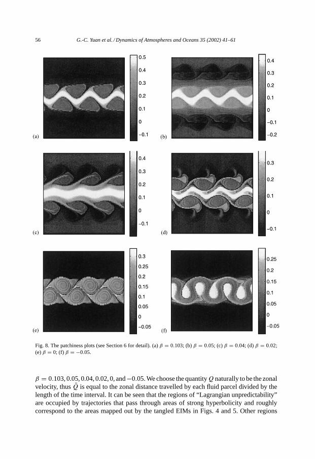
An efficient technique for quantifying initial condition sensitivity is thepatchiness plotfirst introduced by Malhotra et al. (1998) then developed by Poje et al. (1999). In essence,one computes the average of certain physical quantityQ along the parcel trajectory start-ing from an initial condition(x, y). Denote this average byQ(x, y). This computation isdone for every point (xi , yj ) from a rectangular grid. If two trajectories remain close formost of the time, then the averages corresponding to these trajectories are almost iden-tical. On the other hand, if for two nearby initial conditions (xi , yj ) and (xi′ , yj ′ ), thedifference|Q(xi , yj ) − Q(xi′ , yj ′)| is large, then the two trajectories must diverge fromeach other. The patchiness plot is the plot of the fieldQ versus the initial conditions(xi ,yj ), and it serves as an aid for identifying regions with initial condition sensitivity, char-acterized by large magnitude of|∇Q|. In Fig. 8(a)–(f ), we show the patchiness plots for


Fig. 8. The patchiness plots (see Section 6 for detail). (a)β = 0.103; (b)β = 0.05; (c)β = 0.04; (d)β = 0.02;(e)β = 0; (f) β = −0.05.

β = 0.103, 0.05, 0.04, 0.02, 0, and−0.05. We choose the quantityQnaturally to be the zonalvelocity, thusQ is equal to the zonal distance travelled by each fluid parcel divided by thelength of the time interval. It can be seen that the regions of “Lagrangian unpredictability”are occupied by trajectories that pass through areas of strong hyperbolicity and roughlycorrespond to the areas mapped out by the tangled EIMs in Figs. 4 and 5. Other regions


such as the jet core, the interiors of the vortex street eddies, and the Rossby wave dominatedfar fields show up with relative initial condition insensitivity.2

Advanced knowledge of the geometry and distribution of both regular and irregularregions is helpful in formulating strategies for launching Lagrangian instruments. If theintension is that the instrument remains in a certain feature, such as the jet core or an eddy,then the launch site should lie well in the interior of such features and away from the tangledmanifolds. On the other hand, studies of mixing may benefit from launch sites located inthe irregular regions.

Our study suggests that significant changes in the distribution and geometry of irregularregions may occur with depth. Near the surface of our model flow, irregular regions occuraround the edges of the cat’s eyes associated with the eastward-propagating meanders, asshown in part (a) of Figs. 4 and 8. Asβ is reduced (depth increases) secondary regions ofirregularity may emerge, one example being the “surf zone” (β = 0.05) shown in Figs. 5(a)and (d), and 8(b). For this flow, an observer moving northward or southward from the jetcore will encounter a regular region (the core), an irregular region in which regular poolsare embedded (the cat’s eyes), the regular band lying between the surf zone and the cat’seyes, the irregular surf zone itself, and finally the regular Rossby wave far field. Furtherreductions inβ lead to mergers of the cat’s eyes and surf zones (β = 0.04, Figs. 5(b) and(e), and 8(c)) resulting in the formation of a new set of cat’s eyes (β = 0.02, Figs. 5(c) and(f), and 8(d)). To this point, the irregular Lagrangian motion has been confined to the edgesof the jet and has not penetrated the central core itself. However, reduction toβ ≈ 0.01leads to destruction of the central barrier and formation of a vortex street across which theirregular motion can occur. The irregular region now has a braided geometry while regularregions consist of the vortices within the braids and the far field Figs. 4(b) and 8(e). Afurther slight reduction inβ leads to reformation of the central barrier and confinement ofthe irregular motion to homoclinic loops on either side of this barrier (Figs. 4(c) and 8(f )).

Characteristic regular and irregular motion in some of the regions just mentioned is shownin Fig. 9, which contains examples of parcel trajectories for flows withβ = 0.103, 0,−0.05.The initial positions of trajectories in irregular regions are marked ‘+’, while those in regularregions are marked ‘�’. The initial positions are also marked in the corresponding Fig. 2stream function maps. Trajectories originating at a ‘+’ do indeed appear more irregular thatthose originating at a ‘�’, the latter being nearly periodic. In some cases, pairs of trajectorieshave been initialized close together in order to observe initial condition sensitivity. The pairbeginning near the ‘+’ in Fig. 9(b), stays together for a brief period but rapidly divergethereafter. Note that the northern member of the pair crosses the vortex street and remainson the north side of the street, a good example of cross-street transport. The two ‘�’ pairsoriginating in the same figure remain together.

Ocean floats and drifters are not ordinarily launched in pairs, making it difficult to evaluateseparation rates. However, promising directions have recently been suggested in Lacasce

2 The spirals inside the eddies are rather curious. Similar patterns also appear in Poje et al. (1999) for barotropicturbulence, but the authors did not discuss the origin of this pattern. We find the underlying mechanism accountingfor the robustness of this spiral pattern is the combination of two factors. First, parcels inside the eddies rotatearound the eddy centers. Secondly, the locations of the eddies are not fixed but translated in time (in our case, wemean in the co-moving reference frame).


Fig. 9. Sample Lagrangian trajectories (in the stationary frame) for (a)β = 0.103; (b)β = 0; (c) β = −0.05.The initial positions are marked with ‘+’ or ‘ �’.

et al. (2000). In particular, they have calculated the separation rates for a collection ofinstruments that have been launched in pairs or have passed close to one another, in severalsections of the North Atlantic. They find that the mean square separations of most pairsinitially grows non-linearly. This may be explained by the initial velocities of the instrumentsdiffering by a small constant, but an alternative explanation is that different pairs havedifferent separation rates, and that certain pairs separate exponentially, as discussed in theabove. In fact, Lacasce et al. (2000) do find that certain pairs separate much faster thanothers. Unfortunately, their analysis is limited by the facts that the time series are very shortand that the data are contaminated by large noise. Therefore, they are not able to concludewhether there are pairs having exponential separation rates. They are currently working ondata collected from the Gulf of Mexico, which have better quality. It is expected that moreconclusive results will be obtained.


7. Conclusions and discussions

By decreasing the value ofβ in a model of a barotropic jet we have simulated the qua-litative changes expected to occur with increasing depth (or density) in certain surface-intensified, ocean jets. These changes include increased eastward meander propagationspeed relative to the background eastward fluid velocity, decreased potential vorticity dif-ference across the jet, and emergence of a flow with strong eddy motions and a weaker jetcharacter. We decreaseβ down to slightly negative values, deeming the latter consistentwith observed values near zero in the Gulf Stream. Within this range, destruction of thecentral potential vorticity barrier and consequent cross-flow transport is observed only inthe narrow windowW corresponding approximately to−0.01< β < 0.01. Similar win-dows are found for jets of different shapes. WithinW , the stream function contours in theco-moving reference frame take on a braided pattern that suggests separatrix reconnection.The corresponding flow has the character of a vortex street and transport across the street isdemonstrated by the intersecting unstable and stable EIMs associated with the hyperbolicregions lying to the north and south of the street.

Motivated by the fact that an oceanic flow is disturbed by many external forcings, wetest the strength of a transport barrier by introducing disturbances in our model. Althoughtransport is not observed for the casesβ > 0.01 (a meandering jet with a high potentialvorticity gradient core) andβ < −0.01 (a vortex street with a continuous band of highpotential vorticity gradient meandering between the vortices), transport can be forced inthese cases by varying the value ofβ. However, the effect of this forcing is asymmetric withrespect toβ. Forβ-values of equal magnitude but opposite sign, the fluctuation required todestroy the transport barrier is larger for the positiveβ than for the negative one. Withinthe fluctuation frequencies tested, the lowest of which permits four cycles over the finiteduration of the solution, the barrier is most easily penetrated at low frequency. It is strikingthat, forβ < 0, some disturbances may destroy the barrier without oscillating acrossW ;whereas forβ > 0, destruction of the barrier may only occur whenβ passes throughW .We also test the forcing due to a white noise disturbance ofβ. Again it is easier to destroythe transport barrier for negativeβ than for positiveβ.

The central question to be addressed next concerns the depth (or density) range that thewindowW corresponds to. Bower and Lozier (1994) estimations of monthly mean GulfStream potential vorticity gradient exhibit a good deal of temporal variability. For example,the potential vorticity gradient in a layer lying between 14.5 and 17.0 ◦C is significantlydifferent from zero for all but several months of the 20 month period of observations.Note that this layer lies between 500± 100 m depth at the south edge of the Gulf Streamand between 100± 30 m at the north edge. For the 7.0–9.5◦C layer, which extends from800 ± 50 m on the south side to 350± 50 m on the north side, the potential vorticitygradient is significantly different from zero for only a few of the 20 months. One mightchoose this and lower layers as candidates for separatrix reconnection and barrier destruc-tion. However the full baroclinic model is clearly required to explore this issue in moredepth.

It is not known whether the “homoclinic” vortex street found forβ < 0.01 is relevant tothe deep Gulf Stream. It is certainly possible to find potential vorticity profiles that exhibitnegative gradient across in the whole flow in the measurements of Bower and Lozier (1994).


Quoted error bars for these cases indicate that the apparently negative gradients are notsignificantly different from zero.

Although our model suggests a mechanism for fluid exchange across a jet, it does notexplain how fluid from afar can participate in this exchange. One must appeal to some largescale process such as the “cooling spiral” (Spall, 1992) to bring fluid into contact with theregion of chaotic advection. In Spall’s model, surface fluid in the North Atlantic subtropicalgyre circulates anticyclonically in a downwards spiral. The sinking is caused by cooling inthe western boundary layer and its extension. Due to dynamics analogous to theβ spiral,trajectories in the sinking region are forced to cross shallower trajectories from south tonorth. The net effect is that deep fluid is increasingly directed northwards, towards the axisof the jet separating the subtropical and subpolar gyres.

An incidental result of this investigation has been the observation of transitions in theflange region of the jet asβ approachesW from above. Just beforeW is reached, the(prograde) cat’s eyes associated with primary meander at highβ combine with a (retrograde)“surf zone” to form a new set of cat’s eyes. This merger creates relatively wide bands ofchaotic stirring in the flanges. Asβ entersW the new cat’s eyes merge and the centralbarrier is broken in what we call separatrix reconnection. Although the particulars of theflange transitions are likely model dependent, the existence and importance of secondarymodes (here the retrograde of Rossby waves) implies that the process leading to barrierdestruction at depth may not be as simple as previously thought. For example, Pratt et al.(1995) suggested a picture in which the jet is dominated in all depths by a normal modemeander. At the surface, a central barrier exists and chaotic stirring is confined to cat’s eyescentered around the critical latitudes of the meander, much as in part (a) of Figs. 2–4. Asone descends to deeper levels (or denser isopycnals) the critical latitudes move inwards andeventually merge, causing the central barrier to be broached. Our findings should serve as areminder that other disturbances, for example those associated with Rossby wave radiation,may emerge at deeper levels and may alter the chain of events.

Hyperbolic regions and their EIMs give an underlying geometry that provides tem-plates for chaotic stirring and transport of fluid in the jet. This study has identified arange of underlying geometries that could arise as depth is varied. Such changes wouldbe important in the design of float and drifter experiments. If the intent is for the in-strument to remain in certain regions, such as the jet core or a vortex structure, thenadvance knowledge of the locations of barriers and regions of enhanced stirring would bevaluable.

Acknowledgements

We thank Audrey Rogerson for providing her original numerical code. Chi-Wang Shuhelped us improve our numerical methods. The Lagrangian analysis is conducted usingPatrick Miller’s software:VFTOOL. We also thank Steve Meacham, Sanjeeva Balasuriyaand Susan Lozier for helpful discussions. Finally, the use of the patchiness plot techniquewas suggested to us by an anonymous reviewer, to whom we express our sincere gratitude.This research was funded by the Office of Naval Research Grant N00014-92-J-1481 andN10014-99-1-0258.


References

Behringer, R.P., Meyers, S.D., Swinney, H.L., 1991. Chaos and mixing in a geostrophic flow. Phys. Fluids A 3,1243–1249.

Bower, A.S., 1991. A simple kinematic mechanism for mixing fluid parcels across a meandering jet. J. Phys.Oceanogr. 21, 173–180.

Bower, A.S., Rossby, H.T., 1989. Evidence of cross-frontal exchange processes in the Gulf Stream based onisopycnal RAFOS float data. J. Phys. Oceanogr. 19, 1177–1190.

Bower, A.S., Lozier, M.S., 1994. A closer look at particle exchange in the Gulf Stream. J. Phys. Oceanogr. 24,1399–1418.

Bower, A.S., Rossby, H.T., Lillibridge, J.L., 1985. The Gulf Stream: barrier or blender? J. Phys. Oceanogr. 15,24–32.

Cronin, M., Watts, D.R., 1996. Eddy mean flow interaction in the Gulf Stream at 68◦W. J. Phys. Oceanogr. 26,2107–2131.

del-Castillo-Negrete, D., Morrison, P.J., 1993. Chaotic transport by Rossby waves in shear flow. Phys. Fluids A5 (4), 948–965.

Duan, J.Q., Wiggins, S., 1996. Fluid exchange across a meandering jet with quasi-periodic time variability. J. Phys.Oceanogr. 26, 1176–1188.

Dutkiewicz, S., Griffa, A., Olson, D.B., 1993. Particle diffusion in a meandering jet. J. Geophys. Res. 98 (C9),16487–16500.

Flierl, G.R., Malanotte-Rizzoli, P., Zabusky, N.J., 1987. Non-linear waves and coherent vortex structures inbarotropicβ-plane jet. J. Phys. Oceanogr. 17, 1408–1438.

Haller, G., Poje, A.C., 1998. Finite time transport in aperiodic flows. Physica D 119, 352–380.Hogg, N.G., 1988. Stochastic wave radiation by the Gulf Stream. J. Phys. Oceanogr. 18, 1687–1701.Lacasce, J.H., Bower, A.S., Zhang, H, 2000. Relative dispersion in the subsurface North Atlantic. J. Mar. Res.,

submitted for publication.Lozier, M.S., Bercovici, D., 1992. Particle exchange in an unstable jet. J. Phys. Oceanogr. 22, 1506–1516.Malhotra, N., Mezic, I., Wiggins, S., 1998. Patchiness: a new diagnostic for Lagrangian trajectory analysis in

time-dependent fluid flows. Int. J. Bifurcation Chaos Appl. Sci. Eng. 8, 1053–1093.Malhotra, N., Wiggins, S., 1998. Geometric structures, lobe dynamics, and Lagrangian transport in flows with

aperiodic time-dependence, with applications to Rossby wave flow. J. Non-linear Sci. 8, 401–456.Meyers, S.D., 1994. Cross-frontal mixing in a meandering jet. J. Phys. Oceanogr. 24, 1641–1646.Miller, P.D., Jones, C.K.R.T., Rogerson, A.M., Pratt, L.J., 1997. Quantifying transport in numerically generated

vector fields. Physica D 110, 105–122.Ngan, K., Shepherd, T.G., 1997. Chaotic mixing and transport in Rossby wave critical layers. J. Fluid Mech. 334,

315–351.Pedlosky, J., 1987. Geophysical Fluid Dynamics, (2nd edition). Springer. 710 pp.Poje, A.C., Haller, G., Mezic, I., 1999. The geometry and statistics of mixing in aperiodic flows. Phys. Fluids 11,

2963–2968.Pratt, L.J., Lozier, M.S., Beliakova, N., 1995. Parcel trajectories in quasi-geostrophic jets: neutral nodes. J. Phys.

Oceanogr. 25, 1451–1466.Rogerson, A.M., Miller, P.D., Pratt, L.J., Jones, C.K.R.T., 1999. Lagrangian motion and fluid exchange in a

barotropic meandering jet. J. Phys. Oceanogr. 29, 2635–2655.Samelson, R.M., 1992. Fluid exchange across a meandering jet. J. Phys. Oceanogr. 22, 431–440.Savidge, D.K., Bane, J.M., 1999a. Cyclogenesis in the deep ocean beneath the Gulf Stream. 1. Description.

J. Geophys. Res. 104 (C8), 18111–18126.Savidge, D.K., Bane, J.M., 1999b. Cyclogenesis in the deep ocean beneath the Gulf Stream. 2. Dynamics.

J. Geophys. Res. 104 (C8), 18127–18140.Spall, M., 1992. Cooling spirals and recirculation in the subtropical gyre. J. Phys. Oceanogr. 22, 564–571.Wiggins, S., 1992. Chaotic Transport in Dynamical Systems. Interdisciplinary Applied Mathematics, Vol. 2.

Springer, Berlin, 301 pp.

barrier destruction and lagrangian predictability at depth in a

Documents