Geometric Concepts in PhysicsPaul Duffell

Based on lectures by Brian Greene

Illustrations by Andrew Macfarlane

Table of Contents

Introduction 31. Review of Manifold Concepts 6

1.1 The Exponential Map 61.2 Pushforward and Pullback 101.3 The Lie Derivative 16

2. Group Theory 222.1 Groups 222.2 Extracting Groups out of Groups 272.3 Morphisms 282.4 Quotient Groups 322.5 Group Action on a Set 332.6 Fields and Algebras 34

3. Lie Groups 363.1 Matrix Groups 373.2 The Tangent Space of a Lie Group 383.3 From the Group to the Algebra and Back Again 413.4 The Rest of the Lie Algebra Story 473.5 Realizations and Representations 493.6 Summary and Application 53

4. Fiber Bundles 554.1 Product Manifolds: A Visual Picture 554.2 Fiber Bundles: The Informal Description 564.3 Fiber Bundles: The Bloated Description 594.4 Special Types of Fiber Bundles 60

4.5 Fiber Bundles: The More Elegant Description 644.6 Curvature: Generalizing Past the Tangent Bundle 654.7 Parallel Transport on General Fiber Bundles 694.8 Connections on Associated Vector Bundles 73

Introduction

This text is intended for a student who has already studied some geometry. It will beassumed that the reader is familiar with topology, manifolds, tangent spaces, tensors,differential forms, metrics, connections, and curvature. If it is useful to the interestedreader, I may eventually supplement this work with background material, but this will mostlikely be unnecessary, as there are a great many sources which treat these basic foundationalconcepts.

Einstein's general theory of relativity was an incredibly beautiful discovery. Thenotion that gravity can be described without forces, purely geometrically, is as compelling aconcept today as it was in the 1920's. Even more impressive is the fact that this simpleobservation of a beautiful mathematical description of a physical phenomenon lead to atheory of gravity which was more precise and accurate than any theory ever considered, andremains so to this day. The construction of this theory didn't require any physicalobservation; Einstein was just trying to look at gravity in a more mathematically appealingway. In doing so, he improved the theory in ways that went far beyond this elegant aesthetic.

It is in this spirit that we seek to study Einstein's final accomplishment: a classicalunified theory. We shall see how it is possible to characterize every force (not just gravity) inan entirely geometric language. The mathematical machinery we'll need will not be trivial,but the payoff is certainly worth the effort. We'll begin by reviewing a few useful conceptswhich may or may not be second-nature to you already. As stated before, you should alreadyknow all about manifolds, but you may not have a very strong background in the theory of

groups, so I also include a decent introduction to this subject (or perhaps just a refresher).We will then plunge deep into the subject of lie groups, followed by fiber bundles, andfinally reviewing the ideas of connections and curvature (in which you should be fluent),generalizing these concepts as far as they will go. When we are done, it will be possible towrite down a geometric physical theory which describes all of the forces of the universe. Atsome point, a section will be included which gives some treatment of the physicalapplications, but currently this part will have to be found in supplementary material. Thisphysical theory is the big payoff, and I don't wish to rob you of it, so I tentatively label thiswork a “first edition”, with improvements to come.

The problems provided are generally not very challenging, but are meant to keep thereader involved in the material. I personally find that a page full of equations is asaesthetically displeasing as it is unenlightening, and whenever the opportunity arises totrade a block of equations in exchange for a guided exercise for the reader, I feel it's a tradeworth making. In later editions, I may add more challenging exercises to the end of eachsection, but as of now I don't feel the necessity.

As stated before, this is a work in progress. I take pride in my attention to detail, butthis does not mean I'm always right. Contact me, if you find any problem with my clarity,consistency of notation, or even grammar. Good writing requires good feedback, especiallyin the case of technical writing. In any case, I'd like to avoid too long an introduction, so letus get right to the mathematics; I hope your experience with these concepts is as enjoyableas mine has been.

1

Review of Manifold Concepts

There are some preliminary odds and ends that we need to cover before leaping intolie groups. Specifically, we'll need to clearly understand the exponential map, thepushforward and pullback maps, and finally the lie derivative. These concepts will be usedagain and again, and so a fairly thorough treatment is given, in the hopes that yourunderstanding becomes as complete as possible.

1.1 The Exponential Map

This is a map which provides a concrete relationship between the tangent space of amanifold, and the manifold itself. There are many ways to conceptually approach theexponential map, so a couple of different approaches are given.

From the Infinitesimal to the Macroscopic

Often in mathematics (and very often in physics), one deals with the effect on aλ λ ε λ εfunction f( ) when we change by a small parameter, . Formally, we can expand f( + ) in

λa taylor series about :

f = f dfd

½2 d2 fd 2

... (1.1)

ε εIf is infinitesimally small, we can ignore terms of order greater than ² and the result issimply:

f =1 dd

f (1.2)

ε λIt is possible to regard this as an operator, T( ), acting on f( ), whose operation is to translate

λ ε by an infinitesimal amount, .f =T f

Δλ λWhat if we want a more general operator, T( ), whose operation translates by aΔλfinite amount, ? We could easily read off this operator from the fully-expanded power

series above, but it is more instructive to think of this finite-translation operator as aproduct of a large amount of successive infinitesimal-translation operators:T =[T ]N ,where=N⋅ (1.3)

We then take the limit as N → ∞. In other words,

T = limN ∞

[1N

dd

]N

(1.4)

Does this formula look familiar yet? Let us pretend for the time being that theΔλ λoperator ( d/d ) is just a number, k. Then the formula looks like:

T = limN ∞

[1 kN]N

(1.5)

This you should recognize as a definition of the exponential function, ek. We carry thenotation over to describe the translation operator:

T =e d

d (1.6)

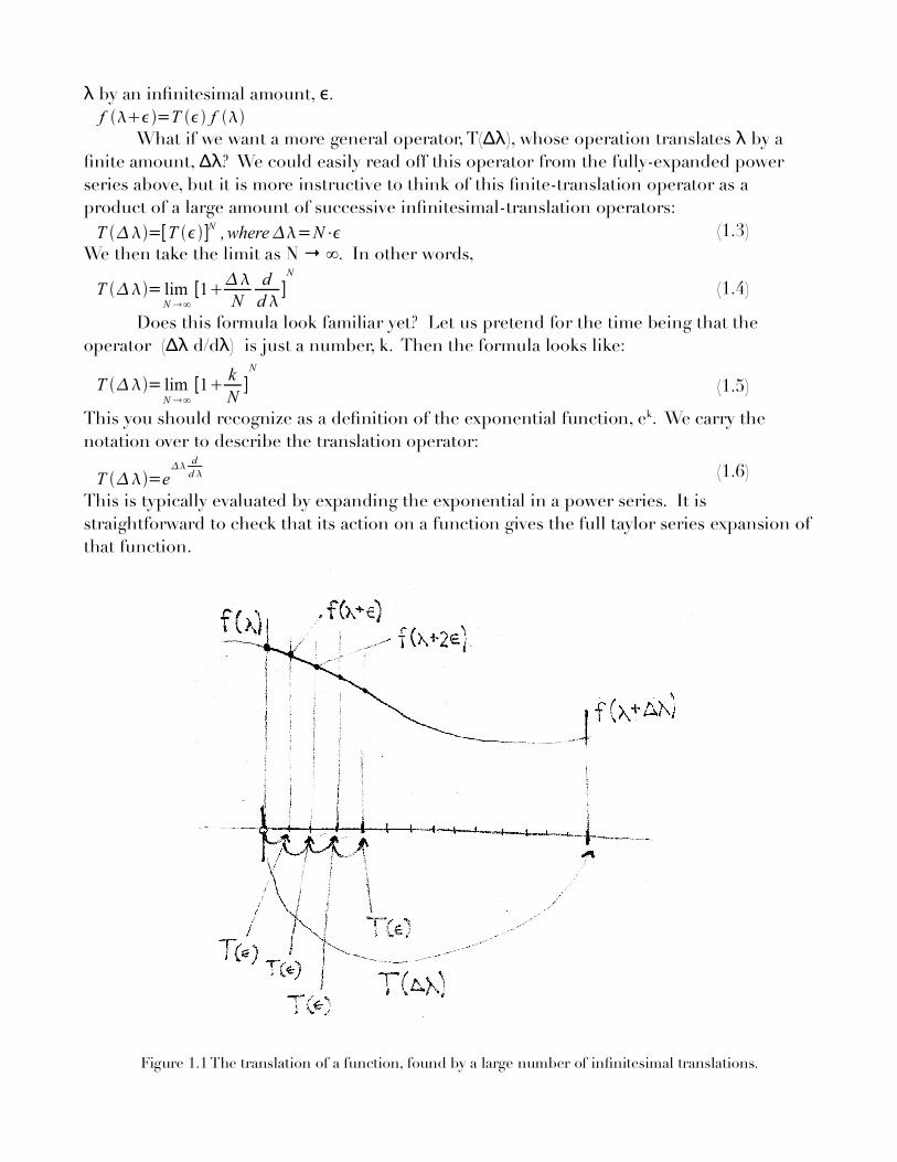
This is typically evaluated by expanding the exponential in a power series. It isstraightforward to check that its action on a function gives the full taylor series expansion ofthat function.

Figure 1.1 The translation of a function, found by a large number of infinitesimal translations.

Problem 1.1 Check that the exponential map's action on a function gives the taylor seriesλ λexpansion of the function; that is, check that it appropriately translates f( ) by a distance Δ .

Now, we make a small conceptual transition. Instead of thinking of this as anΔλoperator-valued function with respect to the inverval, , it is more natural to think of it as

Δλ λan operator-valued function on derivatives, d/dt = d/d . In other words, we can vary theλtranslation distance by varying our reparameterization, t = t( ). So, we symbolically write

this as

T ddt=ed /dt (1.7)

This is a more natural form of our translation operator, the exponential map. You can thinkof this as generating a translation, T, given a derivative, d/dt.

From Vector Fields to Integral Curves

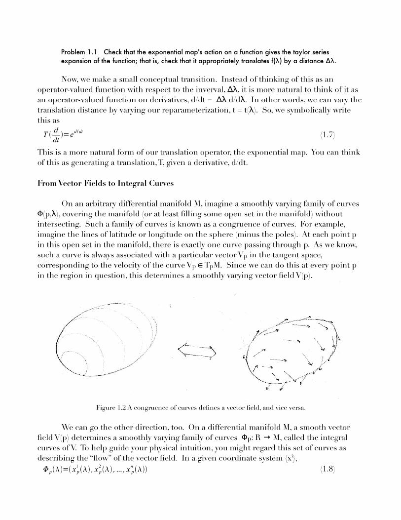
On an arbitrary differential manifold M, imagine a smoothly varying family of curvesΦ λ(p, ), covering the manifold (or at least filling some open set in the manifold) withoutintersecting. Such a family of curves is known as a congruence of curves. For example,imagine the lines of latitude or longitude on the sphere (minus the poles). At each point pin this open set in the manifold, there is exactly one curve passing through p. As we know,such a curve is always associated with a particular vector Vp in the tangent space,corresponding to the velocity of the curve Vp ∈ TpM. Since we can do this at every point pin the region in question, this determines a smoothly varying vector field V(p).

Figure 1.2 A congruence of curves defines a vector field, and vice versa.

We can go the other direction, too. On a differential manifold M, a smooth vectorΦfield V(p) determines a smoothly varying family of curves p →: R M, called the integral

curves of V. To help guide your physical intuition, you might regard this set of curves asdescribing the “flow” of the vector field. In a given coordinate system {xi}, p= x p

1 , x p2 , ... , x p

n (1.8)

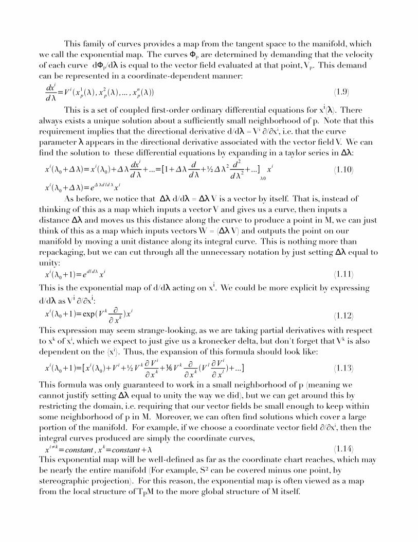
This family of curves provides a map from the tangent space to the manifold, whichΦwe call the exponential map. The curves p are determined by demanding that the velocity

Φof each curve d p λ/d is equal to the vector field evaluated at that point, Vp. This demandcan be represented in a coordinate-dependent manner:dxi

d =V i x p

1 , x p2 ,... , x p

n (1.9)

This is a set of coupled first-order ordinary differential equations for xi λ( ). Therealways exists a unique solution about a sufficiently small neighborhood of p. Note that this

λrequirement implies that the directional derivative d/d = Vi ∂/∂xi, i.e. that the curveλparameter appears in the directional derivative associated with the vector field V. We can

Δλfind the solution to these differential equations by expanding in a taylor series in :

xi0= xi0 dxi

d ...=[1 d

d ½2 d

2

d 2...]

0

xi (1.10)

xi0=ed /d xi

Δλ λ ΔλAs before, we notice that d/d = V is a vector by itself. That is, instead ofthinking of this as a map which inputs a vector V and gives us a curve, then inputs a

Δλdistance and moves us this distance along the curve to produce a point in M, we can justΔλthink of this as a map which inputs vectors W = ( V) and outputs the point on our

manifold by moving a unit distance along its integral curve. This is nothing more thanΔλrepackaging, but we can cut through all the unnecessary notation by just setting equal to

unity:xi01=e

d / d xi (1.11)

λThis is the exponential map of d/d acting on xi. We could be more explicit by expressing

λd/d as Vi ∂/∂xi:

xi01=expVk ∂∂ xk

xi (1.12)

This expression may seem strange-looking, as we are taking partial derivatives with respectto xk of xi, which we expect to just give us a kronecker delta, but don't forget that Vk is alsodependent on the {xi}. Thus, the expansion of this formula should look like:

xi01=[ xi0Vi½V k ∂V i

∂ x k⅙V k ∂

∂ x kV l ∂V i

∂ xl...] (1.13)

This formula was only guaranteed to work in a small neighborhood of p (meaning weΔλcannot justify setting equal to unity the way we did), but we can get around this by

restricting the domain, i.e. requiring that our vector fields be small enough to keep withinsome neighborhood of p in M. Moreover, we can often find solutions which cover a largeportion of the manifold. For example, if we choose a coordinate vector field ∂/∂xi, then theintegral curves produced are simply the coordinate curves,xi≠k=constant , x k=constant (1.14)

This exponential map will be well-defined as far as the coordinate chart reaches, which maybe nearly the entire manifold (For example, S² can be covered minus one point, bystereographic projection). For this reason, the exponential map is often viewed as a mapfrom the local structure of TpM to the more global structure of M itself.

1.2 Pushforward and Pullback

The pushforward and pullback maps are natural ways of mapping objects like vectorsΦand forms from one differential manifold to another, given a map : M₁ → M₂ between

points on the manifolds. The concepts here are somewhat abstract, but they can beconcretely represented in computational form when we look at specific coordinate systemson the manifolds.

The Pullback of a Function

We start with two manifolds, M₁ and M₂, of dimension n₁ and n₂, respectively.ΦAdditionally, we have a smooth map : M₁ → M₂. This map need only be well-defined and

smooth; it does not have to be a one-to-one map, nor does it have to map onto the entiremanifold M₂. Now, let's look at the space of smooth functions f(q) on points {q} in M₂. Isthere a natural way to map these to the set of functions g(p) on points {p} in M₁? That is,

Φgiven a function f(q), can we use the map to naturally produce a function g(p) defined onM₁?

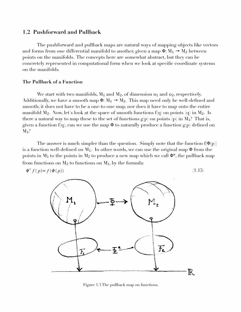
ΦThe answer is much simpler than the question. Simply note that the function f( (p))is a function well-defined on M₁ Φ. In other words, we can use the original map from thepoints in M₁ to the points in M₂ Φ to produce a new map which we call *, the pullback mapfrom functions on M₂ to functions on M₁, by the formula:

∗ f p= f p (1.15)

Figure 1.3 The pullback map on functions.

This is clearly well-defined; given any smooth function f(q) on M₂, we can always use thisΦformula to produce a function g(p) = f( (p)) on M₁. The pullback map is not generally one-

to-one, nor does it always map onto the entire space of smooth functions on M₁. In otherΦwords, we cannot generally “push foward” functions. In the special case that is invertible,

Φso is *; we can push functions forward simply by using the pullback of the inverse map.

Problem 1.2 Φ Φ Φ Φ Show that when is injective, * is surjective, and when is surjective, * isΦ Φinjective. Thus, when is bijective, so is *.

To summarize, the pullback of a function defined on M₂ is simply the function'srepresentation on points in M₁ which get mapped to points in M₂ Φ by the map .

The Pushforward of a Vector

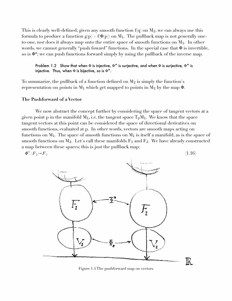
We now abstract the concept further by considering the space of tangent vectors at agiven point p in the manifold M₁, i.e. the tangent space TpM₁. We know that the spacetangent vectors at this point can be considered the space of directional derivatives onsmooth functions, evaluated at p. In other words, vectors are smooth maps acting onfunctions on M₁. The space of smooth functions on M₁ is itself a manifold, as is the space ofsmooth functions on M₂. Let's call these manifolds F₁ and F₂. We have already constructeda map between these spaces; this is just the pullback map:∗: F 2F 1 (1.16)

Figure 1.4 The pushforward map on vectors.

Since vectors in TpM₁ are themselves linear maps on F₁, we should be able to find anatural map to vectors on F₂, by pulling back again. We have to check that this map indeedproduces a directional derivative, and not just some general map, but for now accept that itwill.

What does this map look like? Given a vector V in TpM₁, this is a directionalderivative map on functions on M₁, given by the formula:

V [ g p]=V i ∂ g∂ xi

∣p (1.17)

where {xi} is a local coordinate system in the vicinity of p on M₁. Now use the pullback mapon functions to get a vector acting on functions in M₂. This is what we will call the

Φ⁎pushforward map, :∗V [ f q]=V [∗ f p ]=V [ f p] (1.18)

Let's get our head straight about things. V is a map on functions on M₁. f(q) is a functionon M₂ Φ⁎. Thus, V can't act directly on f. V is a vector field defined on M₂, which can act on

Φfunctions f(q). *f is a function on M₁, which can be acted on by V.

Computation

We can just use the chain rule to evaluate this:

∗V [ f q]=V [ f p]=V i ∂ f∂ xi

=V i ∂k

∂ xi ∂ f∂k (1.19)

=V i ∂ yk

∂ xi ∂ f∂ yk

(1.20)

Here, we are also using a local coordinate chart on M₂, {yk}. We have simplified the notationΦby expressing (p) in both of the coordinate representations as yk(xi). The last expression is

clearly a directional derivative, thus this genuinely pushes vectors from TpM₁ to TΦ(p)M₂ (notjust to the space of general maps acting on functions in M₂).

We now have a natural map from TpM₁ to TΦ(p)M₂. We can realize this map as amatrix Aik = ∂yk/∂xi acting on vectors in TpM₁. Aik is an n₂ × n₁ matrix, mapping the n₁components of V to the n₂ Φ⁎ components of V. Note that Aik is coordinate-dependent. Note

Φalso that we can push vectors forward, but we cannot pull them back, unless has aninverse. In other words, Aik is not generally an invertible matrix (it might not even have thesame number of rows as columns).

Another way to see how the pushforward map acts on vectors is to look at anothernatural manifestation of the tangent vector space TpM₁: velocities of curves passing through

Φp. Since maps points in M₁ to points in M₂, it naturally maps curves in M₁ to curves inM₂, hence it can map velocities from one manifold to the other. It is easy to show that thisleads to the same pushforward map that we defined on directional derivatives. The velocityof the mapped curve is given by the same chain rule as above. This is a nice way of picturing

the pushforward map on vectors, as it requires no computation to properly visualize.

Problem 1.3 Show that the pushforward map defined as the naturally induced map fromvelocities of curves in M1 to velocities of curves in M2 gives the same chain rule as above.

The Pullback of a One-Form

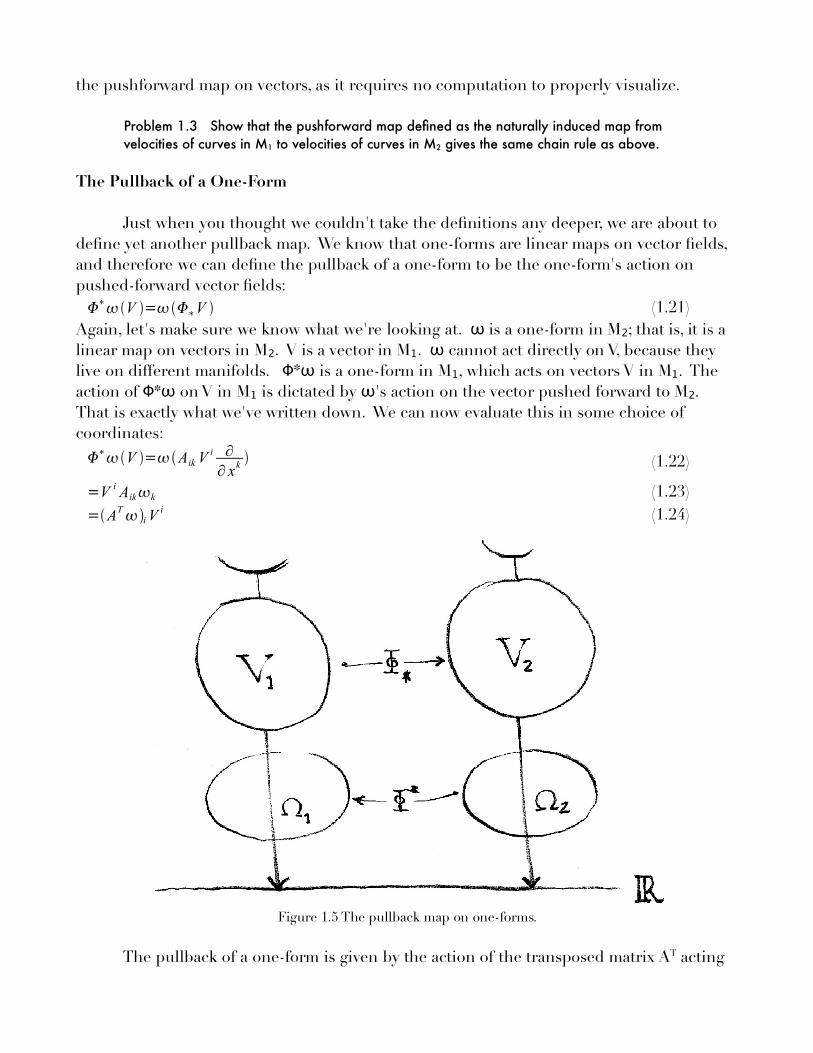
Just when you thought we couldn't take the definitions any deeper, we are about todefine yet another pullback map. We know that one-forms are linear maps on vector fields,and therefore we can define the pullback of a one-form to be the one-form's action onpushed-forward vector fields:∗V =∗V (1.21)

ωAgain, let's make sure we know what we're looking at. is a one-form in M₂; that is, it is alinear map on vectors in M₂. V is a vector in M₁ ω. cannot act directly on V, because they

Φ ωlive on different manifolds. * is a one-form in M₁, which acts on vectors V in M₁. TheΦ ωaction of * on V in M₁ ω is dictated by 's action on the vector pushed forward to M₂.

That is exactly what we've written down. We can now evaluate this in some choice ofcoordinates:∗V =Aik V

i ∂∂ xk

(1.22)

=V i Aikk (1.23)=ATi V

i (1.24)

Figure 1.5 The pullback map on one-forms.

The pullback of a one-form is given by the action of the transposed matrix AT acting

on its components. We might have expected this, especially if we note that A is an n₂ × n₁matrix, while AT is an n₁ × n₂ matrix, which is exactly what we'd need to send the n₂

ωcomponents of to an n₁-component one-form defined on M₁.

In general, we can pull back any (0,k) tensor, and push forward any (k,0) tensor, thegeneralization being to simply multiply by additional copies of the matrix A or AT.However, we cannot do the reverse, nor can we push or pull any (l,m) tensor, for nonzero l

Φ Φand m, unless is invertible. In the case where is invertible, it is possible to push or pulltensors of any rank, essentially by multiplying by inverse matrices, where applicable.Obviously there are some details to be filled in, but this is the basic idea.

Problem 1.4 Derive the pushforward and pullback formulas for tensors of arbitrary rank,Φgiven an invertible map between the manifolds, with a corresponding pushforward matrix

A.

A good example shows up in the coordinate charts on a differential manifold, M.ΦNotice that any coordinate chart (usually also labeled , which might normally confuse us,

but in this case they are referring to the same function) is an invertible map between an

open set in M and an open set in Rn. Therefore, we can pull functions on open sets in M

back to functions on open sets in Rn. This is how we define things like continuity,differentiability, and in the case of complex manifolds, analyticity. We pull functions back to

Rn, and evaluate these properties in a more concrete setting.

We can also push vectors forward from Rn to TpM, using a coordinate chart in aneighborhood of p. This is essentially what we are doing when we determine the

Φcomponents of a vector V in a given coordinate system, given by . Different coordinatecharts will generally give us different pushforward maps, which in turn give us differentcomponents for V.

The Special Case M₁ = M₂

Set M₁ = M₂ Φ → = M. In other words, look at bijective maps : M M from a manifoldΦonto itself. In particular, look at a smoothly varying family of such maps, { pq Φ}, where pq is

a smooth, bijective map from M onto itself, which maps p to q. An example of this is thefamily of rotations on the manifold of S¹, the circle. For any two points p and q on the

Φcircle, there is a unique rotation pq which sends p to q.

ΦWe can define -invariant vector fields on M to be vector fields which are invariantΦunder the pushforward map pq⁎: Tp →M Tq ΦM. Thus, V(q) = pq⁎ ΦV(p). The set of -

invariant vector fields forms a vector space, since any two invariant vector fields can beΦadded together to find another invariant vector field, due to 's linearity. It is easily seen

that this vector space is equivalent to TpM at any point p in the manifold, since we can push

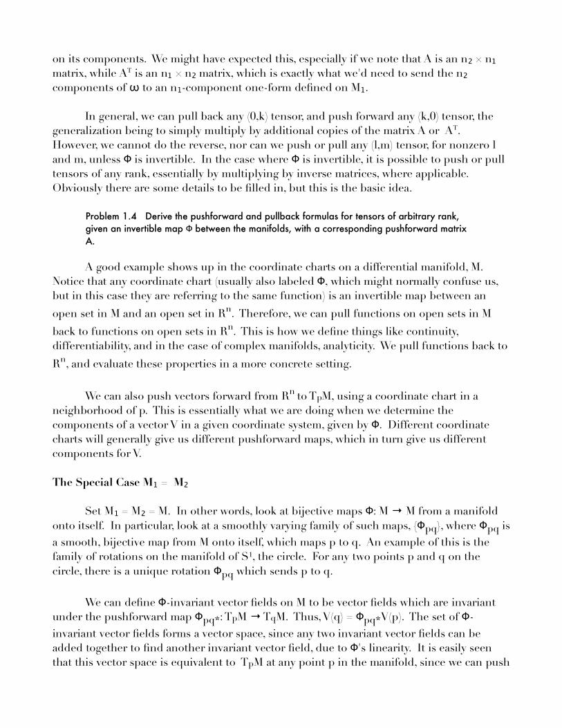
any tangent vector Vp Φ forward from p to every point q in the manifold, using pq⁎,Φproducing a manifestly invariant vector field: V(q) = pq⁎Vp. Since we can do this for any

Φvector V at p, and since pq is bijective (by assumption here), we can output a uniqueinvariant vector field V(q) given any vector Vp at p. Going back the other direction is eveneasier. Given an invariant vector field, we can get a unique vector Vp in TpM, simply byevaluating the vector field at p: Vp = V(p). Notice that both of these identifications are linear.

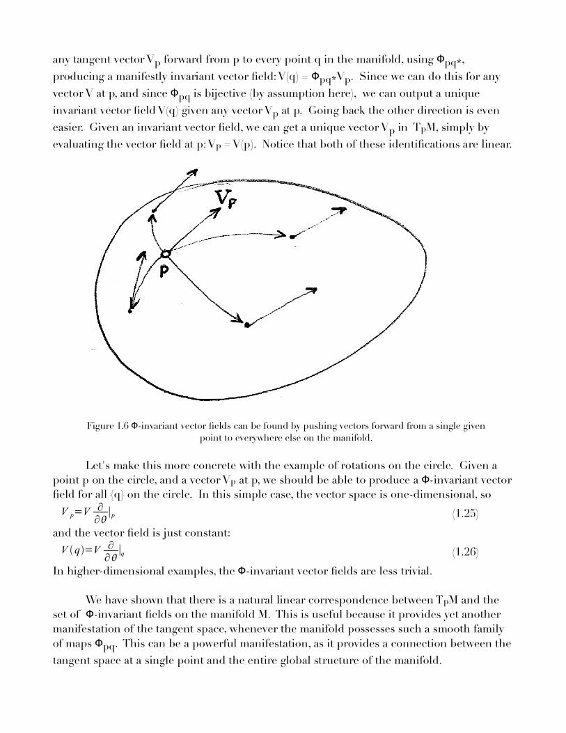
Figure 1.6 Φ -invariant vector fields can be found by pushing vectors forward from a single givenpoint to everywhere else on the manifold.

Let's make this more concrete with the example of rotations on the circle. Given apoint p on the circle, and a vector Vp Φ at p, we should be able to produce a -invariant vectorfield for all {q} on the circle. In this simple case, the vector space is one-dimensional, so

V p=V ∂∂

∣p (1.25)

and the vector field is just constant:V q=V ∂

∂∣q (1.26)

ΦIn higher-dimensional examples, the -invariant vector fields are less trivial.

We have shown that there is a natural linear correspondence between TpM and theΦset of -invariant fields on the manifold M. This is useful because it provides yet another

manifestation of the tangent space, whenever the manifold possesses such a smooth familyΦof maps pq. This can be a powerful manifestation, as it provides a connection between the

tangent space at a single point and the entire global structure of the manifold.

Problem 1.5 For the manifold Rn, the set of n-dimensional translations provides such a smoothΦfamily of maps. Show that -invariant vector fields in this case are given simply by constant

vector fields.

Problem 1.6 Consider the manifold given by R²\{0}, the plane minus the origin. Considermapping this space to itself, mapping a point p to another point q by the following algorithm:rotate the plane by the angle p and q make with the origin. Then scale the plane by the ratioof the distances from q and p (respectively) to the origin. First, show that this always gives asmooth map from the plane to itself which sends p to q. Then, pick two linearly independent

Φvectors at any point, and find their corresponding -invariant vector fields.

1.3 The Lie Derivative

A lie derivative provides a way of taking derivatives of vector fields on a manifold.Computationally, it can be quite simple, though conceptually it's actually very subtle. Ondifferential manifolds, it will be useful to be able to take derivatives of vector fields, but untilwe provide additional information, the concept of a “derivative” of a vector field is not well-defined.

Comparing Tangent Vectors

We want to think of the derivative as “the rate at which a vector field changes as wemove in some direction” in the manifold. This implies we are comparing tangent vectorsdefined at different points p and q in M. There is no canonical way to do this, since tangentvectors at p live in the tangent space TpM, and vectors at q live in a different space, TqM.There are many ways of defining maps between these two spaces, but there is no special ornatural map. Choosing a particular map between tangent spaces imposes additionalstructure, and this is usually fleshed out in the form of a connection, which gives us thecovariant derivative. The lie derivative provides an alternative method for differentiatingvector fields, which does not require a connection. Instead, the additional informationspecified to compare tangent vectors will be a congruence of curves.

Congruence of Curves

We mentioned this concept earlier, but it's worth restating. A congruence of curvesdefined on some neighborhood in a manifold M is a smoothly varying family of curveswhich fill this neighborhood, without intersecting. Each point in this neighborhood lies onexactly one such curve.

The key concept which allows the lie derivative to function conceptually is therelationship between vector fields and congruences of curves. Given a congruence ofcurves, we can find a vector field by taking at each point the velocity of the integral curvepassing through that point. We can also get a congruence of curves from a vector field,

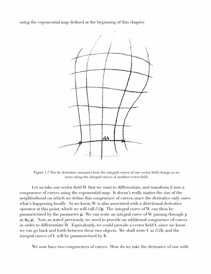
using the exponential map defined at the beginning of this chapter.

Figure 1.7 The lie derivative measures how the integral curves of one vector field change as wemove along the integral curves of another vector field.

Let us take our vector field W that we want to differentiate, and transform it into acongruence of curves using the exponential map. It doesn't really matter the size of theneighborhood on which we define this congruence of curves, since the derivative only careswhat's happening locally. As we know, W is also associated with a directional derivative

μoperator at this point, which we will call ∂/∂ . The integral curve of W can then beμparameterized by the parameter . We can write an integral curve of W passing through p

αas p μ( ). Now, as stated previously, we need to provide an additional congruence of curvesin order to differentiate W. Equivalently, we could provide a vector field V, since we know

λwe can go back and forth between these two objects. We shall write V as ∂/∂ , and theλintegral curves of V will be parameterized by .

We now have two congruences of curves. How do we take the derivative of one with

respect to the other? Conceptually, we want to look at how the curves of W change when weΔλmove a small distance along curves of V. We still have to deal with the issue of

comparing vectors at different points in the manifold; we've just transformed the probleminto comparing curves at different points in the manifold. Fortunately, the congruence ofcurves given by V gives us a natural way of transporting a curve of W to different points onthe manifold. We can define a new congruence of curves about the point p in the followingmanner:

Lie Dragging

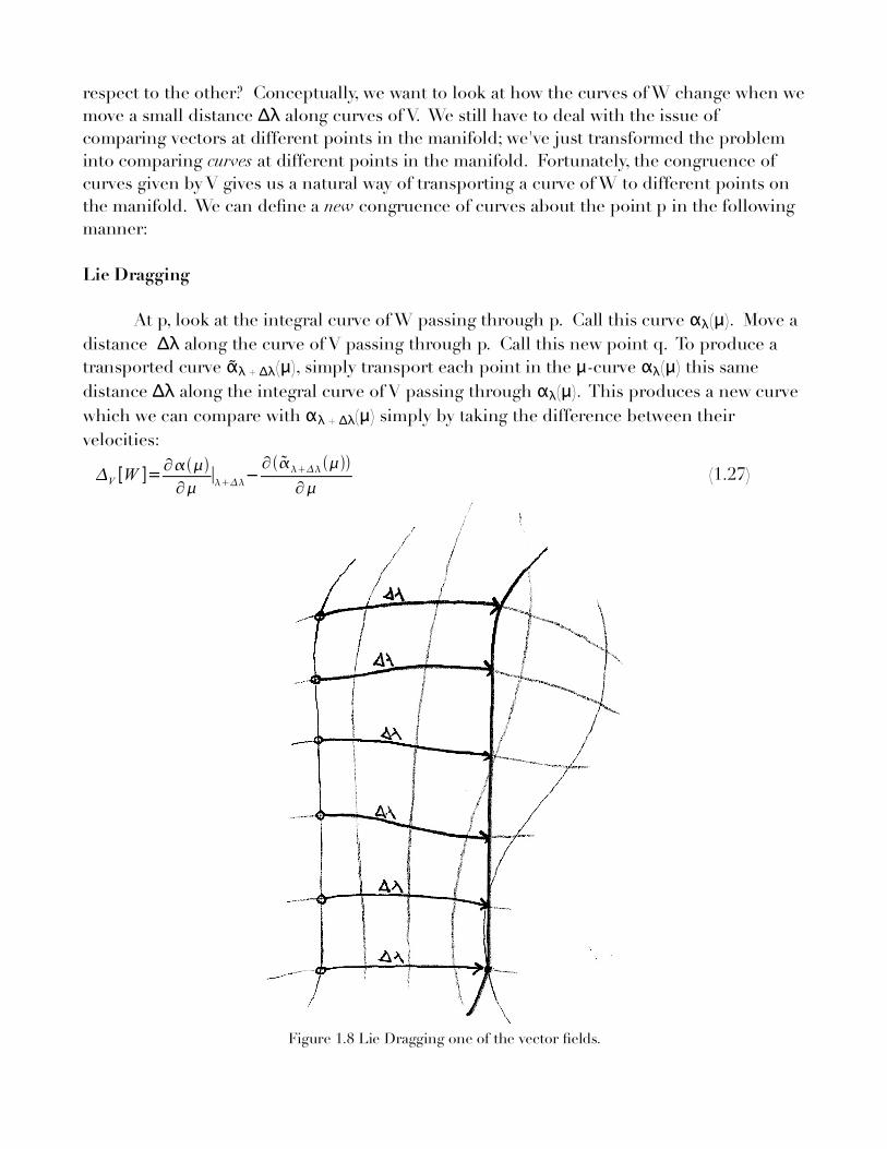
αAt p, look at the integral curve of W passing through p. Call this curve λ μ( ). Move aΔλdistance along the curve of V passing through p. Call this new point q. To produce a

ᾶtransported curve λ Δλ + μ μ α( ), simply transport each point in the -curve λ μ( ) this sameΔλ αdistance along the integral curve of V passing through λ μ( ). This produces a new curve

αwhich we can compare with λ Δλ + μ( ) simply by taking the difference between theirvelocities:

V [W ]=∂∂

∣−∂

∂(1.27)

Figure 1.8 Lie Dragging one of the vector fields.

A note about notation: we've introduced several concepts at once, and it's good toαkeep our head on straight about why things are written down the way they are. λ μ( ) is an

μ λintegral curve of W passing through p with parameter . We write the subscript “ ” insteadof “p” to accentuate the fact that p is given as a point on an integral curve of V,

λ αparameterized by . λ Δλ + μ( ) is simply another integral curve of W, this one instead passingΔλ ᾶthrough q, the point found by moving a distance along an integral curve of V. λ Δλ + μ( ) is

not α an integral curve. It is the curve found by transporting λ μ Δλ( ) a distance along integralμ αcurves of V passing through each of λ μ( ). The family of curves produced in this manner

αis said to be lie dragged. λ Δλ + μ ᾶ( ) and λ Δλ + μ( ) intersect each other at q, which is why wecan compare their velocities.

α ᾶIt is important to understand why the velocities of and are written the way theyαare. Since λ Δλ + μ( ) is an integral curve of W, the velocity of this curve is exactly what we

mean by Wq, the vector field evaluated at q. This is found by taking the derivative withμ λrespect to of integral curves at arbitrary , then evaluating it specifically at the point q,

λ Δλ ᾶwhich corresponds to + . For , we must first transport the curve before computing itsλ Δλvelocity. This is noted symbolically by putting the subscript + inside the parentheses.

This will become important shortly.

Computation of the Lie Derivative

Δλ ΔλWe can turn this difference into a derivative by dividing by and taking the limit as vanishes. This specifies the lie derivative:

ᏝV [W ]= lim∞

1

[∂∂

∣−∂

∂] (1.28)

The simplest way to compute this is to expand these terms to first order in a taylor series inΔλ Δλ →, since higher-order terms will vanish in the limit 0. This is an exercise left to thereader. Eventually, we arrive at the following:ᏝV [W ]= ∂

∂∂∂

− ∂∂

∂∂

(1.29)

Problem 1.7 Expand equation (1.28) in a first-order taylor series, deriving equation (1.29).

If we express this result in a particular coordinate system, we find that the secondderivatives cancel:

ᏝV [W ]i=[V j ∂W k

∂ x j−W j ∂V k

∂ x j]∂i ∂ xk

(1.30)

αWe've been interpreting this as the velocity of a curve, , but we can now think of this as a

αdirectional derivative operator acting on the coordinate function iλ μ( ) = xi

λ μ( ). Thederivative will just give us a kronecker delta, giving the following result:

ᏝV [W ]i=V j ∂W i

∂ x j−W j ∂V i

∂ x j(1.31)

We usually express this as the commutator [V,W], the result of commuting directionalderivative operators V and W. Written this way, it is often simply called the lie bracket of Vwith W.

Problem 1.8 Given the following vector fields,

V= ∂∂ x,W= ∂

∂ (1.32)

where Φ is the standard axial coordinate for the x-y plane, find the lie derivative of W withrespect to V.

Lie Derivatives of Other Tensors

We don't have to stop here; we can now take the lie derivative of a one-form. We firstmust fix our lie derivative with two reasonable requirements. First, the lie derivative of ascalar is simply a directional derivative:

ᏝV [ f ]=∂ f∂

(1.33)

Then we note that a scalar function can be formed by operating with a one-form on a vectorfield:W =i W

i (1.34)Then we finally require that our derivative satisfies a leibnitz rule,ᏝV [i W

i]=Ꮭ V [i ]WiiᏝ V [W

i ] (1.35)We can then use these equations to find the lie derivative of a one-form:

ᏝV [i ]=Vj ∂i

∂ x j j

∂V j

∂ x j(1.36)

Problem 1.9 Derive equation (1.36) from equations (1.33) and (1.35), by choosing Wi tobe a coordinate basis vector field Wj δ = j

i.

Problem 1.10 Find equations for the lie derivative of a (2,0) tensor, a (1,1) tensor, and a(0,2) tensor.

In a similar fashion, we can compute the lie derivative of tensors of arbitrary rank.Generally, the lie derivative is most useful in its rank-(1,0) interpretation, the change in thecongruence of curves as described above. In this case, it is also simpler computationally, asit is just given by the lie bracket [V,W].

Coordinate Bases

Now that we have a new way of comparing tangent spaces, how can we make use of it?A very common use appears when we look at basis vectors that we want to use in differenttangent spaces. Say we choose a set of basis vectors at each tangent space in aneighborhood of a point p, and this set of basis vectors varies smoothly in the manifold.Under what conditions can we find a coordinate chart in a neighborhood of p whose

coordinate basis vectors correspond to our choice of basis vectors? In other words, given a

set of basis vectors {ei}, can we find a coordinate system {xi} whose partial derivatives {∂/∂xi }are the associated directional derivative operators of {ei}?

The necessary and sufficient condition for this to be possible is that the lie bracketsof all the basis vectors vanish:[e p , e p]=0, for all , (1.37)

Computationally, it's easy to see why this is a necessary condition. If it is possible to write{ei} as a set of partial derivatives {∂i}, then:[e p , e p]=[∂ ,∂ ]=0 (1.38)

because partial derivatives commute (when acting on smooth functions). So, if the liebracket does not vanish, clearly we cannot write the vectors in terms of partial derivatives ofa given coordinate system. However, if the lie bracket does vanish, how do we know we canalways find an appropriate coordinate system?

It should be clear that such a coordinate system can always be found via the integralcurves of {ei}. The reason this works (and fails when the lie bracket does not vanish) is thatthe integral curves agree when we lie-drag them in the way we did before, when calculatingᏝV[W]. Since the lie derivative is zero, this means that

∣= (1.39)This ensures that our coordinate system is not ambiguous (when we move a parameter

Δμ Δλdistance along one coordinate, then a distance along another, we get the same resultas if we reverse the order).

How the Lie Derivative Differs from the Covariant Derivative

ᏝIf we are given a vector field V, we specify the lie derivative, V. If we are given a

Γ ∇connection, , we specify the covariant derivative, . You might now be tempted to ask, isΓthere a relationship between V and ? That is, given a vector field, V, can we produce a

ᏝΓconnection, , such that V ∇ = ?

The simple answer is no. The lie derivative and the covariant derivative are simplytwo different beasts. One way of understanding this is to note that the lie derivative is amap from (p,q) tensors to (p,q) tensors, and the covariant derivative is a map from (p,q)tensors to (p,q+1 Ꮭ) tensors. The “equation” V ∇ = simply makes no sense. It is possible to

write down some relationships between the two, but it is really best to think of them asdifferent objects which live in different spaces.