sensors

Article

Proposal and Evaluation of BLE Discovery ProcessBased on New Features of Bluetooth 5.0

Ángela Hernández-Solana 1,* ID , David Perez-Diaz-de-Cerio 2 ID , Antonio Valdovinos 1 ID

and Jose Luis Valenzuela 2 ID

1 Aragon Institute for Engineering Research (I3A), University of Zaragoza, 50018 Zaragoza, Spain;toni@unizar.es

2 Signal Theory and Communications Department, Universitat Politècnica de Catalunya, Esteve Terrades 7,08860 Castelldefels, Spain; dperez@tsc.upc.edu (D.P.-D.-d.-C.); valens@tsc.upc.edu (J.L.V.)

* Correspondence: anhersol@unizar.es; Tel.: +34-976-762-362

Received: 3 July 2017; Accepted: 26 August 2017; Published: 30 August 2017

Abstract: The device discovery process is one of the most crucial aspects in real deployments ofsensor networks. Recently, several works have analyzed the topic of Bluetooth Low Energy (BLE)device discovery through analytical or simulation models limited to version 4.x. Non-connectableand non-scannable undirected advertising has been shown to be a reliable alternative for discoveringa high number of devices in a relatively short time period. However, new features of Bluetooth 5.0allow us to define a variant on the device discovery process, based on BLE scannable undirectedadvertising events, which results in higher discovering capacities and also lower power consumption.In order to characterize this new device discovery process, we experimentally model the real devicebehavior of BLE scannable undirected advertising events. Non-detection packet probability, discoveryprobability, and discovery latency for a varying number of devices and parameters are comparedby simulations and experimental measurements. We demonstrate that our proposal outperformsprevious works, diminishing the discovery time and increasing the potential user device density.A mathematical model is also developed in order to easily obtain a measure of the potential capacityin high density scenarios.

Keywords: Internet of Things (IoT); BLE; neighbor discovery; non-detection probability; discovery latency

1. Introduction

Wireless communications have been used for more than 30 years to provide secureand cost-effective connectivity for data networking, industrial automation, motion control,remote monitoring and other applications. However, new challenges are emerging in the era ofthe IoT [1]. The number of devices interacting with each other is increasing, while wireless connectivitystandards involved in the IoT paradigm (typically short-range, low-power wireless technologiessuch as Bluetooth, 802.15.4/ZigBee, 802.15.4/6LoWPAN, IEEE 802.11 wireless-local-area-network(WLAN) standards and proprietary technologies) are continually evolving to provide more reliabilityand power efficiency. At its origins (1998), Bluetooth, was designed with the aim of reducing thewiring of Personal Area Networks (PAN) and quickly became a wireless global standard, to thepoint that it is the first technology that usually comes to mind when talking about headsets andhands-free kits. However, since version 4.0, with the introduction of BLE, Bluetooth has turned intoan ultra-low power wireless technology suitable to be used within the IoT scenario. Nowadays, it isconsidered an attractive technology for a wide range of applications, including smarthealth, sport andfitness applications, domotics, home electronics, security, intelligent transportation systems, etc. [2–6].With Bluetooth version 5.0 published last December, the Bluetooth SIG reaffirmed its position within

Sensors 2017, 17, 1988; doi:10.3390/s17091988 www.mdpi.com/journal/sensors

Sensors 2017, 17, 1988 2 of 34

the competitive scenario of IoT. The new specification quadruples range, doubles speed, and increasesdata broadcasting capacity by 800% of BLE [7].

BLE allows the reduction of consumed energy through a fast neighbor discovery process andperiodic sleep during connections. An increasing number of researchers have started paying attentionto BLE, with BLE 4.0 being the topic of numerous studies. For example, in [8], the authors characterize,both analytically and experimentally, the performance and tradeoffs of BLE as a technology foropportunistic sensor data collection. They developed analytical current consumption and sensor nodelifetime models, derived from the behavior of a real BLE platform, and collected data models. In [9],based on experimental results involving 32 BLE devices, the authors investigate the influence of mutualinterference on the energy consumption and latency in BLE devices. Given that a relevant issue of manyservices, and some particular applications, is to ensure that all the devices involved are discovered,many recent studies focus on the discovery mechanism, and on minimizing the discovery time. In fact,advertising is one of the most important procedures of BLE. Understanding how it really works canhelp to lower the power consumption, improve reliability and speed up the creation of connections anddiscovery of devices. The topic has been investigated through experimental, simulation and analyticalmodeling, involving studies focusing on scannable undirected or non-connectable and non-scannableadvertising events. For the sake of brevity, from now on we will refer to the non-connectable andnon-scannable advertising events just as non-connectable advertising events. In [10], initial and defaultparameter settings are analyzed in order to obtain a best tradeoff between discovery latency and energyconsumption according to various BLE applications for non-connectable advertisements. The authorsin [10] also include an analytical model for these quantities (latency and energy consumption) that isapplicable to several parameter settings, but assuming a particular scenario where M independentpairs of scanners and advertisers are in proximity to each other. In a similar way, Cho et al. in [11,12]develop analytical models and carry out intensive simulations to investigate discovery probability andthe influence of various parameter settings on the discovery latency and the energy performance, in thiscase involving scannable undirected advertising events. The study in [12] involves three scenarios,with one advertiser that is discovered by N scanners, M advertisers to be discovered by one scanner,and M advertisers under N scanner coverages, although the analysis is limited to 10 BLE devices andideal assumptions about BLE implementation are made.

So, it is clear that BLE discovering capacities and latency become crucial, and it is necessaryto evaluate their performance. The increasing amount of literature on the topic reflects this point.This issue becomes especially challenging when a large number of users/devices have to be detectedin a short time period, such as sporting events (race tracking, etc.), goods traceability, access control,cattle control, etc., due to frequent access collisions. However, most of the studies, particularly thosethat focus on analytical and simulation analysis, are limited to assumptions that are far away frombeing applicable for analyzing the performance of high-density networks. On the other hand, analyticaland simulation studies do not take into account the non-idealities present in real devices. In [13],we have shown that these non-idealities have a severe impact on discovery capacity. In this paper,we will focus on a comparative evaluation of scannable undirected vs. non-connectable advertisementsto be employed in high density networks to provide the location and transmission of informationwhere a large number of devices are involved.

We have previously addressed BLE discovery capacities in [13], based on non-connectableundirected advertisements available in version 4.x of BLE. The purpose of [13] was to evaluatethe capacities of BLE in order to enable reliable discovery and identification of devices in the shortestpossible time, in high-density environments, with no additional data exchange, and including theimpairments present in real devices. We concluded that non-connectable undirected advertising was areliable alternative for discovering a high number of devices (up to 200) in a very short time period,even considering the effects of the non-idealities. Scannable undirected advertising events with scanrequest and response were excluded, due to the expected increase of non-detection probabilities and,thus, the probability that not all devices were detected would grow. We proposed a mathematical

Sensors 2017, 17, 1988 3 of 34

model that considered not only the official specifications, but also the singularities found in real devices.The main drawback of the approach is that the advertisers are not aware that they have been discoveredby the scanner, because in BLE version 4.x there is no command to inform the host that the requestpacket (SCAN_REQ PDU) has been received by the advertiser or, alternatively, that the response(SCAN_RSP PDU) has been actually sent by the advertiser. On the other hand, BLE 5.0 introducesnew features that allows us to suggest feasible changes on the discovery process based on scannableundirected advertising events with request and response that result on a reduction and improvementof the discovery latency compared with the non-connectable scheme evaluated in [13]. The mechanismreduces radio interference and energy consumption of the devices. None of the previous works takeadvantage of the fact that, once discovered, the advertiser can interrupt the sending of packets, sothat the probability of collision decreases and, with that, the number of devices that can be discoveredin a certain time increases. This was not possible with previous versions of BLE, since there was noway for the advertiser to notify the host that it had been discovered (which it knows when it receivesthe SCAN_REQ PDU). In BLE 5.0 this possibility has been introduced, and is what is modeled andanalyzed by simulation for the first time in this work. The analysis is not limited to the theoretical andideal processes as described in the standard, and which are the basis of the work of other authors. Wehave carried out an exhaustive process of experimental measures to characterize the actual operationof the devices. In [13], we did this for the case of non-connectable and non-scannable undirectedadvertising events, whereas in this article we present the results of characterization of scannableundirected advertising events, which has given rise to a new mathematical model, which closelymeets scannable undirected advertising event particularities of real devices, and was developed inorder to easily obtain a measure of the potential capacity in dense scenarios. Discovery probabilitiesand latencies for a varying number of devices and parameters, including the effects of the backoffmechanism, are compared by simulations and experimental measurements. We demonstrate that ourproposal outperforms previous works, diminishing the discovery time and increasing the potentialuser device density.

We have structured the paper in the following way: first we present a brief BLE overviewfocusing on scannable undirected advertising events and the new discovery procedure proposal.Next, we characterize this mechanism in real devices and infer a state diagram for the main typesof scanners analyzed. In Section 4, we develop the analytical model which can be used to study thebehavior of the system for different parameters. Subsequently, we present and discuss the experimental,simulation and analytical results in Section 5. Finally, in Section 6, we extract and summarize the mainconclusions observed from the obtained results.

2. BLE Overview and Discovery Procedure Proposal

Bluetooth has evolved through five main versions; all versions of the Bluetooth standard maintaindownward compatibility. In this paper, we focus on discovering, with the minimum possible delay,the devices located in a predefined scenario. The communications considered are connection-less,using the advertising mechanisms defined in the BLE specifications. However, instead of usingnon-connectable and non-scannable undirected advertising events, the proposal is based on scannableundirected advertising events. As we will show in the next section, this procedure generates morepackets and, therefore, more interference. Nevertheless, the latest version, Bluetooth 5.0, introducesnew functionalities. The aim is to take advantage of one of these improvements, the new LE ScanRequest Received event. This event indicates that a SCAN_REQ PDU or an AUX_SCAN_REQ PDUhas been received by the advertiser. By using the LE Scan Request Received event, we can suspendtemporally the transmission of advertising events, reducing considerably the collision probability andenergy consumption.

In order to fully understand the operation of the system, next we briefly summarize thebroadcasting procedure and the interchange of involved packets, as well as their structure. Finally,we introduce the main assumptions linked to the proposal.

Sensors 2017, 17, 1988 4 of 34

2.1. Overview of Scannable Undirected Advertising Events

As stated before, in this study we use scannable undirected advertising events. Basically, in thisprocedure, a device configured in advertising mode, named advertiser, periodically initiates advertisingevents in order to be discovered and send information. For every advertising event, the advertiserbroadcasts advertising information (ADV_SCAN_IND PDU) in sequence over each of the threeadvertising channels (index = 37, 38 and 39). Although this is the behavior by default, this channelmask can be modified to use any combination of these three channels. When an ADV_SCAN_INDpacket is received by a device configured in active scanning mode, the scanner is allowed to demandmore information using a scan request (SCAN_REQ PDU). If applied, this packet is sent 150 µs (TIFS)after the successful reception of the ADV_SCAN_IND. When the advertiser receives the scan requestpacket, it checks if the scanner address is in its white list filter, if applicable. In this case, it respondswith the corresponding scan response, a TIFS, later on the same channel. The advertising event isrepeated after a TadvEvent, which corresponds to the sum of a fixed interval (TadvInterval) and a randomdelay (τadvDelay), to avoid collisions. TadvInterval shall be an integer multiple of 0.625 ms in the rangeof 20 ms to 10,485.759375 s; and τadvDelay is a pseudo-random value with a range of 0 ms to 10 ms.Periods between ADV_SCAN_IND packets shall be less than 10 ms. The visual representation of thisprocedure is shown in Figure 1.

Sensors 2017, 17, 1988 4 of 34

2.1. Overview of Scannable Undirected Advertising Events

As stated before, in this study we use scannable undirected advertising events. Basically, in this procedure, a device configured in advertising mode, named advertiser, periodically initiates advertising events in order to be discovered and send information. For every advertising event, the advertiser broadcasts advertising information (ADV_SCAN_IND PDU) in sequence over each of the three advertising channels (index = 37, 38 and 39). Although this is the behavior by default, this channel mask can be modified to use any combination of these three channels. When an ADV_SCAN_IND packet is received by a device configured in active scanning mode, the scanner is allowed to demand more information using a scan request (SCAN_REQ PDU). If applied, this packet is sent 150 μs ( )IFST after the successful reception of the ADV_SCAN_IND. When the advertiser receives the scan request packet, it checks if the scanner address is in its white list filter, if applicable. In this case, it responds with the corresponding scan response, a IFST , later on the same channel. The advertising event is repeated after a advEventT , which corresponds to the sum of a fixed interval ( advIntervalT ) and a random delay ( advDelay ), to avoid collisions. advIntervalT shall be an integer multiple of 0.625 ms in the range of 20 ms to 10,485.759375 s; and advDelay is a pseudo-random value with a range of 0 ms to 10 ms. Periods between ADV_SCAN_IND packets shall be less than 10 ms. The visual representation of this procedure is shown in Figure 1.

Figure 1. Example of a scannable undirected advertising event.

Figure 2 depicts the structure of the different packets involved in a scannable undirected advertising event. Throughout the paper, we will use varying data content for the ADV_SCAN_IND and SCAN_RSP packet data units (PDU) in order to evaluate a suitable sample of results. The final values employed in each case will be defined when needed.

Additionally, the standard states that the scanner shall minimize the collision of scan requests packets in a scenario with several scanners using a backoff procedure. Although this fact is mandatory, the standard only proposes an example of such a procedure. When two or more scanners collide, the algorithm proposed restricts the transmission of scan request packets based on two variables, backoffCount and upperLimit. When the device enters the scanning state, both variables are set to one. Then, on every received ADV_SCAN_IND allowed by the scanner filter policy, the backoffCount is reduced by one. When this value reaches zero, the scan request is transmitted. After sending a scan request, the scanner listens for a scan response coming from the expected advertiser. If a valid scan response is received, it is assumed to have been a success; otherwise it is assumed to have been a failure. When there are two consecutive errors, the upperLimit is duplicated until a maximum value of 256. On the other hand, when two valid and consecutive scan responses are

Figure 1. Example of a scannable undirected advertising event.

Figure 2 depicts the structure of the different packets involved in a scannable undirectedadvertising event. Throughout the paper, we will use varying data content for the ADV_SCAN_INDand SCAN_RSP packet data units (PDU) in order to evaluate a suitable sample of results. The finalvalues employed in each case will be defined when needed.

Additionally, the standard states that the scanner shall minimize the collision of scan requestspackets in a scenario with several scanners using a backoff procedure. Although this fact is mandatory,the standard only proposes an example of such a procedure. When two or more scanners collide,the algorithm proposed restricts the transmission of scan request packets based on two variables,backoffCount and upperLimit. When the device enters the scanning state, both variables are set to one.Then, on every received ADV_SCAN_IND allowed by the scanner filter policy, the backoffCount isreduced by one. When this value reaches zero, the scan request is transmitted. After sending a scanrequest, the scanner listens for a scan response coming from the expected advertiser. If a valid scanresponse is received, it is assumed to have been a success; otherwise it is assumed to have been afailure. When there are two consecutive errors, the upperLimit is duplicated until a maximum value

Sensors 2017, 17, 1988 5 of 34

of 256. On the other hand, when two valid and consecutive scan responses are received, the upperLimitis divided by two until the minimum value of one. Every success or failure, the scanner selectsa pseudo-random value for the backoffCount between one and upperLimit.

Sensors 2017, 17, 1988 5 of 34

received, the upperLimit is divided by two until the minimum value of one. Every success or failure, the scanner selects a pseudo-random value for the backoffCount between one and upperLimit.

Figure 2. Packet formats present in a scannable undirected advertising event.

2.2. Adapted Discovery Process

As we anticipated above, the specification v5.0 defines the LE Scan REQ Received event, which indicates to the upper layer of the advertiser that a SCAN_REQ PDU has been received. This introduces the possibility that the advertiser stops the advertising process. After receiving a valid scan request, the advertiser may assume that it has been discovered. The advertiser shall reply with a scan response, but no matter whether the reception of the SCAN_RSP PDU was successful or unsuccessful, the advertising process may be ended, the fact that it may be resumed after a configured period of time notwithstanding. Note that, in relation to the potential applications that we are interested in, the advertisers are required to be discovered at least once, but are not required to be discovered more than one time, and by no more than one scanning device in a coverage area. Thus, continuous advertising events spaced by advertising intervals are not required. It is true that, after that, the advertiser may be required to wake up in order to be detected in subsequent coverage regions. However, potential triggers and parameter configuration to control the wake-up process in practical applications are beyond the scope of this work. In a first phase, the focus is on qualifying the discovery capacities in dense BLE scenarios where a large number of devices need to be discovered in a short time period.

In contrast to the non-connectable scheme with only advertising PDUs previously characterized in [13], scannable undirected advertising events with SCAN_REQ and SCAN_RSP PDUs allow the advertiser to know if it has been discovered by the scanner after successful detection of the SCAN_REQ. Nevertheless, if continuous advertising events are configured, the advertisers keep on sending a new ADV_SCAN_IND PDU every advertising interval. Collisions between BLE devices grow due to the higher number of signaling packets sent in the radio channel (SCAN_REQ and SCAN_RSP PDU transmissions). As a result, non-detection probabilities increase, and the probability of not detecting all the present devices within a window of opportunity grows. This may challenge the applicability of the solution. On the contrary, stopping the advertising process after the first SCAN_REQ detection not only avoids unnecessary energy waste, but also reduces the time required to detect all BLE devices. Thanks to this modification in the discovery procedure, we will demonstrate that very significant improvements are obtained with respect to the previous proposals in terms of the mean detection time and the detection probability of all the devices in a given time. In addition, the analysis has been performed for a large number of advertisers, when the effects of packet collisions are more pronounced, as the ADV_SCAN_IND PDU sent by an advertiser may collide with other ADV_SCAN_IND PDUs sent by other advertisers, as well as with the SCAN_RSP PDU sent by a recently discovered advertiser, or with the SCAN_REQ PDU sent by the scanner upon successful reception of an ADV_SCAN_IND PDU. On the other hand, the BLE specification defines that the scanner shall use a backoff procedure. This procedure can have a severe impact on the discovery

Figure 2. Packet formats present in a scannable undirected advertising event.

2.2. Adapted Discovery Process

As we anticipated above, the specification version 5.0 defines the LE Scan REQ Received event,which indicates to the upper layer of the advertiser that a SCAN_REQ PDU has been received.This introduces the possibility that the advertiser stops the advertising process. After receiving avalid scan request, the advertiser may assume that it has been discovered. The advertiser shall replywith a scan response, but no matter whether the reception of the SCAN_RSP PDU was successfulor unsuccessful, the advertising process may be ended, the fact that it may be resumed after aconfigured period of time notwithstanding. Note that, in relation to the potential applications thatwe are interested in, the advertisers are required to be discovered at least once, but are not requiredto be discovered more than one time, and by no more than one scanning device in a coverage area.Thus, continuous advertising events spaced by advertising intervals are not required. It is true that,after that, the advertiser may be required to wake up in order to be detected in subsequent coverageregions. However, potential triggers and parameter configuration to control the wake-up process inpractical applications are beyond the scope of this work. In a first phase, the focus is on qualifying thediscovery capacities in dense BLE scenarios where a large number of devices need to be discovered ina short time period.

In contrast to the non-connectable scheme with only advertising PDUs previously characterizedin [13], scannable undirected advertising events with SCAN_REQ and SCAN_RSP PDUs allow theadvertiser to know if it has been discovered by the scanner after successful detection of the SCAN_REQ.Nevertheless, if continuous advertising events are configured, the advertisers keep on sending a newADV_SCAN_IND PDU every advertising interval. Collisions between BLE devices grow due to thehigher number of signaling packets sent in the radio channel (SCAN_REQ and SCAN_RSP PDUtransmissions). As a result, non-detection probabilities increase, and the probability of not detectingall the present devices within a window of opportunity grows. This may challenge the applicability ofthe solution. On the contrary, stopping the advertising process after the first SCAN_REQ detection notonly avoids unnecessary energy waste, but also reduces the time required to detect all BLE devices.Thanks to this modification in the discovery procedure, we will demonstrate that very significantimprovements are obtained with respect to the previous proposals in terms of the mean detectiontime and the detection probability of all the devices in a given time. In addition, the analysis has beenperformed for a large number of advertisers, when the effects of packet collisions are more pronounced,as the ADV_SCAN_IND PDU sent by an advertiser may collide with other ADV_SCAN_IND PDUssent by other advertisers, as well as with the SCAN_RSP PDU sent by a recently discovered advertiser,

Sensors 2017, 17, 1988 6 of 34

or with the SCAN_REQ PDU sent by the scanner upon successful reception of an ADV_SCAN_INDPDU. On the other hand, the BLE specification defines that the scanner shall use a backoff procedure.This procedure can have a severe impact on the discovery capacities in a dense BLE scenario, such asthe one considered here, even though only one scanner is present. The specification does not define aspecific implementation, only suggesting an example of implementation. Thus, differences betweenmanufacturers may be significant, as we will show in Section 3. In any case, it seems clear thatif, as suggested in the scheme proposed by the specification, the failure on receiving an expectedSCAN_RSP PDU from an advertiser is used to control the backoff process, the discovery capacitymay result severely and unnecessarily degraded. The use of non-detection of the SCAN_RSP PDUsas an indication of SCAN_REQ collisions between scanners will typically be wrong in a highlydense scenario, where we often have non-detections of SCAN_RSP due to collisions of transmittedSCAN_RSP with ADV_SCAN_IND sent by other advertisers in the coverage area. In this work, theimportance of the backoff procedure carried out by the scanners has been demonstrated and quantified.Throughout the tests, we detected that some of the BLE device manufacturers implement the backoffalgorithm suggested by the standard, and other manufacturers do not. As one of the key points ofthis work is the characterization and modeling of real devices, and as the backoff has great impactin the device discovery process, we have included these two options in our study. Nevertheless, thebackoff in BLE is a subject not sufficiently studied [14,15], and other backoff procedures should befurther investigated in depth. The authors in [14] propose an algorithm that eliminates the fixedsynchronization of 150 µs existing in the standard between the ADV_SCAN_IND, SCAN_REQ andSCAN_RSP packets, and introduce a random response time for the sending of the SCAN_REQ PDUby the scanner. In [15], a randomization of the frequency scanning sequence of each scanner isproposed, so that if two scanners coincide in the scan frequency and collide their SCAN_REQ PDUs,the probability of collision in the subsequent transmission decreases by following different sequencesin the frequencies that they scan. The problem of both proposals for practical implementation is thatthey are not compatible with the current versions of the Bluetooth standard. Since the implementationof the backoff algorithm may be very different between manufacturers, and as it is a challengingissue that needs to be further studied, it has not been included in the analytical models we present inSection 4. Backoff effects will be evaluated only by simulations, according with the implementationsuggested in the standard.

3. Characterization of the Scannable Undirected Advertising Mechanism in Real Devices

In [13], we characterized the neighbor discovery process based on non-connectable advertisingevents, with only ADV_NONCONN_IND PDUs, and we demonstrated the impact of the impairmentsof real devices. We measured the behavior of different chipset manufacturers. All scanning devicespresent undesired pauses in the scanning (blind times), increasing the non-detection probability.These pauses appear even when we consider just one scanner without any advertiser present.When continuous scan behavior is configured (TscanWindow = TscanInterval), all chipset manufacturersfollow, with slight variations, two behavior patterns that we identified in [13] as types 1 and 2. Figure 3summarizes the effects of the non-idealities analyzed and discussed in [13]. In both types, a gapappears when the scanner changes the scanning frequency and its duration is Tf qChgGap. In additionto frequency change gaps, in type 2 scanning devices there are also other periodic short pauses withduration TinterFqChgGap. These gaps appear following a periodic pattern, having TgapInt1 and TgapInt2 asits characteristic variables.

Besides these pauses, the scanner has an additional blind time whenever a packet is received.These pauses are associated with the received or expected packet processing time, and we have namedthem decoding gaps. These gaps should not be ignored, because if another packet arrives during thisblind time, it will not be detected.

Sensors 2017, 17, 1988 7 of 34

Sensors 2017, 17, 1988 7 of 34

settings using simulations and, additionally, to obtain an analytical model. Section 3.1 focuses on receiver measurements, which describe the real receiver baseband and MAC state characteristics of the Bluetooth devices, described in Section 3.2.

(a)

(b)

Figure 3. Blind times due to non-idealities of real devices. (a) Type 1 scanners; (b) Type 2 scanners.

3.1. Measurement Setup Description

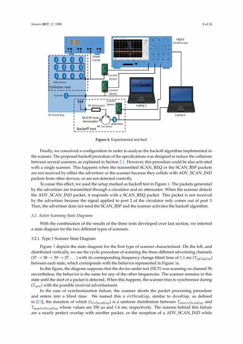
We performed three main tests in the scenario using the schema represented in Figure 4. First of all, we designed a collision test. In this case, we placed a scanner and up to 18 advertisers inside an RF-shield box. A laptop was employed to control the scanner and capture the Bluetooth Host Controller Interface (HCI) data using Tshark [16]. With this configuration, we fixed scanWindowT and

scanIntervalT to 500 ms to maintain a continuous active scanning. The advertisers were configured with the following parameters: advertising interval ( advIntervalT ), size of the advertising data ( advINDT ) and size of the scan response data ( scanRSPT ). The parameter values were set according to the evaluation conditions defined in Section 5. The experiment duration was 180 min for capturing packets with each of the different configurations. Then, we processed the raw data and calculated the non-detection probability of advertising and scan response packets and the time between consecutive detections among other statistics. Results will be presented later, combined with the ones of the analytical model and simulations.

Figure 4. Experimental test-bed.

Figure 3. Blind times due to non-idealities of real devices. (a) Type 1 scanners; (b) Type 2 scanners.

Now, the scannable undirected advertising mechanism is quite different from the non-connectableundirected advertising studied in our previous work. Bidirectional transmission, collision increaseand interference must be analyzed. On the other hand, the backoff algorithm needs to be characterized.We designed physical and MAC layer experimental measurements in order to understand the realbehavior of BLE devices and to obtain an accurate characterization. This characterization allows us toextend the analysis for a high number of devices and several parameter settings using simulationsand, additionally, to obtain an analytical model. Section 3.1 focuses on receiver measurements,which describe the real receiver baseband and MAC state characteristics of the Bluetooth devices,described in Section 3.2.

3.1. Measurement Setup Description

We performed three main tests in the scenario using the schema represented in Figure 4. First of all,we designed a collision test. In this case, we placed a scanner and up to 18 advertisers inside anRF-shield box. A laptop was employed to control the scanner and capture the Bluetooth Host ControllerInterface (HCI) data using Tshark [16]. With this configuration, we fixed TscanWindow and TscanInterval to500 ms to maintain a continuous active scanning. The advertisers were configured with the followingparameters: advertising interval (TadvInterval), size of the advertising data (TadvIND) and size of thescan response data (TscanRSP). The parameter values were set according to the evaluation conditionsdefined in Section 5. The experiment duration was 180 min for capturing packets with each ofthe different configurations. Then, we processed the raw data and calculated the non-detectionprobability of advertising and scan response packets and the time between consecutive detectionsamong other statistics. Results will be presented later, combined with the ones of the analytical modeland simulations.

Secondly, we designed a similar configuration to analyze the receiver behavior when it receivesscannable undirected advertising events. This is because when a packet is received, the scannermomentarily abandons the scanning state to process the packet; producing, in this way, differentpauses from those already analyzed. We characterized the behavior of the devices by simultaneouslymonitoring in an oscilloscope the instantaneous current consumption of the advertisers and the scannerusing current sensors, the design of which was based on [17]. As in [13], the aim was to analyze thecurrent consumption of the devices to extract behavior patterns of the scanner when it is receivingscannable undirected advertising events. However, in this case, we combined the information obtainedby behavior patterns with those obtained with Tshark. Thus, we were able to obtain information aboutsynchronization, packet detection, collision between ADV_SCAN_IND, SCAN_REQ and SCAN_RSPpackets, capture effects, etc. We processed the combined Tshark and the oscilloscope data in order toinfer a receiver state diagram.

Sensors 2017, 17, 1988 8 of 34

Sensors 2017, 17, 1988 7 of 34

settings using simulations and, additionally, to obtain an analytical model. Section 3.1 focuses on receiver measurements, which describe the real receiver baseband and MAC state characteristics of the Bluetooth devices, described in Section 3.2.

(a)

(b)

Figure 3. Blind times due to non-idealities of real devices. (a) Type 1 scanners; (b) Type 2 scanners.

3.1. Measurement Setup Description

We performed three main tests in the scenario using the schema represented in Figure 4. First of all, we designed a collision test. In this case, we placed a scanner and up to 18 advertisers inside an RF-shield box. A laptop was employed to control the scanner and capture the Bluetooth Host Controller Interface (HCI) data using Tshark [16]. With this configuration, we fixed scanWindowT and

scanIntervalT to 500 ms to maintain a continuous active scanning. The advertisers were configured with the following parameters: advertising interval ( advIntervalT ), size of the advertising data ( advINDT ) and size of the scan response data ( scanRSPT ). The parameter values were set according to the evaluation conditions defined in Section 5. The experiment duration was 180 min for capturing packets with each of the different configurations. Then, we processed the raw data and calculated the non-detection probability of advertising and scan response packets and the time between consecutive detections among other statistics. Results will be presented later, combined with the ones of the analytical model and simulations.

Figure 4. Experimental test-bed. Figure 4. Experimental test-bed.

Finally, we conceived a configuration in order to analyze the backoff algorithm implemented inthe scanner. The proposed backoff procedure of the specifications was designed to reduce the collisionsbetween several scanners, as explained in Section 2.1. However, this procedure could be also activatedwith a single scanner. This happens when the transmitted SCAN_REQ or the SCAN_RSP packetsare not received by either the advertiser or the scanner because they collide with ADV_SCAN_INDpackets from other devices, or are not detected correctly.

To cause this effect, we used the setup marked as backoff test in Figure 4. The packets generatedby the advertiser are transmitted through a circulator and an attenuator. When the scanner detectsthe ADV_SCAN_IND packet, it responds with a SCAN_REQ packet. This packet is not receivedby the advertiser because the signal applied to port 2 of the circulator only comes out of port 3.Then, the advertiser does not send the SCAN_RSP and the scanner activates the backoff algorithm.

3.2. Active Scanning State Diagrams

With the combination of the results of the three tests developed over last section, we inferreda state diagram for the two different types of scanners.

3.2.1. Type 1 Scanner State Diagram

Figure 5 depicts the state diagram for the first type of scanner characterized. On the left, anddistributed vertically, we see the cyclic procedure of scanning the three different advertising channels(37→ 38→ 39→ 37 . . . ) with its corresponding frequency change blind time of 1.1 ms (Tf qChgGap)between each state, which corresponds with the behavior represented in Figure 3a.

In this figure, the diagram supposes that the device under test (DUT) was scanning on channel 39;nevertheless, the behavior is the same for any of the other frequencies. The scanner remains in thisstate until the start of a packet is detected. When this happens, the scanner tries to synchronize during(Tsync) with the possible received advertisement.

In the case of synchronization failure, the scanner aborts the packet processing procedureand enters into a blind time. We named this a errDecodGap, similar to decodGap, as definedin [13], the duration of which (τerrDecodGap) is a uniform distribution between TminErrDecodGap andTmaxErrDecodGap whose values are 350 µs and 1.6 ms, respectively. The reasons behind this failureare a nearly perfect overlap with another packet, or the reception of a ADV_SCAN_IND while

Sensors 2017, 17, 1988 9 of 34

there a previous packet is still active from another device that did not initiate the decoding process.The receiver always tries to process the first packet received when coming from the scanning state.If the process has already been initiated when another packet is received, we confirmed that this secondpacket would always be discarded. If the synchronization is successful, the scanner waits for thecomplete reception of the ADV_SCAN_IND and checks its CRC. The CRC results in a failure in case ofpoor channel conditions or if the ADV_SCAN_IND collides with another PDU (ADV_SCAN_IND orADV_RSP). In this case, an errDecodGap is introduced.

Sensors 2017, 17, 1988 8 of 34

Secondly, we designed a similar configuration to analyze the receiver behavior when it receives scannable undirected advertising events. This is because when a packet is received, the scanner momentarily abandons the scanning state to process the packet; producing, in this way, different pauses from those already analyzed. We characterized the behavior of the devices by simultaneously monitoring in an oscilloscope the instantaneous current consumption of the advertisers and the scanner using current sensors, the design of which was based on [17]. As in [13], the aim was to analyze the current consumption of the devices to extract behavior patterns of the scanner when it is receiving scannable undirected advertising events. However, in this case, we combined the information obtained by behavior patterns with those obtained with Tshark. Thus, we were able to obtain information about synchronization, packet detection, collision between ADV_SCAN_IND, SCAN_REQ and SCAN_RSP packets, capture effects, etc. We processed the combined Tshark and the oscilloscope data in order to infer a receiver state diagram.

Finally, we conceived a configuration in order to analyze the backoff algorithm implemented in the scanner. The proposed backoff procedure of the specifications was designed to reduce the collisions between several scanners, as explained in Section 2.1. However, this procedure could be also activated with a single scanner. This happens when the transmitted SCAN_REQ or the SCAN_RSP packets are not received by either the advertiser or the scanner because they collide with ADV_SCAN_IND packets from other devices, or are not detected correctly.

To cause this effect, we used the setup marked as backoff test in Figure 4. The packets generated by the advertiser are transmitted through a circulator and an attenuator. When the scanner detects the ADV_SCAN_IND packet, it responds with a SCAN_REQ packet. This packet is not received by the advertiser because the signal applied to port 2 of the circulator only comes out of port 3. Then, the advertiser does not send the SCAN_RSP and the scanner activates the backoff algorithm.

3.2. Active Scanning State Diagrams

With the combination of the results of the three tests developed over last section, we inferred a state diagram for the two different types of scanners.

3.2.1. Type 1 Scanner State Diagram

Figure 5 depicts the state diagram for the first type of scanner characterized. On the left, and distributed vertically, we see the cyclic procedure of scanning the three different advertising channels (37 → 38 → 39 → 37 …) with its corresponding frequency change blind time of 1.1 ms ( fqChgGapT ) between each state, which corresponds with the behavior represented in Figure 3a.

Figure 5. Type 1 scanner state diagram. Figure 5. Type 1 scanner state diagram.

When the CRC check is passed, the scanner initiates the process of sending a SCAN_REQ.It waits for a TIFS, sends the SCAN_REQ, which has a duration of 176 µs, and waits for another TIFSbefore listening for the SCAN_RSP. If it does not detect any signal, it generates another blind time,with the same duration of the errDecodGap. On the contrary, it tries to synchronize with the receivedSCAN_RSP and checks its CRC in a similar way as done with the ADV_SCAN_IND. In this case,the scanner makes an errDecodGap when there is a failure on the synchronization. If the synchronizationis successful, it also introduces a decodGap after the CRC check no matter if it is successful or not.When successful, decodGap (τdecodGap) follows the same uniform distribution of τerrDecodGap. Whenthe CRC is successful, the scanner generates two HCI report events to the upper layer with thecontents of the ADV_SCAN_IND and SCAN_RSP received. In case of failure, the report only includesthe ADV_SCAN_IND.

As we have seen, the decodGap/errDecodGap is always introduced before returning to the scanningstate once the processing of a packet has been initiated. If a frequency change is scheduled withinthis process, it will be postponed until the start of the decodGap/errDecodGap. In this case, if thisdecodGap/errDecodGap and also the postponed Tf qChgGap occur simultaneously, the scanner only appliesthe largest of them.

Another important fact regarding this type of device is that we have verified that they do notimplement a backoff algorithm, although it is mandatory in the standard.

3.2.2. Type 2 Scanner State Diagram

Figure 6 depicts the state diagram for the second type of scanner characterized. In comparisonwith the state diagram for type 1 scanners, the state diagram in this case is somehow more complex.

Sensors 2017, 17, 1988 10 of 34Sensors 2017, 17, 1988 10 of 34

Figure 6. Type 2 scanner state diagram.

Another difference between the two device types is that, after a successful CRC check, type 2 devices apply the backoff algorithm described in Section 2.1. If the backoffCount is greater than one and, therefore, the SCAN_REQ is not sent, the scanner returns to the scanning state after introducing a blind time equal to the decodGap, with decodGap being constant and equal to 194 μs. In this case, an HCI report event with the contents of the ADV_SCAN_IND is generated to the upper layer. In contrast to Type 1, if a SCAN_REQ is to be transmitted, the device first checks if there is a periodic gap ( fqChgGapT or interFqChgGapT ) scheduled before the completion of the process. In these cases, the transmission of the SCAN_REQ is aborted. If a periodic gap is expected to be scheduled before a IFST, the scanner remains in a blind state for as much time as remains for the scheduled periodic gap. Finally, if a scheduled periodic gap was programmed between the end of the IFST and before the expected complete reception of the SCAN_RSP, the scanning device enters a blind time (waiting state) until the scheduled instant, and then introduces the periodic gap. From the point of view of the scanner, the expected duration of the SCAN_RSP will be the maximum allowed ( MAX

scanRSPT ); thus, the waiting time has a duration of up to scanREQ IFS

MAXscanRSPT TT .

Finally, when the SCAN_REQ is transmitted after a IFST , the scanner waits for the SCAN_RSP. If the synchronization is correct, an additional check is done to verify the packet type. If the received packet is another ADV_SCAN_IND, it returns to the point to check the CRC of the ADV_SCAN_IND. However, if the packet is the awaited SCAN_RSP, it checks its CRC. If this is successful, the scanning device introduces a decodGap and generates the corresponding two HCI report events to the upper layer, one for the ADV_SCAN_IND and one for the SCAN_RSP. If not, it only generates an HCI report event for the ADV_SCAN_IND and introduces an errDecodGap.

4. Analytical Model

In this section, we describe the mathematical model that allows us to characterize the BLE device discovery process. The model is derived according with the Bluetooth standard 5.0, but including the peculiarities of different implementations performed by the chipset manufacturers. We narrow our focus to deriving the performance metrics of the proposed interrupted version of the scannable undirected advertising event. This objective implies a previous characterization of the standard implementation of this same scheme without interruption. The final purpose is to compare both

Figure 6. Type 2 scanner state diagram.

The basic operation is similar; the scanner cycles over the three different frequencies in around-robin fashion with a small blind time between them (Tf qChgGap). In this case, this value isgreater than before, at 16.05 ms.

Additionally, to reproduce the behavior shown in Figure 3b, the scanner may exit now from thescanning state to introduce several TinterFqChgGap gaps, periodically. The details and specific values forthis behavior are described thoroughly in [13].

In a similar way to type 1 scanners, while the device is in any of the scanning states, once itstarts detecting energy on the channel, it begins packet processing. However, unlike the previouscase, now, when there is a failure in the synchronization or in the CRC check, the introduced gapwill be constant and considerably shorter than before (τerrDecodGap is 144 µs). Moreover, beforereturning to the scanning state, it is necessary to consider whether there was a postponed periodicgap (named a scheduled gap). In this case, the scheduled gaps may be not only the Tf qChgGap, but alsothe TinterFqChgGap.

Another difference between the two device types is that, after a successful CRC check, type 2devices apply the backoff algorithm described in Section 2.1. If the backoffCount is greater than one and,therefore, the SCAN_REQ is not sent, the scanner returns to the scanning state after introducing a blindtime equal to the decodGap, with τdecodGap being constant and equal to 194 µs. In this case, an HCIreport event with the contents of the ADV_SCAN_IND is generated to the upper layer. In contrast toType 1, if a SCAN_REQ is to be transmitted, the device first checks if there is a periodic gap (Tf qChgGapor TinterFqChgGap) scheduled before the completion of the process. In these cases, the transmission of theSCAN_REQ is aborted. If a periodic gap is expected to be scheduled before a TIFS, the scanner remainsin a blind state for as much time as remains for the scheduled periodic gap. Finally, if a scheduledperiodic gap was programmed between the end of the TIFS and before the expected complete receptionof the SCAN_RSP, the scanning device enters a blind time (waiting state) until the scheduled instant,and then introduces the periodic gap. From the point of view of the scanner, the expected duration ofthe SCAN_RSP will be the maximum allowed (TMAX

scanRSP); thus, the waiting time has a duration of up toTscanREQ + TIFS + TMAX

scanRSP.Finally, when the SCAN_REQ is transmitted after a TIFS, the scanner waits for the SCAN_RSP.

If the synchronization is correct, an additional check is done to verify the packet type. If the received

Sensors 2017, 17, 1988 11 of 34

packet is another ADV_SCAN_IND, it returns to the point to check the CRC of the ADV_SCAN_IND.However, if the packet is the awaited SCAN_RSP, it checks its CRC. If this is successful, the scanningdevice introduces a decodGap and generates the corresponding two HCI report events to the upperlayer, one for the ADV_SCAN_IND and one for the SCAN_RSP. If not, it only generates an HCI reportevent for the ADV_SCAN_IND and introduces an errDecodGap.

4. Analytical Model

In this section, we describe the mathematical model that allows us to characterize the BLE devicediscovery process. The model is derived according with the Bluetooth standard 5.0, but includingthe peculiarities of different implementations performed by the chipset manufacturers. We narrowour focus to deriving the performance metrics of the proposed interrupted version of the scannableundirected advertising event. This objective implies a previous characterization of the standardimplementation of this same scheme without interruption. The final purpose is to compareboth continuous and interrupted versions of the scannable undirected advertising event with thenon-connectable event with only advertising PDUs (previously studied in [13]).

The mathematical models developed here will be a useful instrument for effortlessly calculatingthe upper bounds of the discovery capacity, and for choosing the values of the parameter settings thatcontrol the advertising process, according to a particular BLE application. The two main configurationshave their own peculiarities that prevent them from using the same quantities, but there is a set ofparameters that allows the main capacities to be derived, and a fair comparison to be performed.The analytical models allow the characterization of the following parameters:

- Non-detection probabilities of ADV_SCAN_IND, SCAN_REQ and SCAN_RSP.- Mean discovery latency, associated with two possible parameters:

# Average ADV detection delay, defined as the time interval between the instant a BLE deviceenters advertising mode and the time instant when the ADV_SCAN_IND is successfullyreceived by the scanner.

# Average SCAN_REQ detection delay, defined as the time interval between the instanta BLE device enters advertising mode and the time instant when the SCAN_REQ issuccessfully received by the advertiser.

- Average time required for discovering all devices, defined as the time required for detecting allthe BLE devices in the coverage area.

- Probability that not all the BLE devices present in the scanner coverage area will be detectedwithin a limited time interval (window of opportunity or dwell time).

These parameters are in addition to:

- The mean time between consecutive ADV_SCAN_IND, SCAN_REQ or SCAN_RSP successfuldetections, associated to an advertising device.

- The mean number of ADV_SCAN_IND, SCAN_REQ or SCAN_RSP successful detections withina window of opportunity.

The mathematical characterization starts from the calculus of the collision probability betweenADV_SCAN_IND PDUs, assuming the ideal operation of BLE, in accordance with the standard(denoted as Pcol

NDAdvIND). Afterwards, we will employ it to obtain the overall ADV_SCAN_INDnon-detection probability (denoted as PNDAdvIND). In this case, the impairments of real BLE chipsetimplementations are included in the PNDAdvIND derivation, in accordance with characterizationsperformed in Section 3. PNDAdvIND will depend on several components: the collisions betweenADV_SCAN_IND packets from different advertisers, non-detections due to the scanner being involvedin the exchange of the following control messages (SCAN_REQ, SCAN_RSP) associated with the

Sensors 2017, 17, 1988 12 of 34

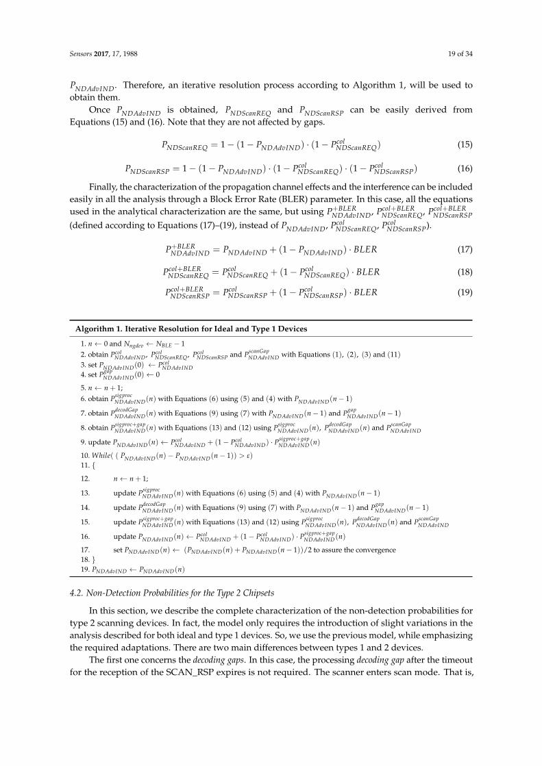
scanning procedure of another advertiser whose ADV_SCAN_IND has been successfully detected,preplanned scanning gaps identified in Section 3, post-processing decoding gaps and BLER (Block ErrorRate) due to interference, and noise and channel conditions. Subsequently, we calculate the SCAN_REQand SCAN_RSP non-detection probabilities, which in turn will condition the length of the time periodsin which the scanner is involved in the exchange of control messages during the scanning procedure.Consequently, they condition the probability of not detecting an ADV_SCAN_IND. The interrelationbetween the involved variables implies that the applied solution is iterative in several stages of theanalytical model.

Given the similarities between the ideal and type 1 scanning devices, we first model thenon-detection probabilities for these devices. Next, we include some variations to characterize thetype 2 scanning devices. Then, we obtain the main performance parameters used on the evaluationas the average time required to discover all the devices under the scanner coverage area. Finally,in Section 5, we will prove that the proposed mathematical model closely meets both the experimentaland simulation results obtained for a wide range of variation in the number of coexisting BLEadvertising devices.

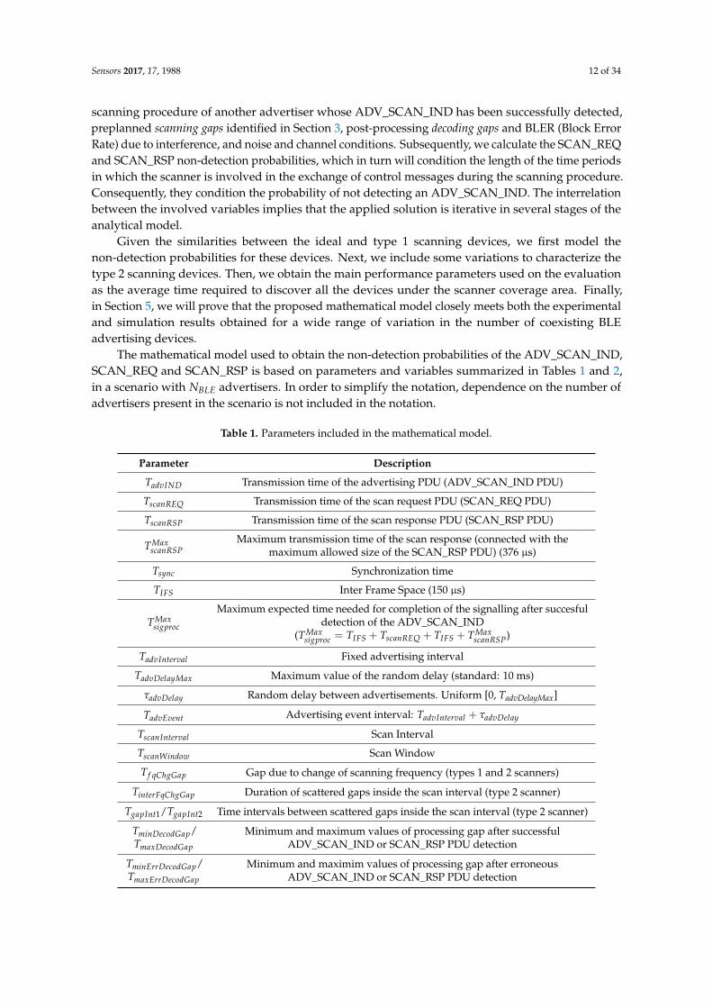
The mathematical model used to obtain the non-detection probabilities of the ADV_SCAN_IND,SCAN_REQ and SCAN_RSP is based on parameters and variables summarized in Tables 1 and 2,in a scenario with NBLE advertisers. In order to simplify the notation, dependence on the number ofadvertisers present in the scenario is not included in the notation.

Table 1. Parameters included in the mathematical model.

Parameter Description

TadvIND Transmission time of the advertising PDU (ADV_SCAN_IND PDU)

TscanREQ Transmission time of the scan request PDU (SCAN_REQ PDU)

TscanRSP Transmission time of the scan response PDU (SCAN_RSP PDU)

TMaxscanRSP

Maximum transmission time of the scan response (connected with themaximum allowed size of the SCAN_RSP PDU) (376 µs)

Tsync Synchronization time

TIFS Inter Frame Space (150 µs)

TMaxsigproc

Maximum expected time needed for completion of the signalling after succesfuldetection of the ADV_SCAN_IND

(TMaxsigproc = TIFS + TscanREQ + TIFS + TMax

scanRSP)

TadvInterval Fixed advertising interval

TadvDelayMax Maximum value of the random delay (standard: 10 ms)

τadvDelay Random delay between advertisements. Uniform [0, TadvDelayMax]

TadvEvent Advertising event interval: TadvInterval + τadvDelay

TscanInterval Scan Interval

TscanWindow Scan Window

Tf qChgGap Gap due to change of scanning frequency (types 1 and 2 scanners)

TinterFqChgGap Duration of scattered gaps inside the scan interval (type 2 scanner)

TgapInt1/TgapInt2 Time intervals between scattered gaps inside the scan interval (type 2 scanner)

TminDecodGap/TmaxDecodGap

Minimum and maximum values of processing gap after successfulADV_SCAN_IND or SCAN_RSP PDU detection

TminErrDecodGap/TmaxErrDecodGap

Minimum and maximim values of processing gap after erroneousADV_SCAN_IND or SCAN_RSP PDU detection

Sensors 2017, 17, 1988 13 of 34

Table 1. Cont.

Parameter Description

τdecodGapProcessing gap after successful ADV_SCAN_IND PDU or SCAN_RSP PDU

detection. Uniform [TminDecodGap,TmaxDecodGap]

τerrDecodGapProcessing gap after erroneus ADV_SCAN_IND PDU or SCAN_RSP PDU

detection. Uniform [TminErrDecodGap,TmaxErrDecodGap]

TscanGap Sum of durations of all the gaps occurred on the scan window

NscanWindowinterFqChgGap Number of scattered gaps inside the TscanWindow

Nngdev Number of neighbor advertising devices

NBLETotal number of advertising devices which are in the coverage area of the

scanning device and can potentially collide

Table 2. Variables included in the mathematical model (in a scenario with NBLE advertisers).

Variable Description

PpatternscanGap Probability that a periodic scanning gap occurs

RpatternscanGap Rate of periodic scanning

PMAXsigprocpatternscanGap Probability of having a periodic gap within TadvIND + TMAX

sigproc

NdetAdvINDMean number of neighbor devices whose ADV_SCAN_IND are detected

within TadvInterval + τadvDelay

PcolNDAdvIND

Non-detection probability (PND) of an ADV_SCAN_IND due to collision withanother ADV_SCAN_IND

PcolNDScanREQ * PND of a transmitted SCAN_REQ due to collision with an ADV_SCAN_IND

PcolNDScanRSP * PND of a transmitted SCAN_RSP due to collision with an ADV_SCAN_IND

TsigprocMean time the scanner is involved in a signaling processing period within a

TadvInterval + τadvDelay interval

PsigprocNDAdvIND

* PND of an ADV_SCAN_IND because the scanner is involved in asignaling processing period

TdecodGapMean time the scanner is involved in decoding gaps within a

TadvInterval + τadvDelay interval

PdecodGapNDAdvIND

* PND of an ADV_SCAN_IND because the scanner is involved in a decoding gap

PscanGapNDAdvIND

* PND of an ADV_SCAN_IND due to periodic scanning gaps

PgapNDAdvIND

* PND of an ADV_SCAN_IND due to scanning gaps(periodic scanning and decoding gaps)

Psigproc+gapNDAdvIND

* PND of an ADV_SCAN_IND due to scanning gaps andsignaling processing period

PNDAdvIND Overall * PND of a transmitted ADV_SCAN_IND

PNDScanREQ Overall * PND of a transmitted SCAN_REQ

PNdScanRSP Overall * PND of a transmitted SCAN_RSP

P+BLERNDAdvIND

Overall * PND of a transmitted ADV_SCAN_IND includingchannel errors (BLER)

Pcol+BLERNDScanREQ Overall * PND of a transmitted SCAN_REQ including channel errors (BLER)

Pcol+BLERNDScanRSP Overall * PND of a transmitted SCAN RSP including channel errors (BLER)

Sensors 2017, 17, 1988 14 of 34

Table 2. Cont.

Variable Description

PadvINDallDet

Probability of discover of all devices (based on ADV_SCAN_IND) withina DTH interval.

PscanREQallDet

Probability of discovering all devices (based on SCAN_REQ) withina DTH interval.

DadvINDallDet

Average time required to discover all devices based on ADV_SCAN_IND.

DscanREQallDet

Average time required to discover all devices based on SCAN_REQ

Nxpdureq

Average number of pdu (xpdu = ADV or SCAN_REQ) transmissions requiredbefore detection of a device

Dxpdudetect

Average detection delay of a pdu (xpdu = advIND or scanREQ)transmitted by a device

txpduinterDetect

Average time between two consecutive detections of a device(based on xpdu = advIND or scanREQ)

Nxpdudetect

Average number of detections of an advertiser BLE within a window ofopportunity (based on xpdu = advIND or scanREQ)

DTH Time threshold for detection

TcovWindow Coverage time interval or dwell time

* PND: non-detection probability.

As general considerations, we assume that NBLE + 1 devices are present in the scenario: a scannerdevice located in a fixed position plus NBLE advertisers that remain in coverage of the scanner duringa certain time period. As the objective is to discover the presence of a large number of devices in ashort time period, the scanner is configured to scan 100% of the time; that is, TscanInterval = TscanWindow .

A collision occurs when the PDU transmissions (ADV_SCAN_IND, SCAN_REQ or SCAN_RSP) ofat least two devices (scanner or advertisers) are time-overlapped on the same frequency channel.We assume that interference conditions are the same in the three available channels (37, 38, 39),and that all the advertiser devices are configured with the same parameter settings. Then, without lossof generality, we can characterize the non-detection probabilities assuming that both the scanner andthe advertisers are always scanning and transmitting, respectively, at the same frequency.

To derive the analytical model, the same assumption can be made for ideal and real devices:the starting time of the advertising event for a device in each channel is independent of each otherdevice, and is not affected by collisions or non-detections throughout the overall discovery process.Therefore, we can firstly obtain three preliminary non-detection probabilities that we will use as a basisfor the analytical models.

The collision probability between ADV_SCAN_IND PDUs in a scenario with NBLE advertisers isobtained with Equation (1). Note that, when setting a reference advertiser whose transmissionstarts at time instant t, a collision occurs with any other that initiates its transmission inthe time interval [t− TadvIND, t + TadvIND]. Given the time interval between consecutiveADV_SCAN_IND transmissions TadvInterval + τadvDelay, the collision probability between two devicesis 2 · TadvIND/(TadvInterval + τadvDelay). Transmissions of NBLE devices are independent; thus,the probability that the reference device collides with any of the other NBLE − 1 devices is one minusthe probability of not colliding with any of them. Note that collisions between ADV_SCAN_IND andSCAN_REQ or SCAN_RSP are not included in this variable.

PcolNDAdvIND = 1− (1− 2 · TadvIND

TadvEvent)

NBLE−1with TadvEvent = TadvInterval + τadvDelay (1)

Sensors 2017, 17, 1988 15 of 34

Once an ADV_SCAN_IND is detected by a scanner, the scanner is allowed to transmit a scanrequest to obtain additional information. In this case, the probability that the SCAN_REQ transmission(started in a time instant t) is not detected by the advertiser due to collision with an ADV_SCAN_INDtransmission from one of its neighbor devices depends on the probability that the ADV_SCAN_INDtransmission of another device starts in the time interval [t − min(TIFS, TadvIND), t + TscanREQ].However, note that a transmission that started in the interval [t− TadvIND, t− TIFS], given TadvIND > TIFS,would imply the non-detection of the ADV_SCAN_IND that is supposed to trigger the SCAN_REQresponse. Thus, this case is not possible. As TadvInterval + τadvDelay is the time interval betweenadvertisements transmissions, the probability of collision is (min(TIFS, TadvIND) + TscanREQ)/TadvEvent.In the same way that Pcol

NDAdvIND, the probability of collision between a SCAN_REQ and ADV_SCAN_INDtransmissions is given by Equation (2):

PcolNDScanREQ = 1− (1−

min(TIFS, TadvIND) + TscanREQ

TadvEvent)

NBLE−1

(2)

Following analogous considerations, Equation (3) characterizes the non-detection probability of aSCAN_RSP transmission caused by collisions with ADV_SCAN_IND transmissions from any other ofits neighbor devices. The non-detection probability of the SCAN_RSP transmission (started in a timeinstant t) due to collision with an ADV_SCAN_IND transmission from one of its neighbor devicesdepends on the probability that the ADV_SCAN_IND transmission of a neighbor device starts in theinterval [t−min(TIFS, TadvIND), t + TscanRSP]. As TadvInterval + τadvDelay is the time interval betweentransmitted advertisements, the collision probability is (min(TIFS, TadvIND) + TscanRSP)/TadvEvent.A transmission that started in the interval [t − TadvIND, t − TIFS], given TadvIND > TIFS, wouldimply the non-detection of the SCAN_REQ that is supposed to trigger the SCAN_RSP. Giventhat transmissions of the NBLE devices are independent, the SCAN_RSP collision probability withADV_SCAN_IND transmissions of other devices is one minus the probability of not colliding with anyof them.

PcolNDScanRSP = 1− (1− min(TIFS, TadvIND) + TscanRSP

TadvEvent)

NBLE−1

(3)

4.1. Non-Detection Probabilities for the Ideal and Type 1 Chipsets

Starting from the non-detection probabilities due to collisions included above, in this sectionwe describe a model that provides a complete characterization of the non-detection probabilities.The model includes the particularities of the scanning procedure with SCAN_REQ and SCAN_RSPPDUs, and also the behavior particularities of the manufactured BLE chipsets. In accordance withthe characterization performed in Section 3, the non-detection probability is affected by two types ofscanning pauses, which are included separately in the model. That is:

• The periodic scanning gaps. This kind of gap is always present. PscanGapNDAdvIND denotes the

non-detection probability of ADV_SCAN_IND due to these periods.• The decoding gaps. These gaps appear whenever the scanner decodes a packet or is unable to detect

an expected SCAN_RSP PDU after a specific timeout. Consequently, it depends on the numberof PDUs the scanner is detecting. That is, it really depends on the number of BLE advertisers inthe scanner coverage. PdecodGap

NDAdvIND denotes the non-detection probability of the ADV_SCAN_INDcaused by these blind times.

Ideal implementations according to the specification and type 1 real devices can be characterizedwith the same model, by only giving the value zero to the periodic scanning gaps and the decoding gapswhen the ideal case is considered. The main characteristic that allows this assumption is that periodicscanning gaps (which, in this case, are only associated with change frequency gaps) are prevented frominterrupting the general process. We have seen that, if an advertising event is initiated and, during theADV_SCAN_IND reception, the scanner has scheduled a periodic gap, this gap is postponed at least

Sensors 2017, 17, 1988 16 of 34

until the reception is finished (if synchronization is correct), regardless of whether the reception iscorrect or a collision or error occurs. Additionally, if the ADV_SCAN_IND reception is correct, or ifthe periodic scanning gap is planned to start once the ADV_SCAN_IND has been correctly received,the periodic gap is delayed up until the end of the SCAN_RSP reception or until the timeout on theSCAN_RSP reception is reached.

Derived from the PcolNDAdvIND, Pcol

NDScanREQ and PcolNDScanRSP probabilities, we first obtain the overall

non-detection probability of an ADV_SCAN_IND transmission (PNDAdvIND). We note that, in additionto collisions with other ADV_SCAN_IND (Pcol

NDAdvIND), an ADV_SCAN_IND transmission would beunable to be detected if the scanner were involved in the following events:

a. A signaling processing period. That is, the exchange of the following control messages associatedto the discovery procedure of another advertiser: SCAN_REQ, SCAN_RSP. In a scenario with NBLEadvertisers, two advertisers cannot simultaneously trigger the exchange of the control messages.However, in the time period between two consecutive advertisements from a “reference” device,the rest of the devices may trigger NBLE − 1, NBLE − 2, ..., one or no signaling processing gap onthe scanner, depending on the ADV_SCAN_IND non-detection probability. Consequently, we canobtain the mean time that the scanner is involved in a signaling processing period (Tsigproc) within aninterval TadvInterval + τadvDelay by multiplying the average time of these signaling processing periods(τsigproc) by the average number of devices that may generate it (NdetAdvIND). NdetAdvIND is obtainedaccording to Equation (4), given the number of neighbor advertising devices Nngdev = NBLE − 1.The population of advertising devices is finite, so the probability of having n signaling processingperiods follows a binomial distribution, which depends on the overall non-detection probability ofan ADV_SCAN_IND (PNDAdvIND). However, at the beginning of the iterative resolution process,PNDAdvIND is initialized by setting PNDAdvIND = Pcol

NDAdvIND.

NdetAdvIND =Nngdev

∑n=1

n · ( Nngdevn

)(1− PNDAdvIND)n · (PNDAdvIND)

(Nngdev)−n with Nngdev = NBLE − 1 (4)

Concerning the duration of the signaling processing period, the time interval needed to exchangecontrol messages always includes an interval TIFS + TScanREQ + TIFS and a variable time that dependson the successful transmission of the SCAN_REQ PDU (see Equation (5)). If the advertiser receivesthe SCAN_REQ PDU, it shall reply with a SCAN_RSP, but in the other case, after a timeout(synchronization time) without receiving the expected SCAN_RSP, the scanner moves to a decoding gap(type 1 real device) or to the scan mode. The ADV_SCAN_IND non-detection probability due to thesignaling processing periods (Psigproc

NDAdvIND) is the probability of generating an ADV_SCAN_IND withina signaling processing period or, as is the case in this situation, the probability that the scanner is in asignaling processing period (see Equation (6)).

τsigproc =[(TIFS + TscanREQ + TIFS) + (1− Pcol

NDScanREQ) · TscanRSP + PcolNDScanREQ · Tsync

](5)

PsigprocNDAdvIND =

Tsigproc

TadvInterval + τadvDelaywith Tsigproc = NdetAdvIND · τsigproc (6)

b. Decoding gaps. These scanning interruptions appear when the scanning device processesa detected ADV_SCAN_IND, a detected SCAN_RSP, or is unable to detect an expected SCAN_RSPPDU after a specific timeout. Decoding gaps are added to the signaling process gaps. In a similar wayto signaling processing gaps, the mean time that the scanner is involved in decoding gaps (TdecodGap)also depends on the mean number of neighbor devices that complete the signaling process withinan interval TadvInterval + τadvDelay. The mean time is the result of the sum of several gaps linked todifferent events: post-processing of a correct or erroneous SCAN_RSP transmission ((a) in Equation (7)),post-processing of a decoding gap (blind time) after the timeout for the reception of the SCAN_RSPexpires ((b) in Equation (7)), and post-processing of a decoding gap of an erroneous ADV_SCAN_IND

Sensors 2017, 17, 1988 17 of 34

transmission ((c) in Equation (7)). The characterization of the real chipset shows that an erroneousreception of the packet header, whose preamble has been detected, anticipates the trigger of a decodinggap. Thus, the analytical model considers both the gaps after the erroneous reception of the header partwith probability Tsync/TPDU , and the gaps after the complete reception of the PDU with probability(TPDU − Tsync)/TPDU (being TPDU equal to TadvIND or TscanRSP).

NdetAdvIND · (1− PcolNDScanREQ) ·

[(1− Pcol

NDScanRSP) · τdecodGap + PcolNDScanRSP · τerrDecodGap

∗]

with

τerrDecodGap∗ =

TscanRSP − Tsync

TscanRSP· τerrDecodGap +

Tsync

TscanRSP·max(0, (τerrDecodGap − (TscanRSP − Tsync)))

(7a)

+ NdetAdvIND · PcolNDScanREQ · τerrDecodGap (7b)

+(NBLE − 1− NdetAdvIND)

2·

PcolNDAdvIND · (1− Pgap

NDAdvIND)

PNDAdvIND· τerrDecodGap

∗∗ with

τerrDecodGap∗∗ =

TadvIND − Tsync

TadvIND· τerrDecodGap +

Tsync

TadvIND·max(0, (τerrDecodGap − (TadvIND − Tsync))) Being

(7c)

TdecodGap = Eq.7(a) + Eq.7(b) + Eq.7(c) (7d)

Concerning the average time that the scanner is involved in a decoding gap after the erroneousreception of an ADV_SCAN_IND, this is obtained by multiplying the average time of these decodinggaps (τerrDecodGap

∗) by the average number of BLE devices for whose signals synchronization hasbeen attempted, but which have not been detected due to a collision. That is, non-detected BLEdevices due to gaps (signaling processing, decoding or periodic) are not considered. On the otherhand, when a collision occurs, the scanner only tries to detect the preamble of the first arrivedPDU. This means that only one colliding ADV_SCAN_IND will potentially generate a decoding gap.In a simplified approach, if we assume that a collision involves two advertising devices, the meannumber of neighbor advertisers that are able to generate a decoding gap will be obtained by Equation (8).Note that (NBLE − 1− NdetAdvIND) is the number of neighbor advertisers whose ADV_SCAN_INDhave not been detected;

[Pcol

NDAdvIND · (1− PgapNDAdvIND)

]/PNDAdvIND, is the fraction of non-detections

due exclusively to collisions (PgapNDAdvIND, which will be introduced next). Finally, the product of the

two terms is divided by 2, because only one of the two advertisers involved in a collision generatesa decoding gap.

(NBLE − 1− NDetAdvIND)

2·

PcolNDAdvIND · (1− Pgap

NDAdvIND)

PNDAdvIND(8)

The ADV_SCAN_IND non-detection probability due to the decoding gaps (PdecodGapNDAdvIND) is the

probability of generating an ADV_SCAN_IND within a decoding gap period. This probability is equalto the probability that the scanner is in a decoding gap period, as is shown in Equation (9).

PdecodGapNDAdvIND =

TdecodGap

TadvInterval + τadvDelay(9)

c. Periodic scanning gaps. Assuming that there is only one scanning device, the probability ofthis type of gap (Ppattern

scanGap) is the quotient between the addition of the average durations of every

gap occurring in the scan window (denoted as TscanGap) and TscanWindow. PpatternscanGap is obtained by

Equation (10), given a number of gaps NscanWindowinterFqChgGap in a TscanWindow and derived by using TscanWindow,

Tf qChgGap , TinterFqChgGap, TgapInt1 and TgapInt2 parameters. This characterization is generic, and appliesfor both types 1 and 2 real devices.

PpatternscanGap =

TscanGap

TscanWindow=

Tf qChgGap + NscanWindowinterFqChgGap · TinterFqChgGap

TscanWindow(10)

Sensors 2017, 17, 1988 18 of 34

Once PpatternscanGap is derived, we need to clarify how periodic gaps affect the PDU’s detection. We have

seen that, once ADV_SCAN_IND reception is initiated, if the scanner has scheduled a periodic gap,two options can happen, with different results.

• Once a periodic gap is initiated, any transmission of ADV_SCAN_IND PDU that starts after thebeginning of the periodic gap cannot be detected. Then, the time intervals between successivegaps are not modified.

• If ADV_SCAN_IND PDU packet reception begins before the start time of a planned periodicgap, there are significant differences between chipsets from different manufacturers. When type 1scanner devices are evaluated, we measured that if an advertising event starts and the scannerhas scheduled a periodic gap during the ADV_SCAN_IND reception, this gap is postponed atleast until the reception is finished (no matter if the reception is correct or erroneous) or thedecoding gap is initiated (if the PDU header is erroneous). Additionally, if the ADV_SCAN_INDreception is correct, or if the periodic scanning gap is planned to start after the ADV_SCAN_INDhas been correctly received, the periodic gap is delayed until the end of the SCAN_RSP reception,or until the timeout on the SCAN_RSP reception is reached. It is clear that, in this situation,the interval from the delayed periodic gap and the following gap is shorter than the expectedones, in accordance with the pattern timing. Nevertheless, the following inter-gap intervalsremain unchanged.

Furthermore, it is known that, after erroneous ADV_SCAN_IND receptions, or after successfulSCAN_RSP receptions, the scanner introduces decoding gaps. In this case, the decoding gaps and alsothe delayed scanning gap should be planned to start simultaneously. Nevertheless, the largest of themis applied by the scanner. Furthermore, Ppattern

scanGap remains unchanged, in accordance with Equation (10).

Therefore, the ADV_SCAN_IND non-detection probability due to periodic scanning gaps (PscanGapNDAdvIND),

in accordance with Equation (11), is the probability of transmitting an ADV_SCAN_IND in the scanninggap interval, which is equal to Equation (9).

PscanGapNDAdvIND = Ppattern

scanGap =Tf qChgGap + NscanWindow

interFqChgGap · TinterFqChgGap

TscanWindow(11)

Once PscanGapNDAdvIND and PdecodGap

NDAdvIND are calculated, the probability that the scanner is in a scanninggap has to be derived, regardless of whether the scanning gap was a decoding gap or a periodic gap.As these two effects are considered to be independent, we use the Equation (12) to compute thenon-detection probability of ADV_SCAN_IND (Pgap

NDAdvIND) due to both effects.

PgapNDAdvIND = PscanGap

NDAdvIND + PdecodGapNDAdvIND − PscanGap

NDAdvIND · PdecodGapNDAdvIND (12)

Then, the ADV_SCAN_IND non-detection probability due to the scanning gaps must be added tothat due to the signaling processing period (see Equation (13)).

Psigproc+gapNDAdvIND = Psigproc

NDAdvIND + PgapNDAdvIND (13)

Finally, the ADV_SCAN_IND non-detection probability due to collisions and all the effectsexplained above can be obtained by Equation (14).

PNDAdvIND = PcolNDAdvIND + (1− Pcol

NDAdvIND) · Psigproc+gapNDAdvIND (14)

It is important to keep in mind that PsigprocNDAdvIND and PdecodGap

NDAdvIND components of Psigproc+gapNDAdvIND depend

on PNDAdvIND; and at the same time, PsigprocNDAdvIND, in addition to PdecodGap

NDAdvIND, will modify the probability

Sensors 2017, 17, 1988 19 of 34

PNDAdvIND. Therefore, an iterative resolution process according to Algorithm 1, will be used toobtain them.

Once PNDAdvIND is obtained, PNDScanREQ and PNDScanRSP can be easily derived fromEquations (15) and (16). Note that they are not affected by gaps.

PNDScanREQ = 1− (1− PNDAdvIND) · (1− PcolNDScanREQ) (15)

PNDScanRSP = 1− (1− PNDAdvIND) · (1− PcolNDScanREQ) · (1− Pcol

NDScanRSP) (16)

Finally, the characterization of the propagation channel effects and the interference can be includedeasily in all the analysis through a Block Error Rate (BLER) parameter. In this case, all the equationsused in the analytical characterization are the same, but using P+BLER

NDAdvIND, Pcol+BLERNDScanREQ, Pcol+BLER

NDScanRSP(defined according to Equations (17)–(19), instead of PNDAdvIND, Pcol

NDScanREQ, PcolNDScanRSP).

P+BLERNDAdvIND = PNDAdvIND + (1− PNDAdvIND) · BLER (17)

Pcol+BLERNDScanREQ = Pcol

NDScanREQ + (1− PcolNDScanREQ) · BLER (18)

Pcol+BLERNDScanRSP = Pcol

NDScanRSP + (1− PcolNDScanRSP) · BLER (19)

Algorithm 1. Iterative Resolution for Ideal and Type 1 Devices

1. n← 0 and Nngdev ← NBLE − 12. obtain Pcol

NDAdvIND , PcolNDScanREQ, Pcol

NDScanRSP and PscanGapNDAdvIND with Equations (1), (2), (3) and (11)

3. set PNDAdvIND(0) ← PcolNDAdvIND

4. set PgapNDAdvIND(0)← 0

5. n← n + 1;6. obtain Psigproc

NDAdvIND(n) with Equations (6) using (5) and (4) with PNDAdvIND(n− 1)

7. obtain PdecodGapNDAdvIND(n) with Equations (9) using (7) with PNDAdvIND(n− 1) and Pgap

NDAdvIND(n− 1)

8. obtain Psigproc+gapNDAdvIND(n) with Equations (13) and (12) using Psigproc

NDAdvIND(n), PdecodGapNDAdvIND(n) and PscanGap

NDAdvIND

9. update PNDAdvIND(n)← PcolNDAdvIND + (1− Pcol

NDAdvIND) · Psigproc+gapNDAdvIND(n)

10. While( ( PNDAdvIND(n)− PNDAdvIND(n− 1)) > ε)

11. {

12. n← n + 1;

13. update PsigprocNDAdvIND(n) with Equations (6) using (5) and (4) with PNDAdvIND(n− 1)

14. update PdecodGapNDAdvIND(n) with Equations (9) using (7) with PNDAdvIND(n− 1) and Pgap

NDAdvIND(n− 1)

15. update Psigproc+gapNDAdvIND(n) with Equations (13) and (12) using Psigproc

NDAdvIND(n), PdecodGapNDAdvIND(n) and PscanGap

NDAdvIND

16. update PNDAdvIND(n)← PcolNDAdvIND + (1− Pcol

NDAdvIND) · Psigproc+gapNDAdvIND(n)

17. set PNDAdvIND(n)← (PNDAdvIND(n) + PNDAdvIND(n− 1))/2 to assure the convergence18. }19. PNDAdvIND ← PNDAdvIND(n)

4.2. Non-Detection Probabilities for the Type 2 Chipsets

In this section, we describe the complete characterization of the non-detection probabilities fortype 2 scanning devices. In fact, the model only requires the introduction of slight variations in theanalysis described for both ideal and type 1 devices. So, we use the previous model, while emphasizingthe required adaptations. There are two main differences between types 1 and 2 devices.

The first one concerns the decoding gaps. In this case, the processing decoding gap after the timeoutfor the reception of the SCAN_RSP expires is not required. The scanner enters scan mode. That is,

Sensors 2017, 17, 1988 20 of 34

the mean time that the scanner is involved in decoding gaps (TdecodGap), used to compute the PdecodGapNDAdvIND

(Equation (20)) is equivalent to Equation (9), with the (a) and (c) components described in Equation (7).

TdecodGap = Eq.7(a) + Eq.7(c) (20)

The second difference is the impact of periodic scanning gaps. Contrary to type 1 scanning devices,if the ADV_SCAN_IND reception prior to the beginning of a periodic gap, it is necessary to includethe following cases:

The same as with type 1 scanning devices, if the scanner has planned to start a periodic gap duringthe ADV_SCAN_IND reception time, the pause is delayed at least up until the reception is finished(no matter whether the reception is correct or erroneous) or the decoding gap is initiated (when theheader part of the PDU is erroneous). However, if the scanner has planned to start a periodic gapduring the subsequent TIFS, the pause is delayed until the TIFS is finished and the discovery eventis closed in that frequency. The main difference occurs if the scanner has planned a periodic gap inthe time interval between the end of the first TIFS interval (between the ADV_SCAN_IND and theSCAN_REQ transmission) and the time the scanner expects to finish the reception of the SCAN_RSP.In this case, the scanner interrupts its operation until the time the periodic gap is planned, and thenexecutes the periodic gap. That is, the discovery event is closed. Note that, from the point of view ofthe scanner, the expected duration of the SCAN_RSP will be the maximum allowed (TMax

scanRSP).Assuming all that, we can conclude that any periodic gap planned along the maximum time

involving the discovery process (that is, TadvIND + TMaxsigproc, being TMax

sigproc = TIFS + TscanREQ + TIFS +

TMaxscanRSP) modifies the mean duration of the signaling processing period (Tsigproc).

In order to obtain Tsigproc, we firstly obtain the probability of having a periodic gap within the

TadvIND + TMaxsigproc (defined as PMaxSigproc

patternScanGap in Equation (22)) by multiplying the rate of periodic gaps

(RpatternscanGap), obtained by Equation (21), by TadvIND + TMax

sigproc.

RpatternscanGap =

1 + NscanWindowinterFqChgGap

TscanWindow(21)

PMaxSigprocpatternScanGap = Rpattern

scanGap · (TAdvIND + TMaxsigproc) (22)

Tsigproc is obtained by Equation (23), using τsigproc, as defined in Equation (5). Then, we derive

PsigprocNDAdvIND with Equation (24).

Tsigproc = NdetAdvIND ·[(1− PMaxSigproc

patternScanGap) · τsigproc + PMaxSigprocpatternScanGap · (TIFS +

(TscanREQ+TIFS+TMaxscanRSP)

2 )

](23)

PsigprocNDAdvIND =

Tsigproc

TadvInterval + τadvDelay(24)

Beyond the differences in the calculation of PsigprocNDAdvIND and PdecodGap

NDAdvIND, the process of computingPNDAdvIND is analogous to that used for ideal and type 1 scanning devices. In this case, the iterativeresolution process is rewritten in Algorithm 2.

Once PNDAdvIND is obtained, PNDScanREQ and PNDScanRSP can be easily derived fromEquations (25) and (26).

PNDScanREQ = 1− (1− PNDAdvIND) · (1− PcolNDScanREQ) · (1− PMaxSigproc

patternScanGap) (25)

PNDScanRSP = 1− (1− PNDAdvIND) · (1− PcolNDScanREQ) · (1− Pcol

NDScanRSP) · (1− PMaxSigprocpatternScanGap) (26)

Sensors 2017, 17, 1988 21 of 34

Finally, the effects of interference and channel response can be easily introduced in all the analysisthrough a BLER parameter, in a similar way to that described in Section 4.1.

Algorithm 2. Iterative Resolution for Type 2 Devices

1. n← 0 and Nngdev ← NBLE − 12. obtain Pcol

NDAdvIND , PcolNDScanREQ, Pcol

NDScanRSP, PscanGapNDAdvIND and PMaxSigproc

patternScanGapwith Equations (1), (2), (3), (11) and (22)3. set PNDAdvIND(0) ← Pcol

NDAdvIND

4. set PgapNDAdvIND(0)← 0

5. n← n + 1;6. obtain Psigproc

NDAdvIND(n) with Equations (24) using (23), (5) and (4) with PNDAdvIND(n− 1)

7. obtain PdecodGapNDAdvIND(n) with Equations (9) using (20) with PNDAdvIND(n− 1) and Pgap

NDAdvIND(n− 1)

8. obtain Psigproc+gapNDAdvIND(n) with Equations (13) and (12) using Psigproc

NDAdvIND(n), PdecodGapNDAdvIND(n) and PscanGap

NDAdvIND

9. update PNDAdvIND(n)← PcolNDAdvIND + (1− Pcol

NDAdvIND) · Psigproc+gapNDAdvIND(n)

10. While( ( PNDAdvIND(n)− PNDAdvIND(n− 1)) > ε)

11. {12. n← n + 1;13. update Psigproc

NDAdvIND(n) with Equations (24) using (23), (5) and (4) with PNDAdvIND(n− 1)

14. update PdecodGapNDAdvIND(n) with Equations (9) using (20) with PNDAdvIND(n− 1) and Pgap

NDAdvIND(n− 1)

15. update Psigproc+gapNDAdvIND(n) with Equations (13) and (12) using Psigproc

NDAdvIND(n), PdecodGapNDAdvIND(n) and PscanGap

NDAdvIND

16. update PNDAdvIND(n)← PcolNDAdvIND + (1− Pcol

NDAdvIND) · Psigproc+gapNDAdvIND(n)

17. set PNDAdvIND(n)← (PNDAdvIND(n) + PNDAdvIND(n− 1))/2 to assure the convergence18. }19. PNDAdvIND ← PNDAdvIND(n)

4.3. Derived Parameters of Interest

To compare both the standard and interrupted versions of the scannable undirected advertisingevent and non-connectable advertising event, with only advertising PDUs (named in the specificationsas ADV_NONCONN_IND and previously studied in [13]), the main parameters of interest are the

average time required to discover all devices based on SCAN_REQ detection (DscanREQallDet ) and the

average time required to discover all devices based on ADV_NONCONN_IND or in ADV_SCAN_IND

(DadvINDallDet ). The aim is that DscanREQ

allDet applies in scannable undirected advertising events, whereas

DadvINDallDet applies in non-connectable advertising events, with only advertising PDUs. Nevertheless,

the comparison is not fair, because when only ADV_NONCONN_IND are sent, the advertisers donot really know if they have been discovered. In order to perform a fairer comparison, assuming thatwe are really interested in knowing when the advertiser is aware of being discovered by the scanner,we can also obtain DadvIND

allDet for scannable undirected advertising events. In this case, this parameter iscalculated when the ADV_SCAN_IND is detected.

First, we can easily develop an approach for deriving the bound for DscanREQallDet , when advertisers

stop the discovery process once they have successfully received a SCAN_REQ. Detection delay forthe nth detected device depends on the PNDScanREQ probability, which changes over time, as neighbordevices are discovered and stop their advertising events. As an exact characterization makes theanalysis too complex for practical utility, we only derive a simple but accurate bound. The basis ofthe analysis, described in Algorithm 3, is simple. For each time interval between advertisementsof a reference advertiser (TadvInterval + TadvDelayMax), we assume that the number of undiscovereddevices in the system remains fixed. Starting from the number of devices present in the scenario(NBLE), we initialize the number of detected devices (NdevDet) to zero. Then, sequentially, wecompute PNDScanREQ according to the analytical models previously described. Once PNDScanREQ isobtained, we can derive the mean number of devices whose SCAN_REQ can be detected (NdetScanREQ)in each time interval. Note that the non-detection probabilities obtained in Sections 4.1 and 4.2

Sensors 2017, 17, 1988 22 of 34

implied a characterization of the mean number of detected devices in each advertising interval.Thus, the approach is adequate. Each round, we increase the number of detected devices (NdevDet)and decrease the number of neighbor devices (Nngdev) in the computed NdetScanREQ quantity, whilethe delay is increased by TadvInterval + TadvDelayMax. This process is repeated until only one deviceremains active. The last device is expected to generate a new advertisement with a mean delayof (TadvInterval + TadvDelayMax)/2. On the other hand, even if only one advertiser is present, themean time between the transmission of an advertising packet until the scanner correctly receives it,is tadvEvent · PNDScanREQ/(1− PNDScanREQ) .

Algorithm 3. Algorithm for Deriving the Bound for DscanREQallDet , When Advertisers Stop the Discovery

Process Once They Have Successfully Received a SCAN_REQ

1. set NdevDet ← 0, Ddet ← 0 and Nngdev ← NBLE − 1− NdevDet2. While( NdevDet < NBLE − 1)3. {4. obtain PNDAdvIND with Algorithm 1 or Algorithm 2 and Nngdev5. PNDScanREQ = 1− (1− PNDAdvIND) · (1− Pcol

NDScanREQ)

6. NdetScanREQ =Nngdev+1

∑i=1

i ·(

Nngdev + 1i

)(1− PNDScanREQ)

i · (PNDScanREQ)(Nngdev+1)−i

7. NdevDet ← NdevDet +⌊

NdetScanREQ⌋

8. Ddet ← Ddet + (TadvInterval + TadvDelayMax)

9. Nngdev ← NBLE − 1− NdevDet10. }11. obtain PNDScanREQ when NBLE = 1

12. DscanREQallDet ← Ddet +

(TadvInterval+TadvDelayMax)2 +

PNDScanREQ1−PNDScanREQ

· tadvEvent + (TadvIND + TIFS + TscanREQ)

Alternatively, and for comparison purposes, we can derive a bound for DscanREQallDet when the

advertisers do not stop the advertising process after they have been discovered. In this case(see Algorithm 4), each TadvInterval + TadvDelayMax interval, the number of devices that may be detectedis always the same. Thus, we only need to obtain the number of devices among the detected onesthat have not been previously discovered. The process can be applied to derive DadvIND

allDet by onlyconsidering PNDAdvIND and NdetAdvIND, instead of PNDScanREQ and NdetScanREQ.

We also have interest in deriving other parameters similar to those obtained for thenon-connectable advertising events, with only ADV_NONCONN_IND, previously characterizedin [13]. In order to introduce the parameters in a generalized form, they are referred to a generic xpdu,and must be replaced by advIND, scanREQ and scanRSP.

The average number of transmissions of a specific type of PDU (i.e., ADV_SCAN_IND, SCAN_REQ or

SCAN_RSP) required before detection (Nxpdureq ) can be straightforwardly obtained by Equation (27).

Nxpdureq = 1 · (1− PNDxpdu) +

∞

∑k=1

(1 + k) · (1− PNDxpdu) · PNDxpduk = 1 +

PNDxpdu

(1− PNDxpdu)(27)

We define the average detection delay (Dxpdudetect) as the mean time interval between the transmission

of the first xpdu (i.e., ADV_SCAN_IND, SCAN_REQ or SCAN_RSP) packet by the advertiser, and thecorrect reception of these xpdus correctly using Equation (28).

Dxpdudetect = (Nxpdu

req − 1) · tadvEvent (28)

Sensors 2017, 17, 1988 23 of 34

Using Equation (27), we can obtain the mean time between two consecutive detections withEquation (29).

txpduinterDetect = Nxpdu

req · tadvEvent (29)

Finally, the mean number of advertiser detections within a window of coverage, TcovWindow,or alternatively, a time threshold for detection under the coverage area, DTH (DTH < TcovWindow), is

Nxpdudetect =

min(DTH , TcovWindow)

txpduinterDetect

(30)

Algorithm 4. Algorithm for Deriving a Bound for DscanREQallDet When the Advertisers Do Not Stop the

Advertising Process After They Have Been Discovered

1. set NdevDet ← 0, , Ddet ← 0 and Nngdev ← NBLE − 12. obtain PNDAdvINDwith Algorithm 1 or Algorithm 2 and Nngdev3. PNDScanREQ = 1− (1− PNDAdvIND) · (1− Pcol

NDScanREQ)

4. NdetScanREQ =Nngdev+1

∑i=1

i · ( Nngdev + 1i

)(1− PNDScanREQ)i · (PNDScanREQ)

(Nngdev+1)−i

5. NdevDet ← NdevDet +⌊

NdetScanREQ⌋

6. Ddet ← Ddet + (TadvInterval + TadvDelayMax)

7. While (NdevDet < NBLE − 1)8. {9. PnewDevDet = 1− NdevDet/NBLE;

10. NnewDevDet =bNdetScanREQc

∑i=1

i · (⌊

NdetScanREQ⌋

i)(PnewDevDet)

i · (1− PnewDevDet)(bNdetScanREQc)−i

11. NdevDet ← NdevDet + NnewDevDet12. Ddet ← Ddet + (TadvInterval + TadvDelayMax)

13. }14. DscanREQ

allDet ← Ddet +(TadvInterval+TadvDelayMax)

2 +PNDScanREQ

1−PNDScanREQ· tadvEvent + (TadvIND + TIFS + TscanREQ)

5. Performance Evaluation

The device discovery process for BLE based on non-connectable advertising events with onlyadvertising PDUs is fairly simple. This is the reason why we explored the use of this process todiscover a high number of users in a short time period in [13]. This requirement concerns potentialapplications, such as the sport ones mentioned in Section 1. Scannable undirected advertising eventswere excluded in [13] due to the expected lower discovering capacities associated with higher signalingtraffic and, thus, their higher collision probabilities. However, the possibility of stopping the discoveryprocess after a successful detection of an SCAN_REQ makes this option more attractive in Bluetoothversion 5.0. Thus, in accordance with these potential applications requirements, we want to compareand quantify the discovery capacities for the three possible configurations: discovering processwith ADV_NONCONN_IND only, and continuous and interrupted processes with SCAN_REQ andSCAN_RSP. For evaluation purposes, the main parameters included in the analysis are:

• Non-detection probabilities of ADV_SCAN_IND (or alternatively ADV_NONCONN_IND),SCAN_REQ and SCAN_RSP, since they determine the overall non-detection probability andthey are involved in the determination of the average time required to discover all the devices

based on SCAN_REQ detection (DscanREQallDet ), and the average time required to discover all the

devices based on ADV_SCAN_IND detection (DadvINDallDet ).

Sensors 2017, 17, 1988 24 of 34

• The average time required to discover all the devices based on SCAN_REQ detection (DscanREQallDet )

and the average time required to discover all the devices based on ADV_SCAN_IND detection(DadvIND

allDet ) or ADV_NONCONN_IND detection.• Probability that all the devices are detected within a window of opportunity or a time threshold

for detection under the coverage area, DTH (DTH < TcovWindow).

The performance of the BLE discovery process, and particularly the tradeoff between discoverycapabilities versus energy consumption of the scanner, greatly depends on the selected scannerparameter settings (TscanInterval and TscanWindow values), in addition to the advertising interval and theadvertising PDU size. Once a scanning interval value is set in the scanner, its energy consumptiondecreases as long as the TscanWindow decreases, whereas the non-detection probability increases.Nevertheless, we have fixed TscanInterval = TscanWindow, because the goal is to detect the highestnumber of BLE devices in the shortest time interval. Firstly, the analysis, simulations and experimentsare done in almost ideal conditions. Experiments are configured in controlled conditions, withoutthe presence of interferences and low channel losses. After verifying that the simulation andthe mathematical model meet the results obtained in the experimental tests, both the model andthe simulation tool allow us to extend the analysis to a higher number of devices and severalchannel/interference conditions. Concerning the advertisers, in this section we analyze the impactof real peculiarities of the BLE chipsets on the discovery capacities, and the impact of TadvInterval andADV_NONCONN_IND/ADV_SCAN_IND PDUs sizes.

Results

We developed a simulator in C++ that fully reproduces (without any simplification) both theadvertising process in according with BLE specification and the real scanner configurations accordingto the peculiarities described Section 3. In order to obtain the performance statistics, we averagedup to 10,000 coverage time intervals. Errors due to interference or channel loss conditions canbe considered. However, to reproduce the experimental conditions, results are obtained in idealconditions (i.e., BLER = 0%). As mentioned above, the experimental testbed was configured incontrolled conditions to make these effects negligible. Specifically, the advertising BLEs transmit witha power level of 4 dBm. In a scenario with only one advertising BLE, we verified that with 4 dBm andwith a power transmission level of −40 dBm, the non-detection probability corresponds to PscanGap

NDAdvIND

and PscanGapNDScanRSP, respectively. Thus, the BLER effects are almost negligible and the assumption of

ideal conditions is suitable. In a real operating scenario, the time interval where an advertiser and thescanner are under mutual coverage may vary from one advertiser to another, as there may be timeswhen the link is obstructed by obstacles (for example, a runner may be obstructed by other runners).It is important that the scanner is placed in a position with a good view of the entire area to be covered.In addition, our study considered the worst-case scenario, in which any overlap between two receivedpackets results in the loss of both. In practice, there would be a capture effect, so that a good number ofcollisions would allow correct decoding of one of the packets. In any case, all this affects all discoverymethods, not only the one proposed in this paper, and in no way is our proposal more affected bythese situations. The most important parameters used in the evaluation are summarized in Table 3.

Figure 7 shows the non-detection probabilities of ADV_SCAN_IND (PNDAdvIND) and SCAN_RSP(PNDScanREQ), when a continuous scannable undirected advertising event involving SCAN_REQ andSCAN_RSP is considered. The aim was to compare the simulation results (Sim) and the mathematicalmodel results (Model), obtained when real scanning devices are assumed (types 1 and 2 scanningdevices are denoted as types 1 and 2, respectively), with the experimental measurement results(Exp), as the number of advertisers increases from 2 to 18. Results are obtained for TadvIND =

TscanREQ =176 µs, TscanRSP = 152 µs with TadvInterval = 100 ms and TadvDelayMax =10 ms. We can seethat the experimental results are in perfect agreement with the mathematical model and the simulations.Thus, we can assume that the scanner is well characterized, and the mathematical model is accurate.

Sensors 2017, 17, 1988 25 of 34

Note that the analytical model and both the simulation and experimental results for type 1 scanningdevices do not implement the backoff algorithm. Nevertheless, for type 2 scanning devices, Figure 7includes experimental and simulation results taking into account the backoff algorithm (denotedby B in theFigure 7), in addition to the results obtained by simulation and by the analytical modelwithout backoff implementation. We note that results are analogous because the backoff effect is almostnegligible when the number of devices involved in the scenario is low.

Table 3. Parameters used in the evaluation.

General Parameters Real Scanner Service Parameters

Parameter Values ParameterValues

Type 1 Type 2

TadvIND 176 µs, 376 µs Tf qChgGap 1.1 ms 16.04 ms

TadvInterval 100 ms, 500 ms TinterFqChgGap - 274 µs

TadvDelayMax 10 ms TgapInt1 - 16.82 ms

TscanInterval/TscanWindow 500 ms/500 ms TgapInt2 - 4.3 ms

TcovWindow/DTH 20 s/5 s TminDecodGap/TminErrDecodGap 350 ms/350 ms 194 µs/144 µs

NBLE 2–200 TmaxDecodGap/TmaxErrDecodGap 1.6 ms/1.6 ms 194 µs/144 µs

Sensors 2017, 17, 1988 26 of 34

the number of BLE advertisers is low. However, as shown in Figure 8, the weight of this effect decreases as the number of advertisers grows, and type 2 scanner is a better choice for these parameter settings when a large number of advertisers coexist.

Figure 7. ADV_SCAN_IND (ADV) and SCAN_RSP (RSP) non-detection probabilities for types 1 and 2 scanning devices and scannable undirected advertising, with backoff (denoted by B) and without backoff implementation. Comparison between experimental measurements (Exp), simulation (Sim) and the analytical model (Model) for advIND scanREQT T 176 μs, scanRSPT 152 μs

with advIntervalT 100 ms and advDelayMaxT 10 ms.

Figure 8 extends the comparison performed in Figure 7 for a higher number of advertisers, BLEN up to 200. ADV_SCAN_IND, SCAN_REQ and SCAN_RSP non-detection probabilities results, obtained by simulation, for the scannable undirected advertising with backoff (denoted by ADV/RSP/REQ Backoff) and without backoff implementation (denoted as ADV/RSP/REQ No backoff), are compared with the ADV_NONCONN_IND non-detection probability for non-connectable advertising events (denoted as NonConn). The comparison is performed for ideal (a), type 1 (b) and type 2 (c), assuming the same configuration ( advIND scanREQT T 176 μs, scanRSPT 152 μs with advIntervalT 100 ms and advDelayMaxT 10 ms). The analytical model results for scannable undirected advertising without backoff are also included. Firstly, we notice that the analytical model nearly matches with the results of the simulations for the whole range of devices when no backoff implementation is considered. If we narrow the focus of the analysis to scannable undirected advertising, it is evident that the differences between actual devices and the ideal implementation cannot be ignored. As already mentioned, for a higher number of advertisers, if no backoff implementation is considered, type 2 scanning devices offer better results than type 1 in terms of SCAN_REQ non-detection probabilities, even though this advantage is not as significant as when ADV_SCAN_IND is compared. If backoff implementation is included, we realize the negative and highly limiting impact of this mechanism in all cases. Note that, as we explained in Section 3, backoff is only present in type 2 scanning devices, but it has been included in type 1 devices for comparison purposes. In this case, SCAN_REQ and SCAN_RSP non-detection probabilities grow, because SCAN_REQ are actually prevented from being transmitted (collisions between PDUs grow and thus upperLimit of the backoff algorithm is doubled until it reaches its maximum, 256, on many occasions). Accordingly, ADV_SCAN_IND non-detection probabilities for the scannable undirected advertising converge to values similar to those obtained with non-connectable advertising events, as the number of SCAN_REQ tends to zero in scenarios with a high number of devices. The backoff mechanism is not really required in a scenario with only one scanner, but the mandatory implementation unnecessarily degrades the discovering capacities for a larger number of devices, if the SCAN_REQ

0

0.1

0.2

0.3

0.4

0.5

2 4 6 8 10 12 14 16 18

ADV Type 1 (Exp)ADV Type 1 (Sim)ADV Type 1 (Model)RSP Type 1 (Exp)RSP Type 1 (Sim)RSP Type 1 (Model)ADV Type 2 B (Exp)ADV Type 2 B (Sim)ADV Type 2 (Sim)ADV Type 2 (Model)RSP Type 2 B (Exp)RSP Type 2 B (Sim)RSP Type 2 (Sim)RSP Type 2 (Model)

Non

-det

ectio

n pr

obab

ility

Number of devices

Type 2 real devices (RSP)

Type 2 real devices (ADV)

Type 1 realdevices (ADV)

Type 1 realdevices (RSP)

Figure 7. ADV_SCAN_IND (ADV) and SCAN_RSP (RSP) non-detection probabilities for types 1and 2 scanning devices and scannable undirected advertising, with backoff (denoted by B) andwithout backoff implementation. Comparison between experimental measurements (Exp), simulation(Sim) and the analytical model (Model) for TadvIND = TscanREQ = 176 µs, TscanRSP = 152 µs withTadvInterval = 100 ms and TadvDelayMax = 10 ms.

By comparing the results of both ADV_SCAN_IND and SCAN_RSP non-detection probabilities,we can observe that differences between the actual implementations are quite significant and have tobe considered. In this case, and considering the ADV_SCAN_IND non-detection probability, the type 1scanner has a better performance than the type 2 up to eight advertisers, with the type 2 devicebeing better for higher values. Nevertheless, the advantages of the type 2 real device in terms ofADV_SCAN_IND non-detection probability are not maintained when SCAN_RSP is considered. As weexplained above, in type 2 scanning devices, if a periodic gap is planned between the reception ofthe ADV_SCAN_IND and the time the scanner expects to finish the reception of the SCAN_RSP,

Sensors 2017, 17, 1988 26 of 34

the scanner interrupts its operation until the time the periodic gap is planned, and then executes theperiodic gap. This results in higher SCAN_REQ and SCAN_RSP non-detection probabilities, when thenumber of BLE advertisers is low. However, as shown in Figure 8, the weight of this effect decreases asthe number of advertisers grows, and type 2 scanner is a better choice for these parameter settingswhen a large number of advertisers coexist.

Sensors 2017, 17, 1988 27 of 34

reception is considered as criterion. In fact, when backoff is used and the number of advertisers exceeds a value of about 100 (for the set of parameters defined), the discovering capacities of scannable undirected and non-connectable advertising event will be very similar, from a ADV_SCAN_IND or ADV_NONCONN_IND reception perspective. Nevertheless, the use of a scannable undirected advertising scheme makes no sense, given that it does not work as it should. Thus, potential enhancements could include better-adapted designs of the backoff process, or even deactivation under certain conditions. In the end, type 1 scanning devices, even though it seems that they do not meet the standard recommendations (i.e., do not implement backoff), offer the best results.

(a) Ideal

(b) Type 1 real devices

(c) Type 2 real devices

Figure 8. ADV_SCAN_IND (ADV), SCAN_REQ (REQ), SCAN_RSP (RSP) and ADV_NONCONN_IND (ADV NonConn) non-detection probabilities for scannable undirected and non-connectable advertising events, with and without backoff (denoted by Backoff and No Backoff) implementation, as the number of advertisers increases. Comparison between the mathematical model and the simulation for ideal (a), type 1 (b) and type 2 (c) scanning devices, for advIND scanREQT T

176 μs, scanRSPT 152 μs with advIntervalT 100 ms and advDelayMaxT 10 ms.

In any case, and as expected, if we compare the schemes only from the advertising packet non-detection probability perspective, it is clear that the standard continuous scannable undirected advertising offers lower discovery capacities than the non-connectable option. So, we extend the analysis to the proposed adapted version of scannable undirected advertising.

In order to do that, Figure 9 extends the comparison performed in Figure 8 to the average time required to discover all the devices based on SCAN_REQ for the scannable undirected advertising event and ADV_NONCONN_IND reception for non-connectable advertising event. The comparison is not fair, because SCAN_REQ reception is a criterion more restrictive than ADV_SCAN_IND reception, but we consider that the reception of SCAN_REQ is a valuable indicator in the new scheme. Once a SCAN_REQ has been received by an advertiser, we can be assured that both the advertiser and the scanner realize that the device has been discovered. If only ADV_SCAN_IND reception is used, the device has been discovered, but the advertiser is not aware. Now, simulation and analytical model results are obtained for the continuous advertising event with SCAN_REQ and SCAN_RSP, whereas only the simulation is shown for the schemes when the advertiser interrupts the advertising process (denoted as INT) after correctly receiving an SCAN_REQ and when non-connectable advertising events with only ADV_NONCONN_IND are considered. We see that the upper bound (derived analytically) for the average time required to discover all the devices closely matches the simulation results, both for the interrupted and continuous version of the scannable undirected advertising events. The backoff implementation has a severe impact on SCAN_REQ reception. For example, results show that the interrupted version without backoff clearly offers better results than the non-connectable advertising scheme, previously analyzed in [13], when real devices are considered, particularly for type 1 devices. In the ideal implementation, differences are almost negligible from the mean delay point of view. Thus, it is clear that real chipset implementation needs to be considered in any evaluation. Until now, the adapted scannable indirect scheme not only

0

0.2

0.4

0.6

0.8

1

0 50 100 150 200

ADV No Backoff (Sim)ADV No Backoff (Model)REQ No Backoff (Sim)REQ No Backoff (Model)RSP No Backoff (Sim)RSP No Backoff (Model)ADV Backoff (Sim)REQ Backoff (Sim)RSP Backoff (Sim)ADV NonConn (Sim)

Non

-det

ectio

n pr

obab

ility

Number of devices

Ideal devices

TadvIND=176sTadvInterval =100ms

0

0.2

0.4

0.6

0.8

1

0 50 100 150 200

ADV No Backoff (Sim)ADV No Backoff (Model)REQ No Backoff (Sim)REQ No Backoff (Model)RSP No Backoff (Sim)RSP No Backoff (Model)ADV Backoff (Sim)REQ Backoff (Sim)RSP Backoff (Sim)ADV NonConn (Sim)

Non

-det

ectio

n pr

obab

ility

Number of devices

Type 1 real devices

TadvIND=176sTadvInterval =100ms

0

0.2

0.4

0.6

0.8

1

0 50 100 150 200

ADV No Backoff (Sim)ADV No Backoff (Model)REQ No Backoff (Sim)REQ No Backoff (Model)RSP No Backoff (Sim)RSP No Backoff (Model)ADV Backoff (Sim)REQ Backoff (Sim)RSP Backoff (Sim)ADV NonConn (Sim)

Non

-det

ectio

n pr

obab

ility

Number of devices

Type 2 real devices

TadvIND=176sTadvInterval =100ms

Figure 8. ADV_SCAN_IND (ADV), SCAN_REQ (REQ), SCAN_RSP (RSP) and ADV_NONCONN_IND(ADV NonConn) non-detection probabilities for scannable undirected and non-connectable advertisingevents, with and without backoff (denoted by Backoff and No Backoff) implementation, as thenumber of advertisers increases. Comparison between the mathematical model and the simulation forideal (a), type 1 (b) and type 2 (c) scanning devices, for TadvIND = TscanREQ = 176 µs, TscanRSP = 152 µswith TadvInterval = 100 ms and TadvDelayMax = 10 ms.

Figure 8 extends the comparison performed in Figure 7 for a higher number of advertisers, NBLEup to 200. ADV_SCAN_IND, SCAN_REQ and SCAN_RSP non-detection probabilities results, obtainedby simulation, for the scannable undirected advertising with backoff (denoted by ADV/RSP/REQBackoff) and without backoff implementation (denoted as ADV/RSP/REQ No backoff), are comparedwith the ADV_NONCONN_IND non-detection probability for non-connectable advertising events(denoted as NonConn). The comparison is performed for ideal (a), type 1 (b) and type 2 (c), assumingthe same configuration (TadvIND = TscanREQ = 176 µs, TscanRSP = 152 µs with TadvInterval = 100 msand TadvDelayMax = 10 ms). The analytical model results for scannable undirected advertising withoutbackoff are also included. Firstly, we notice that the analytical model nearly matches with the resultsof the simulations for the whole range of devices when no backoff implementation is considered.If we narrow the focus of the analysis to scannable undirected advertising, it is evident that thedifferences between actual devices and the ideal implementation cannot be ignored. As alreadymentioned, for a higher number of advertisers, if no backoff implementation is considered, type 2scanning devices offer better results than type 1 in terms of SCAN_REQ non-detection probabilities,even though this advantage is not as significant as when ADV_SCAN_IND is compared. If backoffimplementation is included, we realize the negative and highly limiting impact of this mechanism inall cases. Note that, as we explained in Section 3, backoff is only present in type 2 scanning devices,but it has been included in type 1 devices for comparison purposes. In this case, SCAN_REQ andSCAN_RSP non-detection probabilities grow, because SCAN_REQ are actually prevented from beingtransmitted (collisions between PDUs grow and thus upperLimit of the backoff algorithm is doubleduntil it reaches its maximum, 256, on many occasions). Accordingly, ADV_SCAN_IND non-detectionprobabilities for the scannable undirected advertising converge to values similar to those obtainedwith non-connectable advertising events, as the number of SCAN_REQ tends to zero in scenarioswith a high number of devices. The backoff mechanism is not really required in a scenario with onlyone scanner, but the mandatory implementation unnecessarily degrades the discovering capacities fora larger number of devices, if the SCAN_REQ reception is considered as criterion. In fact, when backoff

Sensors 2017, 17, 1988 27 of 34

is used and the number of advertisers exceeds a value of about 100 (for the set of parameters defined),the discovering capacities of scannable undirected and non-connectable advertising event will be verysimilar, from a ADV_SCAN_IND or ADV_NONCONN_IND reception perspective. Nevertheless,the use of a scannable undirected advertising scheme makes no sense, given that it does not work as itshould. Thus, potential enhancements could include better-adapted designs of the backoff process,or even deactivation under certain conditions. In the end, type 1 scanning devices, even though itseems that they do not meet the standard recommendations (i.e., do not implement backoff), offer thebest results.

In any case, and as expected, if we compare the schemes only from the advertising packetnon-detection probability perspective, it is clear that the standard continuous scannable undirectedadvertising offers lower discovery capacities than the non-connectable option. So, we extend theanalysis to the proposed adapted version of scannable undirected advertising.

In order to do that, Figure 9 extends the comparison performed in Figure 8 to the average timerequired to discover all the devices based on SCAN_REQ for the scannable undirected advertisingevent and ADV_NONCONN_IND reception for non-connectable advertising event. The comparison isnot fair, because SCAN_REQ reception is a criterion more restrictive than ADV_SCAN_IND reception,but we consider that the reception of SCAN_REQ is a valuable indicator in the new scheme. Oncea SCAN_REQ has been received by an advertiser, we can be assured that both the advertiser andthe scanner realize that the device has been discovered. If only ADV_SCAN_IND reception is used,the device has been discovered, but the advertiser is not aware. Now, simulation and analytical modelresults are obtained for the continuous advertising event with SCAN_REQ and SCAN_RSP, whereasonly the simulation is shown for the schemes when the advertiser interrupts the advertising process(denoted as INT) after correctly receiving an SCAN_REQ and when non-connectable advertising eventswith only ADV_NONCONN_IND are considered. We see that the upper bound (derived analytically)for the average time required to discover all the devices closely matches the simulation results, both forthe interrupted and continuous version of the scannable undirected advertising events. The backoffimplementation has a severe impact on SCAN_REQ reception. For example, results show that theinterrupted version without backoff clearly offers better results than the non-connectable advertisingscheme, previously analyzed in [13], when real devices are considered, particularly for type 1 devices.In the ideal implementation, differences are almost negligible from the mean delay point of view.Thus, it is clear that real chipset implementation needs to be considered in any evaluation. Untilnow, the adapted scannable indirect scheme not only reduces the time required but also the energyconsumption of advertisers. On the other hand, advertisers are aware that they have been discovered.

The same analysis, based on a fairer discovery indicator (the ADV_SCAN_IND orADV_NONCONN_IND) reception for both scannable undirected and non-connectable advertisingevents) is performed in Figure 10. We see that the interrupted version without backoff clearly offersthe best results in all cases, with type 2 devices (without backoff) being the more attractive option.On the other hand, although we have excluded the backoff implementation, the interrupted versionwith backoff offers similar results to non-connectable advertising events for scenarios with a veryhigh number of devices. Nevertheless, in order to compare the proposals, not only the average timerequired to discover all the devices, but also the distribution, is important. Therefore, we compute theprobability that not all the devices are detected before a time threshold (DTH). Note that discoverycapacity depends on DTH , so it should be evaluated for each desired application by considering theappropriate value for DTH .

Figure 11, connected with the analysis performed in Figure 9, shows the probability of notdetecting all the advertising devices and aware of being detected by the scanner (in scannableundirected advertising schemes) when DTH is set to 5 s. Note that, when only ADV_NONCONN_INDand type 1 real devices are considered, the probability of not detecting all the advertisers whenNBLE = 200 is around 0.1%, whereas in the interrupted version all devices are detected when ideal,types 1 and 2 scanning devices are considered. On the other hand, if ADV_SCAN_IND is used

Sensors 2017, 17, 1988 28 of 34

as the detection indicator in the interrupted version of the scannable undirected advertising event,the probability that all the devices are detected is 100%.

Sensors 2017, 17, 1988 28 of 34

reduces the time required but also the energy consumption of advertisers. On the other hand, advertisers are aware that they have been discovered.

(a) Ideal (b) Type 1 real devices

(c) Type 2 real devices

Figure 9. Average time required to discover all devices (in seconds), based on ADV_NONCONN_IND (ADV NonConn) for non-connectable advertising events and SCAN_REQ (REQ) reception for scannable undirected advertising events (standard and interrupted versions) with and without backoff, as the number of advertisers increases. Comparison between the mathematical model and the simulation for ideal (a), type 1 (b) and type 2 (c) scanning devices, for advIND scanREQT T

176 μs, scanRSPT 152 μs with advIntervalT 100 ms and advDelayMaxT 10 ms.

The same analysis, based on a fairer discovery indicator (the ADV_SCAN_IND or ADV_NONCONN_IND) reception for both scannable undirected and non-connectable advertising events) is performed in Figure 10. We see that the interrupted version without backoff clearly offers the best results in all cases, with type 2 devices (without backoff) being the more attractive option. On the other hand, although we have excluded the backoff implementation, the interrupted version with backoff offers similar results to non-connectable advertising events for scenarios with a very high number of devices. Nevertheless, in order to compare the proposals, not only the average time required to discover all the devices, but also the distribution, is important. Therefore, we compute the probability that not all the devices are detected before a time threshold ( THD ). Note that discovery capacity depends on THD , so it should be evaluated for each desired application by considering the appropriate value for THD .

(a) Ideal (b) Type 1 real devices

(c) Type 2 real devices

Figure 10. Average time required to discover all devices (in seconds), based on ADV_SCAN_IND (ADV) reception for scannable undirected (standard and interrupted versions) and non-connectable advertising events ADV_NONCONN_IND (ADV NonConn), with and without backoff, as the number of advertisers increases. Comparison between ideal (a), type 1 (b) and type 2 (c) scanning devices, for advIND scanREQT T 176 μs, scanRSPT 152 μs with advIntervalT 100 ms and advDelayMaxT

10 ms.

Figure 11, connected with the analysis performed in Figure 9, shows the probability of not detecting all the advertising devices and aware of being detected by the scanner (in scannable

0

1

2

3

4

5

6

0 50 100 150 200

REQ No Backoff (Sim)REQ No Backoff (Model)REQ INT_No Backoff (Sim)REQ INT_No Backoff (Model)REQ Backoff (Sim)REQ INT_Backoff (Sim)ADV without REQ/RSP (Sim)

Number of devices

TadvIND=176sTadvInterval =100ms

Ideal devices

Aver

age

time

requ

ired

to d

isco

ver a

ll de

vice

s (s

)

REQ No Backoff (Sim)REQ No Backoff (Model)REQ INT_No Backoff (Sim)REQ INT_No Backoff (Model)REQ Backoff (Sim)REQ INT_Backoff (Sim)ADV NonConn Sim)

REQ No Backoff (Sim)REQ No Backoff (Model)REQ INT_No Backoff (Sim)REQ INT_No Backoff (Model)REQ Backoff (Sim)REQ INT_Backoff (Sim)ADV NonConn (Sim)

0

1

2

3

4

5

6

0 50 100 150 200Number of devices

Aver

age

time

requ

ired

to d

isco

ver a

ll de

vice

s (s

)

REQ No Backoff (Sim)REQ No Backoff (Model)REQ INT_No Backoff (Sim)REQ INT_No Backoff (Model)REQ Backoff (Sim)REQ INT_Backoff (Sim)ADV NonCon (Sim)

TadvIND=176sTadvInterval =100ms

Type 1 real devices

REQ No Backoff (Sim)REQ No Backoff (Model)REQ INT_No Backoff (Sim)REQ INT_No Backoff (Model)REQ Backoff (Sim)REQ INT_Backoff (Sim)ADV NonConn Sim)

REQ No Backoff (Sim)REQ No Backoff (Model)REQ INT_No Backoff (Sim)REQ INT_No Backoff (Model)REQ Backoff (Sim)REQ INT_Backoff (Sim)ADV NonConn (Sim)

0

1

2

3

4

5

6

0 50 100 150 200

REQ No Backoff (Sim)REQ No Backoff (Model)REQ INT_No Backoff (Sim)REQ INT_No Backoff (Model)REQ Backoff (Sim)REQ INT_Backoff (Sim)ADV without REQ/RSP (Sim)

Number of devices

TadvIND=176sTadvInterval =100ms

Type 2 real devices

Aver

age

time

requ

ired

to d

isco

ver a

ll de

vice

s (s

)

REQ No Backoff (Sim)REQ No Backoff (Model)REQ INT_No Backoff (Sim)REQ INT_No Backoff (Model)REQ Backoff (Sim)REQ INT_Backoff (Sim)ADV NonConn Sim)

REQ No Backoff (Sim)REQ No Backoff (Model)REQ INT_No Backoff (Sim)REQ INT_No Backoff (Model)REQ Backoff (Sim)REQ INT_Backoff (Sim)ADV NonConn (Sim)

0

0.5

1

1.5

2

0 50 100 150 200

ADV No Backoff (Sim)ADV INT_No Backoff (Sim)ADV Backoff (Sim)ADV INT_Backoff (Sim)ADV NonConn (Sim)

Ideal devices

TadvIND=176sTadvInterval =100ms

Number of devices

Aver

age

time

requ

ired

to d

isco

ver a

ll de

vice

s (s

)

0

0.5

1

1.5

2

2.5

3

3.5

0 50 100 150 200

ADV No Backoff (Sim)ADV INT_No Backoff (Sim)ADV Backoff (Sim)ADV INT_Backoff (Sim)ADV NonConn (Sim)

Type 1 real devices

TadvIND=176sTadvInterval =100ms

Number of devices

Aver

age

time

requ

ired

to d

isco

ver a

ll de

vice

s (s

)

0

0.5

1

1.5

2

0 50 100 150 200

ADV No Backoff (Sim)ADV INT_No Backoff (Sim)ADV Backoff (Sim)ADV INT_Backoff (Sim)ADV NonConn (Sim)

Type 2 real devices

TadvIND=176sTadvInterval =100ms

Number of devices

Aver

age

time

requ

ired

to d

isco

ver a

ll de

vice

s (s

)

Figure 9. Average time required to discover all devices (in seconds), based on ADV_NONCONN_IND(ADV NonConn) for non-connectable advertising events and SCAN_REQ (REQ) reception for scannableundirected advertising events (standard and interrupted versions) with and without backoff, as thenumber of advertisers increases. Comparison between the mathematical model and the simulation forideal (a), type 1 (b) and type 2 (c) scanning devices, for TadvIND = TscanREQ = 176 µs, TscanRSP = 152 µswith TadvInterval = 100 ms and TadvDelayMax = 10 ms.

Sensors 2017, 17, 1988 28 of 34

reduces the time required but also the energy consumption of advertisers. On the other hand, advertisers are aware that they have been discovered.

(a) Ideal (b) Type 1 real devices

(c) Type 2 real devices

Figure 9. Average time required to discover all devices (in seconds), based on ADV_NONCONN_IND (ADV NonConn) for non-connectable advertising events and SCAN_REQ (REQ) reception for scannable undirected advertising events (standard and interrupted versions) with and without backoff, as the number of advertisers increases. Comparison between the mathematical model and the simulation for ideal (a), type 1 (b) and type 2 (c) scanning devices, for advIND scanREQT T

176 μs, scanRSPT 152 μs with advIntervalT 100 ms and advDelayMaxT 10 ms.

The same analysis, based on a fairer discovery indicator (the ADV_SCAN_IND or ADV_NONCONN_IND) reception for both scannable undirected and non-connectable advertising events) is performed in Figure 10. We see that the interrupted version without backoff clearly offers the best results in all cases, with type 2 devices (without backoff) being the more attractive option. On the other hand, although we have excluded the backoff implementation, the interrupted version with backoff offers similar results to non-connectable advertising events for scenarios with a very high number of devices. Nevertheless, in order to compare the proposals, not only the average time required to discover all the devices, but also the distribution, is important. Therefore, we compute the probability that not all the devices are detected before a time threshold ( THD ). Note that discovery capacity depends on THD , so it should be evaluated for each desired application by considering the appropriate value for THD .

(a) Ideal (b) Type 1 real devices

(c) Type 2 real devices

Figure 10. Average time required to discover all devices (in seconds), based on ADV_SCAN_IND (ADV) reception for scannable undirected (standard and interrupted versions) and non-connectable advertising events ADV_NONCONN_IND (ADV NonConn), with and without backoff, as the number of advertisers increases. Comparison between ideal (a), type 1 (b) and type 2 (c) scanning devices, for advIND scanREQT T 176 μs, scanRSPT 152 μs with advIntervalT 100 ms and advDelayMaxT

10 ms.

Figure 11, connected with the analysis performed in Figure 9, shows the probability of not detecting all the advertising devices and aware of being detected by the scanner (in scannable

0

1

2

3

4

5

6

0 50 100 150 200

REQ No Backoff (Sim)REQ No Backoff (Model)REQ INT_No Backoff (Sim)REQ INT_No Backoff (Model)REQ Backoff (Sim)REQ INT_Backoff (Sim)ADV without REQ/RSP (Sim)

Number of devices

TadvIND=176sTadvInterval =100ms

Ideal devices

Aver

age

time

requ

ired

to d

isco

ver a

ll de

vice

s (s

)

REQ No Backoff (Sim)REQ No Backoff (Model)REQ INT_No Backoff (Sim)REQ INT_No Backoff (Model)REQ Backoff (Sim)REQ INT_Backoff (Sim)ADV NonConn Sim)

REQ No Backoff (Sim)REQ No Backoff (Model)REQ INT_No Backoff (Sim)REQ INT_No Backoff (Model)REQ Backoff (Sim)REQ INT_Backoff (Sim)ADV NonConn (Sim)

0

1

2

3

4

5

6

0 50 100 150 200Number of devices

Aver

age

time

requ

ired

to d

isco

ver a

ll de

vice

s (s

)

REQ No Backoff (Sim)REQ No Backoff (Model)REQ INT_No Backoff (Sim)REQ INT_No Backoff (Model)REQ Backoff (Sim)REQ INT_Backoff (Sim)ADV NonCon (Sim)

TadvIND=176sTadvInterval =100ms

Type 1 real devices

REQ No Backoff (Sim)REQ No Backoff (Model)REQ INT_No Backoff (Sim)REQ INT_No Backoff (Model)REQ Backoff (Sim)REQ INT_Backoff (Sim)ADV NonConn Sim)

REQ No Backoff (Sim)REQ No Backoff (Model)REQ INT_No Backoff (Sim)REQ INT_No Backoff (Model)REQ Backoff (Sim)REQ INT_Backoff (Sim)ADV NonConn (Sim)

0

1

2

3

4

5

6

0 50 100 150 200

REQ No Backoff (Sim)REQ No Backoff (Model)REQ INT_No Backoff (Sim)REQ INT_No Backoff (Model)REQ Backoff (Sim)REQ INT_Backoff (Sim)ADV without REQ/RSP (Sim)

Number of devices

TadvIND=176sTadvInterval =100ms

Type 2 real devices

Aver

age

time

requ

ired

to d

isco

ver a

ll de

vice

s (s

)

REQ No Backoff (Sim)REQ No Backoff (Model)REQ INT_No Backoff (Sim)REQ INT_No Backoff (Model)REQ Backoff (Sim)REQ INT_Backoff (Sim)ADV NonConn Sim)

REQ No Backoff (Sim)REQ No Backoff (Model)REQ INT_No Backoff (Sim)REQ INT_No Backoff (Model)REQ Backoff (Sim)REQ INT_Backoff (Sim)ADV NonConn (Sim)

0

0.5

1

1.5

2

0 50 100 150 200

ADV No Backoff (Sim)ADV INT_No Backoff (Sim)ADV Backoff (Sim)ADV INT_Backoff (Sim)ADV NonConn (Sim)

Ideal devices

TadvIND=176sTadvInterval =100ms

Number of devices

Aver

age

time

requ

ired

to d

isco

ver a

ll de

vice

s (s

)

0

0.5

1

1.5

2

2.5

3

3.5

0 50 100 150 200

ADV No Backoff (Sim)ADV INT_No Backoff (Sim)ADV Backoff (Sim)ADV INT_Backoff (Sim)ADV NonConn (Sim)

Type 1 real devices

TadvIND=176sTadvInterval =100ms

Number of devices

Aver

age

time

requ

ired

to d

isco

ver a

ll de

vice

s (s

)

0

0.5

1

1.5

2

0 50 100 150 200

ADV No Backoff (Sim)ADV INT_No Backoff (Sim)ADV Backoff (Sim)ADV INT_Backoff (Sim)ADV NonConn (Sim)

Type 2 real devices

TadvIND=176sTadvInterval =100ms

Number of devices

Aver

age

time

requ

ired

to d

isco

ver a

ll de

vice

s (s

)

Figure 10. Average time required to discover all devices (in seconds), based on ADV_SCAN_IND(ADV) reception for scannable undirected (standard and interrupted versions) and non-connectableadvertising events ADV_NONCONN_IND (ADV NonConn), with and without backoff, as thenumber of advertisers increases. Comparison between ideal (a), type 1 (b) and type 2 (c) scanningdevices, for TadvIND = TscanREQ = 176 µs, TscanRSP = 152 µs with TadvInterval = 100 ms andTadvDelayMax = 10 ms.

In order to better illustrate the analysis and the differences for the two more attractive options(the interrupted version of the scannable undirected advertising events and the non-connectableadvertising scheme), Figure 12 depicts the cumulative density function (CDF) of the time requiredto discover all the devices when NBLE = 200 advertisers are considered. We can see that the varianceis higher when the non-connectable advertising scheme is considered. In fact, as a more restrictivevalue for DTH is considered, the higher the advantages of the interrupted version are. For instance,if DTH is set to 2 s, none of devices are discovered when a type 1 scanning device is considered in anon-connectable advertising scheme, compared to 90% if a type 2 scanning device is used. For its part,the interrupted version guarantees that all the devices are discovered, regardless of whether ideal,type 1 or type 2 scanning devices are considered.

Sensors 2017, 17, 1988 29 of 34

Sensors 2017, 17, 1988 29 of 34

undirected advertising schemes) when THD is set to 5 s. Note that, when only ADV_NONCONN_IND and type 1 real devices are considered, the probability of not detecting all the advertisers when 200BLEN is around 0.1%, whereas in the interrupted version all devices are detected when ideal, types 1 and 2 scanning devices are considered. On the other hand, if ADV_SCAN_IND is used as the detection indicator in the interrupted version of the scannable undirected advertising event, the probability that all the devices are detected is 100%.

(a) Ideal (b) Type 1 real devices (c) Type 2 real devices

Figure 11. Probability that all devices are detected in THD ( 5THD s ), based on ADV_NONCONN_IND (ADV NonConn) for non-connectable advertising events and SCAN_REQ (REQ) reception for scannable undirected advertising events (standard and interrupted versions) with and without backoff, as the number of advertisers increases. Comparison between ideal (a), type 1 (b) and type 2 (c) scanning devices, for advIND scanREQT T 176 μs, scanRSPT 152 μs with

advIntervalT 100 ms and advDelayMaxT 10 ms.

In order to better illustrate the analysis and the differences for the two more attractive options (the interrupted version of the scannable undirected advertising events and the non-connectable advertising scheme), Figure 12 depicts the cumulative density function (CDF) of the time required to discover all the devices when 200BLEN advertisers are considered. We can see that the variance is higher when the non-connectable advertising scheme is considered. In fact, as a more restrictive value for THD is considered, the higher the advantages of the interrupted version are. For instance, if THD is set to 2 s, none of devices are discovered when a type 1 scanning device is considered in a non-connectable advertising scheme, compared to 90% if a type 2 scanning device is used. For its part, the interrupted version guarantees that all the devices are discovered, regardless of whether ideal, type 1 or type 2 scanning devices are considered.

Figure 12. CDF of the time required to discover all the devices when there are 200BLEN BLE advertisers for advIND scanREQT T 176 μs, scanRSPT 152 μs with advIntervalT 100 ms and

advDelayMaxT 10 ms. Comparison between the interrupted version of scannable undirected advertising

0.2

0.4

0.6

0.8

1

0 50 100 150 200

REQ No Backoff (Sim)REQ INT_No Backoff (Sim)REQ Backoff (Sim)REQ INT_Backoff (Sim)ADV NonConn (Sim)

Prob

abilit

y th

at a

ll de

vice

s a

re d

etec

ted

in D

TH

Ideal devices

TadvIND=176sTadvInterval =100ms

Number of devices

0.2

0.4

0.6

0.8

1

0 50 100 150 200

REQ No Backoff (Sim)REQ INT_No Backoff (Sim)REQ Backoff (Sim)REQ INT_Backoff (Sim)ADV NonConn (Sim)

Prob

abilit

y th

at a

ll de

vice

s a

re d

etec

ted

in D

TH

Type 1 real devices

Number of devices

TadvIND=176sTadvInterval =100ms

0.2

0.4

0.6

0.8

1

0 50 100 150 200

REQ No Backoff (Sim)REQ INT_No Backoff (Sim)REQ Backoff (Sim)REQ INT_Backoff (Sim)ADV NonConn (Sim)

Prob

abilit

y th

at a

ll de

vice

s a

re d

etec

ted

in D

TH

Type 2 real devices

Number of devices

TadvIND=176sTadvInterval =100ms

0

0.2

0.4

0.6

0.8

1

0.5 1 1.5 2 2.5 3 3.5 4 4.5 5 5.5 6

REQ INT_No Backoff ( Ideal )REQ INT_No Backoff ( Type 1)REQ INT_No Backoff ( Type 2 )ADV NonConn ( Ideal )ADV NonConn ( Type 1 )ADV NonConn ( Type 2 )C

DFo

f the

tim

e re

quire

d to

dis

cove

r all

devi

ces

Time required to discover all devices (s)

NBLE= 200TadvIND=176sTadvInterval =100ms

Figure 11. Probability that all devices are detected in DTH (DTH = 5s), based on ADV_NONCONN_IND(ADV NonConn) for non-connectable advertising events and SCAN_REQ (REQ) reception for scannableundirected advertising events (standard and interrupted versions) with and without backoff, as thenumber of advertisers increases. Comparison between ideal (a), type 1 (b) and type 2 (c) scanningdevices, for TadvIND = TscanREQ = 176 µs, TscanRSP = 152 µs with TadvInterval = 100 ms andTadvDelayMax = 10 ms.

Figure 13 extends the comparison performed in Figure 8 for several TadvIND values (176 µs and376 µs) and for different TadvInterval (100 ms and 500 ms).

In contrast to Figure 8, in Figure 13, we focus the analysis on implementations without backoffand non-connectable advertising events. In this case, results are only shown for SCAN_REQ andADV_NONCONN_IND non-detection probabilities in continuous event configurations. Figure 13a–cshows that mathematical results for SCAN_REQ practically match with the simulation curves whenno backoff implementation is considered. Differences between actual devices are significant.

Sensors 2017, 17, 1988 29 of 34

undirected advertising schemes) when THD is set to 5 s. Note that, when only ADV_NONCONN_IND and type 1 real devices are considered, the probability of not detecting all the advertisers when 200BLEN is around 0.1%, whereas in the interrupted version all devices are detected when ideal, types 1 and 2 scanning devices are considered. On the other hand, if ADV_SCAN_IND is used as the detection indicator in the interrupted version of the scannable undirected advertising event, the probability that all the devices are detected is 100%.

(a) Ideal (b) Type 1 real devices (c) Type 2 real devices

Figure 11. Probability that all devices are detected in THD ( 5THD s ), based on ADV_NONCONN_IND (ADV NonConn) for non-connectable advertising events and SCAN_REQ (REQ) reception for scannable undirected advertising events (standard and interrupted versions) with and without backoff, as the number of advertisers increases. Comparison between ideal (a), type 1 (b) and type 2 (c) scanning devices, for advIND scanREQT T 176 μs, scanRSPT 152 μs with

advIntervalT 100 ms and advDelayMaxT 10 ms.

In order to better illustrate the analysis and the differences for the two more attractive options (the interrupted version of the scannable undirected advertising events and the non-connectable advertising scheme), Figure 12 depicts the cumulative density function (CDF) of the time required to discover all the devices when 200BLEN advertisers are considered. We can see that the variance is higher when the non-connectable advertising scheme is considered. In fact, as a more restrictive value for THD is considered, the higher the advantages of the interrupted version are. For instance, if THD is set to 2 s, none of devices are discovered when a type 1 scanning device is considered in a non-connectable advertising scheme, compared to 90% if a type 2 scanning device is used. For its part, the interrupted version guarantees that all the devices are discovered, regardless of whether ideal, type 1 or type 2 scanning devices are considered.

Figure 12. CDF of the time required to discover all the devices when there are 200BLEN BLE advertisers for advIND scanREQT T 176 μs, scanRSPT 152 μs with advIntervalT 100 ms and

advDelayMaxT 10 ms. Comparison between the interrupted version of scannable undirected advertising

0.2

0.4

0.6

0.8

1

0 50 100 150 200

REQ No Backoff (Sim)REQ INT_No Backoff (Sim)REQ Backoff (Sim)REQ INT_Backoff (Sim)ADV NonConn (Sim)

Prob

abilit

y th

at a

ll de

vice

s a

re d

etec

ted

in D

TH

Ideal devices

TadvIND=176sTadvInterval =100ms

Number of devices

0.2

0.4

0.6

0.8

1

0 50 100 150 200

REQ No Backoff (Sim)REQ INT_No Backoff (Sim)REQ Backoff (Sim)REQ INT_Backoff (Sim)ADV NonConn (Sim)

Prob

abilit

y th

at a

ll de

vice

s a

re d

etec

ted

in D

TH

Type 1 real devices

Number of devices

TadvIND=176sTadvInterval =100ms

0.2

0.4

0.6

0.8

1

0 50 100 150 200

REQ No Backoff (Sim)REQ INT_No Backoff (Sim)REQ Backoff (Sim)REQ INT_Backoff (Sim)ADV NonConn (Sim)

Prob

abilit

y th

at a

ll de

vice

s a

re d

etec

ted

in D

TH

Type 2 real devices

Number of devices

TadvIND=176sTadvInterval =100ms

0

0.2

0.4

0.6

0.8

1

0.5 1 1.5 2 2.5 3 3.5 4 4.5 5 5.5 6

REQ INT_No Backoff ( Ideal )REQ INT_No Backoff ( Type 1)REQ INT_No Backoff ( Type 2 )ADV NonConn ( Ideal )ADV NonConn ( Type 1 )ADV NonConn ( Type 2 )C

DFo

f the

tim

e re

quire

d to

dis

cove

r all

devi

ces

Time required to discover all devices (s)

NBLE= 200TadvIND=176sTadvInterval =100ms

Figure 12. CDF of the time required to discover all the devices when there are NBLE = 200 BLEadvertisers for TadvIND = TscanREQ 176 µs, TscanRSP = 152 µs with TadvInterval = 100 ms andTadvDelayMmax = 10 ms. Comparison between the interrupted version of scannable undirectedadvertising events (based on SCAN_REQ reception) and non-connectable advertising events (based onADV_NONCONN_IND reception).

Connected with Figure 13, Figure 14 shows the average time required to discover all the devicesin seconds (Figure 14a–c) and the probability of detecting all the devices in DTH =5 s (Figure 14d–f)for the interrupted version of scannable undirected (INT) and non-connectable advertising scheme

Sensors 2017, 17, 1988 30 of 34

(NonConn). Note that upper bounds for the average delay can be obtained (they result in staircasefunctions) but they are not included in order to facilitate visualization of the comparison.

Sensors 2017, 17, 1988 30 of 34

events (based on SCAN_REQ reception) and non-connectable advertising events (based on ADV_NONCONN_IND reception).

Figure 13 extends the comparison performed in Figure 8 for several advINDT values (176 μs and 376 μs) and for different advIntervalT (100 ms and 500 ms).

(a) Ideal

(b) Type 1 real devices

(c) Type 2 real devices

Figure 13. SCAN_REQ (REQ) and ADV_NONCONN_IND (ADV NonConn) non-detection probabilities for scannable undirected (without backoff) and non-connectable advertising events, as the number of advertisers increases. Comparison between the mathematical model and the simulation for ideal (a), type 1 (b) and type 2 (c) scanning devices, for several advINDT ( advINDT = 176 μs and

advINDT = 376 μs) and advIntervalT values ( advIntervalT = 100 ms and advIntervalT = 500 ms).

In contrast to Figure 8, in Figure 13, we focus the analysis on implementations without backoff and non-connectable advertising events. In this case, results are only shown for SCAN_REQ and ADV_NONCONN_IND non-detection probabilities in continuous event configurations. Figure 13a–c shows that mathematical results for SCAN_REQ practically match with the simulation curves when no backoff implementation is considered. Differences between actual devices are significant.

Connected with Figure 13, Figure 14 shows the average time required to discover all the devices in seconds (Figure 14a–c) and the probability of detecting all the devices in 5THD s (Figure 14d–f) for the interrupted version of scannable undirected (INT) and non-connectable advertising scheme (NonConn). Note that upper bounds for the average delay can be obtained (they result in staircase functions) but they are not included in order to facilitate visualization of the comparison.

REQ TadvIND=176 TadvInterval=100ms (Sim)REQ TadvIND=376 TadvInterval=100ms (Sim)REQ TadvIND=176 TadvInterval=500ms (Sim)REQ TadvIND=376 TadvInterval=500ms (Sim)

REQ TadvIND=176 TadvInterval=100ms (Model)REQ TadvIND=376 TadvInterval=100ms (Model)REQ TadvIND=176 TadvInterval=500ms (Model)REQ TadvIND=376 TadvInterval=500ms (Model)

ADV NonConn TadvIND=176 TadvInterval=100ms (Sim)ADV NonConn TadvIND=376 TadvInterval=100ms (Sim)ADV NonConn TadvIND=176 TadvInterval=500ms (Sim)ADV NonConn TadvIND=376 TadvInterval=500ms (Sim)

0

0.2

0.4

0.6

0.8

1

20 40 60 80 100 120 140 160 180 200

Non

-det

ectio

n pr

obab

ility

Number of devices

Ideal devicesREQ No Backoff vs ADV NonConn

0

0.2

0.4

0.6

0.8

1

20 40 60 80 100 120 140 160 180 200

Non

-det

ectio

n pr

obab

ility

Number of devices

Type 1 real devicesREQ No Backoff vs ADV NonConn

0

0.2

0.4

0.6

0.8

1

20 40 60 80 100 120 140 160 180 200

Non

-det

ectio

n pr

obab

ility

Number of devices

Type 2 real devicesREQ No Backoff vs ADV NonConn

Figure 13. SCAN_REQ (REQ) and ADV_NONCONN_IND (ADV NonConn) non-detectionprobabilities for scannable undirected (without backoff) and non-connectable advertising events, as thenumber of advertisers increases. Comparison between the mathematical model and the simulationfor ideal (a), type 1 (b) and type 2 (c) scanning devices, for several TadvIND (TadvIND = 176 µs andTadvIND = 376 µs) and TadvInterval values TadvInterval = 100 ms and TadvInterval = 500 ms).

Sensors 2017, 17, 1988 31 of 34

(a) Ideal (b) Type 1 real devices (c) Type 2 real devices

(d) Ideal (e) Type 1 real devices (f) Type 2 real devices

Figure 14. Average time required to discover all devices (a–c) and probability that all devices are detected in 5THD s (d–f), based on ADV_NONCONN_IND (ADV NonConn) for non-connectable advertising events and SCAN_REQ (REQ) reception for scannable undirected advertising events (interrupted version) without backoff, as the number of advertisers increases. Comparison between ideal (a,d), type 1 (b,e) and type 2 (c,f) scanning devices, for several advINDT (

advINDT = 176 μs and advINDT = 376 μs) and advIntervalT values ( advIntervalT = 100 ms and advIntervalT = 500 ms).

Firstly, we see that the differences between actual devices and ideal implementation are significant. On the other hand, the type 2 scanning device offers a better performance than type 1 when the non-connectable option is considered.

Nevertheless, if we focus on the interrupted version of scannable undirected advertising events, we see that the best results are obtained when advIntervalT = 100 ms both for types 1 and 2 devices, although the general conclusions obtained for advIntervalT = 500 ms differ from advIntervalT = 100 ms, no matter the advINDT values. As we concluded above, type 2 scanning devices offer the best results when advIntervalT = 100 ms. However, real type 1 devices are clearly a better option when advIntervalT = 500 ms. In this case, they not only provide a low average time required to discover all the devices (based on SCAN_REQ reception), but also ensure that the probability that all the devices are detected within THD = 5 s is 1. Note that for advIntervalT = 500 ms, ADV_NONCONN_IND and SCAN_REQ non-detection probabilities for type 2 scanners are lower than for type 1 when the number of advertisers is high, but differences are not very significant. On the other hand, as long as the number of devices decreases, the non-detection probabilities are more significant than in type 1 devices due to scanning gaps. Thus, if we consider a scenario of, for example, 200BLEN , in the first

advInterval advDelayM axT T interval a higher number of devices are discovered by a type 2 scanner, but as the number of devices remaining to be discovered is reduced, the time required to discover them is higher than when type 1 is considered. At the end, the time required by type 2 is higher. Finally,

REQ INT TadvIND=176 TadvInterval=100ms (Sim)REQ INT TadvIND=376 TadvInterval=100ms (Sim)REQ INT TadvIND=176 TadvInterval=500ms (Sim)REQ INT TadvIND=376 TadvInterval=500ms (Sim)

ADV NonConn TadvIND=176 TadvInterval=100ms (Sim)ADV NonConn TadvIND=376 TadvInterval=100ms (Sim)ADV NonConn TadvIND=176 TadvInterval=500ms (Sim)ADV NonConn TadvIND=376 TadvInterval=500ms (Sim)

0

0.5

1

1.5

2

2.5

3

20 40 60 80 100 120 140 160 180 200

Aver

age

time

requ

ired

to d

isco

ver a

ll de

vice

s (s

)

Number of devices

Ideal devicesREQ INT_No Backoff vs ADV NonConn

0

1

2

3

4

5

6

20 40 60 80 100 120 140 160 180 200

Aver

age

time

requ

ired

to d

isco

ver a

ll de

vice

s (s

)

Number of devices

Type 1 real devicesREQ INT_No Backoff vs ADV NonConn

0

0.5

1

1.5

2

2.5

3

3.5

4

20 40 60 80 100 120 140 160 180 200

Aver

age

time

requ

ired

to d

isco

ver a

ll de

vice

s (s

)

Number of devices

Type 2 real devicesREQ INT_No Backoff vs ADV NonConn

0.95

0.96

0.97

0.98

0.99

1

20 40 60 80 100 120 140 160 180 200

Ideal devicesREQ INT_No Backoff vs ADV NonConn

Prob

abilit

y th

at a

ll de

vice

s a

re d

etec

ted

in D

TH

Number of devices

0.4

0.5

0.6

0.7

0.8

0.9

1

20 40 60 80 100 120 140 160 180 200

Type 1 real devicesREQ INT_No Backoff vs ADV NonConn

Number of devices

Prob

abilit

y th

at n

ot a

ll de

vice

s a

re d

etec

ted

in D

TH (i

n %

)

0.9

0.92

0.94

0.96

0.98

1

20 40 60 80 100 120 140 160 180 200

Type 2 real devicesREQ INT_No Backoff vs ADV NonConn

Number of devices

Prob

abilit

y th

at a

ll de

vice

s a

re d

etec

ted

in D

TH

Figure 14. Average time required to discover all devices (a–c) and probability that all devices aredetected in DTH =5 s (d–f), based on ADV_NONCONN_IND (ADV NonConn) for non-connectableadvertising events and SCAN_REQ (REQ) reception for scannable undirected advertising events(interrupted version) without backoff, as the number of advertisers increases. Comparison betweenideal (a,d), type 1 (b,e) and type 2 (c,f) scanning devices, for several TadvIND (TadvIND = 176 µs andTadvIND = 376 µs) and TadvInterval values (TadvInterval = 100 ms and TadvInterval = 500 ms).

Sensors 2017, 17, 1988 31 of 34

Firstly, we see that the differences between actual devices and ideal implementation are significant.On the other hand, the type 2 scanning device offers a better performance than type 1 when thenon-connectable option is considered.

Nevertheless, if we focus on the interrupted version of scannable undirected advertising events,we see that the best results are obtained when TadvInterval = 100 ms both for types 1 and 2 devices,although the general conclusions obtained for TadvInterval = 500 ms differ from TadvInterval = 100 ms,no matter the TadvIND values. As we concluded above, type 2 scanning devices offer the bestresults when TadvInterval = 100 ms. However, real type 1 devices are clearly a better option whenTadvInterval = 500 ms. In this case, they not only provide a low average time required to discover allthe devices (based on SCAN_REQ reception), but also ensure that the probability that all the devicesare detected within DTH = 5 s is 1. Note that for TadvInterval = 500 ms, ADV_NONCONN_IND andSCAN_REQ non-detection probabilities for type 2 scanners are lower than for type 1 when the numberof advertisers is high, but differences are not very significant. On the other hand, as long as thenumber of devices decreases, the non-detection probabilities are more significant than in type 1devices due to scanning gaps. Thus, if we consider a scenario of, for example, NBLE, in the firstTadvInterval + TDelayMax interval a higher number of devices are discovered by a type 2 scanner, but asthe number of devices remaining to be discovered is reduced, the time required to discover themis higher than when type 1 is considered. At the end, the time required by type 2 is higher. Finally,when comparing the non-connectable advertising option and the adapted version of the scannableundirected advertising option, the latter clearly outperforms the non-connectable advertising option forideal and type 1 devices for all parameter settings. In fact, the probability that all devices are detectedin DTH = 5 s is significantly lower in the non-connectable option. Concerning type 2, the resultsare clearly better for TadvInterval = 100 ms and TadvInterval = 500 ms with TadvIND = 376 µs. However,for TadvInterval = 500 ms and TadvIND = 176 µs, the results are not so evident. If SCAN_RSP receptionis used as a reference, non-connectable advertising events seem to be more attractive. Nevertheless,in a more fair comparison based on ADV_SCAN_IND reception (see Figure 15), we prove that theperformance of type 2 is similar to non-connectable in terms of average delay TadvInterval = 500 msand TadvIND = 176 µs. On the other hand, it is better in terms of the probability that all devices aredetected in DTH = 5 s (100% of devices are detected). Finally, the comparison of all the schemes basedon a fairer discovery indicator (the ADV_SCAN_IND and ADV_NONCONN_IND reception for bothscannable undirected and non-connectable advertising events), illustrated in Figure 15, emphasizesthe advantages of the proposed method.

In general, we can conclude that effects of parameter settings over different chipsetimplementations need to be considered. However, it seems clear that the interrupted versionof scannable undirected advertising events outperforms results obtained with non-connectableadvertising events. On the other hand, the differences between the actual implementations arequite significant and need to be taken into account. Type 1 scanning devices permit the discovery of atleast 200 devices in a short period of time, even considering TadvInterval of up to 500 ms and the highestsize of ADV_SCAN_IND PDUs. However, the best results are obtained when TadvInterval = 500 ms,both for types 1 and 2 scanning devices. The implementation of the backoff process may severelyand unnecessarily degrade the discovery capacities. Thus, it needs to be carefully designed or evendeactivated in the intended scenarios. In this sense, although both techniques proposed in [14,15]and mentioned in Section 2.2 would probably work better than the one initially proposed by thestandard, in that the advertiser would take less time to receive a SCAN_REQ PDU and, therefore,to find out that it has been discovered, in our scenario, where there is only one scanner, these backoffalgorithms would still provide worse performance than the use of no backoff algorithm. In any case,an exhaustive analysis of these algorithms is outside the scope of this article, in which our objective isto demonstrate the improvement when implementing the present proposal compared to previous ones,even considering that a backoff algorithm will diminish the attainable benefits because the advertiseris going to take longer to find out that it has been discovered. Any backoff algorithm that reduces this

Sensors 2017, 17, 1988 32 of 34

time, as is the case of those proposed in [14,15], will improve the performance of our proposal withrespect to the results obtained with the backoff algorithm initially suggested by the standard.

Sensors 2017, 17, 1988 32 of 34

when comparing the non-connectable advertising option and the adapted version of the scannable undirected advertising option, the latter clearly outperforms the non-connectable advertising option for ideal and type 1 devices for all parameter settings. In fact, the probability that all devices are detected in THD = 5 s is significantly lower in the non-connectable option. Concerning type 2, the results are clearly better for advIntervalT = 100 ms and advIntervalT = 500 ms with advINDT = 376 μs. However, for advIntervalT = 500 ms and advINDT = 176 μs, the results are not so evident. If SCAN_RSP reception is used as a reference, non-connectable advertising events seem to be more attractive. Nevertheless, in a more fair comparison based on ADV_SCAN_IND reception (see Figure 15), we prove that the performance of type 2 is similar to non-connectable in terms of average delay advIntervalT = 500 ms and advINDT = 176 μs. On the other hand, it is better in terms of the probability that all devices are detected in THD = 5 s (100% of devices are detected). Finally, the comparison of all the schemes based on a fairer discovery indicator (the ADV_SCAN_IND and ADV_NONCONN_IND reception for both scannable undirected and non-connectable advertising events), illustrated in Figure 15, emphasizes the advantages of the proposed method.

(a) Ideal

(b) Type 1 real devices

(c) Type 2 real devices

Figure 15. Average time required to discover all devices (a–c) based on ADV_NONCONN_IND (ADV NonConn) for non-connectable and ADV_SCAN_IND (ADV INT) for scannable undirected advertising events (interrupted version without backoff), as the number of advertisers increases. Comparison between ideal (a), type 1 (b) and type 2 (c) scanning devices, for several advINDT ( advINDT = 176 μs and advINDT = 376 μs) and advIntervalT values ( advIntervalT = 100 ms and advIntervalT = 500 ms).

In general, we can conclude that effects of parameter settings over different chipset implementations need to be considered. However, it seems clear that the interrupted version of scannable undirected advertising events outperforms results obtained with non-connectable advertising events. On the other hand, the differences between the actual implementations are quite significant and need to be taken into account. Type 1 scanning devices permit the discovery of at least 200 devices in a short period of time, even considering advIntervalT of up to 500 ms and the highest size of ADV_SCAN_IND PDUs. However, the best results are obtained when advIntervalT = 500 ms, both for types 1 and 2 scanning devices. The implementation of the backoff process may severely and unnecessarily degrade the discovery capacities. Thus, it needs to be carefully designed or even deactivated in the intended scenarios. In this sense, although both techniques proposed in [14,15] and mentioned in Section 2.2 would probably work better than the one initially proposed by the standard, in that the advertiser would take less time to receive a SCAN_REQ PDU and, therefore, to find out that it has been discovered, in our scenario, where there is only one scanner, these backoff algorithms would still provide worse performance than the use of no backoff algorithm. In any case, an exhaustive analysis of these algorithms is outside the scope of this article, in which our objective is to demonstrate the improvement when implementing the present proposal compared to previous ones, even considering that a backoff algorithm will diminish the attainable benefits because the advertiser

ADV INT TadvIND=176 TadvInterval=100ms (Sim)ADV INT TadvIND=376 TadvInterval=100ms (Sim)ADV INT TadvIND=176 TadvInterval=500ms (Sim)ADV INT TadvIND=376 TadvInterval=500ms (Sim)

ADV NonConn TadvIND=176 TadvInterval=100ms (Sim)ADV NonConn TadvIND=376 TadvInterval=100ms (Sim)ADV NonConn TadvIND=176 TadvInterval=500ms (Sim)ADV NonConn TadvIND=376 TadvInterval=500ms (Sim)

0

0.5

1

1.5

2

2.5

3

20 40 60 80 100 120 140 160 180 200

Aver

age

time

requ

ired

to d

isco

ver a

ll de

vice

s (s

)

Number of devices

Ideal devicesADV INT_No Backoff vs ADV NonConn

0

1

2

3

4

5

6

20 40 60 80 100 120 140 160 180 200

Aver

age

time

requ

ired

to d

isco

ver a

ll de

vice

s (s

)

Number of devices

Type 1 real devicesADV INT_No Backoff vs ADV NonConn

0

0.5

1

1.5

2

2.5

3

3.5

4

20 40 60 80 100 120 140 160 180 200

Aver

age

time

requ

ired

to d

isco

ver a

ll de

vice

s (s

)

Number of devices

Type 2 real devicesADV INT_No Backoff vs ADV NonConn

Figure 15. Average time required to discover all devices (a–c) based on ADV_NONCONN_IND (ADVNonConn) for non-connectable and ADV_SCAN_IND (ADV INT) for scannable undirected advertisingevents (interrupted version without backoff), as the number of advertisers increases. Comparisonbetween ideal (a), type 1 (b) and type 2 (c) scanning devices, for several TadvIND (TadvIND = 176 µs andTadvIND = 376 µs) and TadvInterval values (TadvInterval = 100 ms and TadvInterval = 500 ms).

6. Conclusions

A novel proposal for the discovery procedure based on an adapted version of scannable undirectedadvertising events has been presented. Taking advantage of the new HCI LE Scan REQ Received eventintroduced in version 5.0, the advertisers can now be disabled temporarily when they are discovered.This new proposal improves the discovery times and the probability of discovery; allows the systemto work correctly for a greater number of devices being discovered; provides realistic results, as theyderive from a very accurate characterization of the real behavior of the commercial devices; is easilyimplementable on devices by properly scheduling temporary interruption of the advertising processupon successful reception of an ADV_REQ PDU; and reduces the energy consumption of devices byeliminating unnecessary transmissions of ADV_SCAN_IND PDUs. This results in lower interference,additional energy saving, and device discovery latency reduction, outperforming the results obtainedwith non-connectable and non-scannable undirected advertising events, previously analyzed in severalworks. The work takes into account the real behavior of the devices, because real measurements showthat, unexpectedly, during scanning and reception, the scanners present several blind times, whichreduce the detection capabilities of the system. Differences between the actual implementations arequite significant, and need to be taken into account. All the analyzed chipsets present blind periodsthat are predictable and are related to the packet decoding process and to particularities of the MACstate implementation. These impairments are not usually considered in the rest of the literature.Nevertheless, this work shows that they should not be omitted, due to their considerable impact onthe discovery performance. In this sense, with respect to the representability of the results obtained, itmust be taken into account that the advertiser has been considered capable of stopping the process ofsending ADV_SCAN_IND PDUs after the transmission of the SCAN_RSP PDU. In practice, it wouldbe necessary to characterize the time that elapses between the advertiser’s receipt of the SCAN_REQ,which allows it to know that it has been discovered, and its effective interruption of the sending ofADV_SCAN_IND PDUs, since there may be latencies caused by the actual implementation of thedevices. As there are currently no commercial devices that carry out this characterization, it has not

Sensors 2017, 17, 1988 33 of 34

been possible to introduce these times into the model. However, it is expected that the response timewill be fast, and will be able to be performed before the next advertising event begins.

In addition, the experimental measurements and simulations show the effects of the backoffalgorithm proposed in the specifications due to reception errors or interference. This fact is of vitalimportance, because, initially, the backoff algorithm was designed to avoid collisions in scenarioswith two or more scanners. Nevertheless, the presented results show that the backoff algorithm isalso activated when the SCAN_REQ or SCAN_RSP are not received due to errors forced by otherpackets from other BLE devices in high-density networks, and not only when there is a simultaneoustransmission of two SCAN_REQs by several devices in active scanning mode. The backoff mechanismis not really required in a scenario with only one scanner, but its mandatory implementationunnecessarily degrades the discovering capacity. The implementation of the backoff algorithm maybe totally different between manufacturers and, in fact, some of the real scanning devices evaluatedexperimentally in this work do not implement it. Given that this is a challenging issue, it needs tobe further studied. In addition to an exhaustive evaluation for different parameter sets and variablenumbers of devices, using simulations and real measurements, this work also presents a mathematicalmodel that coincides with the Bluetooth specifications and includes the different singularities ofthe analyzed chipsets. This model allows the results for any value of the parameters present in thespecifications, and for any number of simultaneous advertisers, to be obtained.

Acknowledgments: This work has been funded in part by the FEDER/MINECO under the grantsTEC2014-60258-C2-2-R and TEC2014-58341-C4-2-R.

Author Contributions: All authors have contributed in a similar way in all of the sections of the paper.

Conflicts of Interest: The authors declare no conflict of interest.

References

1. Al-Fuqaha, A.; Guizani, M.; Mohammadi, M.; Aledhari, M.; Ayyash, M. Internet of Things: A Surveyon Enabling Technologies, Protocols, and Applications. IEEE Commun. Surv. Tutor. 2015, 17, 2347–2376.[CrossRef]

2. Lin, Z.-M.; Chang, C.-H.; Chou, N.-K.; Lin, Y.-H. Bluetooth Low Energy (BLE) based blood pressuremonitoring system. In Proceedings of the 2014 International Conference on Intelligent Green Building andSmart Grid (IGBSG), Taipei, Taiwan, 23–25 April 2014.

3. Jeong, H.D.J.; Lee, W.; Lim, J.; Hyun, W. Utilizing a Bluetooth remote lock system for a smartphone. PervasiveMob. Comput. 2015, 24, 150–165. [CrossRef]

4. Collotta, M.; Pau, G. Bluetooth for Internet of Things: A fuzzy approach to improve power management insmart homes. Comput. Electr. Eng. 2015, 44, 137–152. [CrossRef]

5. Lin, J.R.; Talty, T.; Tonguz, O. On the potential of bluetooth low energy technology for vehicular applications.IEEE Commun. Mag. 2015, 53, 267–275. [CrossRef]

6. Bronzi, W.; Frank, R.; Castignani, G.; Engel, T. Bluetooth Low Energy performance and robustness analysisfor Inter-Vehicular Communications. Ad Hoc Netw. 2015, 37, 76–86. [CrossRef]

7. Bluetooth SIG Bluetooth Core Specification 5.0. Available online: https://www.bluetooth.com/specifications/adopted-specifications (accessed on 15 August 2017).

8. Aguilar, S.; Vidal, R.; Gomez, C. Opportunistic Sensor Data Collection with Bluetooth Low Energy. Sensors2017, 17, 159. [CrossRef] [PubMed]

9. Treurniet, J.J.; Sarkar, C.; Prasad, R.V.; De Boer, W. Energy consumption and latency in BLE devices undermutual interference: An experimental study. In Proceedings of the 2015 3rd International Conference onFuture Internet of Things and Cloud, FiCloud 2015, Rome, Italy, 24–26 August 2015; pp. 333–340.

10. Jeon, W.S.; Dwijaksara, M.H.; Jeong, D.G. Performance Analysis of Neighbor Discovery Process in BluetoothLow Energy Networks. IEEE Trans. Veh. Technol. 2016, 66, 1865–1871. [CrossRef]

11. Cho, K.; Park, W.; Hong, M.; Park, G.; Cho, W.; Seo, J.; Han, K. Analysis of Latency Performance of BluetoothLow Energy (BLE) Networks. Sensors 2014, 15, 59–78. [CrossRef] [PubMed]

Sensors 2017, 17, 1988 34 of 34

12. Cho, K.; Park, G.; Cho, W.; Seo, J.; Han, K. Performance analysis of device discovery of Bluetooth Low Energy(BLE) networks. Comput. Commun. 2015, 81, 72–85. [CrossRef]

13. Perez Diaz de Cerio, D.; Hernandez, A.; Valenzuela, J.L.; Valdovinos, A. Analytical and experimentalperformance evaluation of BLE neighbor discovery process including non-idealities of real chipsets. Sensors2017, 17, 499. [CrossRef] [PubMed]

14. Kim, J.; Han, K. Backoff scheme for crowded Bluetooth low energy networks. IET Commun. 2017, 11, 548–557.[CrossRef]

15. Cutrignelli, L. Channel Randomization for Backoff Efficiency Improvement. U.S. Patent US8583042 B2,12 November 2013.

16. Combs, G. Wireshark. Available online: www.wireshark.org (accessed on 22 August 2017).17. Mock, M. 0-1A, Single-Supply, Low-Side Current Sensing Solution. Texas Instruments. Available online:

http://www.ti.com/lit/ug/tidu040b/tidu040b.pdf (accessed on 22 August 2017).

© 2017 by the authors. Licensee MDPI, Basel, Switzerland. This article is an open accessarticle distributed under the terms and conditions of the Creative Commons Attribution(CC BY) license (http://creativecommons.org/licenses/by/4.0/).