Basel II and Developing Countries: Diversificationand Portfolio Effects1

Stephany Griffith-Jones*, Miguel Angel Segoviano** and Stephen Spratt*

*Institute of Development StudiesUniversity of Sussex

Email: S.Griffith-Jones@ids.ac.uk

**Financial Markets GroupThe London School of Economics

December 2002

Introduction

1 We would like to thank Danielle Nouy, Karsten Von Kleist, Marian Micu, Serge Jeanneau andPhilipp Klingelhofer for providing us with valuable data and encouragement in this research. Thanksare also due to Professors Charles Goodhart and Avinash Persaud for wise counsel in the conceptualand practical aspects of the paper. Any mistakes are, of course, our own.

1

Our concerns on the potential impact of the proposed new Basel Capital Accord(Basel II) were first expressed following the release of the second Consultative Paper(CP2) in January 2001.2 However, since that time a number of modifications havebeen made to the proposals that go some way to addressing these original concerns.

The most recent paper of ours on this subject was published in the FinancialRegulator in September 2002. This paper reiterated our concerns about the potentialimpact of the proposals on developing and emerging economies, assessed the likelyimpact of the modifications announced by that time, and highlighted remaining areasof concern. These were twofold:

1. Widespread adoption of the IRB approach by internationally active bankswould lead to a significant increase (decrease) in capital requirements forloans to lower (higher) rated borrowers. To the extent that the pricing andavailability of international bank loans is influenced by the capitalrequirements that relate to them, this would imply a sharp increase in the costand/or a reduction in the quantity of international lending to developing andemerging economies. Given the current very low levels of such lending, thisraises the possibility of the current situation becoming ‘institutionalised’, sothat, even if global conditions improve, the potential of international banklending to contribute towards the development of poorer countries would besignificantly reduced.

2. The use of market-sensitive measures of risk – as envisaged in the IRBapproaches – is inherently pro-cyclical. The fact that capital requirements willmove in conjunction with the business cycle implies an amplification of thatcycle as loans ‘migrate’ between bands as circumstances improve ordeteriorate. The natural tendency of market practitioners – including bankers –to underestimate risks in booms and overestimate risks in recessions will thusbe formalised, and legitimised, in regulation. Thus, in an upturn, theperception of generally reduced risks would result in lower capitalrequirements, further strengthening this perception of lower risk, but perhapsresulting in a longer ‘boom’ period and the build-up of greater levels ofpotentially systemic risk. Conversely, in a downturn or recession, highercapital requirements, as determined by the IRB approach, would reducefurther incentives to lend, and – coupled with the difficulty of raising capital ina recession - create the possibility of a ‘credit crunch’ wherein even potentiallyprofitable business propositions are unable to attract funding. The danger isthat a downturn is turned into a recession, or an existing recession lengthenedor deepened.

These concerns about the potentially damaging impact of Basel II were viewed in thecontext of a more general analysis. This argued that that the major problems facingdeveloping countries in their attempts to access international finance for purposes ofgrowth and development were a) the current low level of all types of flows(particularly, but not exclusively, bank lending) and b) the increasingly short-term andpro-cyclical nature of these flows. (Griffith-Jones, 2002) Given our view of this 2 See Griffith-Jones, S. and Spratt, S.(2001) 'Will the proposed new Basel Capital Accord have a netnegative effect on developing countries?' mimeo, Institute of Development Studies, Brighton.http://www.ids.ac.uk/ids/global/finance/ifpubs.html

2

discouraging general environment, it remains of serious concern that the proposals forBasel II may exacerbate, rather than attempt to counter, these damaging trends.

This paper will present the results of empirical work that we have undertaken toaddress the first point detailed above. We suggested in our most recent paper on thissubject that one reason why capital requirements under the new proposals could beinappropriately high for developing and emerging economies, is that the benefits ofinternational diversification are not taken into account. We suggested that, if it couldbe demonstrated that the correlation between developed/developed country lendingwas higher than that between developed/developing, then a case could be made thatan internationally diversified loan portfolio, with a range of developed and developingcountry borrowers, would have a lower level of risk – in terms of the overall portfolio– than one which focused primarily on developed country lending. If this is, in fact,the case, then it would be possible – and certainly desirable – for the Basel Committeeto incorporate the benefits of international diversification into the new Accord.

This argument is similar to that used to support the recent modifications (November,2001) resulting in the flattening of the IRB curve, with respect to corporate lending. Inthe original proposals for January 2001 it implicitly assumed that the average assetcorrelation was 0.2. However following empirical research initiated by the Committee(Lopez 2001) a modification to the IRB formula was proposed so that the correlationcoefficient would decline from 0.2 to 0.1 as probability of default (PD) increased. Inessence, the argument is that a higher PD for a corporate reduces correlation, asbankruptcy/default may be the result of any number of non-systemic factors thatwould not necessarily have any impact on the prospects for other corporates.

The argument that asset correlation is variable is self-evident. Furthermore, thesuggestion that this variability impacts upon the level of risk in an overall portfolio,and should therefore be reflected in capital requirements would also seem to haveforce. Consequently, we have followed this approach in our own empirical work,which, as we shall detail below, provides strong support for a similar modification ofthe IRB formula with respect to internationally diversified lending.

It has long been argued that one of the major benefits of investing in developing andemerging economies is their relatively low correlation with mature markets. Thereforeour first hypothesis can be stated as follows:

H1 – The degree of correlation between the real and financial sectors of developedeconomies is greater than that which exists between developed and developingeconomies.

We have tested this hypothesis of differential correlations, first with specific regard tointernational bank lending and profitability and, secondly, in a more general butsupportive sense. All of our results offer significant support for the validity of thisposition. This has provided the basis for a second hypothesis, which relatesspecifically to the ongoing work of the Basel Committee:

H2 - An international loan portfolio which is diversified across the developed,emerging and developing regions enjoys a more efficient risk/return trade-off – and

3

therefore lower overall portfolio level risk as measured by unexpected losses - thanone focused exclusively on developed markets

In order to test this more specific hypothesis we have simulated levels of unexpectedloss for two portfolios: one with a loan portfolio that is evenly distributed acrossdeveloped and developing regions; the second with a portfolio that is distributedacross only the developed regions. The results of these simulations provideconvincing support for the second of our hypotheses. Suggesting that the level ofunexpected loss that a portfolio focused on purely developed country borrowerswould face in an extreme event, would be about twenty-five percent higher than aportfolio diversified across developed and developing countries.

The fact that the tests we have performed, using a variety of variables, over a range oftime periods, all provide strong evidence in support of our diversification hypothesis,seems, to us, compelling. This evidence is further strengthened by the results of oursimulations of loan portfolios, which, by employing a similar methodology to thatused by the most sophisticated banks, demonstrate the beneficial impacts ofinternational diversification, as they would be viewed by the major banks. Takentogether, this evidence suggests that, so as to not unfairly penalise emerging anddeveloping economies, the Basel Committee should closely examine the practicalitiesof incorporating the benefits of international diversification into the forthcoming finalconsultative paper. It is hoped that the evidence presented below will demonstrate thevalidity of this view.

The rest of the paper is structured as follows. Section I details the sources of data andmethodology used, section II presents the results of the econometric work, section IIIpresents a simulation of two loan portfolios, section IV explores the implications ofour results and concludes. Technical details on the statistical and simulation work arecontained in the appendices.

4

I. Data and Sources

Countries analysed:Developing Countries: Argentina, Brazil, Chile, Ecuador, Mexico, Panama, Peru,Venezuela, Philippines, Korea, Malaysia, Thailand, Indonesia, Bulgaria, Poland,Russia, Nigeria, South AfricaDeveloped Countries: U.S. Japan, Germany, Spain, France, U.K. Italy, CanadaOthers: Singapore, Ireland, Greece, Portugal, Finland

Variables analysed:

Table 1.Grouping Code Description Time

PeriodFreq Source

FinancialSector

ROA Return on Assets (banks) 1988-2001 Annual The Banker

FinancialSector

ROC Return on tier one capital(banks)

1988-2001 Annual The Banker

FinancialSector

Syndicated Syndicated Loans Spreads 93-02 Monthly BIS

Bonds GBI3 Global Bond Index 87-02 Daily JP Morgan/ReutersBonds EMBI4 Emerging Market Bond

Index87-02 Daily JP Morgan/Reuters

Bonds EMBI+5 Emerging Market BondIndex Plus.

87-02 Daily JP Morgan/Reuters

Stocks IFC G6 S&P International FinanceCorporation (Global)

90-02 Daily IFC/S&P

Stocks IFC I7 S&P International FinanceCorporation (Investable)

90-02 Daily IFC/S&P

Stocks COMP Developed countries listedabove: composite stockindexes

90-02 Daily Reuters

Macro GDP GDP Growth Rate 85-00 Six-Monthly

IMF, World Bank( Author’s owncalculations)

Macro GDP HP Hodrick-Prescottdecomposition of GDP

50-98 Annual National Data(Author’s owncalculations)

Macro STIR Short term nominal interestrate

85-00 Six-Monthly

National data (BIS)or IMF, IFS

Macro STIRR Short term real interest rate 85-00 Six-Monthly

National data (BIS)or IMF, IFS

3 The GBI consists of regularly traded, fixed-rate, domestic government bonds. The countries coveredhave liquid government debt markets, which are freely accessible to foreign investors. GBI excludes:floating rate notes, perps, bonds with less than one year maturity, bonds targeted at the domesticmarkets for tax reasons and bonds with callable, puttable or convertible features.4 Included in the EMBI are US dollar denominated Brady bonds, Eurobonds, traded loans and localdebt market instruments issued by sovereign and quasi-sovereign entities.5 EMBI+ is an extension of the EMBI. The index tracks all of the external currency denominated debtmarkets of the emerging markets.6 IFC G (Global) is an emerging equity market index produced in conjunction with S&P. The indexdoes not take into account restrictions on foreign ownership that limit the accessibility of certainmarkets and individual stocks.7 IFC I (Investable) is adjusted to reflect restrictions on foreign investments in emerging markets.Consequently, it represents a more accurate picture of the actual universe available to investors.

5

II. Results

All the statistical significance tests we have undertaken provide strong supportfor our first hypothesis. Crucially for the validity of our results, cumulative

distribution function (CDF) testswere undertaken in each instance.The purpose of the tests was toestablish, for any given level ofcorrelation, the probabilities thatthe developed/developed seriesand the developed/ developingseries would have a lower level ofcorrelation. The results of two ofthese tests are shown in figures 1and 2 (the remaining results arecontained in Annex 1) as anexample of the fact that, in every

instance, the developed/developed correlation dominates that of thedeveloped/developing correlation.

That is, for any level of correlation(x), the probability that the actualcorrelation between developed anddeveloping indicators is lower thanx, is higher than the probability thatthe correlation between developedand developed indicators is lowerthan x.

The results in Table 2 offer furthersupport for the first of ourhypotheses, in both a general and a

specific sense. The specific, financial sector, results are presented first, followed byevidence from other, more general sources.

Table 2.Variable Time-Period Frequency Developed/

DevelopedMean

CorrelationCoefficient

Developed/Developing

MeanCorrelationCoefficient

Test Statistic(H0:Mx=My)

Critical Value of0.05% one-tailed

test inparentheses

Syndicated 1993-2002 Monthly 0.37 0.14 3.33 (3.29)ROA 1988-2001 Annual 0.10 -0.08 4.40 (3.29)ROC 1988-2001 Annual 0.14 -0.11 6.92 (3.29)GDP 1985-2000 Six-monthly 0.44 0.02 9.08 (3.29)

GDP HP 1950-1998 Annual 0.35 0.02 9.41 (3.29)STIR 1985-2000 Six-monthly 0.72 0.23 11.09 (3.29)

STIRR 1985-2000 Six-monthly 0.66 0.22 10.93 (3.29)GBI-EMBI 1991-2002 Daily 0.78 0.53 5.45 (3.29)GBI-EMBI 1991-1997 Daily 0.90 0.74 4.64 (3.29)GBI-EMBI 1998-2002 Daily 0.42 0.09 5.87 (3.29)

IFCI-COMP 1990-2000 Daily 0.58 -0.15 7.83 (3.29)IFCG-COMP 1990-2000 Daily 0.58 -0.17 8.06 (3.29)

Figure 1. CDF Tests for Correlations on Syndicated Loan Spreads (1993-2002)

00.20.40.60.8

11.2

-.90

TO '-

.80

-.70

TO '-

.60

-.50

TO '-

.40

-.30

TO '-

.20

-.10

TO 0

.10

TO .2

0

.30

TO .4

0

.50

TO .6

0

.70

TO .8

0

.90

TO 1

.0

Deved/DevingDeved/Deved

Figure 2. CDF Tests for Correlations on Banks' Return on Capital (1988-2001)

00.20.40.60.8

11.2

-.90

TO '-

.80

-.70

TO '-

.60

-.50

TO '-

.40

-.30

TO '-

.20

-.10

TO 0

.10

TO .2

0

.30

TO .4

0

.50

TO .6

0

.70

TO .8

0

.90

TO 1

.0

Deved/DevingDeved/Deved

6

As can be seen from Table 2, all the results were tested to ensure statisticalsignificance. In all cases, the results were significant at the 99.5% confidence leveland the null hypothesis that the average mean correlations of the two series wereequal (H0: Mx=My) was clearly rejected.

Discussion

As is clear from table 1, a wide variety of financial, market and macro variables havebeen employed in our tests. Whilst it might be suggested that each of the variables wehave used could be criticized as imperfect in some way, we would argue strongly thatthe possibility of distortions in the data are likely to be cancelled out, as they areunlikely to be the result of common causes. Consequently, the fact that everystatistical test that we have performed, regardless of variable, time-period orfrequency, has pointed in the same direction, and all are clearly statistically significanton a variety of tests, offers robust and unequivocal support for our first hypothesis.

In the case of spreads on syndicated bank loans, and adopting the reasonableassumption that they are indicative of the risk associated with the loans – andtherefore a proxy for probability of default – it is clear that risks, as measured in thisway, have had a greater tendency to rise and fall together within the developedregions than has been the case for the developed and developing regions.Consequently, this first result would appear to offer support to our hypothesis. That is,over the sample period of 1993 to 2002 a bank with a loan portfolio that was welldiversified across the major developed and developing regions, would have enjoyeddiversification benefits at the portfolio level: the correlation between the risksassociated with loans to each of these regions would have been lower than was thecase for a bank with a loan portfolio which focused only on developed markets.

Similarly, the fact that the profitability of banks in developed markets are slightlynegatively correlated with those in developing markets, whilst the profitability ofbanks within developed markets are slightly positively correlated, provides furthersupport for our hypothesis of the benefits of diversification. Although there may bemany factors affecting the level of profitability of a country’s domestic bankingsystem, it seems reasonable to assume that one of the more significant factors wouldbe the incidence of non-performing loans in the domestic economy. More generally,the health and consequent profitability of the country’s domestic economy mustplausibly impact strongly upon the profitability of its banking sector. Thus, over thesample period, a bank lending to both banks and corporates across a wide range ofdeveloped and developing countries would have obtained diversification benefits, atthe portfolio level, relative to a bank with a loan portfolio concentrated solely ondeveloped markets.

The results from the macro variables, whilst more general, give some indication of theextent to which developed economies have tended to move in step with each other toa far greater extent than have developed and developing economies. If we plausiblyassume that the incidence of non-performing loans (NPL) in an economy is, at leastpartially, inversely related to the rate of GDP growth, then banks with aninternationally diversified portfolio would be less likely to experience sharp increasesin the incidence of NPLs in these markets simultaneously. Conversely, a bank thatfocused entirely on the – more highly correlated – mature markets would have a

7

greater chance of experiencing such an outcome. Similar implications can be drawn ifwe take movements in short-term interest rates as a proxy for the business cycle –rising rates indicating the close of an upturn and vice versa – these results providefurther evidence in support of our argument. As with GDP growth, the fact thatbusiness cycles – and therefore movements in short-term interest rates – are morecorrelated between developed countries than between developed and developingcountries, suggests that the incidence of NPLs and defaults are likely to be morecorrelated in the former than the latter.

For many market practitioners, movement in government bond prices and yields areseen as a strong indicator of both economic fundamentals and market views on theeconomic prospects of each country. The fact that developed country bond pricesmove in step to a far greater extent than do developed and developing country prices,suggests a closer correlation between both economic fundamentals in developedcountries and market sentiment towards them. The evidence of lower correlationbetween developed and developing stock markets also supports this view. To theextent that a country’s stock market reflects economic fundamentals and investorsentiment towards the country, a lower correlation between developed and developingcountries provides further evidence in support of our first hypothesis.

The evidence presented above clearly supports our hypothesis that a bank’s loanportfolio that is diversified internationally between developed and developing countryborrowers would benefit in terms of lower overall portfolio risk relative to one thatfocused exclusively on lending to developed countries. In order to test this hypothesisin the specific context of a bank’s loan portfolio a simulation exercise has beenundertaken to assess the potential unexpected loss resulting from a portfoliodiversified within developed countries, and one diversified across developed anddeveloping regions.

III. Simulated Loan portfolios

The testing of our second hypothesis involves the construction of two simulated loanportfolios, which enables us to assess the probable level of unexpected loss in eachportfolio. Thus we can directly compare the simulated behaviour of a portfoliodiversified across developed and developing regions, with one focused solely ondeveloped markets.

The basic context for our approach and the results obtained are detailed below.Appendix 2 contains more information, as well as technical details of the constructionof the simulated portfolios.

Context

The fact that the quality of the credit portfolio of any bank can change at any time inthe future means that there is a need to make frequent calculations of the expectedlosses that a bank could suffer, under a variety of situations. Given the constantchanges in portfolio quality, it is unlikely that the computed preventive reserves willbe the same for different periods. The difference between preventive reservescomputed at different periods, (due to changing credit quality), is the cause of thepotential losses to the bank - those that could erode their capital in extreme situations.

8

These losses are called “Unexpected Losses”. Our second hypothesis, in effect, statesthat the levels of unexpected loss for a portfolio that is diversified across developedand developing markets will be lower than that for a portfolio that focuses exclusivelyon developed markets. This hypothesis is supported, in principle, by the results of ourstatistical work above, which demonstrated the lower level of correlation betweendeveloped/developing markets than that which exists between developed/developedmarkets.

Simulation

The approach we employ represents a modification of the well-known CreditMetricsapproach, which has been widely used to simulate unexpected losses in portfolios.Following a similar approach, two simulated portfolios were constructed: one with aneven distribution of loans across the major developed and developing regions8; theother with the loan portfolio evenly distributed across the developed regions. We thenprogrammed an algorithm that simulated 10,000 different ‘quality scenarios’ thatmight impact on these portfolios, and so produce migration of loans between creditquality bands. Each quality scenario shows a change in the market value of the assetsof the creditors in the portfolio, and therefore the difference between the initial andfinal credit quality can be assessed. Once the credit portfolio quality scenarios havebeen simulated, it is possible to compute the losses/gains that come from thedifference between initial and final credit qualities.

The losses/gains obtained from the simulation process are used to build a histogram,which summarises the loss distribution of the credit portfolio. From this distribution a‘value at risk’ (VaR) is defined from which we obtain the amount of unexpectedlosses from the portfolio.9 The unexpected losses divided by the total amount of theportfolio represent the percentage that with, a given probability, (defined by thechosen percentile) could be lost in an extreme event.

Results

The results obtained from our simulations offer strong support for our secondhypothesis. The results are as follows:

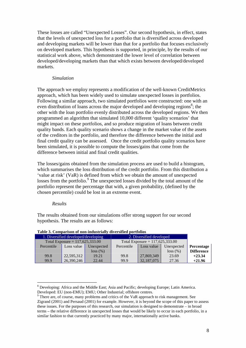
Table 3. Comparison of non-industrially diversified portfolios1. Diversified developed/developing 2. Diversified developed

Total Exposure = 117,625,333.00 Total Exposure = 117,625,333.00Percentile Loss value Unexpected

loss (%)Percentile Loss value Unexpected

loss (%)PercentageDifference

99.8 22,595,312 19.21 99.8 27,869,349 23.69 +23.3499.9 26,390,246 22.44 99.9 32,187,075 27.36 +21.96

8 Developing: Africa and the Middle East; Asia and Pacific; developing Europe; Latin America.Developed: EU (non-EMU); EMU; Other Industrial; offshore centres.9 There are, of course, many problems and critics of the VaR approach to risk management. SeeZigrand (2001) and Persaud (2001) for example. However, it is beyond the scope of this paper to assessthese issues. For the purposes of this research, our simulation is designed to demonstrate – in broadterms – the relative difference in unexpected losses that would be likely to occur in each portfolio, in asimilar fashion to that currently practiced by many major, internationally active banks.

9

As can be seen from table 3, the unexpected losses simulated for the portfolio focusedon developed country borrowers are, on average, almost twenty-three percent higherthan for the portfolio diversified across developed and developing countries.

DiscussionThe simulated loan portfolios constructed offer clear evidence that the benefits ofinternational diversification produce a more efficient risk/return trade-off for banks atthe portfolio level. Given that capital requirements are intended to deal withunexpected loss, the fact that the level of unexpected loss in our simulation is lowerfor a diversified than for an undiversified portfolio, suggests that – in order toaccurately reflect the actual risks that banks may face – Basel II should take accountof this effect.

It is, of course, always possible to question the assumptions which underpin anysimulation. We have attempted to ensure that our assumptions are as reasonable aspossible. One aspect that we considered in detail was that the decision to assume noindustrial diversification within countries might prevent the benefits of suchdiversification in developed countries – which generally have a greater range ofindustries than do developing countries – from being taken into account. Weconcluded, however, that the potential benefits of such diversification may havetraditionally been overstated. This position is supported by recent empirical workundertaken by the BIS.10 Using data from 105 Italian banks, over the period 1993-1999, Acharya et al (2002) test empirically for evidence in support of the theoreticalbenefits of industrial, sectoral and geographical diversification. The results, thoughsomewhat surprising, would seem to offer support for both the assumptions thatunderpin the loan portfolio simulation (i.e. no industrial diversification) and, crucially,the general findings or our empirical work.

From the combined results on bank loan return and risk, we conclude that increased industrial loandiversification results in an inefficient risk-return trade-off for the (Italian) banks in our sample, and

sectoral diversification results in an inefficient risk-return trade-off for banks with relatively highlevels of risk. Geographical diversification on the other hand does result in an improvement in the risk-

return trade-off for banks with low or moderate levels of risk. (op. cit: 5)

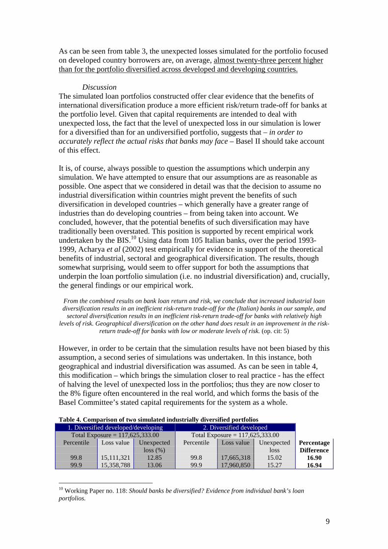
However, in order to be certain that the simulation results have not been biased by thisassumption, a second series of simulations was undertaken. In this instance, bothgeographical and industrial diversification was assumed. As can be seen in table 4,this modification – which brings the simulation closer to real practice - has the effectof halving the level of unexpected loss in the portfolios; thus they are now closer tothe 8% figure often encountered in the real world, and which forms the basis of theBasel Committee’s stated capital requirements for the system as a whole.

Table 4. Comparison of two simulated industrially diversified portfolios1. Diversified developed/developing 2. Diversified developed

Total Exposure = 117,625,333.00 Total Exposure = 117,625,333.00Percentile Loss value Unexpected

loss (%)Percentile Loss value Unexpected

lossPercentageDifference

99.8 15,111,321 12.85 99.8 17,665,318 15.02 16.9099.9 15,358,788 13.06 99.9 17,960,850 15.27 16.94

10 Working Paper no. 118: Should banks be diversified? Evidence from individual bank’s loanportfolios.

10

The difference between the simulated unexpected losses in the two portfolios has alsobeen reduced by this modification, although less so. However, at almost seventeenpercent, on average, the difference remains highly significant, and so offers furtherevidence of the robustness of our results.

Another issue that we have given consideration to is the fact that correlations are notconstant over time. The danger, of course, is that correlations within emergingmarkets increase dramatically in crises, as contagion spreads the crisis from onecountry or region to another. In this instance, it is possible that a portfolio diversifiedacross a range of emerging and developing regions, might be hit simultaneously ineach of these areas. However, while this may well be the common perception ofemerging market behaviour in crises, it may only apply to a limited number of cases,which require specific preconditions to be in place; preconditions, which at thecurrent time – and indeed at most times - do not apply. Kaminsky, Reinhart and Vegh(2002) examine two hundred years of financial crises, in both developed anddeveloping countries, for evidence of contagion. They conclude that ‘fast and furious’contagion of the type described above, and often viewed as inherent in emergingmarkets may occur, but only under certain circumstances. Of the major emergingmarket crises since 1980, the Mexican default of 1982, the Mexican devaluation of1994, the devaluation of the Thai baht in 1997 and the Russian default of 1998, wereall seen as instances where significant contagion did occur. However, with theexception of the Russian default – which affected all emerging and developingregions, as well as the developed world to a surprising extent (Davis, 1999) - theresultant contagion was restricted to the same region. Consequently, a portfoliodiversified across all emerging and developing regions would not have sufferedsimultaneous problems to the extent described above. On the other hand, more recentevents, such as the Brazilian devaluation of 1999, Turkey’s devaluation in early 2001and the problems starting in Argentina towards the end of 2001, have been associatedwith far less contagion, and have not become an emerging market-wide phenomenon.

Kaminsky et al (op. cit) suggest that a crisis that spreads beyond regional boundariesrequires an investment boom, or bubble, to precede it. In this way, actors beyond theregion become involved in events there, and so the crisis may spread – via commoncreditors to some extent – to other emerging, and even developing regions. Thecurrent environment is certainly not one of boom with regard to capital flows toemerging and developing economies. Furthermore, it seems unlikely that suchcircumstances are likely to reoccur in the foreseeable future, ensuring that thepreconditions required for system-wide contagion are not in place, and the benefits ofwidespread diversification will remain a reality.

Kaminsky and Reinhart (2002) also emphasise this point. Their research suggests thatfinancial turmoil in the ‘periphery’ (developing countries) only has systemicimplications, such as contagion beyond the immediate region, when asset markets inone of the financial centres (developed world) is affected. “Thus, financial centersserve a key role in propagating financial turmoil. When financial centers remain safe,problems in an emerging market stop at the region’s border”. (p.3)

11

IV. Conclusion

The expressed purpose of the proposed new Basel Capital Accord is to better alignregulatory capital with actual risk. This process, it is argued, will put bank lending ona sounder regulatory footing and remove the many distortions that have come to berecognised in the existing accord. We have argued that the current proposals run therisk of causing an increase in cost and/or reduction in quantity of bank lending todeveloping countries, as a consequence of the sharp increase in capital requirementsfor lending to lower rated borrowers. The response to this argument is that anychanges in capital requirements are justified on the basis that, whilst the capitalassociated with lower (higher) rated borrowers is to rise (fall) significantly, relative tothe existing situation, this merely reflects the more accurate measurement of risk.

However, as we have demonstrated in this paper, the failure of the proposals to date totake account of the benefits of international diversification suggests that, in thisinstance at least, risk is not been accurately measured. That is, by excluding thepossibility that banks’ capital requirements should take account of portfolio anddiversification effects, the proposals effectively impose an inaccurate measure ofactual risk, at the portfolio level. At present, the most sophisticated banks often dotake account of the benefits of diversification in their international lending decisions.The fact that the proposals under Basel II will not allow these diversification benefitsto be taken into account, suggests that the regulatory capital associated with lending todeveloping countries will be higher than that which the banks would – and currentlyare – choosing to put aside on the basis of their own models.

The Basel Committee has already made a number of modifications to the originalproposals of January 2001 (CP2). The most significant being the modifications to theIRB formula to take account of variable asset correlation as related to PD, and thoserelating to SMEs. Following the release of CP2 there was widespread concern thatlending to SMEs would be adversely affected by a large increase in the capitalrequirements associated with such lending. After intensive lobbying the BaselCommittee has reconsidered the issue. The general changes to the IRB formula withrespect to corporate lending – wherein the curve has been significantly flattened – willobviously be of benefit to SMEs. However, the Basel Committee has gone further.July 2002 saw the release of a document by the Basel Committee, which highlightedmajor areas where agreement had been reached. Of these, it was agreed that thetreatment of SMEs should be as follows:

In recognition of the different risks associated with SME borrowers, under the IRB approach forcorporate credits, banks will be permitted to separately distinguish loans to SME borrowers (definedas those with less than Euro 50 mn in annual sales) from those to larger firms. Under the proposedtreatment, exposures to SMEs will be able to receive a lower capital requirement than exposures to

larger firms. The reduction in the required amount of capital will be as high as twenty percent,depending on the size of the borrower, and should result in an average reduction of approximately ten

percent across the entire set of SME borrowers in the IRB framework for corporate loans.11

Thus, in the case of SME and corporate lending, the Basel Committee has recognisedthe impact that differential asset correlation can have on portfolio level risk. Our

11 Basel Committee reaches agreement on New Capital Accord issues.http://www.bis.org/press/p020710.htm

12

results strongly suggest that a similar modification is justified with respect tointernationally diversified lending.

The specific manner that the Basel Committee might want to incorporate thesefindings is, of course, best left to them. Given the experience and expertise at theirdisposal we would not at this stage want to offer suggestions as to the means by whichthese modifications might be made. However, given the changes already made to theIRB formula with respect to corporates and SMEs, as well as the fact that the changeswe propose would seem to have at least as solid an empirical basis, there are notheoretical, empirical or practical reasons why changes should not be made toincorporate the benefits of international diversification. We therefore urge the BaselCommittee to incorporate these findings in the final consultative paper, due forrelease in Spring 2003, and would be happy to collaborate with the Committee in thisimportant work, if it was considered useful.

References:Acharya, V., Hasan I, and Saunders A (2002) Should banks be diversified? Evidencefrom individual bank loan portfolios. BIS Working Paper no. 118.

Davis, E.P. (1999) Russia/LTCM and market liquidity risk", The Financial Regulator,4/2, Summer.

Griffith-Jones, S. (2002) Capital Flows to Developing Countries: Does the EmperorHave Clothes? Mimeo, Institute of Development Studies

Griffith-Jones, S. and Spratt, S. (2001) 'Will the proposed new Basel Capital Accordhave a net negative effect on developing countries?' mimeo, Institute of DevelopmentStudies, Brighton

Griffith-Jones, S., Spratt S. and Segoviano, M. (2002) Basel II and DevelopingCountries, The Financial Regulator, vol. 7, No. 2, September.

J.P. Morgan, (1997), “Creditmetrics Technical Document”

Kaminsky, Reinhart and Vegh (2002) Two Hundred Years of Contagion.Forthcoming.

Kaminsky and Reinhart (2002) The Center and the Periphery: The Globalization ofFinancial Turmoil. Forthcoming.

Markowitz, Harry, (1959), “Portfolio Selection: Efficient Diversification ofInvestments”, John Wiley and Sons.

Merton, Robert C., (1974), “On the pricing of corporate debt: The risk structure ofinterest rates”, The Journal of finance, Vol 29, pp449-470

Persaud (2001) Sending the Herd off the Cliff-Edge: The Disturbing InteractionBetween Herding and Market-Sensitive Risk Management Practices. Winner of the

13

Institute of International Finance’s Jacques de Larosiere essay on global finance,2000.

Segoviano, M. (1998) Basel II v.s. Creditmetrics, LSE, Msc Economics disseration.

Zigrand, J.P. and Danielsson, J (2001) “What happens when you regulate risk?Evidence from a simple equilibrium model”, FMG/LSE, DP393

14

Annex 1. Cumulative Distribution Function Tests (C.D.F)

Figure 1. C.D.F Test for Correlations on Syndicated Loan Spreads (1993-2002)

00.20.40.60.8

11.2

Deved/DevingDeved/Deved

Figure 2. C.D.F.Test for Correlations on Banks' Return on Capital (1988-2001)

00.20.40.60.8

11.2

Deved/DevingDeved/Deved

Figure 6. C.D.F. Tests for Correlations on Stock Exchange Movements (IFC I-COMP: 1990-2002)

00.20.40.60.8

11.2

Deved/DevingDeved/Deved

Figure 7. C.D.F. Tests for Correlations on Stock Exchange Movements (IFC G-COMP: 1990-2002)

00.20.40.60.8

11.2

Deved/DevingDeved/Deved

Figure 8. C.D.F Tests for Correlations on Bond Market Movements

(GBI-EMBI+: 1991-2002)

00.20.40.60.8

11.2

Series1Series2

Figure 3. C.D.F Test for Correlations on Banks' Return on Assets (1988-2001)

00.20.40.60.8

11.2

Deved/DevingDeved/Deved

Figure 4. C.D.F Test for Correlations on GDP Growth (1985-2000)

00.20.40.60.8

11.2

Deved/DevingDeved/Deved

Figure 5. C.D.F Test for Correlations on Real Short-Term Interest Rates (1985-2000)

00.20.40.60.8

11.2

Deved/DevingDeved/Deved

15

Appendix: Computation of Unexpected Losses

Considering that the quality of the credit portfolio of any bank can change at any timein the future, there is a need to make frequent calculations of the expected losses thata bank could suffer under different risk situations. Given the constant changes inportfolio quality, it is unlikely that the computed expected losses will be the same fordifferent periods. The difference between expected losses computed at differentperiods, (due to changing credit quality), is the cause of potential losses to the bank,that could erode their capital in extreme situations. These losses are called“Unexpected Losses” and their estimation represents the issue to be addressed in thisappendix.

Unexpected Losses arise because of joint credit quality changes among the credits thatconform a credit portfolio. In order to model such joint credit quality changes, weadopted a portfolio approach.

The adoption of the portfolio approach (See Markowitz (1959)) has been amplydocumented and adopted in diverse finance applications. Under this theory, investorsformulate their investment portfolio, taking care of the optimal risk-return relationshipthat a given portfolio has. With this in mind, credit risk modellers have alreadydeveloped risk management techniques aimed to take account of the portfoliodiversification effect. Although such approaches might be subject to improvements12,we do believe that portfolio diversification could and should be an integral part ofcredit risk valuation for regulation purposes. As we have argued in the main body ofpaper and in previous work, we believe that negative economic outcomes will beprovoked by the fact that the proposed regulation framework only punishes high-risktaking but does not provide incentives for portfolio diversification.

In this appendix we present a modification to the “Credit-Metrics”13 methodology thathas been used to simulate credit unexpected losses of analysed portfolios. The Credit-Metrics model has been described as: “A full portfolio view addressing credit eventcorrelations which identify the costs of over concentration and benefits ofdiversification”. (See J.P. Morgan (1997)). The objective of this appendix is to presentthe modifications that were made to the Credit-Metrics approach in order to makepossible its implementation. For detailed exposition refer to the Credit-Metricstechnical document. We refer to the modification to the “Credit-Metrics”methodology as Full Credit Risk model: FCRM.

Full Credit Risk Model:Empirical studies that show that credit defaults are correlated have been widelypresented, here we present evidence that credit risk can also be diversified.In order to calculate portfolio diversification, it would be necessary to know theprobability that each of the credits making up a portfolio migrate jointly from theircurrent rating (credit quality) to each of the possible ratings. For this, we would 12 It is not our intention at this point to analyse the possible improvements to each methodology.13 The choice of this model was made in terms of simplicity for modelling and availability of data. It isnot our intention to favour any specific credit risk modelling technique.

16

require to know a number of tables of joint probabilities equivalent to the number ofpairs of credits making up a portfolio. This objective is unattainable given the lack ofreliable data, the amount and complexity of it.

The CreditMetrics’ approach makes use of two main elements:

I. The Merton Approach to model Credit Quality Changes.II. An indirect approach to model Correlations among the credits that make up a creditportfolio.

Finally, once a correlations matrix among the creditors making up the credit portfoliois built, this methodology simulates the unexpected losses for the portfolio.

I. The Merton Approach to model Credit Quality Changes.The Merton approach assumes that equity can be viewed as a call option on the firms’assets with a strike price equal to the book value of the firm’s debts (See Merton(1974)). The intuition behind this assumption is that given the limited liability featureof equity, equity holders have the right but not the obligation to payoff debt-holdersand take over the remaining assets of the firm. This approach implies that the creditquality (rating) of a given creditor is related to the difference between the marketvalue of its assets and its debt.

Under this approach, the change in the value of the assets of a given company isrelated to the change in its rating. Therefore, the distribution of the company’s assetsreturns can be used to calculate the distribution of its rating change's probabilities.For the generalisation of this model, it is necessary to include, in addition to thedefault state, different credit quality states.

Figure A.1: The Distribution of Assets’ Returns.

AE CD B

Z e Z d Z c Z b

The transition matrix is the variable that summarises the migration probabilities fromone credit quality to any other. Having the transition probabilities between differentcredit qualities and considering the Merton Approach, it is possible to derive themarket value of assets that represent the cut-off values between different creditqualities, as shown in Figure 1. These cut-off values fulfil the condition that if thechange in the market value of the asset (r) is sufficiently negative, (i.e. smaller thanZE ), then the credit falls into default; if ZE < r < ZD, the credit is rated D, and so on.

17

Taking into consideration the empirical transition matrix, it is possible to estimate theprobability of these changes happening as follows: (for a credit initially rated as X).

Prob(E|X) = Prob(r < ZE) = ϕ(ZE)Prob(D|X) = Prob(ZE <r < ZD) = ϕ(ZD) - ϕ(ZE)Prob(C|X) = Prob(ZD <r < ZC) = ϕ( ZC) - ϕ(ZD)Prob(B|X) = Prob(ZC <r < ZB) = ϕ(ZB) - ϕ(ZC)Prob(A|X) = Prob(ZB <r < ZA) = 1 - ϕ(ZB)

Where:R: Is the implied market value of assets.ϕ: Is the cdf for the Normal distributionFrom this point of view, the correlation matrix of changes of credit quality betweencreditors can be computed by developing an explanatory model of the changes in thevalue of the assets of the debtors.

This approach presents several practical problems for implementation, the mostimportant being the handling of very large correlation matrices. Additionally, it is notpossible to obtain the changes in the market value of assets for each particular debtor,since it would be necessary to have specific information about the internal financialstructure of each debtor. These two disadvantages make it impossible to implement anideal correlation matrix, for these reasons we will adopt an indirect ( but moremanageable) method to introduce the portfolio diversification effect.

II. An indirect approach to model Correlations among the credits that make upa credit portfolio.Following the Merton’s approach, J.P. Morgan makes an a-priori distinction of thefactors that determine the changes in the value of the assets of the debtors. Thisdistinction comes from two basic components: the market component and theidiosyncratic component. By definition, the idiosyncratic component does notcorrelate with anything, since it refers to those factors unique for the debtor. But themarket component has with it, all the elements that allow the portfolio diversification.rtotal = WM rmarket + WI rIdiosyncratic 1)Where:WM: Percentage of returns explained by the market component14.rmarket: Market component of returns.WI : Percentage of returns explained by the idiosyncratic component15.Iidiosyncratic: Idiosyncratic component of returns.

14 In the CreditMetrics technical document, it is explained how these weights can be calculated. Afterempirical implementations, it is proved that an acceptable value of WM = 70%. For our exercise, weassume this value.

15 The idiosyncratic component weight is obtained with the following equation:

w wI M= −1 2

The objective of this equation is to be consistent with the change in the market value of the assets’standardized returns.

18

Conversely, the market component of Returns is defined as:rMarket = HA rGDP Country + (1-HA) rGDP Economic Activity 2)Where:HA: Percentage of market component explained by the GDP of the debtor’s country.The Herfindahl Index computes this parameter.rGDP Country: Return on the GDP of the debtor’s country.(1-HA): Percentage of market component explained by the GDP of the debtor’scountry.rGDP Economic Activity: Return on the GDP of the debtor’s Economic Activity.

The market component of returns is divided between economic activity andgeographical area. Which is more relevant for a debtor? Is it his economic activity orthe country where his business takes place? The percentage of participation of thesemarket factors in the debtor’s systemic risk is exogenous to the model. Therefore amethodology was designed to solve this problem in the most objective way possible(See Segoviano (1998)).

This methodology was based in the fact that the greater the variety of economicactivities in a country, the lesser the effect (on the value of assets of a debtor in thatcountry) of a sudden change in the country’s production. Within this framework it ispossible to infer that in those countries in which there are a few economic activities(and therefore there is a high economic activity concentration), the most importantfactor for the debtor’s assets value will be his geographic location. The intuitionbehind this reasoning is the fact that if the country is affected by an economic shock,it is very likely that debtor will experience a decrease in the value of his assets, sinceit is highly probable that the debtor will belong to the economic activities that havebeen affected.

Following this reasoning, we computed a “Herfindahl” index with the followingformula for each group of countries:

HX

XA

Ai

Ajj

ni

n

=

=

=∑

∑

1

1

2

(3)

Where:XAi = is the amount of participation of the i economic activity in country group A.16

Once considered all the elements that compose the market component of assets’returns the next step is to calculate the correlations between the debtors making up acredit portfolio. Given a pair of debtors X and Y, working in B and V industrial activities; located inA and E country groups and with returns expressed in the following way:

16 The higher the Herfindhal index for a given country group, the less economic activity diversified.Then, the percentage of the market component explained by the GDP of the debtor’s country takesmore importance.

19

r w r w H r w H rX IX IX MX A A MX A B= + + −( )1

r w r w H r w H rY IY IY MY E E MY E V= + + −( )1

The problem of estimating the correlations among each couple of creditors in theportfolio is summarised in the following way:

ρ ρ ρXY MX A MY E AE MX A MY E BVw H w H w H w H= + − −( ) ( )1 1 17 (4)

Where:pAE: is the correlation between different country groups18.pBV: is the correlation between different economic activities19.

This equation is computed for each pair of debtors making up the portfolio. Theresults of computing this equation are compiled in a (n x n) square matrix, where n isthe number of creditors in the portfolio. This matrix is named the correlation matrixbetween creditors and is unique for each portfolio. This matrix is an extremelyimportant variable for the simulation of unexpected losses, since it incorporates thenecessary elements to quantify the concentration/diversification of the portfolio.

With these elements, we show in the following section how quality scenarios for theportfolio are simulated. From these quality scenarios, the loss distribution is builtfrom which it is possible to obtain the unexpected losses.

III Simulation of quality scenarios for the credit portfolioCombining the transition matrix with the correlation matrix between creditors, wesimulate quality scenarios from which the loss distribution for the credit portfolio isobtained.As explained above, the transition matrix indicates the probabilities of quality changesthat a creditor with a given rating might experience. Additionally, the correlations ofquality changes between creditors is involved. Creditors with similar characteristicswill tend to migrate jointly to different credit qualities when hit by economic shocks.Creditors with different characteristics will tend to migrate dis-jointly to differentcredit qualities when hit by economic shocks. This implies that credit portfoliosconcentrated in credits with similar characteristics will tend to have higherunexpected losses since they will not be diversifying the possible economic risks.

We programmed an algorithm to compute 10,000 possible quality scenarios for eachof the (n x n) couples of creditors that make up the portfolio. Each quality scenario 17 Since the correlations between idiosyncratic components and geographical components,idiosyncratic components and economic activity components as well as between economic activitiesand geographical components are assumed to be zero.18 These correlations were computed between the spreads of syndicated loans for each country group.We considered that such spreads represent the riskiness of the financial system in each country group.19 These correlations were computed between indexes for each of the economic activities considered inthe excercise. Each economic activity index was built with the economic activity component of theGDP of a representative country for each country group in the sample.

20

shows a change in the market value of the assets of the creditors in the portfolio. Thisprocess is repeated 10,000 times. The quality changes of the members of the portfolioallow generating an amount of losses or profits that conform the loss distribution ofthe portfolio.

In order to generate these scenarios, the following process is computed:

1. Generation of random uniform numbers.2. Transformation of this random numbers into normal standard random numbers.3. Transformation of the normal standard random numbers into normal multivariated

random numbers with variance equal to the correlation matrix between creditors.

Since it was assumed that the process that generates changes in the assets follows anormal distribution, we use normal random multivariated distribution to generate jointquality migrations, where credits with high correlation will tend to migrate jointly.

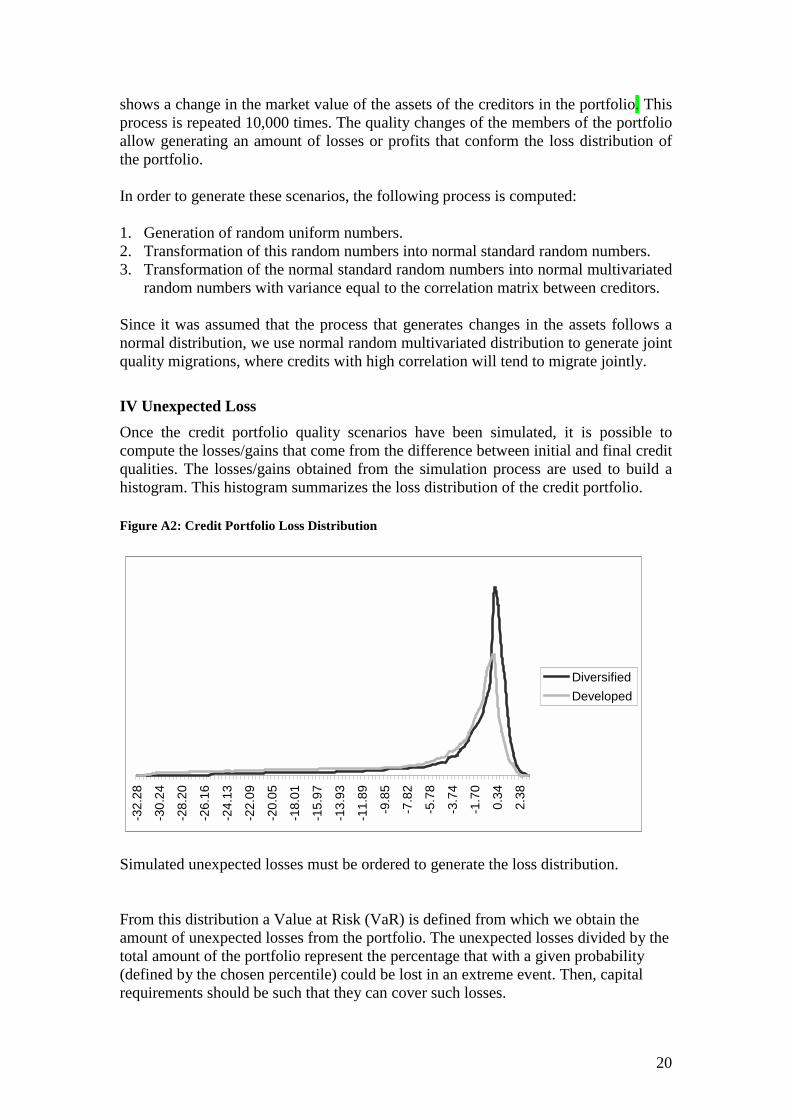
IV Unexpected LossOnce the credit portfolio quality scenarios have been simulated, it is possible tocompute the losses/gains that come from the difference between initial and final creditqualities. The losses/gains obtained from the simulation process are used to build ahistogram. This histogram summarizes the loss distribution of the credit portfolio.

Figure A2: Credit Portfolio Loss Distribution

-32.

28

-30.

24

-28.

20

-26.

16

-24.

13

-22.

09

-20.

05

-18.

01

-15.

97

-13.

93

-11.

89

-9.8

5

-7.8

2

-5.7

8

-3.7

4

-1.7

0

0.34

2.38

DiversifiedDeveloped

Simulated unexpected losses must be ordered to generate the loss distribution.

From this distribution a Value at Risk (VaR) is defined from which we obtain theamount of unexpected losses from the portfolio. The unexpected losses divided by thetotal amount of the portfolio represent the percentage that with a given probability(defined by the chosen percentile) could be lost in an extreme event. Then, capitalrequirements should be such that they can cover such losses.

21

.