basic category theory (oplss 2016)
TRANSCRIPT
Basic Category Theory(OPLSS 2016)
Edward MorehouseCarnegie Mellon University
June 2016(revised June 30, 2016)

Contents
1 Basic Categories 31.1 Definition of a Category . . . . . . . . . . . . . . . . . . . . . . . 31.2 Diagrams . . . . . . . . . . . . . . . . . . . . . . . . . . . . . . . 51.3 Structured Sets as Categories . . . . . . . . . . . . . . . . . . . . 6
1.3.1 Discrete Categories . . . . . . . . . . . . . . . . . . . . . . 61.3.2 Preorder Categories . . . . . . . . . . . . . . . . . . . . . 71.3.3 Monoid Categories . . . . . . . . . . . . . . . . . . . . . . 7
1.4 Categories of Structured Sets . . . . . . . . . . . . . . . . . . . . 81.4.1 The Category of Sets . . . . . . . . . . . . . . . . . . . . . 81.4.2 The Category of Preorders . . . . . . . . . . . . . . . . . 91.4.3 The Category of Monoids . . . . . . . . . . . . . . . . . . 9
1.5 Categories of Types and Terms . . . . . . . . . . . . . . . . . . . 91.6 Categories of Categories . . . . . . . . . . . . . . . . . . . . . . . 11
1.6.1 Functors . . . . . . . . . . . . . . . . . . . . . . . . . . . . 111.6.2 The Special Role of Sets . . . . . . . . . . . . . . . . . . . 13
1.7 New Categories from Old . . . . . . . . . . . . . . . . . . . . . . 151.7.1 Ordered Pair Categories . . . . . . . . . . . . . . . . . . . 151.7.2 Subcategories . . . . . . . . . . . . . . . . . . . . . . . . . 171.7.3 Opposite Categories . . . . . . . . . . . . . . . . . . . . . 181.7.4 Arrow Categories . . . . . . . . . . . . . . . . . . . . . . . 191.7.5 Slice Categories . . . . . . . . . . . . . . . . . . . . . . . . 21
2 Behavioral Reasoning 232.1 Monic and Epic Morphisms . . . . . . . . . . . . . . . . . . . . . 23
2.1.1 Monomorphisms . . . . . . . . . . . . . . . . . . . . . . . 232.1.2 Epimorphisms . . . . . . . . . . . . . . . . . . . . . . . . 25
2.2 Split Monic and Epic Morphisms . . . . . . . . . . . . . . . . . . 262.3 Isomorphisms . . . . . . . . . . . . . . . . . . . . . . . . . . . . . 28
3 Universal Constructions 313.1 Terminal and Initial Objects . . . . . . . . . . . . . . . . . . . . . 31
3.1.1 Terminal Objects . . . . . . . . . . . . . . . . . . . . . . . 313.1.2 Unit Type . . . . . . . . . . . . . . . . . . . . . . . . . . . 333.1.3 Global and Generalized Elements . . . . . . . . . . . . . . 33
i
ii CONTENTS
3.1.4 Initial Objects . . . . . . . . . . . . . . . . . . . . . . . . 343.1.5 Void Type . . . . . . . . . . . . . . . . . . . . . . . . . . . 35
3.2 Products . . . . . . . . . . . . . . . . . . . . . . . . . . . . . . . . 353.2.1 Products of Objects . . . . . . . . . . . . . . . . . . . . . 353.2.2 Product Functors . . . . . . . . . . . . . . . . . . . . . . . 393.2.3 Product Types . . . . . . . . . . . . . . . . . . . . . . . . 413.2.4 Finite Products . . . . . . . . . . . . . . . . . . . . . . . . 423.2.5 Typing Contexts . . . . . . . . . . . . . . . . . . . . . . . 45
3.3 Coproducts . . . . . . . . . . . . . . . . . . . . . . . . . . . . . . 473.3.1 Coproducts of Objects . . . . . . . . . . . . . . . . . . . . 473.3.2 Coproduct Functors . . . . . . . . . . . . . . . . . . . . . 493.3.3 Sum Types . . . . . . . . . . . . . . . . . . . . . . . . . . 503.3.4 Distributive Categories . . . . . . . . . . . . . . . . . . . . 50
3.4 Exponentials . . . . . . . . . . . . . . . . . . . . . . . . . . . . . 533.4.1 Exponentials of Objects . . . . . . . . . . . . . . . . . . . 533.4.2 Exponential Functors . . . . . . . . . . . . . . . . . . . . 573.4.3 Function Types . . . . . . . . . . . . . . . . . . . . . . . . 59
3.5 Cartesian Closed Categories . . . . . . . . . . . . . . . . . . . . . 59
4 Two Dimensional Structure 614.1 Naturality . . . . . . . . . . . . . . . . . . . . . . . . . . . . . . . 61
4.1.1 Natural Transformations . . . . . . . . . . . . . . . . . . . 614.1.2 Functor Categories . . . . . . . . . . . . . . . . . . . . . . 62
4.2 2-Categories . . . . . . . . . . . . . . . . . . . . . . . . . . . . . . 634.2.1 2-Dimensional Categorical Structure . . . . . . . . . . . . 634.2.2 String Diagrams . . . . . . . . . . . . . . . . . . . . . . . 68
4.3 Adjunctions . . . . . . . . . . . . . . . . . . . . . . . . . . . . . . 704.3.1 Behavioral Characterization . . . . . . . . . . . . . . . . . 704.3.2 Structural Characterizations . . . . . . . . . . . . . . . . 714.3.3 Conversion Relations . . . . . . . . . . . . . . . . . . . . . 754.3.4 Context Distributivity Revisited . . . . . . . . . . . . . . 76

Introduction
Category theory can be thought of as a sort of generalized set theory, where theprimitive concepts are those of set and function, rather than set and member-ship. This shift of perspective allows categories to more directly describe manystructures, even those that are not particularly set-like. In category theory, theprimitive concept of set generalizes to that of object, and function to morphism.
The only assumption that we make about these generalized functions is thatthey support a composition structure, whereby any configuration of compatiblemorphisms can be combined to yield a new morphism, and the details of how wego about combining the parts into a whole doesn’t matter, only the configurationof those parts does.
This is reminiscent of many aspects of our physical world. When we builda castle out of Lego bricks, the order in which we assembled the bricks is notrecorded anywhere in the finished product, only their configuration with respectto one another remains.
By beginning from very few assumptions, category theory permits a great dealof axiomatic freedom. Additional postulates (e.g. the axiom of choice) can thenbe selectively reintroduced in order to characterize a particular object theory ofinterest (e.g. set theory).
Because categorical characterizations are based on the concepts of object andmorphism, they must describe their subjects behaviorally (or externally), ratherthan structurally (or internally): in category theory we can’t pin down whatthe objects of our study actually are, only how they relate to one another viamorphisms. In this sense, category theory is the sociology of formal systems.
For example, we will see how we can characterize the cartesian product once andfor all using a universal property. This allows us to describe cartesian products ofsets, of groups, of topological spaces, of types, of propositions, and of countlessother things, all in one fell swoop, rather than on a tedious case-by-case basis.
1

2 CONTENTS

Chapter 1
Basic Categories
1.1 Definition of a Category
Definition 1.1.0.1 (category) A category ℂ consists of the following data:
• A collection of objects, ℂ0 (comprising the 0-dimensional part of ℂ).We write “A ∶ ℂ” to indicate that A ∈ ℂ0.
• A collection of morphisms or “arrows”, ℂ1 (the 1-dimensional part).We write “𝑓 ∶∶ ℂ” to indicate that 𝑓 ∈ ℂ1.
• Two morphism boundary maps from arrows to objects:domain, “∂−”, and codomain, “∂+”.For ℂ-objects A and B, we indicate the collection of ℂ-arrows with domainA and codomain B by “ℂ (A → B)”, and call this collection “hom”1. Whenthe category in question is obvious or irrelevant, we just write “A → B”.We indicate that an arrow 𝑓 is a member of this collection by writing“𝑓 ∶ ℂ (A → B)” or “𝑓 ∶ A → B”.
• An identity morphism map from objects to arrows, “id”, such that bothboundaries of an object’s identity arrow are just that object itself:
id(A) ∶ A → A
• A partial binary function on arrows, morphism composition, “– ⋅ –”,that is defined just in case the codomain of the first is equal to the domainof the second, in which case the composite arrow has the domain of thefirst and codomain of the second:
if 𝑓 ∶ A → B and 𝑔 ∶ B → C then 𝑓 ⋅ 𝑔 ∶ A → C1presumably, short for “homomorphisms”
3

4 CHAPTER 1. BASIC CATEGORIES
This data is required to respect the following relations.
• composition left unit law: for an arrow 𝑓 ∶ A → B,
id(A) ⋅ 𝑓 = 𝑓
• composition right unit law: for an arrow 𝑓 ∶ A → B,
𝑓 ⋅ id(B) = 𝑓
• composition associative law: for arrows 𝑓 ∶ A → B, 𝑔 ∶ B → C andℎ ∶ C → D,
(𝑓 ⋅ 𝑔) ⋅ ℎ = 𝑓 ⋅ (𝑔 ⋅ ℎ)
By the associative law we may unambiguously write compositions without usingbrackets.Definition 1.1.0.2 In order to avoid gratuitously naming the boundaries ofarrows, we will call a pair of arrows 𝑓 , 𝑔 ∶∶ ℂ:
• coinitial, or a “span”, if ∂−(𝑓) = ∂−(𝑔),• coterminal, or a “cospan”, if ∂+(𝑓) = ∂+(𝑔),• composable if ∂+(𝑓) = ∂−(𝑔),• parallel if both coinitial and coterminal, and
• anti-parallel if composable in both orders.
Additionally, we will call an arrow an endomorphism if it is composable withitself, and a list of arrows a path if they are serially composable, that is, if∂+(𝑓𝑖) = ∂−(𝑓𝑖+1) for the list [𝑓0 , ⋯ , 𝑓𝑛].Remark 1.1.0.3 (applicative order composition) It is common to see the com-position 𝑓 ⋅ 𝑔 written as “𝑔 ∘ 𝑓”. This can be useful when we want to apply acomposite morphism to an argument in a category where a morphism is somesort of function. Then (𝑔 ∘ 𝑓)(𝑥) = 𝑔(𝑓(𝑥)), which coincides with our custom towrite function application with the argument on the right. It may help to read“𝑓 ⋅ 𝑔” as “𝑓 then 𝑔”, and to read “𝑔 ∘ 𝑓” as “𝑔 after 𝑓”.Remark 1.1.0.4 (dimensional promotion) It is often convenient to call theidentity arrow on an object by the same name as the object itself, e.g. to write“A” in place of id(A). This is called dimensional promotion, and will becomeuseful as we introduce more complex arrow constructions and concision becomesmore of an issue.Remark 1.1.0.5 (unbiased presentation) There is an equivalent presentation ofcategories in terms of unbiased composition. There, instead of a single binarycomposition operation acting on a composable pair of arrows, we have a length-indexed composition operation for paths of arrows (still with unit and associativelaws). In this presentation, an identity morphism is a nullary composition, a

1.2. DIAGRAMS 5
morphism itself is a unary composition, and in general, any length 𝑛 path ofarrows has a unique composite. Although more cumbersome to axiomatize, anunbiased presentation of categories makes it easier to appreciate the idea at theheart of the definition: every composable configuration of things should have aunique composite.Exercise 1.1.0.6 (uniqueness of composition units) By definition, identity ar-rows act as (two-sided) units for composition. Prove that they are the onlyarrows with this property.
Hint (proof by Fight Club): suppose there were another arrow, id′ ∶ A → A,that acted as a unit for composition at A, then what would we know about thecomposite id(A) ⋅ id′(A)?
1.2 Diagrams
We think of an arrow as emanating from its domain and proceeding to itscodomain. We can represent configurations of arrows of a category using adirected graph whose vertices are labeled by objects of the category and whoseedges are labeled by arrows. Such a graph is known as a diagram, for example:
A B C𝑓 𝑔
We can represent equations between arrows using diagrams as well. We say thata diagram is commuting or “commutes” if the composites of parallel pathsdepicted in the diagram are equal. For example, the fact that each pair ofcomposable arrows has a unique composite gives us commuting compositiontriangles, such as:
B
A C
𝑓 𝑔
𝑓 ⋅ 𝑔
Commuting diagrams may be extended by pre- or post-composition of arrows.This is called whiskering, and depicts the fact that equality of morphisms isa congruence with respect to composition: if 𝑔1 = 𝑔2 then 𝑓 ⋅ 𝑔1 = 𝑓 ⋅ 𝑔2 and𝑔1 ⋅ ℎ = 𝑔2 ⋅ ℎ whenever the composites are defined. The name comes from thefact that the arrows pre- or post-composed to the diagram look like whiskers:
A B C D𝑓𝑔1
𝑔2
ℎ

6 CHAPTER 1. BASIC CATEGORIES
Pairs of commuting diagrams may also be combined along a common path. Thisis called pasting, and depicts the transitivity of equality: if 𝑓1 = 𝑓2 and 𝑓2 = 𝑓3then 𝑓1 = 𝑓3.
We may express the unit and associative laws for composition succinctly usingcommuting diagrams:
A
A B
B
id
id
𝑓
𝑓
𝑓 and
A C
B D𝑓
𝑔 ℎ
𝑓 ⋅ 𝑔
𝑔 ⋅ ℎ
In the diagram for unitality (left), the triangles representing the left and rightunit laws are pasted together along the singleton path [𝑓]. In the diagram forassociativity (right), each of the two composition triangles is whiskered by anarrow (ℎ and 𝑓 , respectively), and the resulting diagrams are pasted togetheralong the shared path [𝑓 , 𝑔 , ℎ].In the graphical language of diagrams, any vertex labeled by an object maybe duplicated and the two copies joined by an edge labeled by the respectiveidentity morphism. Conversely, any edge labeled by an identity morphism maybe collapsed, identifying the two vertices at its boundary, which are necessarilylabeled by the same object.
Except for the sake of emphasis, we generally omit composite arrows (includingidentitites, which are nullary composites) when drawing diagrams, because theirexistence may always be inferred. Notice that the associative law for composi-tion is built into the graphical language of diagrams by the fact that there is nographical representation for the bracketing of the arrows in a path.
In order to avoid gratuitously naming objects in diagrams, we will represent ananonymous object as a dot (“•”). Two such dots occurring in a diagram neednot represent the same object.
1.3 Structured Sets as Categories
1.3.1 Discrete Categories
The most trivial possible category has nothing in it. It is called the emptycategory, and written “𝟘”. Despite having completely uninteresting structure,we will see that this category nevertheless has a very interesting property.
Only slightly less trivially, we can consider a category with just a single object,call it “⋆”, and no arrows other than the required identity. This describes a

1.3. STRUCTURED SETS AS CATEGORIES 7
singleton category, typically written “𝟙”. This category will turn out to havea very interesting property as well.
Generalizing a bit, we can regard any set as a category. As a category, a sethas its members as objects and no arrows other than the required identities.Categories in which all arrows are identities are called discrete.
1.3.2 Preorder Categories
A preorder is a reflexive and transitive binary relation on a set, typically writ-ten “– ≤ –”. We can interpret a preordered set (P, ≤) as a preorder categoryℙ in the following way.
objects: ℙ0 ≔ P
arrows: ℙ (𝑥 → 𝑦) ≔ {{𝑥 ≤ 𝑦} if 𝑥 ≤ 𝑦∅ otherwise
identities: id(𝑥) ≔ 𝑥 ≤ 𝑥composition: 𝑥 ≤ 𝑦 ⋅ 𝑦 ≤ 𝑧 ≔ 𝑥 ≤ 𝑧In other words, a preordered set is a category in which each hom collection iseither empty, or else a singleton; and a hom is inhabited just in case its domainis less than or equal to its codomain according to the order relation.Remark 1.3.2.1 A preorder need not have anything to do with our usual notionof order on a set. For example, the integers with the “divides” relation, – | –,is a perfectly good preordered set, in which −2 ≤ 2, but also 2 ≤ −2 (and yet−2 ≠ 2 – a preorder need not be antisymmetric).
In a preorder category the unit and associative laws of composition are triviallysatisfied by the fact that all elements of a singleton or empty set are equal. Infact, every diagram in a preorder category must commute! Preorder categoriesare sometimes called “thin”.
The simplest preorder category that is not discrete has two distinct objects anda single non-identity arrow from one to the other. It looks like this:
• •
This category is called the interval category, and written “𝕀”. It plays animportant role in the study of higher-dimensional categorical structures.
1.3.3 Monoid Categories
A monoid is a set M together with an associative binary operation “– ∗ –” withneutral element “ε”. We can interpret a monoid (M,∗,ε) as a monoid category

8 CHAPTER 1. BASIC CATEGORIES
𝕄 in the following way.
objects: 𝕄0 ≔ {⋆}arrows: 𝕄 (⋆ → ⋆) ≔ Midentities: id(⋆) ≔ εcomposition: 𝑥 ⋅ 𝑦 ≔ 𝑥 ∗ 𝑦Thus, a monoid becomes a category by “suspending” its elements into the homof endomorphisms of an anonymous object, which I imagine looks somethinglike this:
⋆𝑥
𝑦
𝑧
⋯
The unit and associative laws of composition are satisfied by the correspondinglaws for the monoid operation.
If we wanted to make the simplest possible monoid category that is not discrete,we would have to think about what it means to be simple. We can beginby postulating a single non-identity arrow, 𝑠 ∶ ⋆ → ⋆. But because 𝑠 is anendomorphism, we must say what 𝑠 ⋅ 𝑠, 𝑠 ⋅ 𝑠 ⋅ 𝑠, and in general, 𝑠(𝑛) are. Onepossibility is to introduce no relations. This gives us the free monoid on onegenerator, better known as (ℕ , + , 0).
1.4 Categories of Structured Sets
In addition to (structured) sets as categories, we also have categories of (struc-tured) sets.
1.4.1 The Category of Sets
There is a category of sets, called “Set”, whose objects are sets and whosearrows are functions between them. Not surprisingly, we take function com-position for the composition of arrows and identity functions for the identityarrows. That is, given composable functions 𝑓 and 𝑔,
𝑓 ⋅ 𝑔 ≔ λ 𝑥 . 𝑔(𝑓(𝑥)) and id ≔ λ 𝑥 . 𝑥
Composition of Set-morphisms is associative and unital precisely because com-position of functions is (check this!).
1.5. CATEGORIES OF TYPES AND TERMS 9
1.4.2 The Category of Preorders
There is a category of preorders, called “PreOrd”, that has preordered sets asobjects and monotone (i.e. order-preserving) functions as arrows. Arrow com-position is again function composition and the identity arrows are the identityfunctions.
In order to conclude that this is a category we (i.e. you) must check that thecomposition of monotone functions is again monotone, and that identity func-tions are monotone. You just checked that function composition is associativeand has identity functions as units, so since monotone functions are functions,you need not check associativity and unitality again for the special case.
1.4.3 The Category of Monoids
The category of monoids, Mon, has monoids as objects and monoid homo-morphisms as arrows. A monoid homomorphism is a function between theunderlying sets of the monoids that respects the operations and units:
𝑓 ∶ Mon ((M , ∗ , ε) → (N , ∗′ , ε′)) ≔ 𝑓 ∶ Set (M → N)such that 𝑓(𝑥 ∗ 𝑦) = 𝑓(𝑥) ∗′ 𝑓(𝑦) and 𝑓(ε) = ε′
Abstract algebra provides a rich source of categories. These categories gener-ally have sets with some form of algebraic structure as objects and structure-preserving functions as arrows. In addition to that of monoids, we have thecategory of groups (Grp), of rings (Rng), of modules over a ring, and so on.
1.5 Categories of Types and Terms
Although we are not yet in a position to give the details, we can begin to seehow to use categories to interpret type theories. The objects of such categorieswill be interpretations of types – and more generally, of typing contexts. Thearrows will be interpretations of terms-in-context, which we will usually abbre-viate to “terms”. We will interpret a term-in-context as a morphism from theinterpretation of its context to that of its type:
⟦Γ ⊢ M ∶ A⟧ ∶ ⟦Γ⟧ → ⟦A⟧
when confusion is unlikely to result, we will abbreviate this to “⟦M⟧ ∶ ⟦Γ⟧ →⟦A⟧”, since the context and type are recoverable from the arrow boundary.
We must postpone interpreting type and context formation until we have builtup some more categorical machinery. So we temporarily restrict our attentionto theories with only atomic types and where all contexts are singletons. Werefer to this informally as “baby type theory”.

10 CHAPTER 1. BASIC CATEGORIES
There, we expect the following variable rule to be admissible:
𝑥 ∶ A ⊢ 𝑥 ∶ A𝑣𝑎𝑟
and we want to interpret a variable-in-singleton-context as an identity mor-phism:
⟦𝑥 ∶ A ⊢ 𝑥 ∶ A⟧ = id(⟦A⟧) ∶ ⟦A⟧ → ⟦A⟧
Likewise, we expect the following substitution rule to be admissible:𝑥 ∶ A ⊢ M ∶ B 𝑦 ∶ B ⊢ N ∶ C
𝑥 ∶ A ⊢ N[𝑦↦M] ∶ C 𝑠𝑢𝑏
and we want to interpret the substitution of a term for a variable in a term asthe composition of the respective terms:
⟦N[𝑦↦M]⟧ = ⟦M⟧ ⋅ ⟦N⟧ ∶ ⟦A⟧ → ⟦C⟧
In order to know that this is sound, we must check that the interpretationrespects term equality.
unit laws There are two substitutions we can perform where one of the termsis a variable, namely, M[𝑥↦𝑥] and 𝑦[𝑦↦M]. By the definition of substi-tution, both terms are equal to M itself. Our interpretation is compatiblewith this fact by the respective composition unit laws:
⟦𝑥 ∶ A ⊢ M[𝑥↦𝑥]⏟M
∶ B⟧ = ⟦𝑥 ∶ A ⊢ 𝑥 ∶ A⟧⏟⏟⏟⏟⏟⏟⏟id(⟦A⟧)
⋅⟦𝑥 ∶ A ⊢ M ∶ B⟧
⟦𝑥 ∶ A ⊢ 𝑦[𝑦↦M]⏟M
∶ B⟧ = ⟦𝑥 ∶ A ⊢ M ∶ B⟧ ⋅ ⟦𝑦 ∶ B ⊢ 𝑦 ∶ B⟧⏟⏟⏟⏟⏟⏟⏟id(⟦B⟧)
associative law Likewise, there are two ways of using substitution to reducethe three terms
𝑥 ∶ A ⊢ M ∶ B , 𝑦 ∶ B ⊢ N ∶ C , 𝑧 ∶ C ⊢ P ∶ Dto a single term, namely, P[𝑧↦N[𝑦↦M]] and P[𝑧↦N][𝑦↦M]. By the defi-nition of substitution, these are the same term in baby type theory (why?).Our interpretation is compatible with this fact since:
⟦P[𝑧↦N[𝑦↦M]]⟧= ⟦N[𝑦↦M]⟧ ⋅ ⟦P⟧= (⟦M⟧ ⋅ ⟦N⟧) ⋅ ⟦P⟧= ⟦M⟧ ⋅ (⟦N⟧ ⋅ ⟦P⟧)= ⟦M⟧ ⋅ ⟦P[𝑧↦N]⟧= ⟦P[𝑧↦N][𝑦↦M]⟧
Indeed, this categorical semantics is sound for baby type theory.

1.6. CATEGORIES OF CATEGORIES 11
1.6 Categories of Categories
We have interpreted some (hopefully) familiar mathematical structures (sets,preordered sets, monoids) as categories, but we have also described categoriesof these structures (Set, PreOrd, Mon). So these are in fact categories ofcategories! In each case, the objects comprise a sort of structured collection,and the arrows a mapping between these that respects the relevant structure.
Since categories themselves comprise a sort of structured collection, we maywonder whether we can identify a reasonable notion of arrow between categories,and thus define general categories of categories. Indeed we can, so long as weheed a broad foundational restriction and avoid allowing a category of categoriesto be an element of itself. Otherwise, we leave ourselves open to paradoxes.
1.6.1 Functors
Recall that a category has collections of objects and arrows, together with an(associative and unital) composition structure. It is precisely this compositionstructure that we want an arrow between categories to preserve.Definition 1.6.1.1 (functor) Given two categories ℂ and 𝔻, a functor F withdomain ℂ and codomain 𝔻 consists of:
• an object map, F0 ∶ ℂ0 → 𝔻0,
• an arrow map, F1 ∶ ℂ1 → 𝔻1,which respects the boundaries of arrows:
𝑓 ∶ ℂ (A → B) ⟼ F1(𝑓) ∶ 𝔻(F0(A) → F0(B))
and which furthermore respects the composition structure:
nullary composition: F1(id(A)) = id(F0(A))binary composition: F1(𝑓 ⋅ 𝑔) = F1(𝑓) ⋅ F1(𝑔)
It is customary to drop the dimension subscripts on the constituent maps ofa functor. We can represent the composition structure-preserving aspect of afunctor diagrammatically as follows:
ℂ F⟶ 𝔻
A Aid F⟼ F(A) F(A)
id
B
A C
𝑓 𝑔
𝑓 ⋅ 𝑔
F⟼F(B)
F(A) F(C)
F(𝑓) F(𝑔)
F(𝑓 ⋅ 𝑔)

12 CHAPTER 1. BASIC CATEGORIES
Equivalently, we could take the unbiased point of view and say that a func-tor respects the composition of arbitrary paths of arrows. As a consequence,functors must respect the commuting of diagrams: a functor image of a com-muting diagram in its domain category is a commuting diagram in its codomaincategory.
Functors provide a notion of morphism of categories, so we can ask about theircomposition structure as well.Definition 1.6.1.2 (identity functor) Given any category ℂ we define the iden-tity functor on ℂ, id(ℂ) ∶ ℂ → ℂ, comprising identity maps on both objectsand arrows:
(id(ℂ))0 ≔ id(ℂ0) and (id(ℂ))1 ≔ id(ℂ1)
An identity functor takes an arrow, including its boundary, to itself:
A A
B B
𝑓 𝑓
idℂ ∶ ℂ ∶
Definition 1.6.1.3 (functor composition) Given functors F from ℂ to 𝔻 and Gfrom 𝔻 to 𝔼, we define the composition F ⋅ G from ℂ to 𝔼, using the respectivecompositions on its object and arrow maps:
(F ⋅ G)0 ≔ F0 ⋅ G0 and (F ⋅ G)1 ≔ F1 ⋅ G1
That is:
A F(A) G(F(A))
B F(B) G(F(B))
𝑓 F(𝑓) G(F(𝑓))
F Gℂ ∶ 𝔻 ∶ 𝔼 ∶
Lemma 1.6.1.4 (categories of categories) Given a collection of categories andfunctors between them, we can form the category having:
• the categories as objects
• paths in the functors as arrows
• identity functors as identity arrows
• functor composition as arrow composition
It is easy to check that the associative and unit laws of composition are satisfied.
1.6. CATEGORIES OF CATEGORIES 13
Functors are morphisms in categories whose objects are themselves categories.They are structure-preserving maps, where the structure in question is the com-position structure of a category.Exercise 1.6.1.5 What is a functor:
• between discrete categories?
• between preorder categories?
• between monoid categories?Example 1.6.1.6 (forgetful functors) For a category of structured sets (e.g.monoids, groups, rings or topological spaces) there is a forgetful functor to thecategory of sets, which disregards the structure and retains just the underlyingset.
For instance, there is a forgetful functor U ∶ Mon → Set that maps the monoid(ℕ , + , 0) to the set ℕ, and maps the monoid inclusion (ℕ , + , 0) ↪ (ℤ , + , 0)to the set inclusion ℕ ↪ ℤ.
For any A , B ∶ ℂ, we can consider the restriction of a functor F ∶ ℂ → 𝔻 to thehom ℂ (A → B):
F1 |ℂ (A→B) ∶ ℂ (A → B) → 𝔻 (F0(A) → F0(B))
The functor is called full if all such restrictions are surjective maps, that is, if
∀ A , B ∶ ℂ . F1 |ℂ (A→B) is surjective
It is faithful if all such restrictions are injective maps, that is, if
∀ A , B ∶ ℂ . F1 |ℂ (A→B) is injective
Exercise 1.6.1.7
• For a functor F ∶ ℂ → 𝔻, how is F being full different from F1 ∶ ℂ1 → 𝔻1being surjective?
• How is F being faithful different from F1 ∶ ℂ1 → 𝔻1 being injective?
• Is the forgetful functor from example 1.6.1.6 full? Is it faithful?
1.6.2 The Special Role of Sets
A collection is called “small” if it is a set. A category is called small if itscollection of arrows – and hence, of objects – is small. There is a categoryof small categories and functors between them, called “Cat”. Observe thatit is not the case that Cat ∶ Cat, because Cat0 contains all the small discretecategories, i.e. the sets, and this collection is already too large to be a set.

14 CHAPTER 1. BASIC CATEGORIES
Often we don’t care whether a category is (globally) small, but only that eachof its hom collections is. A category is called locally small if for any pair of itsobjects, A , B ∶ ℂ, the collection of arrows, ℂ (A → B) is small. Many categoriesof interest are locally small. In particular, Set and Cat are locally small (if youknow some basic set theory, try to work out why).
Unless otherwise specified, the categories that we encounter in this course willbe locally small. Thus, we will stop being coy about what sort of “collection” ahom is, and refer instead to hom sets.
The fact that the collections of parallel arrows in a locally small category aresets puts the category Set in a privileged position. For example, if we fix anobject X ∶ ℂ, then we can define a function that, given any object A ∶ ℂ, returnsthe set of arrows ℂ (X → A). This function extends to a functor:Lemma 1.6.2.1 (representable functors) For each object of a locally small cat-egory, X ∶ ℂ, there is a functor, known as a representable functor,
ℂ (X → –)ℂ ⟶ SetA ⟼ ℂ (X → A)
𝑓 ∶ A → B ⟼ ℂ (X → 𝑓) ≔ – ⋅ 𝑓 ∶ ℂ (X → A) → ℂ (X → B)
Unpacking this, it says that “ℂ (X → –)” is the name of a functor from ℂ to Set,that maps an object A ∶ ℂ to the set of arrows, ℂ (X → A), and maps an arrow𝑓 ∶ ℂ (A → B) to the function that post-composes 𝑓 to any arrow in ℂ (X → A),yielding an arrow in ℂ (X → B). The notation “– ⋅ 𝑓” is just syntactic sugar forλ (𝑎 ∶ X → A) . 𝑎 ⋅ 𝑓 . The object X ∶ ℂ is known as the “representing object” ofthis functor.
Proof. In order to show that ℂ (X → –) is indeed a functor we must confirmthat it preserves the composition structure:
nullary composition The idea is that post-composing an identity arrow doesnothing, that is, it applies the identity function to the hom set. For A ∶ ℂ:
ℂ (X → id(A))= [definition of representable functor]
λ 𝑎 . 𝑎 ⋅ id(A)= [composition unit law]
λ 𝑎 . 𝑎= [definition of identity function]
id(ℂ (X → A))
binary composition Here, the idea is that post-composing a composite of ar-rows post-composes the first, and then post-composes the second to the
1.7. NEW CATEGORIES FROM OLD 15
result, that is, it composes the post-compositions. For 𝑓 ∶ ℂ (A → B) and𝑔 ∶ ℂ (B → C):
ℂ (X → 𝑓 ⋅ 𝑔)= [definition of representable functor]
λ 𝑎 . 𝑎 ⋅ 𝑓 ⋅ 𝑔= [β-expansion]
λ 𝑎 . (λ 𝑏 . 𝑏 ⋅ 𝑔)(𝑎 ⋅ 𝑓)= [β-expansion]
λ 𝑎 . (λ 𝑏 . 𝑏 ⋅ 𝑔)((λ 𝑎 . 𝑎 ⋅ 𝑓)(𝑎))= [definition of function composition]
(λ 𝑎 . 𝑎 ⋅ 𝑓) ⋅ (λ 𝑏 . 𝑏 ⋅ 𝑔)= [definition of representable functor]
ℂ (X → 𝑓) ⋅ ℂ (X → 𝑔)
Because of the special role of the category of sets, the study of representablefunctors provides one of several, ultimately equivalent, ways of understandingcategories. Due to our choice of emphasis and time constraints, it is not the onewe will pursue here, but it is worth being aware of.
1.7 New Categories from Old
Now that we have met a few categories, let’s look at some ways to create newcategories out of them.
1.7.1 Ordered Pair Categories
Recall that given any two sets, we can for their set of ordered pairs:
A × B ≔ {(𝑎 , 𝑏) | 𝑎 ∈ A and 𝑏 ∈ B}
Likewise, given any two categories, we can construct a new category whoseconstituent parts are just ordered pairs of the respective parts of the givencategories.Definition 1.7.1.1 (ordered pair category) For categories ℂ and 𝔻, the orderedpair category ℂ × 𝔻 has the following structure:
objects: (A , X) for A ∶ ℂ and X ∶ 𝔻arrows: (𝑓 , 𝑝) for 𝑓 ∶∶ ℂ and 𝑝 ∶∶ 𝔻,
with ∂𝑖((𝑓 , 𝑝)) ≔ (∂𝑖(𝑓) , ∂𝑖(𝑝))
16 CHAPTER 1. BASIC CATEGORIES
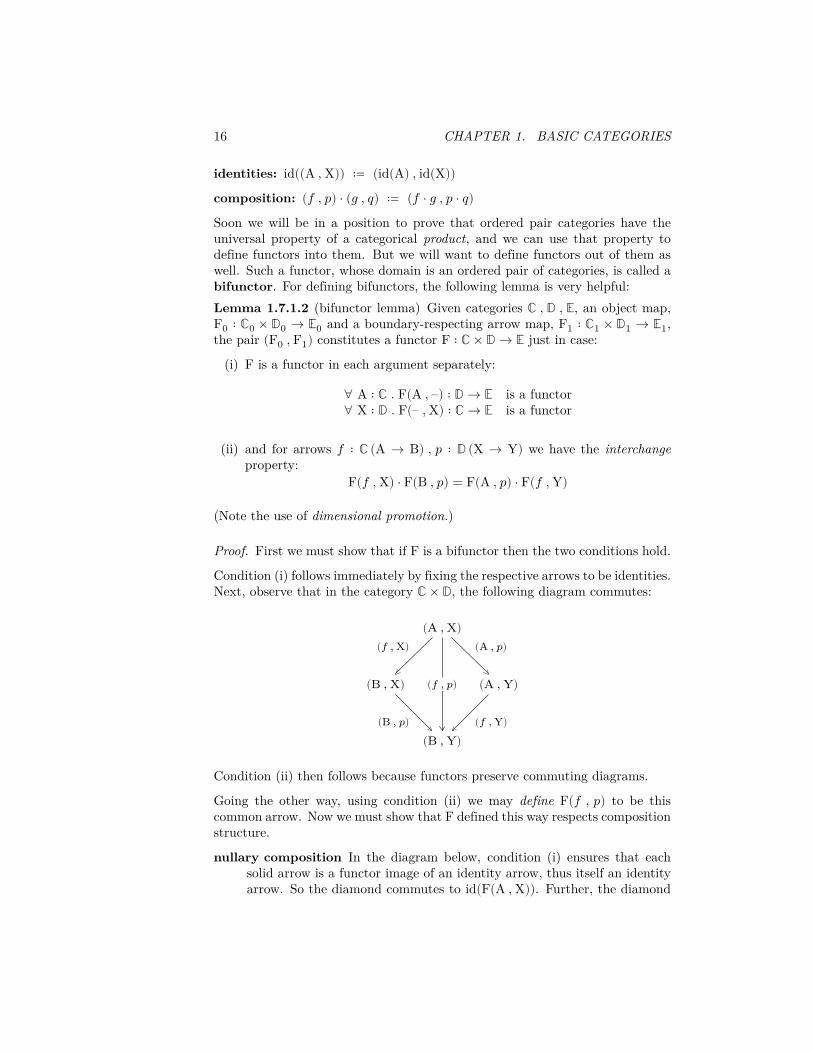
identities: id((A , X)) ≔ (id(A) , id(X))composition: (𝑓 , 𝑝) ⋅ (𝑔 , 𝑞) ≔ (𝑓 ⋅ 𝑔 , 𝑝 ⋅ 𝑞)Soon we will be in a position to prove that ordered pair categories have theuniversal property of a categorical product, and we can use that property todefine functors into them. But we will want to define functors out of them aswell. Such a functor, whose domain is an ordered pair of categories, is called abifunctor. For defining bifunctors, the following lemma is very helpful:Lemma 1.7.1.2 (bifunctor lemma) Given categories ℂ , 𝔻 , 𝔼, an object map,F0 ∶ ℂ0 × 𝔻0 → 𝔼0 and a boundary-respecting arrow map, F1 ∶ ℂ1 × 𝔻1 → 𝔼1,the pair (F0 , F1) constitutes a functor F ∶ ℂ × 𝔻 → 𝔼 just in case:
(i) F is a functor in each argument separately:
∀ A ∶ ℂ . F(A , –) ∶ 𝔻 → 𝔼 is a functor∀ X ∶ 𝔻 . F(– , X) ∶ ℂ → 𝔼 is a functor
(ii) and for arrows 𝑓 ∶ ℂ (A → B) , 𝑝 ∶ 𝔻 (X → Y) we have the interchangeproperty:
F(𝑓 , X) ⋅ F(B , 𝑝) = F(A , 𝑝) ⋅ F(𝑓 , Y)
(Note the use of dimensional promotion.)
Proof. First we must show that if F is a bifunctor then the two conditions hold.
Condition (i) follows immediately by fixing the respective arrows to be identities.Next, observe that in the category ℂ × 𝔻, the following diagram commutes:
(A , X)
(B , X) (A , Y)
(B , Y)
(𝑓 , X) (A , 𝑝)
(B , 𝑝) (𝑓 , Y)
(𝑓 , 𝑝)
Condition (ii) then follows because functors preserve commuting diagrams.
Going the other way, using condition (ii) we may define F(𝑓 , 𝑝) to be thiscommon arrow. Now we must show that F defined this way respects compositionstructure.
nullary composition In the diagram below, condition (i) ensures that eachsolid arrow is a functor image of an identity arrow, thus itself an identityarrow. So the diamond commutes to id(F(A , X)). Further, the diamond

1.7. NEW CATEGORIES FROM OLD 17
has the form described in condition (ii), so the defined map, F(id , id), isindeed the identity.
F(A , X)
F(A , X) F(A , X)
F(A , X)
F(id , X) F(A , id)
F(A , id) F(id , X)
F(id , id)
binary composition In the diagram below, each of the four diamonds com-mutes by condition (ii), giving us the defined maps F(𝑓 , 𝑝) and F(𝑔 , 𝑞) asshown. By condition (i) each of the four outer triangles commutes, so bycondition (ii) we have the defined map F(𝑓 ⋅ 𝑔 , 𝑝 ⋅ 𝑞) ∶ F(A , X) → F(C , Z).By pasting, the whole diagram commutes, so F preserves composites asdesired.
F(A , X)
F(B , X) F(A , Y)
F(C , X) F(B , Y) F(A , Z)
F(C , Y) F(B , Z)
F(C , Z)
F(𝑓 ⋅ 𝑔 , X) F(A , 𝑝 ⋅ 𝑞)
F(C , 𝑝 ⋅ 𝑞) F(𝑓 ⋅ 𝑔 , Z)
F(𝑓 , X) F(A , 𝑝)
F(B , 𝑝) F(𝑓 , Y)
F(𝑓 , 𝑝)
F(𝑔 , Y) F(B , 𝑞)
F(C , 𝑞) F(𝑔 , Z)F(𝑔 , 𝑞)
F(𝑔 , X)
F(C , 𝑝)
F(A , 𝑞)
F(𝑝 , Z)
1.7.2 Subcategories
Just as we may restrict our attention to a subset of a given set, we may singleout a substructure of a category as well. However, since a category has morestructure than a set, we must ensure that the substructure in question remainsa category.

18 CHAPTER 1. BASIC CATEGORIES
Definition 1.7.2.1 (subcategory) Given a category ℂ, we may take a subcat-egory 𝔻 of ℂ, written “𝔻 ⊆ ℂ” by taking for 𝔻0 a subcollection of ℂ0 and for𝔻1 a subcollection of ℂ1, subject to the restrictions:
• if 𝑓 ∶∶ ℂ is in 𝔻1 then ∂−(𝑓) and ∂+(𝑓) are in 𝔻0.
• if 𝑓 , 𝑔 ∶∶ ℂ are in 𝔻1 and are composable in ℂ then 𝑓 ⋅ 𝑔 is in 𝔻1.
• if A ∶ ℂ is in 𝔻0 then id(A) is in 𝔻1.
The composition structure of arrows when interpreted in 𝔻 is the same as in ℂ.
The restrictions are necessary to ensure that the subcollections of ℂ0 and ℂ1 wechoose do, in fact, form a category.
Whenever we have a subcategory 𝔻 ⊆ ℂ, we have also an inclusion functor𝑖 ∶ 𝔻 → ℂ, written “𝔻 ↪ ℂ”, sending each object and arrow of 𝔻 to itself, butnow viewed as an object or arrow of ℂ.
1.7.3 Opposite Categories
Recall that each arrow in a category has two boundary objects, its domain andcodomain. Systematically swapping these gives rise to an involutive relation oncategories.Definition 1.7.3.1 (opposite category) To any category ℂ, there correspondsan opposite category, ℂ° (pronounced “ℂ-op”), having:
objects: ℂ°0 ≔ ℂ0
arrows: ℂ° (A → B) ≔ ℂ (B → A)identities: id(A) ∶∶ ℂ° ≔ id(A) ∶∶ ℂcomposition: 𝑓 ⋅ 𝑔 ∶∶ ℂ° ≔ 𝑔 ⋅ 𝑓 ∶∶ ℂExercise 1.7.3.2 Check that an opposite category satisfies the unit and asso-ciative laws of composition, and that the opposite of an opposite category isjust the original category.
Despite being simple and purely formal, the opposite category construction isvery useful. Because it is an involution (for any category ℂ, we have that(ℂ°)° = ℂ), op is called a duality.
For any construction that we may perform in a given category, we can viewit from the perspective of the opposite category instead. this determines adual construction. In some cases a construction and its dual may arise withinthe same category and interact in interesting ways (as, for example with thedistributive law).
Furthermore, for any proposition that we may state about a given category,there is a dual proposition about its opposite category that is true just in
1.7. NEW CATEGORIES FROM OLD 19
case the first proposition is true of the original category. This gives us dualtheorems for free: in category theory theorems are always two for the proof ofone!
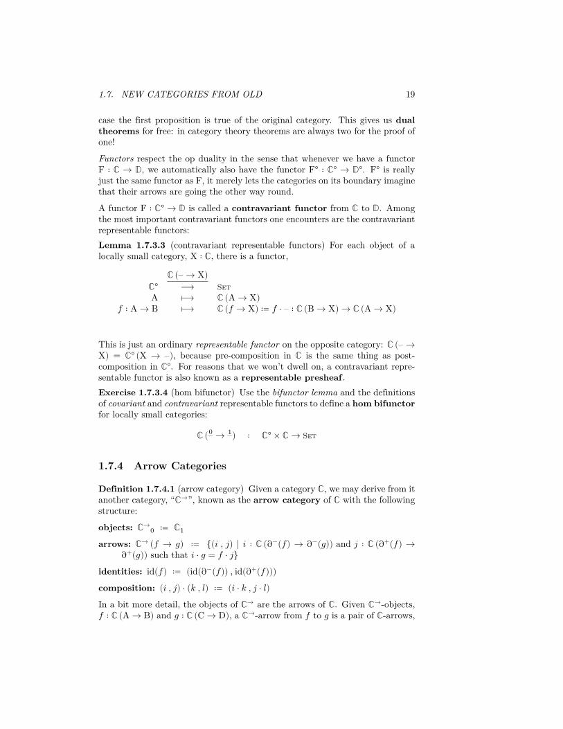
Functors respect the op duality in the sense that whenever we have a functorF ∶ ℂ → 𝔻, we automatically also have the functor F° ∶ ℂ° → 𝔻°. F° is reallyjust the same functor as F, it merely lets the categories on its boundary imaginethat their arrows are going the other way round.
A functor F ∶ ℂ° → 𝔻 is called a contravariant functor from ℂ to 𝔻. Amongthe most important contravariant functors one encounters are the contravariantrepresentable functors:Lemma 1.7.3.3 (contravariant representable functors) For each object of alocally small category, X ∶ ℂ, there is a functor,
ℂ (– → X)ℂ° ⟶ SetA ⟼ ℂ (A → X)
𝑓 ∶ A → B ⟼ ℂ (𝑓 → X) ≔ 𝑓 ⋅ – ∶ ℂ (B → X) → ℂ (A → X)
This is just an ordinary representable functor on the opposite category: ℂ (– →X) = ℂ° (X → –), because pre-composition in ℂ is the same thing as post-composition in ℂ°. For reasons that we won’t dwell on, a contravariant repre-sentable functor is also known as a representable presheaf .Exercise 1.7.3.4 (hom bifunctor) Use the bifunctor lemma and the definitionsof covariant and contravariant representable functors to define a hom bifunctorfor locally small categories:
ℂ (0– → 1–) ∶ ℂ° × ℂ → Set
1.7.4 Arrow Categories
Definition 1.7.4.1 (arrow category) Given a category ℂ, we may derive from itanother category, “ℂ→”, known as the arrow category of ℂ with the followingstructure:
objects: ℂ→0 ≔ ℂ1
arrows: ℂ→ (𝑓 → 𝑔) ≔ {(𝑖 , 𝑗) | 𝑖 ∶ ℂ (∂−(𝑓) → ∂−(𝑔)) and 𝑗 ∶ ℂ (∂+(𝑓) →∂+(𝑔)) such that 𝑖 ⋅ 𝑔 = 𝑓 ⋅ 𝑗}
identities: id(𝑓) ≔ (id(∂−(𝑓)) , id(∂+(𝑓)))composition: (𝑖 , 𝑗) ⋅ (𝑘 , 𝑙) ≔ (𝑖 ⋅ 𝑘 , 𝑗 ⋅ 𝑙)In a bit more detail, the objects of ℂ→ are the arrows of ℂ. Given ℂ→-objects,𝑓 ∶ ℂ (A → B) and 𝑔 ∶ ℂ (C → D), a ℂ→-arrow from 𝑓 to 𝑔 is a pair of ℂ-arrows,

20 CHAPTER 1. BASIC CATEGORIES
𝑖 ∶ ℂ (A → C) and 𝑗 ∶ ℂ (B → D) that form a commuting square with 𝑓 and 𝑔in ℂ:
A C
B D𝑓 𝑔
𝑖
𝑗
(1.1)
Identity ℂ→-arrows are the commuting ℂ-squares with two opposite sides thesame arrow and the other two opposite sides identity arrows. Composition inℂ→ is the pasting of commuting squares in ℂ:
A A
B B𝑓 𝑓
id
id
A C E
B D F𝑓 𝑔 ℎ
𝑖
𝑗
𝑘
𝑙
The unit and associative laws of composition are satisfied in ℂ→ as a consequenceof their holding in ℂ (you should check this). So the arrows of ℂ→ are thecommuting squares of ℂ (with each commuting ℂ-square represented twice).This tells us something about the 2-dimensional structure of ℂ, namely, whichof its squares commute.
We can iterate this construction to explore yet higher-dimensional structureof ℂ. One dimension up, the category (ℂ→)→ has as objects ℂ→-arrows (i.e.ℂ-commuting squares) and as arrows ℂ→-commuting squares. Let’s see whatthese ought to be. A nice way to think about it is to take diagram (1.1) andimagine that it’s actually a 3-dimensional cube that we happen to be seeingorthographically along one face. If we shift our perspective slightly, we will seethe following:
•
•
•
•
•
•
•
•
𝑓0 𝑔0
𝑖0
𝑗0
𝑓1 𝑔1
𝑖1
𝑗1
𝑎
𝑏
𝑐
𝑑
(1.2)
We begin with (ℂ→)→-objects 𝑓 and 𝑔, which are actually the ℂ→-arrows from 𝑎to 𝑏 and from 𝑐 to 𝑑, respectively. These, in turn, are the ℂ-commuting squaresshown on the left and right of diagram (1.2). Now (ℂ→)→-arrows between thesewill be ℂ→-arrows between their domains and codomains, 𝑖 and 𝑗, which arethe ℂ-commuting squares shown on the top and bottom. But there is also thecondition that 𝑖⋅𝑔 = 𝑓 ⋅𝑗 in ℂ→. Composition in ℂ→ is pasting in ℂ, and equalityof arrows in ℂ→ is just pairwise equality in ℂ. So we need that 𝑖0 ⋅𝑔0 = 𝑓0 ⋅𝑗0 and𝑖1 ⋅ 𝑔1 = 𝑓1 ⋅ 𝑗1 in ℂ, making the back and front faces commute. In other words,
1.7. NEW CATEGORIES FROM OLD 21
the top and bottom commuting ℂ-squares form a (ℂ→)→-arrow between theleft and right commuting ℂ-squares just in case the front and back ℂ-squarescommute as well. Then all the paths shown in diagram (1.2) commute. So(ℂ→)→-arrows are ℂ-commuting cubes.
The arrow category construction provides us with three important functors, thatin a sense “mediate between dimensions”. These are the domain, reflexivityand codomain functors:
𝑑𝑜𝑚ℂ→ ⟶ ℂ
𝑓 ∶∶ ℂ ⟼ ∂−(𝑓)(𝑖 , 𝑗) ⟼ 𝑖
𝑟𝑒𝑓𝑙ℂ ⟶ ℂ→
A ⟼ id(A)𝑓 ⟼ (𝑓 , 𝑓)
𝑐𝑜𝑑ℂ→ ⟶ ℂ
𝑓 ∶∶ ℂ ⟼ ∂+(𝑓)(𝑖 , 𝑗) ⟼ 𝑗
We will see later that these functors play an important role in the higher-dimensional structure of categories, but for now we will use the codomain functorto construct another important new category from old.
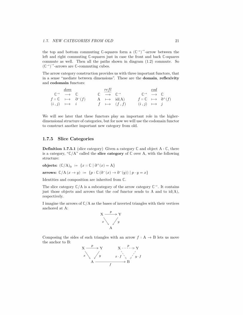
1.7.5 Slice Categories
Definition 1.7.5.1 (slice category) Given a category ℂ and object A ∶ ℂ, thereis a category, “ℂ/A” called the slice category of ℂ over A, with the followingstructure:
objects: (ℂ/A)0 ≔ {𝑥 ∶∶ ℂ | ∂+(𝑥) = A}arrows: ℂ/A (𝑥 → 𝑦) ≔ {𝑝 ∶ ℂ (∂−(𝑥) → ∂−(𝑦)) | 𝑝 ⋅ 𝑦 = 𝑥}Identities and composition are inherited from ℂ.
The slice category ℂ/A is a subcategory of the arrow category ℂ→. It containsjust those objects and arrows that the 𝑐𝑜𝑑 functor sends to A and to id(A),respectively.
I imagine the arrows of ℂ/A as the bases of inverted triangles with their verticesanchored at A:
X Y
A𝑥 𝑦
𝑝
Composing the sides of such triangles with an arrow 𝑓 ∶ A → B lets us movethe anchor to B:
X Y X Y
A B𝑓
𝑥 𝑦
𝑝
𝑥 ⋅ 𝑓 𝑦 ⋅ 𝑓
𝑝

22 CHAPTER 1. BASIC CATEGORIES
Lemma 1.7.5.2 (post-composition functor) Every arrow 𝑓 ∶ ℂ (A → B) deter-mines a functor:
𝑓!ℂ/A ⟶ ℂ/B
𝑥 ∶ ℂ (X → A) ⟼ 𝑥 ⋅ 𝑓𝑝 ∶ ℂ (X → Y) ⟼ 𝑝
Chapter 2
Behavioral Reasoning
A fundamental question we must address when studying any kind of formalsystem is when two objects with distinct presentations should be considered tobe essentially the same. We can ask this question about sets, groups, topologicalspaces, λ-terms, and even categories.
Certainly, whatever relation we choose should be an equivalence relation andshould be a congruence for certain operations, but beyond that, general guide-lines are hard to come by.
For example, we consider two sets to be essentially the same if there is a bijec-tion between them, that is, if there is an injective and surjective function fromone to the other. Recall that a function 𝑝 ∶ X → Y is injective if it “doesn’tcollapse any elements of its domain”:
∀ 𝑥0 , 𝑥1 ∈ X . 𝑝(𝑥0) = 𝑝(𝑥1) ⊃ 𝑥0 = 𝑥1
and is surjective if it “doesn’t miss any elements of its codomain”:
∀ 𝑦 ∈ Y . ∃ 𝑥 ∈ X . 𝑝(𝑥) = 𝑦
We can’t translate such element-wise definitions directly to the language ofcategories because the objects of a category need not be structured sets, so wemust find equivalent behavioral characterizations.
2.1 Monic and Epic Morphisms
2.1.1 Monomorphisms
In the case of injections, we can do this by rephrasing the property so thatrather than discussing the image under 𝑝 of two points of X, we instead discuss
23

24 CHAPTER 2. BEHAVIORAL REASONING
the composition with 𝑝 of two parallel functions into X. If 𝑝 is injective then:
∀ 𝑓 , 𝑔 ∶ W → X . ∀ 𝑤 ∈ W . (𝑝 ∘ 𝑓)(𝑤) = (𝑝 ∘ 𝑔)(𝑤) ⊃ 𝑓(𝑤) = 𝑔(𝑤)
Universal quantification distributes over implication, i.e. if ∀𝑎 ∶ A . φ 𝑎 ⊃ ψ 𝑎then (∀𝑎 ∶ A . φ 𝑎) ⊃ (∀𝑎 ∶ A . ψ 𝑎). Thus if 𝑝 is injective then:
∀ 𝑓 ,𝑔 ∶ W → X . (∀ 𝑤 ∈ W . (𝑝∘𝑓)(𝑤) = (𝑝∘𝑔)(𝑤)) ⊃ (∀ 𝑤 ∈ W . 𝑓(𝑤) = 𝑔(𝑤))
It may seem that we’ve just made things worse by introducing two extraneousfunctions, but now we can use the fact that two functions are equal just incase they agree on all points to rephrase this again, doing away with the pointsentirely. So if 𝑝 is injective then:
∀ 𝑓 , 𝑔 ∶ W → X . 𝑓 ⋅ 𝑝 = 𝑔 ⋅ 𝑝 ⊃ 𝑓 = 𝑔
This is a behavioral characterization that can be stated for any category.Definition 2.1.1.1 (monomorphism) An arrow 𝑚 ∶∶ ℂ is a monomorphism(or “monic”) if it is post-cancelable; that is, if for any arrows 𝑓 , 𝑔 ∶∶ ℂ,
𝑓 ⋅ 𝑚 = 𝑔 ⋅ 𝑚 implies 𝑓 = 𝑔
Notice that we are being a bit economical here: in order for 𝑓 and 𝑔 to becomposable with 𝑚, they must be coterminal, and in order for their compositeswith 𝑚 to be equal, they must also be coinitial. So the implication is applicableonly to parallel 𝑓 and 𝑔 composable with 𝑚, but all that can be inferred.
In diagrams, monomorphisms are conventionally drawn with a tailed arrow:“↣”.Lemma 2.1.1.2 (monics and composition)
• Identity morphisms are monic.
• Composites of monics are monic.
• If the composite 𝑚 ⋅ 𝑛 is monic then so is 𝑚.
Proof.
𝑓 ⋅ id = 𝑔 ⋅ id⇒ [unit law]
𝑓 = 𝑔
𝑓 ⋅ 𝑚 ⋅ 𝑛 = 𝑔 ⋅ 𝑚 ⋅ 𝑛⇒ [𝑛 is monic]
𝑓 ⋅ 𝑚 = 𝑔 ⋅ 𝑚⇒ [𝑚 is monic]
𝑓 = 𝑔
𝑓 ⋅ 𝑚 = 𝑔 ⋅ 𝑚⇒ [whiskering]
𝑓 ⋅ 𝑚 ⋅ 𝑛 = 𝑔 ⋅ 𝑚 ⋅ 𝑛⇒ [𝑚 ⋅ 𝑛 is monic]
𝑓 = 𝑔
2.1. MONIC AND EPIC MORPHISMS 25
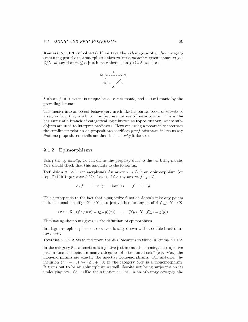
Remark 2.1.1.3 (subobjects) If we take the subcategory of a slice categorycontaining just the monomorphisms then we get a preorder: given monics 𝑚,𝑛 ∶ℂ/A, we say that 𝑚 ≤ 𝑛 just in case there is an 𝑓 ∶ ℂ/A (𝑚 → 𝑛).
M N
A𝑚 𝑛
𝑓
Such an 𝑓 , if it exists, is unique because 𝑛 is monic, and is itself monic by thepreceding lemma.
The monics into an object behave very much like the partial order of subsets ofa set, in fact, they are known as (representatives of) subobjects. This is thebeginning of a branch of categorical logic known as topos theory, where sub-objects are used to interpret predicates. However, using a preorder to interpretthe entailment relation on propositions sacrifices proof relevance: it lets us saythat one proposition entails another, but not why it does so.
2.1.2 Epimorphisms
Using the op duality, we can define the property dual to that of being monic.You should check that this amounts to the following:Definition 2.1.2.1 (epimorphism) An arrow 𝑒 ∶∶ ℂ is an epimorphism (or“epic”) if it is pre-cancelable; that is, if for any arrows 𝑓 , 𝑔 ∶∶ ℂ,
𝑒 ⋅ 𝑓 = 𝑒 ⋅ 𝑔 implies 𝑓 = 𝑔
This corresponds to the fact that a surjective function doesn’t miss any pointsin its codomain, so if 𝑝 ∶ X → Y is surjective then for any parallel 𝑓 , 𝑔 ∶ Y → Z,
(∀𝑥 ∈ X . (𝑓 ∘ 𝑝)(𝑥) = (𝑔 ∘ 𝑝)(𝑥)) ⊃ (∀𝑦 ∈ Y . 𝑓(𝑦) = 𝑔(𝑦))
Eliminating the points gives us the definition of epimorphism.
In diagrams, epimorphisms are conventionally drawn with a double-headed ar-row: “↠”.Exercise 2.1.2.2 State and prove the dual theorems to those in lemma 2.1.1.2.
In the category Set a function is injective just in case it is monic, and surjectivejust in case it is epic. In many categories of “structured sets” (e.g. Mon) themonomorphisms are exactly the injective homomorphisms. For instance, theinclusion (ℕ , + , 0) ↪ (ℤ , + , 0) in the category Mon is a monomorphism.It turns out to be an epimorphism as well, despite not being surjective on itsunderlying set. So, unlike the situation in Set, in an arbitrary category the

26 CHAPTER 2. BEHAVIORAL REASONING
existence of a monic and epic morphism between two objects does not suffice toensure that they are essentially the same.
Monic and epic morphisms have other unsatisfactory properties, for example,they are not necessarily preserved by functors (the existence of a forgetful functorfrom monoids to sets, together with the last result implies this).
2.2 Split Monic and Epic Morphisms
Definition 2.2.0.1 (split monomorphism) An arrow 𝑠 is a split monomor-phism (or “split monic”) if it is post-(semi-)invertible; that is, if there exists anarrow 𝑟 such that 𝑠 ⋅ 𝑟 = id.
The dual notion is that of:Definition 2.2.0.2 (split epimorphism) An arrow 𝑟 is a split epimorphism(or “split epic”) if it is pre-(semi-)invertible; that is, if there exists an arrow 𝑠such that 𝑠 ⋅ 𝑟 = id.
It would be perverse to name them this way unless split monics were monic andsplit epics were epic, which indeed they are.Lemma 2.2.0.3 A split monomorphism is a monomorphism (and a split epi-morphism is an epimorphism).
Proof. Suppose 𝑠 is split-monic with 𝑠 ⋅ 𝑟 = id,
𝑓 ⋅ 𝑠 = 𝑔 ⋅ 𝑠⟹ [whiskering]
𝑓 ⋅ 𝑠 ⋅ 𝑟 = 𝑔 ⋅ 𝑠 ⋅ 𝑟⟹ [assumption]
𝑓 ⋅ id = 𝑔 ⋅ id⟹ [unit law]
𝑓 = 𝑔
The other case is dual.
Because functors must preserve the composition structure of categories, theymust preserve split monics and epics as well.Lemma 2.2.0.4 The functor-image of a split monic (split epic) is itself splitmonic (split epic).

2.2. SPLIT MONIC AND EPIC MORPHISMS 27
Proof. Suppose 𝑠 is split-monic with 𝑠 ⋅ 𝑟 = id,
F(𝑠) ⋅ F(𝑟)= [functors preserve composition]
F(𝑠 ⋅ 𝑟)= [assumption]
F(id)= [functors preserve identities]
id
So F(𝑠) is split-monic.
Before moving on, let’s consider a particularly pretty application of behavioralreasoning to the axiom of choice. This proposition states that given a family ofnon-empty sets, there is a function that chooses an element from each one.
We can represent any family of sets with an ordinary function in the followingway. Given a function 𝑓 ∶ Set (E → B), we can define a function,
𝑓∗
B ⟶ ℘(E) ↪ Set𝑏 ⟼ {𝑒 ∈ E | 𝑓(𝑒) = 𝑏}
And given a family of sets, {E𝑏}𝑏∈B, which is just an map B → Set, we candefine a projection function ∫𝑏∈B E𝑏 → B mapping 𝑒 ∈ E𝑏 ⟼ 𝑏. These twoconstructions are inverse, both the function 𝑓 ∶ E → B and the family of sets{E𝑏}𝑏∈B just sort the elements of E by those in B:
B
E
B
℘(E)
● ● ●
● ● ● ● ●
𝑓 𝑓∗
The axiom of choice states that if for each 𝑏 ∈ B the set 𝑓∗(𝑏) is non-emptythen there is a way to choose from E a family of elements {𝑒𝑏}𝑏∈B such that∀ 𝑏 ∈ B . 𝑓(𝑒𝑏) = 𝑏 – i.e. such that there is a function 𝑠 ∶ B → E with𝑠 ⋅ 𝑓 = id(B). Notice that the condition that the sets 𝑓∗(𝑏) be non-empty isequivalent to the requirement that 𝑓 be a surjection. So the axiom of choiceasserts that in the category Set, every epimorphism is split!
This is a behavioral characterization of a property that we may ask whether agiven category satisfies. For example, because the inclusion (ℕ,+,0) ↪ (ℤ,+,0)is epic in the category Mon, it fails to hold there.
28 CHAPTER 2. BEHAVIORAL REASONING
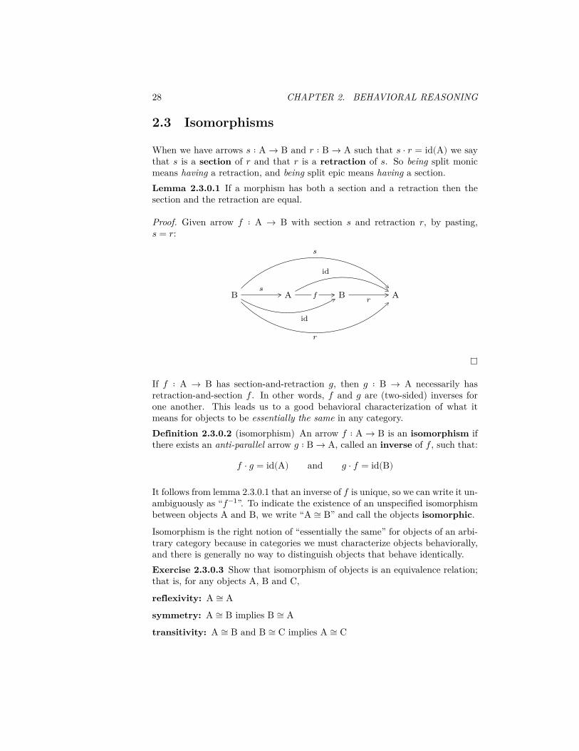
2.3 Isomorphisms
When we have arrows 𝑠 ∶ A → B and 𝑟 ∶ B → A such that 𝑠 ⋅ 𝑟 = id(A) we saythat 𝑠 is a section of 𝑟 and that 𝑟 is a retraction of 𝑠. So being split monicmeans having a retraction, and being split epic means having a section.Lemma 2.3.0.1 If a morphism has both a section and a retraction then thesection and the retraction are equal.
Proof. Given arrow 𝑓 ∶ A → B with section 𝑠 and retraction 𝑟, by pasting,𝑠 = 𝑟:
B A B A𝑠
𝑓 𝑟
id
id
𝑠
𝑟
If 𝑓 ∶ A → B has section-and-retraction 𝑔, then 𝑔 ∶ B → A necessarily hasretraction-and-section 𝑓 . In other words, 𝑓 and 𝑔 are (two-sided) inverses forone another. This leads us to a good behavioral characterization of what itmeans for objects to be essentially the same in any category.Definition 2.3.0.2 (isomorphism) An arrow 𝑓 ∶ A → B is an isomorphism ifthere exists an anti-parallel arrow 𝑔 ∶ B → A, called an inverse of 𝑓 , such that:
𝑓 ⋅ 𝑔 = id(A) and 𝑔 ⋅ 𝑓 = id(B)
It follows from lemma 2.3.0.1 that an inverse of 𝑓 is unique, so we can write it un-ambiguously as “𝑓−1”. To indicate the existence of an unspecified isomorphismbetween objects A and B, we write “A ≅ B” and call the objects isomorphic.
Isomorphism is the right notion of “essentially the same” for objects of an arbi-trary category because in categories we must characterize objects behaviorally,and there is generally no way to distinguish objects that behave identically.Exercise 2.3.0.3 Show that isomorphism of objects is an equivalence relation;that is, for any objects A, B and C,
reflexivity: A ≅ Asymmetry: A ≅ B implies B ≅ Atransitivity: A ≅ B and B ≅ C implies A ≅ C

2.3. ISOMORPHISMS 29
Definition 2.3.0.4 (groupoid) A category in which every arrow is an isomor-phism is called a groupoid. In particular, a single-object groupoid is a group.Exercise 2.3.0.5 Check that this definition coincides with the usual definitionof a group.

30 CHAPTER 2. BEHAVIORAL REASONING

Chapter 3
Universal Constructions
A universal construction is a description of a construction within a categorythat determines it uniquely up to a canonical isomorphism. This is the bestkind of description we can hope for in a behavioral setting, where we do nothave direct access to the internal structure of the objects we are working with.
Universal constructions are defined using universal properties, which assertthat the construction itself has some property, and that if any other constructionin the category has the same property then there is a canonical relationshipbetween the two.
In this chapter we introduce the universal constructions needed for the cate-gorical interpretation of typing contexts and simple type formers. We do thisin a deliberately methodical way, in order to emphasize the similarities in theconstructions.
3.1 Terminal and Initial Objects
3.1.1 Terminal Objects
In the category Set, a singleton set S has the property that given any set Xthere is a unique function from X to S, namely, the constant function on theonly element of S. This is a behavioral characterization that we may state inan arbitrary category.Definition 3.1.1.1 (terminal object) In any category, a terminal object is anobject T with the property that for any object X there is a unique morphism𝑥 ∶ X → T.
We write “!(X)” for the unique map from an object X to a terminal object andrefer to it as a bang map.
31

32 CHAPTER 3. UNIVERSAL CONSTRUCTIONS
Whenever some construction has a certain relationship to all constructions ofthe same kind within a category, it must, in particular, have this relationshipto itself. Socrates’ dictum to “know thyself” is as important in category theoryas it is in life. So whenever we encounter a universal construction we will seewhat we can learn about it by “probing it with itself”. In the case of a terminalobject, this means choosing X ≔ T in the definition.Lemma 3.1.1.2 (identity expansion for terminals) If T is a terminal objectthen !(T) = id(T).
Proof. By assumption, !(T) is the unique map 𝑡 ∶ T → T, but id(T) is an arrowin the same hom set.
Universal constructions are each unique up to a unique structure-preservingisomorphism. In the case of a terminal object, the structure to be preserved istrivial: it’s just a single object. Consequently, we obtain an especially stronguniqueness property.Lemma 3.1.1.3 (uniqueness of terminals) When they exist, terminal objectsare unique up to a unique isomorphism.
Proof. Suppose that T and R are two terminal objects in a category. By as-sumption, there are unique arrows 𝑡 ∶ T → R and 𝑟 ∶ R → T and:
𝑡 ⋅ 𝑟 ∶ T → T= [T is terminal]
!(T) ∶ T → T= [identity expansion for terminals]
id(T) ∶ T → T
R
T T
𝑡 𝑟
!
id
Symmetrically, we have that 𝑟 ⋅ 𝑡 = id(R). So 𝑡 is an isomorphism. By theuniversal property of R, the hom set T → R is a singleton, so it must be theonly one.
Because terminal objects are unique up to unique isomorphism, we write “1” torefer to an arbitrary terminal object of a category.

3.1. TERMINAL AND INITIAL OBJECTS 33
Exercise 3.1.1.4 (pre-composing with a bang) Use the universal property of aterminal object to prove the following:
For a terminal object 1 and arrow 𝑖 ∶ Y → X,
𝑖 ⋅ !(X) = !(Y) ∶ Y → 1
Y X
1!!
𝑖
As mentioned, in SET, any singleton set is terminal. Likewise, in Cat, anysingleton category is. In Mon, the trivial monoid (having only the identityelement) is terminal.Exercise 3.1.1.5 Work out what a terminal object is in the category PreOrd,and determine when a preordered set, as a category, has a terminal object.
3.1.2 Unit Type
The terminal object universal construction provides a categorical interpretationof the unit type, ⊤,
⟦⊤⟧ ≔ 1The introduction rule for unit type,
Γ ⊢ ⋆ ∶ ⊤ ⊤+
is interpreted by the bang map:
⟦⋆⟧ ≔ !(⟦Γ⟧) ∶ ⟦Γ⟧ → 1
3.1.3 Global and Generalized Elements
In Set, there is a bijection between the elements of a set X and the functionsfrom a singleton set to X: to each 𝑥 ∈ X there corresponds the unique function⌜𝑥⌝ ∶ 1 → X mapping ⋆ ⟼ 𝑥. We can use this behavioral characterization todefine an analogue for set membership.Definition 3.1.3.1 (global element) In a category with a terminal object, aglobal element (or “point”) of an object X is an element of the hom set 1 → X.Definition 3.1.3.2 (generalized element) In contrast, a generalized elementof an object X is just a morphism with codomain X; in other words, an objectof the slice category over X.

34 CHAPTER 3. UNIVERSAL CONSTRUCTIONS
In Set, we can determine whether or not two functions are the same by probingthem with points because two parallel functions 𝑓 , 𝑔 ∶ Set (X → Y) are equaljust in case ∀𝑥 ∈ X . 𝑓(𝑥) = 𝑔(𝑥). This is known as the principle of functionextensionality. Here is a categorical analogue:Definition 3.1.3.3 (well-pointed category) A category with a terminal objectis well-pointed if for every 𝑓 , 𝑔 ∶ A → B, and global element 𝑎 ∶ 1 → A ,
𝑎 ⋅ 𝑓 = 𝑎 ⋅ 𝑔 implies 𝑓 = 𝑔
Notice the similarity to the definition of an epimorphism. In fact, we say thata category is well-pointed if its points are jointly epic, that is, if points arecollectively able to distinguish arrows.Exercise 3.1.3.4 In contrast to the case with global elements, in any categorywe can determine whether or not two parallel arrows are the same by probingthem with generalized elements. Prove this. (Hint: for any pair of arrows, asingle “probe” suffices.)
3.1.4 Initial Objects
The concept dual to that of a terminal object is of an initial object.Definition 3.1.4.1 (initial object) In any category, an initial object is anobject S with the property that for any object X there is a unique morphism𝑥 ∶ S → XWe write “¡(X)” for the unique map in S → X and refer to it as a cobang map.By probing an initial object with itself we obtain a result dual to lemma 3.1.1.2:Lemma 3.1.4.2 (identity expansion for initials) If S is an initial object then¡(S) = id(S).Exercise 3.1.4.3 (uniqueness of initials) Check that when they exist, initialobjects are unique up to a unique isomorphism.
We write “0” to refer to an arbitrary initial object of a category.Lemma 3.1.4.4 (post-composing with a cobang) dual to exercise 3.1.1.4:
For an initial object 0 and arrow 𝑖 ∶ X → Y,
¡(X) ⋅ 𝑖 = ¡(Y) ∶ 0 → Y
0
X Y
¡ ¡
𝑖

3.2. PRODUCTS 35
In Set, the empty set is initial. Likewise, in Cat, the empty category is. InMon, the trivial monoid is initial as well as terminal. (An object which is bothterminal and initial is known as a null object.)Exercise 3.1.4.5 Dualize exercise 3.1.1.5 by working out what an initial objectis in the category PreOrd, and determine when a preordered set, as a category,has an initial object.
3.1.5 Void Type
The initial object universal construction provides a possible categorical inter-pretation of the void type, ⊥,
⟦⊥⟧ ≔ 0
In the restricted setting where contexts are singletons, the elimination rule forvoid type,
𝑧 ∶ ⊥ ⊢ abort† ∶ A⊥−†
is then interpreted by the cobang map:
⟦abort†⟧ ≔ ¡(⟦A⟧) ∶ 0 → ⟦A⟧
Note that in this case, the interpretations of all terms of a given type in aninconsistent context coincide:
∀(𝑧 ∶ ⊥ ⊢ M , N ∶ A) . ⟦M⟧ ≅ ⟦N⟧
Depending on how the type theory is set up, this equation may or may not bereflected there.
3.2 Products
3.2.1 Products of Objects
The set of ordered pairs:
A × B ≔ {(𝑎 , 𝑏) | 𝑎 ∈ A and 𝑏 ∈ B}
comes equipped with two projection functions,
π0A × B ⟶ A(𝑎 , 𝑏) ⟼ 𝑎 and
π1A × B ⟶ B(𝑎 , 𝑏) ⟼ 𝑏
36 CHAPTER 3. UNIVERSAL CONSTRUCTIONS
such that for ordered pair 𝑐 ∈ A × B,
𝑐 = (π0 𝑐 , π1 𝑐)
So having a pair of elements, one from the set A and one from the set B, is thesame thing as having a single element of the set A × B: given an 𝑎 ∈ A and𝑏 ∈ B we make an element of A × B by forming the tuple (𝑎 , 𝑏), and given anelement 𝑐 ∈ A × B we recover elements of A and B by taking the projections.
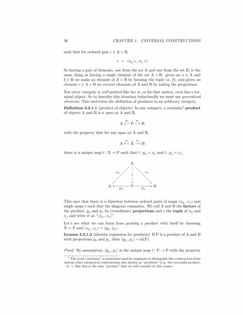
Not every category is well-pointed like Set is, or for that matter, even has a ter-minal object. So to describe this situation behaviorally we must use generalizedelements. This motivates the definition of products in an arbitrary category.Definition 3.2.1.1 (product of objects) In any category, a cartesian1 productof objects A and B is a span on A and B,
A𝑝0⟵ P
𝑝1⟶ B
with the property that for any span on A and B,
A𝑥0⟵ X
𝑥1⟶ B
there is a unique map 𝑡 ∶ X → P such that 𝑡 ⋅ 𝑝0 = 𝑥0 and 𝑡 ⋅ 𝑝1 = 𝑥1:
X
A P B𝑝0 𝑝1
𝑥0 𝑥1𝑡
This says that there is a bijection between ordered pairs of maps (𝑥0 , 𝑥1) andsingle maps 𝑡 such that the diagram commutes. We call A and B the factors ofthe product, 𝑝0 and 𝑝1 its (coordinate) projections and 𝑡 the tuple of 𝑥0 and𝑥1 and write it as “⟨𝑥0 , 𝑥1⟩”.Let’s see what we can learn from probing a product with itself by choosingX ≔ P and (𝑥0 , 𝑥1) ≔ (𝑝0 , 𝑝1).Lemma 3.2.1.2 (identity expansion for products) If P is a product of A and Bwith projections 𝑝0 and 𝑝1, then ⟨𝑝0 , 𝑝1⟩ = id(P).
Proof. By assumption, ⟨𝑝0 , 𝑝1⟩ is the unique map 𝑡 ∶ P → P with the property1 The word “cartesian” is sometimes used for emphasis to distinguish this construction from
various other categorical constructions also known as “products” (e.g. the monoidal product,– ⊗ –). But this is the only “product” that we will consider in this course.

3.2. PRODUCTS 37
that, 𝑡 ⋅ 𝑝0 = 𝑝0 and 𝑡 ⋅ 𝑝1 = 𝑝1:
P
A P B𝑝0 𝑝1
𝑝0 𝑝1⟨𝑝0 , 𝑝1⟩
but by the left unit law of composition, id(P) has this property.
Because products are structures characterized by a universal property, we ex-pect them to be uniquely determined up to a unique structure-preserving iso-morphism. This is indeed the case:Lemma 3.2.1.3 (uniqueness of products) When they exist, products of objectsare unique up to a unique projection-preserving isomorphism.
Proof. Suppose that the spans:
A𝑝0⟵ P
𝑝1⟶ B and A𝑞0⟵ Q
𝑞1⟶ B
are both products of A and B. Because Q is a product there is a unique 𝑠 ∶ P →Q such that 𝑠 ⋅ 𝑞0 = 𝑝0 and 𝑠 ⋅ 𝑞1 = 𝑝1. Likewise, because P is a product thereis a unique 𝑡 ∶ Q → P such that 𝑡 ⋅ 𝑝0 = 𝑞0 and 𝑡 ⋅ 𝑝1 = 𝑞1:
P
A Q B
P
𝑝0 𝑝1
𝑞0 𝑞1
𝑝0 𝑝1
𝑠
𝑡
Then for 𝑖 ∈ {0 , 1}:𝑠 ⋅ 𝑡 ⋅ 𝑝𝑖
= [P is a product]𝑠 ⋅ 𝑞𝑖
= [Q is a product]𝑝𝑖

38 CHAPTER 3. UNIVERSAL CONSTRUCTIONS
Thus 𝑠 ⋅ 𝑡 = ⟨𝑝0 , 𝑝1⟩ ∶ P → P. By identity expansion for products, 𝑠 ⋅ 𝑡 = id(P).Reversing the roles of P and Q, we get that 𝑡 ⋅ 𝑠 = id(Q) as well. So 𝑠 is anisomorphism. By the universal property of Q, it is the only one that respectsthe coordinate projections.
Because products are determined as uniquely as is possible by a behavioralcharacterization, we write “A × B” to refer to an arbitrary product of A andB. When the product in question is clear from context, we refer to the twocoordinate projections generically as “π0” and “π1”.
In the category Set, the set of ordered pairs is a cartesian product. Likewise, inCat, the ordered pair category is. This justifies the notation – × – that we usedin both cases.
Note that unlike the case with terminal objects, there is not necessarily a uniqueisomorphism between two products of the same factors. For example, in Set theidentity function, (𝑥 , 𝑦) ⟼ (𝑥 , 𝑦), and swap map, (𝑥 , 𝑦) ⟼ (𝑦 , 𝑥), are bothisomorphisms A × A → A × A. But only the former respects the coordinateprojections.Definition 3.2.1.4 (diagonal map) For every object A, the universal propertyof the product gives a canonical diagonal map, which duplicates its argument:
∆(A) ≔ ⟨id(A) , id(A)⟩ ∶ A → A × A
A
A A × A Aπ0 π1
id id∆
Exercise 3.2.1.5 (pre-composing with a tuple) Use the diagram below and theuniversal property of a product of objects to prove the following:
For a product A × B, a tuple ⟨𝑓 , 𝑔⟩ ∶ X → A × B and an arrow 𝑖 ∶ Y → X,
𝑖 ⋅ ⟨𝑓 , 𝑔⟩ = ⟨𝑖 ⋅ 𝑓 , 𝑖 ⋅ 𝑔⟩ ∶ Y → A × B
Y
X
A A × B Bπ0 π1
𝑓 𝑔⟨𝑓 , 𝑔⟩
𝑖𝑖 ⋅ 𝑓 𝑖 ⋅ 𝑔

3.2. PRODUCTS 39
3.2.2 Product Functors
We can use the universal property of a product of objects to define a productof arrows as well:Definition 3.2.2.1 (product of arrows) Given a pair of arrows 𝑓 ∶ X → A and𝑔 ∶ Y → B, and products X × Y and A × B, we define the product of arrowsby:
𝑓 × 𝑔 ∶ X × Y → A × B𝑓 × 𝑔 ≔ ⟨π0 ⋅ 𝑓 , π1 ⋅ 𝑔⟩
By the universal property of the product A × B, the arrow 𝑓 × 𝑔 is the uniquemorphism making the two squares commute:
X X × Y Y
A A × B B
π0 π1
π0 π1
𝑓 𝑔𝑓 × 𝑔
This allows us to characterize the product as a functor – indeed, a bifunctor:Lemma 3.2.2.2 (functoriality of products) If a category ℂ has products foreach pair of objects, then the given definition of products for arrows yields afunctor,
– × – ∶ ℂ × ℂ → ℂ
called the product functor.
Before giving the proof, we pause to explain this statement, as it is easy to beconfused about what is being asserted. In the theorem, “ℂ × ℂ” is the orderedpair category (definition 1.7.1.1); i.e. the product of ℂ with itself in Cat. Incontrast, “–×–” is the name of an alleged functor having as domain the categoryℂ × ℂ and as codomain the category ℂ.
Proof. In order to prove that – × – is a functor, we must show that it preservesthe composition structure.
nullary composition: We must show that
id(A0) × id(A1) = id(A0 × A1)

40 CHAPTER 3. UNIVERSAL CONSTRUCTIONS
In the diagram,
A0 A0 × A1 A1
A0 A0 × A1 A1
π0 π1
π0 π1
id idid
the arrow id(A0 × A1) makes both squares commute, so the result followsby the definition of product of arrows.
binary composition: We must show that
(𝑓0 ⋅ 𝑔0) × (𝑓1 ⋅ 𝑔1) = (𝑓0 × 𝑓1) ⋅ (𝑔0 × 𝑔1)
In the diagram,
A0 A0 × A1 A1
B0 B0 × B1 B1
C0 C0 × C1 C1
π0 π1
π0 π1
π0 π1
𝑓0 𝑓1
𝑔0 𝑔1
𝑓0 × 𝑓1
𝑔0 × 𝑔1
the top two squares commute by the definition of 𝑓0 × 𝑓1 and the bottomtwo squares commute by the definition of 𝑔0 × 𝑔1. By pasting, the rectan-gle comprising the two left squares commutes, and likewise the rectanglecomprising the two right squares. By definition, (𝑓0 ⋅ 𝑔0) × (𝑓1 ⋅ 𝑔1) is theunique arrow from A0 ×A1 to C0 ×C1 making the outer square commute.
Exercise 3.2.2.3 (post-composing a product of arrows) Use the universal prop-erty of a product of objects to prove the following:
For arrows ⟨𝑓0 , 𝑓1⟩ ∶ X → A0 × A1 and 𝑔0 × 𝑔1 ∶ A0 × A1 → B0 × B1,
⟨𝑓0 , 𝑓1⟩ ⋅ (𝑔0 × 𝑔1) = ⟨𝑓0 ⋅ 𝑔0 , 𝑓1 ⋅ 𝑔1⟩
3.2. PRODUCTS 41
X
A0 A0 × A1 A1
B0 B0 × B1 B1
π0 π1
π0 π1
𝑓0 𝑓1⟨𝑓0 , 𝑓1⟩
𝑔0 𝑔1𝑔0 × 𝑔1
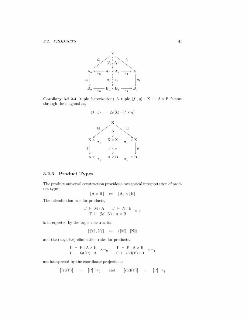
Corollary 3.2.2.4 (tuple factorization) A tuple ⟨𝑓 , 𝑔⟩ ∶ X → A × B factorsthrough the diagonal as,
⟨𝑓 , 𝑔⟩ = ∆(X) ⋅ (𝑓 × 𝑔)
X
X X × X X
A A × B B
π0 π1
π0 π1
id id∆
𝑓 𝑔𝑓 × 𝑔
3.2.3 Product Types
The product universal construction provides a categorical interpretation of prod-uct types,
⟦A × B⟧ ≔ ⟦A⟧ × ⟦B⟧The introduction rule for products,
Γ ⊢ M ∶ A Γ ⊢ N ∶ BΓ ⊢ ⟨M , N⟩ ∶ A × B ×+
is interpreted by the tuple construction:
⟦⟨M , N⟩⟧ ≔ ⟨⟦M⟧ , ⟦N⟧⟩
and the (negative) elimination rules for products,
Γ ⊢ P ∶ A × BΓ ⊢ fst(P) ∶ A
×−0Γ ⊢ P ∶ A × BΓ ⊢ snd(P) ∶ B
×−1
are interpreted by the coordinate projections:
⟦fst(P)⟧ ≔ ⟦P⟧ ⋅ π0 and ⟦snd(P)⟧ ≔ ⟦P⟧ ⋅ π1
42 CHAPTER 3. UNIVERSAL CONSTRUCTIONS
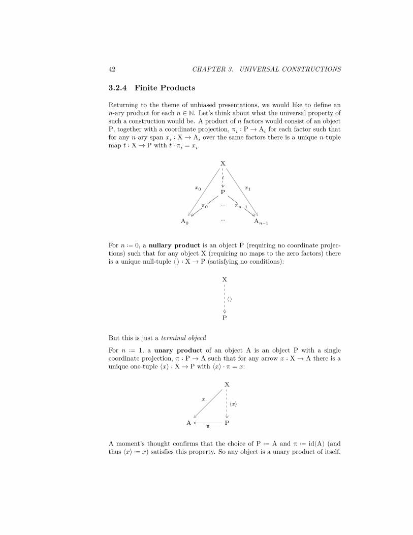
3.2.4 Finite Products
Returning to the theme of unbiased presentations, we would like to define an𝑛-ary product for each 𝑛 ∈ ℕ. Let’s think about what the universal property ofsuch a construction would be. A product of 𝑛 factors would consist of an objectP, together with a coordinate projection, π𝑖 ∶ P → A𝑖 for each factor such thatfor any 𝑛-ary span 𝑥𝑖 ∶ X → A𝑖 over the same factors there is a unique 𝑛-tuplemap 𝑡 ∶ X → P with 𝑡 ⋅ π𝑖 = 𝑥𝑖.
X
P
A0 A𝑛−1
π0 π𝑛−1
𝑥0 𝑥1
𝑡
⋯
⋯
For 𝑛 ≔ 0, a nullary product is an object P (requiring no coordinate projec-tions) such that for any object X (requiring no maps to the zero factors) thereis a unique null-tuple ⟨ ⟩ ∶ X → P (satisfying no conditions):
X
P
⟨ ⟩
But this is just a terminal object!
For 𝑛 ≔ 1, a unary product of an object A is an object P with a singlecoordinate projection, π ∶ P → A such that for any arrow 𝑥 ∶ X → A there is aunique one-tuple ⟨𝑥⟩ ∶ X → P with ⟨𝑥⟩ ⋅ π = 𝑥:
X
A Pπ
𝑥⟨𝑥⟩
A moment’s thought confirms that the choice of P ≔ A and π ≔ id(A) (andthus ⟨𝑥⟩ ≔ 𝑥) satisfies this property. So any object is a unary product of itself.

3.2. PRODUCTS 43
Binary products have already been defined, so we have left to consider productsof three or more factors. A ternary product is an object A × B × C, equippedwith three coordinate projection maps such that for any 3-legged span over itsfactors there is a unique map from the vertex to A × B × C commuting withthe coordinate projections. But this is the same universal property enjoyed by(A × B) × C, which has projections π0 ⋅ π0 to A, π0 ⋅ π1 to B and π1 to C. Anyspan over A, B and C contains a subspan over A and B, so by the universalproperty of A × B, has a unique map from the vertex to this product, whichtogether with the C leg of the span gives us a unique map from the vertex to(A × B) × C. The product of four or more factors is analogous.
Of course, there is nothing special about the choice of bracketing:Lemma 3.2.4.1 (product associator) Products are associative, up to isomor-phism:
A × (B × C) ≅ (A × B) × C
Proof. The maps back and forth,
𝑠 ∶ A × (B × C) → (A × B) × C and 𝑡 ∶ (A × B) × C → A × (B × C)
become clear when we draw the diagram showing how each compound productprojects to the three factors, A, B and C:
(A × B) × C
A × B
A B C
B × C
A × (B × C)
π0
π1
π0 π1
π0
π1
π0 π1
From this we can simply read off:
𝑠 ≔ ⟨⟨π0 , π1 ⋅ π0⟩ , π1 ⋅ π1⟩ ∶ A × (B × C) → (A × B) × C
𝑡 ≔ ⟨π0 ⋅ π0 , ⟨π0 ⋅ π1 , π1⟩⟩ ∶ (A × B) × C → A × (B × C)

44 CHAPTER 3. UNIVERSAL CONSTRUCTIONS
And then we check:
𝑠 ⋅ 𝑡= [definition 𝑡]
𝑠 ⋅ ⟨π0 ⋅ π0 , ⟨π0 ⋅ π1 , π1⟩⟩= [precomposing with a tuple]
⟨𝑠 ⋅ π0 ⋅ π0 , ⟨𝑠 ⋅ π0 ⋅ π1 , 𝑠 ⋅ π1⟩⟩= [definition 𝑠]
⟨π0 , ⟨π1 ⋅ π0 , π1 ⋅ π1⟩⟩= [precomposing with a tuple]
⟨π0 , π1 ⋅ ⟨π0 , π1⟩⟩= [identity expansion for products]
⟨π0 , π1 ⋅ id⟩= [composition unit law]
⟨π0 , π1⟩= [identity expansion for products]
id
Similarly, 𝑡 ⋅ 𝑠 = id.
Up to isomorphism, the cartesian product has the structure of a monoid:Lemma 3.2.4.2 (product unitor) A terminal object is a unit for products, upto isomorphism:
A × 1 ≅ A ≅ 1 × A
Proof. The projection π0 ∶ A × 1 → A is an isomorphism, with inverse ⟨id(A) ,!(A)⟩ ∶ A → A × 1.
• By the universal property of the product,
⟨id(A) , !(A)⟩ ⋅ π0 = id(A) ∶ A → A
• Going the other way,
π0 ⋅ ⟨id(A) , !(A)⟩ ∶ A × 1 → A × 1= [pre-composing with a tuple]
⟨π0 ⋅ id(A) , π0 ⋅ !(A)⟩= [composition unit law and pre-composing with a bang]
⟨π0 , !(A × 1)⟩= [universal property of a terminal object]
⟨π0 , π1⟩= [identity expansion for products]
id(A × 1)
3.2. PRODUCTS 45
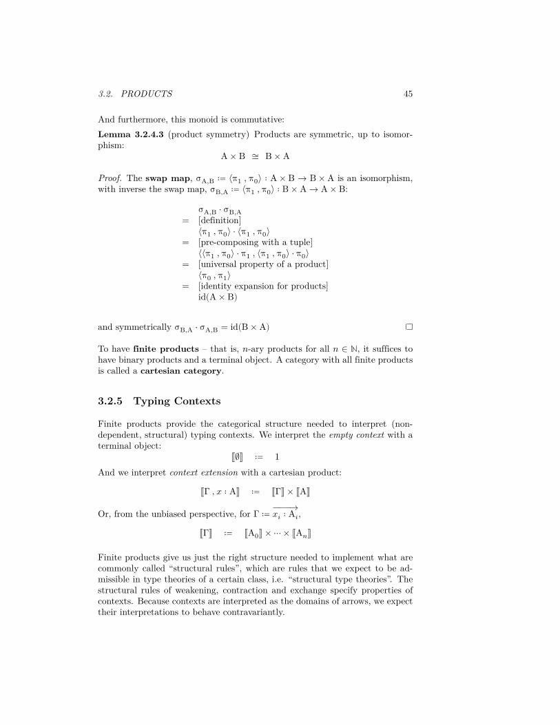
And furthermore, this monoid is commutative:Lemma 3.2.4.3 (product symmetry) Products are symmetric, up to isomor-phism:
A × B ≅ B × A
Proof. The swap map, σA,B ≔ ⟨π1 , π0⟩ ∶ A × B → B × A is an isomorphism,with inverse the swap map, σB,A ≔ ⟨π1 , π0⟩ ∶ B × A → A × B:
σA,B ⋅ σB,A= [definition]
⟨π1 , π0⟩ ⋅ ⟨π1 , π0⟩= [pre-composing with a tuple]
⟨⟨π1 , π0⟩ ⋅ π1 , ⟨π1 , π0⟩ ⋅ π0⟩= [universal property of a product]
⟨π0 , π1⟩= [identity expansion for products]
id(A × B)
and symmetrically σB,A ⋅ σA,B = id(B × A)
To have finite products – that is, 𝑛-ary products for all 𝑛 ∈ ℕ, it suffices tohave binary products and a terminal object. A category with all finite productsis called a cartesian category.
3.2.5 Typing Contexts
Finite products provide the categorical structure needed to interpret (non-dependent, structural) typing contexts. We interpret the empty context with aterminal object:
⟦∅⟧ ≔ 1And we interpret context extension with a cartesian product:
⟦Γ , 𝑥 ∶ A⟧ ≔ ⟦Γ⟧ × ⟦A⟧
Or, from the unbiased perspective, for Γ ≔ −−−→𝑥𝑖 ∶ A𝑖,
⟦Γ⟧ ≔ ⟦A0⟧ × ⋯ × ⟦A𝑛⟧
Finite products give us just the right structure needed to implement what arecommonly called “structural rules”, which are rules that we expect to be ad-missible in type theories of a certain class, i.e. “structural type theories”. Thestructural rules of weakening, contraction and exchange specify properties ofcontexts. Because contexts are interpreted as the domains of arrows, we expecttheir interpretations to behave contravariantly.

46 CHAPTER 3. UNIVERSAL CONSTRUCTIONS
The principle of context weakening says that a well-typed term remains so inthe presence of additional, unused assumptions:
Γ ⊢ M ∶ BΓ , 𝑥 ∶ A ⊢ M ∶ B 𝑐𝑤
Its categorical interpretation must be some means of constructing a memberof ⟦Γ⟧ × ⟦A⟧ → ⟦B⟧ from a member of ⟦Γ⟧ → ⟦B⟧. We can do this by simplypre-composing a projection, or equivalently, up to the unit isomorphism forproducts, the product of an identity arrow and a bang map:
⟦Γ⟧ × ⟦A⟧ ⟦Γ⟧ × 1 ⟦Γ⟧ ⟦B⟧id × ! ≅ ⟦M⟧
The principle of context contraction says that a well-typed term depending ontwo variables of the same type remains so when a single variable is substitutedfor both:
Γ , 𝑥 ∶ A , 𝑦 ∶ A ⊢ M ∶ BΓ , 𝑧 ∶ A ⊢ M[(𝑥 , 𝑦)↦(𝑧 , 𝑧)] ∶ B
𝑐𝑐
Its categorical interpretation must be some means of constructing a member of⟦Γ⟧ × ⟦A⟧ → ⟦B⟧ from a member of ⟦Γ⟧ × ⟦A⟧ × ⟦A⟧ → ⟦B⟧. We can do this bysimply pre-composing the product of an identity arrow and a diagonal map:
⟦Γ⟧ × ⟦A⟧ ⟦Γ⟧ × ⟦A⟧ × ⟦A⟧ ⟦B⟧id × ∆ ⟦M⟧
The principle of context exchange says that a well-typed term remains sounder a permution of its context:
Γ , 𝑦 ∶ B , 𝑥 ∶ A , Γ′ ⊢ M ∶ CΓ , 𝑥 ∶ A , 𝑦 ∶ B , Γ′ ⊢ M ∶ C
𝑐𝑥
Its categorical interpretation must be some means of constructing a member of⟦Γ⟧ × ⟦A⟧ × ⟦B⟧ × ⟦Γ′⟧ → ⟦C⟧ from a member of ⟦Γ⟧ × ⟦B⟧ × ⟦A⟧ × ⟦Γ′⟧ → ⟦C⟧.We can do this by simply pre-composing the product of identity arrows and aswap map:
⟦Γ⟧ × ⟦A⟧ × ⟦B⟧ × ⟦Γ′⟧ ⟦Γ⟧ × ⟦B⟧ × ⟦A⟧ × ⟦Γ′⟧ ⟦C⟧id × σ × id ⟦M⟧
So a system that a type theorist might call “structural”, a category theoristwould call “cartesian”: it is one in which we may duplicate and discard (as wellas reorder) elements of the context. Note that by convention, in type theoryweakening and exchange are “silent”, in the sense that we don’t record them inthe term itself.

3.3. COPRODUCTS 47
Exercise 3.2.5.1 In structural type theories, the variable rule and substitutionrule of baby type theory have the following genrealizations:
Γ , 𝑥 ∶ A ⊢ 𝑥 ∶ A 𝑣𝑎𝑟and
Γ ⊢ M ∶ B Γ , 𝑦 ∶ B ⊢ N ∶ CΓ ⊢ N[𝑦↦M] ∶ C 𝑠𝑢𝑏
Why are these generalizations sound in a setting where contexts are interpretedas finite products?
3.3 Coproducts
A coproduct is the dual construction to a product. Categorically, that is allthere is to say about the matter. But because of the asymmetry inherent intype theory – where inferences have a collection of assumptions, yet a singleconclusion – we will have to say a bit more when it comes to our categoricalsemantics for type theory.
First, we record for convenience, but without further comment, the duals of ourmain results about products. If you’re new to this, it would be an excellentexercise first to go back and see why these are the respective dual theorems,and then to prove each one explicitly – that is, by actually going through theargument, rather than by just saying, “by duality, Qed”.
3.3.1 Coproducts of Objects
Definition 3.3.1.1 (coproduct of objects) In any category, a coproduct ofobjects A and B is a cospan on A and B,
A𝑞0⟶ Q
𝑞1⟵ B
with the property that for any cospan on A and B,
A𝑥0⟶ X
𝑥1⟵ B
there is a unique map 𝑠 ∶ Q → X such that 𝑞0 ⋅ 𝑠 = 𝑥0 and 𝑞1 ⋅ 𝑠 = 𝑥1:
A Q B
X
𝑞0 𝑞1
𝑥0 𝑥1𝑠

48 CHAPTER 3. UNIVERSAL CONSTRUCTIONS
We call A and B the cases of the coproduct, 𝑞0 and 𝑞1 its insertions and 𝑠 thecotuple of 𝑥0 and 𝑥1, and write it as “[𝑥0 , 𝑥1]”.Probing a coproduct with itself by choosing X ≔ Q and (𝑥0 , 𝑥1) ≔ (𝑞0 , 𝑞1), welearn:Lemma 3.3.1.2 (identity expansion for coproducts) If Q is a coproduct of Aand B with insertions 𝑞0 and 𝑞1, then [𝑞0 , 𝑞1] = id(Q).And being characterized by a universal property, we expect:Lemma 3.3.1.3 (uniqueness of coproducts) When they exist, coproducts ofobjects are unique up to a unique insertion-preserving isomorphism.
We write “A + B” to refer to an arbitrary coproduct of A and B, When thecoproduct in question is clear from context, we refer to the two case insertionsgenerically as “ι0” and “ι1”.
In the category Set, the disjoint union of two sets is their coproduct. In Cat,there is something similar: ℂ + 𝔻 is the category whose collection of objectsis the disjoint union of those of ℂ and 𝔻 and whose homs between pairs of ℂ-objects is the same as in ℂ, and likewise for 𝔻, but where the “mixed” homs areempty.Definition 3.3.1.4 (codiagonal map) For every object A, the universal propertyof the coproduct gives a canonical codiagonal map, which forgets about casedistinction:
∇(A) ≔ [id(A) , id(A)] ∶ A + A → A
A A + A A
A
ι0 ι1
id id∇
Lemma 3.3.1.5 (post-composing with a cotuple) For a coproduct A + B, acotuple [𝑓 , 𝑔] ∶ A + B → X and an arrow 𝑗 ∶ X → Y,
[𝑓 , 𝑔] ⋅ 𝑗 = [𝑓 ⋅ 𝑗 , 𝑔 ⋅ 𝑗] ∶ A + B → Y
A A + B B
X
Y
ι0 ι1
𝑓 𝑔[𝑓 , 𝑔]
𝑗𝑓 ⋅ 𝑗 𝑔 ⋅ 𝑗

3.3. COPRODUCTS 49
3.3.2 Coproduct Functors
Definition 3.3.2.1 (coproduct of arrows) Given a pair of arrows 𝑓 ∶ A → Xand 𝑔 ∶ B → Y, and coproducts A + B and X + Y, we define the coproduct ofarrows 𝑓 + 𝑔 ∶ A + B → X + Y by:
𝑓 + 𝑔 ∶ A + B → X + Y𝑓 + 𝑔 ≔ [𝑓 ⋅ ι0 , 𝑔 ⋅ ι1]
By the universal property of the coproduct A + B, the arrow 𝑓 + 𝑔 is the uniquemorphism making the two squares commute:
A A + B B
X X + Y Yι0 ι1
ι0 ι1
𝑓 𝑔𝑓 + 𝑔
This allows us to characterize the coproduct as a bifunctor:Lemma 3.3.2.2 (functoriality of coproducts) If a category ℂ has coproductsfor each pair of objects, then the given definition of coproducts for arrows yieldsa functor,
– + – ∶ ℂ × ℂ → ℂcalled the coproduct functor.Lemma 3.3.2.3 (pre-composing a coproduct of arrows) For arrows 𝑓0 + 𝑓1 ∶A0 + A1 → B0 + B1 and [𝑔0 , 𝑔1] ∶ B0 + B1 → X,
(𝑓0 + 𝑓1) ⋅ [𝑔0 , 𝑔1] = [𝑓0 ⋅ 𝑔0 , 𝑓1 ⋅ 𝑔1]
A0 A0 + A1 A1
B0 B0 + B1 B1
X
ι0 ι1
ι0 ι1
𝑓0 𝑓1𝑓0 + 𝑓1
𝑔0 𝑔1[𝑔0 , 𝑔1]
Corollary 3.3.2.4 (cotuple factorization) A cotuple [𝑓 , 𝑔] ∶ A + B → X factorsthrough the codiagonal as,
[𝑓 , 𝑔] = (𝑓 + 𝑔) ⋅ ∇(X)

50 CHAPTER 3. UNIVERSAL CONSTRUCTIONS
A A + B B
X X + X X
X
ι0 ι1
ι0 ι1
𝑓 𝑔𝑓 + 𝑔
id id∇
3.3.3 Sum Types
The coproduct universal construction provides a possible categorical interpre-tation of sum types,
⟦A + B⟧ ≔ ⟦A⟧ + ⟦B⟧The introduction rules for sums,
Γ ⊢ M ∶ AΓ ⊢ inl(M) ∶ A + B
++0Γ ⊢ N ∶ B
Γ ⊢ inr(N) ∶ A + B++1
are then interpreted by the case insertions:
⟦inl(M)⟧ ≔ ⟦M⟧ ⋅ ι0 and ⟦inr(N)⟧ ≔ ⟦N⟧ ⋅ ι1In the restricted setting where contexts are singletons, the elimination rule forsums,
𝑥 ∶ A ⊢ P ∶ C 𝑦 ∶ B ⊢ Q ∶ C𝑧 ∶ A + B ⊢ case†(𝑥 . P ; 𝑦 . Q) ∶ C +−†
is then interpreted by the cotuple:
⟦case†(𝑥 . P ; 𝑦 . Q)⟧ ≔ [⟦P⟧ , ⟦Q⟧]
3.3.4 Distributive Categories
In order to interpret the full rule for sum elimination, which allows for an arbi-trary ambient context:
Γ , 𝑥 ∶ A ⊢ P ∶ C Γ , 𝑦 ∶ B ⊢ Q ∶ CΓ , 𝑧 ∶ A + B ⊢ case(𝑥 . P ; 𝑦 . Q)(𝑧) ∶ C +−
we need a categorical setting in which the distributive law holds:
𝑑𝑖𝑠𝑡 ∶ X × (A + B) ≅ (X × A) + (X × B)

3.3. COPRODUCTS 51
since, in this setting we could define
⟦case⟧ ≔ 𝑑𝑖𝑠𝑡 ⋅ [– , –]
orX × (A + B)
X × A (X × A) + (X × B) X × B
C
𝑑𝑖𝑠𝑡 ≅𝑞0 𝑞1
𝑓 𝑔[𝑓 , 𝑔]
Likewise, in order to interpret the full rule for void elimination, which also allowsfor an arbitrary ambient context:
Γ , 𝑧 ∶ ⊥ ⊢ abort(𝑧) ∶ A ⊥−
we need a categorical setting in which the absorption law holds:
𝑎𝑏𝑠 ∶ X × 0 ≅ 0
since, in this setting we could define
⟦abort⟧ ≔ 𝑎𝑏𝑠 ⋅ ¡
orX × 0
0
C
𝑎𝑏𝑠 ≅
¡
By duality with finite products, an initial object represents a nullary coprod-uct. So we can think of the absorption law as a nullary version on the distribu-tive law in the sense that in the latter the product distributes over the two casesof the coproduct, while in the former it distributes over the zero cases of theinitial object.
For the distributive law to hold we merely require the existence of some natural2isomorphism X × (A + B) → (X × A) + (X × B). It is a non-trivial theorem3
2We haven’t met naturality yet, but we soon will. It requires that the isomorphism we seekshould be “generic” in X, A and B.
3http://arxiv.org/abs/0912.2126
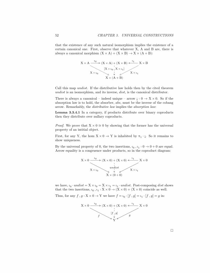
52 CHAPTER 3. UNIVERSAL CONSTRUCTIONS
that the existence of any such natural isomorphism implies the existence of acertain canonical one. First, observe that whatever X, A and B are, there isalways a canonical morphism (X × A) + (X × B) → X × (A + B):
X × A (X × A) + (X × B) X × B
X × (A + B)
ι0 ι1
X × ι0 X × ι1
[X × ι0 , X × ι1]
Call this map 𝑢𝑛𝑑𝑖𝑠𝑡. If the distributive law holds then by the cited theorem𝑢𝑛𝑑𝑖𝑠𝑡 is an isomorphism, and its inverse, 𝑑𝑖𝑠𝑡, is the canonical distributor.
There is always a canonical – indeed unique – arrow ¡ ∶ 0 → X × 0. So if theabsorption law is to hold, the absorber, 𝑎𝑏𝑠, must be the inverse of the cobangarrow. Remarkably, the distributive law implies the absorption law:Lemma 3.3.4.1 In a category, if products distribute over binary coproductsthen they distribute over nullary coproducts.
Proof. We prove that X × 0 ≅ 0 by showing that the former has the universalproperty of an intitial object.
First, for any Y, the hom X × 0 → Y is inhabited by π1 ⋅ ¡. So it remains toshow uniqueness.
By the universal property of 0, the two insertions, ι0 , ι1 ∶ 0 → 0 + 0 are equal.Arrow equality is a congruence under products, so in the coproduct diagram:
X × 0 (X × 0) + (X × 0) X × 0
X × (0 + 0)
ι0 ι1
X × ι0 X × ι1𝑢𝑛𝑑𝑖𝑠𝑡
we have, ι0 ⋅ 𝑢𝑛𝑑𝑖𝑠𝑡 = X × ι0 = X × ι1 = ι1 ⋅ 𝑢𝑛𝑑𝑖𝑠𝑡. Post-composing 𝑑𝑖𝑠𝑡 showsthat the two insertions, ι0 , ι1 ∶ X × 0 → (X × 0) + (X × 0) coincide as well.
Thus, for any 𝑓 , 𝑔 ∶ X × 0 → Y we have 𝑓 = ι0 ⋅ [𝑓 , 𝑔] = ι1 ⋅ [𝑓 , 𝑔] = 𝑔 in:
X × 0 (X × 0) + (X × 0) X × 0
Y
ι0 ι1
𝑓 𝑔[𝑓 , 𝑔]

3.4. EXPONENTIALS 53
A category with finite products and coproducts in which the distributive lawholds is called a distributive category. Furthermore, the presence of thenext universal construction we meet is sufficient to ensure that a category isdistributive.
3.4 Exponentials
As functional programmers, we are familiar with the idea of function currying,that is, of viewing a function of two arguments as a higher-order function thattakes the first argument and returns a new function, which, when provided thesecond argument, computes the same result as the original function when givenboth arguments at once. Once we get used to working with high-order functions,we wonder how we ever managed to program any other way.
3.4.1 Exponentials of Objects
Exponential objects are the categorical analogue of set-theoretic function space,allowing us to characterize function currying and λ-abstraction.Definition 3.4.1.1 (exponential object) In a category with binary products,an exponential of objects A and B is an object E together with an arrowε ∶ E × A → B with the property that for any object X and arrow 𝑓 ∶ X × A → Bthere is a unique arrow λ(𝑓) ∶ X → E such that λ(𝑓) × A ⋅ ε = 𝑓 :
X E
X × A B
E × A
ε
𝑓
λ(𝑓)
λ(𝑓) × A
We call ε the evaluation map of the exponential, and λ(𝑓) the exponentialtranspose or “curry” of 𝑓 .
Notice that the “such that” clause of the definition lets us recover 𝑓 from λ(𝑓):just take the product with id(A) and compose with ε. This is just “uncurrying”to functional programmers. If this isn’t clear to you, go back to the definitionsof product and coproduct and see how the same principle allows us to recover 𝑓and 𝑔 from ⟨𝑓 , 𝑔⟩ and from [𝑓 , 𝑔], respectively.
Let’s see what we learn from probing an exponential with itself by choosingX ≔ E and 𝑓 ≔ ε.

54 CHAPTER 3. UNIVERSAL CONSTRUCTIONS
Lemma 3.4.1.2 (identity expansion for exponentials) If E is an exponential ofA and B then λ(ε) = id(E).
Proof. By assumption, λ(ε) is the unique map in the hom set E → E with theproperty that λ(ε) × A ⋅ ε = ε:
E E
E × A B
E × A
ε
ε
λ(ε)
λ(ε) × A
By the left unit law of composition, id(E × A) ⋅ ε = ε, and by the definition ofa product of arrows, id(E × A) = id(E) × id(A). Since id(E) has the desiredproperty, the result follows from uniqueness.
To summarize:
• currying the evaluation map yields the identity on the exponential, and
• uncurrying the identity on the exponential yields the evaluation map.
Because exponentials are structures characterized by a universal property, weexpect them to be unique up to a unique structure-preserving isomorphism.This should be familiar by now.Lemma 3.4.1.3 (uniqueness of expoentials) When they exist, exponentials areunique up to a unique evaluation-preserving isomorphism.
Proof. Suppose that (E , ε , λ) and (E′ , ε′ , λ′) are both exponentials of A andB. By setting X ≔ E′ and 𝑓 ≔ ε′ in the universal property of E, we have:
E′ E
E′ × A B
E × A
ε
ε′
λ(ε′)
λ(ε′) × A
That is, λ(ε′) × A ⋅ ε = ε′. Symmetrically, by the universal property of E′, wehave λ′(ε) × A ⋅ ε′ = ε.

3.4. EXPONENTIALS 55
We want to show that λ′(ε) ⋅ λ(ε′) ∶ E → E is the identity map. We do so byuncurrying it:
(λ′(𝑒) ⋅ λ(ε′)) × id(A) ⋅ ε= [product functor]
λ′(𝑒) × id(A) ⋅ λ(ε′) × id(A) ⋅ ε= [universal property of E]
λ′(𝑒) × id(A) ⋅ ε′
= [universal property of E′]ε
So by identity expansion for exponentials, λ′(ε) ⋅ λ(ε′) = id(E).
E E′ E
E × A E′ × A B
E × A
ε
ε′
λ(ε′)
λ(ε′) × A
λ′(ε)
λ′(ε) × A
(λ′(ε) ⋅ λ(ε′)) × A
ε
id
Similarly, we have λ(ε′) ⋅ λ′(ε) = id(E′).So λ′(ε) ∶ E → E′ is an isomorphism. By the universal property of E′, it is theonly one that respects the evaluation ε′.
Because exponentials are determined as uniquely as is possible by a behavioralcharacterization, we write “A⊃B” to refer to an arbitrary exponential of A andB. The notation “BA” is also common.Definition 3.4.1.4 (pairing map) For every object A, the universal property ofthe exponential gives a canonical pairing map, which is a higher-order functionthat pairs an argument with a given parameter:
η(X) ≔ λ(id(X × A)) ∶ X → A ⊃ (X × A)
X A ⊃ (X × A)
X × A X × A
(A ⊃ (X × A)) × A
ε
id
η
η × A

56 CHAPTER 3. UNIVERSAL CONSTRUCTIONS
Exercise 3.4.1.5 (pre-composing with a curry) Use the diagram and the uni-versal property of an exponential object to prove the following:
For an exponential A ⊃ B, an arrow 𝑓 ∶ X × A → B and an arrow 𝑖 ∶ Y → X,
𝑖 ⋅ λ𝑓 = λ(𝑖 × A ⋅ 𝑓) ∶ Y → A ⊃ B
Y X A ⊃ B
Y × A X × A B
(A ⊃ B) × A
ε
𝑓
λ(𝑓)
λ(𝑓) × A
𝑖
𝑖 × A
(𝑖 ⋅ λ(𝑓)) × A
Having products and exponents lets a category talk about its own hom collec-tions, indeed exponential objects are sometimes called “internal homs”.
Given any arrow 𝑓 ∶ A → B, we can precompose it with the isomorphism1 × A → A from lemma 3.2.4.2 to obtain an arrow 𝑓 ′ ∶ 1 × A → B. We canthen curry this arrow to obtain an arrow ⌜𝑓⌝ ≔ λ(𝑓 ′) ∶ 1 → A ⊃ B, yielding aglobal element of the exponential called the name of 𝑓 .
For any object A, we always have the identity arrow id(A), and hence a globalelement ⌜id(A)⌝ ∶ 1 → A ⊃ A, the internal identity.
Given any objects A , B , C, we can form the composite:
((A ⊃ B) × (B ⊃ C)) × A
((B ⊃ C) × (A ⊃ B)) × A
(B ⊃ C) × ((A ⊃ B) × A)
(B ⊃ C) × B)
C
σ × A
α
(B ⊃ C) × ε
ε
where σ is the product symmetry isomorphism (lemma 3.2.4.3), α is the productassociativity isomorphism (lemma 3.2.4.1), and the εs are the respective eval-uation maps. Currying this map gives a map κ ∶ (A ⊃ B) × (B ⊃ C) → A ⊃ C,
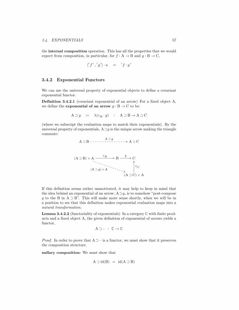
3.4. EXPONENTIALS 57
the internal composition operation. This has all the properties that we wouldexpect from composition, in particular, for 𝑓 ∶ A → B and 𝑔 ∶ B → C,
⟨⌜𝑓⌝ , ⌜𝑔⌝⟩ ⋅ κ = ⌜𝑓 ⋅ 𝑔⌝
3.4.2 Exponential Functors
We can use the universal property of exponential objects to define a covariantexponential functor.Definition 3.4.2.1 (covariant exponential of an arrow) For a fixed object A,we define the exponential of an arrow 𝑔 ∶ B → C to be:
A ⊃ 𝑔 ≔ λ(εB ⋅ 𝑔) ∶ A ⊃ B → A ⊃ C
(where we subscript the evaluation maps to match their exponentials). By theuniversal property of exponentials, A⊃𝑔 is the unique arrow making the trianglecommute:
A ⊃ B A ⊃ C
(A ⊃ B) × A B C
(A ⊃ C) × A
εC
εB 𝑔
A ⊃ 𝑔
(A ⊃ 𝑔) × A
If this definition seems rather unmotivated, it may help to keep in mind thatthe idea behind an exponential of an arrow, A⊃𝑔, is to somehow “post-compose𝑔 to the B in A ⊃ B”. This will make more sense shortly, when we will be ina position to see that this definition makes exponential evaluation maps into anatural transformation.Lemma 3.4.2.2 (functoriality of exponentials) In a category ℂ with finite prod-ucts and a fixed object A, the given definition of exponential of arrows yields afunctor,
A ⊃ – ∶ ℂ → ℂ
Proof. In order to prove that A ⊃ – is a functor, we must show that it preservesthe composition structure.
nullary composition: We must show that
A ⊃ id(B) = id(A ⊃ B)

58 CHAPTER 3. UNIVERSAL CONSTRUCTIONS
A ⊃ id(B)= [definition of A ⊃ – on arrows]
λ(εB ⋅ id(B))= [composition unit law]
λ(εB)= [identity expansion for exponentials]
id(A ⊃ B)
binary composition: We must show that
A ⊃ (𝑔 ⋅ ℎ) = A ⊃ 𝑔 ⋅ A ⊃ ℎ
In the diagram,
A ⊃ B A ⊃ C A ⊃ D
B C D
(A ⊃ B) × A (A ⊃ C) × A (A ⊃ D) × A
εB εC εD
𝑔 ℎ
A ⊃ 𝑔 A ⊃ ℎ
A ⊃ (𝑔 ⋅ ℎ)
(A ⊃ 𝑔) × A (A ⊃ ℎ) × A
𝑔 ⋅ ℎ
(A ⊃ (𝑔 ⋅ ℎ)) × A
(I) (II)
the outer square commutes by the definition of A ⊃ (𝑔 ⋅ ℎ) and the innersquares (I) and (II) commute by the definitions of A ⊃ 𝑔 and A ⊃ ℎ,respectively. By the functoriality of the cartesian product,
(A ⊃ 𝑔) × A ⋅ (A ⊃ ℎ) × A = (A ⊃ 𝑔 ⋅ A ⊃ ℎ) × A
By pasting squares (I) and (II), we see that:
εB ⋅ (𝑔 ⋅ ℎ) = (A ⊃ 𝑔) × A ⋅ (A ⊃ ℎ) × A ⋅ εD
The result follows by the uniqueness clause of the universal property ofexponentials.

3.5. CARTESIAN CLOSED CATEGORIES 59
3.4.3 Function Types
The exponential universal construction provides the categorical interpretationof function types,
⟦A → B⟧ ≔ ⟦A⟧ ⊃ ⟦B⟧
The introduction rule,
Γ , 𝑥 ∶ A ⊢ M ∶ BΓ ⊢ λ𝑥 . M ∶ A → B → +
is interpreted by currying:
⟦λ𝑥 . M⟧ ≔ λ(⟦M⟧)
and the elimination rule,
Γ ⊢ P ∶ A ⊃ B Γ ⊢ N ∶ AΓ ⊢ P N ∶ B → −
is interpreted by the evaluation map:
⟦P N⟧ ≔ ⟨⟦P⟧ , ⟦N⟧⟩ ⋅ ε
3.5 Cartesian Closed Categories
A category having all finite products (i.e. a terminal object and binary prod-ucts), as well as all exponentials, is known as a cartesian closed category. Acategory that additionally has all finite coproducts (i.e. an initial object andbinary coproducts) is called bicartesian closed.
It turns out that every bicartesian closed category is distributive. We don’t havetime to give a full explanation of why this is the case, but the short version isthat it can be seen using the Yoneda principle, which says essentially that forgiven objects X , Y ∶ ℂ, if for all objects Z, we have ℂ (X → Z) ≅ ℂ (Y → Z)in Set then X ≅ Y in ℂ. You should think of this as generalizing the followingfamiliar fact about preordered sets:
(∀Z . X ≤ Z ⟺ Y ≤ Z) implies X ≅ Y

60 CHAPTER 3. UNIVERSAL CONSTRUCTIONS
Using this principle, the distributive law follow from:
ℂ (X × (A + B) → Z)≅ [product symmetry]
ℂ ((A + B) × X → Z)≅ [currying]
ℂ (A + B → X ⊃ Z)≅ [uncotupling]
ℂ (A → X ⊃ Z) × ℂ (B → X ⊃ Z)≅ [uncurrying]
ℂ (A × X → Z) × ℂ (B × X → Z)≅ [product symmetry]
ℂ (X × A → Z) × ℂ (X × B → Z)≅ [cotupling]
ℂ ((X × A) + (X × B) → Z)

Chapter 4
Two Dimensional Structure
We have deliberately presented the universal constructions of a bicartesianclosed category in such a way as to highlight the parallels between them. Thereader may be wondering whether there is some more general construction lurk-ing in the wings, in terms of which terminal and initial objects, products, co-products and exponentials can all be described. This is indeed the case: themystery construction is called an “adjunction”. But in order to describe it wewill need to first understand some 2-dimensional category theory.
4.1 Naturality
Naturality is the carrier of the two-dimensional structure of categories of cate-gories. It imposes a sort of comprehension or uniformity principle that allows usto interpret a family of features within a particular category as a single featurein the ambient category of categories.
4.1.1 Natural Transformations
Definition 4.1.1.1 (natural transformation) For parallel functors, F , G ∶ ℂ →𝔻, a natural transformation φ from F to G is a functor φ ∶ ℂ → 𝔻→ (where𝔻→ is the arrow category of 𝔻) such that:
φ ⋅ dom = F and φ ⋅ cod = G
Explicitly, this means that,
• for each object A ∶ ℂ there is an arrow,
φ(A) ∶ 𝔻 (F(A) → G(A))
61

62 CHAPTER 4. TWO DIMENSIONAL STRUCTURE
called the component of φ at A, and
• for each arrow 𝑓 ∶ ℂ (A → B) there is a commuting square,
F(𝑓) ⋅ φ(B) = φ(A) ⋅ G(𝑓)
called the naturality square for φ at 𝑓 :
A B F(A) F(B)
G(A) G(B)
𝑓 F(𝑓)
G(𝑓)
ϕ(A) ϕ(B)
ℂ ∶ 𝔻 ∶
One way to think about this is that a functor “projects” an image of its domaincategory into its codomain category. In this sense, a functor acts as a lens,which may “distort” the structure of the source category by identifying distinctobjects or arrows. Under this interpretation, a component of a natural trans-formation acts as a “homotopy” between the images of an object cast by twoparallel functors, and a naturality square ensures that these object homotopiesare consistent with the images of arrows.
You may also think of the naturality square above as a “2-dimensional arrow”from the 1-dimensional arrow F(𝑓) to the 1-dimensional arrow G(𝑓), acting asthe “component” of φ at 𝑓 . But in an ordinary (1-dimensional) category, theonly “2-dimensional arrows” available are the trivial ones – i.e. equalities.
4.1.2 Functor Categories
Natural transformations provide a notion of arrows between parallel functors,turning a hom set into a hom category:Definition 4.1.2.1 (functor category) For categories ℂ and 𝔻, define the func-tor category, “Fun(ℂ , 𝔻)”, to have the following structure:
objects Fun(ℂ , 𝔻)0 ≔ functors from ℂ to 𝔻arrows Fun(ℂ , 𝔻) (F → G) ≔ natural transformations from F to Gidentities id(F)(A) ≔ id(F(A))
(A component of an identity natural transformation is an identity arrow.)
composition (φ ⋅ ψ)(A) ≔ φ(A) ⋅ ψ(A)(A component of a composite natural transformation is the compositionof the constituent components.)
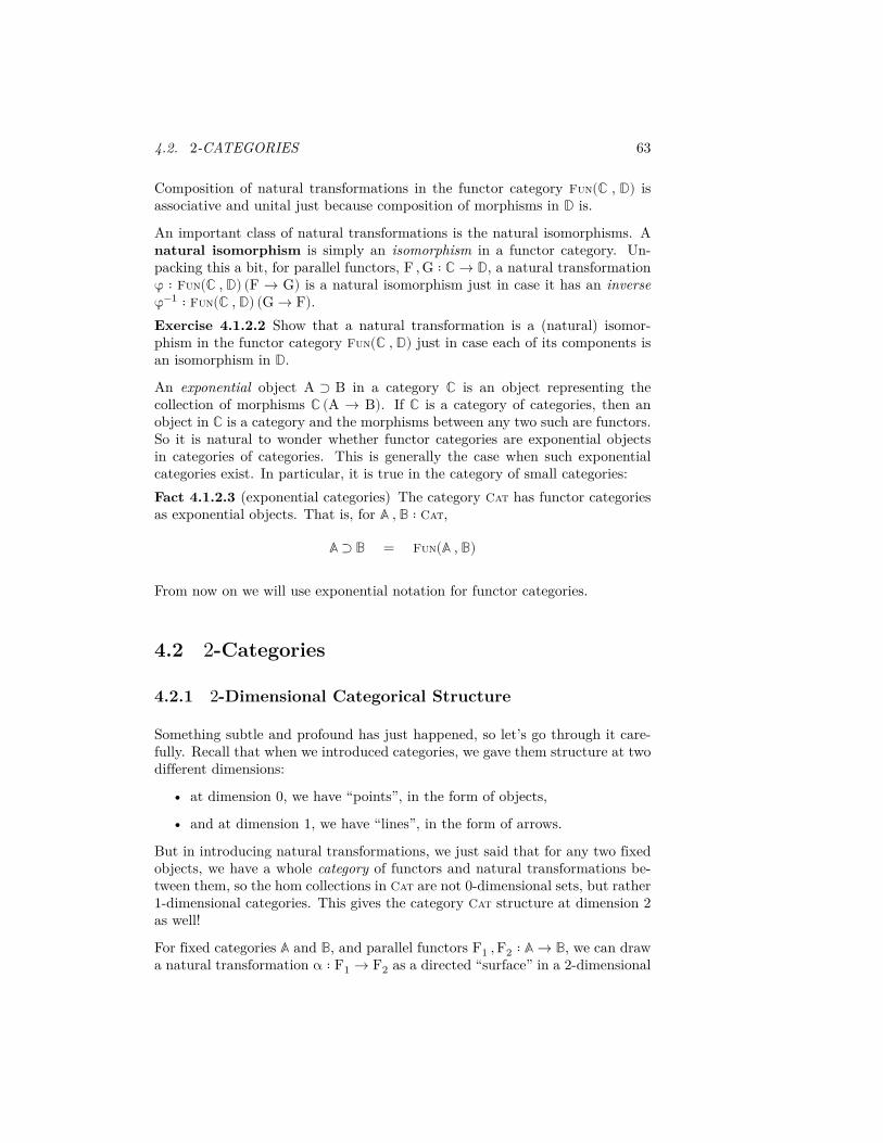
4.2. 2-CATEGORIES 63
Composition of natural transformations in the functor category Fun(ℂ , 𝔻) isassociative and unital just because composition of morphisms in 𝔻 is.
An important class of natural transformations is the natural isomorphisms. Anatural isomorphism is simply an isomorphism in a functor category. Un-packing this a bit, for parallel functors, F , G ∶ ℂ → 𝔻, a natural transformationφ ∶ Fun(ℂ , 𝔻) (F → G) is a natural isomorphism just in case it has an inverseφ−1 ∶ Fun(ℂ , 𝔻) (G → F).Exercise 4.1.2.2 Show that a natural transformation is a (natural) isomor-phism in the functor category Fun(ℂ , 𝔻) just in case each of its components isan isomorphism in 𝔻.
An exponential object A ⊃ B in a category ℂ is an object representing thecollection of morphisms ℂ (A → B). If ℂ is a category of categories, then anobject in ℂ is a category and the morphisms between any two such are functors.So it is natural to wonder whether functor categories are exponential objectsin categories of categories. This is generally the case when such exponentialcategories exist. In particular, it is true in the category of small categories:Fact 4.1.2.3 (exponential categories) The category Cat has functor categoriesas exponential objects. That is, for 𝔸 , 𝔹 ∶ Cat,
𝔸 ⊃ 𝔹 = Fun(𝔸 , 𝔹)
From now on we will use exponential notation for functor categories.
4.2 2-Categories
4.2.1 2-Dimensional Categorical Structure
Something subtle and profound has just happened, so let’s go through it care-fully. Recall that when we introduced categories, we gave them structure at twodifferent dimensions:
• at dimension 0, we have “points”, in the form of objects,
• and at dimension 1, we have “lines”, in the form of arrows.
But in introducing natural transformations, we just said that for any two fixedobjects, we have a whole category of functors and natural transformations be-tween them, so the hom collections in Cat are not 0-dimensional sets, but rather1-dimensional categories. This gives the category Cat structure at dimension 2as well!
For fixed categories 𝔸 and 𝔹, and parallel functors F1 , F2 ∶ 𝔸 → 𝔹, we can drawa natural transformation α ∶ F1 → F2 as a directed “surface” in a 2-dimensional
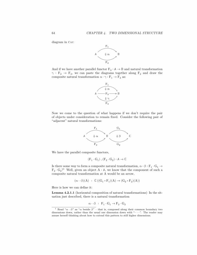
64 CHAPTER 4. TWO DIMENSIONAL STRUCTURE
diagram in Cat:
𝔸 𝔹
F1
F2
⇓ α
And if we have another parallel functor F3 ∶ 𝔸 → 𝔹 and natural transformationγ ∶ F2 → F3, we can paste the diagrams together along F2 and draw thecomposite natural transformation α ⋅ γ ∶ F1 → F3 as:
𝔸 𝔹
F1
F2
F3
⇓ α
⇓ γ
Now we come to the question of what happens if we don’t require the pairof objects under consideration to remain fixed. Consider the following pair of“adjacent” natural transformations:
𝔸 𝔹 ℂ
F1
F2
G1
G2
⇓ α ⇓ β
We have the parallel composite functors,
(F1 ⋅ G1) , (F2 ⋅ G2) ∶ 𝔸 → ℂ
Is there some way to form a composite natural transformation, α⋅⋅β ∶ F1 ⋅ G1 →F2 ⋅ G2?1 Well, given an object A ∶ 𝔸, we know that the component of such acomposite natural transformation at A would be an arrow,
(α ⋅ ⋅β)(A) ∶ ℂ ((G1 ∘ F1)(A) → (G2 ∘ F2)(A))
Here is how we can define it:Lemma 4.2.1.1 (horizontal composition of natural transformations) In the sit-uation just described, there is a natural transformation
α ⋅ ⋅β ∶ F1 ⋅ G1 → F2 ⋅ G21 Read “α ⋅ ⋅β” as “α beside β” – that is, composed along their common boundary two
dimensions down, rather than the usual one dimension down with “– ⋅ –”. The reader mayamuse herself thinking about how to extend this pattern to still higher dimensions.

4.2. 2-CATEGORIES 65
called the horizontal composition of α and β, with components,
(α ⋅ ⋅β)(A) ≔ G1(α(A)) ⋅ β(F2(A)) = β(F1(A)) ⋅ G2(α(A))
Proof. To see that the two composites are indeed equal consider the componentof α at A in 𝔹. This determines a naturality square for β at α(A) in ℂ:
F1(A) F2(A) G1(F1(A)) G1(F2(A))
G2(F1(A)) G2(F2(A))
α(A) G1(α(A))
G2(α(A))
β(F1(A)) β(F2(A))(α ⋅ ⋅β)(A)
𝔹 ∶ ℂ ∶
(4.1)establishing that the two expressions for the putative components of α ⋅ ⋅β areequal.
Now we must show that this definition of components respects arrows in 𝔸. Let𝑓 ∶ 𝔸 (A → B). Then in the diagram in ℂ,
G1(F1(A))
G1(F2(A))
G2(F1(A))
G2(F2(A))
G1(F1(B))
G1(F2(B))
G2(F1(B))
G2(F2(B))
β(F1(A))β(F1(B))
G1(F1(𝑓))
G2(F1(𝑓))β(F2(A))
β(F2(B))
G1(F2(𝑓))
G2(F2(𝑓))
G1(α(A))
G2(α(A))
G1(α(B))
G2(α(B))
• the left and right squares are the naturality squares for β at α(A) andα(B),
• the top and bottom squares are the G1 and G2 functor-images of thenaturality squares for α at 𝑓 ,
• and the back and front squares are the naturality squares for β at F1(𝑓)and F2(𝑓).
Pasting the top and front – or equivalently, the back and bottom – squaresestablishes the naturality of α ⋅ ⋅β at 𝑓 .
Remark 4.2.1.2 (connection to arrow categories) The construction in the pre-ceding proof should remind you of the double arrow category construction. This

66 CHAPTER 4. TWO DIMENSIONAL STRUCTURE
is because the arrow category ℂ→ is equivalent to the functor category 𝕀 ⊃ ℂ,where 𝕀 is the interval category.Exercise 4.2.1.3 Check that horizontal composition respects the compositionstructure of each functor category by pasting squares onto diagram 4.1.
Mercifully, we do not need to think about natural transformations in this cum-bersome, component-wise manner. After all, the whole point of the categoricalapproach is to allow us to reason behaviorally rather than structurally. Thecomponent-wise definition of natural transformations is reminiscent of Plato’sAllegory of the Cave: the component arrows and naturality squares in thecodomain category are mere one-dimensional shadows cast by the flesh-and-blood natural transformations, which are two-dimensional morphisms betweenparallel one-dimensional morphisms living in a 2-dimensional category of cate-gories. Let us turn our heads and stumble into the light.Definition 4.2.1.4 (2-category) A strict 2-dimensional globular category, or2-category, ℂ consists of the following data:
• A collection of 0-cells of ℂ.
• For each A , B ∶ ℂ, a hom category ℂ (A → B), whose objects are 1-cellsof ℂ and whose arrows are 2-cells of ℂ.
We write the composition of these arrows as “– ⋅–” and call it the “verticalcomposition of 2-cells”.
• For each A , B , C ∶ ℂ, a composition bifunctor:
κA,B,C ∶ ℂ (A → B) × ℂ (B → C) → ℂ (A → C)
We write its action on objects as “– ⋅ –” and call it the “composition of1-cells”. We write its action on arrows as “– ⋅ ⋅–” and call it the “horizontalcomposition of 2-cells”.
• For each A ∶ ℂ, an identity cell functor:
ηA ∶ 𝟙 → C (A → A)
We write the image of ⋆ as “id(A)” and call it the “identity 1-cell”. Wewrite the image if id(⋆) as “id2(A)” and call it the “double-identity 2-cell”.
This data is required to respect the following relations:

4.2. 2-CATEGORIES 67
composition unitality
𝟙 × ℂ (A → B) ℂ (A → A) × ℂ (A → B)
ℂ (A → B) ℂ (A → B)
ℂ (A → B) × 𝟙 ℂ (A → B) × ℂ (B → B)
λ−1
≅
ηA × id
κA,A,B
ρ−1
≅
id × ηB
κA,B,B
where λ and ρ are the product unit isomorphisms.
Explicitly, this means that in the situation:
A A B B
id(A)
id(A)
𝑓1
𝑓2
id(B)
id(B)
⇓ id2(A) ⇓ α ⇓ id2(B)
id(A) ⋅ 𝑓𝑖 = 𝑓𝑖 = 𝑓𝑖 ⋅ id(B) and id2(A) ⋅ ⋅α = α = α ⋅ ⋅id2(B)
composition associativity
(ℂ (A → B) × ℂ (B → C)) × ℂ (C → D) ℂ (A → C) × ℂ (C → D)
ℂ (A → B) × ℂ (B → C) × ℂ (C → D) ℂ (A → D)
ℂ (A → B) × (ℂ (B → C) × ℂ (C → D)) ℂ (A → B) × ℂ (B → D)
α𝑙≅
κA,B,C × id
κA,C,D
α𝑟
≅
id × κB,C,D
κA,B,D
where the αs are the product associativity isomorphisms.
Explicitly, this means that in the situation:
A B C D
𝑓1
𝑓2
𝑔1
𝑔2
ℎ1
ℎ2
⇓ α ⇓ β ⇓ γ
(𝑓𝑖 ⋅ 𝑔𝑖) ⋅ ℎ𝑖 = 𝑓𝑖 ⋅ (𝑔𝑖 ⋅ ℎ𝑖) and (α ⋅ ⋅β) ⋅ ⋅γ = α ⋅ ⋅(β ⋅ ⋅γ)

68 CHAPTER 4. TWO DIMENSIONAL STRUCTURE
The definition may seem daunting, but the intuition is straightforward. Wewant to be able to compose 1-cells along their common 0-cell boundaries and 2-cells along both their common 1-cell boundaries and along their common 0-cellboundaries. Furthermore, we want every composable configuration of 2-cellsto have a unique composite. The last goal is accomplished by the compositionunitality and associativity laws, together with the requirement that compositionbe a bifunctor, which implies the following:
nullary composition In the situation,
A B C
𝑓
𝑓
𝑔
𝑔
⇓ id ⇓ id
id(𝑓) ⋅ ⋅id(𝑔) = id(𝑓 ⋅ 𝑔)
binary composition In the situation,
A B C
𝑓1
𝑓2
𝑓3
𝑔1
𝑔2
𝑔3
⇓ α
⇓ γ
⇓ β
⇓ δ
(α ⋅ γ) ⋅ ⋅(β ⋅ ⋅δ) = (α ⋅ ⋅β) ⋅ (γ ⋅ ⋅δ)This relation is known as the interchange law.
The category Cat with its categories, functors and natural transformations, isa 2-category. Its hom categories are the functor categories, and its horizontalcomposition of 2-cells is the horizontal composition of natural transformations.
4.2.2 String Diagrams
If we take the Poincaré (or graph) dual of the 2-dimensional diagrams we havebeen drawing, we obtain a very useful graphical language for 2-categories, calledstring diagrams. Specifically, we will use “planar progressive” string diagramsto represent configurations of 0-, 1-, and 2-cells.
In the graphical language of string diagrams,
0-cells are represented by regions in the plane,
1-cells are represented by lines or “strings” or “wires”, (in our convention)progressing from top to bottom,

4.2. 2-CATEGORIES 69
2-cells are represented by points, fattened up into “nodes” or “beads” withthe wires representing their domain 1-cells entering from above, and thoserepresenting their codomain 1-cells exiting from below.
identity 1-cells are represented by a dashed wire, or usually, not at all,
1-cell composition is represented by juxtaposing wires side-by-side, separatedby the region representing their common boundary,
identity 2-cells are represented by a dashed node, or usually, not at all,
2-cell vertical composition is represented by wiring the output sockets of thefirst node to the input sockets of the second,
2-cell horizontal composition is represented by juxtaposing nodes, togetherwith their respective wires, side-by-side,
As an example, the pasting diagram for the interchange law becomes the stringdiagram:
𝑓1
𝑓2
𝑓3
𝑔1
𝑔2
𝑔3
α β
γ δA B C
Typically, we omit labeling the regions as their identities can always be inferred.
The commuting of diagram 4.1 in the definition of horizontal composition ofnatural transformations represents the notion of naturality as independence,depicted in string diagrams by the property that two beads without an output-to-input connection between them may freely “slide” past one another alongtheir wires, and it makes no difference which is above or below the other.
F1
F2
G1
G2
α
β=
F1
F2
G1
G2
α β =F1
F2
G1
G2α
β
The idea of independence is the heart of naturality; the rest of its propertiescan be recovered from this.
There is a handy “trick” for transforming diagrams within a category into stringdiagrams using global elements. Notice that for any object A ∶ ℂ there is afunctor (which we typically overload with the same name) A ∶ 𝟙 → ℂ picking out
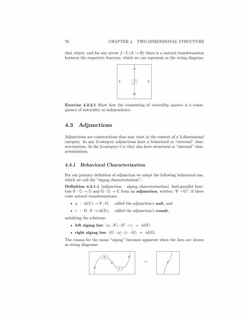
70 CHAPTER 4. TWO DIMENSIONAL STRUCTURE
that object, and for any arrow 𝑓 ∶ ℂ (A → B) there is a natural transformationbetween the respective functors, which we can represent as the string diagram:
A
B
𝑓𝟙 ℂ
Exercise 4.2.2.1 Show how the commuting of naturality squares is a conse-quence of naturality as independence.
4.3 Adjunctions
Adjunctions are constructions that may exist in the context of a 2-dimensionalcategory. In any 2-category adjunctions have a behavioral or “external” char-acterization. In the 2-category Cat they also have structural or “internal” char-acterizations.
4.3.1 Behavioral Characterization
For our primary definition of adjunction we adopt the following behavioral one,which we call the “zigzag characterization”:Definition 4.3.1.1 (adjunction – zigzag characterization) Anti-parallel func-tors F ∶ ℂ → 𝔻 and G ∶ 𝔻 → ℂ form an adjunction, written “F ⊣ G”, if thereexist natural transformations:
• η ∶ id(ℂ) → F ⋅ G, called the adjunction’s unit, and
• ε ∶ G ⋅ F → id(𝔻), called the adjunction’s counit,
satisfying the relations:
• left zigzag law: (η ⋅ ⋅F) ⋅ (F ⋅ ⋅ε) = id(F)• right zigzag law: (G ⋅ ⋅η) ⋅ (ε ⋅ ⋅G) = id(G)
The reason for the name “zigzag” becomes apparent when the laws are drawnas string diagrams:
FG
F
η
ε= F

4.3. ADJUNCTIONS 71
GF
G
η
ε= G
The chirality of the zigzag laws comes from the fact that when F ⊣ G, F iscalled left adjoint to G, and G is called right adjoint to F.
4.3.2 Structural Characterizations
Instead of thinking of an adjunction as a single structure living in the 2-categoryCat, we can think of it as a correlation between families of structures livingin two particular categories. This is like the component-wise presentation ofa natural transformation. One such characterization of an adjunction is thefollowing:Definition 4.3.2.1 (adjunction – natural bijection of hom sets charaterization)Anti-parallel functors F ∶ ℂ → 𝔻 and G ∶ 𝔻 → ℂ form an adjunction F ⊣ G iffor any A ∶ ℂ and B ∶ 𝔻 there is a natural bijection of hom sets:
ℂ (A → G(B))𝔻 (F(A) → B) θ
This characterization is internal or structural because, unlike the zigzag char-acterization, we look inside the categories ℂ and 𝔻. We will call the downwarddirection of such a bijection “–♯” and the upward direction “–♭”, so:
𝑓 ∶ ℂ (A → G(B)) –♯⟼ 𝑓 ♯ ∶ 𝔻(F(A) → B)and
𝑔 ∶ 𝔻 (F(A) → B) –♭⟼ 𝑔♭ ∶ ℂ(A → G(B))and
(𝑓 ♯)♭ = 𝑓 and (𝑔♭)♯ = 𝑔
We call the image of an arrow under this bijection its adjoint complement.
A bijection of hom sets is natural if it extends along its boundary by the relevantfunctors. In this case, that means that for any 𝑎 ∶ ℂ (A′ → A) and 𝑏 ∶ 𝔻 (B → B′)we have,
A′ A G(B) G(B′)
F(A′) F(A) B B′
𝑎
F(𝑎) 𝑏
G(𝑏)𝑓 = 𝑔♭
𝑔 = 𝑓♯
ℂ ∶
𝔻 ∶

72 CHAPTER 4. TWO DIMENSIONAL STRUCTURE
Technically, this is a natural isomorphism in the functor category (ℂ°×𝔻)⊃Setbetween ℂ (1– → G(2–)) and 𝔻 (F(1–) → 2–).We won’t prove the equivalence of the various characterizations of adjunctionsin this course, but the fact that the zigzag characterization implies the naturalbijection of hom sets characterization is easy to see using string diagrams.
Given an arrow 𝑓 ∶ ℂ (A → G(B)), the obvious way to construct an arrow𝑓 ♯ ∶ 𝔻(F(A) → B) out of the parts at hand is by defining,
𝑓 ♯ ≔ F(𝑓) ⋅ ε(B)
A
B G
𝑓–♯
⟼
A
BG
F𝑓
ε
Likewise, given an arrow 𝑔 ∶ 𝔻 (F(A) → B), the obvious way to construct anarrow 𝑔♭ ∶ ℂ(A → G(B)) is by defining,
𝑔♭ ≔ η(A) ⋅ G(𝑔)
A
B
F
𝑔–♭
⟼A
B
F
G𝑔
η
We can use the zigzag laws to show that –♯ and –♭ are inverse operations:
(𝑓 ♯)♭ =A
BG
FG
𝑓ε
η=
A
BG F
G
𝑓
ε
η =A
B G
𝑓
(𝑔♭)♯ =A
B
FG
F𝑔
ε
η=
A
B
F GF
𝑔ε
η=
A
B
F
𝑔
The naturality of the bijection in the domain and codomain coordinates is alsoobvious in the graphical language.

4.3. ADJUNCTIONS 73
• For naturality in the codomain coordinate, given 𝑏 ∶ 𝔻 (B → B′) we have:
𝑓 ♯⋅𝑏 =
A
B
B′
G
F𝑓
𝑏ε
=
A
B
B′
G
F𝑓
𝑏ε
= (𝑓⋅G(𝑏))♯
• For naturality in the domain coordinate, given 𝑎 ∶ ℂ (A′ → 𝑎) we have:
𝑎⋅𝑔♭ =
A′
A
B
F
G𝑔
𝑎η =
A′
A
B
F
G𝑔
𝑎η
= (F(𝑎)⋅𝑔)♭
Exercise 4.3.2.2 With 𝑓 , 𝑔, 𝑎 and 𝑏 as in the proof above, verify the following:
• (𝑔 ⋅ 𝑏)♭ = 𝑔♭ ⋅ G(𝑏)• (𝑎 ⋅ 𝑓)♯ = F(𝑎) ⋅ 𝑓 ♯
We can work out that the adjoint complements of components of the unit andcounit of an adjunction are identities, which are easily seen in string diagrams:
id(G(B)) = B G–♯
⟼ BG F
ε= ε(B)
id(F(A)) = A F–♭
⟼ AF G
η = η(A)
Two more structural characterizations of an adjunction – which are dual to oneanther – are given by the universal properties of its unit and counit.Definition 4.3.2.3 (adjunction – universal property of unit characterization)Anti-parallel functors F ∶ ℂ → 𝔻 and G ∶ 𝔻 → ℂ form and adjunction F ⊣ G ifthere is a natural transformation η ∶ id(ℂ) → F ⋅ G such that for any 𝑓 ∶ ℂ (A →

74 CHAPTER 4. TWO DIMENSIONAL STRUCTURE
G(B)) there is a unique 𝑔 ∶ 𝔻 (F(A) → B) such that η(A) ⋅ G(𝑔) = 𝑓 :
(G ∘ F)(A)
A G(B)
F(A) B
η(A)
𝑓
𝑔
G(𝑔)
ℂ ∶
𝔻 ∶
Definition 4.3.2.4 (adjunction – universal property of counit characterization)Anti-parallel functors F ∶ ℂ → 𝔻 and G ∶ 𝔻 → ℂ form and adjunction F ⊣ Gif there is a natural transformation ε ∶ G ⋅ F → id(𝔻) such that for any 𝑔 ∶𝔻 (F(A) → B) there is a unique 𝑓 ∶ ℂ (A → G(B)) such that F(𝑓) ⋅ ε(B) = 𝑔:
A G(B)
F(A) B
(F ∘ G)(B)
ε(B)
𝑔
𝑓
F(𝑓)
ℂ ∶
𝔻 ∶
Of course, 𝑔 = 𝑓 ♯ and 𝑓 = 𝑔♭. So the “internal picture” of an adjunction lookslike this:
(G ∘ F)(A)
A G(B)
F(A) B
(F ∘ G)(B)
η(A)
ε(B)
𝑓 = 𝑔♭
𝑔 = 𝑓♯
G(𝑓♯)
F(𝑔♭)
β𝑟 ⇑
⇓ β𝑙ℂ ∶
𝔻 ∶
The 2-cells labeled “β𝑙” and “β𝑟” are both equalities because ℂ and 𝔻 are justordinary (1-dimensional) categories so equality is the only possible kind of 2-cell.But it is convenient to give them a suggestive name and orientation.

4.3. ADJUNCTIONS 75
4.3.3 Conversion Relations
The universal property of the counit should immediately remind you of thedefinition of an exponential object. Indeed, for a fixed object A, we have endo-functors
– × A ∶ ℂ → ℂ and A ⊃ – ∶ ℂ → ℂand an adjunction
– × A ⊣ A ⊃ –The counit of this adjunction is the evaluation map and the unit is the pairingmap. The internal picture of this adjunction looks like this:
A ⊃ (X × A)
X A ⊃ B
X × A B
(A ⊃ B) × A
η(X)
ε(B)
λ(𝑓)
𝑓
A ⊃ 𝑓
λ(𝑓) × Aβ𝑟 ⇑
ℂ ∶
ℂ ∶
Recall our interpretations for the introduction and elimination rules for functiontypes interpreted as exponentials (section 3.4.3):
⟦λ𝑥 . M⟧ ≔ λ(⟦M⟧) and ⟦P N⟧ ≔ ⟨⟦P⟧ , ⟦N⟧⟩ ⋅ ε
where Γ , 𝑥 ∶ A ⊢ M ∶ B, Γ ⊢ N ∶ A, and Γ ⊢ P ∶ A → B. The universalproperty of exponentials is just the universal property of the counit of thisadjunction. Its commuting triangle β𝑟,
λ(𝑓) × A ⋅ ε(B) = 𝑓
expresses the β-equivalence relation for function type:
(λ𝑥 . M)N β≃ M[𝑥↦N]
as
⟦Γ⟧ ⟦Γ⟧ × ⟦A⟧ ⟦B⟧
(⟦A⟧ ⊃ ⟦B⟧) × ⟦A⟧
ε
⟦M⟧
λ⟦M⟧ × ⟦𝑥⟧
⟨id , ⟦N⟧⟩
⟨λ⟦M⟧ , ⟦N⟧⟩

76 CHAPTER 4. TWO DIMENSIONAL STRUCTURE
Furthermore, the bijection between the arrows 𝑓 and λ(𝑓) expresses the η-equivalence relation for function type:
Pη≃ λ𝑥 . P𝑥
as
⟦Γ⟧ ⟦A ⊃ B⟧
⟦Γ⟧ × ⟦A⟧ ⟦B⟧
(⟦A⟧ ⊃ ⟦B⟧) × ⟦A⟧
ε
⟦P 𝑥⟧
⟦P⟧
⟦P⟧ × ⟦𝑥⟧⏟⏟⏟⏟⏟⟨π0 ⋅⟦P⟧,π1⋅⟦𝑥⟧⟩
where ⟦P⟧ × ⟦𝑥⟧ = ⟨π0 ⋅ ⟦P⟧ , π1 ⋅ ⟦𝑥⟧⟩ by lemma 3.2.1.2 and exercise 3.2.2.3, andthe projections interpret context weakening, which is silent in the syntax of typetheory.
Indeed, the βη-conversion relations of all the simple types we have consideredhere can be characterized in this way due to the existence of adjunctions
– + – ⊣ ∆ ⊣ – × – and 0 ⊣ ! ⊣ 1
where ∆ and ! are respectively the diagonal and bang functors:
∆ℂ ⟶ ℂ × ℂA ⟼ (A , A)𝑓 ⟼ (𝑓 , 𝑓)
!ℂ ⟶ 𝟙A ⟼ ⋆𝑓 ⟼ id(⋆)
4.3.4 Context Distributivity Revisited
The context distributivity laws for the positively-presented types, the distribu-tive law and absorption law, are actually both instances of a more general resultabout cartesian closed categories and adjoint functors called Frobenius reci-procity.Proposition 4.3.4.1 (Frobenius reciprocity) For anti-parallel functors F ∶ ℂ →𝔻 and G ∶ 𝔻 → ℂ between cartesian closed categories, if there is an adjunctionF ⊣ G and the right adjoint G preserves exponentials then for objects A ∶ ℂ andX ∶ 𝔻,
X × F(A) ≅ F(G(X) × A)
The idea is that X is the interpretation of some ambient context and F is thefunctor determining some positively-presented type. Admittedly, the condition

4.3. ADJUNCTIONS 77
that G preserves exponentials seems unmotivated, but when you try to provethe result, you see that it is exactly what is needed to make it go through.
Proof. By the Yoneda principle, for an arbitrary Z ∶ 𝔻,
𝔻 (X × F(A) → Z)≅ [product symmetry]
𝔻 (F(A) × X → Z)≅ [currying]
𝔻 (F(A) → X ⊃ Z)≅ [adjoint complement –♭]
ℂ (A → G(X ⊃ Z))≅ [assumption that G preserves exponentials]
ℂ (A → G(X) ⊃ G(Z))≅ [uncurrying]
ℂ (A × G(X) → G(Z))≅ [adjoint complement –♯]
𝔻 (F(A × G(X)) → Z)≅ [product symmetry]
𝔻 (F(G(X) × A) → Z)
For example, in the case of the adjunction – + – ⊣ ∆, Frobenius reciprocity tellsus:
X × (+(A , B)) ≅ +(∆(X) × (A , B))or, in other words:
X × (A + B) ≅ (X × A) + (X × B)
which is the distributive law!
What is really going on here is that there is a natural isomorphism in the functorcategory (𝔻 × ℂ) ⊃ 𝔻,
1– × F(2–) ≅ F(G(1–) × 2–)