basic concepts of random matrix theory
TRANSCRIPT

Basic Concepts of Random Matrix Theory
Alexis J van Zyl
Thesis presented in partial fulfilment of the requirements for the degree of Master of Physics at the University of Stellenbosch.
Supervisor: Prof. F. G. Scholtz December 2005

2
Declaration I, the undersigned, hereby declare that the work contained in this thesis is my own original work and that I have not previously in its entirety or in part submitted it at any university for a degree. Signature: _____________________ Date:_____________________

Abstract It was Wigner that in the 1950’s first introduced the idea of modelling physical reality with an ensemble of random matrices while studying the energy levels of heavy atomic nuclei. Since then, the field of Random Matrix Theory has grown tremendously, with applications ranging from fluctuations on the economic markets to M-theory. It is the purpose of this thesis to discuss the basic concepts of Random Matrix Theory, using the ensembles of random matrices originally introduced by Wigner, the Gaussian ensembles, as a starting point. As Random Matrix Theory is classically concerned with the statistical properties of levels sequences, we start with a brief introduction to the statistical analysis of a level sequence before getting to the introduction of the Gaussian ensembles. With the ensembles defined, we move on to the statistical properties that they predict. In the light of these predictions, a few of the classical applications of Random Matrix Theory are discussed, and as an example of some of the important concepts, the Anderson model of localization is investigated in some detail. Opsomming Dit was in die 1950’s dat Wigner, besig om te werk in die veld van kern fisika, eerste was om voor te stel dat die fisiese wêreld gemodelleer kan word met behulp van ’n versameling willekeurig verkose matrikse. Sedert dien het die veld van Willekeurige Matriks Teorie geweldig gegroei, met toepassings in velde so uiteenlopend soos die finansiële markte en M-teorie. Dit is die doel van hierdie tesis om ’n breë oorsig te gee van die basiese konsepte van hierdie veld, met die oorspronklike matriks versamelings wat Wigner self voorgestel het, die Gaussiese versamelings, as vertrekpunt. Aangesien Willekeurige Matriks Teorie hoofsaaklik handel oor die statistiek van rye begin ons die tesis met ’n vlugtige oorsig van die statistiese analise van ’n ry getalle, voordat ons Wigner se matriks versamelings voorstel. Met dié versamelings gedefinieer, kyk ons dan na die ry-statistieke wat hulle voorspel, en gee dan voorbeelde van waar hierdie voorspellings in die praktyk suksesvol gevind is. As ’n gedetailleerde voorbeeld van die belangriker konsepte van Willekeurige Matriks Teorie, word die Anderson model van lokalisasie in sekere detail ondersoek.
3
Table of Contents
1 INTRODUCTION............................................................................................................................... 7
2 ANALYSIS OF A LEVEL SEQUENCE......................................................................................... 11
2.1 A SEQUENCE OF LEVELS ............................................................................................................. 11 2.2 LEVEL STATISTICS...................................................................................................................... 11
2.2.1 The Nearest neighbour spacing distribution......................................................................... 12 2.2.2 The two level correlation function ........................................................................................ 14 2.2.3 The number variance ............................................................................................................ 15 2.2.4 The 3∆ statistic .................................................................................................................... 15 2.2.5 Connection between the statistics ......................................................................................... 18
2.3 UNFOLDING A SEQUENCE ........................................................................................................... 18
3 ENSEMBLES OF RANDOM MATRICES.................................................................................... 21
3.1 MODELLING PHYSICAL REALITY WITH AN ENSEMBLE OF MATRICES........................................... 21 3.2 THE GAUSSIAN ORTHOGONAL ENSEMBLE ................................................................................. 22
3.2.1 The elements of a matrix in the GOE.................................................................................... 23 3.2.2 The joint probability density function................................................................................... 24 3.2.3 Physical considerations built into the GOE.......................................................................... 25
3.2.3.1 Symmetry................................................................................................................................... 26 3.2.3.2 Invariance under basis transformation ....................................................................................... 28 3.2.3.3 Size of the matrices and Block Diagonal form........................................................................... 31
3.2.4 A not so physical consideration and how it was fixed .......................................................... 33 3.2.4.1 Independence of matrix elements............................................................................................... 33 3.2.4.2 The Circular Ensembles ............................................................................................................. 33
3.3 THE GAUSSIAN UNITARY AND SYMPLECTIC ENSEMBLES ........................................................... 34 3.3.1 The Gaussian Unitary Ensemble .......................................................................................... 34 3.3.2 The Gaussian Symplectic Ensemble ..................................................................................... 36
3.4 MORE ENSEMBLES...................................................................................................................... 38 3.4.1 The Crossover between GOE and GUE ............................................................................... 38 3.4.2 More general ensembles ....................................................................................................... 40
3.5 SUMMARY.................................................................................................................................. 41 3.5.1 Why ensembles of random matrices?.................................................................................... 41 3.5.2 Considerations built into the Gaussian ensembles ............................................................... 42 3.5.3 How the considerations were built into the Gaussian ensembles ......................................... 43
4

3.5.4 A few practical notes ............................................................................................................ 44
4 LEVEL STATISTICS OF RANDOM MATRIX ENSEMBLES.................................................. 47
4.1 COMPARING THEORY AND EXPERIMENT ..................................................................................... 47 4.2 THE EIGENVALUE JOINT PROBABILITY DENSITY FUNCTION ........................................................ 48
4.2.1 A change of variables ........................................................................................................... 49 4.2.2 The eigenvalue j.p.d.f............................................................................................................ 51 4.2.3 The β parameter................................................................................................................. 53
4.3 THE COULOMB GAS ANALOGY ................................................................................................... 55 4.4 LEVEL STATISTICS OF THE GAUSSIAN ENSEMBLES ..................................................................... 58
4.4.1 The Density of States ............................................................................................................ 59 4.4.1.1 The large N limit ........................................................................................................................ 59 4.4.1.2 Dependence on size.................................................................................................................... 60 4.4.1.3 More than just Gaussian ensembles ........................................................................................... 62
4.4.2 The Nearest Neighbour Spacing distribution ....................................................................... 64 4.4.3 The two level correlation function ........................................................................................ 68 4.4.4 The number variance ............................................................................................................ 69 4.4.5 The 3∆ statistic .................................................................................................................... 71
4.5 SUMMARY.................................................................................................................................. 73
5 APPLICATIONS .............................................................................................................................. 77
5.1 LOCALIZATION........................................................................................................................... 77 5.1.1 The Anderson model in general ............................................................................................ 79 5.1.2 The Anderson model in two dimensions ............................................................................... 80 5.1.3 The 2D Anderson model in an external magnetic field......................................................... 82 5.1.4 Numerical experiments ......................................................................................................... 85
5.1.4.1 The density of states and the unfolding procedure ..................................................................... 86 5.1.4.2 Local statistics............................................................................................................................ 88
5.2 MORE APPLICATIONS................................................................................................................. 91 5.2.1 Nuclear Physics .................................................................................................................... 91 5.2.2 Quantum Chaos .................................................................................................................... 93 5.2.3 Acoustic resonances ............................................................................................................. 95
6 CLOSING REMARKS..................................................................................................................... 99
6.1 WHY DOES RMT WORK?............................................................................................................ 99 6.1.1 Universality .......................................................................................................................... 99
6.1.1.1 The Coulomb gas analogy revisited ......................................................................................... 100
5

6.1.1.2 Geometric Correlations ............................................................................................................ 102 6.1.2 Level repulsion ................................................................................................................... 102
6.2 CONCLUSION............................................................................................................................ 104
APPENDIX A ........................................................................................................................................... 106
APPENDIX B............................................................................................................................................ 107
APPENDIX C ........................................................................................................................................... 109
APPENDIX D ........................................................................................................................................... 111
REFERENCES ......................................................................................................................................... 112
6

1 Introduction
The study of matrices with random entries goes back as far as the 1920’s, where it was introduced by Wishard [1] while working in the field of mathematical statistics. It was not until the 1950’s however, that the thought of modelling physical reality with a set of specifically chosen random matrices emerged. In standard quantum mechanics, the Schrödinger equation, in principle, completely determines the dynamics of any system under inspection. Even though this famous equation may seem relatively simple at a glance, it quickly becomes very difficult to solve as the systems it is used to describe become more complicated. In fact, there are only a few very simple examples that can be solved exactly, and as the complexity of systems under inspection grows one soon has to resort to approximation. For large, multi-particle systems, such as heavy nuclei, the task of finding an exact solution, or even a good approximation thereof, is for all intents and purposes impossible. If one is to find any physical information of such a complex system at all, a different approach to the problem will have to be taken. It was in this context that Wigner [2] introduced the thought of modelling physical reality with a set of specifically chosen random matrices, and to better understand why and how he did this, let us take a look at a more specific example. In the scattering of low energy neutrons from medium and heavy nuclei, sharp resonances in absorption energy were observed, each of these resonances corresponding to a long lived semi-stable exited state of a “new” nucleus. These exited states happen when the incident neutron “gets stuck” in the target nucleus forming a new nucleus with one more neutron, sharing its kinetic energy between all the constituents of the original nucleus and thereby leaving it in an excited state. It then takes a while1 for a neutron to gather up enough energy again to get ejected from the nucleus, i.e. the newly formed nucleus to decay back to its original form; the ejected neutron’s momentum being uncorrelated with the incident one. The bombarded nuclei, however, only absorbed neutrons with specific energies, these energies corresponding to excitation energies of the newly formed nuclei. Figure 1 shows an example of absorption by thorium nuclei of incident neutrons as a function of their energy, each of the peaks corresponding to an excited state. 1 ‘A while’ here refers to a length of time much longer than the time it would take for a neutron to get kicked out of the back of the nucleus elastically due to the incident one hitting the front.
7

Figure 1: A slow neutron resonance cross section of thorium 232, taken from [3]. Each peak corresponds to a “semi stable” excited state. Even though the spacing of these resonances seem to be quite random, they are completely deterministic - reproducible.
Seeing as the nucleus of a thorium atom is quite complicated, it comes as no surprise that its energy spectrum, although obviously fixed, is rather hard to describe. If one did have the Hamiltonian of the system, one could in principle do this by calculating the energies and the states of the system by solving the Schrödinger equation
i iH E iψ ψ= (1.1)
where denotes the Hamiltonian, the H iE ’s the energy levels and the iψ ’s are the states of the system2. As just mentioned, solving this equation to find the energy spectrum of a complex system such as this is already virtually impossible. Unfortunately, the problem of finding the energy levels and states of such a system goes even deeper. It is not even possible to write down the Hamiltonian of such a complex system in the first place. Instead of trying to solve such a complicated system exactly, Wigner approached the problem from a statistical point of view. The idea he proposed is loosely as follows: instead of trying to find a specific Hamiltonian that describes the system in question exactly and then trying to solve the corresponding Schrödinger equation, one should rather consider the statistical properties of an large ensemble of Hamiltonians, all with the same general properties that the specific Hamiltonian would have had if it could be found. In principle, this specific Hamiltonian does lie somewhere in the ensemble, even though finding it is not possible. Instead, it is hoped, that for a well chosen ensemble
2 It is possible to write down the Schrödinger equation in both differential equation and matrix forms. In matrix form the Hamiltonian is square matrix, often of large, or even infinite dimension. It is with this form in mind that most of what follows has been written.
8

some general properties of the spectra of individual Hamiltonians in the ensemble, and therefore the specific Hamiltonian as well, are, on average, close to the these properties averaged over the whole of the ensemble. This may seem to be a strange way of approaching the problem, giving up hope of finding the levels and states of a system exactly, but it is an approach that is much the same as that of statistical mechanics. In [4], Freeman Dyson explains the similarities, and the necessary differences, between the approach of Random Matrix Theory and that of classical statistical mechanics: “In ordinary statistical mechanics a comparable renunciation of exact knowledge is made. By assuming all states of a very large ensemble to be equally probable, one obtains useful information about the over-all behaviour of a complex system, when the observation of the state of the system in all its detail is impossible. This type of statistical mechanics is clearly inadequate for the discussion of nuclear energy levels. We wish to make statements about the fine detail of the level structure, and such statements cannot be made in terms of an ensemble of states. What is here required is a new kind of statistical mechanics, in which we renounce exact knowledge not of the state of a system but of the nature of the system itself. We picture a complex nucleus as a “black box” in which a large number of particles are interacting according to unknown laws. The problem is then to define in a mathematically precise way an ensemble of systems in which all possible laws of interaction are equally probable.” Random Matrix Theory deals with defining ensembles of matrices, and finding from these ensembles average properties of spectra and states of their constituents, in an attempt to describe specific physical systems in a statistical manner. Even though, as Dyson said, this statistical approach renounces exact information regarding the detailed properties of a specific system, new properties regarding large systems can be found that can only be seen when looking at them statistically, much like properties such as temperature can only be seen by looking at very large systems in classical statistical mechanics. Random Matrix Theory (RMT) has proven to be an astonishingly successful “new kind of statistical mechanics”, which has over the years found a vast array of application not only in quantum mechanics, but also in the study of other complex systems ranging from sonic resonances in quartz crystal to the financial markets. Furthermore, it has even been applied in the study of systems that behave chaotically, even those with only a few
9

parameters, where a direct calculation of the evolution of the system from some initial state is impossible and one has to resort to a statistical description. It is clear, since the pioneering work of Wigner in the 1950’s, that RMT has become a very useful tool in the study of non-integrable systems, so much so that it has become a field of study in its own right. Since RMT is classically concerned with the description of sequences of levels, we shall diverge a bit from the main topic of this thesis in Chapter 2 for a brief introduction to the analysis of a level sequence. In Chapter 3 we shall discuss in more detail the classical ensembles of matrices introduced by Wigner, and the physical considerations that went into their construction. We shall also take a look at a few other ensembles that have been constructed in the literature, and place Wigner’s ensembles in the context of more general ensembles. In Chapter 4 we will give an overview of the basic statistical properties of level sequences derived from the ensembles introduced in Chapter 3. There is an interesting analogy, in this respect, between the distributions of these level sequences and a simple physical system of interacting particles trapped in a potential. This creates a very instructive intuitive picture of how energy levels of systems arrange themselves. This is closely related to the important concept in RMT called universality, and we conclude by discussing it in Chapter 6. Before we get there though, Chapter 5 will deal with the Anderson model of localisation as an extended example of some of the more important concepts of RMT discussed in the previous chapters, as well as a few other examples of where RMT has been applied with success. Much of this thesis is based on the review articles by Brody et al. [5], the Heidelberg group [6] and Beenakker [7], course notes of an introductory course in RMT by Eynhart [8], and, of course, the “canonical” book on Random Matrix Theory by Mehta [9]. Another important reference that should be mentioned is the reprint collection of the most influential papers in the early development of RMT, edited by Porter [10]. Throughout this thesis it should be clear out of context where special attention has been given to independently verify well known results. Figures, for instance, that have not been independently produced, have been indicated via references. Even though this thesis is essentially a literature study, some original work has been done (to our knowledge), and can be found in section 5.1.4.1..
10

2 Analysis of a level sequence
2.1 A sequence of levels How things arrange themselves along some dimension, be it space or time or some other abstract one, is a question that arises in many sciences. One can map these sequences onto a list of numbers on the real line, i.e. { }1 2 3 ...... Nx x x x≤ ≤ ≤ ≤ , which we will refer to as sequence of levels for most of what follows, even though a level usually refers to an energy level of a quantum mechanical system. These levels can be the energy levels of a heavy nucleus such as depicted in figure 1, the zeros of the Riemann Zeta function or the possible “energies” of a chaotic billiard on an odd shaped table. Figure 2 gives a few examples of this mapping of sequences onto the real line. Random Matrix Theory, in general, is not concerned with the average distributions of levels in such sequences. Rather it is concerned with the average fluctuations of individual levels from their average distribution. Let’s clarify this a bit. Even though the different sequences in figure 2 have been normalised so that the overall distribution is the same for all six sequences, i.e. the average distance between two consecutive levels is constant, it is clear that they are all very different; and it is these differences that concern Random Matrix Theory. There are many ways to quantatively give meaning to the qualitative differences between series of levels, and it is in this chapter that we briefly give a basic introduction on how to do just that – the statistical analysis of a level sequence.
2.2 Level statistics For one to gain quantative information of a sequence of levels, one first needs to define suitable functions, or some suitable quantity called a statistic, that one would like to know of a level sequence. Through the years a large amount of machinery for this sort of statistical analysis of a level sequence has been developed. Many functions, such as difference functions, correlation and cluster functions, and many statistics, such as the∆ ,
, , and statistics, have been defined. For a detailed discussion on these various functions and statistics, see Mehta’s book [9]. In this section we shall be looking at but a few of the basic ones, many of the discussions being derived from the review article by the Heidelberg group [6].
F Q Λ
11

Figure 2: A few examples of level sequences. The first column on the left shows a random sequence, the positions of the levels completely independent of one another. The second column from the left shows spacing of consecutive prime numbers between 7,791,097 to 7,791,877. The third column from the left shows a selection the energy levels of excited states of an erbium nucleus. The fourth column shows a “length spectrum” of periodic trajectories a chaotic Sinai billiard. The fifth column shows the spacing of consecutive zeros of the Riemann Zeta function, and finally the column on the right shows a uniformly spaced sequence of levels. All of the sets of levels have been normalised to the same average inter-level distance, and the <’s show instances where the levels fall too close to each other to display individually. It would seem that, from left to right, the sequences get less and less “random”. Taken from [11].
2.2.1 The Nearest neighbour spacing distribution Seeing as the average densities of each of the level distributions in figure 2 are by construction the same3, one has to find other ways of “putting numbers” to differences between the clearly different distributions. Probably the simplest and most intuitive way to do this is to look at the distribution of spacings between consecutive levels. Consider the sequence { }1 2 3 ...... Nx x x x≤ ≤ ≤ ≤ . Let the sequence { }1 2 3 1, , ,......, ns s s s − then be the normalised sequence of differences between consecutive levels i.e.
3 For a small selection of a very large sequence, this “normalisation” is normally easy to do, but when looking at large sequences, the average density varying greatly over the distribution, this can be hard. We shall return to this problem in Section 2.3.
12

1i ii
x xsD
+ −= ,
where D is the average level spacing of the sequence. In practice it is normally easier to work with the normalised level spacings from the beginning to avoid normalisation difficulties later on. We then define the nearest neighbour spacing (NNS) probability density function ( )sρ by the condition that ( )s dsρ gives the probability of finding a certain in an interval , or alternatively the probability that, given a level at is ( , )s s ds+
ix , the next level will lie a distance between and s s ds+ away from ix . For a uniformly distributed sequence, as the one in the right column of figure 2, the NNS distribution function is given simply by
( ) ( 1)s ds s dsρ δ= − , (2.1)
as the average level density is by construction one. Here ( )xδ is the Dirac delta function. It is clear that the levels are highly correlated, seeing that if there is a level at , there have to be levels at
x1x + and 1x − , and so forth, thus “pinning” down the entire
spectrum. For a completely random sequence, however, such as the one in the left column of figure 2, consecutive levels are completely uncorrelated, i.e. the position of a certain level has no influence on the position of any other. It can be shown [9] that the NNS distribution function for such a random sequence is given by
. (2.2) ( ) ss ds e dsρ −=
This is known as the Poisson distribution. It is clear from inspecting figure 2 that the distribution of the energy levels of an erbium nucleus, depicted in the third column from the left, is much more rigid than the uncorrelated random sequence, but is also not quite as rigid as the uniform sequence. Wigner argued that for a simple sequence4, the rigidity of the spectrum of a heavy nucleus is due to an inherent repulsion of energy levels, and therefore proposed that the probability of finding the next level i ix + a distance between and from a given level
s s ds+
ix , is proportional to the distance s from ix .
In other words, the closer one gets to a level, the smaller the probability becomes of finding another one. This proposal is the so called Wigner surmise, and leads to the following NNS distribution function [9]:
4 A simple sequence is a sequence of levels with the same spin and parity.
13
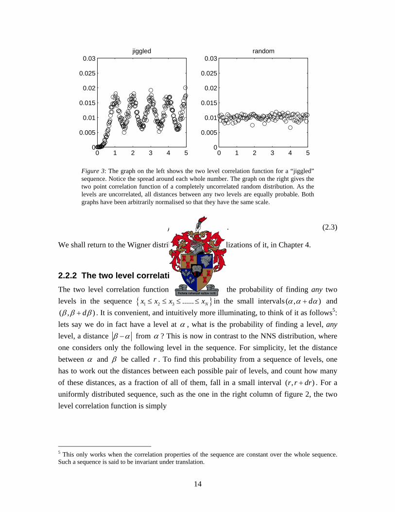
Figure 3: The graph on the left shows the two level correlation function for a “jiggled” sequence. Notice the spread around each whole number. The graph on the right gives the two point correlation function of a completely uncorrelated random distribution. As the levels are uncorrelated, all distances between any two levels are equally probable. Both graphs have been arbitrarily normalised so that they have the same scale.
0 1 2 3 4 50
0.005
0.01
0.015
0.02
0.025
0.03jiggled
0 1 2 3 4 50
0.005
0.01
0.015
0.02
0.025
0.03random
2
42( )
sss ds e ds
ππρ
−= . (2.3)
We shall return to the Wigner distribution, and generalizations of it, in Chapter 4.
2.2.2 The two level correlation function The two level correlation function, 2 ( , )X α β gives the probability of finding any two levels in the sequence { }1 2 3 ...... Nx x x x≤ ≤ ≤ ≤ in the small intervals ( , )dα α α+ and ( , )dβ β β+ . It is convenient, and intuitively more illuminating, to think of it as follows5: lets say we do in fact have a level at α , what is the probability of finding a level, any level, a distance β α− from α ? This is now in contrast to the NNS distribution, where one considers only the following level in the sequence. For simplicity, let the distance between α and β be called . To find this probability from a sequence of levels, one has to work out the distances between each possible pair of levels, and count how many of these distances, as a fraction of all of them, fall in a small interval . For a uniformly distributed sequence, such as the one in the right column of figure 2, the two level correlation function is simply
r
( , )r r dr+
5 This only works when the correlation properties of the sequence are constant over the whole sequence. Such a sequence is said to be invariant under translation.
14

20
1( ) ( )i
X rC
δ>
r i= −∑ , (2.4)
where C is some normalisation constant, which we shall not worry about at this point. Figure 3 shows the two level correlation function6, , for two other sequences. The graph on the right shows the two level correlation function of a completely uncorrelated random sequence, such as the one in the left column in figure 2. As the levels are not correlated, all inter-level distances are equally probable. Now, consider the following “jiggled”
2 ( )X r
sequence [12]: take a uniform level sequence, then “jiggle” each one of the levels by moving it up or down by a small random (Gaussian distributed, in this case) amount. The two level correlation function of such a “jiggled” sequence is shown by the graph on the left in figure 3. Notice the peaks around the integers. This is no surprise, as the “jiggled” sequence was based on a uniform level sequence with an inter-level distance of one. These peaks are an indication of correlation between levels.
2.2.3 The number variance Another way of extracting information out of a level sequence is what is called the number variance statistic. Let be the number of levels in an interval of length starting at position . The number variance is then given as follows:
( )Ln x Lx
2( ) ( ) ( )V L x LN L n x n x 2x=< > − < > , (2.5)
where denotes the average over all possible starting positions x< ⋅ > ix x= . If the level sequence has been normalised so that the average spacing between consecutive levels is one, is simply . Thus in any interval of length one expects to find ( ) xn x< > L L
( )VL N L± levels.
2.2.4 The statistic 3∆
The statistic was introduced by Dyson and Mehta in [3∆ 13], and sometimes also goes by the name of spectral rigidity. For the purpose of explanation, let us first write down the probability density of a level spectrum as a sum of Dirac delta functions:
6 Technically, the graphs depicted in figure 3 are not correlation functions, rather correlation histograms, seeing as they were constructed from a finite set of suitably generated random data.
15

Figure 4: A small part of an experimentally determined “step function” from an unfolded level sequence. The level sequence is a sequence of eigenfrequencies of a resonating quartz block. The straight line is a best fit, and one can clearly see that the levels are far from being uniformly spaced. In the part between 700 and 702 kHz, the contribution to the statistic will be smaller than the contribution due to the levels between 702 and 704 kHz.
3∆
1
1( ) ( )N
ii
x x xN
ρ δ=
= −∑ , (2.6)
where the ix ’s are the levels in the level sequence { }1 2 3 ...... Nx x x x≤ ≤ ≤ ≤ , and is the (large) number levels in the sequence. Now let us define the “step function”, more formally known as the cumulative spectral function or distribution function, of the level sequence as follows:
N
. (2.7) ( ) ( ') 'x
n x x dxρ−∞
= ∫
This function, in words, counts the number of levels smaller than . If the level sequence has been normalised that the average level spacing throughout the sequence is one, then this step function, when plotted, would look much like a straight line. The procedure of “normalising” the level sequence is called unfolding, and is not always easy to do. We shall discuss the unfolding procedure in the following section.
x
The statistic is now defined as: 3∆
23 ,
1( ) min ( ( ') ' ) 'x L
xa bL n x ax b
L+
∆ = − −∫x
dx , (2.8)
where the meaning of is the same as above. In this form the meaning of the x< ⋅ > 3∆ statistic may be a bit obscured. As mentioned earlier, for a properly unfolded spectrum, the step function will approximately be a straight line. The ( )n x 3∆ statistic measures the mean square deviation of the step function from this “best fit” straight line. For a
16

uniformly spaced level sequence, a straight line fit will be exact, and 3( )L∆ will be constant for all . For a completely random sequence, however, L 3 ( )L∆ will climb linearly with . For a sequence with level repulsion (see section 2.2.1), L 3 ( )L∆ increases as , which has been said to be the hallmark of level repulsion [6]. (log( ))O L On the practical side, there is a nice way of numerically finding the statistic for a sequence of levels [
3∆14]. Let us suppose that in the interval [ , ]x x L+ lies a sub sequence
of levels k 1 2{ , , , }kx x x… . Together with the definition 1kx x L+ = + , one can rewrite the integral in equation (2.8) in six terms that can be evaluated directly. They can be written in terms of the following:
11
( ') ' ( )kx L
jxj
1 jI n x dx j x x+
+=
= =∑∫ − , (2.9)
22
1
1' ( ') ' ( )2
kx L
jxj
21 jI x n x dx j x x
+
+=
= = ∑∫ − , (2.10)
2 23
1
1( ') ' ( )2
kx L
jxj
1 jI n x dx j x x+
+=
= = ∑∫ − , (2.11)
24
1' '2
x L
xI x dx L xL
+= = −∫ and (2.12)
(25
1( ') ' ( )3
x L
x)3 3I x dx x L x
+= = +∫ − . (2.13)
Using these equations, one can rewrite equation (2.8) for a single starting point and interval length as
xL
( )2 23 3 2 1 4 5
,
1( , ) 2 2 2mina b
L x I aI bI abI a I b LL
∆ = − − + + + . (2.14)
Lastly, the values of and for which the minimum in equation (2.14) is obtained can be calculated analytically, and are given by
a b
2 1 4 1 42
5 4
and LI I I I aIa bLI I L
− −=
−= . (2.15)
17

Finally, to find 3( )L∆ as given by equation (2.8), one has to compute 3 ( , )L x∆ for each starting point ranging over the entire spectrum, and average over them. Note however, that when choosing starting points, one should do it in such a manner that the different intervals considered do not overlap as to ensure that each contribution to the average is statistically independent.
x
2.2.5 Connection between the statistics It is interesting to note that the two level correlation function, the number variance and the statistic are all connected with one another for properly unfolded, translation invariant sequences. In contrast to the NNS distribution, the number variance and the
3∆
3∆ statistic in fact only probe two level correlations. Both of them can therefore be written in terms of the two level correlation function. The number variance in terms of the two level correlation function, as shown by Bohigas and Giannoni [11], is
. (2.16) 2( ) 2 ( )(1 ( ))L
VN L L L x X x dx= − − −∫0By algebraically finding the best fit of a straight line, 3 ( )L∆ can also be written in terms of the two level correlation function 2X as follows [9]:
3 2 23 24 0
1( ) ( ) (2 9 3 )(1 ( ))15 15
LLL L x L Lx x XL
∆ = − − − − −∫ x dx . (2.17)
Furthermore, it is shown in [15] that 3∆ statistic can in fact be written in terms of the number variance:
3 2 33 4 0
2( ) ( 2 ) ( )L
VL L L x x NL
∆ = − +∫ x dx
. (2.18)
2.3 Unfolding a sequence As discussed in section 2.1 of this chapter, Random Matrix Theory is mainly concerned not with the overall distribution of levels in a sequence, but with the fluctuations of these levels from some average level density. It therefore makes sense to eliminate the system specific7 overall level density from a sequence of levels, as has been done for the level
7 The predictions of level fluctuation properties by RMT are found in many different settings, from number theory to quantum chaos, even though each of these systems have very different overall level distributions. This universality of level fluctuations, independent of level distribution, shall be discussed in more detail later on in the thesis.
18

−2 −1 0 1 20
0.2
0.4
0.6
0.8a
E
ρ(E
)
−2 −1 0 1 20
0.2
0.4
0.6
0.8
1b
E
P(E
)
0.35 0.4 0.45 0.5 0.55
0.7
0.71
0.72
0.73
0.74
0.75
c
E
P(E
)
0 0.5 10
0.5
1
1.5d
x
ρ(x)
Figure 5: The successive steps of unfolding a sequence. Figure (a) shows the average level density of an empirical level sequence. One can clearly see that the level density varies continuously throughout the entire spectrum, the known continuous level density being shown by the solid line. Figure (b) shows the empirical cumulative density function, with the theoretically known function superimposed. Figure (c) is a close up of the indicated area in figure (b), where one can clearly see the empirical step function fluctuating around the known exact one. Finally, after the unfolding procedure has been completed, we are left with a sequence that has constant level density, as is shown in figure (d).
sequences shown in figure 2, before one starts to analyze the fluctuation properties of the sequence. In section 2.2, all the functions and statistics were defined for a level sequence that had been normalised so that the average distance between two levels was unity. Furthermore, the average distance between levels has to be constant over the whole sequence. The procedure of removing the average level density from a sequence is what is known as unfolding [6]. To illustrate the unfolding procedure, we shall work through an example. For this example, consider a level sequence 1 2 3{ }NE E E E≤ ≤ ≤ ≤… , obtained experimentally, containing a large number of levels. Let us further suppose that the exact continuous level density of this sequence is known, and is given by
19

2 2
2 2
cos( ) , ( ,( ) 2
0, ( , )
E EE
E
)π π
π π
ρ⎧ ∈ −⎪= ⎨⎪ ∉ −⎩
. (2.19)
Figure 5a shows the level density histogram of this sequence of raw data, shown by circles, and superimposed there over a solid line showing the known theoretical continuous level density. Figure 5b shows the cumulative level distribution (see (2.7)) of the level spectrum, with once again the continuous theoretical distribution superimposed. The continuous level distribution is, from (2.7) and (2.19), given by
2
2 2
( ) ( ') '
cos( ') '2
sin( ) 1, ( ,2
E
E
P E E dE
E dE
E E
π
)π π
ρ−∞
−
=
=
+= ∈
∫
∫
−
. (2.20)
Figure 5c is a close up of the small region indicated in figure 5b. One can see the variation of the step function around the theoretically known level distribution. The way one goes about to get to a constant level density is as follows: construct a new sequence, { }1 2 3 ...... Nx x x x≤ ≤ ≤ ≤ , from the original sequence by reading off the value of the continuous level distribution at each of the values 1 2 3{ }NE E E E≤ ≤ ≤ ≤… , i.e.
( ), 1, 2,3, ,i ix P E i N= = … . (2.21)
The levels in this new, unfolded level sequence all lie between 0 and 1, and the level density is now only dependent on short range fluctuations, not on the overall level distribution. This can be seen in figure 5d, where the level density histogram for the unfolded sequence is shown in the same way that the level distribution for the original data is shown in figure 5a. Notice that even though there are still fluctuations in the level density, the overall density is now constant. The step function of the new sequence now also approximates a straight line, which is needed for the application of the statistic. 3∆ In this case we knew the continuous level density, and could work from there. In practice, however, one is normally not as fortunate, and one then has to resort to obtaining an approximated continuous level density from a usually limited set of data itself. This is possible by numerical fitting and smoothing, but is unfortunately not always easy to do well.
20

3 Ensembles of random matrices
3.1 Modelling physical reality with an ensemble of matrices As discussed in the introduction, there are only relatively few simple theoretical problems that physicists can solve exactly. As the complexity of systems under investigation grow, one soon has to resort to approximation; and soon even approximation may not be able to deliver results. As a last resort, one then has to turn to a statistical approach to the problem at hand. There are in general two ways of doing this. Firstly, there is the more conventional and normally intuitively more acceptable “bottom-up” approach, whereby one constructs a statistical theory of a system taking into account all of its detailed microscopic dynamics. Then there is the other more, ad hoc “top-down” approach, where one ignores the small scale detailed dynamics, and builds the theoretical model from only a few broad physical considerations. One can then, afterward, after comparison between theoretical and experimental results, try and infer details of the unknown microscopic structure. The RMT way of doing things is, in this sense, a “top-down” approach. The RMT approach can, for most applications, be summed up as follows:
• First, define an ensemble of matrices, • secondly, try to find, analytically or numerically, some characteristics of this
theoretical ensemble, • and finally, compare the obtained characteristics of the theoretical ensemble with
experimental data. A natural question to ask is: “What are we going to learn by comparing the characteristics of some theoretical ensemble of matrices and measurements from the real world?” This is unfortunately not a simple question to answer. As we shall see in the following chapters, the success of the applicability of random matrix theory is not in question. The large and diverse spectrum of physical systems to which the level sequence predictions of random matrix theory is applicable, is remarkable. But it is this uncanny success that poses the largest, and as of yet, unsolved mystery in RMT. Why does it work? There is as of yet no system that has, to our knowledge, been approached from a fundamental first approach that has led to a “Random Matrix Theory”. The gap between the “bottom-up” approach and the “top-down” approach is still largely a mystery.
21
As we have just stated, the first step in the random matrix approach to a problem is defining an ensemble of matrices, and it is to this that we now turn. Following the idea of a “top-down” approach, one builds in the broad physical considerations of the systems that one wishes to investigate by taking them into account when constructing the ensemble of matrices. It should be constructed in such a manner that the Hamiltonian matrix of the system under consideration, and of physically similar systems, should be in a sense more probable8. Although there are many different sets of physical considerations that over the years have led to many different ensembles of random matrices, the first and probably most famous ensembles were constructed mainly by Wigner himself. These are known as the Gaussian Orthogonal, the Gaussian Unitary and the Gaussian Symplectic Ensembles. GOE, GUE and GSE for short. Wigner’s three famous ensembles were built with three distinct physical situations in mind: the GOE for systems with time reversal invariance, the GUE for systems without time reversal invariance and the GSE for systems with time reversal symmetry, but specifically where there is no rotational symmetry. In the next two sections we will introduce and discuss these three “classical” ensembles from where Random Matrix Theory for all intents and purposes got started. To get an initial feel for the basic ideas behind Random Matrix Theory, we will devote the whole of the next section to the Gaussian Orthogonal Ensemble, as it is in some respects the simplest, as well as the most physically relevant, of the three ensembles. The introduction of the GOE and the discussion of the considerations that went into its construction will also serve as an introduction to the basic ideas behind Random Matrix Theory. With the basic ideas under the belt, the Gaussian Unitary and Symplectic ensembles will then be introduced in a more compact manner in the section 3.3.
3.2 The Gaussian Orthogonal Ensemble In the literature there are many different ways that the GOE is introduced. The usual way is to write down the joint probability density function9 for the matrices in the ensemble,
8 An ensemble can be seen as a “large hat” containing a large number of items. Each of these items then has a fixed chance of being drawn from the hat associated with it. For the RMT approach, the ensemble of matrices constructed for the system at hand, should be constructed in such a way that the Hamiltonian describing it should have a relatively good chance of being “drawn from the hat”. 9 J.p.d.f. for short. The meaning of this will also become clear later in this section.
22

but we will here start by rather looking at the elements of an individual matrix from the ensemble and from there work towards the j.p.d.f. for the matrices in the ensemble. Although this approach is not as general as it should be, it is easier to understand from a practical point of view. The appropriate generalisations will be discussed in due course. Once the ensemble has been introduced, with the benefit of hindsight the considerations that originally went in to the construction of the ensemble will be discussed in some detail.
3.2.1 The elements of a matrix in the GOE Before we get to the matrices, let us first define the Gaussian distribution, as we will be needing it shortly. The probability density function of the general Gaussian distribution is given by
2 2( ) /(2
2
1( )2
xx e )µ σρπσ
− −= , (3.1)
with mean µ and variance 2σ . Now, let us construct a single matrix of the ensemble, lets say the N N× 10 matrix NA , element by element. The first requirement of the GOE is that NA be symmetric11. Due to this restriction, we will now only be free to choose ( 1) /N N 2+ of the elements, the symmetry pinning the rest of them down. For argument sake, let us suppose that we are free to choose the matrix elements of the upper triangular part of the matrix. Now, let us pick the matrix elements on the diagonal out of the Gaussian distribution with zero mean and variance 1, and the rest of the elements of the upper triangular part from the Gaussian distribution with zero mean and a variance of 1
2 . It is important to note that the probability distributions of each of the elements in the upper triangular part are independent of each other. In mathematical form we have, with denoting the matrix element in the i’
ijath row and the j’th column of the matrix NA ,
10 We will discuss the size of the matrices later on, for now it is convenient just to think of it as some fixed “not too small” large number. 11 Here symmetric means , the T denoting the transpose. This requirement of symmetry will also be discussed later on in this section.
TA A=
23

2
2
/ 21( ) , 121( ) , 1
ii
ij
aii
aij
a e i N
a e i j
ρπ
ρπ
−
−
= ≤
N
≤
= ≤ < ≤. (3.2)
3.2.2 The joint probability density function As remarked earlier in this section, an ensemble is a set of some sort of items, each having a certain probability attached to it. For the Gaussian Orthogonal Ensemble, these “items” are symmetric matrices with real valued elements, and it is to the probability attached to each of these matrices that we now turn. The probability of the individual matrix elements have already been given by equation (3.2). The question now is what the joint probability density function for a matrix in the GOE is. To be more specific, what is the probability of finding a matrix in the multi-dimensional differential volume element
iji j
dA da≤
=∏ , (3.3)
where is a vanishingly small interval containing ? Notice again that only the elements of the upper triangular part are taken into account ( i
ijda ijaj≤ ) seeing as it is only
those elements that are free to be chosen. The dimension of the volume space is thus the number of elements in the upper triangular part, ( 1) /N N 2+ for an matrix. N N× Fortunately, this not a very difficult question to answer. As the probabilities of the individual matrix elements are independent of one another, the joint probability density function is merely a product of these individual probability densities:
1 2
( ) ( ) ( )ii iji i j
A aρ ρ ρ<
⎛ ⎞⎛ ⎞= ⎜⎜ ⎟⎝ ⎠⎝ ⎠∏ ∏ a ⎟ . (3.4)
Here bracket 1 denotes the probability densities of the diagonal elements of the matrix, and bracket 2 the probability densities of the elements above the diagonal in the upper triangular part. By then substituting the probability densities of the individual matrix elements as given by equation (3.2) into equation (3.4), we obtain for an matrix: N N×
24

( )
22
22
2 2
/ 2
/ 2/ 2 ( 1) / 4
1 22/ 2 ( 1) / 4
1 1( )2
(2 )
2
ijii
ijiii ji
ii iji i j
aa
i i j
aaN N N
a aN N N
A e e
e
e
ρπ π
π π
π
<
<
−−
<
−−− − −
⎛ ⎞⎜ ⎟− +⎜ ⎟⎝ ⎠− − +
⎛ ⎞⎛ ⎞= ⎜ ⎟⎜ ⎟⎝ ⎠⎝ ⎠
∑∑ ⎛ ⎞⎛ ⎞= ⎜⎜ ⎟⎜⎝ ⎠⎝ ⎠
∑ ∑=
∏ ∏
e ⎟⎟ . (3.5)
Equation (3.5) then gives the joint probability density function for matrices in the GOE. There is however a simpler, and perhaps even more illuminating way to write it down. Taking note of the fact that the matrix A is symmetrical, consider the following:
. (3.6)
2 2 2 2 211 22 33 44
2 2 2 211 12 13 14
2 2 2 212 22 23 24
2 2 2 213 23 33 34
2 2 2 214 24 34 44
2 2
Tr( ) ( ) ( ) ( ) ( )
( )
( )
(
( )
2ii iji i j
A A A A A
a a a a
a a a a
a a a a
a a a a
a a<
= + + + +
= + + + +
+ + + + +
+ + + + +
+ + + + ++
= +∑ ∑
……………
…
)
Here denotes the trace of a matrixTr( ) 12, i.e. the sum of the diagonal elements the matrix and, for lack of better notation, 2( )ijA denotes the elements of the matrix 2A . Using (3.6) we can now rewrite equation (3.5) much more simply as follows:
21 Tr( )
1 2( )A
CA eρ−
= . (3.7)
Here all the constants in front of the exponential have been compacted into one normalization constant C , as we will not be bothered much by them. Equation (3.7) now finally shows the usual form of the j.p.d.f. given in the literature for matrices in the GOE.
3.2.3 Physical considerations built into the GOE As said before, the broad physical properties of the system to which a Random Matrix Theory approach is to be applied, is built into the ensemble of matrices. Now that we
12 The trace of a matrix is strictly speaking only defined for square matrices. We will however only encounter square matrices throughout this thesis.
25

have defined13 the GOE, it is perhaps a good time to take a look at what physical considerations went into its construction in the first place. As briefly discussed in the introduction, the physical system that Wigner was investigating when he first introduced the GOE was that of energy levels of heavy nuclei [2]. With this system in mind, let us now take a look at what went into the construction of the GOE.
3.2.3.1 Symmetry The Hamiltonian operator in the Schrödinger equation that characterizes a quantum mechanical system is required to be Hermitian. For Hamiltonians in matrix form, this implies that the Hamiltonian matrix14 of the system has to be such that H
†H H= , (3.8)
where the † operator denotes the conjugate transpose of a matrix, i.e.
† ( *)TA A= (3.9)
with the operator denoting the complex conjugate. A matrix that is its own conjugate transpose is called a Hermitian matrix.
∗
From the introduction of the GOE in section 3.2.1 it is evident that some further restriction has been made, as the matrices in the ensemble are not only Hermitian, but also symmetrical. This restriction on the possible Hamiltonians allowed in the GOE stems from a restriction on the physical systems under inspection, namely that these systems all exhibit time reversal symmetry. To get an idea of why time reversal symmetry restricts the Hamiltonian matrix of a system to being symmetrical, it may be instructive to take a brief look at the time reversal operator. When the time reversal operator acts on a system, it, by definition, reverses linear and angular momentum, but leaves position unchanged. From this it can be deduced [16] that the time reversal operator be anti-unitary. Now, an anti-unitary operator can always be
13 The GOE has been defined here more strictly than it usually is, but we will get to generalizations over and above this definition a bit later on. 14 Hamiltonians are in general matrices with complex values matrix elements. Hamiltonians with only real valued matrix elements are seen to be a special case.
26

written as the product of a unitary operator and the complex conjugation operator. In other words, for the anti-unitary time reversal operator T , we can write
0T YK= , (3.10)
with Y being a unitary operator, and denoting the complex conjugation operator. The explicit form of the time reversal operator depends on the basis that is chosen to describe the system at hand.
0K
Without going into much detail how the properties of the time reversal operator constrains the Hamiltonian of a time reversal invariant system to being symmetrical, let us consider as an example the coordinate representation specifically15. In this basis the time dependent16 Schrödinger equation can be written as follows:
2
2 ( ) ( , ) ( , )2
V x x t i x tm t
ψ ψ⎡ ⎤−
∇ + =⎢ ⎥ ∂⎣ ⎦H
∂ , (3.11)
with denoting the potential. The bracket denoted by is the Hamiltonian of the system. If one now takes the complex conjugate of both sides of equation (3.11), one obtains:
( )V x H
2
2 *( ) *( , ) *( , )2
V x x t i x tm t
ψ ψ⎡ ⎤−
∇ + = −⎢ ⎥ ∂⎣ ⎦
∂ . (3.12)
If we now replace the dummy variable with t t− , it is apparent that both ( , )x tψ and *( , )x tψ − will be solutions of the original equation (3.11) if we require that the
Hamiltonian in equation (3.12) be the same as the Hamiltonian in equation (3.11), in other words, by requiring that
( ) *( )V x V x= . (3.13)
For this to hold, it is clear that has to be real, and by implication, so too the Hamiltonian 17
( )V xH .
15 The Schrödinger equation in coordinate representation is also known as the continuous form of the Schrödinger equation. 16 As opposed to the time independent Schrödinger equation given by equation (1.1). 17 A unitary matrix that is also real, is by implication symmetrical.
27

In coordinate representation the form of the time reversal operator T , from what we have seen, is simply the complex conjugation operator:
0T K= , (3.14)
with the unitary operator Y , from equation (3.10), in this case being equal to the identity operator. In general however, Y is not equal to the identity operator, and in fact the requirement that the Hamiltonian of a system is invariant under time reversal, is given by
1THT H− = . (3.15)
For more detail in this regard, see [9] and [17]. That said, by far most quantum mechanical systems that normally occur in nature, exhibit time reversal symmetry18, making the GOE, at least from a quantum mechanical point of view, the most applicable of the three ensembles introduced by Wigner.
3.2.3.2 Invariance under basis transformation To write down the Hamiltonian of a physical system in a matrix form, it is necessary first to choose an orthonormal basis19 in which you are going to do so. There are many different ways of doing this, each leading to a seemingly different Hamiltonian matrix. In general, one can transform the Hamiltonian matrix of a system resulting from one choice of basis to a Hamiltonian for a different choice of basis by the linear transformation
H'H
1'H T HT−= , (3.16)
the only requirement on the transformation matrix T being that its inverse exists. In quantum mechanics, however, Hamiltonian matrices are always required to be Hermitian,
18 The GOE does not hold for systems exhibiting time reversal symmetry that have broken spin-reversal symmetry. An ensemble was however constructed for this special case, the GSE, which we shall briefly discuss in section 3.3.2. 19 A quantum mechanical system “lives” in a Hilbert space. When choosing a basis for this Hilbert space, it is usually done so that this basis is orthonormal, in other words the basis vectors are so chosen that they are not only orthogonal to each other, but also all have a norm of 1.
28

and will only be guarantied of being so if we further restrain the transformation matrix to being unitary. For a unitary matrix U , with the property
'H20
† † UU U U I= = , (3.17)
the transformation of basis is now
†'H U HU= . (3.18)
Taking the conjugate transpose on both sides of equation (3.18) we then have
† † †
† † †
† †
( ') ( )( ) ( ) ( )( )
'
H U HUU H UU HUH
=
=
=
†
=
, (3.19)
by using the property of conjugate transposition that for two matrices A and B
† †( ) †AB B A= , (3.20)
as well as the known fact that is Hermitian to begin with. Equation (3.19) shows that , the result of a unitary transformation of , is equal to the conjugate transpose of
itself, or is in other words, Hermitian.
H'H H
For Hamiltonian matrices describing systems with time reversal symmetry, we have to restrict the form of the transformation matrix in equation (3.16) even further. As discussed in the previous section, Hamiltonians of such systems all have the property of being symmetrical. If therefore describes a system that is invariant under time reversal, the matrix also has to be symmetrical as it too describes a system where time reversal symmetry holds. This can only be guaranteed if the transformation matrix
of equation (3.16) is even further restricted to being orthogonal. An orthogonal transformation preserves symmetry in the same way that a unitary transformation preserves Hermiticity. This can be shown in much the same as in (3.19), using the fact that for an orthogonal matrix we have
H'H
T
O
T TO O OO I= = . (3.21)
20 Here, and in the rest of the thesis, I represents the identity matrix.
29

Even though the form of a Hamiltonian matrix that describes a system is dependent on choice of basis, the actual mechanics of the physical system are not. Hamiltonian matrices that are within a unitary transformation21 of another should lead to the same, basis independent solutions of the Schrödinger equation. This brings us to an important feature of the GOE. Since matrices that are within an orthogonal transformation of one another describe the same physical system, it stands to reason that these related matrices should carry the same statistical weight in one’s ensemble. The GOE was constructed that this is indeed so. To verify this, let us take a look at the j.p.d.f. of the matrix given by equation (3.7):
'H
2
2
1 Tr( ' )1 2
1 Tr(( ) )1 2
( ')T
H
C
O HO
C
H e
e
ρ−
−
=
=
. (3.22)
Furthermore,
, (3.23)
2
2
2
2
Tr(( ) ) Tr( )Tr( )Tr( )Tr( )
T T
T
T
O HO O HOO HOO H OOO HH
=
=
=
=
T
by using equation (3.21), and the characteristic of the trace function that
Tr( ) Tr( )AB BA= (3.24)
for any two square matrices A and of equal dimension. By inserting equation (3.23) into equation (3.22), we then obtain, by comparison with equation (3.7),
B
2
2
1 Tr(( ) )1 2
1 Tr( )1 2
( ')
( )
TO HO
C
H
C
H e
eH
ρ
ρ
−
−
=
=
=
. (3.25)
Thus the j.p.d.f. for the matrix is the same as the j.p.d.f. for the matrix as we expected (hoped), as they are merely an orthogonal transformation away from another.
'H H
21 Matrices such as these are said to be unitarily equivalent.
30

3.2.3.3 Size of the matrices and Block Diagonal form The choice of basis is an important issue, as a good choice of basis may simplify the problem at hand greatly. Ideally, for example, one could choose the basis of the Hilbert space in which the system lives in such a manner that the Hamiltonian matrix of the system would simplify to a diagonal matrix, which is as simple as it gets. To do this, however, one would have to solve the Schrödinger equation, as the set of basis vectors that results in a diagonal Hamiltonian matrix, is in fact the set of allowed states of the system, i.e. the eigenstates of the Schrödinger equation in the first place. The states of the quantum mechanical system are labelled by what are called quantum numbers, each state corresponding uniquely to a unique set of quantum numbers. What these quantum numbers represent, and the way that they label the states, differs from system to system. The states of the hydrogen atom, for example, can be labelled by a set of three numbers, , representing the so called principle quantum number, representing total angular momentum, and the projection of angular momentum onto a certain fixed direction. For much more complicated systems, such as that of a heavy nucleus, labelling of individual states in such a manner is very difficult. In principle it would be possible to label all the states exactly, but that would require an exact solution of the system’s Schrödinger equation – that which we cannot do in the first place. In attempting an approximate solution, it turns out that at higher excitation levels some of the quantum numbers very quickly get washed out, as the levels get close to one another and start to mix. There are however quantum numbers that are exactly conserved throughout the spectrum – the so called good quantum numbers. For a heavy nucleus, for example, these good quantum numbers are total spin, and parity. Even though labelling individual states is not practical, it is possible to group states with the same good quantum numbers together when choosing a basis for one’s system in such a way that the Hamiltonian matrix of the system reduces to a block-diagonal form such as in figure 6. Each of these blocks can then be seen as a Hamiltonian matrix of a sub-system, and each of these smaller sub-system problems can be tackled individually. Unfortunately, these sub-problems can not be solved exactly either. It is in fact these sub-problems that Random Matrix Theory was applied to in the first place, the matrices of the GOE representing such a “sub-block” of a possible
( , , )n l m n lm
22 Hamiltonian of the entire system23.
22 Recall that, as discussed in the introduction, the Random Matrix Theory approach to a problem looks statistically at a set of different possible Hamiltonians for the system, as we cannot obtain the correct one exactly.
31

J1
J3
J2
Figure 6: A Hamiltonian matrix in block-diagonal form. In this case a basis has been chosen is such a way that each of the blocks correspond to a sub-system of states each with a fixed total angular momentum J.
In principle one would be able to define a different GOE for each integer greater than one, this whole number being the size of the matrices in the ensemble. This is not often done, as it is sufficient just to think of the GOE as a set of matrices that all have the same, large size. The reason for thinking of the size of the matrices as being large is that many of the theoretical results for the GOE, and for that matter any ensemble, can only be obtained analytically by letting the size of the matrices in the ensembles tend to infinity. It then stands to reason that the Hamiltonian matrix of the system that the GOE is intended to model, also be of large dimension24. For a heavy nucleus, as discussed above, the pure sequences that Random Matrix Theory applies to are sequences containing at least hundreds of levels, the Hamiltonian of the sub-system being of the same dimension25.
23 When comparing results from Random Matrix Theory to data from experiment, it is important that the level sequences that are considered all have the same good quantum numbers. Such a sequence is called a pure sequence. 24 The meaning of this will become clearer in the next chapter, as we will be discussing theoretical results of the GOE, and other ensembles, in more detail. Examples will be given of the dependence of these results on the size of the matrices in the ensembles. 25 Here it is meant in the sense that, if there were N levels in the sequence, the corresponding Hamiltonian of the sub-system would be an NxN matrix.
32
3.2.4 A not so physical consideration and how it was fixed By implication, when one is attempting an approximate solution to a given physical problem, some physically relevant information has to be left out. The trick of a good approximation is leaving out the least relevant information that will un-complicate the problem most. Sometimes, however, assumptions are made to simplify a problem that have no physical basis at all, and even be counter to physical assumption in some way. One such feature has been built into the GOE, purely as an assumption to make the ensemble analytically more tractable, and it is this feature that we will now briefly take a look at.
3.2.4.1 Independence of matrix elements The j.p.d.f. of the matrices in the GOE given by equation (3.7) is in fact a special case of the following more general form:
2( Tr( ) Tr( ) )1( ) a H b H c
CH eρ − + += , (3.26)
with , and real numbers, with a required to be positivea b c 26. The constant is once again a normalization constant that will not bother us much. In 1960 Porter and Rosenzweig [
C
18] proved that if one is to require that the matrix elements of the matrices in an ensemble be independently distributed, and also require that the resulting j.p.d.f. be invariant under orthogonal transformation, the j.p.d.f. is automatically restricted to what is given by equation (3.26). As discussed in section 3.2.3.2, the requirement of the j.p.d.f. being invariant under transformation of basis is certainly justifiable from a physical point of view, but the requirement of the matrix elements being independently distributed is not. It was merely for the purpose of making the GOE amendable to an analytical treatment.
3.2.4.2 The Circular Ensembles It is not only the lack of physical motivation for the independence of matrix elements that posed a problem, but in fact that it was against the premise of Random Matrix Theory. Dyson argued [4] that an ensemble of matrices should be constructed in such a way that
26 In principle there is thus a distinct GOE for every conceivable choice of a, b and c. One is free to make this choice as one likes, however, as one can switch between these “different” ensembles simply by a change of variables, all leading to the same results discussed in chapter 4.
33
“all interactions are equally probable”, and that it was impossible to do if the matrix elements were required to be independent of one another. This then led him to construct his famous “circular ensembles”, intended to model systems with the same physical considerations as Wigner’s ensembles, but without the added requirement of independent matrix elements. He also did it in such a way that the ensemble remained analytically tractable. One might now ask the question why we still bother with Wigner’s ensembles if those of Dyson are physically more justifiable. The remarkable fact is that the analytic results obtained form Wigner’s Gaussian ensembles and those from Dyson’s Circular ensembles are the same [4]. This was the first indication of an important concept in Random Matrix Theory called “universality” that is still today not fully understood. To get an intuitive understanding of this universality, we will first need to take a look at these so called analytical results. We will be doing so in the next chapter, where the idea of universality will arise in more detail.
3.3 The Gaussian Unitary and Symplectic ensembles As most of the basic concepts have been covered in the introduction of the GOE, the introduction of the other two ensembles that Wigner constructed will be much more brief. These other two ensembles, constructed by Wigner with two distinct physical systems in mind, are known as the Gaussian Unitary and the Gaussian Symplectic ensembles. It is to these ensembles that we now turn.
3.3.1 The Gaussian Unitary Ensemble Where the GOE was constructed for systems with time reversal invariance, the GUE was constructed for systems that do not have this property. It is in principle “easy” to create a quantum mechanical system without time reversal symmetry – one just has to place a system that has time reversal symmetry in a strong external magnetic field. In practice, this was not at all easy at the time that the ensembles were first constructed, as the magnetic fields required to sufficiently “break” time reversal symmetry of atomic nuclei systems were not experimentally possible. Dyson did however mention [4] the possibility of future application to atomic and molecular systems. The GUE has indeed proven to be a very useful ensemble, finding applications far away from the nuclear systems it was
34

originally intended for. Furthermore, the GUE also turned out to be the easiest of Wigner’s to handle analytically, as we shall see in the next chapter. As just stated, the difference between the GOE and GUE lies in the requirement of time reversal symmetry. As we have discussed in section 3.2.3.1, systems with time reversal symmetry have symmetric Hamiltonian matrices describing them, and it is therefore symmetric matrices that the GOE is built up of. Without the requirement of time reversal symmetry, all one can say about Hamiltonian matrices of such systems is that they are Hermitian, and the GUE is therefore simply built out of Hermitian matrices. Other than that, the further requirements on matrices in the GUE are the same as those on matrices in the GOE. Just as the GOE, the matrices in the GUE are such that their individual matrix elements are independently distributed. As the matrices in the GOE were required to be symmetric, the individual matrix elements were restricted to being real. With the requirement on matrices in the GUE being weakened to Hermiticity, the individual matrix elements, except for those on the diagonal, can now in general have complex values. Let us suppose that the matrix elements of a Hermitian matrix A , once again of size , is given by N N×
ij ij ija x iy= + . (3.27)
The requirement of Hermiticity does restrict the possible values of the matrix elements. As just mentioned, the elements on the diagonal of a Hermitian matrix cannot have a complex value. From the definition of Hermiticity by equations (3.8) and (3.9) one can first of all deduce that the matrix elements on the diagonal of a Hermitian matrix are restricted to having real values, or in other words
0, 1..iiy i N= = . (3.28)
Secondly the matrix elements opposite of the diagonal from each other are related by
. (3.29) *ij jia a=
Restrictions (3.28) and (3.29) imply that, just as with the symmetric matrices in the GOE, not all the matrix elements are free to be chosen. Let us, once again for argument sake, suppose that the matrix elements that we are free to choose are those lying in the upper triangular part of the matrix, restrictions (3.28) and (3.29) pinning the rest of them down so to speak. As with the GOE, the “free” elements are required to be independently
35

distributed, but in this case with the added meaning that the real and imaginary parts of the matrix elements also be independent of each other. All this considered, an N N× matrix thus has elements that are free to be chosen, of them lying on the diagonal, and
2N N( )2 ( 1) / 2 (N N N N× − = −1) lying above the diagonal. The j.p.d.f. thus gives the
probability of finding matrix A of the GUE in the differential volume element
1
ii ij iji i j i j
dA dx dx dy< <
⎛ ⎞⎛⎛ ⎞= ⎜ ⎟⎜⎜ ⎟⎝ ⎠⎝ ⎠⎝∏ ∏ ∏
2
⎞⎟⎠
, (3.30)
with and denoting vanishingly small intervals in the regions of ijdx ijdy ijx and respectively. Bracket one represents the elements on the diagonal, and bracket two the elements above the diagonal in the upper triangular part. Note that this volume element has a dimension of .
ijy
2N The general form of the j.p.d.f. of matrices in the GUE is identical to that of the GOE, as given by equation (3.26), the only difference being that it now refers to Hermitian matrices instead of symmetric ones. Just as was the case for the GOE, one is free to “choose” the constants in equation (3.26) as one likes, as the properties that are of interest27 are independent of this choice. It is thus convenient, for practical purposes, to once again take the diagonal elements of the matrices in the GUE from a Gaussian distribution with mean 0 and variance 1, and the elements above the diagonal in the upper triangular part from a Gaussian distribution with mean 0 and variance ½. This choice of matrix elements then leads to, in analogy with that of the GOE, the following normalized j.p.d.f. for matrices of size : N N×
( )222 2
1 Tr2( ) 2
N N AA eρ π
−− −= . (3.31)
3.3.2 The Gaussian Symplectic Ensemble As mentioned in section 3.2.3.1, there is a special class of quantum mechanical systems that exhibit time reversal symmetry that the GOE does not apply to. These are systems with half-integer total angular momentum that are not symmetrical under rotation28. For such systems such a specific ensemble was created, known as the Gaussian Symplectic
27 Some of these properties will be discussed in chapter 4. 28 As an example, systems with strong spin-orbit coupling adhere to GSE statistics.
36

Ensemble. In quantum mechanics all Hamiltonian matrices are required to be Hermitian. Where the matrices of the GOE have been further constrained to being symmetrical, the constituents of the GSE are constrained to being real quaternion matrices. Any matrix with complex valued entries can be expressed as a linear combination of the following four matrices:
2 2×
(3.32) 0 1 2 3
1 0 0 0 1 0, , ,
0 1 0 1 0 0i i
E E E Ei i
−⎡ ⎤ ⎡ ⎤ ⎡ ⎤ ⎡= = = =⎢ ⎥ ⎢ ⎥ ⎢ ⎥ ⎢ −⎣ ⎦ ⎣ ⎦ ⎣ ⎦ ⎣
,⎤⎥⎦
In other words, one can write any complex valued 2 2× matrix Q as
, (3.33) 3
n nQ c E=
= ∑0n
the coefficients in general being complex numbers. If however they are real, the matrix is said to be a real quaternion. It is important to note that, even though called real quaternion, such a matrix does not in general have only real valued entries.
ncQ
A real quaternion matrix is constructed out of N N× H N N× real quaternion 2 2× matrices such as depicted in equation (3.33). Counting the individual matrix elements, it is evident that the dimension of is in fact H 2 2N N× . For the matrix to also be Hermitian, one has to be able to write it as follows:
H
, (3.34) 0 0 1 1 2 2 3H H E H E H E H E= ⊗ + ⊗ + ⊗ + ⊗ 3
with a real symmetric matrix, and , and real anti-symmetric matrices. Here the
0H N N× 1H 2H 3H⊗ operator denotes the direct product. To get a feel for all of this, let
us as an example construct a 2 Hermitian real quaternion matrix. For the matrices 2×
(3.35) 0 1 2 3
0 0 0, , ,
0 0a c d f g
H H H Hc b d f g⎡ ⎤ ⎡ ⎤ ⎡ ⎤ ⎡
= = = =⎢ ⎥ ⎢ ⎥ ⎢ ⎥ ⎢− − −⎣ ⎦ ⎣ ⎦ ⎣ ⎦ ⎣,
0⎤⎥⎦
id
⎥⎥
we have
, (3.36)
00
00
a b ig fa f id b ig
Hb ig f id bf id b ig b
+ − +⎡ ⎤⎢ ⎥+ −⎢=⎢ − −⎢ ⎥− − +⎣ ⎦
37

with , b , c , , a d f and all real numbers. g As is a real symmetric matrix, it has 0H ( 1) /N N 2+ free parameters, and as , and
are real anti-symmetric matrices, they each have 1H 2H
3H ( 1) /N N 2− free parameters. Adding this all up, a real quaternion matrix therefore has free parameters, and for matrices in the GSE, these are once again required to be independently distributed. If the distribution of the matrix elements are Gaussian, the resultant j.p.d.f. for matrices in the GSE, just as for the GOE and GUE, has the general form given by equation (3.26).
N N× 22N N−
Where the j.p.d.f. of the GOE is invariant under orthogonal transformations, the j.p.d.f. of the GSE is invariant under symplectic unitary transformations, brought about by transformation matrices from the symplectic unitary group. A matrix is a member of this group if it satisfies the identity
B
TZ BZB= , (3.37)
the matrix Z defined by
2Z I E= ⊗ (3.38)
with I the identity matrix. For more detail in this regard, see section 2.4 in [9]. N N×
3.4 More ensembles Since Wigner’s introduction of the GOE, the GUE and GSE, a very large variety of ensembles have been constructed. Some of these ensembles were put together with specific systems in mind, and some were considered merely on a theoretical basis as Random Matrix Theory developed into a field of research in its own right. With this in mind we will now briefly introduce two more ensembles, or rather concepts, that we will encounter later on in this thesis.
3.4.1 The Crossover between GOE and GUE In general, an ensemble of random matrices is constructed for systems having specific physical attributes. If one were to then investigate a system, and find that its experimental properties match that of some ensemble, it stands to reason that one would be able to assume that the original physical considerations built into the matching ensemble also
38

apply to the physical system under consideration. To illustrate this idea, we will here briefly discuss an example. As mentioned earlier on, one can create a system with broken time reversal symmetry by placing a system with time reversal symmetry in a strong external magnetic field. This magnetic field then effectively breaks the time reversal symmetry of the system, the level statistics no longer adhering to that of the GOE, but of the GUE. If one were however to slowly turn on the external magnetic field, the transition from GOE to GUE statistics would not be instantaneous, rather gradual with the increasing magnetic field. To study this transition, Pandey and Mehta [19] introduced an ensemble of matrices, discussed in Mehta’s book [9], with Gaussian element densities to interpolate between the GOE and the GUE, the ensembles constructed in the first place to model systems with and without time reversal symmetry respectively. In general it possible to break up any Hermitian matrix A into two real valued matrices – one being symmetric and the other anti-symmetric. In other words, one can write for A
0 1A A iA= + , (3.39)
with 0A a symmetric matrix and 1A an anti-symmetric one. Now in order to model the Hamiltonian of a system where the time reversal symmetry is “almost conserved”, it stands to reason that it would have a Hamiltonian matrix that is almost symmetrical, in the sense that its anti-symmetric part will be close to zero relative to the symmetric part. By strengthening the magnetic field, time reversal symmetry will be broken even more, resulting in the anti-symmetric part of the Hamiltonian matrix becoming more predominant. The question now is how predominant the anti-symmetric part of a system’s Hamiltonian matrix has to become for time reversal symmetry to be completely broken. To get the idea of how this can be done, consider the following matrix
0H H iH1α= + , (3.40)
with the matrix a symmetric matrix and an anti-symmetric one, both of them with matrix elements that are identically distributed, all with the same Gaussian distributions. The parameter
0H 1H
α can now be adjusted so that varies from perfectly symmetric, with H0α = , to a matrix that is “completely Hermitian”, with 1α = . With matrices such as
39

these it is then possible to construct an ensemble that interpolates between the GOE and GUE, with the j.p.d.f. given by
( 20 1Tr ( )1
( )( ) a H iHCH e α α
αρ − += ) , (3.41)
with the constants and both dependent on a C α 29. By now adjusting the parameterα , it is possible to interpolate between the GOE and GUE, 0α = resulting in the GOE and
1α = resulting in the GUE. Irrespective of the choice of α , the resulting ensemble adheres to all the requirements imposed on the GOE, even being invariant under orthogonal transformation.
3.4.2 More general ensembles As we have seen earlier on in this chapter, by requiring an ensemble to have matrices with matrix elements that are independently distributed and also to have a j.p.d.f. that is invariant under a transformation of basis, the j.p.d.f. of the ensemble is restricted to the form given by equation (3.26) as
2( Tr( ) Tr( ) )1( ) a H b H c
CH eρ − + += ,
for a matrix in the ensemble. The requirement on the j.p.d.f. to be independent from basis transformations has a clear physical motivation, but the requirement of independently distributed matrix elements does not. As there was originally no reason to make this requirement other than to make the resulting ensembles easier to handle analytically, one could ask what ensembles would result if this restriction had not been made in the first place. By dropping the requirement of independently distributed matrix elements when constructing an ensemble, the form of the j.p.d.f. is now no longer required to be given by equation (3.26). One possible way to generalize the form that the j.p.d.f. of an ensemble may take
H
30 that will be important later on, is
Tr( ( ))1( ) V HH eρ −= C
, (3.42)
29 This is done in such a way that the j.p.d.f. stays normalized, and that the variance of the eigenvalues of the matrices in the ensemble remain the same. 30 There are many other ways of constructing ensembles that are not bound by the requirement of independently distributed matrix elements. Dyson’s circular ensembles, for example, also do not have this requirement.
40
with being some function of . The form of is normally restricted to being a polynomial function where the highest power is even, and its coefficient positive.
( )V H H ( )V H
It is important to note that a j.p.d.f. with the general form of equation (3.42) is still independent of a transformation of basis. The reason for this being that the trace of any power of a matrix is independent of a transformation of basis, which can be proven by an inductive extension of the proof for the special case of the square of a matrix, given by equation (3.23). By applying this fact to each power of the polynomial function , it is then easy to see that the general j.p.d.f. given equation (3.42) is invariant under transformation of basis.
( )V H
An interesting note is that it has been proven [20] that all invariants under a transformation of basis of an matrix can be expressed in terms of traces of the first
powers of the matrix. N N×
N
3.5 Summary In this chapter we have covered many basic aspects of ensembles of random matrices, and in doing so also some aspects of Random Matrix Theory as a whole. As the discussion has in general been broad, we here review the most important points discussed to help put them in perspective.
3.5.1 Why ensembles of random matrices? The basic idea of Random Matrix Theory is to presume that the unobtainable Hamiltonian matrix of a system under inspection is one of some ensemble of possible Hamiltonian matrices. Now, instead of trying to find the specific Hamiltonian in question, one studies the properties of this ensemble of matrices, hoping that these properties will be the same as, or at least close to, the properties of the specific but unknown Hamiltonian matrix of the system in question. It is clear that the success of the Random Matrix Theory approach lies in the right choice of ensemble of matrices, right meaning that the ensemble be chosen in such a way that the Hamiltonian matrix of the system in question, and those of similar systems, be in a sense the most probable ones in the ensemble. The first to approach a problem in this way was Wigner, and it is his Gaussian ensembles that form the entry point to Random Matrix Theory.
41

3.5.2 Considerations built into the Gaussian ensembles The three classical ensembles constructed by Wigner are the GOE, the GUE and the GSE. All three ensembles were built on the following considerations:
1. Independently distributed matrix elements The matrices in the ensemble are made up of matrix elements that are independently distributed of one another. This requirement was imposed solely for the purpose of making the ensembles easier to handle analytically.
2. Invariance under transformation of basis In an ensemble, each element in it has associated with it a probability. For ensembles of matrices, this is called the joint probability density function, or j.p.d.f. for short. It is required that the j.p.d.f. for matrices in the ensemble that are within a basis transformation of each other be the same, in other words invariant under transformation of basis. This requirement was made due to the physical consideration that the dynamics of a system are not dependent on the choice of basis used to describe it.
3. Symmetry It is here that the difference between the ensembles lies. They were constructed with three distinct groups of systems in mind, the systems being grouped by the same broad physical symmetries. The three groups, and the ensembles that were built for them, are
• The GOE – Systems with time reversal invariance as well as integer spin, with or without rotational symmetry, or half integer spin with rotational symmetry.
• The GSE – Systems with time reversal invariance as well as half integer spin with broken rotational symmetry.
• The GUE – Systems with broken time reversal invariance. It is important to first of all distinguish between systems with time reversal symmetry, and systems without it. For systems without it, the GUE is the applicable ensemble. Systems with time reversal symmetry are, however, split into two subgroups, corresponding to the GOE and the GSE. The GOE covers virtually all systems with time reversal invariance, the exception being systems
42
that also have half integer spin and broken rotational symmetry. This subgroup of systems is then covered by the GSE.
3.5.3 How the considerations were built into the Gaussian ensembles Each of the three considerations mentioned above manifest themselves in different aspects of the ensembles. Briefly summarized, it is as follows:
1. Invariance under transformation of basis The j.p.d.f. of the matrices in the ensembles is required to be invariant under transformation of basis. A general form that adheres to this requirement is (equation (3.42))
Tr( ( ))1( ) V HH eρ −= C .
This is thanks to the taking of the trace of the function of in the exponent of the j.p.d.f.. It is important to note that the function V is normally required to be a finite even polynomial, with the coefficient of the leading power restricted to be a positive number. This is to ensure that the j.p.d.f. has a finite norm.
H
2. Independently distributed matrix elements
This feature manifests itself simply as stated. Together with the requirement of independence under basis transformation, it does however restrict the possible j.p.d.f. for an ensemble to a very specific form, i.e. (equation (3.26))
2( Tr( ) Tr( ) )1( ) a H b H cH eρ C
− + += .
As the coefficient of the leading power, is restricted to be a positive number. With the j.p.d.f. restricted to the form of a Gaussian distribution, Wigner’s ensembles were called the Gaussian ensembles.
a
3. Symmetry
The three different symmetry requirements manifest themselves in different symmetry requirements on the constituent matrices of each of the three ensembles.
• The GUE is built out of matrices that are plainly Hermitian. • The GOE is built out of matrices that are symmetrical.
43

• The GSE is built out of matrices that are real quaternion. It is important to note that in general the Hamiltonian matrices of quantum mechanical systems are restricted to be Hermitian, therefore the matrices in the GOE and GSE are first of all also Hermitian. The symmetries of the systems under consideration however further restrict the possible form of their Hamiltonian matrices, leading to the stricter conditions of the matrices in the ensembles being required to be symmetrical and real quaternion respectively.
Another important note is that the requirement of independence under transformation of basis is related to the symmetry requirements, in the sense that the possible transformation matrices, which bring about basis transformations, are also restricted. For the GOE, this means that the transformation matrices have to be orthogonal, and for the GSE the transformation matrices have to be from the symplectic unitary group. As for the GUE, the transformation only has to be unitary. It is clear that the ensembles were also named with this in mind.
Finally, note that even though the constituent matrices obey different symmetries, the j.p.d.f. of the three ensembles still all have the general form given by equation (3.26).
3.5.4 A few practical notes In practice one may want to construct individual matrices of an ensemble for, say, numerical experiments31. This may be hard to do directly from the j.p.d.f. of the ensemble. It would be much easier to construct a matrix of an ensemble element by element, and fortunately, at least for the Gaussian ensembles, this is possible to do. We will here summarize how to do this for the GOE and the GUE. It is also possible to do for the GSE, but due to the unusual symmetry requirement of its constituent matrices, is a little more complicated.
The GOE Due to the requirement on the matrices to be symmetrical, the matrix elements are restricted to be real. Construct the matrix by taking diagonal elements from a
31 If one would want to estimate some ensemble average numerically, it is much easier to directly average over matrices taken directly from the ensemble, than by first having to work out the probability of finding each of a set of “test” matrices in the ensemble in the first place.
44

Gaussian distribution with mean 0 and variance 1, and the rest of the elements of the upper triangular part from a Gaussian distribution with mean 0 and variance ½. The rest of the matrix elements are fixed by the symmetry of the matrix. This then leads to the following normalized j.p.d.f. for an N N× matrix (equation (3.5)):
H
( ) ( )21 Tr/ 2 ( 1) / 4 2( ) 2
HN N NH eρ π
−− − += .
The GUE Without the matrices being required to be symmetric, the matrix elements can now, in general, be complex. The matrices are however required to be Hermitian, restricting the diagonal elements of the matrices to be real. Once again construct the matrix by taking diagonal elements from a Gaussian distribution with mean 0 and variance 1, and the rest of the elements of the upper triangular half from a Gaussian distribution with mean 0 and variance ½. The rest of the matrix elements are now pinned down by the requirement that the matrix be Hermitian. Note that by taking a complex number from a distribution we mean that the real and imaginary parts of the complex number are taken independently from the same distribution. This then leads to the following normalized j.p.d.f. for an
matrix (equation (3.31)): N N× H
( ) ( )22
1 Tr/ 2 / 2 2( ) 2HN NH eρ π
−− −= .
The j.p.d.f.’s given here for the GOE and the GUE, and for that matter also of the GSE, all adhere to the general form given by equation (3.26). Just as it is by a transformation of variables possible to transform a general Gaussian distribution with arbitrary mean and variance to the “standard” Gaussian distribution with mean 0 and variance 1, one can transform the general form of the j.p.d.f. given by equation (3.26) to a form that more resembles the ones that are given here. The theoretical results obtained for all possible choices of j.p.d.f. adhering to equation (3.26) are the same, and it is therefore sufficient to study the simpler forms given here. When constructing these matrices for the purpose of numerical experiment, one has to at some stage decide on a size for them. The dependence of ensemble averages on the size
45

of the matrices in the ensembles will be discussed in some detail in the following chapter. In principle one can choose any size one likes, just as long as it is the same for all the matrices in the ensemble. It is however normally the case that the system one is intending to model with an ensemble of matrices lives in a very large dimensional space, and consequently has a Hamiltonian matrix of large dimension. Furthermore, most theoretical results obtained from the ensembles are done so by letting the size of the matrices tend to infinity. All this considered, it therefore stands to reason that the matrices in one’s ensemble should then also be of large dimension.
46

4 Level statistics of random matrix ensembles
4.1 Comparing theory and experiment In the previous chapter we defined and discussed different ensembles of random matrices. Unfortunately this discussion had to be kept rather theoretical in nature, only here and there alluding to a comparison between properties of an ensemble and experimental results. Now that we have the basic ideas of ensembles of random matrices behind us, we can finally get to discussing their properties; and in so doing make the connection to the physical world. It goes without saying that there are many different aspects of random matrix ensembles, some of them being more relevant to physical systems than others. It is the purpose of this chapter to investigate some of the more relevant properties that have been discussed in the literature, and by doing so also giving a brief tour of some of the applications of Random Matrix Theory. As before, we will along the way come across some broad principles that are important to Random Matrix Theory, and will discuss them in due course. As mentioned earlier, the predictions of Random Matrix Theory are classically concerned with level sequences, or to be more specific, correlations between levels in a sequence of levels. In chapter 2 we reviewed a few properties of level sequences in general, and these are the same level sequence properties that we will be discussing in this chapter. This time however we will be averaging them over entire ensembles of level sequences. Recall that these properties, or rather statistics, of level sequences were designed for studying the local correlations between levels, rather than the global distribution of levels. For this reason we also in chapter 2 discussed the procedure for unfolding a sequence of levels, leaving it with a constant level density throughout the spectrum. The average level density is said to be a global property of a sequence of levels, whereas the statistics discussed in chapter 2, such as the NNS distribution of a sequence, is said to probe local properties of a sequence. The local properties of a level sequence are sometimes referred to in the literature as the fluctuation properties of a spectrum, and it is specifically these properties that concern Random Matrix Theory. To get a taste of what lies ahead, let us briefly take a look at an example. It was in the field of nuclear physics that experimental data first became good enough to make statistically significant comparisons to predictions made by Random Matrix Theory.
47

Figure 7: This figure shows a histogram of nearest neighbour spacings for energy levels taken from the Nuclear Data Ensemble, containing data of the energy level sequences of many different heavy nuclei. Superimposed on this histogram is the NNS distribution as predicted from the GOE, and also the Poisson distribution for reference. The fit of the GOE NNS to the experimental data is remarkable. The figure is taken from [21].
Figure 7 shows a histogram of nearest neighbour spacings for energy levels of heavy nuclei, taken from the Nuclear Data Ensemble, or NDE for short32. Superimposed over this is the nearest neighbour spacing distribution as predicted from the GOE. As one can see, the similarity is remarkable, especially when taking into account how little physical information went into the construction of the GOE in the first place. It is even more astonishing considering that built into the GOE is an assumption that is not even in line with physical reality in the first place. As we shall see throughout this chapter, it is not only in the field of nuclear physics where predictions of Random Matrix Theory have done so remarkably well. Once again the focus will be, for the most part, on the Gaussian ensembles as their properties are probably most well known, and the study of them forms the basis of classical Random Matrix Theory.
4.2 The eigenvalue joint probability density function As we have just mentioned, Random Matrix theory is mainly concerned with properties of sequences of levels. Since the 1950’s these sequences have come to represent many
32 The NDE is a famous ensemble of nuclear energy level spectra, obtained experimentally from many different heavy nuclei. Of course, for the histogram in figure six, these spectra were all unfolded and normalized to have the same average inter level distance.
48

different things in many different fields of study, but it is a good idea to, for now, still think of them as representing energy levels of a quantum mechanical system just as Wigner did originally. In this light remember that each matrix in an ensemble represents a possible Hamiltonian matrix of a system. Now, each of these matrices has it own set of eigenvalues, and just as the matrices represent possible Hamiltonians of a system, the sets of eigenvalues represent possible energy spectra of the system – giving rise to the idea of an ensemble of level sequences. Obviously only the set of eigenvalues corresponding to the correct Hamiltonian matrix33 will give the energy levels of the system exactly, but in the spirit of Random Matrix Theory it is hoped that all the sequences of eigenvalues in the relevant ensemble will share the same general properties. In other words, we hope that the specific properties of most eigenvalue sequences in an ensemble will be more or less the same as these properties averaged over the entire ensemble. The main purpose of this chapter is the introduction of some of these ensemble averaged properties of the Gaussian ensembles. Before we get to them, however, we will first need to write down a j.p.d.f. for finding a specific sequence of eigenvalues in an ensemble. Before we get started, let us first clarify what is meant by a j.p.d.f. for sequences of eigenvalues. The j.p.d.f. we are looking for gives the probability that the eigenvalue sequence of a matrix taken from some ensemble will lie in the multidimensional differential volume element
idX dx=i∏ , (4.1)
in other words, be such that each eigenvalue lies in its own differential interval centred around
idx
ix .
4.2.1 A change of variables The first step in finding the eigenvalue j.p.d.f. for one of the Gaussian ensembles, is to rewrite the familiar matrix element j.p.d.f. for matrices in an ensemble in terms of a new set of variables. Obviously the success of this depends on choosing the right set of new variables, and it is to this choice that we will now turn.
33 Stated more carefully, matrices that are within a transformation of basis of each other share the same set of eigenvalues.
49

Probably the most important property of Hermitian matrices34 is that any Hermitian matrix can be diagonalized uniquely by a unitary transformation. To be more specific, for any Hermitian matrix there exists a unitary matrix U and a diagonal matrix
such that N N× H
X
†H U XU= , (4.2)
and there is only one way in which this can be done. It turns out that the non-zero elements of the diagonal matrix are real values given by the eigenvalues of , and the transformation matrix by its eigenvectors, each column of U being a normalized eigenvector of . Seeing as each Hermitian matrix can be written uniquely in the form of equation (4.2), it is possible to, instead of specifying individual matrix elements, specify the matrices and U to determine it completely. being a diagonal matrix, it can be fully determined by real parameters, these then being the eigenvalues of the matrix. For the transformation matrix U this is a bit more complicated as, due to the constraint of unitarity, its matrix elements are dependent on each other. We can, however, easily enough count how many real parameters will be required to specify it, by simply counting variables. As an example, consider matrices of the GOE. As they are symmetric, each of them are specified by
H
H H
X XN
( 1) / 2N N + real parameters. For the new set of parameters, N of them are used up in determining the diagonal matrix, leaving only for specifying the transformation matrix. Note that in this case the transformation matrix would not only be unitary, but orthogonal. We will not go into detail as to how to specify the unitary transformation matrices in equation (4.2), we just note that it can be done. To summarize, instead of specifying a Hermitian matrix by its matrix elements , one can do it with a set of parameters specifying the transformation matrix that diagonalizes , together with its set of eigenvalues
( 1) /N N − 2
H { }ijh
1 2 3{ , , , }u u u …H 1 2{ , , }Nx x x… .
The importance of this new set of parameters lies in the fact that once the transformation of the j.p.d.f. to them has been made, its dependence upon the eigenvalues of the matrix will become apparent, hopefully leading to the eigenvalue j.p.d.f. that we are after. As it turns out, it does.
34 The fact that one can always diagonalize a Hermitian matrix and that this diagonalization always leads to real eigenvalues, are the main reasons that in quantum mechanics Hamiltonian matrices are required to be Hermitian.
50

4.2.2 The eigenvalue j.p.d.f Throughout chapter 3 we encountered various forms of the matrix element j.p.d.f. for matrices of the Gaussian ensembles; the most general form given by equation (3.26). As stated before, any choice of j.p.d.f. adhering to this general form has the same general properties, as one can jump between them merely by a change of variables. Later on in this chapter we will consider even more general forms of j.p.d.f. than that given by equation (3.26), but for now, let us just consider a j.p.d.f. of with the form
2Tr( )1( ) a HH eρ −= C . (4.3)
Applying the transformation given by equation (4.2) to this gives
( )
( )
( )
2
2
Tr ( )1
Tr ( )1
Tr1
( )T
T T
a U XUC
a U XUU XUC
a XC
H e
e
e
ρ −
−
−
=
=
=
. (4.4)
This is no surprise, as diagonalizing a matrix is merely a special form of unitary transformation, and as we know this leaves the j.p.d.f. of the matrix untouched. being a diagonal matrix, however does simplify things, as
X
2Tr( ) ii
2X x=∑ , (4.5)
the ix ’s being the eigenvalues of the matrix . It would seem that we are done, the j.p.d.f. now in terms of the eigenvalues of the matrix, and as we would have expected, independent of the parameters needed to specify the transformation matrix U .
H
Unfortunately things are not quite as simple as that. Remember that ( )Hρ in equation (4.4) is merely a probability density function. To get a probability distribution, it needs to be integrated over. The ( )Hρ given by equation (4.4), although in terms of the eigenvalues of , still gives the probability of finding the matrix in a differential volume element specified by the matrix elements
H H35. To rewrite a probability density
function in terms of new variables, one has therefore also take into account the transformation to a new differential volume element. This type of transformation is well known however, and is done as follows:
35 The differential volume elements corresponding to the GOE and GUE j.p.d.f.’s are given by equations (3.3) and (3.30) respectively.
51

. (4.6) ({ },{ }) ( )( )ij i i i ii j i i
dh J x u dx du≤
=∏ ∏ ∏
Here J represents what is called the Jacobian of the transformation, and is in the case of the GOE given by
11 12
1 1
11 12
2 2
11 12
( 1) / 2 ( 1) / 2 ( 1) / 2
11 12
1 1
11 12
2 2
11 12
NN
NN
NN
N N N N N N
NN
NN
NN
N N
hh hu u u
hh hu u u
hh hu u u
hh hx x x
hh hx x x
hh hx x x
− −
∂∂ ∂∂ ∂ ∂
∂∂ ∂∂ ∂ ∂
∂∂ ∂∂ ∂ ∂
∂∂ ∂∂ ∂ ∂
∂∂ ∂∂ ∂ ∂
∂∂ ∂∂ ∂ ∂
1
2
1
2
N
−
, (4.7)
which, as one can see, is the determinant of a ( ) ( )( 1) / 2 ( 1) / 2N N N N+ × + dimensional matrix. The important thing to note, however, is that the Jacobian is here explicitly in terms of the parameters { }ix and { . As it turns out, it can be simplified quite nicely. How this is done is a rather hairy business, the details of which can be found, for instance, in Mehta’s book [9]. For the GOE, the Jacobian in its simplified form is given by
}iu
({ },{ }) ({ })i i i ji j
iJ x u f u x x<
= −∏ . (4.8)
The main thing to notice is that Jacobian factorizes into two parts – one that depends on the parameters { , and the other on the eigenvalues {}iu }ix . We now finally have all the tools needed to make the transformation of variables
52

. (4.9) { } { },{ }ij i ih x→ u
In terms of the old variables, we have for the probability distribution ({ })ijP h
. (4.10) ({ }) ( ) ( )ij iji j
P h dh Hρ≤
= ⌠⎮⌡ ∏
Using equations (4.5) and (4.4) to rewrite ( )Hρ in terms of the eigenvalues { }ix , and transforming to the new differential volume element with equations (4.8) and (4.6), we can finally rewrite equation (4.10) in terms of the new variables:
2
({ },{ }) ( ) ({ },{ })
1 ( ) ({ })i
i
i i i i i ii i
a x
i i i j ii i i j
P x u dx du J x u
dx du f u x x eC
ρ
−
<
=
∑⎛= −⎜ ⎟
⎝ ⎠
⌠⌡
⌠⎮⌡
∏ ∏
∏ ∏ ∏⎞ . (4.11)
As the Jacobian’s dependence on the parameters { factorises from its dependence on the eigenvalues {
}iu}ix , and the matrix j.p.d.f. is independent of { , the dependence of the
probability distribution on the parameters { can be “integrated out”, leaving it in terms only of the eigenvalues {
}iuP }iu
}ix . In other words we have
2
({ }) ' ( )i
i
a x
i i j ii i j
P x C dx x x e−
<
∑⎛ ⎞= −⎜ ⎟
⎝ ⎠
⌠⎮⌡∏ ∏ (4.12)
with the new eigenvalue independent constant being given by'C 36
1' ( ) ({i ii
C du fC
= ⌠⌡ ∏ })u . (4.13)
4.2.3 The β parameter From equation (4.12) we now finally have the j.p.d.f. for an eigenvalue sequence in the GOE:
2
( ) 'i
i
a x
j ii j
X C x x eρ−
<
∑⎛ ⎞= −⎜ ⎟
⎝ ⎠∏ , (4.14)
36 It is in fact possible to determine this normalization constant as a special case of Selberg’s integral. The details of this are once again given in Mehta’s book [9].
53
with representing the set of eigenvalues . It turns out that the difference between the eigenvalue j.p.d.f. for the GOE, and the eigenvalue j.p.d.f.’s of the GUE and GSE, lies solely in the Jacobian in equation (4.6) that was used for the transformation of the integration volume elements. For the GUE, the Jacobian is given by
X 1 2 3{ , , , }x x x …
2( ) ( )GUE j ii j
J f U x x<
= −∏ , (4.15)
and for the GSE by
4( ) ( )GSE j ii j
J f S x x<
= −∏ . (4.16)
Here, once again, the parts of the Jacobians that are dependent on the respective diagonalization matrices, U and S 37, have been separated from the parts that are dependent on the eigenvalues. Using equations (4.15) and (4.16) instead of equation (4.8) in the derivation of equation (4.14), we then have, respectively, for the GUE
2
2( ) ( )i
i
a x
GUE j ii j
X C x x eρ−
<
∑⎛ ⎞= −⎜ ⎟
⎝ ⎠∏ , (4.17)
and for the GSE
2
4( ) ( )i
i
a x
GSE j ii j
X C x x eρ−
<
∑⎛ ⎞= −⎜ ⎟
⎝ ⎠∏ . (4.18)
Equations (4.14), (4.17) and (4.18) are strikingly similar. Making use of these similarities, we can write down a general form for the eigenvalues j.p.d.f.’s of the GOE, GUE and GSE, characterizing each of them with a single parameter β
2
( )i
i
a x
j ii j
X C x x eβ
βρ−
<
∑⎛ ⎞= −⎜ ⎟
⎝ ⎠∏ , (4.19)
the constant Cβ being different for each ensemble. With 1β = we have the eigenvalue j.p.d.f. of the GOE, with 2β = we have the GUE eigenvalue j.p.d.f., and with 4β = we have the GSE eigenvalue j.p.d.f.. Often in the literature the β parameter is used to
37 Here U is a unitary matrix and S a symplectic unitary one as these are the matrices that are used for basis transformations in the respective ensembles.
54

distinguish between the three Gaussian ensembles, but as we shall see in the next section of this chapter, the β parameter is more than just a classification number.
4.3 The Coulomb gas analogy So far in this chapter we have been working our way towards a few relevant properties of the Gaussian random matrix ensembles. As Random Matrix Theory is mainly concerned with level sequences, the properties that we will get to later on in this chapter all concern eigenvalue sequences of matrices in these ensembles. Before we get to these properties however, we take a brief detour to discuss an interesting analogy, due to Wigner, between Random Matrix Theory and a system of interacting particles. Apart from being interesting, this analogy can also be used in the derivation of some properties of the ensembles, and, more importantly at this stage, greatly help one’s intuition as to eigenvalue sequences of matrices. Consider a system of interacting identical point charges, all with the same unit charge, confined to move on a straight one dimensional wire existing in a two dimensional world as depicted in figure 8. It turns out38 that in a two dimensional world, the electrostatic force between two charges depend only inversely on the distance between them, and not on the distance squared as in three dimensions. The interaction potential between two charges is then logarithmically dependent on the distance between them, i.e.
( , ) logint i j i jV x x x x= − − , (4.20)
where ix and jx give the positions of the two charges in concern, and the units have been chosen such that there is no constant factor. Instead of point charges living in two dimensions, one can also think of infinite parallel wires, all with the same charge density, confined to move in a flat plane. The interaction potential between two wires is also given by equation (4.20), ix and jx now denoting the intersection points of the wires with some chosen axis at right angles to them. Either way, we will be referring to them here simply as charges. A further requirement on our system is that all the charges be confined by an external quadratic potential well. This stands to reason, as without any confining potential the charges would, having the same charge and therefore repelling each other, all “run away”
38 By solving the two dimensional electrostatic Poisson equation.
55

Particles repel each other
Point particle with unit charge
Quadratic potential well
Figure 8: A schematic representation of the multi-particle system discussed in the text. Point charges are confined to move along a straight one dimensional wire. The charges, being the same, repel one another, but are still confined to a finite stretch of the wire by a confining quadratic potential well. As the inter-charge potential depends logarithmically on the distance between them, one can also think of the system as one of infinitely long interacting parallel wires, all with the same uniform charge density, confined to move in a flat plane.
to infinity.39 With a coordinate system chosen so that the centre of the potential well corresponds to the origin, we have
212( )extV x x= , (4.21)
which gives the potential of a charge at position in the same units as used in equation (4.20), the choice of the ½ factor being made for convenience.
x
Now, let us consider this system from a thermodynamic point of view. Combining equations (4.20) and (4.21) we can write down the total potential energy:
211 2 3 2( , , , ) logi j
i i j
W x x x x x x<
i= − −∑ ∑… , (4.22)
the ix ’s once again representing the positions of individual charges. As we are dealing with the system as a thermodynamic one, the positions of the particles, not constant, are described statistically. In statistical physics, for a system interacting with a heat reservoir
39 The confining potential does not need to be quadratic. It has been chosen so for the purposes of the current argument. Different confining potentials will be discussed later on, especially in the section on Universality.
56

the probability of finding it in a certain state is given by what is called the Boltzmann distribution:
( )1( ) W sP s eZ
β−= , (4.23)
where represents some state of the systems 40, and the system’s state dependent total potential energy. The normalization factor
( )W sZ is called the canonical partition
function, and is of central importance in statistical physics as one can quite easily calculate many relevant thermodynamic quantities from it41. Finally, the factor β is given by
1kT
β = , (4.24)
T being the temperature of the system, and a constant called Boltzmann’s constant. k For our system, its state being determined by the positions of the charges and its state dependent total potential energy given by equation (4.22), the j.p.d.f. for charge positions is thus given by
21
2 log
1 2 31({ , , , })
i ji i j
x x
x x x eix
Z
β β
ρ <
− + −∑ ∑=… , (4.25)
which, by choosing the constant 12a β= , is identical to the general eigenvalue j.p.d.f. for
the Gaussian ensembles given by equation (4.19). Evidently, the eigenvalues of a matrix taken from one of the Gaussian ensembles will, on average, be distributed as the charges of our toy Coulomb gas model42 at three different “temperatures”, each corresponding to the GOE, GUE and GSE. With this connection being made, all the machinery of statistical physics is now at one’s disposal for determining all sorts of ensemble averages for the Gaussian ensembles from their eigenvalue j.p.d.f.’s. As a tool for helping one’s intuition, this analogy is also important. Seeing as the eigenvalues of a Hermitian matrix behave as repelling point charges in a potential well,
40 Strictly speaking, this is a probability density function, as in general the “state” of a system is a continuous variable. 41 For this system there is an analytical expression for the partition function, once again a consequence of Selberg’s integral, the details of which are given in Mehta’s book [9]. 42 A system of massles point particles with no internal degrees of freedom, interacting with a Coulomb potential, is called a Coulomb gas model.
57
the conjecture of level repulsion alluded to by Wigner now seems to be at least intuitively, obvious.
4.4 Level statistics of the Gaussian ensembles Over the years a vast array of techniques have been developed for studying properties of random matrix ensembles analytically. Rather than going into the details of how to analytically derive them, we will in this section give a brief qualitative tour of the basic properties of the Gaussian ensembles that are of interest. As discussed earlier in this chapter, properties of level sequences can be divided in global and local properties. Global properties are properties that describe a sequence of levels in general, usually over the whole range of the sequence, ignoring in a sense the placement of individual levels relative to one another. The most basic example of such a global property is a sequence’s average level density. Local properties of level sequences, on the other hand, are properties that depend only on a short part of the sequence, and give information about the placement of individual levels relative to each other. As we have seen in chapter 2, two sequences with completely different average level densities can still have identical local properties, and visa versa. This touches on the concept of universality in Random Matrix Theory, and we will get back to it in more detail in the following chapter. Before we get going, it may be a good idea to once again recap on the basic idea of Random Matrix Theory, this time with the eye on the properties that are going to be discussed. Bearing in mind that when Wigner first introduced the idea of modelling physical realty with an ensemble of random matrices he was studying energy spectra of heavy nuclei, it is clear that from the outset that Random Matrix Theory was developed with level sequences in mind. As mentioned earlier, each matrix in an ensemble has an accompanying set of eigenvalues, effectively forming a corresponding ensemble of eigenvalue sequences. The basic conjecture now behind Random Matrix Theory is that the level sequence of specific system will have, near enough, the same properties as the average properties of eigenvalue sequences from an appropriately chosen ensemble of matrices. We are by this time familiar with the three ensembles of matrices chosen by Wigner, and it is now time to take a look at some ensemble averaged properties of their corresponding eigenvalue sequences. First up will be a global property, the average level density, followed by the four statistics discussed in chapter 2 that are used to probe the
58

local properties of a level sequence: the nearest neighbour spacing distribution, the two level correlation function, the number variance and the 3∆ statistic. Note that, as discussed in chapter 2, the local properties of a level sequence should be independent of its global properties. To get at its local properties, one therefore first has to unfold a level sequence properly – ensuring that the average level density is constant, and the average distance between two levels is 1.
4.4.1 The Density of States The first property to be discussed is the average level density of eigenvalue sequences from the Gaussian ensembles. Even though Random Matrix Theory is in essence not really concerned with global properties of level sequences, especially when comparing results to experiment, this property is of importance none the less. In the literature the average level density is sometimes also called the density of states, or DOS for short.
4.4.1.1 The large N limit In section 3.2.3.3 we mentioned that one could technically define, for instance, a “different” GOE for any size of matrix one wishes, just as long as it is the same for all the matrices in the ensemble. Although we have until now “wiped it under the carpet”, the size of the matrices in an ensemble will now be our chief concern. Also mentioned in section 3.2.3.3 was the fact that for physical reasons it is ensembles with large matrices that are mainly of interest, and that in fact analytically, many results are obtained only by letting the size of the matrices in the ensembles tend to infinity. This is exactly what Wigner did when considering the level density43 of his ensembles, obtaining the following result [9]:
1 12 2
12
21 (2 ) , (2 )( )
0, (2 )
N x x Nx
x Nπσ
⎧ − <⎪= ⎨⎪ >⎩
, (4.26)
with denoting the position of eigenvalues of an x N N× Hermitian matrix from one of the Gaussian ensembles. The density function ( )xσ gives the average number of levels
43 Here, and for what follows, when talking about a property of an ensemble, we will mean a property averaged over all the constituents of the ensemble.
59

−1 −0.5 0 0.5 1−0.5
0
0.5
1
1.5
Figure 9: The average level density of eigenvalue sequences of matrices from the Gaussian ensembles, given by equation (4.26), with a rescaling of the axes. Because of its form, the density function given by equation (4.26) is known as Wigner’s semi-circle law.
in a differential interval centred over 44dx x when the size of the matrices in the ensemble tend to infinity, i.e. when . The level density given by equation (4.26) holds for all three of the Gaussian ensembles, and can be seen in figure 9 to have a semi-circular form. This density function is therefore known, quite famously, as Wigner’s semi-circle law
N →∞
45.
4.4.1.2 Dependence on size The level density function for the Gaussian ensembles given by equation (4.26) holds for the large limit, being the size of the matrices in the ensembles. Even though it is normally only the large limit of the level density that is of interest, it is in fact possible to derive explicit expressions for the level density of the Gaussian ensembles for any . This was first done by Gaudin and Mehta [
N NN
N 22] by explicit integration of
2 3( ) ( ) ( , , , , )N
N N2i
x N dx x x x xσ ρ=
= ⌠⎮⌡∏ … , (4.27)
44 One has to be careful here, talking about differential intervals when there are only a finite number of levels in the spectrum. As we are talking about the average density, taken over an ensemble with a infinite number of constituents, this is however not a problem. 45 Note that one can keep the span of the density function finite by choosing an appropriate energy scale that is dependent on N.
60

Figure 10: Normalized level density histograms for eigenvalue sequences of matrices in the GOE, showing the dependence thereof on the size of the matrices in the ensemble. The N value above each histogram gives the size of the matrices. As one can see, the convergence is rather quick, as the histogram for 20x20 GOE matrices already seems quite close to Wigner’s semi-circle law indicated on each histogram by a superimposed curve.
with 2 3( , , , , )Nx x x xρ … given by equation (4.25). Since then, many more elegant ways have been devised to derive ( )N xσ . As an example, one can once again consult the book by Mehta [9], where the method of orthogonal polynomials is used. We will here, however, merely try and get a qualitative feel for the dependence of the level density on the size of the matrices in the ensemble by conducting a few numerical experiments. Figure 10 shows normalized level density histograms for matrices taken from the size dependent GOE, and superimposed over it the distribution predicted by Wigner’s semi-circle law. Each histogram represents the average density taken over 20 000 matrices of the GOE with size indicated by . This was done quite simply by using the matrix element distributions given by equation (3.2). As one can see, the convergence of the
N
61

Figure 11: Normalized level density histograms for random matrices of different size. This time, however, they are taken from the (size dependent) GUE. As one can see, the level density for small GUE matrices differs from that of the GOE, but the differences die away rapidly as the size of the matrices grow. Once again, the histogram for 20x20 GUE matrices almost exactly matches the level density predicted by Wigner’s semi-circle law.
level density to Wigner’s semi-circle law is quite rapid, the histogram for 20 20× matrices already giving a very good match. Figure 11 once again shows normalized average level density histograms for different sizes of matrices, but this time taken from the GUE. The histograms were constructed in a similar manner to those in figure 10, this time using the matrix element densities given in section 3.3.1. Even though the average level density for small GUE matrices clearly has a different structure than that of small GOE matrices, the average level density for GUE matrices converges to the same limit, again Wigner’s semi-circle law. Once again the convergence is rapid, as can be seen from the histogram for matrices. 20 20×
4.4.1.3 More than just Gaussian ensembles As was seen in the previous section, even though the matrices from the GOE and GUE have different average level densities if the matrices are small, the average level density of both ensembles converge rapidly to Wigner’s semi-circle law. It turns out that the phenomenon of eigenvalue densities having a semi-circular distribution is in fact much
62

Figure 12: Level density histograms such as those in figures 10 and 11. This time, however, they are matrices from none of the ensembles we have encountered up until now. Instead, the ensemble of symmetric matrices is here defined only by the distribution of its matrix elements given by equation (4.28). As expected, the average level density for the smaller matrices differs markedly from that of the GOE and GUE shown in figures 10 and 11 respectively. Remarkably, however, the average level density still seems to converge to Wigner’s semi-circle law as the size of the matrices considered increases. Already for the 20x20 case the mach is quite close.
more general than only holding for the Gaussian ensembles. In the late 1950’s, Porter and Rosenzweig [18] were the first to investigate the dependence of eigenvalue distributions of symmetric matrices on the distributions chosen for their individual matrix elements – by large scale computer simulation. They generated and diagonalized large numbers of matrices with different matrix element distributions, the only constraints being that the matrix elements be independently distributed, and that the distributions had a mean of 0. In each case they considered they found that the eigenvalue distribution for matrices converged to Wigner’s semi-circle law as the size of the matrices increased. As an example of the independence of the large limit level density from individual matrix element density, we consider symmetric matrices with elements distributed independently with probability density
N
63

12
12
1,( )
0,
ij
ij
ij
hh
hρ
⎧ <⎪= ⎨≥⎪⎩
, (4.28)
for i , with representing the matrix elements of some matrix of size . Figure 12 shows the resulting normalized average level density histograms for different matrix sizes , each averaged over 20 000 randomly generated matrices with the element
j≤ ijh H N
Ndensity given by equation (4.28). Not surprisingly, the average level densities for the smaller matrices differ from both the GOE and the GUE cases, but once again it converges nicely to Wigner’s semi-circle law. This convergence to the same level density irrespective of the chosen element density of the matrices is so remarkable that it is sometimes stated to be a sort of “central-limit theorem” for matrices. Although there is a lot of numerical evidence for such a theorem, there is to our knowledge as of yet no rigorous proof.
4.4.2 The Nearest Neighbour Spacing distribution As with the introduction of level statistics in Chapter 2, we shall here start our discussion on the local properties of level sequences from the Gaussian ensembles with the NNS distribution. Even though the NNS distribution of a level sequence is perhaps the most intuitive way of probing its local properties, finding it for the Gaussian ensembles from the eigenvalue j.p.d.f. given by equation (4.12) is “possible but highly non-trivial” [6]. For more details on the derivation of the NNS distributions for the Gaussian ensembles, one may once again consult Mehta’s book [9]. Fortunately, as can be seen from figure 13, the Wigner surmise already given by equation (2.3) provides a very good approximation to the actual GOE NNS distribution. In the same way, extensions of the Wigner surmise also approximate the NNS distributions of the GUE and GSE well. Figure 14 shows the Wigner surmises for the GOE, the GUE, and the GSE. From [6], for the GOE, as in equation (2.3), it is given by
2
41( )
2
s
wp s seππ −
= . (4.29)
Also from [6], for the GUE, the Wigner surmise is given by
24
22 2
32( )s
wp s s e π
π
−
= , (4.30)
64

Figure 13: The solid line shows the GOE NNS distribution, whereas the dashed line shows the Wigner surmise given by equation (4.29). As one can see, they are very close to one another. Taken from [23].
and for the GSE by
26418
4 94 6 3
2( )3
s
wp s s e π
π
−
= . (4.31)
In the previous section we discussed the dependence of the density of states for the Gaussian ensembles on the size of their constituents. It turns out, that if one were to investigate this same dependence for the NNS distributions, one would find that the Wigner surmises are in fact the exact result for the Gaussian ensembles with 2 2× matrices. It is possible to write down the three Wigner surmises as special cases of the more general form [6]
, (4.32) 2
( ) b sp s a s e βββ β
−=
with the values of aβ and bβ given by
1 2
2
(( 2) / 2) (( 2) / 2)2 and (( 1) / 2) (( 1) / 2)
a bβ
β ββ
β ββ
+
+
Γ + Γ += =
Γ + Γ +2 β. (4.33)
65

Figure 14: The Wigner surmises for the GOE, the GUE and the GSE. Notice that the probability of finding two consecutive levels a certain distance apart diminishes as that distance gets smaller. This is due to “level repulsion”, something that seems to get stronger as one moves from the GOE to the GUE to the GSE.
0 0.5 1 1.5 2 2.5 3 3.50
0.2
0.4
0.6
0.8
1
1.2
1.4
GSE
GUE
GOE
Here, as in section 4.2.3, the β parameter is used to differentiate between the three Gaussian ensembles: 1 for the GOE, 2 for the GUE and 4 for the GSE. As an example of the application of RMT in the beginning of the chapter, figure 7 shows the nearest neighbour spacing distribution for a large number of heavy nuclei, and superimposed over it, the NNS distribution from the GOE. Clearly the energy levels of heavy nuclei obey GOE statistics. Away from nuclear physics, another example of the application of RMT is the distribution of the zeros of the Riemann ζ function, given by
1
1( ) zn
zn
ζ∞
=
=∑ (4.34)
for values of with . For other values of , the z Re 1z > z ζ function is defined by the analytical continuation of (4.34). It is well known [9] that the ζ function has zeros for
, known as the trivial zeros. The 2 , 1, 2,3z n n= − = … ζ function, however, has other non-trivial zeros lying on the complex plane in a strip parallel to the imaginary axis. In
66

0 0.5 1 1.5 2 2.5 3 3.50
0.1
0.2
0.3
0.4
0.5
0.6
0.7
0.8
0.9
1(c)
Figure 15: A histogram of nearest neighbour spacings for a sequence made up of the complex parts of 10 000 non trivial zeros of the Riemann ζ function. The sequence used comprises of values for nγ (see equation (4.35)) for ranging from 10n 22 to 1022+104. Superimposed on the histogram, the solid line shows the Wigner surmise corresponding to the GUE. As the fit is very good, it would seem that the zeros of the Riemann ζ function obey GUE statistics. The values for nγ were obtained from [24].
1876 Riemann made his famous hypothesis that all these zeros in fact lie not in a strip, but on a line parallel to the imaginary axis intersecting the real line at ½. In other words, the Riemann hypothesis states that the non-trivial zeros of the Riemann ζ function can all be written as
1nz i2 γ= + , (4.35)
with nγ being a real number. Note that if 12 nz iγ= + is a zero of the ζ function, so too is
12 nz iγ= − .
The values nγ form a ordered sequence on the real line, the values of which have been computed numerically to great accuracy for values of n in excess of 1022. Figure 15 shows a histogram of the nearest neighbour spacings for the sequence { }nγ of 10 000 zeros of the ζ function, for values of n ranging from 1022 to 1022+104. Superimposed over the histogram is the Wigner surmise corresponding to the GUE. As the fit is
67

remarkable, it is reasonable to suppose that the non-trivial zeros of the Riemann ζ function adhere to GUE statistics. The values of nγ were obtained from [24].
4.4.3 The two level correlation function As defined in section 2.2.2, the two level correlation function 2 ( )X r gives the probability that the distance between any two levels lies within a differential interval centred around . The two level correlation function is a special case
drr 46 of the more general n-
level correlation function, defined as [4]
1 2 1 2 1 2!( , , , ) ( , , )
( )!n n N n nN
NX x x x x x x dx dx dxN n
ρ∞ ∞
+ +−∞ −∞=
− ∫ ∫… … … , (4.36)
with ({ })ixρ the j.p.d.f. for a sequence containing levels. For each of the Gaussian ensembles, this would then be the specific eigenvalue j.p.d.f. given by equation (4.19). Details for how this integration is done
N
47 can be found in Mehta’s book [9]. By defining the function as ( )s r
sin( )( )( )
rs rrπ
π= , (4.37)
we can write down the two level correlation functions for the Gaussian ensembles as follows: for the GOE we have
22
( )( ) 1 ( ) ( ') 'GOEr
ds rX r s r s r drdr
∞⎛ ⎞⎛ ⎞= − − ⎜⎜ ⎟⎝ ⎠⎝ ⎠
∫ ⎟ , (4.38)
for the GUE we have
22 ( ) 1 ( )GUEX r s= − r (4.39)
and for the GSE we have
22
0
(2 )( ) 1 ( ) (2 ') 'r
GSEds rX r s r s r dr
dr⎛ ⎞⎛ ⎞= − + ⎜⎜ ⎟
⎝ ⎠⎝ ⎠∫ ⎟
. (4.40)
46 As a matter of fact, the density of states, as given by equation (4.27), is also a special case of the n-level correlation function with n set to one. 47 As the matrices in the Gaussian ensembles, unless otherwise stated, are infinite dimensional, so too are there eigenvalue sequences. The limit of therefore has to be taken in the appropriate way. N → ∞
68

Figure 16: The two level correlation functions of the Gaussian ensembles. The solid line shows the two point correlation function of the GOE, the dashed line that of the GUE and the dotted line that of the GSE. Once again the strength of the “level repulsion” is evident, this time causing the two level correlation function of the GSE, and to a lesser extent the GUE, to oscillate around the integers, as the average distance between two levels is by construction 1.
0 0.5 1 1.5 2 2.5 3−0.2
0
0.2
0.4
0.6
0.8
1
1.2
1.4
GSE
GUE
GOE
Figure 16 shows the two level correlation functions for the Gaussian ensembles given by equations (4.38), (4.39) and (4.40), evaluated using numerical differentiation and integration. Once again the effects of “level repulsion” is evident, this time manifesting itself as oscillations in the two level correlation function of the GSE, and to a lesser extent, in that of the GUE. Once again it would seem that “level repulsion” increases as one moves from the GOE to the GUE to the GSE. Even though the two level correlation function may not always in itself be of practical use, it is important due to the fact that two of the more widely used statistics, the number variance and the statistic, are derived from it. 3∆
4.4.4 The number variance In section 2.2.5 we showed how to express the number variance of a sequence in terms of its two level correlation function. By using equation (2.16), together with equations (4.38), (4.39) and (4.40), the number variance for the GOE, the GUE and the GSE have
69

0 0.5 1 1.5 2 2.5 3 3.5 40
0.1
0.2
0.3
0.4
0.5
0.6
0.7
0.8
Poisson
GOE
GUE
GSE
Figure 17: The number variance for the Gaussian ensembles. Once again the solid line is for the GOE, the dashed line for the GUE and the dotted line for the GSE. For comparison, the number variance for the Poisson distribution has also been plotted.
been plotted in figure 17. For comparison, the number variance for the Poisson distribution48 is also shown. Unfortunately, once again numerical methods had to be employed to generate the number variance functions for the Gaussian ensembles. For quick comparison to experiment, however, there are much simpler asymptotic forms for each of the functions that approximate them well for larger arguments. These approximations are [6] for the GOE
2
2
2( ) log(2 ) 18VGOEN L L ππ γ
π⎛ ⎞
+ + −⎜⎝ ⎠
⎟ , (4.41)
for the GUE
(2
1( ) log(2 ) 1VGUEN L Lπ γπ
)+ + (4.42)
and for the GSE
48 For the Poisson distribution, the number variance is V ( )N L L= .
70

Figure 18: The 3 statistic for the Gaussian ensembles. Again, the solid line is for the GOE, the dashed line for the GUE and the dotted line for the GSE. The
∆3∆ statistic for
the Poisson distribution has also been plotted.
0 1 2 3 4 5 6 7 8 9 100
0.05
0.1
0.15
0.2
0.25
GOE
GUE
GSE
Poisson
2
2
1( ) log(4 ) 12VGSEN L L
8ππ γ
π⎛ ⎞
+ + +⎜⎝ ⎠
⎟ , (4.43)
and are accurate to within 1/L. Here 0.577216γ = … , and is known as Euler’s constant.
4.4.5 The statistic 3∆
Probably the most useful of the statistics discussed here from a practical point of view, the statistic can also be derived from the two level correlation function. Once again using equations (4.38), (4.39) and (4.40), but this time in conjunction with equation (2.17), figure 18 shows the statistics for the GOE, the GUE and the GSE. Once again the result for the Poisson distribution
3∆
3∆49 has also been plotted for comparison. Evaluating
equation (2.17) numerically to obtain the values for the 3∆ statistics of the Gaussian ensembles can be tricky, but once again there are asymptotic approximations that can be written in closed form.
49 For the Poisson distribution, the statistic is . 3∆ 3 ( ) /15L L∆ =
71

0 1 2 3 4 5 6 7 8 9 100
0.05
0.1
0.15
0.2
0.25
GOE
GUE
GSE
Figure 19: The 3 statistic for the same zeros of the Riemann ∆ ζ function that were used for figure 15, is shown on the graph by circles. Also shown are the 3∆ statistics for the three Gaussian ensembles. Once again, the adherence by the zeros of the Riemann ζ function to GUE statistics is remarkable.
They are [6]: for the GOE
2
3 2
1 5( ) log(2 )4 8GOE L L ππ γ
π⎛ ⎞
∆ +⎜⎝ ⎠
− − ⎟ , (4.44)
for the GUE
3 2
1 5( ) log(2 )2GUE L Lπ γπ
⎛∆ ⎜⎝ ⎠4
⎞+ − ⎟ (4.45)
and for the GSE
2
3 2
1 5( ) log(4 )4GSE L L
4 8ππ γ
π⎛ ⎞
∆ +⎜⎝ ⎠
− + ⎟ . (4.46)
Once again γ is Euler’s constant, and the approximations are good to an order of 1/L. Note that the statistics of the Gaussian ensembles grow logarithmically – said to be the “hallmark of level repulsion”.
3∆
72

As an example of the statistic being used to compare RMT with experiment, let us once again take a look at the Riemann
3∆ζ function data used to create figure 15. Figure 19
shows the statistic for the same Riemann 3∆ ζ function data, found by using the method outlined in section 2.2.4. Also shown on the graph are the 3∆ statistics for the three Gaussian ensembles. Once again, the adherence to GUE statistics by the zeros of the Riemann ζ function is remarkable.
4.5 Summary The eigenvalue j.p.d.f. In chapter three we discussed the three ensembles of matrices introduced by Wigner – the GOE, the GUE and the GSE. Each of these ensembles of matrices however, in a sense, correspond to an ensemble of level sequences, the statistical properties of which is classically the chief concern of Random Matrix Theory. The eigenvalue j.p.d.f. given by equation (4.19) as
2
( )i
i
a x
j ii j
X C x x eβ
βρ−
<
∑⎛ ⎞= −⎜ ⎟
⎝ ⎠∏
gives the probability of finding a level sequence in one of these Gaussian ensembles of levels such that the ’th level lies within the differential interval centred around i idx ix , for each value of . With the value of i 1β = , we have the eigenvalue j.p.d.f. for the GOE, with 2β = we have it for the GUE, and with 4β = for the GSE. The eigenvalue j.p.d.f. is obtained by rewriting the matrix element j.p.d.f.’s for the Gaussian ensembles, discussed in chapter three, in terms of new variables – by using eigenvalues and eigenvectors to specify constituent matrices instead of individual matrix elements. As it turns out, the dependence of the matrix element j.p.d.f. on the eigenvectors factors out, leaving just the dependence on the eigenvectors, and thus the eigenvalue j.p.d.f.. The n-point correlation function The n-point correlation function for an ensemble of level sequences (with levels) is given by equation (4.36) as
N
1 2 1 2 1 2!( , , , ) ( , , )
( )!n n N n nN
NX x x x x x x dx dx dxN n
ρ∞ ∞
+ +−∞ −∞=
− ∫ ∫… … … ,
73

the function 1 2( , , , )Nx x xρ … being the j.p.d.f. for the ensemble. By using the eigenvalue j.p.d.f. given by equation (4.19) in this equation, all manner of level sequence statistics of the Gaussian ensembles can be derived. Global Properties: The density of states As discussed in the beginning of the chapter, RMT is concerned chiefly with local properties of level sequences. One global property that is of interest however, is probably the most fundamental of all level sequence statistics – the average level density, or density of states. This is a special case of the n-point correlation function, obtained by setting the value of to 1. For the Gaussian ensembles, when taking the limit of
, we have (equation (4.26)) n
N →∞
1 12 2
12
21 (2 ) , (2 )( )
0, (2 )
N x x Nx
x Nπσ
⎧ − <⎪= ⎨⎪ >⎩
,
( )x dxσ giving the probability of finding a level in a differential interval centred around . Due to its semi-circular form, this probability density for the Gaussian ensembles is known as Wigner’s semi-circle law. As also discussed in the chapter, this distribution also holds for a great variety of ensembles other than the Gaussian ensembles, a fact sometimes referred to as the central limit theorem of random matrices. In practice the average level densisty, or density of states, is of importance, as local properties are supposed to be independent of average level density. Before applying such statistics one has to remove the variation of average level density throughout a level sequence to create a new sequence with constant level density – a procedure known as unfolding.
dxx
Local Properties: The Nearest Neighbour Spacing Distribution The first of the local properties introduced in chapter 2 is the Nearest Neighbour Spacing distribution, NNS for short. The NNS distribution gives the probability density of the distance between two consecutive levels. This may be the most intuitive way of probing the way levels in a sequence arrange themselves relative to one another, but unfortunately is rather hard to write down exactly for the Gaussian ensembles – involving expressions of infinite products. Fortunately, for the GOE, the Wigner surmise provides a very good approximation, as do extensions thereof for the GUE and GSE. They are given by equations (4.29), (4.30) and(4.31) as
74

GOE: 2
41( )
2
s
wp s seππ −
=
GUE: 24
22 2
32( )s
wp s s e π
π
−
=
GSE: 26418
4 94 6 3
2( )3
s
wp s s e π
π
−
= ,
with denoting the distance between two consecutive levels. Note that they have been normalised in such a way that the total probability, as well as the average inter level distance, is equal to 1. Interestingly, these expressions correspond to the exact results for the NNS distributions of the size dependent Gaussian ensembles with matrices of size
.
s
2 2× Local Properties: The 2-level correlation function Using the general form of the n-level correlation function together with the eigenvalue j.p.d.f.’s of the Gaussian ensembles, and setting the value of equal to 2, the 2-level correlation functions for the Gaussian ensembles can be found. With the function defined as
n( )s r
sin( )( )( )
rs rrπ
π= ,
they are given by (equations (4.38), (4.39) and (4.40)):
GOE: 22
( )( ) 1 ( ) ( ') 'GOEr
ds rX r s r s r drdr
∞⎛ ⎞⎛ ⎞= − − ⎜ ⎟⎜ ⎟⎝ ⎠⎝ ⎠
∫
GUE: 22 ( ) 1 ( )GUEX r s= − r
GSE: 22
0
(2 )( ) 1 ( ) (2 ') 'r
GSEds rX r s r s r dr
dr⎛ ⎞⎛ ⎞= − + ⎜ ⎟⎜ ⎟
⎝ ⎠⎝ ⎠∫ ,
with the variable jir x x= − denoting the distance between two levels ix and jx . Note that it is only possible to write the 2-level correlation function in terms of inter level distance when the average level density is constant. When working with empirical data, this means that the level sequence has to be unfolded. For the Gaussian ensembles this was done by letting the number of levels (denoted by in equation (4.36), giving the n-N
75

level correlation function) tend to infinity, and at the same time considering an ever smaller slice of the distribution of levels, as seen in figure 9, centred symmetrically around 0. As gets larger, the average density in this small selection of the whole tends to constant. As can be seen, the expressions for the 2-level correlation functions of the Gaussian ensemble are transcendental, and have to be evaluated numerically.
N
Local Statistics: The number variance and the 3∆ statistic As discussed in chapter 2, the number variance and the 3∆ statistic are both derived from the 2-level correlation function. To obtain them numerically for the Gaussian ensembles, one can therefore use the 2-level correlation functions given by equations (4.38), (4.39) and (4.40) together with equations (2.16) and (2.17) respectively. For large values of , however, the number variance and
L
3∆ statistic both have asymptotic approximations for quick comparison, accurate to the order of 1 L . For the number variance they are:
GOE: 2
2
2( ) log(2 ) 18VGOEN L L ππ γ
π⎛ ⎞
+ + −⎜ ⎟⎝ ⎠
GUE: ( )2
1( ) log(2 ) 1VGUEN L Lπ γπ
+ +
GSE: 2
2
1( ) log(4 ) 12 8VGSEN L L ππ γπ
⎛ ⎞+ + +⎜ ⎟
⎝ ⎠,
and for the statistic they are: 3∆
GOE: 2
3 2
1 5( ) log(2 )4 8GOE L L ππ γ
π⎛ ⎞
∆ +⎜ ⎟⎝ ⎠
− −
GUE: 3 2
1 5( ) log(2 )2 4GUE L Lπ γπ
⎛ ⎞∆ +⎜ ⎟⎝ ⎠
−
GSE: 2
3 2
1 5( ) log(4 )4 4GSE L L
8ππ γ
π⎛ ⎞
∆ +⎜ ⎟⎝ ⎠
− + .
Here 0.577216γ = … , and is known as Euler’s constant. The logarithmic growth of the
statistic, also known as the spectral rigidity, is said to be the hallmark of level repulsion. For practical purposes, the
3∆
3∆ statistic may be the best of the statistics discussed for comparison of theory and experiment, as there is a robust procedure, discussed in chapter 2, for determining it for an empirical level sequence.
76
5 Applications
When Wigner designed his three ensembles for use in the field of nuclear physics, it is unlikely that he could have guessed the scope of Random Matrix Theory’s applicability. Classically, RMT is concerned with the statistical properties of level sequences, and over the years, classical RMT has found application in a broad spectrum of fields. In the beginning of chapter 4, figure 7 already gave an example of the success RMT in its intended field of nuclear physics, and later on in the chapter we encountered an application of RMT to number theory, in a statistical description of the zeroes of the Riemann ζ function. Another important field where RMT has found application, is in the statistical description of the energy levels of chaotic quantum systems. Related to this, RMT statistics have also been found to apply to acoustic resonances, such as the vibrations of a quartz crystal, or of oddly shaped metal plates. Apart from the classical applications of Random Matrix Theory, it has also grown into a field of study in its own right. This has lead to numerous related applications, in fields such as finance, graph theory, 2D quantum gravity, QCD and even M-theory. A good set of references for the applications of RMT is the introduction to the Journal of Physics A special issue on Random Matrix Theory [25]. The first and larger part of this chapter will be dedicated to the Anderson model of Localization, as an extended example some of the concepts discussed in the preceding chapters. We will then briefly discuss the application of RMT to its original field of nuclear physics, followed by a discussion on its application to quantum chaos and acoustic resonances. A field of study worth mentioning, that is closely related to both RMT and the theory of Localization, is the study of mesoscopic physics, or more specifically, the conductance fluctuations of very thin metal wires, or very small metallic particles called quantum dots. This subject will not be discussed directly in this thesis. A good reference in this respect, however, is the review article by Beenakker [7].
5.1 Localization The way electrons, or any other quantum objects for that matter, behave in ideal crystalline structures, have been studied in quantum mechanics virtually since its inception. In nature, however, crystalline structures are never completely perfect, the defects being caused, for instance, by impurities distributed at random throughout the
77
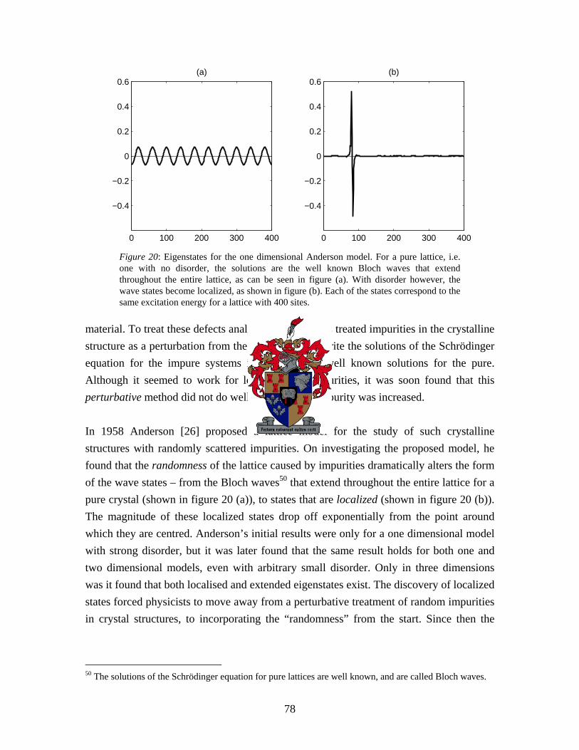
0 100 200 300 400
−0.4
−0.2
0
0.2
0.4
0.6(a)
0 100 200 300 400
−0.4
−0.2
0
0.2
0.4
0.6(b)
Figure 20: Eigenstates for the one dimensional Anderson model. For a pure lattice, i.e. one with no disorder, the solutions are the well known Bloch waves that extend throughout the entire lattice, as can be seen in figure (a). With disorder however, the wave states become localized, as shown in figure (b). Each of the states correspond to the same excitation energy for a lattice with 400 sites.
material. To treat these defects analytically, physicists treated impurities in the crystalline structure as a perturbation from the ideal, trying to write the solutions of the Schrödinger equation for the impure systems in terms of the well known solutions for the pure. Although it seemed to work for low levels of impurities, it was soon found that this perturbative method did not do well if the level of impurity was increased. In 1958 Anderson [26] proposed a lattice model for the study of such crystalline structures with randomly scattered impurities. On investigating the proposed model, he found that the randomness of the lattice caused by impurities dramatically alters the form of the wave states – from the Bloch waves50 that extend throughout the entire lattice for a pure crystal (shown in figure 20 (a)), to states that are localized (shown in figure 20 (b)). The magnitude of these localized states drop off exponentially from the point around which they are centred. Anderson’s initial results were only for a one dimensional model with strong disorder, but it was later found that the same result holds for both one and two dimensional models, even with arbitrary small disorder. Only in three dimensions was it found that both localised and extended eigenstates exist. The discovery of localized states forced physicists to move away from a perturbative treatment of random impurities in crystal structures, to incorporating the “randomness” from the start. Since then the
50 The solutions of the Schrödinger equation for pure lattices are well known, and are called Bloch waves.
78

theory of localization has been studied in much detail, and for a review article on the subject one may consider [27].
5.1.1 The Anderson model in general In general the Anderson model is as follows: suppose that there are a number of sites where, let’s say, an electron can find itself, designated by the index µ . At each of these sites there is a potential well of depth µε , and the probability of an electron hopping from site µ to another site designated by ν is given by the hopping amplitude Vµν . This leads to the following Hamiltonian:
H Vµ µνµ µ ν
ε µ µ ν µ≠
= +∑ ∑ . (5.1)
Here the basis has been chosen in such a way that the state µ represents an electron that finds itself at site µ 51. One is now free to choose the parameters µε and Vµν to sim late a wide variety of physical systems, and to simulate “randomness”, the parameters can be chosen from some probability distribution.
u
As an example, consider the one dimensional Anderson model used to create figure 20. Here the lattice sites have been chosen to lie consecutively on a straight line equidistant from each other, and furthermore, an electron is only allowed to hop between nearest neighbours, the hopping amplitude constant for all of the allowed hops. This is done by choosing the hopping amplitudes as follows:
1, 1
0, 1Vµν
µ ν
µ ν
⎧ − =⎪= ⎨− ≠⎪⎩
, (5.2)
and is so for both figures 20(a) and (b). The choice of the hopping amplitude as 1 for allowed hops is arbitrary, but one that is done often in the literature to set the energy scale. The difference in figures 20 (a) and (b) lie in the choice of the potential well depths
µε . For figure 20 (a) they are all simply equal to 0, i.e.
0µε = (5.3)
for all µ . With this choice of parameters, the solutions of the Schrödinger equation are merely the familiar Bloch waves. For figure 20 (b) however, the potential well depths at 51 Technically these states are called Wannier states, but we shall not go into it here.
79

each of the sites are chosen from a uniform distribution over the interval , the probability density for the potential well depths therefore given by
( )/ 2, / 2W W−
( )( )
1, / 2, / 2( )
0, / 2, / 2
W W
W W
ερ ε
ε
∈ −⎧⎪= ⎨∉ −⎪⎩
. (5.4)
Here the parameter W is used to vary the degree of “disorder” of the system. As a matter of interest, for figure 20 (b) the value of 2.4W = was chosen. It is natural to cast the Hamiltonian given by equation (5.1) in the form of a matrix, the potential well depths µε being the diagonal elements, and the hopping amplitudes Vµν the off-diagonal ones. Even though the choice of µε and Vµν as given by equations (5.2) and (5.4), result in a Hamiltonian matrix that bears little resemblance to the matrices from any of the Gaussian ensembles, it is still, in essence a Random Matrix model. With the off-diagonal elements fixed, each different set of diagonal elements from the probability density given by equation (5.4) results in a different matrix in a new ensemble of matrices. Notably, the symmetry of the matrices in this new ensemble is the same as that of matrices from the GOE.
5.1.2 The Anderson model in two dimensions Let us extend the model discussed in the previous section to two dimensions. Instead of having all the sites lie in a straight line, consider a square lattice of sites lying in the xy plane, equidistant from each other, as depicted in figure 21. Each of these sites are labelled by coordinates i and in the and directions respectively. Once again the j x yprobability density of the potential well depths at each of the sites will be given by equation (5.4), and once again only nearest neighbour hops will be allowed, this time in vertical and horizontal directions. Writing down the Hamiltonian for this model in matrix form can be tricky, therefore let us instead consider an example. For the 4 lattice, as shown in figure 21, the broad form of the Hamiltonian matrix is as follows:
4×
†
†1
†2
†3
4
00
00
A
A
D AA D A
HA D A
A D
⎡ ⎤⎢ ⎥⎢ ⎥=⎢ ⎥⎢ ⎥⎢ ⎥⎣ ⎦
, (5.5)
80

3
2 i
4
1
y1 2 3 4j
x
Figure 21: A square lattice for the two dimensional Anderson model. Each dot represents a site on the xy plane, and are labelled by coordinates ( , ). i j
with the matrices jD and A each a 4 4× matrix. The Hamiltonian is therefore a matrix. To explain, let us consider each column of the two dimensional
lattice in figure 21 as a one dimensional lattice. For such a one dimensional lattice with 4 sites, the Hamiltonian is given by
H2 24 4 16 16× = ×
1
2
3
4
1
1
1 01 10 1 1
0 1
j
jj
j
j
D
εε
ε0
ε
⎡ ⎤⎢ ⎥⎢ ⎥=⎢ ⎥⎢ ⎥⎢ ⎥⎣ ⎦
, (5.6)
with the diagonal elements ijε taken from the probability density given by equation (5.4), and the 1’s on the first super and sub-diagonals representing the hopping amplitudes for upward or downward jumps respectively. The smaller 1’s in the corners are there for enforcing periodic boundary conditions if one would so choose. As for the matrix A , for now it is simply
1 0 0 00 1 0 00 0 1 00 0 0 1
A
⎡ ⎤⎢ ⎥⎢ ⎥=⎢ ⎥⎢ ⎥⎣ ⎦
, (5.7)
81

Figure 22: The same two dimensional lattice as shown in figure 21. This time however, there is a magnetic field perpendicular to the B xy plane – in the z direction. Were an electron starting out at position (2, 2) “hop” along the closed path indicated, it would pick up a phase shift proportional to the magnetic flux φ through the enclosed loop.
the identity matrix. These matrices, when placed in the Hamiltonian as given by equation (5.5), represent the hopping amplitudes for jumps to the right, and the matrices
4 4×
†A the jumps to the left. As A is the identity matrix, it seems a bit redundant to also use †A in equation (5.5). The use of this, however, will become clear a bit later on. Just as
the smaller 1’s in the corners of the matrices jD represent the matrix elements needed for periodic boundary conditions, so too do the “smaller” matrices A and †A in the corners of . H The Hamiltonian matrix for the two dimensional Anderson model given by equations (5.5), (5.6) and (5.7) is symmetrical, and therefore represents a system with conserved time reversal symmetry. It was however mentioned in chapter three that the time reversal symmetry of a system (of charged particles) can be broken by the application of an external magnetic field, and as we shall see, including the effects of a magnetic field in the two dimensional Anderson model leads to a Hamiltonian matrix that is, as expected, Hermitian.
5.1.3 The 2D Anderson model in an external magnetic field The addition of an external magnetic field to the two dimensional Anderson model relies on a physical phenomenon known as the Aharonov-Bohm effect. Briefly, it states that the
3
2 i
4
1
y1 2 3 4
a
φ
( )i λ−1 e
( )i λ2 e
B
j
x
82

wave state of an electron that travels a closed path in an magnetic field will have a shift in phase that is proportional to the magnetic flux through the surface enclosed by the path. To be a little more precise, the multiplication factor due to the phase shift is given by
02 ( / )if e π φ φ= , (5.8)
with φ denoting the magnetic flux. The constant 0φ is equal to ehc , with e the charge of
the speed of light and
is t efore perpendicular
the plane in which the lattice lies, the magnetic flux though the loop indicated in figure
the electron, c h Heisenberg’s constant. Let us suppose that the distance between two sites in the lattice a , as shown in figure 22. With a magnetic field of magnitude B in the z direction, and herto22 is given by
2Baφ = . (5.9)
The magnetic flux through a closed loop is however also given by the contour integral of the magnetic vector potential along the closed loop. The magnetic vector potential is a ector field for which holds
Av
= ∇×B A . (5.10)
The vector potential corresponding to a specified magnetic field is not unique. In the Landau gauge, the vector potential for a uniform magnetic field in the direction is
z
Bx=A y , (5.11)
with y denoting the unit vector in the y direction. Getting back to the magnetic flux, for the enclosed loop shown in figure 22 the flux is equal to the sum of along each of the our ops” in the loop. As the vector ential i
(2 2
Af s in the y direction, the vertical hops, up “h potform , 3) to (1, 3) and down from (1, ) to (2, 2) do not contribute. The horizontal hops however do: as shown in figure 22, for the hop left from (2, 2) to (2, 3) the contribution is
2(2 ) 2Aa aB a Ba= = , (5.12)
and for the hop to the right from (1, 3) to (1, 2) the contribution is
2(1 )Aa aB a B− = − = − a . (5.13)
83

N direction as the vector potential, ote that, due to the fact that this hop is in the opposite
2
the contribution is negative. Adding (5.12) and (5.13) up, we have for the flux through the enclosed loop
2 22Ba Ba Baφ = − = , (5.14)
hich is the same result as that given by equation (5.9).
fter all of this, we can finally get back to the Anderson model. The general form of the
w AHamiltonian for the Anderson model in an external magnetic field remains the same as the form given by equation (5.5). Furthermore, as the magnetic vector potential is in the vertical direction, the hopping amplitudes for up and down hops are not altered, and therefore the matrices jD equation (5.5) remain the same, as given by (5.6). The matrix A , dealing with horizontal hops, does however change. For a 4 4× lattice in an external
gnetic field, the matrix ma A now becomes
( ) 0ie λ
0 00 0 00 0 00 0 0
i
i
i
eA
ee
λ
λ
λ
⎡( )
( )
(4 )
⎤⎢ ⎥⎢ ⎥=⎢ ⎥⎢ ⎥⎣ ⎦
2
3, (5.15)
with
1
2
0 0
2 2Baπ πφλφ φ
= = . (5.16)
In equation (5.5) the hopping amplitudes for hops to the right are given by A , whereas for hops to the left they are given by †A . For an electron somewhere in, say, the second row, a hop to the right will cause its state to be multiplied by a phase factor of (2 )ie λ , effectively changing its phase by 2λ . A hop to the left, however, will cause its state to be multiplied by a phase factor of ( 2 )ie λ− , changing its phase in the opposite direction by
2λ− . With A now given by equation (5.15), the Hamiltonian of the two dimensional rson mo el given by equation (5.5) is no longer symmetrical, as was the case
without an external magnetic field, but Hermitian.
Ande d
84

5.1.4 Numerical experiments As mentioned before, the matrices for the two dimensional Anderson model are not at all like those from the Gaussian ensemble. They do, however, share the same symmetries. Without an external magnetic field, the Hamiltonian matrix for the 2D Anderson model is symmetrical, just as the matrices from the GOE. The application of an external magnetic, however, is expected to break time reversal symmetry, resulting in a Hamiltonian matrix that is not symmetrical, but Hermitian. For the Hamiltonian of the 2D Anderson model in an external magnetic field this is indeed so, as it is for matrices from the GUE. For the purpose of numerical experimentation, a lattice of size 30 30× was considered, resulting in Hamiltonian matrices of size 900 900× . Four different values for λ were considered, and throughout, the disorder was kept constant with the choice of 2.4W = . For each of the four choices of λ , 200 matrices with different realizations of diagonal disorder, from the probability density given by equation (5.4), were diagonalized, resulting in 200 different eigenvalue sequences to be averaged over for each of the four choices. Summed up, the parameters for the four cases investigated are:
W λ
(a) 2.4 0(b) 2.4 ( 0.01/ 30) 2π− ×
(c) 2.4 ( 0.018 / 30) 2π− ×
(d) 2.4 ( 1/ 30) 2π− ×Table 1
The MATLAB code for the generation of Hamiltonian matrices for the two dimensional Anderson model in an arbitrary external magnetic field, as well as a few remarks on the numerical calculations, is given in Appendix C. The idea for these experiments stems from an article by Uski et al. [28]. The results obtained here are in good agreement therewith, and may even surpass it in accuracy due to the (to our knowledge) new unfolding procedure proposed in the following section.
85

−5 0 50
200
400
600
800
(a)
−5 0 50
200
400
600
800
(d)
Figure 23: The cumulative distribution functions for cases (a) and (d) given in Table 1 above. Even though for (d) the external magnetic field is the strongest of the four cases, the cumulative distribution function of the resulting eigenvalue sequence is still essentially the same as for (a), where there is no external magnetic field.
5.1.4.1 The density of states and the unfolding procedure Figure 23 shows the cumulative distribution functions (as given by equation (2.7)) for typical eigenvalue sequences resulting from parameter choices (a) and (d). Whereas for (a) the there is no external magnetic field, for (d) the magnetic field is the strongest of the four cases considered. Still, the corresponding cumulative distribution function, which is a global property of a level sequence, seems virtually identical for both cases. The difference between the eigenvalue sequences therefore have to lie in their local properties, and this is indeed the case as we shall see further on. As a matter of interest, the actual density of states will be briefly considered in Appendix D. Before investigating the local properties of an eigenvalue sequence however, the sequence first has to be unfolded in accordance with the procedure outlined in section 2.3. Briefly, let us go though it once more. The a cumulative distribution function, or step function, of the eigenvalue sequence is given by (equation (2.7)) 1 2 3{ , , , }E E E …
( ) ( ') 'E
n E E dEρ= ∫−∞
, (5.17)
with the discrete level density function ( )Eρ here given by
( ) ( )ii
E E Eρ δ= −∑ . (5.18)
86

If one now had the continuous average cumulative distribution function ( )n E , the unfolded level sequence would simply be given by 1 2 3{ , , , }x x x …
( )i ix n E= (5.19)
for each level iE in the original sequence. As mentioned earlier, the unfolding procedure is not always easy to do in practice – the problem being that one usually does not have ( )n E . If it is not known exactly from theory, then one has to approximate it form experimental data. This is usually done by numerically fitting some sort of line – a polynomial of some order, for instance – to the cumulative density function, or some part there of. Exactly how this fit is done, is the tricky part, as too good a fit will interfere with the local properties of the sequence that we were after in the first place. If the experimental data is however of a certain a nature, a good approximation of ( )n E can be made. Suppose that one has a set of different eigenvalue sequences {N }iE , each corresponding to the same type of system, but with different realizations of disorder. The average cumulative distribution function , averaged over the cumulative distribution functions corresponding to each of the eigenvalue sequences {
( )avn E N( )in E }iE , is
given by
1( ) ( )av ii
n E n EN
= ∑ . (5.20)
Note that is still a step function. To approximate the continuous average distribution function
( )avn E( )n E , one can now, instead of fitting some line to each , one
can interpolate . Even though it is not often that experimental data will be of such a nature that this novel unfolding procedure is applicable, it does in this case lead to very good results, enabling one to investigate the level sequence statistics of the Anderson model in more detail than otherwise possible. An example of this is the average level density briefly discussed in Appendix D.
( )in E( )avn E
As mentioned earlier, for each of the four different choices of magnetic field strength, 200 corresponding Anderson Hamiltonians with different realizations of disorder were diagonalized, resulting in eigenvalue sequences for each case. For each of the four sets of eigenvalues, the continuous average distribution function
200N =( )n E was
87

Figure 24: The NNS distributions for four different external magnetic field strengths, the letters (a), (b), (c) and (d) corresponding to the magnetic field strengths given in Table 1 above. The solid line denotes the approximate NNS distribution of the GOE, given by the Wigner surmise. In the same way, the dashed line approximates the NNS distribution of the GUE. With the magnetic field turned off in (a), the NNS histogram for the eigenvalues of the Anderson model Hamiltonian follow that predicted for the GOE. As the magnetic field’s strength is increased however, moving from (b) to (c), the NNS histograms quickly move away from the GOE to the GUE NNS distribution. For the fourth magnetic field strength (d), the transition from GOE to GUE statistics already seems to be complete.
0 0.5 1 1.5 2 2.5 3 3.50
0.2
0.4
0.6
0.8
1(a)
0 0.5 1 1.5 2 2.5 3 3.50
0.2
0.4
0.6
0.8
1(b)
0 0.5 1 1.5 2 2.5 3 3.50
0.2
0.4
0.6
0.8
1(c)
0 0.5 1 1.5 2 2.5 3 3.50
0.2
0.4
0.6
0.8
1(d)
GOE
GUE
approximated by cubic spline interpolation of the corresponding function , which was then used in equation (5.19) to unfold the relevant level sequences.
( )avn E
5.1.4.2 Local statistics Even though the form of the 2D Anderson model Hamiltonians differ greatly from the matrices in either the GOE or GUE, they do share the same symmetries. Without an
88

Figure 25: The statistic for eigenvalue sequences of the Hamiltonians corresponding to the 2D Anderson model with four different magnetic field strengths. The field strengths are given in Table 1 above, and once again the labels of the four sets of data correspond to the labels used there. The solid line shows the
3∆
3∆ statistic for the GOE, and the dashed line that of the GUE. With zero magnetic field (a), and the magnetic field already turned on (d), the experimental data fits the analytic results for the GOE and GUE exceptionally well. For the weak magnetic fields (b) and (c), the 3∆ statistics lie somewhere in between, indicating that the full transition from GOE to GUE statistics has not yet fully taken place.
0 1 2 3 4 5 6 7 8 9 100
0.05
0.1
0.15
0.2
0.25
(a)
(b)
(c)
(d)
GOE
GUE
external magnetic field, the Hamiltonians for the 2D Anderson model are symmetric, and therefore, just as matrices from the GOE, describe a system with conserved time reversal symmetry. In the presence of a magnetic field, however, time reversal symmetry is broken, and as expected the Hamiltonians for the 2D Anderson model in an external magnetic field are Hermitian – just as the matrices from the GUE. If one were to start out with a system with time reversal symmetry, and then slowly turn on an external magnetic, the question arises of just how the time reversal symmetry is broken. By simulating the gradual increase of an external magnetic field with the 2D Anderson model, it turns out that time reversal symmetry is not broken suddenly, but rather continuously. Figure 24 shows NNS histograms of eigenvalue sequences from the Anderson model Hamiltonians obtained for four different magnetic field strengths, the figure labels corresponding to the labels in Table 1 above. The approximate NNS distributions for GOE and GUE, given by
89

equations (4.29) and (4.30), are shown by the solid and dashed lines respectively. For (a) the magnetic field is zero, and therefore the NNS histogram follows the NNS distribution of the GOE. As the magnetic field is increased to (b) and then to (c), the NNS histograms shift away from the GOE NNS distribution, and closer to the GUE NNS distribution. By now turning the magnetic field up to (d), the transition to GUE statistics seems complete. Note that, although magnetic field (d) is much greater than (b) and (c), it is still relatively small. The transition from GOE to GUE statistics, and therefore the breaking of time reversal symmetry, although not sudden, occurs quite rapidly. To further investigate the local statistics of eigenvalue sequences for the 2D Anderson model Hamiltonians, the statistics for each of the four magnetic field strengths have also been calculated, and are shown in Figure 25. Once again the labels correspond to those in Table 1 above, and once again the analytic results for the GOE and GUE are shown by the solid and dashed lines respectively. With a zero magnetic field for (a), and with the magnetic field already turned on for (d), the
3∆
3∆ statistics match the theoretical results for the Gaussian ensembles almost perfectly. For the weak magnetic fields (b) and (c) however, the statistics lie somewhere in between, indicating that the transition from GOE to GUE statistics, and therefore from conserved to broken time reversal symmetry, has not fully taken place.
3∆
Putting the question of how time reversal symmetry is broken aside, the fact that local statistics of eigenvalue sequences corresponding to the Hamiltonian matrices of the 2D Anderson model fit the level statistics of the GOE and GUE so well, is really quite remarkable. This is especially so, considering the difference in structure between the Anderson model Hamiltonian matrices and the matrices from the Gaussian ensembles. Because of its importance, however, we will again mention that even though there are great differences between them, the Anderson model Hamiltonian matrices do have the same symmetries as the two relevant Gaussian ensembles, alluding to the thought that it is not the distribution of the matrix elements that determine the local properties of the eigenvalue sequence of a random matrix, but its overall symmetry.
90

5.2 More Applications
5.2.1 Nuclear Physics As mentioned before, the field of nuclear physics is where RMT had its inception. This is also the field in which experimental data first became detailed enough for statistically significant tests of the predictions of RMT, culminating in the famous Nuclear Data Ensemble of energy levels of a broad spectrum of nuclei. As an example of its application in this field, figure 7 shows a histogram of the nearest neighbour spacings for energy levels of heavy nuclei taken from the Nuclear Data Ensemble, compared to the NNS distribution predicted by RMT from the Gaussian Orthogonal Ensemble. Figure 26, taken from [29], again shows a comparison between the level statistics of the Nuclear Data Ensemble, and that predicted by RMT, but this time for the statistic. As can be seen, the statistic of the NDE agrees very well with the statistic for the GOE. For comparison, the statistics for the Poisson distribution and the GUE have also been plotted.
3∆
3∆ 3∆
3∆
Figure 27 shows a much older comparison between nuclear energy level data done by Porter and Rosenzweig in 1960 [30]. Figures 27 (a), (b) and (c) show NNS histograms of a number of nuclear energy level sequences, each individual level sequence properly unfolded and containing only levels with the same “good” quantum numbers, and corresponding to odd eigenfunctions. For each of the three graphs, the level sequences were grouped according to the size of their nuclei: (a) the smallest, (b) intermediate and (c) the largest. In (a), where the smaller nuclei are considered, the NNS histogram of their energy levels are much nearer the Poisson distribution than the NNS distribution of the GOE. As the sizes of the nuclei increase however, the NNS histogram approaches the GOE NNS distribution, as can be seen from the progressively better fit as one goes from (b) to (c). Clearly, there seems to be a dependency of the applicability of RMT on the complexity of a system. This is however not the case, as we shall see in the following section.
91

Figure 26: The statistic for level sequences of heavy nuclei taken from the Nuclear Data Ensemble, compared to the
3∆3∆ statistic for the GOE. For comparison, the
statistics for the Poisson distribution and the GUE have also been plotted. As it was for the NNS distribution in figure 7, the correlation between theory and experiment is
3∆
remarkable. Taken from [29].
Figure 27: Histograms of the nearest neighbour spacings for energy levels of an assortment of atomic nuclei. The three different graphs are for three size groupings of nuclei: (a) being the smallest, (b) intermediate and (c) the largest. As the sizes of the nuclei, and therefore their complexity, increase, the NNS histograms approach the NNS distribution of the GOE. The energy levels considered in each sequence all have the same good quantum numbers, and all correspond to odd eigenfunctions. Taken from [30].
92

5.2.2 Quantum Chaos In 1984, Bohigas, Giannoni and Schmit made their famous conjecture, stating [31]: “Spectra of time-reversal-invariant systems whose classical analogs are K systems show the same fluctuation properties as predicted by GOE (alternative stronger conjectures that cannot be excluded would apply to less chaotic systems, provided that they are ergodic)” – and by doing so connected the study of quantum chaos to that of RMT. Before this connection was made, RMT was thought only to apply to system with a great number of degrees of freedom, such as the multi-particle nuclear systems studied at its inception. Now, however, it was apparent this was not an essential property for a system to exhibit RMT statistics, as chaotic systems with as few as 2 degrees of freedom exhibited the same level statistics. Possibly the most well known classical chaotic systems studied are those of a particle free to move over a flat, frictionless surface, bouncing elastically off the sides that enclose it. Due to an obvious analogy, such systems are often referred to as “billiards”, and depending on the configuration of the “table”, it is possible to construct a system for which motion of the ball is chaotic. Examples of such configurations are the Sinai and Cardioid billiards, and following the Bohigas Giannoni Schmit conjecture, the energy levels of their quantum mechanical counterparts should adhere to GOE statistics. On the other hand, for billiards resulting in regular classical motion, such as one with a circular configuration, it is generally accepted [32] that the energy levels of its quantum mechanical analogy exhibit Poisson statistics. This can clearly be seen in Figure 28, taken from [33], which shows NNS histograms for the quantum mechanical energy levels of two different billiards, on the left for a circular configuration, and on the right for a cardioid configuration. Although Bohigas, Giannoni and Schmit initially studied the Sinai billiard as an example of chaotic motion, their conjecture refers to chaotic motion in general. As another example of chaotic motion, Seligman, Verbaarschot and Zirnbauer studied a Hamiltonian of two interacting particles, with the form [34]:
( )2 21 2 1 1 2 2 12 1 2
1 ( ) ( ) ( )2
H p p V x V x V x xλ= + + + + − , (5.21)
with and denoting the momentum each of the particles, and 1p 2p 1x and 2x their positions. The parameter λ is used to vary the relative strength of the interaction
93

Figure 28: NNS histograms of quantum mechanical energy levels for a particle free to move in a two dimensional infinite square well. For the figure on the left, the configuration of the boundary of the well is circular, whereas for the figure on the right the boundary shape is cardioid. On a circular billiard, the classical ballistic motion of a particle is integrable, and therefore the energy levels of the quantum mechanical equivalent have an NNS distribution that follows the Poisson distribution. For a cardioid billiard, however, the classical motion is chaotic. The equivalent quantum mechanical system in this case has an energy level sequence that obeys GOE statistics, as predicted by the Bohigas Giannoni Schmit conjecture. Taken from [33].
Figure 29: The 3∆ tistic and NNS histograms for the energy levels of a Hamiltonian for two interacting particles, showing the transition between GOE and Poisson statistics. The Hamiltonian was constructed in such a manner that the corresponding classical motion could be varied from regular to chaotic by varying the coupling strength between the two particles. Taken from [
sta
34].
94

potential, in effect determining to which extent the motion of the two particles are coupled. With λ set to zero, the motion of the particles would be uncoupled, resulting in motion that is integrable. The potentials functions V all have the general form of
2 4( )V x x x x6α β γ= + + , (5.22)
the parameters α , β and γ free to be chosen independently for each of the three potential functions. With λ set to 1, they found that an appropriate choice of parameters led to motion that was non-integrable, i.e. chaotic. The 3∆ statistic and the NNS distribution of the resulting sequence of energy levels are shown by the top row of figure 29, clearly in correspondence with the GOE results over which they were superimposed. By now decreasing the coupling strength, they found that the statistics of the resulting eigenvalue sequences reverted to Poisson statistics, as can be seen as one moves down from (a) to (e) in figure 29. For (d) and (e), the 3∆ statistic and the NNS distribution for the uniform distribution, i.e. the Poisson distribution, have been superimposed. Even though in (e) the correspondence between the theoretical and “experimental” 3∆ statistics is not very good (for reasons explained in [34]), the “experimental” NNS distribution does match the Poisson distribution with λ set to 0.
5.2.3 Acoustic resonances Physical systems that exhibit some sort of resonance frequencies are certainly a well known appearance. Systems such as a guitar string in one dimension, or the membrane of a drum in two dimensions, are only able to vibrate at certain frequencies, each frequency corresponding to a specific mode of vibration. The resonance frequencies depend on the material of the vibrating media, as well is the system’s geometry. For a drum, for instance, the allowed modes of vibration depend on the material of the membrane, as well as the shape of the drum. The set of resonance frequencies for a square drum would be different to that of a round one. Such a picture of allowed frequencies with corresponding allowed modes of vibration is in many ways analogous to the eigenfunctions and corresponding eigenvalues in quantum mechanics. As it turns out, just as for the energy levels of certain quantum mechanical systems, the resonances frequencies of certain classical systems can be described by Random Matrix Theory.
95

As an example in the previous section on quantum chaos, simple two dimensional systems were discussed who’s eigenvalue sequences are described by RMT. In analogy to these billiard systems, consider thin vibrating plates with similar geometries. Here, in principle, the local statistics of the allowed vibrational modes of a plate do not depend on the internal structure of the material, rather on its overall geometry. In [35] the vibrational modes of a large number of such plates were studied, and the results compared to that of RMT. For a round plate, for instance, it was found that the sequence of resonance frequencies had an NNS distribution that is well described by the Poisson distribution. However, for a plate shaped as one quarter of a Sinai stadium, as can be seen on the left of Figure 30, this was not the case. As the Sinai stadium configuration would result in a billiard system with chaotic motion, one might expect that the resonance frequencies of the Sinai stadium plate would be well described by GOE statistics. At first glance, however, this does not seem to be the case. This is due to the fact that, for a plate such as this, there are two independent ways in which it can vibrate: called the flexural and extensional modes. Each method of vibration has its own independent set of resonance frequencies, the sequence of resonance frequencies for the plate as a whole being a superposition of these two sub-sequences. As it turns out, for this specific case, there is roughly the same number of frequencies in both of the sub-sequences, distributed over the same frequency interval. As briefly discussed in Appendix B, the statistics of such an overall sequence can be described in terms of the statistics of its constituent sub-sequences. A special case of such a composite sequence, is the superposition of two GOE sequences, each with the same overall level density, or fractional density. This “ensemble” is sometimes referred to as the 2GOE, the NNS distribution of which is shown by the dashed line in figure 30. As the histogram of experimental data matches the NNS distribution of the 2GOE, it would seem that both of the two sub-sequences are indeed described by the GOE. For the graph on the right of figure 30, the same shape of plate was used once again. This time, however, two narrow grooves were made over the surface of the plate, with a depth of half of the plate’s thickness. What these grooves did, was cause the flexural and extensional modes to interact, and with the two sub-sequences no longer independent, as can be seen in the graph on the right of figure 30, the statistics of the resulting sequence of resonances are now described by that of the GOE. Another application of RMT to acoustic resonances was to the vibrational modes of quartz blocks [36]. In contrast to the vibrating plates discussed above, the system
96

Figure 30: On the left hand side we have an NNS histogram for a sequence of resonance frequencies for a thin aluminium plate in the shape of one quarter of a Sinai stadium. For such a plate there are two independent ways of vibrating, called flexural and extensional modes, each with their own sub-sequence of resonance frequencies. The sequence of resonances for the plate can therefore be seen as a superposition of these sub-sequences, the statistics of which can be described in terms of that of its sub-sequences as discussed in Appendix B. For the superposition of two GOE sequences of equal density, some times referred to as 2GOE, the NNS distribution has been plotted as the dashed line. As can be seen, the NNS histogram for the resonance frequencies match it well, alluding to the fact the flexural and extensional sub-sequences are each independently described by the GOE. For the figure on the right, the same shape of plate was used. This time, however, two thin grooves were made across the plate, causing the flexural and extensional modes to interact. The sub-sequences no longer independent, the resulting NNS histogram now follows that of the GOE. Taken from [35].
Figure 31: The 3∆ statistic and NNS histograms for acoustic resonances of a rectangular quartz block. Due to the shape of the block, and its internal crystal structure, the block has a symmetry that allows two independent modes of vibration. With the block still intact, the NNS histogram in (a) therefore follows that of the 2GOE shown by the dashed lines. This symmetry was then gradually broken by removing a successively larger octant of a sphere from one of the block’s corners, resulting in a shift of the NNS histograms toward that of the GOE (shown by the dotted lines), as can be seen in figures (b) through (f). Although the 3∆ statistics devi from the theoretical prediction for large arguments, the match is still good for smaller values. The lower line shows that of the GOE, and the upper that of the 2GOE. Figures (x) show the statistics of he resonance frequencies with a large spherical section removed, the sphere’s centre near one of its corners. The correspondence to GOE statistics is now very
ate
good. Taken from [36].
97
conside rum of allowed vibrational modes now red is now three-dimensional, and the spectstrongly depend on the crystalline structure of the quartz. Even though the configuration of the blocks were regular – the blocks considered were rectangular blocks with dimensions 214 25 40mm× × – the resonance frequencies were not uniformly distributed, the underlying crystal structure of the quartz here playing an important role. As it turns out, with the dimensions and the crystal structure as they were, the quartz blocks displayed a symmetry that allowed for two independent ways of vibration, leading to an NNS distribution well described by the 2GOE; as can be seen in part (a) of figure 31. To investigate the effect of breaking this symmetry on the statistics of the resonance spectrum, successively larger octants of a sphere were removed from one of the block’s corners. As the part removed became larger, the symmetry of the system was gradually broken more and more, resulting in a shift of spectral statistics from that of the 2GOE to that of the GOE. This can be seen as the part removed becomes larger from (b) through (f) in figure 31. For the 3∆ statistics the match of experimental data to the theoretical results from the GOE and 2GOE show large discrepancies for large interval lengths, even though the match is good for smaller arguments. For part (x) in figure 31, as a control, a much larger section of the quartz block was removed as for the preceding experiments. Furthermore, the centre of the spherical section removed did not coincide with where one of the block’s corners was, rather, it was located just inside the original block near one of the corners. With the structure now such that no symmetries remained, and the geometry of the block now such that the classical motion of a particle inside such a shape would be chaotic, the spectral statistics, as can be seen, are well describes by the results from the GOE.
98

6 Closing remarks
Since its inception in the 1950’s, Random Matrix Theory has certainly gone way beyond its intended scope of Nuclear Physics. As seen in the preceding chapters, the predictions of RMT apply to a broad spectrum complex systems, from the financial markets to the zeros of the Riemann ζ function. This truly remarkable spectrum of applications may lead one to the question of why RMT is indeed so successful, and it is to this that we now briefly turn.
6.1 Why does RMT work? One thing that all the systems to which RMT applies have in common, is that in some way or another, each of them give rise to an ordered sequence of numbers, such as the energy levels of a quantum chaotic system, or the resonance frequencies of a quartz block. The predictions of RMT involve the statistical properties of such sequences, derived by averaging over entire ensembles of level sequences corresponding to ensembles of random matrices. Whereas for theory, averaging over an ensemble is normally easier to do, it is usually not possible to do in practice. As is often the case, only a single sequence of experimentally obtained data is available. To obtain statistical information, one then has to average over parts of a single sequence of levels. These two approaches, that of ensembles averaging and averaging over individual level sequences, do not necessarily lead to the same results. For RMT, however, this is assumed to be true, and is called the ergodic hypothesis.52
6.1.1 Universality Specifically, the predictions of RMT are relevant to how, statistically, individual levels in a sequence are positioned relative to one another. These statistics are referred to as the local properties, or sometimes, the fluctuation properties of a sequence. Even though the many systems to which RMT applies give rise to level sequences with vastly different overall distributions, the fluctuation properties of these level sequences seem to be universal. To get a qualitative feel for how the global properties and local properties of a
52 In the context of quantum mechanics this is in analogy to what was said in section 3.1, that the ensemble of matrices be constructed in such a manner that the specific Hamiltonian matrix of the physical system under investigation lie in it, and in a sense, be more probable.
99

Approximating quadratic potential
Local minimum x
V(x)
Figure 32: Instead of the quadratic confining potential shown in figure 8, the confining potential for the system of charged particles is now more general. Even so, the statistical properties of the particle position will, at least around a local minimum, be the same as that of a system with only a quadratic confining potential.
level sequence are independent of each other, we return to the Coulomb gas analogy discussed in section 4.3.
6.1.1.1 The Coulomb gas analogy revisited In section 4.3 an analogy was made between a level sequence from one of the Gaussian ensembles and the positions of charged particles along a straight line, interacting with a Coulomb potential in a two dimensional world. In addition to the interaction potential, the particles were all confined to some region of the line by an additional external potential. Instead of the confining potential being quadratic, given by equation (4.21), consider a more general form, such as the one displayed in figure 32. For the general potential , in a similar way to equation (4.22), the total potential energy of the system is given by
( )V x
1 2 3( , , , ) ( ) logi ji i j
W x x x V x x x<
i= − −∑ ∑… , (6.1)
the ix ’s being the positions of the charged particles. In the same way that a quadratic confining potential corresponds to the Gaussian ensembles, the general confining potential corresponds to an ensemble of matrices with a matrix element j.p.d.f. given by equation (3.42) as
( )V x
Tr( ( ))1( ) V HCH eρ −= . (6.2)
100

Particles repel each other
Figure 33: The electrostatic analogy to Dyson’s circular ensembles, the particles also repel one another with the two dimensional Coulomb potential. Confined to a ring, however, there is no need for a confining potential, resulting in a uniform density.
Even though calculating ensemble averages for such a potential may not be easy, it is possible to approximate them. For a small interval around the local minimum of indicated in figure 32, one can approximate the potential by a quadratic one. Once this is done, the level statistics, at least for the small interval around the local minimum, is simply that of the Gaussian ensembles. The thought now, however, is that it is only the average distribution of levels that depends on the confining potential, i.e. away from the local minimum, the local properties are still those of the Gaussian ensembles, even though the average level density is not.
( )V x
A different example of a electrostatic system that has bearing on RMT, is the one shown by figure 33. Once again the charged particles repel each other with a Coulomb potential in two dimensions. This time, however, the particles are confined to move along a circular loop, embedded in two dimensions. This system is analogous to Dyson’s Circular ensembles, mentioned in section 3.2.4.2. With the particles constrained to a closed domain, a confining potential is no longer needed. Even though there is no confining potential at all, resulting in a constant particle density, the local statistics for the particle positions are still the same as the local properties of the Gaussian ensembles.53
53 Seeing as Wigner’s Gaussian ensembles and Dyson’s Circular ensembles lead to the same local statistics of a level sequence, these predictions are sometimes referred to as Wigner-Dyson statistics in general.
101

6.1.1.2 Geometric Correlations In terms of the Coulomb gas analogy, the independence of the local correlations between particle positions from the confining potential means that they are dependent only on the interaction potential (equation (4.20))
( ) logint i ji j
V x x x<
= − −∑ . (6.3)
With the analogy to an ensemble of random matrices, this means that the local properties of a level sequence from such an ensemble is dependent only on the Jacobian that relates the matrix element space to its equivalent eigenvalue space, and the Jacobian for the change from matrix element space to eigenvalue space is dependent only on the type of similarity transformation allowed on the ensembles (see, for instance, equation (4.8)). As the type of similarity transformation is dependent on the symmetry of the matrices in an ensemble, it therefore stands to reason that the corresponding local level statistics depend solely on the symmetry of an ensemble’s constituent matrices. This dependence of local level statistics solely on the symmetry of the matrices in an ensemble, via the Jacobian relating matrix element to eigenvalue space, is called the hypothesis of geometric correlations [7]. This is a different point of view from the two fundamental hypotheses originally considered by Wigner, that of independently distributed matrix elements, and invariance under basis transformation.
6.1.2 Level repulsion When studying the energy levels of complex atomic nuclei, Wigner proposed that the energy levels repel each other, leading to his famous NNS distribution for nuclear energy levels – the Wigner Surmise. As the energy levels of a single nucleus are certainly fixed, the concept of level repulsion may not be clear. To get a better idea as to what is meant by it, let us once again briefly consider the Anderson model discussed in chapter 5 as an example. Figure 34 shows the positions of energy levels of the two dimensional Anderson model as a function of the strength of the external magnetic field. For the figure on the left the disorder W (see equation (5.4)) has been set to zero, whereas for the figure on the right it has been set to 2.4. With the strength of the magnetic field slowly changing, so too do the positions of the energy levels, tracing out a path in energy space. With no disorder, these
102

Figure 34: The fluctuation of a few energy levels of the two dimensional Anderson Hamiltonian discussed in chapter 5, as the external magnetic field is varied. For the figure on the left, there is no disorder, with set to zero (see equation (5.4)). Clearly the paths of the energy levels cross. For the figure on the left, on the other hand, W has been set to 2.4. With disorder present, the paths of the energy levels behave very differently, not crossing each other once. The levels seem to repel each other, as the charged particles repel each other in the Coulomb gas analogy. The relationship between
W
λ and the strength of the external magnetic field is given by equation (5.16).
paths clearly cross each other, whereas for the case with disorder, they do not. The energy levels seem to avoid each other, just as charged particles would in the Coulomb gas analogy of section 4.3, and it is only systems that exhibit such level repulsion to which RMT applies. It may seem strange that RMT can apply both to complex systems such as heavy atomic nuclei, and simple systems such as the quantum mechanical Sinai billiard. Furthermore, RMT applies to the energy levels of an electron in a crystalline structure with randomly scattered impurities54. The connection between the three, is that in each case the there are no constants of motion except energy, making it impossible for levels to cross. In the context of classical mechanics, such systems are referred to as non-integrable, or chaotic. For each of the three systems, the reason for the system to be chaotic is different. For the first, it is the complexity of the system, for the second it is the random impurities off which the electron scatters, and for the third it is simply the geometry of the two dimensional system. In this context, the Bohigas Giannoni Schmit conjecture may not seem strange at all, rather, be a fundamental requirement for the application of RMT.
54 System such as this can be modelled by an Anderson model.
103

6.2 Conclusion Random Matrix Theory offers a new kind of statistical description of disordered systems. Classically, RMT is concerned with the local statistical properties of eigenvalue sequences from systems that can be written in terms of an eigenvalue equation. Even the complex part of the zeros of the Riemann ζ function are thought to be the eigenvalues of some Hermitian operator. Since its inception in the field of Nuclear Physics, this description has found to apply to a broad spectrum of seemingly unrelated systems, such as the acoustic resonances of a quartz crystal, or the statistical description of the eigenvalues of a quantum chaotic system. Even though the level sequences that arise from these different physical systems have markedly different overall distributions, the fluctuation properties that they exhibit seem to be universal. Even within a certain field of study, the universality of level fluctuations seem may seem strange. Why, for instance, should the energy levels of two different heavy nuclei display the same fluctuation properties? Although not fully understood, this certainly does seem to be the case. As with any statistical description, detailed information of a system is lost. Random Matrix Theory can certainly not predict exactly where the energy levels of some heavy nuclei will lie. As is the case with classical statistical mechanics, RMT however offers new information that may not have been apparent without a statistical description. The use of classical RMT lies in the fact that the fluctuation properties of a system’s corresponding eigenvalue sequence are independent of its detailed structure. Rather, the fluctuation properties of such an eigenvalue sequence depend solely on the systems overall symmetries. As we have seen in chapter 5, RMT can therefore be used to gain insight into the symmetry properties of a system by studying the statistical properties of its corresponding eigenvalue sequence. Furthermore, this allows one to use RMT as a classification tool, grouping vastly different systems into symmetry classes on account of the level fluctuation properties that they exhibit. As a matter of fact, there are as many as ten different universality classes that have been studied in various fields, all of them able to be classified in terms of symmetric spaces [37]. Three of the these classes correspond to the Gaussian ensembles discussed in this thesis. Briefly, the rest of them correspond to the three chiral ensembles, introduced in the field of QCD, and the four Altland-Zirnbauer ensembles, used in the field of super conductance. Since its inception in the 1950’s RMT has grown tremendously in scope, and has even become a field of study in its own right. With this growth, the mathematical tools
104

developed have allowed ensembles of random matrices to model an ever increasing variety of systems, from the fluctuations of economic markets, to a statistical description of conductance in mesoscopic systems. With applications to “new” physics, such as quantum gravity [38] and QCD [39], concepts of Random Matrix Theory have even been applied to M-Theory [40], in the search for the Theory of Everything.
105

Appendix A The exact average level density of the GUE As an interesting note, the exact level density for the size dependent GUE (as derived in [9]) is written in terms of the eigenfunctions of the quantum mechanical harmonic oscillator. These eigenfunctions, or oscillator wave functions, are given by
2
21 2
1( ) ( )(2 ! )
x
j jjx e H x
jϕ
π−
= ,
with the ’th Hermite polynomial given by ( )jH x j
[ ]
2 2/ 2 2
0
(2 )! ( 1)!( 2 )!
j j j ix x i
ji
d xH e e jdx i j i
−−
=
⎛ ⎞= − = −⎜ ⎟ −⎝ ⎠∑ .
The exact level density for the size dependent GUE with constituent matrices of size is then given by N N×
1
2( ) ( )N
N i0i
x xσ ϕ−
=
=∑ ,
and is shown, normalised, for 20N = in figure 35 together with Wigner’s semi-circle law.
Figure 35: The exact average level density for the size dependent GUE with constituent matrices of size withN N× 20N = . For comparison, Wigner’s semi-circle law for
is also shown. The distributions have been normalized in the same way. N → ∞
106

AppeSuperpositio
we have a level sequence with (constant) density
ndix B n of independent spectra
ρLet us suppose that , composed by the mber of sequences, each with (constant) density superposition of a nu iρ . Then we have
ii
ρ ρ=∑ .
For the fractional density of each of the level sequences, given by
iif
ρρ
= ,
we therefore have
1ii
f =∑ .
The statistical properties of a level sequence composed by the superposition of a set of dependent level sequences can be expressed in rms of the statistical properties of each
individual sequence. Let us start with the NNS distribution. Suppose the ’th component in te
ilevel sequence has a NNS distribution ( )ip x . By then defining for each of the component level sequences the functions ( )i xψ as
( ( )x
i ix)0
p y dyψ = ∫and
( )iE x as
( )0 0
( ) 1 ( ) ( )i i ixE x y dy p x y z dydzψ
∞ ∞ ∞= − = + +∫ ∫ ∫ ,
we have for the NNS distribution of the mixed level sequence [9]
2 22 ( ) 1 ( ) 1 ( )( ) ( )
( ) ( )i i i i
i i ii i ii i i i i
P x E x f fE f x E f x
⎢ ⎜= + −⎜ ⎟ ⎜ ⎟⎢ ⎥ ⎜ ( )i i
ii i
p f x f x f xfE f x
ψ ψ⎡ ⎤⎛ ⎞⎛ ⎞ ⎛ ⎞ ⎛ ⎞− −⎡ ⎤ ⎥⎟⎜ ⎟ ⎟⎢ ⎥
⎣ ⎦ ⎝ ⎠ ⎝ ⎠⎣ ⎦⎝ ⎠ ⎝ ⎠∑ ∑ .
s an example, a superposition of independent level sequences, found in the literature, is sequences from the GOE with equal fractional densities.
Approximating the NNS distributions of these sequences with the Wigner surmise, we
∑∏
Aa superposition of two level
have for the NNS distribution of the mixed sequence
107

Figure 36: The NNS distribution of the 2GOE, obtained by the superposition of two independent level sequences from the GOE. The solid line gives an approximation of the NNS distribution for the 2GOE, and for comparison the dashed line show the Wigner surmise.
( )212 2 2
1( ) ( ) ( ) 1 ( )2
x x xwP x E p ψ⎡ ⎤= + −⎣ ⎦ ,
e Wigner surmise given by equation (4.29), and the functions ( )1( )wp xwith th and xψ( )E x by
2
224 2( ) and ( ) 1
xx x
0x e E x e dx
π πψ
π− −=1− = − ∫ .
Such a superposition of two independent GOE level sequences result in a new ensemble of level sequences sometimes referred to as the 2GOE, and its approximate NNS istribution, given above is shown, in figure 36.
d
As a matter of interest, the number variance and the 3∆ statistic for a sequence obtained by the superposition of independent level sequences, each with number variance ( )ViN L and 3∆ statistic 3 ( )i L∆ , are given by
3 3( ) ( ) and ( ( )V Vi i i ii i
N L N f L L f L= ∆ = ∆∑ ∑ .
)
108

Appendix C On the calculation of the eigenvalues for the 2D Anderson Hamiltonian
r the section on the Anderson model in Chapter 5, numerical calculations were done in ATLAB. The function used for setting up a 2D Anderson Hamiltonian for an arbitrary
grid size, disorder and external magnetic field, is as follows:
function H=buildandersonfinal(n, L, W, lambda, flag) %constructs the hamiltonian matrix for the 2 dimensional anderson / tight %binding model for a strip in an external uniform magnetic field perpendicular to the %lattice, using the landau gauge. For simplicity the nearest neighbour %hopping amplitude is equal to one. % % H=buildandersonfinal(n, L, W, lambda, flag) %H returns the hamilotnian matrix (sparse) %n, L is the size of the lattice (nxL), L being the number of columns %W is the measure of the diagonal disorder (uniformly distributed in an interval of W % around 0) %lambda gives the strength of the external magnetic field %flag flag ~= 0 means periodic boundry conditions are used N=n*L; %construct the diagonals disorder=(rand(N,1)-.5)*W; hopright=repmat((exp(i*(1:n)*lambda)'), L, 1); hopleft=repmat((exp(-i*(1:n)*lambda)'), L, 1); justhop=ones(N,1); %put them all together H=spdiags([hopright, justhop, disorder, justhop, hopleft], [n, -1, 0, 1, -n], N, N); %remove a few unwanted elements for j=1:(n-1) m=n*j; H(m+1, m)=0; H(m, m+1)=0; end %periodic boundry conditions if flag~=0 H=H + spdiags([hopleft, hopright], [(N-n), -(N-n)], N, N); %up and down periodic boundry conditions for j=1:n H(j*n, (j-1)*n+1)=1; H((j-1)*n+1, j*n)=1; end end
For the numerical experiments in chapter 5, periodic boundary conditions were not used. It is however possible to do, by setting the parameter flag not equal to zero in the function
FoM
109

above. With periodic boundary conditions, the values of λ (related to the magnetic field id of strength by equation (5.16)) are restricted due to continuity considerations. For a gr
size N N× , the allowed values are
2 nNπλ = ,
for a In ch es, one quickly runs into ms. The fi the high computational complexity of the problem. Con , it was found that the computational time as
If one were to consider a grid of size
ny integer n .
apter 5, a grid size of 30 30× was considered. For larger grid sizproble rst is due to
sider a d of size N N× . As N gets largergri T incre es as
6~ ( )T O N .
2 2N N× , for instance, the computational time would increase by a factor of 462 6= . A second problem is the memory required to store the A atrix. As an N N×nderson Hamiltonian m grid results in a Hamiltonian matrix of dime matrix for a nsions N N× , the size of a Hamiltonian2 2 2 2N N× grid would increase by a With iltonians by “brute force”, using MATLAB’s eig() function. For a larger grid sizes, it is possible, first of al t of matrix indices and their corresponding values for all non zero elements. As Anderson Hamiltonians are very sparse, this greatly reduces the storage requirements. Secondly, it is possible to compute only a selection of eigenvalues for a specified Hamiltonian matrix. In MATLAB, this can be done using the func uses ARPACK, an implementation of the implicitly restarted Arnoldi method no magnetic field, it has how plementation of the Lanczos algo putationally efficient [42]. These considerations, already important for the two dimensional Anderson model, are much more serious when inve g the Anderson model in three dimensions.
factor of 42 16= .
a grid size of ×30 30 , we were able to diagonalize the Anderson Ham
l, to represent a Hamiltonian matrix as a se
tion eigs() function, which [41]. For the Anderson model with
ever been found that the Cullum and Willoughby imrithm is far more com
stigatin
110

Appendix D The smoothed level density function for the 2D Anderson model As a matter of interest, the average level density of the two dimensional Anderson model is given here. The dashed line in Figure 37 shows the smoothed average level density as a
nction of energy for a lattice with no external magnetic field. The solid line, however, gives the average level density with an external magnetic field present, the field fu 30 30×
strength given by ( 1/ 30) 2λ π= − × , corresponding to case (d) in section 5.1.4.
h es were then smoothed using MATLAB’s cubic spline smoothing function csaps() with the appropriate choice of parameters. Even though the resulting
oothed level density functions are by no m ns exact, they show the qualitative
ions for the two dimensional ed line), and with the external
magnetic field strength given by
The average level densities shown in figure 37 were obtained as follows: firstly, the continuous average cumulative distributions, approximated as in section 5.1.4.1, were differentiated numerically to obtain rough level densities for the two cases. These “roug ” level densiti
sm eabehaviour of the actual functions.
Figure 37: The smoothed average level density functAnderson model with no external magnetic field (dash
( 1/ 30) 2λ π= − ×el density caused
(solid line). The most remarkable feature are the oscillations of the lev by the presence of a magnetic field. With the increase in field strength, it was found that the amplitude of these oscillations increased, as did the distance between consecutive peaks, the oscillations soon covering the entire spectrum.
111

References [1] Wishart J Biometrika 20 32 (1928)
[2] Wigner E P Proc. Cambridge Philos. Soc. 47 790 (1951)
[3] Garg et al. Phys. Rev. 134 B 72)
[4] Dyson F J J. Math. Phys. 3 140 (1962)
[5] Brody et al. Rev. M 981)
985 (19
od. Phys. 53 385 (1
] Guhr et al. Phys. Rep. 299 189 (1998) [6
[7] Beenakker C W J Rev. Mod. Phys. 69 731 (1997)
[8] Eynard B Random Matrices http://www-spht.cea.fr/articles/t01/014/publi.ps.gz (2001)
[9] Mehta M L Random Matrices Academic Press, New York (1991)
[10] Porter C E ed. Statistical Theories of Spectra: Fluctuations Academic Press, New York (1965)
[11] Bohigas O, Giannoni M J Lecture Notes in Physics 209 1 (1984)
[12] Hayes B American Scientist 91 296 (2003)
[13] Dyson F J, Mehta M L J. Math. Phys. 4 701 (1963)
] Andersen A Topics in Random Matrix Theory M.Sc. thesis, Nieils Bohr Institute, University of
Copenh
[15] Pande
[16] Wign ic
Press,
[17] Ballen apore 250
(1998)
[18] Porter C Sci.
Fennicae, Se
[19] Pandey tween
orthog
[20] We
[21] Bohig Riedel,
Dortre
[22] Meht 0 (1960)
[23] Gaudi cl. Phys. 25
447 (
[24] Odl odlyzko
[14
agen (1999)
y A Ann. Phys. 119 170 (1979)
er E P Group theory and its application to quantum mechanics of atomic spectra Academ
New York Chapter 26 (1959)
tine L E Quantum Mechanics: A Modern Development World Scientific Pub Co., Sing
E, Rosenzwieg N Statistical properties of atomic and nuclear spectra Ann. Acad.
rie A VI Physica 44 1 (1960)
A, Mehta M L Gaussian ensembles of random Hermitian matrices intermediate be
onal and unitary ones Commun. Math. Phys. 87 449 (1983)
yl H Classical Groups Princeton University Press, Princeton N.J. (1946)
as O, Haq R U, Pandey A, Böchhoff K H(Ed.) Nuclear Data for Science and Technology
cht 809 (1983)
a M L, Gaudin M On the density of eigenvalues of a random matrix Nucl. Phys. 18 42
n M Sur la loi limite de l’éspacement des valeurs propres d’une matrice aléatoire Nu
1961)
yzko A M http://www.dtc.umn.edu/~
[25] For 36 R1
(200
rester P J, Snaith N C, Verbaarschot J J M Developments in random matrix theory J. Phys. A
3)
112

[26] Anderson P W Absence of diffusion in certain random lattices Physical Review 109 1492 (1958)
rdered electronic systems Reviews of Modern Physics 57 287 (1985)
niversal correlations in the two-dimensional
8 v1 (1998)
ation properties of nuclear energy levels: do theory and
16 (1982)
of energy levels” in complex atomic spectra Physical Review
universality of
er M R Quantum spectra and transition from regular to
15 (1998)
agen (1997)
ygärd J, Oxborrow M Symmetry breaking and spectral statistics
[37 6 (1996)
[39 rschot J J, Wettig T Random Matrix Theory and chiral symmetry in QCD Annu. Rev. Nucl.
[40
lphia (1998)
del of localization: a
[27 ] Lee P A, Ramakrishnan T V Diso
[28] Uski V, Mehlig B, Römer R A, Schreiber M Smoothed u
Anderson model arXiv:cond-mat/981125
[29] Haq R U, Pandey A, Bohigas O Fluctu
experiment agree? Physical Review Letters 48
[30] Rosenzweig N, Porter C E “Repulsion
120 5 (1960)
[31] Bohigas O, Giannoni M J, Schmit C Characterization of chaotic quantum spectra and
level fluctuation laws Physical Review Letters 52 1 (1984)
[32] Berry M V, Tabor M Proc. R. Soc. London Ser A 356 375 (1977)
[33] Bäcker A Ph.D. thesis Universität Ulm (1998)
[34] Seligman T H, Verbaarschot J J M, Zirnbau
chaotic classical motion Physical Review Letters 53 2
[35] Bertelsen P Quantum chaos and vibration of elastic plates M.Sc. thesis, Niels Bohr Institute,
University of Copenh
[36] Ellegaard C, Guhr T, Lindemann K, N
of acoustics resonances in quartz blocks Physical Review Letters 77 4918 (1996)
] Zirnbauer M R, J. Math. Phys. 37 498
[38] Di Francesco P, Ginsparg P, Zinn-Justin J 2-D Gravity and Random Matrices Phys. Rep. 254 1 (1995)
] Verbaa
Part. Sci. 50 343 (2000)
] Bilal A, Fortsch. Phys. 47 5 (1999)
[41] Lehuocq R B, Sorensen D, Yang G ARPACK Users Guide: Solution of Large Scale Eigenvalue
Problems with Implicitly Restarted Arnoldi Methods SIAM, Philade
[42] Elsner U, Mehrmann V, Milde F, Romer R A, Schreiber M The Anderson mo
challenge for modern eigenvalue methods SIAM J. Sci. Comput. 20 2089 (1999)
113