basic coupled oscillator theory applied to the wilberforce ... · pdf filebasic coupled...

Introduction

One Degree of . . .

Two-Degree-of- . . .

Normal Modes

Conclusion

Home Page

Title Page

JJ II

J I

of 16

Go Back

Full Screen

Close

Quit

Basic Coupled Oscillator Theory Applied to the Wilberforce

Pendulum

Misay A. Partnof and Steven C. Richards

May 4, 2004

Abstract

In this article, we outline some important characteristics of coupled oscillators that simplify themath used to set up and solve a system of second order homogeneous coupled differential equationsdescribing the motion of the Wilberforce Pendulum.

1. Introduction

The Wilberforce pendulum is a vertical pendulum, where the mass at the end of a spring can oscillatenot only in the vertical direction, but it can also rotate with oscillatory motion (see Figure 1). Alsothe energy of the system is transferred between the vertical and rotational oscillations. The amplitudeand frequency of vertical oscillations are dependent on the amplitude and frequency of oscillation inthe rotational direction, and visa-versa. Since the Wilberforce pendulum requires two independentcoordinates to describe its motion, it is a two-degree-of-freedom-system.

2. One Degree of Freedom Systems

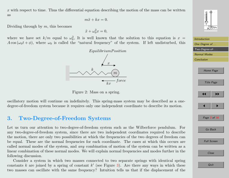
We are all familiar with the mass-spring problem. The pendulum bob with mass m is attached to aspring with spring constant k on a frictionless surface. Given an initial displacement x, the only forceacting on the mass is the restoring force −kx (see Figure 2). By Newton’s second law of motion the forceis equal to a mass times its acceleration, or F = ma = mx = −kx, where x is the second derivative of

Introduction

One Degree of . . .


Normal Modes

Conclusion

Home Page

Title Page

JJ II

J I

of 16

Go Back

Full Screen

Close

Quit

Figure 1: Wilberforce Pendulum.

Introduction

One Degree of . . .


Normal Modes

Conclusion

Home Page

Title Page

JJ II

J I

of 16

Go Back

Full Screen

Close

Quit

x with respect to time. Thus the differential equation describing the motion of the mass can be writtenas

mx + kx = 0.

Dividing through by m, this becomesx + ω2

0x = 0,

where we have set k/m equal to ω20 , It is well known that the solution to this equation is x =

A cos (ω0t + φ), where ω0 is called the “natural frequency” of the system. If left undisturbed, this

km

x

EquilibriumPosition

kxforce

Figure 2: Mass on a spring.

oscillatory motion will continue on indefinitely. This spring-mass system may be described as a one-degree-of-freedom system because it requires only one independent coordinate to describe its motion.

3. Two-Degree-of-Freedom Systems

Let us turn our attention to two-degree-of-freedom system such as the Wilberforce pendulum. Forany two-degree-of-freedom system, since there are two independent coordinates required to describethe motion, there are only two possibilities at which the frequencies of the two degrees of freedom canbe equal. These are the normal frequencies for each coordinate. The cases at which this occurs arecalled normal modes of the system, and any combination of motion of the system can be written as alinear combination of these normal modes. We will explain normal frequencies and modes further in thefollowing discussion.

Consider a system in which two masses connected to two separate springs with identical springconstants k are joined by a spring of constant k′ (see Figure 3). Are there any ways in which thesetwo masses can oscillate with the same frequency? Intuition tells us that if the displacement of the

Introduction

One Degree of . . .


Normal Modes

Conclusion

Home Page

Title Page

JJ II

J I

of 16

Go Back

Full Screen

Close

Quit

k k′ km1 m2

x1 x2

EquilibriumPosition

kx kxforces

Figure 3: Horizontal mass-spring system: equal initial displacement.

k kk′m1 m2

x1 x2

EquilibriumPosition

(k + 2k′)x (k + 2k′)xforces

Figure 4: Horizontal mass-spring system: equal and opposite initial displacement.

masses are exactly equal in direction and magnitude, then the joining spring will remain slack and canbe ignored as both masses (being uncoupled) will oscillate with their natural frequencies

√k/m. If the

displacement of each mass is exactly equal and opposite (see Figure 4), then the force acting on eachmass will be (k + 2k′)x. Setting this equal to F = ma = mx we get the the differential equation

x +(

k′ + k

m

)x = 0.

Then the frequency at which each mass oscillates is√k′ + k

m.

In these two scenarios in which the masses oscillate with the same frequency, they oscillate with the”normal frequencies” of the system. The motion that the masses exhibit when oscillating at these normal

Introduction

One Degree of . . .


Normal Modes

Conclusion

Home Page

Title Page

JJ II

J I

of 16

Go Back

Full Screen

Close

Quit

frequencies are the normal modes of the system. Any possible combination of the motions of the twomasses can be written as a linear combination of these normal modes.

4. Normal Modes

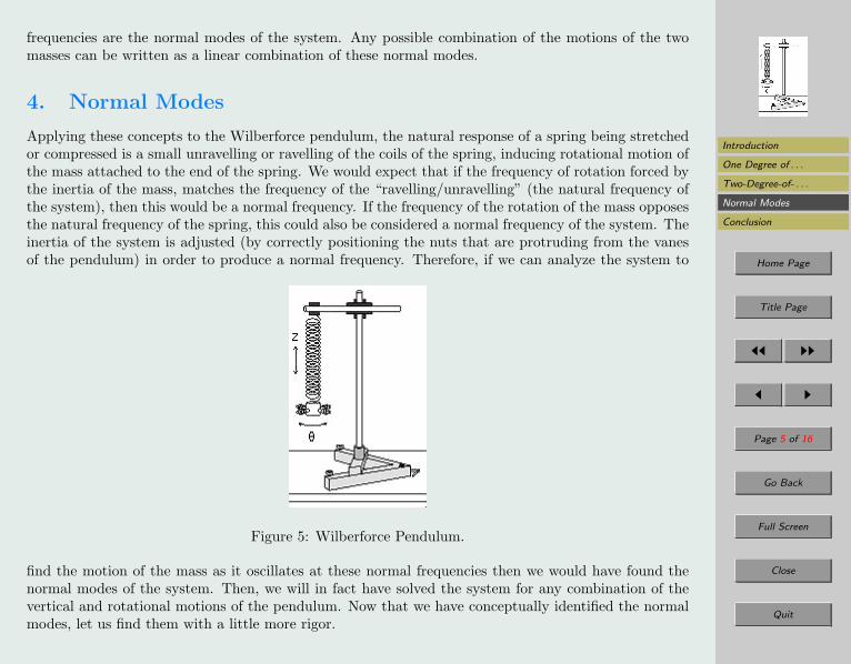
Applying these concepts to the Wilberforce pendulum, the natural response of a spring being stretchedor compressed is a small unravelling or ravelling of the coils of the spring, inducing rotational motion ofthe mass attached to the end of the spring. We would expect that if the frequency of rotation forced bythe inertia of the mass, matches the frequency of the “ravelling/unravelling” (the natural frequency ofthe system), then this would be a normal frequency. If the frequency of the rotation of the mass opposesthe natural frequency of the spring, this could also be considered a normal frequency of the system. Theinertia of the system is adjusted (by correctly positioning the nuts that are protruding from the vanesof the pendulum) in order to produce a normal frequency. Therefore, if we can analyze the system to

Figure 5: Wilberforce Pendulum.

find the motion of the mass as it oscillates at these normal frequencies then we would have found thenormal modes of the system. Then, we will in fact have solved the system for any combination of thevertical and rotational motions of the pendulum. Now that we have conceptually identified the normalmodes, let us find them with a little more rigor.

Introduction

One Degree of . . .


Normal Modes

Conclusion

Home Page

Title Page

JJ II

J I

of 16

Go Back

Full Screen

Close

Quit

In our system the vertical displacement is going to be measured from equilibrium in the z direction,and the displacement in rotation is going to be measured as an angle θ from equilibrium (see Figure 5).The Lagrangian for our system is the kinetic energy minus the potential energy plus a coupling termwith coupling constant ε. This coupling term accounts for the fact that the energy in the z direction isdependent on the energy in the θ direction, and visa-versa, where ε is the magnitude of this effect. ε isdependent on the properties of the spring. The kinetic energy (K) of the mass in the vertical directionis defined to be

12mv2 =

12z2,

and the potential energy (U) is given by12kz2.

Likewise the kinetic and potential energies of the mass in rotation are

12Iθ2 and

12δθ2

respectively, where I is the inertia of the mass and δ is the rotational spring constant. The couplingterm is a potential energy relation of z and θ, given by

12εzθ.

Therefore the Lagrangian (L) for this system is

L = K − U =12mz2 +

12Iθ2 − 1

2kz2 − 1

2δθ2 − 1

2εzθ. (1)

We need to minimize the Lagrangian for our system. The well-known Euler-Lagrange equations will dothis for us, in the same way that, to find the minimum of a function, we take its derivative and set itequal to zero.

d

dt

(∂L

∂z

)− ∂L

∂z= 0,

d

dt

(∂L

∂θ

)− ∂L

∂θ= 0, (2)

where the derivative with respect to time of the partial derivative of the Lagrangian with respect to zminus the partial derivative with respect to z equals zero. Also, the derivative with respect to time ofthe partial derivative with respect to θ minus the partial derivative with respect to θ equals zero.

Applying the Euler-Lagrangian equation to Equation (1) returns

Introduction

One Degree of . . .


Normal Modes

Conclusion

Home Page

Title Page

JJ II

J I

of 16

Go Back

Full Screen

Close

Quit

∂L

∂z= mz

∂L

∂z= −kz − 1

2εθ,

thus,

0 =d

dt

(∂L

∂z

)− ∂L

∂z

0 =d

dt(mz)−

(−kz − 1

2εθ

)0 = mz + kz +

12εθ.

In the same manner,

∂L

∂θ= Iθ

∂L

∂θ= −δθ − 1

2εz,

thus,

0 =d

dt

(∂L

∂θ

)− ∂L

∂θ

0 =d

dt

(Iθ

)−

(−δθ − 1

2εz

)0 = Iθ + δθ +

12εz.

These two second-order, non-homogeneous differential equations describe the complete motion of thesystem.

mz + kz +12εθ = 0 (3)

Iθ + δθ +12εz = 0 (4)

The first of these two equations describes the vertical motion of the mass. The second describes itsrotational motion. The terms 1

2εθ and 12εz couple the two motions, thereby making each a function of

both variables.

Introduction

One Degree of . . .


Normal Modes

Conclusion

Home Page

Title Page

JJ II

J I

of 16

Go Back

Full Screen

Close

Quit

Assuming the system to be in a normal mode, the masses can oscillate with the same frequency andphase angle but with different amplitudes. From well known oscillator theory, the solutions to Equations(3) and (4) can be assumed to be

z(t) = A1 cos (ωt + φ). (5)θ(t) = A2 cos (ωt + φ) (6)

We need to take the first and second derivatives of these equations with respect to t so that we can thensubstitute the result into Equations (3) and (4) to solve for the amplitudes of oscillation.

z(t) = −A1ω sin (ωt + φ)

θ(t) = −A2ω sin (ωt + φ)

z(t) = −A1ω2 cos (ωt + φ)

θ(t) = −A2ω2 cos (ωt + φ)

Substituting these equations back into Equations (3) and (4), we get

m(−A1ω2 cos (ωt + φ)) + kA1 cos (ωt + φ) +

12εA2 cos (ωt + φ) = 0

I(−A2ω2 cos (ωt + φ)) + δA2 cos (ωt + φ) +

12εA1 cos (ωt + φ) = 0.

Factoring out cos (ωt + φ) and dividing through by m, we get(k

m− ω2

)A1 +

ε

2mA2 = 0 (7)

ε

2IA1 +

(δ

I− ω2

)A2 = 0. (8)

We may set k/m and δ/I equal to ω2z and ω2

θ respectively, because these are the squares of the naturalfrequencies of the vertical and rotational motions. Then grouping A1 and A2 terms yields a system forwhich we can solve A1 and A2,

(ω2z − ω2)A1 +

ε

2mA2 = 0 (9)

ε

2IA1 + (ω2

θ − ω2)A2 = 0. (10)

Introduction

One Degree of . . .


Normal Modes

Conclusion

Home Page

Title Page

JJ II

J I

of 16

Go Back

Full Screen

Close

Quit

The trivial solution to this system

A =[A1

A2

]=

[00

]produces a motionless system because the magnitude of the amplitudes are zero, so we need non-trivialsolutions. To find non-trivial solutions of A1 and A2, the determinant of the coefficients of this systemof linear equations must be equal to zero.∣∣∣∣∣ω2

z − ω2 ε2m

ε2I ω2

θ − ω2

∣∣∣∣∣ = 0.

Expanding the determinant and grouping like terms yields

ω4 − (ω2z − ω2

θ)ω2 +(

ω2zω2

θ −ε2

4mI

)= 0.

Solving this equation for ω using a binomial expansion, we get the frequencies of the two normal modes.

ω21 =

12

{ω2

θ + ω2z +

√(ω2

θ − ω2z)2 +

ε2

mI

}

ω22 =

12

{ω2

θ + ω2z −

√(ω2

θ − ω2z)2 +

ε2

mI

}

Only when the frequency of oscillation of the mass is equal to the natural frequencies in z and θ can weobserve the system to oscillate in a normal mode. Recall the two-mass system. The masses were onlyable to oscillate with the same frequency because the spring constants of the two outside springs wereequal. Thus, when the natural frequency of the system in z equals the natural frequency of the systemin θ, then we can make the substitution ωθ = ωz = ω, and the above equations can be reduced to

ω21 = ω2 +

ε√mI

(11)

ω22 = ω2 − ε√

mI(12)

Introduction

One Degree of . . .


Normal Modes

Conclusion

Home Page

Title Page

JJ II

J I

of 16

Go Back

Full Screen

Close

Quit

If we let ωB = ε/2√

mI. These equations become

ω21 = ω2 +

ωB

2(13)

ω22 = ω2 − ωB

2(14)

ThusωB = ω1 − ω2,

where ωB is the beat frequency produced by the interference of the two normal frequencies.Now that we have the normal frequencies, we need to know the relation of the amplitudes of oscillation

in z and θ. The ratio of those amplitudes is dependent on the frequency of the normal mode. Since wechose an ω that makes Equations (9) and (10) dependent, we only need to solve Equation (9) for theratio of the amplitudes at the first normal frequency by substituting ω2

1 for ω2. Equation (9) becomes

(ω2z − ω2

1)A1 +ε

2mA2 = 0,

but ω21 = ω2 + ε/

√4mI from Equation (10) and ω2

z = ω2. So the above equation becomes

− ε√4mI

A1 +ε

2mA2 = 0.

Solving for A2/A1 yields√

m/I. Doing the same for the second normal frequency, we get the ratio atω2. It turns out that

A2

A1= r1 =

√m

I= −r2,

where r1 and r2 are the ratios of the amplitudes at each normal frequency. Therefore, the amplitudevectors can be written as

A(1) =

A(1)1

A(1)2

=

A(1)1

r1A(1)1

A(2) =

A(2)1

A(2)2

=

A(2)1

r2A(2)1

,

Introduction

One Degree of . . .


Normal Modes

Conclusion

Home Page

Title Page

JJ II

J I

of 16

Go Back

Full Screen

Close

Quit

where superscript denotes the frequency at which the Amplitude was obtained. The solutions for themotions of system thus can be written as position vectors,

x(1) =

z(1)(t)

θ(1)(t)

=

A(1)1 cos (ω1t + φ1)

r1A(1)1 cos (ω1t + φ1)

= first mode

x(2) =

z(2)(t)

θ(2)(t)

=

A(2)1 cos (ω2t + φ2)

r2A(2)1 cos (ω2t + φ2)

= second mode

Again we remind you that any motion of the pendulum can be written as a linear combination of itsnormal modes. Thus,

z(t) = z(1)(t) + z(2)(t) = A(1)1 cos (ω1t + φ1) + A

(2)1 cos (ω2t + φ2) (15)

θ(t) = θ(1)(t) + θ(2)(t) = A(1)2 r1 cos (ω1t + φ1) + A

(2)2 r2 cos (ω2t + φ2) (16)

The initial conditions that we give our pendulum are a twist and a displacement in the z direction,but no initial velocity in either direction. Therefore, the initial conditions are

z(0) = z0 z(0) = 0

θ(0) = θ0 θ(0) = 0.

Substituting these initial conditions into Equations (15) and (16), the equations that we will use todetermine the amplitudes A

(1)1 and A

(2)1 and the phase angles φ1 and φ2 are

z0 = A(1)1 cos φ1 + A

(2)1 cos φ2

0 = −ω1A(1)1 sinφ1 − ω2A

(2)1 sinφ2

θ0 = r1A(1)1 cos φ1 + r2A

(2)1 cos φ2

0 = −r1ω1A(1)1 sinφ1 − r2ω2A

(2)1 sinφ2.

Solving this system for A(1)1 , A

(2)1 , φ1, and φ2

A(1)1 =

r1θ0 + z0

r1 − r2, A

(2)1 =

r1θ0 − z0

r1 − r2, φ1 = φ2 = 0.

Introduction

One Degree of . . .


Normal Modes

Conclusion

Home Page

Title Page

JJ II

J I

of 16

Go Back

Full Screen

Close

Quit

Substituting√

m/I for r1, and −√

m/I for r2, the general solution of the motion of the Wilberforcependulum is

z(t) =

√mI θ0 + z0

2√

mI

cos ω1t +

√mI θ0 − z0

2√

mI

cos ω2t

θ(t) =√

m

I

√mI θ0 + z0

2√

mI

cos ω1t−√

m

I

√mI θ0 − z0

2√

mI

cos ω2t.

5. Conclusion

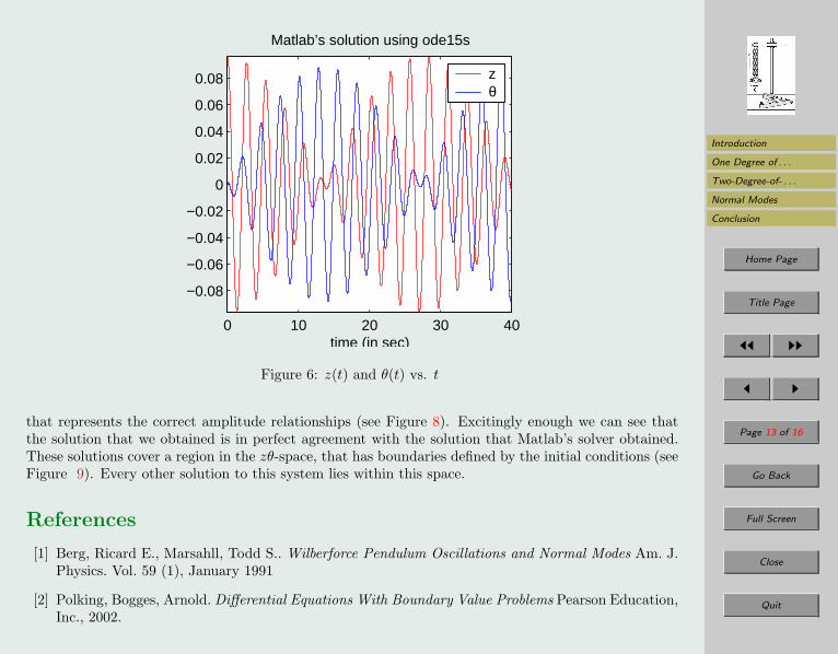
Let us look at the solution of the system of differential equations, Equations (3) and (4), plotted usingMatlab’s built-in ode15s m-file, so as to have something to compare our solutions to (see Figure 6). Ourconstants are set to those measured by Berg and Marshal [1, p.35], and tabulated in the table below.

Inertia (I) 1.45E−4 Nm2

Mass (m) 0.5164 kg

Epsilon (ε) 9.28E−3 N

Torsional spring constant (δ) 7.86E−4 Nm2

Longitudinal spring constant (k) 2.69 N/m

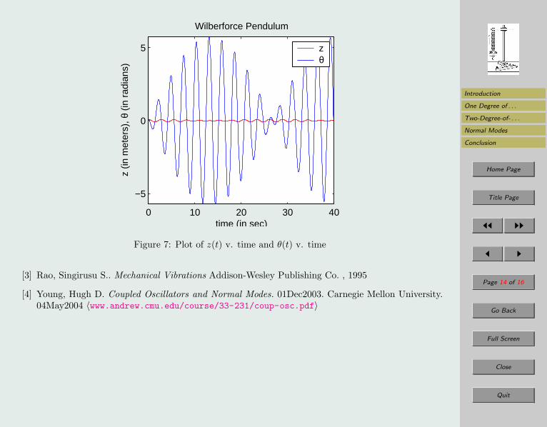
Now let us plot our solutions using the same constants. See Figure 7 for a plot of our solutions versustime.

The first thing we notice is beating occurring, showing the complete transfer of kinetic energy fromz to θ and back. The next thing we notice is that the displacement of the mass in the vertical directionis disproportional to the displacement of the mass’ rotation. So the ratio of the amplitudes appearnot to match our previous computations, but intuitively this is to be expected because of the smalldisplacement in rotation that the mass experiences in relation to its large vertical displacement. Toremedy this discrepancy, we need to put the displacement of rotation into units of the z displacement.If we change the θ displacement into arc length (s) by the relationship s = rθ, we can obtain a plot

Introduction

One Degree of . . .


Normal Modes

Conclusion

Home Page

Title Page

JJ II

J I

of 16

Go Back

Full Screen

Close

Quit

0 10 20 30 40

−0.08

−0.06

−0.04

−0.02

0

0.02

0.04

0.06

0.08

time (in sec)

met

ers

Matlab’s solution using ode15s

zθ

Figure 6: z(t) and θ(t) vs. t

that represents the correct amplitude relationships (see Figure 8). Excitingly enough we can see thatthe solution that we obtained is in perfect agreement with the solution that Matlab’s solver obtained.These solutions cover a region in the zθ-space, that has boundaries defined by the initial conditions (seeFigure 9). Every other solution to this system lies within this space.

References

[1] Berg, Ricard E., Marsahll, Todd S.. Wilberforce Pendulum Oscillations and Normal Modes Am. J.Physics. Vol. 59 (1), January 1991

[2] Polking, Bogges, Arnold. Differential Equations With Boundary Value Problems Pearson Education,Inc., 2002.

Introduction

One Degree of . . .


Normal Modes

Conclusion

Home Page

Title Page

JJ II

J I

of 16

Go Back

Full Screen

Close

Quit

0 10 20 30 40

−5

0

5

time (in sec)

z (in

met

ers)

, θ (

in r

adia

ns)

Wilberforce Pendulum

zθ

Figure 7: Plot of z(t) v. time and θ(t) v. time

[3] Rao, Singirusu S.. Mechanical Vibrations Addison-Wesley Publishing Co. , 1995

[4] Young, Hugh D. Coupled Oscillators and Normal Modes. 01Dec2003. Carnegie Mellon University.04May2004 〈www.andrew.cmu.edu/course/33-231/coup-osc.pdf〉

www.andrew.cmu.edu/course/33-231/coup-osc.pdf

Introduction

One Degree of . . .


Normal Modes

Conclusion

Home Page

Title Page

JJ II

J I

of 16

Go Back

Full Screen

Close

Quit

0 10 20 30 40

−0.08

−0.06

−0.04

−0.02

0

0.02

0.04

0.06

0.08

time (in sec)

met

ers

Wilberforce Pendulum

zθ

Figure 8: Plot of z(t) v. time and θ(t) v. time

Introduction

One Degree of . . .


Normal Modes

Conclusion

Home Page

Title Page

JJ II

J I

of 16

Go Back

Full Screen

Close

Quit

−0.1 −0.05 0 0.05 0.1

−0.08

−0.06

−0.04

−0.02

0

0.02

0.04

0.06

0.08

z (in meters)

θ (in

met

ers)

Normal modes in the z−θ space

Figure 9: The Space Containing the Normal Modes

basic coupled oscillator theory applied to the wilberforce ... · pdf filebasic coupled...

Documents