BASIC ECONOMIC CONCEPTSCourse Notes

Costas Courcoubetis

Abstract

These notes are about basic concepts in economics that are needed in order to studyissues of pricing information goods and telecommunication services. They consist of materialextracted from Chapters 5 and 6 of the book Pricing Communication Networks: Economics,Technology and Modeling, Wiley 2003, by C. Courcoubetis and R. Weber. There are twoparts. In the first part we study some basic conceps including user utility, demand andsocial welfare. In the second part we study certain basic competition models modelling theactual market conditions. The text in blue may be skipped on a first reading.

1

Contents

PART A: Basic Concepts 4

1 Charging for services 4

1.1 Demand, supply and market mechanisms . . . . . . . . . . . . . . . . . . . . . . 4

1.2 Charge, tariff and price . . . . . . . . . . . . . . . . . . . . . . . . . . . . . . . . 4

1.3 Contexts for deriving prices . . . . . . . . . . . . . . . . . . . . . . . . . . . . . . 4

2 The consumer’s problem 6

2.1 Utility function, surplus maximization and demand function . . . . . . . . . . . . 6

2.2 Elasticity . . . . . . . . . . . . . . . . . . . . . . . . . . . . . . . . . . . . . . . . 8

2.3 Cross-elasticities, substitutes and complements . . . . . . . . . . . . . . . . . . . 9

3 The supplier’s problem 9

4 Welfare maximization 10

4.1 The case of producer and consumers . . . . . . . . . . . . . . . . . . . . . . . . . 11

4.1.1 Iterative price adjustment: network and user interaction . . . . . . . . . . 13

4.2 The case of consumers and finite capacity constraints . . . . . . . . . . . . . . . . 14

4.3 Discussion of marginal cost pricing . . . . . . . . . . . . . . . . . . . . . . . . . . 14

4.4 Recovering costs . . . . . . . . . . . . . . . . . . . . . . . . . . . . . . . . . . . . 15

4.5 Walrasian equilibrium . . . . . . . . . . . . . . . . . . . . . . . . . . . . . . . . . 17

4.6 Pareto efficiency . . . . . . . . . . . . . . . . . . . . . . . . . . . . . . . . . . . . 18

5 Network externalities 20

PART B: Competition Models 22

6 Types of competition 22

7 Monopoly 24

7.1 Profit maximization . . . . . . . . . . . . . . . . . . . . . . . . . . . . . . . . . . 24

7.2 Price discrimination . . . . . . . . . . . . . . . . . . . . . . . . . . . . . . . . . . 25

7.3 Bundling . . . . . . . . . . . . . . . . . . . . . . . . . . . . . . . . . . . . . . . . 30

7.4 Service differentiation and market segmentation . . . . . . . . . . . . . . . . . . . 31

8 Perfect competition 32

8.1 Competitive markets . . . . . . . . . . . . . . . . . . . . . . . . . . . . . . . . . . 33

8.2 Lock-in . . . . . . . . . . . . . . . . . . . . . . . . . . . . . . . . . . . . . . . . . 34

2

9 Oligopoly 36

9.1 Games . . . . . . . . . . . . . . . . . . . . . . . . . . . . . . . . . . . . . . . . . . 36

3

1 Charging for services

1.1 Demand, supply and market mechanisms

Communication services are valuable economic commodities. The prices for which they can be

sold depend on factors of demand, supply and how the market operates. The key players in the

market for communications services are suppliers, consumers, and regulators. The demand for

a service is determined by the value users place upon it and the price they are willing to pay

to obtain it. The quantity of the service that is supplied in the market depends on how much

suppliers can expect to charge for it and on their costs. Their costs depend on the efficiency

of their network operations. The nature of competition amongst suppliers, how they interact

with customers, and how the market is regulated all have a bearing on the pricing of network

services.

One of the most important factors is competition. Competition is important because it tends

to increases economic efficiency: that is, it increases the aggregate value of the services that

are produced and consumed in the economy. Sometimes competition does not occur naturally.

In that case, regulation by a government agency can increase economic efficiency. By imposing

regulations on the types of tariffs, or on the frequency with which they may change, a regulator

can arrange for there to be a greater aggregate welfare than if a dominant supplier were allowed

to produce services and charge for them however he likes. Moreover, the regulator can take

account of welfare dimensions that suppliers and customers might be inclined to ignore. For

example, a regulator might require that some essential network services be available to everyone,

no matter what their ability to pay. Or he might require that encrypted communications can be

deciphered by law enforcement authorities. He could take a ‘long term view’, or adopt policies

designed to move the market in a certain desirable direction.

1.2 Charge, tariff and price

It is useful to give distinct meanings to the words ‘charge’, ‘tariff’ and ‘price’. We say that a

supplier charges customers for network services. The charge that a customer pays is computed

from a tariff . This tariff can be a complex function and take account of various aspects of the

service and perhaps measurements of the customer’s usage. For example, a telephone service

might tariffed in terms of monthly rental, the numbers of calls that are made, their durations,

the times of day at which they are made, and whether they are local or long-distance.

A price is a charge that is associated with one unit of usage. For example, a mobile phone

service provider might operate a two-part tariff of the form a + bx, where a is a monthly

fixed-charge (or access charge), x is the number of minutes of calling per month, and b is the

price per minute.

1.3 Contexts for deriving prices

In thinking about how price are determined there are two important questions to answer: (a)

who sets the price, and (b) with what objective? It is interesting to look at three different

4

answers and the rationales that they give for thinking about prices. The first answer is that

sometimes the market that sets the price, and the objective is to match supply and demand.

Supply and demand at given prices depend on the supplier’s technological capacities, the costs

of supply, and the how consumers value the service. If prices are set too low then there will be

insufficient incentive to supply and there is likely to be unsatisfied demand. If prices are set too

high then suppliers may oversupply the market and find there is insufficient demand at that

price. The ‘correct’ price should be ‘market-clearing’. That is, it should be the price at which

demand exactly equals supply.

A second rationale for setting prices comes about when it is the producer who sets prices

and his objective is to deter potential competitors. Imagine a game in which an incumbent firm

wishes to protect itself against competitors who might enter the market. This game takes place

under certain assumptions about both the incumbent’s and entrants’ production capabilities and

costs. We find that if the firm is to be secure against new entrants seducing away some of its

customers, then the charges that it makes for different services must satisfy certain constraints.

For example, if a firm uses the revenue from selling one product to subsidize the cost of producing

another, then the firm is in danger if a competitor can produce only the first product and sell

it for less. This would lead to a constraint of no cross-subsidization.

A third rationale for setting prices comes about when a principal uses prices as a mechanism

to induce an agent to take certain actions. The principal cannot dictate directly the actions

he wishes the agent to take, but he can use prices to reward or penalize the agent for actions

that are or are not desired. Let us consider two examples. In our first example the owner of a

communications network is the principal and the network users are the agents. The principal

prices the network services to motivate users to choose services that both match their needs

and avoid wasting network resources. Suppose that he manages a dial-in modem bank. If he

prices each unit of connection time, then he gives users the incentive to disconnect when they

are idle. His pricing is said to be incentive compatible. That is, it provides an incentive that

induces desirable user response. A charge based only on pricing each byte that is sent would

not be incentive compatible in this way.

In our second example the owner of the communications network is now the agent. A

regulator takes the role of principal and uses price regulation to induce the network owner to

improve his infrastructure, increase his efficiency, and provide the services that are of value to

consumers.

These are three possible rationales for setting prices. They do not necessarily lead to the

same prices. We must live with the fact that there is no single recipe for setting prices that

takes precedence over all others. Pricing can depend on the underlying context, or contexts,

and on contradictory factors. This means that the practical task of pricing is as much an art

as a science. It requires a good understanding of the particular circumstances and intricacies

of the market.

It is not straightforward even to define the cost of a good. For example, there are many

5

different approaches to defining the cost of a telephone handset. It could be the cost of the

handset when it was purchased (the historical cost), or its opportunity cost (the value of what

we must give up to produce it), or the cost of the replacing it with a handset that has the same

features (its modern equivalent asset cost). In these notes we assume that the notion of the

cost is unambiguously defined.

2 The consumer’s problem

2.1 Utility function, surplus maximization and demand function

Consider a market in which n customers can buy k services. Denote the set of customers by

N = {1, . . . , n}. Customer i can buy a vector quantity of services x = (x1, . . . , xk) for a payment

of p(x). Let us suppose that p(x) = p�x =∑

j pjxj , for a given vector of prices p = (p1, . . . , pk).

Assume that the available amounts of the k services are unlimited and that customer i seeks to

solve the problem

xi(p) = arg maxx

[ui(x) − p�x

]. (1)

Here ui(x) is the utility to customer i of having the vector quantities of services x. One can

think of ui(x) as the amount of money he is willing to pay to receive the bundle that consists

of these services in quantities x1 . . . , xk. Equivalently, it is the revenue the user can obtain by

reselling the

It is usual to assume that ui(·) is strictly increasing and strictly concave for all i. This

ensures that there is a unique maximizer in (1) and that demand decreases with price. If,

moreover, u(·) is differentiable, then the marginal utility of service j, as given by ∂ui(x)/∂xj , is

a decreasing function of xj . We make these assumptions unless we state otherwise. However, we

note that there are cases in which concavity does not hold. For example, certain video coding

technologies can operate only when the rate of the video stream is above a certain minimum,

say x∗, of a few megabits per second. A user who wishes to use such a video service will have

a utility that is zero for a rate x that is less than x∗ and positive for x at x∗. This is a step

function and not concave. The utility may increase as x increases above x∗, since the quality

of the displayed video increases with the rate of the encoding. This part of the utility function

may be concave, but the utility function as a whole is not. In practice, for coding schemes like

MPEG, the utility function is not precisely a step function, but it resembles one. It starts at

zero and increases slowly until a certain bit rate is attained. After this point it increases rapidly,

until it eventually reaches a maximum value. The first part of the curve captures the fact that

the coding scheme cannot work properly unless a certain bit rate is available.

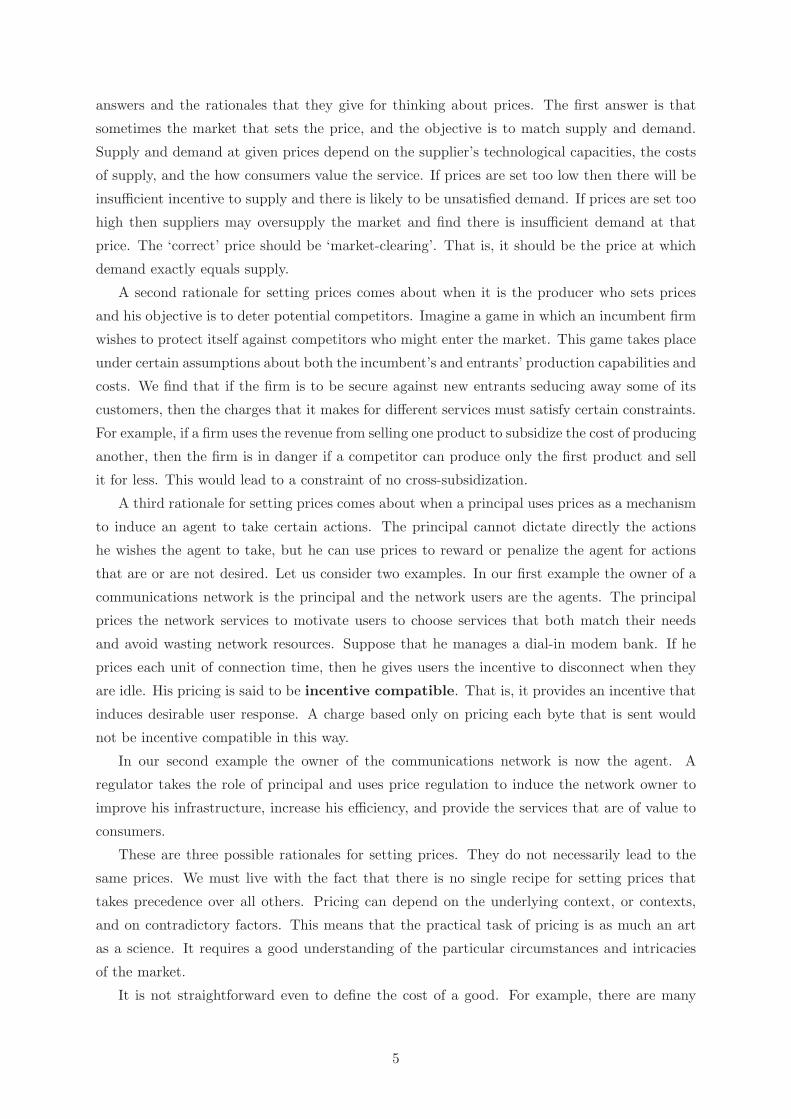
The expression that is maximized on the right hand side of (1) is called the consumer’s net

benefit or consumer surplus,

CSi = maxx

[ui(x) − p�x] .

It represents the net value the consumer obtains as the utility of x minus the amount paid for

x. The above relations are summarized in Figure 1.

6

utility u(x)

px

x0 x(p)

maximized net benefit

= max [u(x) − px]

Figure 1: The consumer has a utility u(x) for a quantity x of a service. In this figure, u(x) is increasingand concave. Given the price vector p, the consumer chooses to purchase the amount x = x(p) thatmaximizes his net benefit (or consumer surplus). Note that at x = x(p) we have ∂u(x)/∂x = p.

he vector xi(p) is called the demand function for customer i. It gives the quantities

xi = (xi1, . . . , x

ik) of services that customer i will buy if the price vector is p. The aggregate

demand function is x(p) =∑

i∈N xi(p); this adds up the total demand of all the users at

prices p. Similarly, the inverse aggregate demand function, p(x), is the vector of prices at

which the total demand is x.

Consider the case of a single customer who is choosing the quantity to purchase of just a

single service, say service j. Imagine that the quantities of all other services are held constant

and provided to the customer for no charge. If his utility function u(·) is concave and twice

differentiable in xj then his net benefit, of u(x)−pjxj , is maximized where it is stationary point

with respect to xj , i.e., where ∂u(x)/∂xj = pj . At this point the marginal increase in utility due

to increasing xj is equal to the price of j. We also see that the customer’s inverse demand

function is simply pj(xj) = ∂u(x)/∂xj . It is the price at which he will purchase a quantity

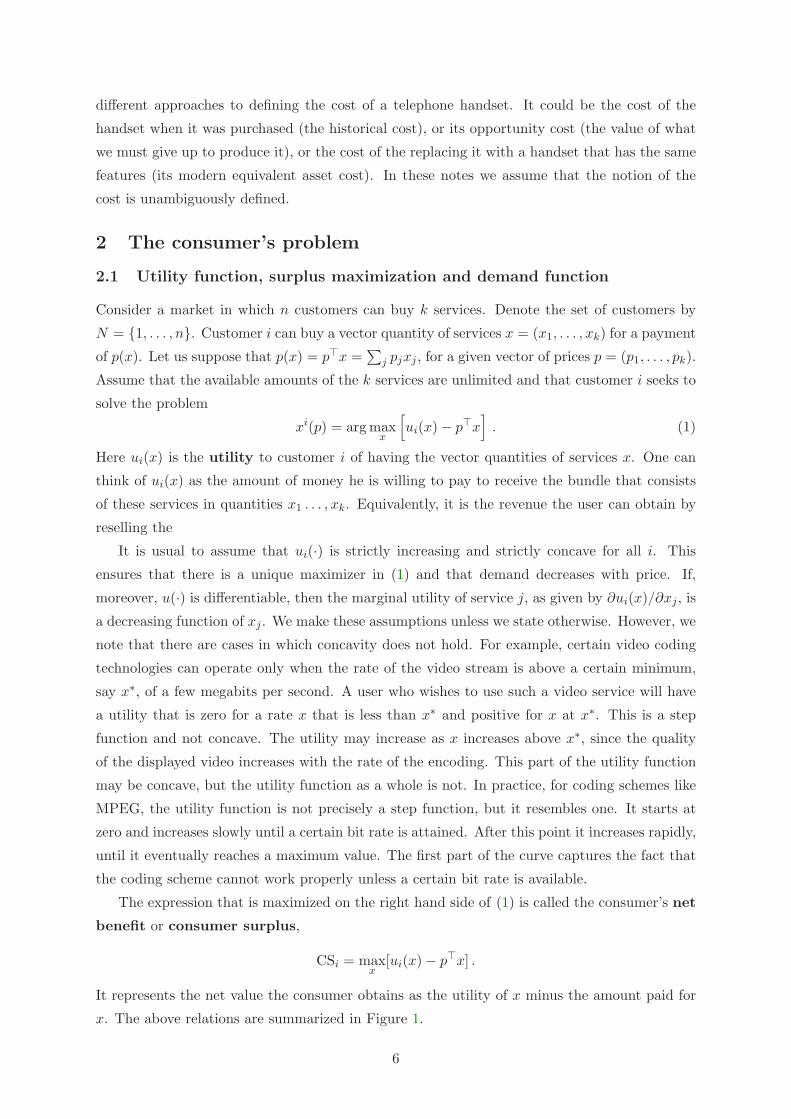
xj . Thus, for a single customer who purchases a single service j, we can express his consumer

surplus at price pj as

CS(pj) =∫ xj(pj)

0pj(x) dx − pjxj(pj) . (2)

We illustrate this in Figure 2 (dropping the subscript j).

We make a final observation about (1). We have implicitly assumed that the (per unit)

prices charged in the market are the same for all units purchased by the customer. There are

more general pricing mechanisms in which the charge paid by the customer for purchasing a

quantity x is a more general function r(x), not of the form p�x. For instance, prices may depend

on the total amount bought by a customer, as part of nonlinear tariffs, of the sort we examine

in Section 7.2. Unless explicitly stated, we use the term ‘price’ to refer to the price that defines

a linear tariff p�x.

The reader may also wonder how general is (1) in expressing the net benefit of the customer

as a difference between utility and payment. Indeed, a more general version is as follows. A

7

0 x

p

px

x(p)

u′(x)

CS(p)

$

Figure 2: The demand curve for the case of a single customer and a single good. The derivative ofu(x), denoted u′(x), is downward sloping, here for simplicity shown as a straight line. The area underu′(x) between 0 and x(p) is u(x(p)), and so subtracting px (the area of the shaded rectangle) gives theconsumer surplus as the area of the shaded triangle.

customer has a utility function v(x0, x) where x0 is his net income (say in dollars), and x is the

vector of goods he consumes. Then at price p he solves the problem

xi(p) = arg{

maxx

v(x0 − p�x, x) : p�x ≤ x0

}.

In the simple case that the customer has a quasilinear utility function, of the form v(x0, x) =

x0 +u(x), and assuming his income is large enough that x0 − p�x > 0 at the optimum, he must

solve a problem that is equivalent to (1). It is valid to assume a quasilinear utility function

when the customer’s demand for services is not very sensitive to his income, i.e., expenditure

is a small proportion of his total income, and this is the case for most known communications

services. In our economic modelling we use these assumptions regarding utility functions since

they are reasonable and simplify significantly the mathematical formulas without reducing the

qualitative applicability of the results.

2.2 Elasticity

Concavity of u(·) ensures that both x(p) and p(x) are decreasing in their arguments, or as

economists say, downward sloping. As price increases, demand decreases. A measure of this

is given by the price elasticity of demand. Customer i has elasticity of demand for service

j given by

εj =∂xj(p)/∂pj

xj/pj,

where for simplicity we omit the superscript i in the demand vector xi since we refer to a single

customer. Thus∆xj

xj= εj

∆pj

pj,

8

and elasticity measures the percentage change in the demand for a good per percentage change

in its price. Recall that the inverse demand function satisfies pj(x) = ∂u(x)/∂xj . So the

concavity of the utility function implies ∂pj(x)/∂xj ≤ 0 and εj is negative.1 As |εj | is greater or

less than 1 we say that demand of customer i for service j is respectively elastic or inelastic.

Note that since we are working in percentages, εj does not depend on the units in which xj or pj

is measured. However, it does depend on the price, so we must speak of the ‘elasticity at price

pj ’. The only demand function for which elasticity is the same at all prices is one of the form

x(p) = apε. One can define other measures of elasticity, such ‘income elasticity of demand’,

which measures the responsiveness of demand to a change in a consumer’s income.

2.3 Cross-elasticities, substitutes and complements

Sometimes the demand for one good can depend on the prices of other goods. We define the

cross elasticity of demand, εjk, as the percentage change in the demand for good j per

percentage change in the price of another good, k. Thus

εjk =∂xj(p)/∂pk

xj/pk

and∆xj

xj= εjk

∆pk

pk.

But why should the price of good k influence the demand for good j? The answer is that

goods can be either substitutes or complements. Take, for example, two services of different

quality such as VBR and ABR in ATM. If the price for VBR increases, then some customers

who were using VBR services, and who do not greatly value the higher quality of VBR over

ABR, will switch to ABR services. Thus the demand for ABR will increase. The services are

said to be substitutes. The case of complements is exemplified by network video transport

services and video conferencing software. If the price of one of these decreases, then demand

for both increases, since both are needed to provide the complete video conferencing service.

Formally, services j and k are substitutes if ∂xj(p)/∂pk > 0 and complements if ∂xj(p)/∂pk <

0. If ∂xj(p)/∂pk = 0, the services are said to be independent. Surprisingly, the order of the

indices j and k is not significant. To see this, recall that the inverse demand function satisfies

pj(x) = ∂u(x)/∂xj . Hence ∂pj(x)/∂xk = ∂pk(x)/∂xj , and so the demand functions satisfy

∂xj(p)∂pk

=∂xk(p)

∂pj.

3 The supplier’s problem

Suppose that a supplier produces quantities of k different services. Denote by y = (y1, . . . , yk)

the vector of quantities of these services. For a given network and operating method the1Authors disagree in the definition of elasticity. Some define it as the negative of what we have, so that it

comes out positive. This is no problem provided one is consistent.

9

supplier is restricted to choosing y within some set, say Y , usually called the technology set

or production possibilities set in the economics literature.

Profit, or producer surplus, is the difference between the revenue that is obtained from

selling these services, say r(y), and the cost of production, say c(y). An independent firm having

the objective of profit maximization, seeks to solve the problem of maximizing the profit,

π = maxy∈Y

[r(y) − c(y)] .

An important simplification of the problem takes place in the case of linear prices, when

r(y) = p�y for some price vector p. Then the profit is simply a function of p, say π(p), as is

also the optimizing y, say y(p). Here y(p) is called the supply function, since it gives the

quantities of the various services that the supplier will produce if the prices at which they can

be sold is p.

The way in which prices are determined depends on the prevailing market mechanism. We

can distinguish three important cases. If the supplier is a monopolist, that is, the sole supplier

in an unregulated monopoly, then he is free to set whatever prices he wants. His choice is

constrained only by the fact that as he increases the prices of services the customers are likely

to buy less of them.

If the supplier is a small player amongst many, or prices are determined by a regulator, then

he may have no control over p, and thus he is a price-taker, with no freedom except his choice

of y. This is a typical case. An appropriate model is linear prices which independent of the

quantity sold. This is also the case for a regulated monopoly, where the price vector p is

fixed by the regulator, and the supplier simply supplies the services that the market demands

at the given price p.

A middle case, in which a supplier has partial influence over p, is when he is in competition

with a few others. In such an economy, or so-called oligopoly, suppliers compete for customers

through their choices of p and y. This assumes that suppliers do not collude or form a cartel.

They compete against one another and the market prices of services emerge as the solution to

some non-cooperative game.

4 Welfare maximization

Social welfare (which is also called social surplus) is defined as the sum of all users’ net

benefits, i.e., the sum of all consumer and producer surpluses. Note that weighted sums of

consumer and producer surpluses can be considered, reflecting the reality that a social plan-

ner/regulator/politician may attach more weight to one sector of the economy than to another.

We speak interchangeably of the goals of social welfare maximization, social surplus maximiza-

tion, and ‘economic efficiency’. The key idea is that, under certain assumptions about the

concavity and convexity of utility and cost functions, the social welfare can be maximized by

setting an appropriate price and then allowing producers and consumers to choose their opti-

mal levels of production and consumption. This has the great advantage of maximizing social

10

welfare in a decentralized way.

We will begin by supposing that the social welfare maximizing prices are set by a supervising

authority, such as a regulator of the market. Suppliers and consumers see these prices and then

optimally choose their levels of production and demand. They do this on the basis of information

they know. A supplier sets his level of production knowing only his own cost function, not the

consumers’ utility functions. A consumer sets his level of demand knowing only his own utility

function, not the producers’ cost functions or other customers’ utility functions. Individual

consumer’s utility functions are private information, but aggregate demand is commonly known.

Later we will discuss perfectly competitive markets, i.e., a markets in which no individual

consumer or producer is powerful enough to control prices, and so all participants must be price

takers. It is often the case that once prices settle to values at which demand matches supply,

the social welfare is maximized. Thus a perfectly competitive market can sometimes need no

regulatory intervention. This is not true, however, if there is some form of market failure, such

as that caused by externalities. In Section 5 we see, for example, how a market with strong

network externality effects may remain small and never actually reach the socially desirable

point of large penetration.

4.1 The case of producer and consumers

We begin by modelling the problem of the social planner who by regulation can dictate the

levels of production and demand so as to maximize social welfare. Suppose there is one producer,

and a set of consumers, N = {1, . . . , n}. Let xi denote the vector of quantities of k services

consumed by consumer i. Let x = x1 + · · · + xn denote the total demand and let c(x) denote

the producer’s cost to produce x. The social welfare (or surplus), S, is the total utility of the

services consumed minus their cost of production, and so is written

S =∑i∈N

ui(xi) − c(x) .

Since the social planner takes an overall view of network welfare let us label his problem as

SYSTEM : maximizex,x1,...,xn

∑i∈N

ui(xi) − c(x) , subject to x = x1 + · · · + xn.

Assume that each ui(·) is concave and c(·) is convex.2 Then SYSTEM can be solved by use of a

Lagrange multiplier p on the constraint x = x1 + · · ·+ xn. That is, for the right value of p, the

solution can be found by maximizing the Lagrangian

L =∑i∈N

ui(xi) − c(x) + p�(x − x1 − · · · − xn)

freely over x1, . . . , xn and x. Now we can write

L = CS + π , (3)2This is typically the case when the production facility cannot be expanded in the time frame of reference,

and marginal cost of production increases due to congestion effects in the facility. In practice, the cost functionmay initially be concave, due to economies of scale, and eventually become convex due to congestion. In thiscase, we imagine that the cost function is convex for the output levels of interest.

11

where

CS =∑i∈N

[ui(xi) − p�xi

]and π = p�x − c(x) .

In (3) we have written L as the sum of two terms, each of which is maximized over different

variables. Hence, for the appropriate value of the Lagrange multiplier p (also called a dual

variable), L is maximized by maximizing each of the terms individually. The first term is the

aggregate consumers’ surplus, CS. Following the previous observation, the consumers are

individually posed the set of problems

CONSUMERi : maximizexi

[ui(xi) − p�xi

], i = 1, . . . , n . (4)

The second term is the producer’s profit, π. The producer is posed the problem

PRODUCER : maximizex

[p�x − c(x)

]. (5)

Thus we have the remarkable result that the social planner can maximize social surplus by

setting an appropriate price vector p. In practice it can be easier for him to control the dual

variable p, rather than to control the primal variables x, x1, . . . , xn directly.

This price controls both production and consumption. Against this price vector, the con-

sumers maximize their surpluses and the producer maximizes his profit. Moreover, from (4)–(5)

we see that provided the optimum occurs for 0 < xij < ∞, this price vector satisfies

∂ui(xi)∂xi

j

=∂c(x)∂xj

= pj .

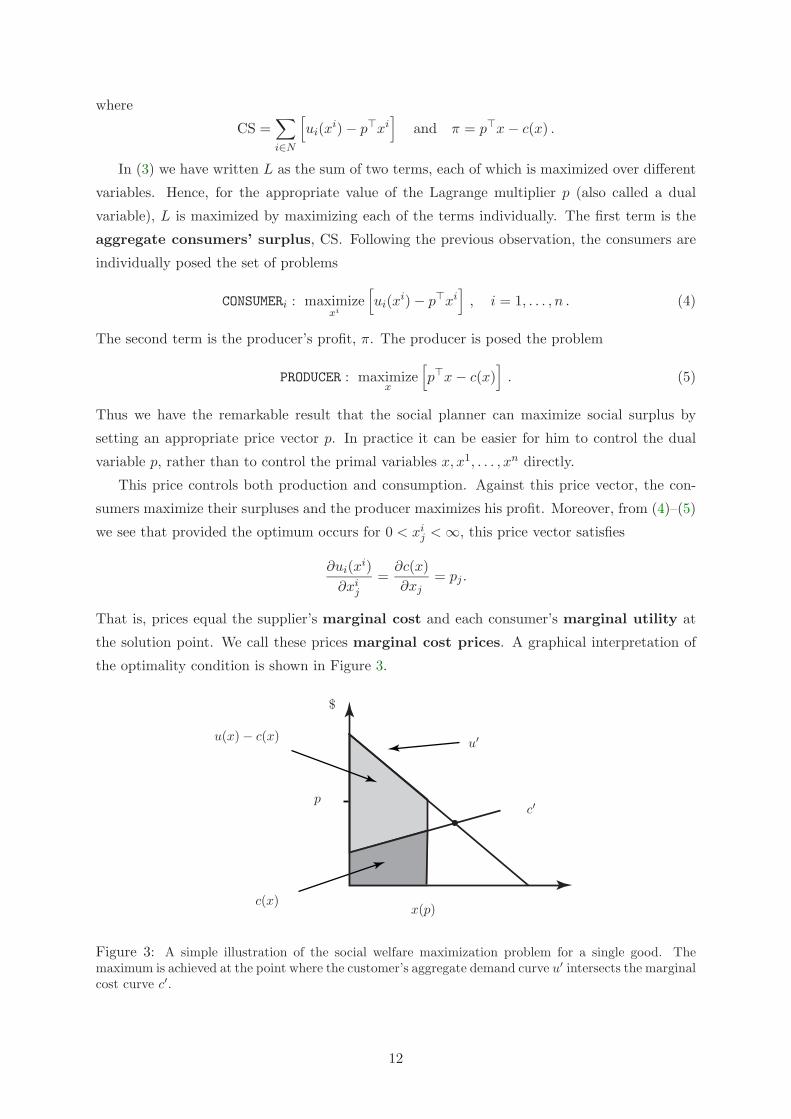
That is, prices equal the supplier’s marginal cost and each consumer’s marginal utility at

the solution point. We call these prices marginal cost prices. A graphical interpretation of

the optimality condition is shown in Figure 3.

u(x) − c(x)

c(x)

u′

c′p

x(p)

$

Figure 3: A simple illustration of the social welfare maximization problem for a single good. Themaximum is achieved at the point where the customer’s aggregate demand curve u′ intersects the marginalcost curve c′.

12

We have called the problem of maximizing social surplus the SYSTEM problem and have

seen that price is the catalyst for solving it, through decentralized solution of PRODUCER and

CONSUMERi problems. The social planner, or regulator, sets the price vector p. Once he has

posted p the producer and each consumer maximizes his own net benefit (of supplier profit or

consumer surplus). The producer automatically supplies x if he believes he can sell this quantity

at price p. He maximizes his profit by taking x such that for all j, either pj = ∂c(x)/∂xj ,

or xj = 0 if pj = 0. The social planner need only regulate the price; the price provides

a control mechanism that simultaneously optimizes both the demand and level of production.

We have assumed in the above that the planner attaches equal weight to consumer and producer

surpluses. In this case, the amount paid by the consumers to the producer is a purely internal

matter in the economy, which has no effect upon the resulting social surplus.

The same result holds if there is a set M of producers, the output of which is controlled

by the social planner to meet an aggregate demand at minimum total cost. Using the same

arguments as in the case of a single producer, the maximum of

S =∑i∈N

ui(xi) −∑j∈M

cj(yj) ,

subject to∑

i∈N xi =∑

j∈M yj , is achieved by

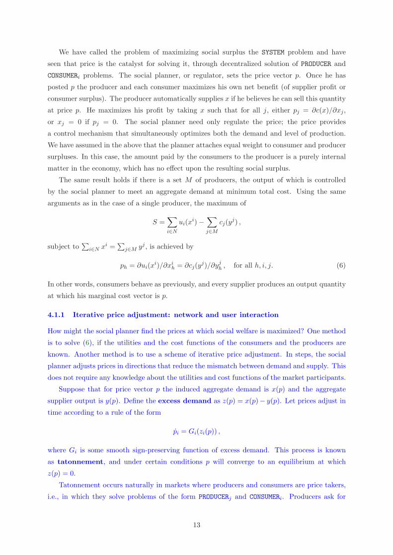
ph = ∂ui(xi)/∂xih = ∂cj(yj)/∂yj

h , for all h, i, j. (6)

In other words, consumers behave as previously, and every supplier produces an output quantity

at which his marginal cost vector is p.

4.1.1 Iterative price adjustment: network and user interaction

How might the social planner find the prices at which social welfare is maximized? One method

is to solve (6), if the utilities and the cost functions of the consumers and the producers are

known. Another method is to use a scheme of iterative price adjustment. In steps, the social

planner adjusts prices in directions that reduce the mismatch between demand and supply. This

does not require any knowledge about the utilities and cost functions of the market participants.

Suppose that for price vector p the induced aggregate demand is x(p) and the aggregate

supplier output is y(p). Define the excess demand as z(p) = x(p)− y(p). Let prices adjust in

time according to a rule of the form

pi = Gi(zi(p)) ,

where Gi is some smooth sign-preserving function of excess demand. This process is known

as tatonnement, and under certain conditions p will converge to an equilibrium at which

z(p) = 0.

Tatonnement occurs naturally in markets where producers and consumers are price takers,

i.e., in which they solve problems of the form PRODUCERj and CONSUMERi. Producers ask for

13

lower prices if part of their production is sold, and raise prices if demand exceeds supply. This

occurs in a competitive market as discussed in Section 8.

In practice, social planners do not use tatonnement to obtain economic efficiency, due to

the high risk of running the economy short of supply, or generating waste due to oversupply.

Another issue for the tatonnement mechanism is the assumption that producers and consumers

are truthful, i.e., that they accurately report the solutions of their local optimization problems

PRODUCERj and CONSUMERi.

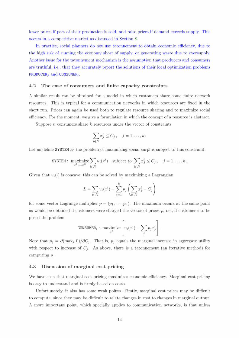
4.2 The case of consumers and finite capacity constraints

A similar result can be obtained for a model in which customers share some finite network

resources. This is typical for a communication networks in which resources are fixed in the

short run. Prices can again be used both to regulate resource sharing and to maximize social

efficiency. For the moment, we give a formulation in which the concept of a resource is abstract.

Suppose n consumers share k resources under the vector of constraints∑i∈N

xij ≤ Cj , j = 1, . . . , k .

Let us define SYSTEM as the problem of maximizing social surplus subject to this constraint:

SYSTEM : maximizex1,...,xn

∑i∈N

ui(xi) subject to∑i∈N

xij ≤ Cj , j = 1, . . . , k .

Given that ui(·) is concave, this can be solved by maximizing a Lagrangian

L =∑i∈N

ui(xi) −k∑

j=1

pj

(∑i∈N

xij − Cj

)

for some vector Lagrange multiplier p = (p1, . . . , pn). The maximum occurs at the same point

as would be obtained if customers were charged the vector of prices p, i.e., if customer i to be

posed the problem

CONSUMERi : maximizexi

ui(xi) −∑

j

pjxij

.

Note that pj = ∂(maxx L)/∂Cj . That is, pj equals the marginal increase in aggregate utility

with respect to increase of Cj . As above, there is a tatonnement (an iterative method) for

computing p .

4.3 Discussion of marginal cost pricing

We have seen that marginal cost pricing maximizes economic efficiency. Marginal cost pricing

is easy to understand and is firmly based on costs.

Unfortunately, it also has some weak points. Firstly, marginal cost prices may be difficult

to compute, since they may be difficult to relate changes in cost to changes in marginal output.

A more important point, which specially applies to communication networks, is that unless

14

marginal cost is appropriately defined, it can be either close to zero or to infinity. Think of

a telephone network that is built to carry C calls. When less than C calls are present the

short-run marginal cost of another call is near zero since the network already exists and its

cost (equipment and communication links) is a sunk cost; thus the extra cost that is incurred

by an extra call is negligible. On the other hand, when the network is critically loaded (all C

circuits are busy), then the cost of accommodating another call is huge. One has to expand the

network, and, in general, such expansion must take place in discrete steps, which involve large

costs (due to increasing transmission speed of the fibre, adding extra links, etc.). This means

that the short-run marginal cost of an extra call approaches infinity.

A proper definition of marginal cost should take account of the time frame over which the

network expands. The network can be considered to be continuously expanding (by averaging

the expansion that occurs in discrete steps), and the marginal cost of a circuit is then the

average cost of adding a circuit within this continuously expanding network. Thus marginal

cost could be interpreted as long-run average marginal cost.

Another difficulty in basing charges on marginal cost is that even if we know the marginal

cost and use it as a price, it can be difficult to predict the demand and to dimension the network

accordingly. There is a risk that we will build a network that is either too big or too small. A

pragmatic approach is to start conservatively and expand the network only if demand justifies

expansion. Prices are used to signal the need to expand the network. One starts with a small

network and adjusts prices so that demand equals the available capacity. If the prices required

to do this exceed the marginal cost of expanding the network, then additional capacity should

be built. Ideally, this process converges to a point, at which charges equal marginal cost and

the network is dimensioned optimally.

We should also bear in mind that the demand for network services tends to increase over

time. This also suggests that we should take a dynamic approach to setting prices and building

a network. If we dimension a network to operate reasonably over a period, then we might expect

that at the beginning of the period the network will be under utilized, while towards the end

of the period the demand will be larger than the network can accommodate. At this point, the

fact that high prices are required to limit the demand are a signal that it is time to expand the

network.

4.4 Recovering costs

Another weakness of marginal cost pricing is revealed when one considers that, in practice,

the supplier must recover his costs. In the case of a large firm operating under economies of

scale, the marginal cost is very small and the corresponding charge fails to recover the cost of

production. That is, social welfare is maximized at a point where π < 0, and so the supplier

does not recover his costs.

Two other methods by which a supplier can recover his costs while maximizing social wel-

fare are two-part tariffs and more general nonlinear prices. A typical two-part tariff is one in

15

which customers are charged both a fixed charge and a usage charge. Together these cover

the supplier’s reoccurring fixed costs and marginal costs. Note the difference between reoc-

curring fixed costs and non-reoccurring sunk costs. Sunk costs are those which have occurred

once-for-all. They can be included in the firm’s book as an asset, but they do not have any

bearing on the firm’s pricing decisions. For example, once a firm has already spent a certain

amount of money building a network, that amount becomes irrelevant to its pricing decisions.

Prices should be set to maximize profit, i.e., the difference between revenue and the costs of

production, both fixed and variable.

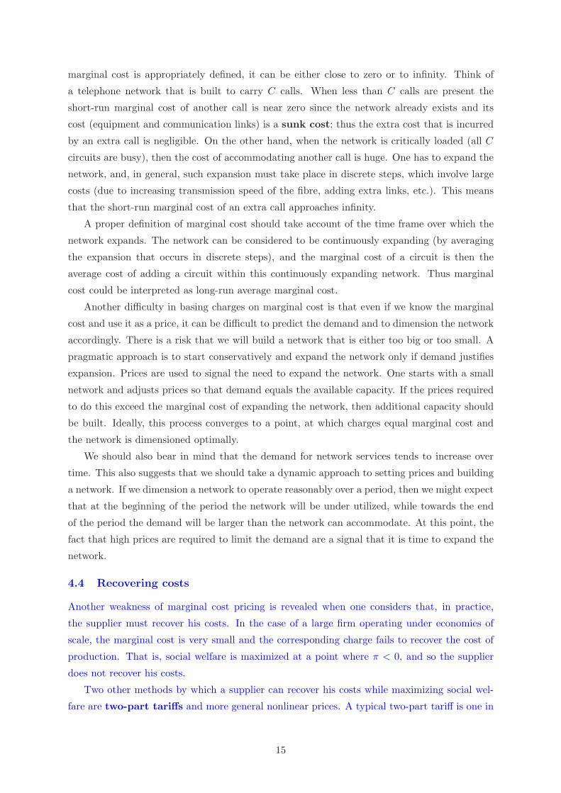
Suppose that the charge for a quantity x of a single service is set at a + px. The problem

for the consumer is to maximize his net benefit

u(x) − a − px .

He will choose x such that ∂u/∂x = p, unless his net benefit is negative at this point, in which

case it is optimal for him to take x = 0 and not participate. Thus a customer who buys a small

amount of the service if there is no fixed charge may be deterred from purchasing if a fixed

charge is made. This reduces social welfare, since although ‘large’ customers may purchase

their optimal quantities of the service, many ‘small’ customers may drop out and so obtain

no benefit. Observe that when p = MC, once a customer decides to participate, then he will

purchase the socially optimal amount.

pAC

MC

x

x(p)

x∗

$

MC

AC

F

Figure 4: In this example the marginal cost is constant and there is a linear demand function, x(p). Atwo part tariff recovers the additional amount F in the supplier’s cost by adding a fixed charge to theusage charge. Assuming N customers, the tariff may be F/N + xMC. However, a customer will notparticipate if his net benefit is negative. Observe that if the average cost curve AC = MC +F/x is usedto compute prices, then use of the resulting price pAC does not maximize social welfare. Average pricesare expected to have worse performance than two part tariffs using marginal cost prices.

How should one choose a and p? Choosing p = MC is definitely sensible, since this will

motivate socially optimal resource consumption. One can address the question of choosing a in

various ways. The critical issue is to motivate most of the customers to participate and so add

to the social surplus. If one knows the number of customers, then the simplest thing is to divide

16

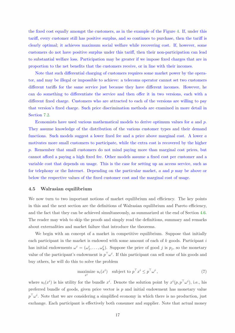
the fixed cost equally amongst the customers, as in the example of the Figure 4. If, under this

tariff, every customer still has positive surplus, and so continues to purchase, then the tariff is

clearly optimal; it achieves maximum social welfare while recovering cost. If, however, some

customers do not have positive surplus under this tariff, then their non-participation can lead

to substantial welfare loss. Participation may be greater if we impose fixed charges that are in

proportion to the net benefits that the customers receive, or in line with their incomes.

Note that such differential charging of customers requires some market power by the opera-

tor, and may be illegal or impossible to achieve: a telecoms operator cannot set two customers

different tariffs for the same service just because they have different incomes. However, he

can do something to differentiate the service and then offer it in two versions, each with a

different fixed charge. Customers who are attracted to each of the versions are willing to pay

that version’s fixed charge. Such price discrimination methods are examined in more detail in

Section 7.2.

Economists have used various mathematical models to derive optimum values for a and p.

They assume knowledge of the distribution of the various customer types and their demand

functions. Such models suggest a lower fixed fee and a price above marginal cost. A lower a

motivates more small customers to participate, while the extra cost is recovered by the higher

p. Remember that small customers do not mind paying more than marginal cost prices, but

cannot afford a paying a high fixed fee. Other models assume a fixed cost per customer and a

variable cost that depends on usage. This is the case for setting up an access service, such as

for telephony or the Internet. Depending on the particular market, a and p may be above or

below the respective values of the fixed customer cost and the marginal cost of usage.

4.5 Walrasian equilibrium

We now turn to two important notions of market equilibrium and efficiency. The key points

in this and the next section are the definitions of Walrasian equilibrium and Pareto efficiency,

and the fact that they can be achieved simultaneously, as summarized at the end of Section 4.6.

The reader may wish to skip the proofs and simply read the definitions, summary and remarks

about externalities and market failure that introduce the theorems.

We begin with an concept of a market in competitive equilibrium. Suppose that initially

each participant in the market is endowed with some amount of each of k goods. Participant i

has initial endowments ωi = (ωi1, . . . , ω

ik). Suppose the price of good j is pj , so the monetary

value of the participant’s endowment is p�ωi. If this participant can sell some of his goods and

buy others, he will do this to solve the problem

maximizexi

ui(xi) subject to p�xi ≤ p�ωi , (7)

where ui(xi) is his utility for the bundle xi. Denote the solution point by xi(p, p�ωi), i.e., his

preferred bundle of goods, given price vector is p and initial endowment has monetary value

p�ωi. Note that we are considering a simplified economy in which there is no production, just

exchange. Each participant is effectively both consumer and supplier. Note that actual money

17

may not be used. Prices express simple exchange rules between goods: if pi = kpj then one

unit of good i can be exchanged for k units of good j. Observe that (7) does not depend on

actual price scaling, but only on their relative values.

With xi = xi(p, p�ωi), we say that (x, p) is a Walrasian equilibrium from the initial

endowment ω = {ωij} if ∑

i

xi(p, p�ωi) ≤∑

i

ωi , (8)

that is, if there is no excess demand for any good when each participant buys the bundle

that is optimal for him given his budget constraint. It can be proved that for any initial

endowments ω there always exists a Walrasian equilibrium for some price vector p. That is,

there is some p at which markets clear. In fact, this p can be found by a tatonnement mechanism.

The Walrasian equilibrium is also called a competitive equilibrium, since it is reached as

participants compete for goods, which become allocated to those participants who value them

most (formally, economists call a market competitive if all firms are price takers). Throughout

the following we assume that all utilities are increasing and concave, so that p is certainly

nonnegative and the inequalities in (7) and (8) are sure to be equalities at the equilibrium.

Equivalently, under this assumption, (x, p) is a Walrasian equilibrium if

(1)∑

i

xi =∑

i

ωi ,

(2) If xi is preferred by participant i to xi, then p�xi > p�xi .

4.6 Pareto efficiency

We now relate the idea of Walrasian equilibrium to another solution concept, that of Pareto

efficiency. We say that a solution point (an allocation of goods to participants) is Pareto

efficient if there is no other point for which all participants are at least as well off and at least

one participant is strictly better off, for the same total amounts of the goods. In other words, it

is not possible to make one participant better off without making at least one other participant

worse off. Mathematically, we say as follows.

The allocation x1, . . . , xn is not Pareto efficient ifthere exists x1, . . . , xn, with

∑i x

i =∑

i xi,

such that ui(xi) ≥ ui(xi) for every i,and at least one of these inequalities is strict.

(9)

Unlike social welfare, Pareto efficiency is not concerned with the sum of the participants’ utilities.

Instead, it characterizes allocations which cannot be strictly improved ‘componentwise’. In the

following two theorems we see that Walrasian equilibria can be equated with Pareto efficient

points. We assume that the utility functions are strictly increasing and concave and there are

no market failures. The following theorem says that a market economy will achieve a Pareto

efficient result. It holds under the assumption that (7) is truly the problem faced by participant

i. In particular, this means that his utility must depend only the amounts of the goods he holds,

not the amounts held by others or their utilities. So there must be no unpriced externalities

18

or information asymmetries. These mean there are missing markets (things unpriced), and

so-called market failure.

Theorem 1 (first theorem of welfare economics) If (x, p) is a Walrasian equilibrium then

it is Pareto efficient.

Theorem 2 (second theorem of welfare economics) Suppose ω is a Pareto efficient al-

location in which ωij > 0 for all i, j. Then there exists a p such that (ω, p) is a Walrasian

equilibrium from any initial endowment ω such that∑

i ωi =

∑i ω

i, and p�ωi = p�ωi for all i.

Notice that, given any initial endowment ω such that∑

i ωi =

∑i ω

i, i.e., ω and ω contain

the same total quantity of each good, we can support a Pareto efficient ω as the Walrasian

equilibrium if we are allowed to first make a lump sum redistribution of the endowments. We

can do this by redistributing the initial endowments ω to any ω, such that p�ωi = p�ωi for all

i. Of course, this can be done trivially by taking ω = ω, but other ω may be easier to achieve in

practice. For example, we might find it difficult to redistribute a good called ‘labour’. If there

is a good called ‘money’, then we can do everything by redistributing that good alone, i.e., by

subsidy and taxation.

Let us now return to the problem of social welfare maximization:

maximizex

∑i

ui(xi) , subject to∑

i

xij ≤ ωj for all j. (10)

For ωj = Cj this is the problem of Section 4.2. We can make the following statement about its

solution.

Theorem 3 Every social welfare optimum is Pareto efficient.

One can extend the above theorem for more general definitions of the social welfare function

W (u1(x1), . . . , un(xn)), where we only require that W is increasing in each of its arguments.

Fro instance, we could define

W (u1(x1), . . . , un(xn)) =∑

i

aiui(xi) , (11)

for positive weights ai.

Finally, note that we can cast the welfare maximization problem of Section 4.1 into the above

form (i.e., welfare maximization with resource constraints), if we imagine that the producer is

participant 1, and the set of consumers is N = {2, . . . , n}. Define for the producer its utility

function u1(x1) = −c(ω1−x1), for some appropriately large vector of every good ω, noting that

this is a concave increasing function of x1 if c is convex increasing. Now the the constraint in

(10) is x1 +∑

i∈N xi ≤ ω1, and the optimum we will have x1 +∑

i∈N xi = ω1. Thus, (10) is

simply

maximizex2,...,xn

∑i∈N

ui(xi) − c

(∑i∈N

xi

).

19

Therefore we can also conclude that for this model with a producer, the same conclusions

regarding pareto efficiency hold.

In summary, these conclusion are that there is a set of relationships between welfare maxima,

competitive equilibria and Pareto efficient allocations:

1. competitive equilibria are Pareto efficient;

2. Pareto efficient allocations are competitive equilibria for some initial endowments;

3. welfare maxima are Pareto efficient;

4. Every Pareto efficient allocation is social welfare optimal for some appropriate social

welfare function (by choosing the coefficients ai in (11)).

The importance of these results is to show that various reasonable notions of what constitutes

‘optimal production and consumption in the market’ are consistent with one another. It can

be found by a social planner who control prices to maximize social welfare, or by the ‘invisible

hand’ of the market, which acts as participants individually seeking to maximize their own

utilities.

5 Network externalities

Throughout this chapter we have supposed that a customer’s utility depends only on the goods

that he himself consumes. This is not true when goods exhibit network externalities, i.e., when

they become more valuable as more customers use them. Examples of such goods are telephones,

fax machines, and computers connected to the Internet. Let us analyze a simple model to see

what can happen.

Suppose there are N potential customers, indexed by i = 1, . . . , N , and that customer i is

willing to pay ui(n) = ni for a unit of the good, given that n other customers will be using

it. Thus, if a customer believes that no one else will purchase the good, he values it at zero.

Assume also that a customer who purchases the good can always return it for a refund if he

detects that it is worth less to him that the price he paid. We will compute the demand curve

in such a market, i.e., given a price p for a unit of the good, the number of customers who will

purchase it. Suppose that p is posted and n customers purchase the good. We can think of n

as an equilibrium point in the following way: n customers have taken the risk of purchasing

the good (say by having a strong prior belief that n − 1 other customers will also purchase

it), and at that point no new customer wants to purchase the good, and no existing purchaser

wants to return it, so that n is stable for the given p. Clearly, the purchasers will be customers

N − n + 1, . . . , N . Since there are more customers that do not think it is profitable in this

situation to purchase the good, there must be such an ‘indifferent’ customer, for which the

value of the good equals the price. This should be customer i = N − n, and since ui(n) = p we

obtain that the demand at price p is that n such that n(N −n) = p. Note that in general there

are two values of n for which this holds. E.g., for N = 100 and p = 1600, n can be 20 or 80.

20

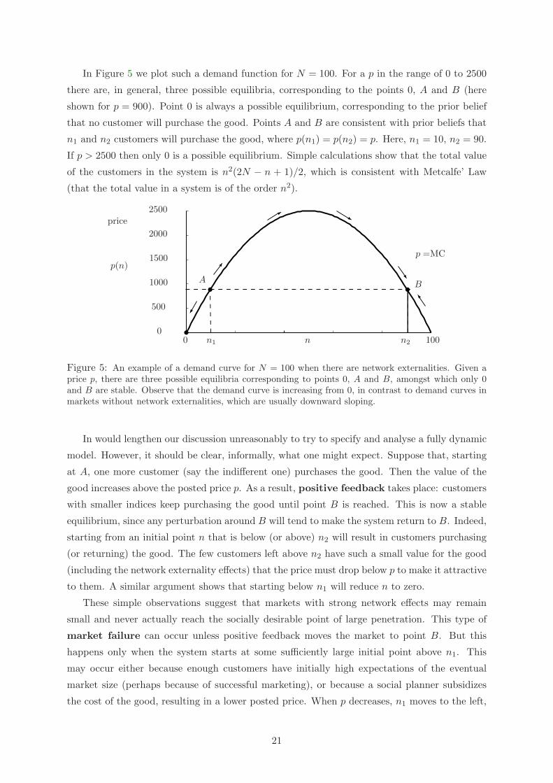
In Figure 5 we plot such a demand function for N = 100. For a p in the range of 0 to 2500

there are, in general, three possible equilibria, corresponding to the points 0, A and B (here

shown for p = 900). Point 0 is always a possible equilibrium, corresponding to the prior belief

that no customer will purchase the good. Points A and B are consistent with prior beliefs that

n1 and n2 customers will purchase the good, where p(n1) = p(n2) = p. Here, n1 = 10, n2 = 90.

If p > 2500 then only 0 is a possible equilibrium. Simple calculations show that the total value

of the customers in the system is n2(2N − n + 1)/2, which is consistent with Metcalfe’ Law

(that the total value in a system is of the order n2).

2500

2000

1500

500

100

1000

00

AB

n1 n2n

p =MCp(n)

price

Figure 5: An example of a demand curve for N = 100 when there are network externalities. Given aprice p, there are three possible equilibria corresponding to points 0, A and B, amongst which only 0and B are stable. Observe that the demand curve is increasing from 0, in contrast to demand curves inmarkets without network externalities, which are usually downward sloping.

In would lengthen our discussion unreasonably to try to specify and analyse a fully dynamic

model. However, it should be clear, informally, what one might expect. Suppose that, starting

at A, one more customer (say the indifferent one) purchases the good. Then the value of the

good increases above the posted price p. As a result, positive feedback takes place: customers

with smaller indices keep purchasing the good until point B is reached. This is now a stable

equilibrium, since any perturbation around B will tend to make the system return to B. Indeed,

starting from an initial point n that is below (or above) n2 will result in customers purchasing

(or returning) the good. The few customers left above n2 have such a small value for the good

(including the network externality effects) that the price must drop below p to make it attractive

to them. A similar argument shows that starting below n1 will reduce n to zero.

These simple observations suggest that markets with strong network effects may remain

small and never actually reach the socially desirable point of large penetration. This type of

market failure can occur unless positive feedback moves the market to point B. But this

happens only when the system starts at some sufficiently large initial point above n1. This

may occur either because enough customers have initially high expectations of the eventual

market size (perhaps because of successful marketing), or because a social planner subsidizes

the cost of the good, resulting in a lower posted price. When p decreases, n1 moves to the left,

21

making it possible grow the customer base from a smaller initial value. Thus it may be sensible

to subsidize the price initially, until positive feedback takes place. Once the system reaches a

stable equilibrium one can raise prices or use some other means to pay back the subsidy.

These conditions are frequently encountered in the communications market. For instance,

the wide penetration of broadband information services requires low prices for access services

(access the Internet with speeds higher than a few Mbps). But prices will be low for access once

enough demand for broadband attracts more competition in the provision of such services and

motivates the development and deployment of more cost-effective access technologies. This is a

typical case of the traditional ‘chicken and egg’ problem!

Finally, we make an observation about social welfare maximization. Suppose that in our

example with N = 100, the marginal cost of the good is p. If we compute the social welfare

S(n), it turns out that its derivative is positive at n2 for any p that intersects the demand curve,

and remains positive until N is reached. Hence it is socially optimal to consume even more than

the equilibrium quantity n2. In this case, marginal cost pricing is not optimal, the optimal price

being zero. This suggests that when strong network externalities are present, optimal pricing

may be below marginal cost, in which case the social planer should subsidize the price of the

good that creates these externalities. Such a subsidy could be recovered from the customers’

surplus by taxation.

6 Types of competition

The market in which suppliers and customers interact can be extraordinarily complex. Each

participant seeks to maximize his own surplus. Different actions, information and market power

are available to the different participants. One imagines that a large number of complex games

can take place as they compete for profit and consumer surplus. The following sections are

concerned with three basic models of market structure and competition: monopoly, perfect

competition and oligopoly.

In a monopoly there is a single supplier who controls the amount of goods produced. In

practice, markets with a single supplier tend to arise when the goods have a production function

that exhibits the properties of a natural monopoly. A market is said to be a natural monopoly

if a single supplier can always supply the aggregate output of several smaller suppliers at less

than the total of their costs. This is due both to production economies of scale (the average

cost of production decreases with the quantity of a good produced) and economies of scope

(the average cost of production decreases with the number of different goods produced). Mathe-

matically, if all suppliers share a common cost function, c, this implies c(x+y) ≤ c(x)+c(y), for

all vector quantities of services x and y. We say that c(·) is a subadditive function. This is

frequently the case when producing digital goods, where there is some fixed initial development

cost and nearly zero cost to reproduce and distribute through the Internet.

In such circumstances a larger supplier can set prices below those of smaller competitors

and so capture the entire market for himself. Once the market is his alone then his problem

22

is essentially one of profit maximization. In Section 7 we show that a monopolist maximizes

his profit (surplus) by taking account of the customers’ price elasticities. He can benefit by

discriminating amongst customers with different price elasticities or preferences for different

services. His monopoly position allows him to maximize his surplus while reducing the surplus

of the consumers. If he can discriminate perfectly between customers, then he can make a

take-it-or-leave it offer to each customer, thereby maximizing social welfare, but keeping all of

its value for himself. If he can only imperfectly discriminate, then the social welfare will be

less than maximal. Intuitively, the monopolist keeps prices higher than socially optimal, and

reduces demand while increasing his own profit.

Monopoly is not necessarily a bad thing. Society as a whole can benefit from the large pro-

duction economies of scale that a single firm can achieve. Incompatibilities amongst standards,

and the differing technologies with which disparate suppliers might provide a service, can reduce

that service’s value to customers. This problem is eliminated when a monopolist sets a single

standard. This is the main reason that governments often support monopolies in sectors of the

economy such as telecommunications and electric power generation. The government regulates

the monopoly’s prices, allowing it to recover costs and make a reasonable profit. Prices are kept

close to marginal cost and social welfare is almost maximized. However, there is the danger

that such a ‘benevolent’ monopoly does not have much incentive to innovate.

A price reduction of a few percent may be insignificant compared with the increase of social

value that can be obtained by the introduction of completely new and life-changing services.

This is especially so in the field of communications services. A innovation is much more likely

to occur in the context of a competitive market.

A second competition model is perfect competition. The idea is that there are many suppliers

and consumers in the market, every such participant in the market is small and so no individual

consumer or supplier can dictate prices. All participants are price-takers. Consumers solve

a problem of maximizing net surplus, by choice of the amounts they buy. Suppliers solve a

problem of maximizing profit, by choice of the amounts they supply. Prices naturally gravitate

towards a point where demand equals supply. The key result in Section 8 is that at this point

the social surplus is maximized, just as it would be if there were a regulator and prices were set

equal to marginal cost. Thus perfect competition is an ‘invisible hand’ that produces economic

efficiency. However, perfect competition is not always easy to achieve. As we have noted there

can be circumstances in which monopoly is preferable.

In practice, many markets consist of only a few suppliers. Oligopoly is the name given to

such a market. As we see in Section 9 there are a number of games that one can use to model

such circumstances. The key results of this section are that the resulting prices are sensitive to

the particular game formulation, and hence depend on modelling assumptions. In a practical

sense, prices in an oligopoly lie between two extremes: these imposed by a monopolist and

those obtained in a perfectly competitive market. The greater the number of producers and

consumers, the greater will be the degree of competition and hence the closer prices will be to

23

those that arise under perfect competition.

We have mentioned that if supply to a market has large production economies of scale, then

a single supplier is likely to dominate eventually. This market organization of ‘winner-takes-all’

is all the more likely if there are network externality effects, i.e., if there are economies of scale

in demand. The monopolist will tend to grow, and will take advantages of economies of scope

to offer more and more services.

7 Monopoly

7.1 Profit maximization

A monopoly supplier has the problem of profit maximization. Since he is the only supplier

of the given goods, he is free to choose prices. In general, such (unit) prices may be different

depending on the amount sold to a customer, and may also depend on the identity of the

customer. Such a flexibility in defining prices may not be available in all market situations.

For instance, at a retail petrol station, the price per litre is the same for all customers and

independent of the quantity they purchase. In contrast, a service provider can personalize

the price of a digital good, or of a communications service, by taking account of any given

customer’s previous history or special needs to create a version of the service that he alone may

use. Sometimes quantity discounts can be offered. As we see below, the more control that a

firm has to discriminate and price according to the identity of the customer or the quantity he

purchases, the more profit it can make. Before investigating three types of price discrimination,

we start with the simplest case, in which the monopolist is allowed to use only linear prices,

(i.e., the same for all units), uniform across customers.

Let xj(p) denote the demand for service j when the price vector for a set of services is p.

A monopoly supplier whose goal is profit maximization will choose to post prices that solve

the problem

maximizep

∑j

pjxj(p) − c(x)

.

The first-order stationarity condition with respect to pi is

xi +∑

j

pj∂xj

∂pi−

∑j

∂c

∂xj

∂xj

∂pi= 0 . (12)

If services are independent (so that εij = 0 for i �= j), we have

pi

(1 +

1εi

)=

∂c

∂xi.

One can check that this is equivalent to saying that marginal revenue should equal marginal

cost. This condition is intuitive, since if marginal revenue were greater (or less) than marginal

cost, then the monopolist could increase his profit by adjusting the price so that the demand

increased (or decreased). Recall that marginal cost prices maximize social welfare. Since εi < 0

the monopolist sets a price for service i that is greater than his marginal cost ∂c(x)/∂xi. At

24

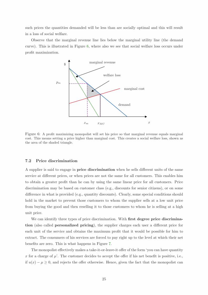
such prices the quantities demanded will be less than are socially optimal and this will result

in a loss of social welfare.

Observe that the marginal revenue line lies below the marginal utility line (the demand

curve). This is illustrated in Figure 6, where also we see that social welfare loss occurs under

profit maximization.

welfare loss

marginal revenue

demand

$

xm xMC

pm

x

marginal cost

Figure 6: A profit maximizing monopolist will set his price so that marginal revenue equals marginalcost. This means setting a price higher than marginal cost. This creates a social welfare loss, shown asthe area of the shaded triangle.

7.2 Price discrimination

A supplier is said to engage in price discrimination when he sells different units of the same

service at different prices, or when prices are not the same for all customers. This enables him

to obtain a greater profit than he can by using the same linear price for all customers. Price

discrimination may be based on customer class (e.g., discounts for senior citizens), or on some

difference in what is provided (e.g., quantity discounts). Clearly, some special conditions should

hold in the market to prevent those customers to whom the supplier sells at a low unit price

from buying the good and then reselling it to those customers to whom he is selling at a high

unit price.

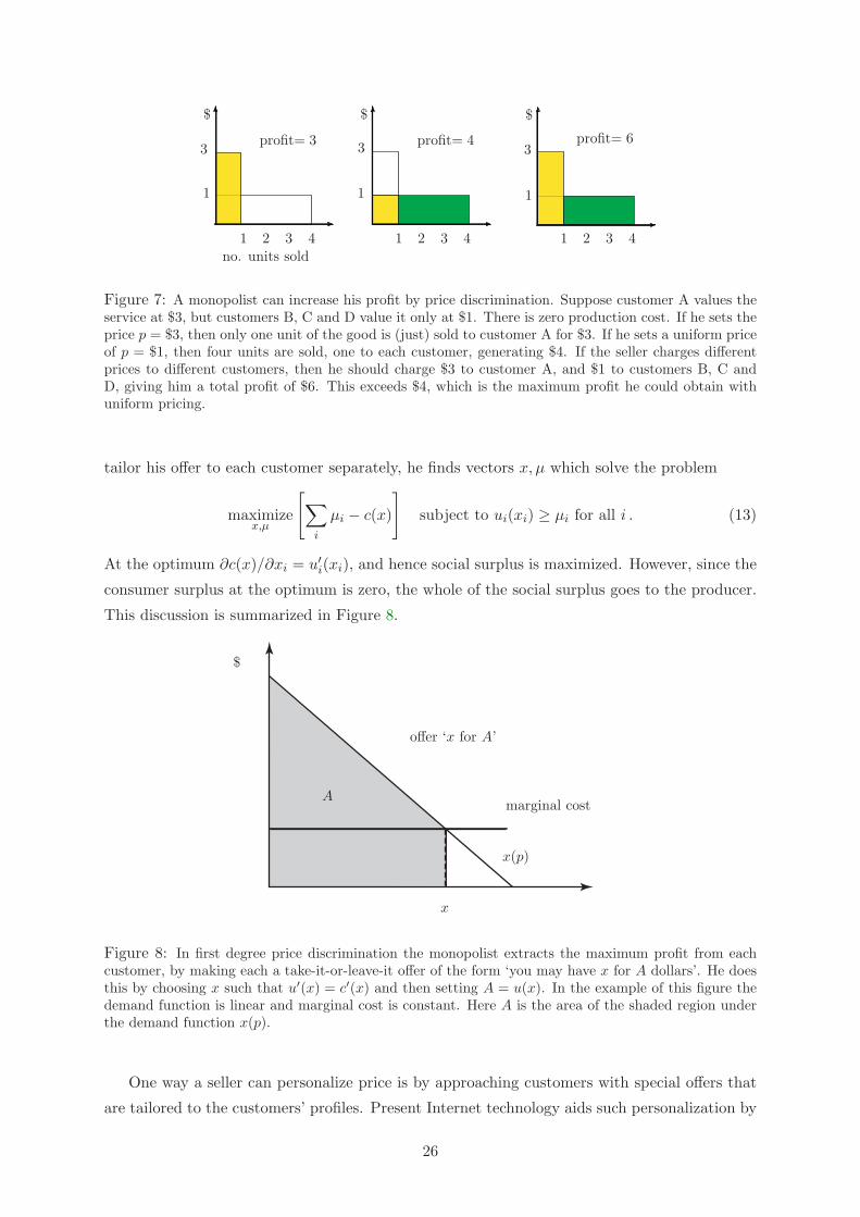
We can identify three types of price discrimination. With first degree price discrimina-

tion (also called personalized pricing), the supplier charges each user a different price for

each unit of the service and obtains the maximum profit that it would be possible for him to

extract. The consumers of his services are forced to pay right up to the level at which their net

benefits are zero. This is what happens in Figure 7.

The monopolist effectively makes a take-it-or-leave-it offer of the form ‘you can have quantity

x for a charge of µ’. The customer decides to accept the offer if his net benefit is positive, i.e.,

if u(x) − µ ≥ 0, and rejects the offer otherwise. Hence, given the fact that the monopolist can

25

$ $ $

111

1 1 1

222 333

3 3 3

444

profit= 3 profit= 4 profit= 6

no. units sold

Figure 7: A monopolist can increase his profit by price discrimination. Suppose customer A values theservice at $3, but customers B, C and D value it only at $1. There is zero production cost. If he sets theprice p = $3, then only one unit of the good is (just) sold to customer A for $3. If he sets a uniform priceof p = $1, then four units are sold, one to each customer, generating $4. If the seller charges differentprices to different customers, then he should charge $3 to customer A, and $1 to customers B, C andD, giving him a total profit of $6. This exceeds $4, which is the maximum profit he could obtain withuniform pricing.

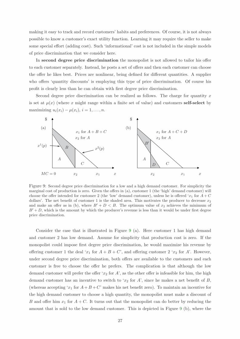
tailor his offer to each customer separately, he finds vectors x, µ which solve the problem

maximizex,µ

[∑i

µi − c(x)

]subject to ui(xi) ≥ µi for all i . (13)

At the optimum ∂c(x)/∂xi = u′i(xi), and hence social surplus is maximized. However, since the

consumer surplus at the optimum is zero, the whole of the social surplus goes to the producer.

This discussion is summarized in Figure 8.

marginal cost

x(p)

x

offer ‘x for A’

$

A

Figure 8: In first degree price discrimination the monopolist extracts the maximum profit from eachcustomer, by making each a take-it-or-leave-it offer of the form ‘you may have x for A dollars’. He doesthis by choosing x such that u′(x) = c′(x) and then setting A = u(x). In the example of this figure thedemand function is linear and marginal cost is constant. Here A is the area of the shaded region underthe demand function x(p).

One way a seller can personalize price is by approaching customers with special offers that

are tailored to the customers’ profiles. Present Internet technology aids such personalization by

26

making it easy to track and record customers’ habits and preferences. Of course, it is not always

possible to know a customer’s exact utility function. Learning it may require the seller to make

some special effort (adding cost). Such ‘informational’ cost is not included in the simple models

of price discrimination that we consider here.

In second degree price discrimination the monopolist is not allowed to tailor his offer

to each customer separately. Instead, he posts a set of offers and then each customer can choose

the offer he likes best. Prices are nonlinear, being defined for different quantities. A supplier

who offers ‘quantity discounts’ is employing this type of price discrimination. Of course his

profit is clearly less than he can obtain with first degree price discrimination.

Second degree price discrimination can be realized as follows. The charge for quantity x

is set at µ(x) (where x might range within a finite set of value) and customers self-select by

maximizing ui(xi) − µ(xi), i = 1, . . . , n.

$ $

(a) (b)

AA

BB′

CC D

x1x1 x2x2

x1(p)x2(p)

xx

x2 for Ax2 for A

x1 for A + B + C x1 for A + C + D

MC = 0

Figure 9: Second degree price discrimination for a low and a high demand customer. For simplicity themarginal cost of production is zero. Given the offers in (a), customer 1 (the ‘high’ demand customer) willchoose the offer intended for customer 2 (the ‘low’ demand customer), unless he is offered ‘x1 for A + Cdollars’. The net benefit of customer 1 is the shaded area. This motivates the producer to decrease x2

and make an offer as in (b), where B′ + D < B. The optimum value of x2 achieves the minimum ofB′ + D, which is the amount by which the producer’s revenue is less than it would be under first degreeprice discrimination.

Consider the case that is illustrated in Figure 9 (a). Here customer 1 has high demand

and customer 2 has low demand. Assume for simplicity that production cost is zero. If the

monopolist could impose first degree price discrimination, he would maximize his revenue by

offering customer 1 the deal ‘x1 for A + B + C’, and offering customer 2 ‘x2 for A’. However,

under second degree price discrimination, both offers are available to the customers and each

customer is free to choose the offer he prefers. The complication is that although the low

demand customer will prefer the offer ‘x2 for A’, as the other offer is infeasible for him, the high

demand customer has an incentive to switch to ‘x2 for A’, since he makes a net benefit of B,

(whereas accepting ‘x1 for A+B +C’ makes his net benefit zero). To maintain an incentive for

the high demand customer to choose a high quantity, the monopolist must make a discount of

B and offer him x1 for A + C. It turns out that the monopolist can do better by reducing the

amount that is sold to the low demand customer. This is depicted in Figure 9 (b), where the

27

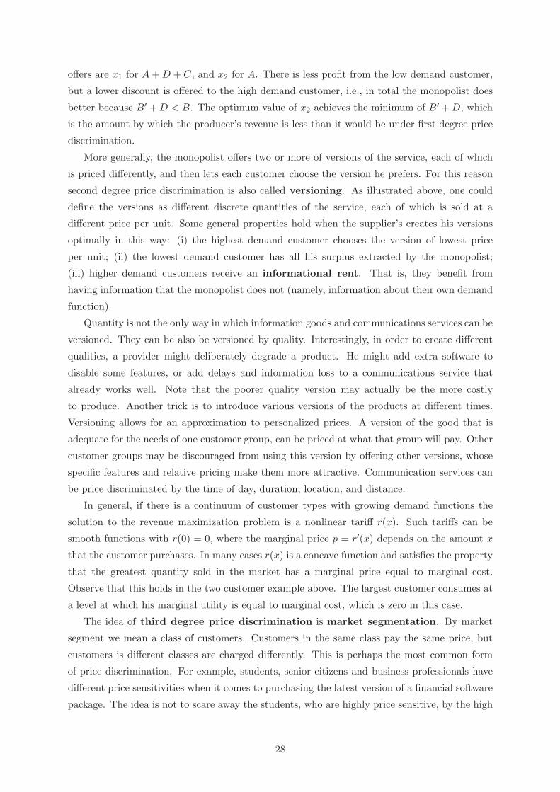
offers are x1 for A + D + C, and x2 for A. There is less profit from the low demand customer,

but a lower discount is offered to the high demand customer, i.e., in total the monopolist does

better because B′ + D < B. The optimum value of x2 achieves the minimum of B′ + D, which

is the amount by which the producer’s revenue is less than it would be under first degree price

discrimination.

More generally, the monopolist offers two or more of versions of the service, each of which

is priced differently, and then lets each customer choose the version he prefers. For this reason

second degree price discrimination is also called versioning. As illustrated above, one could

define the versions as different discrete quantities of the service, each of which is sold at a

different price per unit. Some general properties hold when the supplier’s creates his versions

optimally in this way: (i) the highest demand customer chooses the version of lowest price

per unit; (ii) the lowest demand customer has all his surplus extracted by the monopolist;

(iii) higher demand customers receive an informational rent. That is, they benefit from

having information that the monopolist does not (namely, information about their own demand

function).

Quantity is not the only way in which information goods and communications services can be

versioned. They can be also be versioned by quality. Interestingly, in order to create different

qualities, a provider might deliberately degrade a product. He might add extra software to

disable some features, or add delays and information loss to a communications service that

already works well. Note that the poorer quality version may actually be the more costly

to produce. Another trick is to introduce various versions of the products at different times.

Versioning allows for an approximation to personalized prices. A version of the good that is

adequate for the needs of one customer group, can be priced at what that group will pay. Other

customer groups may be discouraged from using this version by offering other versions, whose

specific features and relative pricing make them more attractive. Communication services can

be price discriminated by the time of day, duration, location, and distance.

In general, if there is a continuum of customer types with growing demand functions the

solution to the revenue maximization problem is a nonlinear tariff r(x). Such tariffs can be

smooth functions with r(0) = 0, where the marginal price p = r′(x) depends on the amount x

that the customer purchases. In many cases r(x) is a concave function and satisfies the property

that the greatest quantity sold in the market has a marginal price equal to marginal cost.

Observe that this holds in the two customer example above. The largest customer consumes at

a level at which his marginal utility is equal to marginal cost, which is zero in this case.

The idea of third degree price discrimination is market segmentation. By market

segment we mean a class of customers. Customers in the same class pay the same price, but

customers is different classes are charged differently. This is perhaps the most common form

of price discrimination. For example, students, senior citizens and business professionals have

different price sensitivities when it comes to purchasing the latest version of a financial software

package. The idea is not to scare away the students, who are highly price sensitive, by the high

28

prices that one can charge to the business customers, who are price insensitive. Hence, one

could use different prices for different customer groups (the market segments). Of course, the

seller of the services must have a way to differentiate customers that belong to different groups

(for example, by requiring sight of a student id card). This explains why third degree price

discrimination is also called group pricing.

Suppose that customers in class i have a demand function of xi(p) for some service. The

monopolist seeks to maximize

max{xi(·)}

n∑i=1

pixi(pi) − c

(n∑

i=1

xi(pi)

).

Assuming for simplicity that the market segments corresponding to the different classes are

completely separated, the first order conditions are

pi(xi) + p′i(xi)xi = c′(

n∑i=1

xi

).

If εi is the demand elasticity in market i, then these conditions can be written as

pi(xi)(

1 +1εi

)= c′

(n∑

i=1

xi

). (14)

These results are intuitive. The monopolist will charge the lowest price to the market segment

that has the greatest demand elasticity. In Figure 10 there are two customers classes, with

demand functions x1(p) = 6− 3p and x2(p) = 2− 2p. The solution to (14) with the right hand

side equal to 1/2 is p1 = 5/4 and p2 = 3/4, with x1 = 9/2 and x2 = 1/4. At these points,

ε1 = −5/3, ε2 = −3.

The market segment that is most price inelastic will be charged the highest price. Similar

results hold when the markets are not independent and prices influence demand across markets.

A simple but clever way to implement group pricing is through discount coupons. The

service is offered at a discount price to customers with coupons. It is time consuming to collect

coupons. One class of customers is prepared to put in the time and another is not. The

customers are effectively divided into two groups by their price elasticity. Those with a greater

price elasticity will collect coupons and end up paying a lower price.

It is interesting to ask whether or not the overall economy benefits from third degree price

discrimination. The answer is that it can go either way. Price discrimination can only take place

if different consumers have unequal marginal utilities at their levels of consumption, which is

(generally) bad for welfare. But it can increase consumption, which is good for welfare. A

necessary condition for there to be an increase in welfare is that there should be an increase in

consumption. This happens in the example of Figure 10. There are two markets and one is much

smaller than the other. If third degree price discrimination is not allowed, then the monopolist

will charge a high price and this will discourage participation from the small market. However,

if third degree price discrimination is allowed, he can set the same price for the high demand

market, and set a low price for the low demand market, so that this market now participates. If

29

$

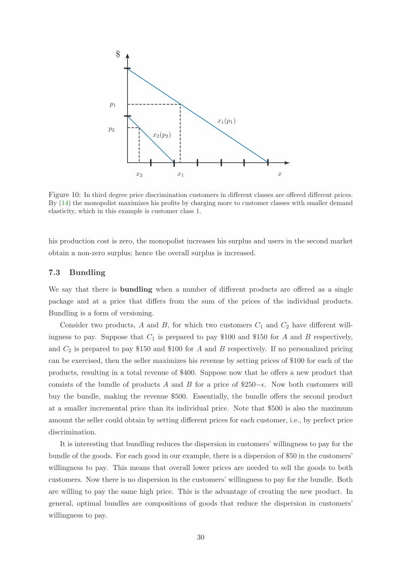
x1x2

p1

p2

x

x1(p1)

x2(p2)

Figure 10: In third degree price discrimination customers in different classes are offered different prices.By (14) the monopolist maximizes his profits by charging more to customer classes with smaller demandelasticity, which in this example is customer class 1.

his production cost is zero, the monopolist increases his surplus and users in the second market

obtain a non-zero surplus; hence the overall surplus is increased.

7.3 Bundling

We say that there is bundling when a number of different products are offered as a single

package and at a price that differs from the sum of the prices of the individual products.

Bundling is a form of versioning.

Consider two products, A and B, for which two customers C1 and C2 have different will-

ingness to pay. Suppose that C1 is prepared to pay $100 and $150 for A and B respectively,

and C2 is prepared to pay $150 and $100 for A and B respectively. If no personalized pricing

can be exercised, then the seller maximizes his revenue by setting prices of $100 for each of the

products, resulting in a total revenue of $400. Suppose now that he offers a new product that

consists of the bundle of products A and B for a price of $250−ε. Now both customers will

buy the bundle, making the revenue $500. Essentially, the bundle offers the second product

at a smaller incremental price than its individual price. Note that $500 is also the maximum

amount the seller could obtain by setting different prices for each customer, i.e., by perfect price

discrimination.

It is interesting that bundling reduces the dispersion in customers’ willingness to pay for the

bundle of the goods. For each good in our example, there is a dispersion of $50 in the customers’

willingness to pay. This means that overall lower prices are needed to sell the goods to both

customers. Now there is no dispersion in the customers’ willingness to pay for the bundle. Both

are willing to pay the same high price. This is the advantage of creating the new product. In

general, optimal bundles are compositions of goods that reduce the dispersion in customers’

willingness to pay.

30

Bundling is common in the service offerings of communication providers. For instance, it

is usual for an ISP to charge its subscribers a monthly flat fee that includes an email account,

the hosting of a web page, some amount of on-line time, permission to download some quantity

of data, messaging services, and so on. If each service were priced individually, there would be

substantial dispersion in the users’ willingness to pay. By creating a bundle, the service provider

decreases the dispersion in pay and can obtain a greater revenue.

7.4 Service differentiation and market segmentation

We have discussed the notion of market segmentation, in which the monopolist is able to set

different prices for his output in different markets. But can the monopolist always segment the

market in this way? In many realistic situations there is nothing to prevent the customers of

one market from buying in another market. However, sometimes the monopolist can construct

a barrier to prevent this. As we have said, he might sell discounted tickets to students, but

require proof of student status.

One way to create market segmentation is by service differentiation. This is accomplished

by producing versions of a service that are not fully substitutable for one another. Each service

is specialized for the target market segment. For example think of a company that produces

alcohol. The markets consist of customers that use alcohol as a pharmaceutical ingredient and

customers that use it in lamps for lighting. In order to segment the market, the manufacturer

might add a chemical adulterant to the alcohol that prevents its use as a pharmaceutical. If this

market is the least price-elastic, then he will be able to charge a higher price for the pure alcohol

that for the alcohol sold for lamps. Note that the marginal cost of producing the products is

nearly the same. The lamp alcohol might actually be a bit more expensive, since it involves

addition of the adulterant.

This type of price discrimination is popular in the communications market. The network

operator posts a list of services and tariffs and customers are free to choose the service-tariff

pair they like better. Versioning of communication services requires care and must take account

of substitution effects such as arbitrage and traffic splitting. Arbitrage occurs when a customer

can make a profit by buying a service of a certain type and then repackaging and reselling it as

a different service at market prices. For instance, if the price of a 2 Mbps connection is less than

twice the price of a 1 Mbps connection, then there may be a business opportunity for a customer

to buy a number of 2 Mbps connections and become a supplier of 1 Mbps connections at lower

prices. Unless there is a substantial cost in reselling bandwidth, such a pricing scheme has

serious flaws since no one will ever wish directly to buy a 1 Mbps connection. A similar danger

can arise from traffic splitting. This takes place when a user splits a service into smaller services,

and pays less this way than if he had bought the smaller services at market prices. In our simple

example, the price of a popular 2 Mbps service could be much higher than twise the price of 1

Mbps services. In general, there is cost to first splitting and then later reconstructing the initial

traffic. One must take these issues into account when constructing prices for service contracts.

31

Finally, we remark upon the role of content in price discrimination. Usually, it is practically

impossible to make prices depend on the particular content that a network connection carries,

for instance, to differently price the transport of financial data and leisure content. The network

operator is usually not allowed to read the information that his customers send. In any case,

data can be encrypted at the application layer. This means that it is usually not possible to

price discriminate on the basis of content.

In general, service contracts are characterized by more parameters than just the peak rate,

such as the mean rate and burstiness. This weakens the substitution effects since it is not always

clear how to combine or split contracts with arbitrary parameters. But the most effective way

to prevent substitution is by quality of service differentiation. Consider a simple example. A

supplier might offer two services, one with small delay and losses, and one with greater delay.

This will divide the market into two segments. One segment consists of users who need high

quality video and multimedia services. The other consists of users who need only e-mail and web

browsing. Depending on the difference in the two market’s demand elasticities, the prices that

the supplier can charge per unit of bandwidth can differ by orders of magnitude, even though

the marginal costs of production might be nearly the same. Even if the supplier can provide

the lower quality services at a quality that is not too different from the high quality ones, it

can be to his benefit artificially to degrade the lower quality service, in order to maintain a

segmentation of the market and retain the revenue of customers in the first market, who might

otherwise be content with the cheaper service.

How about the consumer? Can he benefit from service differentiation, or is it only a means

for a profit-seeking producer to increase his profit? The answer is that it depends. A good rule of

thumb is to look at the change in the quantity of services consumed. If the introduction of new

versions of a service stimulates demand and creates new markets, then both consumer surplus

and producer surplus are probably increased. The existence of more versions of service helps

consumers express their true needs and preferences, and increases their net benefits. However,

the cost of differentiating services must be offset against this.

In networks, service differentiation is often achieved by giving some customers priority, or

reserving resources for them. What makes the problem hard is that the service provider cannot

completely define the versions of the services a priori, since quality factors may depend on the

numbers of customers who end up subscribing for the services.

8 Perfect competition

We have discussed the case of a market that is in the control of a profit-seeking monopolist.

The job of a regulator is to obtain for the market the benefits of the monopolist’s low costs of

production, but while maximizing social surplus. A regulator could impose prices in a market

with the aim of maximizing social surplus, subject to suppliers being allowed to make certain

profits. However, regulation can be costly and imperfect. It may also be difficult for a regulator

to encourage a monopolist to innovate and to offer new services and products. Interestingly,

32

the goals of the regulator can be achieved by increasing the competition in the market.

If there is no supplier or customer in the market who is so dominant that he can dictate prices,

then social surplus can still be maximized, but by the effect of perfect competition. Every

participant in the market is small. As a consequence he assumes that prices are determined by

the market and cannot be influenced by any of his decisions, i.e., he is a price taker. Consumer

i solves a problem of maximizing his net surplus, by demanding xi, where ∂ui(xi)/∂xi = p.

Supplier j solves a problem of maximizing his profit, by supplying yj , where ∂cj(yj)/∂yj = p.

When equilibrium prices are reached, the aggregate demand, say∑n

i=1 xi, equals the aggre-

gate output, say∑m

j=1 yj . If this were not so, then some supplier would not be able to sell all he

produces and would have the incentive to find a customer for his surplus by reducing his price

to just below the market price; or he could produce less, reducing his cost. The circumstance in

which demand equals supply is called market clearance. At the prices at which the market

clears, ∂ui/∂xi = ∂cj/∂yj = p; we recognize this as precisely the condition for maximization of

the social surplus

S =N∑

i=1

ui(xi) −M∑

j=1

cj(yj) ,

subject to the constraint∑N

i=1 xi ≤ ∑Mj=1 yj . As we have seen in Section 4.1.1, the prices at

which markets clear can be obtained by a tatonnement, i.e., an iterative price adjustment.

8.1 Competitive markets

In a market with perfect competition, suppliers act as competitive firms. A competitive firm

takes prices as given and decides whether to participate in the market at the given prices. Given

a market price p, the firm computes the optimal level of output y∗ = arg maxy[py − c(y)] and

participates by producing y∗ if it makes a positive profit, i.e., if maxy[py − c(y)] > 0.

Suppose the cost function has the form c(y) = F + cv(y). The participation condition

becomes py∗ ≥ F + cv(y∗), and since p = c′v(y∗), the firm will participate if the optimal

production y∗ is such that

c′v(y∗) ≥ F + cv(y∗)

y∗,

i.e., if at y∗ the marginal cost is at least as great as the average cost. This is shown in Figure 11.

The minimum value of p for which such a condition is met is called the minimum participation

price of the firm. Note that the participation price depends on whether c(·) denotes the firm’s

short-run or long-run cost function. In the long-run, a firm can reorganize its production

processes optimally for a given production level and find it profitable to participate at a lower

price than is profitable in the short-run.

How many firms will participate in a competitive market? Clearly, as more firms enter,

more output is produced, and for this extra output to be consumed prices must decrease. This

suggests that the number of firms will reach an equilibrium in which if one more firm were to

participate in the market the price would drop below the minimum participation price of the

firms. The effect of entry on prices is shown in Figure 12.

33

$

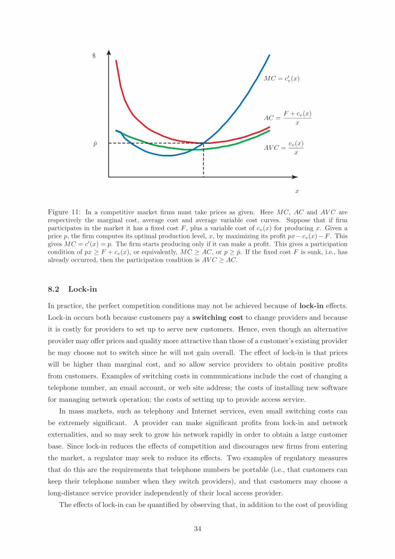
p

x

MC = c′v(x)

AC =F + cv(x)

x

AV C =cv(x)

x

Figure 11: In a competitive market firms must take prices as given. Here MC, AC and AV C arerespectively the marginal cost, average cost and average variable cost curves. Suppose that if firmparticipates in the market it has a fixed cost F , plus a variable cost of cv(x) for producing x. Given aprice p, the firm computes its optimal production level, x, by maximizing its profit px− cv(x)−F . Thisgives MC = c′(x) = p. The firm starts producing only if it can make a profit. This gives a participationcondition of px ≥ F + cv(x), or equivalently, MC ≥ AC, or p ≥ p. If the fixed cost F is sunk, i.e., hasalready occurred, then the participation condition is AV C ≥ AC.

8.2 Lock-in

In practice, the perfect competition conditions may not be achieved because of lock-in effects.

Lock-in occurs both because customers pay a switching cost to change providers and because

it is costly for providers to set up to serve new customers. Hence, even though an alternative

provider may offer prices and quality more attractive than those of a customer’s existing provider

he may choose not to switch since he will not gain overall. The effect of lock-in is that prices

will be higher than marginal cost, and so allow service providers to obtain positive profits

from customers. Examples of switching costs in communications include the cost of changing a

telephone number, an email account, or web site address; the costs of installing new software

for managing network operation; the costs of setting up to provide access service.

In mass markets, such as telephony and Internet services, even small switching costs can

be extremely significant. A provider can make significant profits from lock-in and network

externalities, and so may seek to grow his network rapidly in order to obtain a large customer

base. Since lock-in reduces the effects of competition and discourages new firms from entering

the market, a regulator may seek to reduce its effects. Two examples of regulatory measures

that do this are the requirements that telephone numbers be portable (i.e., that customers can

keep their telephone number when they switch providers), and that customers may choose a

long-distance service provider independently of their local access provider.

The effects of lock-in can be quantified by observing that, in addition to the cost of providing

34

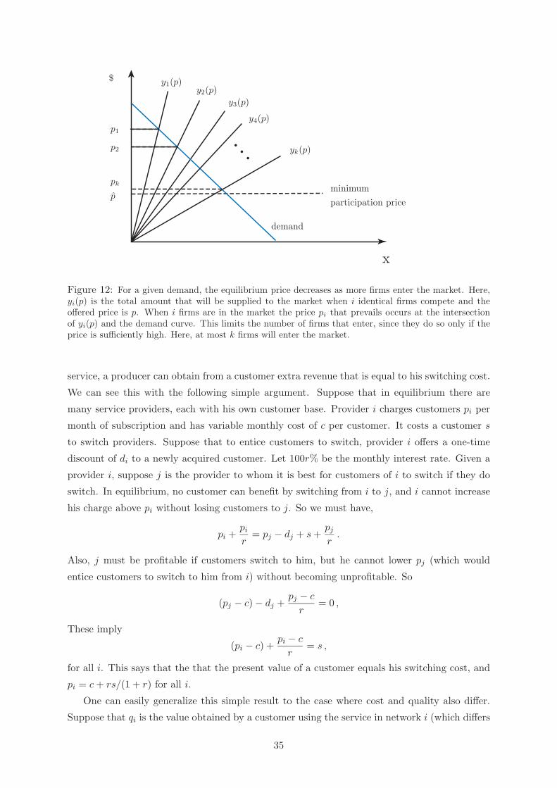
x

$

p

p1

p2

pk

demand

minimumparticipation price

yk(p)

y1(p)y2(p)

y3(p)

y4(p)

Figure 12: For a given demand, the equilibrium price decreases as more firms enter the market. Here,yi(p) is the total amount that will be supplied to the market when i identical firms compete and theoffered price is p. When i firms are in the market the price pi that prevails occurs at the intersectionof yi(p) and the demand curve. This limits the number of firms that enter, since they do so only if theprice is sufficiently high. Here, at most k firms will enter the market.

service, a producer can obtain from a customer extra revenue that is equal to his switching cost.

We can see this with the following simple argument. Suppose that in equilibrium there are

many service providers, each with his own customer base. Provider i charges customers pi per

month of subscription and has variable monthly cost of c per customer. It costs a customer s

to switch providers. Suppose that to entice customers to switch, provider i offers a one-time

discount of di to a newly acquired customer. Let 100r% be the monthly interest rate. Given a

provider i, suppose j is the provider to whom it is best for customers of i to switch if they do

switch. In equilibrium, no customer can benefit by switching from i to j, and i cannot increase

his charge above pi without losing customers to j. So we must have,

pi +pi

r= pj − dj + s +

pj

r.

Also, j must be profitable if customers switch to him, but he cannot lower pj (which would

entice customers to switch to him from i) without becoming unprofitable. So

(pj − c) − dj +pj − c

r= 0 ,

These imply

(pi − c) +pi − c

r= s ,

for all i. This says that the that the present value of a customer equals his switching cost, and

pi = c + rs/(1 + r) for all i.

One can easily generalize this simple result to the case where cost and quality also differ.

Suppose that qi is the value obtained by a customer using the service in network i (which differs

35

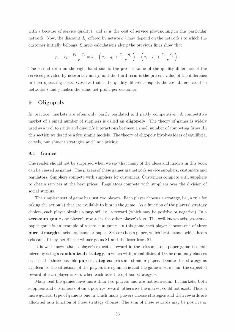
with i because of service quality), and ci is the cost of service provisioning in this particular

network. Now, the discount dij offered by network j may depend on the network i to which the

customer initially belongs. Simple calculations along the previous lines show that

pi − ci +pi − ci

r= s +

(qi − qj +

qi − qj

r

)−

(ci − cj +

ci − cj

r

).

The second term on the right hand side is the present value of the quality difference of the

services provided by networks i and j, and the third term is the present value of the difference

in their operating costs. Observe that if the quality difference equals the cost difference, then

networks i and j makes the same net profit per customer.

9 Oligopoly

In practice, markets are often only partly regulated and partly competitive. A competitive

market of a small number of suppliers is called an oligopoly. The theory of games is widely

used as a tool to study and quantify interactions between a small number of competing firms. In

this section we describe a few simple models. The theory of oligopoly involves ideas of equilibria,

cartels, punishment strategies and limit pricing.

9.1 Games

The reader should not be surprised when we say that many of the ideas and models in this book

can be viewed as games. The players of these games are network service suppliers, customers and

regulators. Suppliers compete with suppliers for customers. Customers compete with suppliers

to obtain services at the best prices. Regulators compete with suppliers over the division of

social surplus.

The simplest sort of game has just two players. Each player chooses a strategy, i.e., a rule for

taking the action(s) that are available to him in the game. As a function of the players’ strategy

choices, each player obtains a pay-off, i.e., a reward (which may be positive or negative). In a

zero-sum game one player’s reward is the other player’s loss. The well-known scissors-stone-

paper game is an example of a zero-sum game. In this game each player chooses one of three

pure strategies: scissors, stone or paper. Scissors beats paper, which beats stone, which beats

scissors. If they bet $1 the winner gains $1 and the loser loses $1.

It is well known that a player’s expected reward in the scissors-stone-paper game is maxi-

mized by using a randomized strategy, in which with probabilities of 1/3 he randomly chooses

each of the three possible pure strategies: scissors, stone or paper. Denote this strategy as

σ. Because the situations of the players are symmetric and the game is zero-sum, the expected

reward of each player is zero when each uses the optimal strategy σ.

Many real life games have more than two players and are not zero-sum. In markets, both

suppliers and customers obtain a positive reward, otherwise the market could not exist. Thus, a

more general type of game is one in which many players choose strategies and then rewards are

allocated as a function of these strategy choices. The sum of these rewards may be positive or

36

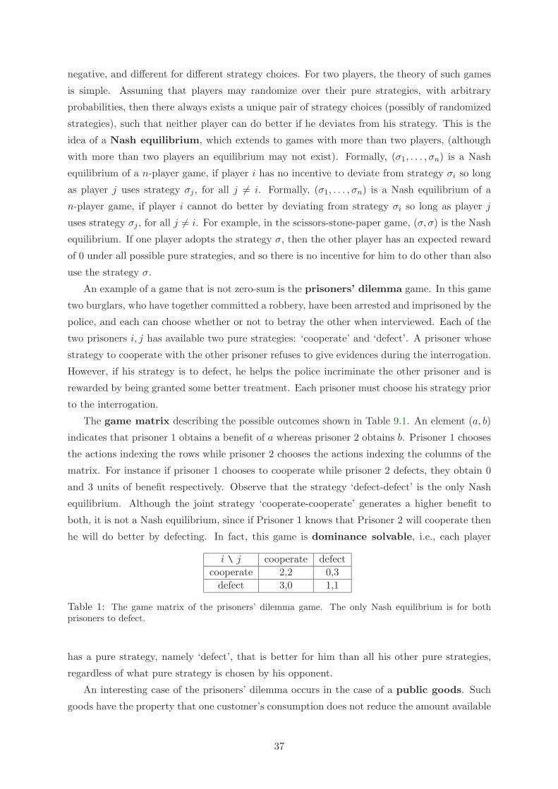
negative, and different for different strategy choices. For two players, the theory of such games

is simple. Assuming that players may randomize over their pure strategies, with arbitrary

probabilities, then there always exists a unique pair of strategy choices (possibly of randomized

strategies), such that neither player can do better if he deviates from his strategy. This is the

idea of a Nash equilibrium, which extends to games with more than two players, (although

with more than two players an equilibrium may not exist). Formally, (σ1, . . . , σn) is a Nash

equilibrium of a n-player game, if player i has no incentive to deviate from strategy σi so long

as player j uses strategy σj , for all j �= i. Formally, (σ1, . . . , σn) is a Nash equilibrium of a

n-player game, if player i cannot do better by deviating from strategy σi so long as player j

uses strategy σj , for all j �= i. For example, in the scissors-stone-paper game, (σ, σ) is the Nash

equilibrium. If one player adopts the strategy σ, then the other player has an expected reward

of 0 under all possible pure strategies, and so there is no incentive for him to do other than also

use the strategy σ.

An example of a game that is not zero-sum is the prisoners’ dilemma game. In this game

two burglars, who have together committed a robbery, have been arrested and imprisoned by the

police, and each can choose whether or not to betray the other when interviewed. Each of the

two prisoners i, j has available two pure strategies: ‘cooperate’ and ‘defect’. A prisoner whose

strategy to cooperate with the other prisoner refuses to give evidences during the interrogation.

However, if his strategy is to defect, he helps the police incriminate the other prisoner and is

rewarded by being granted some better treatment. Each prisoner must choose his strategy prior

to the interrogation.

The game matrix describing the possible outcomes shown in Table 9.1. An element (a, b)

indicates that prisoner 1 obtains a benefit of a whereas prisoner 2 obtains b. Prisoner 1 chooses

the actions indexing the rows while prisoner 2 chooses the actions indexing the columns of the

matrix. For instance if prisoner 1 chooses to cooperate while prisoner 2 defects, they obtain 0

and 3 units of benefit respectively. Observe that the strategy ‘defect-defect’ is the only Nash

equilibrium. Although the joint strategy ‘cooperate-cooperate’ generates a higher benefit to

both, it is not a Nash equilibrium, since if Prisoner 1 knows that Prisoner 2 will cooperate then

he will do better by defecting. In fact, this game is dominance solvable, i.e., each player

i \ j cooperate defectcooperate 2,2 0,3

defect 3,0 1,1

Table 1: The game matrix of the prisoners’ dilemma game. The only Nash equilibrium is for bothprisoners to defect.

has a pure strategy, namely ‘defect’, that is better for him than all his other pure strategies,

regardless of what pure strategy is chosen by his opponent.

An interesting case of the prisoners’ dilemma occurs in the case of a public goods. Such

goods have the property that one customer’s consumption does not reduce the amount available

37

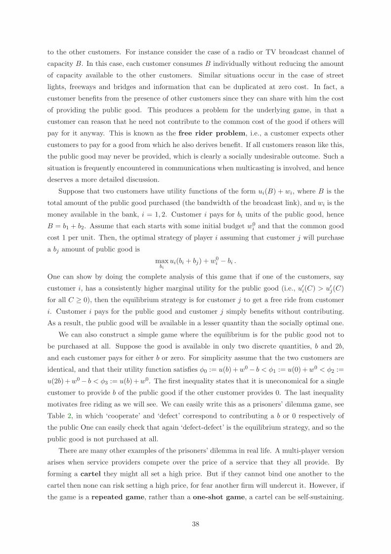
to the other customers. For instance consider the case of a radio or TV broadcast channel of

capacity B. In this case, each customer consumes B individually without reducing the amount

of capacity available to the other customers. Similar situations occur in the case of street

lights, freeways and bridges and information that can be duplicated at zero cost. In fact, a

customer benefits from the presence of other customers since they can share with him the cost

of providing the public good. This produces a problem for the underlying game, in that a

customer can reason that he need not contribute to the common cost of the good if others will

pay for it anyway. This is known as the free rider problem, i.e., a customer expects other

customers to pay for a good from which he also derives benefit. If all customers reason like this,

the public good may never be provided, which is clearly a socially undesirable outcome. Such a

situation is frequently encountered in communications when multicasting is involved, and hence

deserves a more detailed discussion.

Suppose that two customers have utility functions of the form ui(B) + wi, where B is the

total amount of the public good purchased (the bandwidth of the broadcast link), and wi is the

money available in the bank, i = 1, 2. Customer i pays for bi units of the public good, hence

B = b1 + b2. Assume that each starts with some initial budget w0i and that the common good

cost 1 per unit. Then, the optimal strategy of player i assuming that customer j will purchase

a bj amount of public good is

maxbi

ui(bi + bj) + w0i − bi .

One can show by doing the complete analysis of this game that if one of the customers, say

customer i, has a consistently higher marginal utility for the public good (i.e., u′i(C) > u′

j(C)

for all C ≥ 0), then the equilibrium strategy is for customer j to get a free ride from customer

i. Customer i pays for the public good and customer j simply benefits without contributing.

As a result, the public good will be available in a lesser quantity than the socially optimal one.

We can also construct a simple game where the equilibrium is for the public good not to

be purchased at all. Suppose the good is available in only two discrete quantities, b and 2b,

and each customer pays for either b or zero. For simplicity assume that the two customers are

identical, and that their utility function satisfies φ0 := u(b) + w0 − b < φ1 := u(0) + w0 < φ2 :=

u(2b)+w0 − b < φ3 := u(b)+w0. The first inequality states that it is uneconomical for a single

customer to provide b of the public good if the other customer provides 0. The last inequality

motivates free riding as we will see. We can easily write this as a prisoners’ dilemma game, see

Table 2, in which ‘cooperate’ and ‘defect’ correspond to contributing a b or 0 respectively of

the public One can easily check that again ‘defect-defect’ is the equilibrium strategy, and so the

public good is not purchased at all.

There are many other examples of the prisoners’ dilemma in real life. A multi-player version

arises when service providers compete over the price of a service that they all provide. By

forming a cartel they might all set a high price. But if they cannot bind one another to the

cartel then none can risk setting a high price, for fear another firm will undercut it. However, if

the game is a repeated game, rather than a one-shot game, a cartel can be self-sustaining.

38

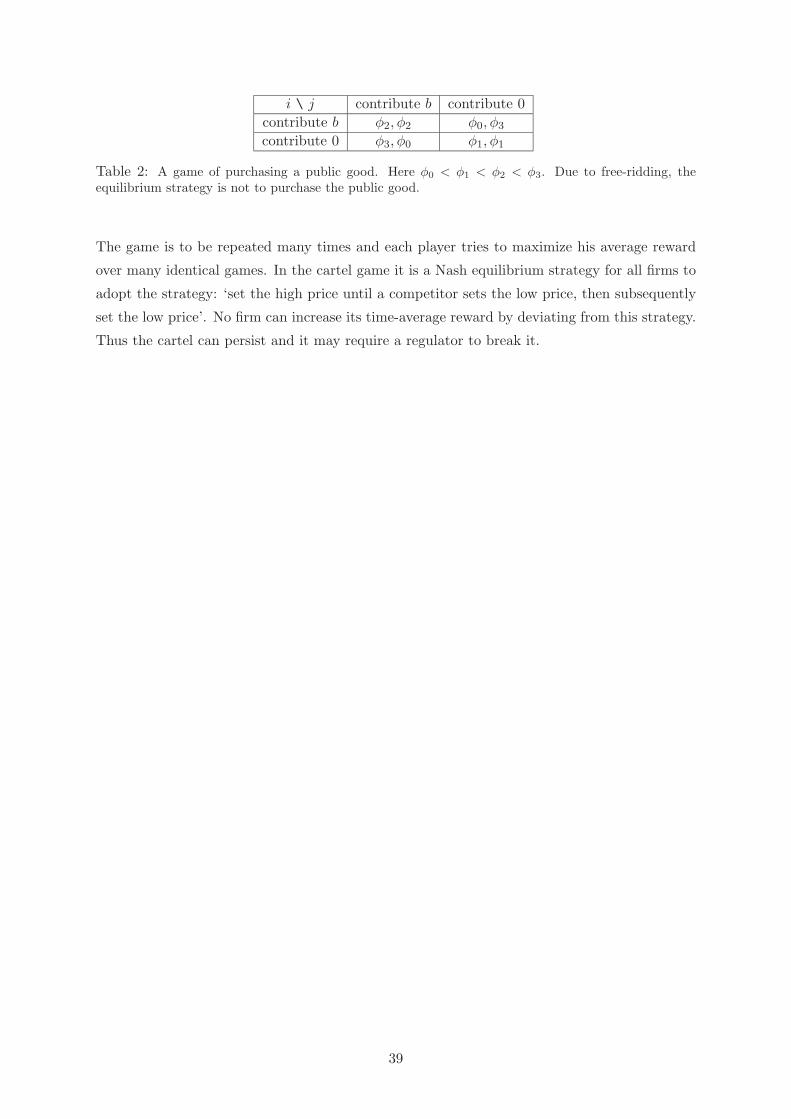
i \ j contribute b contribute 0contribute b φ2, φ2 φ0, φ3

contribute 0 φ3, φ0 φ1, φ1

Table 2: A game of purchasing a public good. Here φ0 < φ1 < φ2 < φ3. Due to free-ridding, theequilibrium strategy is not to purchase the public good.

The game is to be repeated many times and each player tries to maximize his average reward

over many identical games. In the cartel game it is a Nash equilibrium strategy for all firms to

adopt the strategy: ‘set the high price until a competitor sets the low price, then subsequently

set the low price’. No firm can increase its time-average reward by deviating from this strategy.

Thus the cartel can persist and it may require a regulator to break it.

39