This content has been downloaded from IOPscience. Please scroll down to see the full text.

Download details:

IP Address: 128.176.40.239

This content was downloaded on 12/07/2017 at 14:25

Please note that terms and conditions apply.

Basic mathematical and electromagnetic concepts of the biomagnetic inverse problem

View the table of contents for this issue, or go to the journal homepage for more

1987 Phys. Med. Biol. 32 11

(http://iopscience.iop.org/0031-9155/32/1/004)

Home Search Collections Journals About Contact us My IOPscience

You may also be interested in:

Magnetoencephalography - a noninvasive brain imagingmethod with 1 ms time resolution

Cosimo Del Gratta, Vittorio

Pizzella, Franca Tecchio et al.Multipolar modelling in MEG

K Jerbi, J C Mosher, S Baillet et al.

Feasibility of the homogeneous head model in the interpretation of neuromagnetic fields

M S Hamalainen and J Sarvas

The role of model and computational experiments in the biomagnetic inverse problem

B N Cuffin

Magnetoencephalography - the Use of Multi-SQUID Systems for Noninvasive Brain Research

Jukka Knuutila

MEG source models and physiology

Y Okada, M Lauritzen and C Nicholson

A sensor-weighted overlapping-sphere head model and exhaustive head model comparison for MEG

M X Huang, J C Mosher and R M Leahy

The biomagnetic inverse problem: some theoretical and practical considerations

R Harrop, H Weinberg, P Brickett et al.

Phys. Med. Biol., 1987, Vol. 32, No 1, 11-22. Printed in the UK

Basic mathematical and electromagnetic concepts of the biomagnetic inverse problem

Jukka Sarvas Low Temperature Laboratory, Helsinki University of Technology, SF-02150 Espoo, Finland

Abstract. In this paper basic mathematical and physical concepts of the biomagnetic inverse problem are reviewed with some new approaches. The forward problem is discussed for both homogeneous and inhomogeneous media. Geselowitz’ formulae and a surface integral equation are presented to handle a piecewise homogeneous conductor. The special cases of a spherically symmetric conductor and a horizontally layered medium are discussed in detail.

The non-uniqueness of the solution of the magnetic inverse problem is discussed and the difficulty caused by the contribution of the electric potential to the magnetic field outside the conductor is studied. As practical methods of solving the inverse problem, a weighted least-squares search with confidence limits and the method of minimum norm estimate are discussed.

1. Introduction

Biomagnetic fields are caused by electric currents in conducting body tissues like the brain, the heart and the muscles or, by magnetised material, as in lung contamination. The inverse problem is the search for the unknown sources by analysis of the measured field data. To handle this task one must first study the forward problem, i.e. how the magnetic field and the electric potential arise from a known source. For practical purposes, one also has to choose appropriate models for the source and the biological object as a conductor. In this paper basic mathematical and physical concepts of the forward and inverse problems are reviewed and some new approaches are discussed.

In 9 2 of this paper the forward problem is discussed. Only fields due to electric source currents are considered. We describe how the magnetic induction B and the electric potential V are computed using the quasistatic approximation of Maxwell’s equations. The field B is obtained from the total current density J = J ‘ - a V V by the Biot-Savart law. Here J ’ is the impressed source current, - a V V is the Ohmic current and a is the conductivity. The potential V is obtained by solving Poisson’s equation A V = V * J ‘ / a with proper boundary conditions.

In § 3 we show how the above approach easily yields formulae for computing V and B in a homogeneous unbounded medium for a point, line, surface or volume source.

In § 4 the more involved case of an inhomogeneous conductor is discussed. Geselowitz’ formula is introduced which explicitly shows how the magnetic induction is coupled with the electric potential. A surface integral equation for V is derived, which provides means for computing V and B numerically in a general case. However, in the special cases of a spherically symmetric conductor or a horizontally layered conductor, B outside the conductor can be computed in a direct and easy way, and these cases are treated in detail.

In § 5 the inverse problem is discussed. In general, its solution is non-unique, owing to the existence of so-called ‘magnetically silent’ current sources; Some examples

0031-9155/87/010011+ 12$02.50 @ 1987 IOP Publishing Ltd 11

12 J Sarvas

of such sources will be presented. The magnetic inverse problem is also complicated by the coupling between V and B. However, in some special cases this coupling is not present and, accordingly, the inverse problem becomes easier. If, in addition, the potential V is measured on the surface of the conductor, the inverse problem again becomes simpler, and, for instance, for a bounded homogeneous conductor the coupling between V and B can be removed from the problem.

In $0 6 and 7 practical methods of solving the inverse problem are considered. If the unknown source can be described in terms of a limited number of parameters, the solution often becomes unique and an appropriate least-squares search can be applied to determine these parameters. If the measurements involve correlated noise, proper weights must be introduced in the sum of squares which is to be minimised. Statistical confidence limits of the parameters are also discussed. If the measured field depends linearly on the source parameters, the least-squares solution is readily obtained. However, non-uniqueness or numerical instability may be present. Such a linear case can be dealt with by the Moore-Penrose inverse and an appropriate regularisation. A linear inverse problem is also obtained if we seek an estimate for the unknown source as a linear combination of the lead fields. We describe how this estimate is obtained as the minimum norm solution.

Here are some remarks on the notation. The set of real numbers is denoted by R and the n-dimensional Euclidean space by R". For a matrix or a vector, T stands for the transpose. For x = (x,, . . . , X , ) ~ E R" the norm is IlxII = (x:+. . . +x ; )~ '~ . If G is a region or three-dimensional body in R 3 , the surface of G is denoted by dG.

2. Field equations

In this section we consider how the magnetic and electric fields arise from a source current density J ' . This current, also called the impressed current, is due to the electromotive force impressed by biological activity in conducting tissue. Let J' lie in a conductor G which has conductivity a. For magnetic permeability we assume that p =p,, everywhere. To compute the electric field E and the magnetic induction B caused by the bioelectric source J' , the use of the quasistatic approximation of the Maxwell's equations is justified (Plonsey 1969) and this approximation is stated by the equations

E = - V V (1)

V X B = pLgJ V * B = O ( 2 )

J = J ' + U E (3) where V is the electric potential, J is the total current density and c7E is the Ohmic current. Note that V - J = 0 due to equation ( 2 ) and the vector identity V - V x B = 0. Because J is the total current, B is given by the Biot-Savart law:

B ( r ) =- J ( r ' ) x- du'. p0 I r - r' 4.ir G / r - r'I3

(4)

In fact, with some vector calculus we can show that the integral in equation (4) as a function of r is the solution of equation (2) with B( r ) + 0 as / r / + W.

To obtain E and J, we still must find V. For practical purposes we may assume that a is piecewise constant. Write J = J ' - a V V. Because V * J = 0, we obtain V - ( a V V ) = V - J ' , which, in a region with constant a, yields

A V = V * J ' / a . ( 5 )

Basic concepts of the biomagnetic inverse problem 13

The potential V is the unique solution of equation (5) with the requirement that V ( r ) -$ 0 as Irl +CO and with the boundary conditions

V‘= V” uta V’ / a n = u“a V’la n (6)

on an interface between regions of conductivities U’ and a”. In general, computing V from equation ( 5 ) is a rather heavy numerical procedure. However, in a suitable symmetry, the solution of equation (5) becomes much easier. Such cases are the homogeneous unbounded conductor, a horizontally layered conductor and a spherically symmetric conductor.

In biomagnetism we are usually limited to finding the locations of the current sources on a macroscopic length scale. Then it is convenient to replace J’ by an equivalent current density JP which incorporates J ’ and the effects of microscopic changes in conductivity (Tripp 1983). Formally, J P is defined by equation (3) where all quantities must now be considered on the macroscopic scale. In this paper we always denote the source current by J’ but all our results remain valid if J’ is replaced by J P .

3. Fields in an unbounded homogeneous medium

Suppose that the conductor consists of the whole space with constant conductivity U.

Then equation (5) is Poisson’s equation with the solution

V ( r ) = -- l I v; * J ’ ( r ’ )

dv‘ 45-U G r-r‘j ( 7 )

where the integration is over a region G containing the source J ‘ . Using the vector identity V ’ . ( J ’ ( r ’ ) I r - r’1-I) = Ir-r’l-’V’ - J i ( r ’ ) + J i ( r ’ ) - V‘( l r - r’1-I) with V’( l r - r’1-I) = Ir - r ’ ( -3 ( r - r’) and the Gauss theorem we can transform equation ( 7 ) to the form

V ( r ) =- J’( r ’ ) - - dv’ l I

r - r ’ 45-U G ( r - rrI3 (8)

because the surface integral jaGJ’(r’) lr - r’1-I * d S = 0 since J’ = 0 on the boundary aG of G. Equation (8) is a convenient formula for V because it is also valid for J ’ which is not differentiable everywhere.

We can also transform equation (4) for B. Using the identity V ‘ x ( J ( r’)lr - r’l”) = Ir - r’I-’V’ x J ( r ’ ) + V ’ ( ( r - r‘1-I) x J ( r ’ ) and Stokes’ theorem we obtain

B ( r ) =- F,, V ’ x J ( r ’ ) 45- I, / r - r’/

dv’. (9)

Now, J = J ’ - u V V by equation (3), and so V X J = V X J ’ - (TV xVV. Also, since the curl of a gradient vanishes, we have

V ’ x J ’ B ( r ) =e I, j q d v’ (10)

and, carrying out the previous transform backwards, we obtain

B ( r ) =e jG J ’ ( r ‘ ) x- r - r’ Ir - r’I3 du’. (11)

We see that in the homogeneous space the total current in equation (4) can be replaced by the impressed current J ’ . In other words the volume current UE does not contribute to B in this case.

14 J Sarvas

Next we consider V and B due to a dipolar point source. A current dipole with a moment Q is a concentration of the impressed current to a single point ro: J ’ ( r ) = 6( r - ro) Q, where 6 ( r ) is the Dirac delta function. Equations (8) and (1 1) readily yield V and B for a dipole in the homogeneous space:

1 r - ro 4rra Ir - rOl3

V ( r ) = - Q-- (12)

PO r - ro B ( r ) =- Q x -

4rr Ir - rol3‘ (13)

A current dipole is a good approximation for a small source viewed from a remote field point: if J ‘ is confined to a small region G with ro in G and r is far from ro , then equation (11) yields

B ( r ) = - J ’ ( r ‘ ) x - d v ’ - - r - r ’ r - ro

P0 Q x - Ir - r’I3 4rr Ir- rol3 Po I 4rr G

(14)

where Q = jG J ’ ( r ’ ) dv‘. So, B due to J’ can be approximated by the field of the current dipole Q at r, . A similar result is valid for V. It can also be shown that a small source in a bounded and inhomogeneous conductor can be approximated by a dipole.

If the source current is distributed on a line or a curve or on a surface, equations (8) and (1 1) remain valid if we replace the volume density J ’ by a line or a surface density and the volume integral by a line or a surface integral, respectively.

4. Fields in an inhomogeneous medium

Let G be a bounded conductor with a piecewise constant conductivity U and with U = 0 outside G. Further, let G be divided by surfaces S,, j = 1,. . . , n, into subregions Gj, j = 1, . , . , n, so that U = uj in each G,. We will derive useful representations for B and V in terms of J ‘ and the values of V on Si, j = 1,. . . , n, caused by J ‘ in G,.

First we consider the magnetic field. From equations (3) and ( l l ) ,

B( r ) = - [ J ’ ( r ’ ) - U( r’)V V ( r ‘ ) ] X - r - r ’ r; I,; Ir - r’I3 dv’

= B o ( r ) - - c U, V V ( r ’ ) x - dv‘ (15) Po Il r - r ’ 4rr ,=, Ir - rtI3 I,;

where

Bo( r ) = - J‘( r ‘ ) x - d v’ Po I r - r’ 477 G Ir - r’I3

(16)

is the magnetic induction due to J ‘ in a homogeneous space. Using the identity V X ( V V g ) = V V X V g with V g = Ir - r’Ip3(r - r ’ ) and Stokes’ theorem, we obtain

L V V ( r ’ ) x - d o ’ = V ( r ’ ) n ( r ’ ) x - dS, Ir - r’I3

r - r ’ r - r ’ Ir - rrI3 IaGl

where n is the outer unit normal of the surface aG,. This result, with equation (15), implies Geselowitz’ formula (Geselowitz 1970)

B ( r ) = B o ( r ) - - 2 (U;-U;’) V ( r ’ ) n ( r ‘ ) x - dS, (17) Po t7 r - r ’ 4rr j = , ( r - r’I3 I,;

Basic concepts of the biomagnetic inverse problem 15

for all r not on any surface S,. Here U,! and U:’ are the conductivities on the inner and outer sides of S,, respectively. This result shows how the volume currents -uV V affect B. Their contribution is equal to the field arising from surface current distributions -(U: - U,!’) V ( r ’ ) n ( r ’ ) , r ’ E S, , j = 1, . . . , n, in a homogeneous space. These fictitious sources on the surfaces are often called secondary currents.

Using Green’s identity and boundary conditions from equation (6) it is not difficult to obtain a representation similar to equation (17) for V (Geselowitz 1967):

a ( r ) V ( r ) = u , V , ( r ) - C -1 v ( r ’ ) n ( r ’ ) * - n u ! -u ! t r - r ’

d SJ (18) , = I 4~ S , Ir - rtI3

with r in G but not on any of the surfaces S,. Here V, is the potential given by (8) with U = un.

Equation (18) can be used to derive a surface integral equation for V, which then can be employed as the starting point for the numerical calculation of V. With this in mind, let r approach a point S on S, from inside. It is known that the integral over S, in equation (18) is not continuous in r as r tends to S. However, we have the following result (Vladimirov 1971): if the integral over S, is denoted by F j ( r ) , then

lim F J ( r ) = - 2 ~ V ( s ) + F,(s) I-S

with r inside the surface S,. This result, with equation (18), yields the integral equation for V : for each r on S, , k = 1, . . . , n, we have

ai, + U: V ( r ) = o , V , ( r ) - 1 a V ( r ’ ) n ( r ’ ) . - dS,. (19)

n U!“ ! ‘ r - r ‘ 2 / = l 4.rr Is, / r - r’I3

Equations (17) and (19) provide the means for computing V and B for given G and J’ . First, we numerically solve equation (19) for V (Barnard et a1 1967). Next, we obtain V in G from equation (18) and B from equation (17). This method works well for bounded homogeneous conductors. It is also applicable in bounded inhomogeneous conductors provided that the conductivity steps on the surfaces Si are not too high. The method has been used in cardiac studies with the body modelled to consist of homogeneous parts: the lungs and the rest of the body (Barnard er a1 1967, Cuffin and Geselowitz 1977). It has also been applied in neuromagnetism with the head modelled as a homogeneous conductor (Hamalainen and Sarvas 1987).

Next we consider two special cases where B is much easier to compute: a spherically symmetric conductor and a horizontally layered conductor. Suppose now that G is bounded and spherically symmetric with respect to some origin. Surfaces S, are then concentric spheres. First we show that for any J’ in G the radial compoment E , of B coincides with that of Bo in equation (16) outside G. From equation (17) we have

E r ( r ) = B o ( r ) - e r - - C (uj-uj ‘ ) V ( r ’ ) n ( r ‘ ) x - - e r d v t . F0 Il r - r ’ 4 T j - l l,, Ir - r‘I3

(20)

In the above integrals the scalar triple product vanishes because n( r ’ ) = r’/ lr’) and e, = r/lrl . Therefore the integrals in equation (20) vanish, and for all r outside G

E r ( r ) = E o r ( r ) = - J ’ x - - e r d v ‘ . :i I, Ir - 43 r - r ‘

(21)

Although the other components of B receive a contribution from the volume currents

16 J Sarvas

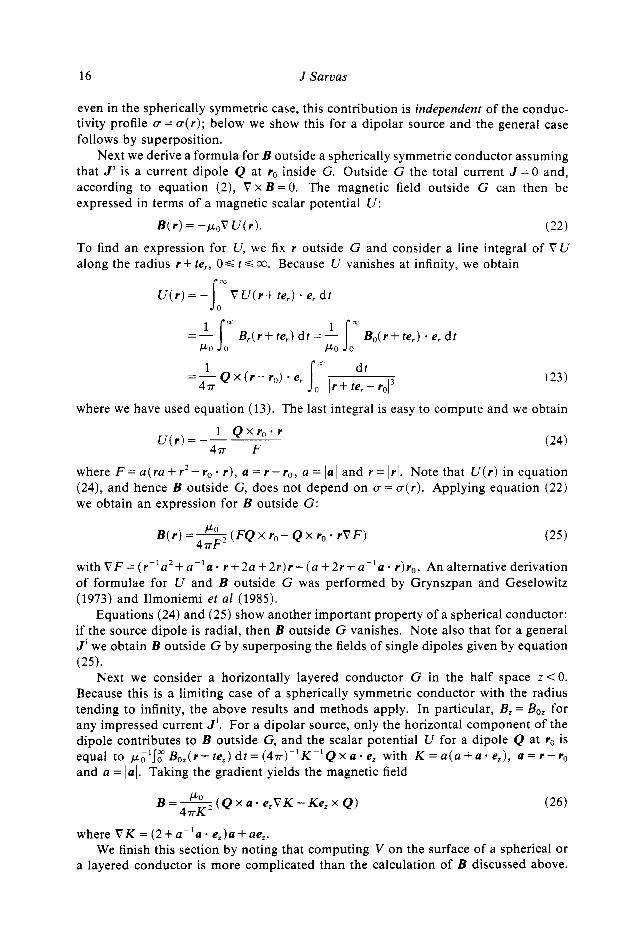
even in the spherically symmetric case, this contribution is independent of the conduc- tivity profile U = u( r ) ; below we show this for a dipolar source and the general case follows by superposition.

Next we derive a formula for B outside a spherically symmetric conductor assuming that J' is a current dipole Q at ro inside G. Outside G the total current J = O and, according to equation (2), V x B = O . The magnetic field outside G can then be expressed in terms of a magnetic scalar potential U :

B ( r ) = - p o V U ( r ) . (22)

To find an expression for U, we fix r outside G and consider a line integral of V U along the radius r + re,, 0 s t s CO. Because U vanishes at infinity, we obtain

U ( r ) = -loE V U ( r + te,) * e, dt

X =Ll B , ( r + t e , ) d t = - B , ( r + t e , ) . e , d t Po 0 Po 1 lX 0

1 lo x dt = - Q x ( r - r o ) ~ e , 47r 1 r + re, - pol3

(23)

where we have used equation (13). The last integral is easy to compute and we obtain

U ( r ) = -- l Q x r o . r 47r F (24)

where F = a( ra + r2 - ro * r ) , a = r - rO, a = 141 and r = Irl. Note that U ( r ) in equation (24), and hence B outside G, does not depend on u = u ( r ) . Applying equation (22) we obtain an expression for B outside G:

B ( r ) = - ( F Q x r , - Q x r , . r V F ) PO 47rF2 (25)

w i t h V F = ( r " a 2 + a " a . r + 2 a + 2 r ) r - ( a + 2 r + a " a . r ) r o . Analternativederivation of formulae for U and B outside G was performed by Grynszpan and Geselowitz (1973) and Ilmoniemi et al (1985).

Equations (24) and (25) show another important property of a spherical conductor: if the source dipole is radial, then B outside G vanishes. Note also that for a general J' we obtain B outside G by superposing the fields of single dipoles given by equation

Next we consider a horizontally layered conductor G in the half space z < 0. Because this is a limiting case of a spherically symmetric conductor with the radius tending to infinity, the above results and methods apply. In particular, B, = Bo, for any impressed current J ' . For a dipolar source, only the horizontal component of the dipole contributes to l? outside G, and the scalar potential U for a dipole Q at ro is equal to ~ C L g ~ ~ ~ B ~ ~ ( r + t e , ) d t = ( 4 7 r ) " K " Q x a ~ e , with K = a ( a + a . e , ) , a = r - r o and a = 1 0 ) . Taking the gradient yields the magnetic field

(25).

B = - P O ( Q x a . e , V K - K e , x Q ) (26) 4 r K 2

where V K = ( 2 + a " a . e z ) a + a e z . We finish this section by noting that computing V on the surface of a spherical or

a layered conductor is more complicated than the calculation of B discussed above.

Basic concepts of the biomagnetic inverse problem 17

Furthermore, radial sources usually produce a non-constant V on the surface of such a conductor.

5. The inverse problem

The magnetic inverse problem is to find J’ from measurements of B outside G. As is well known, the problem has no unique solution. This is due to the fact that there are so-called magnetically silent sources, which produce no B outside G. Such a current source can always be added to a solution of the inverse problem without affecting the field outside G.

An example of a magnetically silent source is a radial current dipole in a spherically symmetric conductor. From equation (17) it is not difficult to see that an axially symmetric impressed current in a cylindrical conductor is silent as well. If S is a closed surface in G and J ’ is a uniform surface current normal to S, then J ’ is silent. To see this, use equation (17) , Stokes’ theorem and note that V = 0 because V, in equation (18) vanishes due to equation (8) and Gauss’ theorem. If G is a bounded homogeneous conductor, an impressed current of the form J’ = V q , with J’ * n = 0 on the boundary of G, is magnetically silent. Namely, V = cp/u is the potential for this source because it satisfies Poisson’s equation ( 5 ) and the boundary conditions (6). It follows that J = 0 and, consequently, B = 0.

The magnetic inverse problem is also complicated by the fact that V affects B according to equation (17). However, if V * J ‘ = 0, then V = 0 and B is given by equation (16). In particular, this is the case if J’ is a closed current loop. For such a loop the inverse problem has a unique solution.

If G is spherically symmetric, then B, does not depend on V and the magnetic inverse problem becomes easier. For instance, consider a vertical rectangular plate P in a spherically symmetric conductor and a perpendicular current dipole distribution on P. It is not difficult to show that this source is uniquely determined by B outside G. Applied to neuromagnetism, this model could describe the sources on the wall of a fissure when the head is modelled as a spherical conductor.

If, in addition to B, we also measure V on the surface of the conductor, the inverse problem is made easier-at least in principle. For example, consider a bounded homogeneous conductor. Then equation (17) yields

B , ( r ) = B ( r ) + - V ( r ’ ) n ( r ’ ) x - r - r ’

Ir - r‘l3 d S (27) POU

4 n I,,

for all r outside G. So, if we know V on aG and B outside G, we obtain B,, outside G, and can try to find J’ from equation (16), which does not involve V any more. On the other hand, the knowledge of V on aG can be utilised to get additional knowledge about J’ . With Green’s identity we can show that

1 - V(r’)- - d S =- J’(r ’ ) . - dv’ = V,( r ) . (28) r - r ’ ‘ 1 477 I,, lr - rq3

r - r ‘ ( r - r’I3 477g G

If V is known on aG, the above result yields V, outside G, and from equation (28) we possibly get additional information concerning J‘ . However, even equations (16)

18 J Sarvas

and (28) together usually do not determine J' uniquely. To make the solution unique we must add some extra information to restrict the possible source configurations. For a general review of the inverse problems see, for instance, Sabatier (1977, 1983) and Parker (1977).

6. Non-linear inverse problem and the least-squares search

If in the inverse problem the unknown source can be described in terms of a limited number of unknown parameters P I , . . . , pm E R and the solution is unique, an appropri- ate least-squares search is a practical way of solving the respective inverse problem. The method requires, however, that we can solve the corresponding forward problem in the given conductor geometry.

Let us consider a typical situation. Suppose that f i i is the measured component of B at point Pi of the measurement grid, i = 1, . . . , n, and let B,@) be the corresponding computed field value at P, for given parameters p = (p1,. . . , R".

We assume that B ( P ) = ( B , ( P ) , . . . , is a non-linear function of p ; the linear case is treated in the next section. A typical non-linear example is an inverse problem where the unknown source is a tangential current dipole in a spherical conductor and where B, is measured outside the conductor (see, e.g., Okada et a1 1984, Ricci et a1 1985, Sams et a1 1985). In this case the source is determined by five parameters ( p , , . . . , p. I

We also assume that every B, contains some noise so that B, = b, + v i , i = 1, . . . , n, where b, is the correct field value and v i is a normally distributed error with zero mean. The errors 7, are possibly correlated with a covariance matrix Q = E[7vT] where v = ( vl, . . . , E is the operator of taking the mean value.

Suppose first that vl,. . . , 7, are independent random variables with zero mean and unit standard deviation, i.e. each 7, is N ( 0 , 1)-distributed or, in other words, Q = I , the identity matrix. We want to find>he source p* which best explains the measurements in the sense that p = (p1, , . , , Pm)T minimises the sum of squares

-

A A

i = l

Because the errors in f i , are independent and have the same noise level, no weight factors are needed in S ( p ) .

If Q # 1, we must replace equation (29) by a new weighted sum. Decompose Q so that Q = VA2 VT where V is an orthogonal matrix, A = diag(A, , . . . , A,) is a diagonal matrix with each A , > 0 and A' = AA. The new sum of squares is given by

where " F ( @ ) = ( F , ( P ) , . . . , Fn(p))T= P B ( p ) , y = ( y l , . . . , Y , , ) ~ = PE, P = VA"VT and B = (B, , . . , , f i n ) T . We may consider y = c + E as new data with the noiseless field values c = (c , , . . . , c , ) ~ = P ( b l , . . . , b,)T and with new noise E = ( E ~ , . . . , E , ) ~ = P ( v , , . . . , v,)T. The new errors E ~ , . . . , E, are independent and N ( 0 , 1)-distributed, because the covariance matrix of E is the identity matrix: = E ( P ~ T ~ P ) = PE( vvT)P = PQP = I. Therefore, the situation is reduced back to equation (29) for F ( P ) and y , and this justifies the choice of equation (30).

Basic concepts of the biomagnetic inverse problem 19

So, we must find p^ E R"' which minimises the sum of squares (30). As assumed, F ( p ) is a non-linear function of p, and we must apply some numTrica1 minimising algorithm, for example, Marquardt's method (Nash 1979), to find p.

After finding the solution p* we need to know how reliable it is, i.e. what is the resolution of our inverse method. This information is given by a confidence region for y, or confidence limits for y,,Awhere y = ( yl , . . . , ym)T is the correct parameter vector which is only estimated by p. Next it is shown how the confidence region and confidence limits are found by linearisation.

Assume that p^ is close to y so that the linear approximatjon can be appliep: F ( p ) = F ( y ) + A ( p - y ) where A is the Jacobian matrix of F at p : A , = ( a F , / a p , ) ( p ) , i = l , . . . , n ; j = 1 , . . . , m. We assume that ATA is a non-singular matrix. Inserting this linear approximation into equation (30) yields a quadratic minimising problem with the well known solution (Golub and Van Loan 1983)

p*= r + ( ~ T ~ ) - ' ~ T ( y - ~ ( y ) ) . (31)

Here y - F ( y ) = y - c = E . We see tha; p* is nymally distributed with mean y and co- variance matrix (ATA)" because E ( ( @ - ? ) ( p - y ) = ) = ( A T A ) " A T E ( ~ ~ T ) A ( A T A ) " = (ATA)" since = I. Therefore, for a solution p*, the confidence ellipsoid for y (Silvey 1978) is G , = { p : ( p - p ) A A(P - p * ) r 2 } . Here r2 is the p-percentage point of the xi distribution: P { x i r2 } = p % . This means that y is in G, with probability p % . Let ATA = A?v,vT be the spectral decomposition of ATA with eigenvalues A f and eigenvectors U, E R". Then

" T T

and we see that G, is an ellipsoid in R"' with the centre p* and the half-axes rA L' U , ,

i = l , . . . , m. Next we consider the p% copidence limip for a parameter yi, i = 1, . . . , m. These

limits are simply the intervals pi - 6, yi p, +Si, where c S i > 0 is the maximal value of - y,I attained in G,. The numbers 6, are easily found by observing that they are just half of the edges of the rectangular box containing GP and having its faces parallel to the coordinate plates, and we obtain 6, = ( u , / A ~ ) ~ ] ~ " , where v, = ( u i l , . . . , These confidence limits are used, for instance, in Kaukoranta et al (1986).

7. Linear inverse problem

We first consider the same inverse problem as in the previous section, but now the function F ( P ) in equation (30) is linear in p and we denote F by the matrix A. To find p^ we have to minimise the quadratic expression S ( p ) = llAP -y1I2, p E R"', y E R".

For example, we obtain a linear inverse problem, if the source is described by a few leading terms of its multipole expansion with a fixed origin (see e.g. Karp er a1 1980), or the source consists of a limited number of current dipoles with fixed locations.

First assume that ATA is non-singular. Then the least-squares solution, which minimises S ( p ) , is given by

p* = ( A ~ A ) - ' A ~ ~ (33)

with the same confidence region, equation (32), and confidence limits as in the non-linear case.

20 J Sarvas

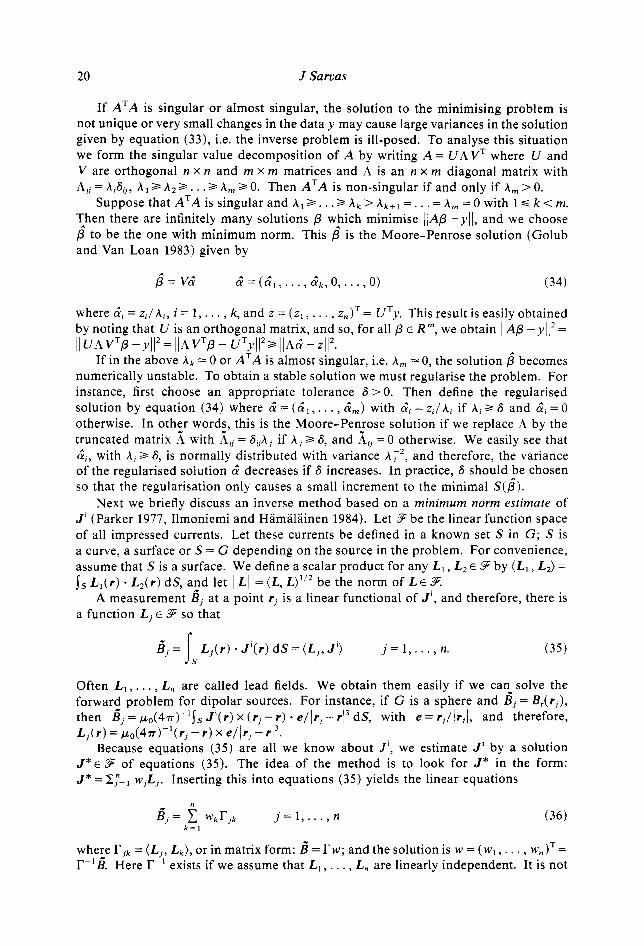
If ATA is singular or almost singular, the solution to the minimising problem is not unique or very small changes in the data y may cause large variances in the solution given by equation (33), i.e. the inverse problem is ill-posed. To analyse this situation we form the singular value decomposition of A by writing A = UA VT where U and V are orthogonal n X n and m X m matrices and A is an n X m diagonal matrix with AV = Ais i j , A , 3 h2 3. . .3 A, 3 0. Then ATA is non-singular if and only if A , > 0.

Suppose that A ~ A is singular and A , 3 . . .a hk > & + l = . . . = A , = o with 1 S k < m. Then there are infinitely many solutions P which minimise IIAP -yll , and we choose p* to be the one with minimum norm. This p* is the Moore-Penrose solution (Golub and Van Loan 1983) given by

p*= Val A A =(a,,. . . , a * k , 0, . . . , 0) (34)

where 6, = z , /A i , i = 1, . . . , k, and z = ( z I , . . . , z , ) ~ = UTy. This result is easily obtained by noting that U is an orthogonal matrix, and so, for all P E R", we obtain llAP -yj12 =

If in the above hk =z 0 or ATA is almost singular, i.e. h, = 0, the solution p* becomes numerically unstable. To obtain a stable solution we must regularise the problem. For instance, first choose an appropriate tolerance S > 0. Then define the regularised solution by equation (34) where & = ( L , , . . . , &,) with a l i = z i / h i if A i 3 S and 6 , = 0 otherwise. In other words, this is the Moore-Penrose solution if we replace A by the truncated matrix A with A,j = S,hj if hi 3 S, and A, = 0 otherwise. We easily see that (Y,, with hi 3 S, is normally distributed with variance A T 2 , and therefore, the variance of the regularised solution 6 decreases if S increases. In practice, S should be chosen so that the regularisation only causes a small increment to the minimal S(p^) .

Next we briefly discuss an inverse method based on a minimum norm estimate of J' (Parker 1977, Ilmoniemi and Hamalainen 1984). Let 9 be the linear function space of all impressed currents. Let these currents be defined in a known set S in G; S is a curve, a surface or S = G depending on the source in the problem. For convenience, assume that S is a surface. We define a scalar product for any L , , L2 E 9 by ( L , , L2) = s s L , ( r ) L 2 ( r ) dS, and let IlLll = ( L , L),'* be the norm of L E 9.

A measurement g j at a point r j is a linear functional of J ' , and therefore, there is a function L j E 9 so that

IIUAVTp-yl12=llAVTP-UTyy)(2~IIAal-~I12.

g j = / s L j ( r ) . J ' ( r ) d S = ( L J , J ' ) j = l , . . . , n. (35)

Often L , , . . . , L, are called lead fields. We obtain them easily if we can- solve the forward problem for dipolar sources. For instance, if G is a sphere and B j = BAr,), then g j = p 0 ( 4 ~ ) " j s J ' ( r ) X ( r , - r ) e / \ r J - , l 3 dS, with e = rj / \r j l , and therefore, L j ( r ) = p0(457-'(r j - r ) X e / l r j - r13.

Because equations (35) are all we know about J ' , we estimate J i by a solution J* E 9 of equations (35). The idea of the method is to look for J* in the form: J* = E;=, wjLj . Inserting this into equations (35) yields the linear equations

where r j k = ( L ~ , L k ) , or in matrix form: E = rW; and the solution is W = (W,, . . . , w,lT= r-lg. Here r-' exists if we assume that L , , . . . , L, are linearly independent. It is not

Basic concepts of the biomagnetic inverse problem 21

difficult to show that J* is the orthogonal projection of J‘ to the subspace of .?F spanned by L , , . . . , L, and, therefore, J* has the minimum norm among all solutions J’ E 9 of equations (35).

For J* to be a reasonable estimate of J’ , it is necessary that the inverse problem has a unique solution, i.e. B outside G uniquely determines J’ . Even in this situation the limited number of measurements and noise may greatly disturb J*.

Furthermore, the solution W = r-lg may be numerically unstable and it needs regularisation. The regularisation method proposed above works here as well. However, we add to it a statistical criterion (Parker 1977), which tells us how much regularising is sufficient.

Let Q = VA2 V’ be the covariance matrix of the errors in g j as in 0 6 . We multiply the equation g = I‘w by P = VA” V’ and obtain an equivalent equation: y = MW with y = P 6 and M = P T . Again, the covariance matrix of y is the identity matrix. Decom- pose M so that M = UDUT where D=diag(A,, . . . , A n ) , A , Z . . . Z A n > O and U is orthogonal. We write the solution W in the form W = Ua with a = D” U’y = (a1,. . . , a,)’. The regularised solution W * is defined by W * = Ua* with a? = a j , j = 1, . . . , k, and af = 0 for j = k + 1, . . . , n. Now we must decide how k < n is chosen; the smaller k is, the more regularisation we get. Because W * no longer solves the equation y = MW* exactly, we may consider the difference y -y* = M ( W - W * ) due to random errors in yi, i = 1, . . . , n. Therefore, the misfit Sk = (yi -yT)) ’ = Ily -y*ll* can be thought to be distributed like ,&k, because there are k ‘model parameters’ a t , . . . , a;. We obtain the required criterion by choosing k so that S, = ro ,5 , where P { ~ ~ - k ~ r ~ . ~ } = O . 5 . Note that s k = I I M ( W - W * ) 1 1 2 = ~ ~ D ( a - n * ) ~ ~ 2 = ~ ~ = k + l Z; with Z =

( z l , . . . , z,)T= u’y.

Acknowledgments

I am grateful to Olli V Lounasmaa and Matti S Hamalainen who read the manuscript and made several constructive remarks. Thanks are also due to Antti Ahonen, Riitta Hari and Elina Kaukoranta for many helpful discussions on the material presented here. This work was supported by the Academy of Finland.

Resume

Concepts mathimatiques et ilectromagnitiques de base du probltme biomagnitique inverse.

Les auteurs prisentent dans ce travail une revue et une nouvelle approche des concepts mathimatiques et physiques de base du p r o b l h e biomagnetique inverse. 11s discutent le problkme direct a propos des milieux homogenes et htterogenes. 11s prisentent la formule de Geselowitz et une equation de I’intigrale de surface pour traiter le cas d’un conducteur homogene ilimentaire. 11s discutent igalement en detail les cas particuliers d’un conducteur B symitrie sphirique et d’un milieu en couches horizontales. La non uniciti de la solution du probleme magnitique inverse fait I’objet d’une discussion, et les auteurs itudient les difficultis entraintes par la contribution du potentiel electrique au champ magnitique en dehors du conducteur. Les auteurs discutent egalement des methodes utilisies en pratique pour risoudre le probleme inverse, c’est-a-dire une mithode de recherche par les moindres carris pondiris, avec limites de confiance, et la mithode de I’estimation de norme minimale.

Zusammenfassung

Grundlegende mathematische und elektromagnetische Konzepte des biomagnetischen inversen Problems.

In dieser Arbeit wird ein Uberblick gegeben iiber die grundlegenden mathematischen und physikalischen Konzepte des biomagnetischen inversen Problems und gleichzeitig auf einige neue Verfahren hingewiesen.

22 J Sarvas

Das 'Forward'-Problem wird sowohl fur homogene wie auch fur inhomogene Medien diskutiert. Die Formeln von Geselowitz und eine Oberflachen-Integralgleichung werden vorgestellt, um eine stiickweise homogene Leitung theoretisch zu behandeln. Die Spezielfalle einer kugelsymmetrischen Leitung und eines horizontal geschichteten Mediums werden ausfiihrlich diskutiert. Die Nicht-Eindeutigkeit der Losung des magnetischen inversen Problems wird diskutiert und die Schwierigkeit durch den Beitrag des elektrischen Potentials zum Magnetfeld auaerhalb der Leitung wird untersucht. AIS praktische Methode zur Losung des inversen Problems werden eine gewichtete Fehlerquadratmethode mit Konfidenzintervallen und die Methode des minimalen Normschatzwertes diskutiert.

References

Barnard A C, Duck I M, Lynn M S and Timlake W P 1967 Biophys. J. 7 463-91 Cuffin B N and Geselowitz D B 1977 IEEE Trans. Biomed. Eng. BME-24 242-52 Geselowitz D B 1967 Biophys. J. 7 1-11 -1970 IEEE Trans. Magn. MAG-6 346-7 Golub G H and Van Loan C F 1983 Matrix Computations (Oxford: North Oxford Academic) p 139 Grynszpan F and Geselowitz D B 1973 Biophys. J. 13 911-25 Hamalainen M S and Sarvas J 1987 Phys. Med. Biol. 32 91-7 Ilmoniemi R J and Hamalainen M S 1984 Helsinki Unioersiiy of Technology Report TKK-F-A559 llmoniemi R J , Hamalainen M S and Knuutila J 1985 Biomagnetism: Applications and Theory ed H Weinberg,

Karp P J, Katila T E, Saarinen M, Siltanen P and Varpula T T 1980 Circulation Res. 47 117-30 Kaukoranta E, Hamalainen M S, Sarvas J and Hari R 1986 Exp. Brain Res. 63 60-6 Nash J C 1979 Compact Numerical Methods for Computers (Bristol: Adam Hilger) Okada Y C, Tanenbaum R, Williamson S J and Kaufrnan L 1984 Exp. Brain Res. 56 197-205 Parker R L 1977 Ann. Rev. Earth Planer. Sci. 5 35-64 Plonsey R 1969 Biornagnetic Phenomena (New York: McGraw-Hill) p 203 Ricci G B, Leoni R, Romani G L, Campitelli F, Buonomo S and Modena I 1985 Biomagnetism: Applicaiions

Sabatier P C 1977 J. Geophys. 43 115-37 -1983 Radio Sci. 18 1-18 Sams M, Hamalainen M, Antervo A, Kaukoranta E, Reinikainen K and Hari R 1985 Eleciroencephalogr.

Silvey S 0 1978 Statistical Inference [London: Chapman and Hall) p 91 Tripp J H 1983 Biomagnerism: an Interdisciplinary Approach ed S J Williamson, G L Romani, L Kaufman

Vladimirov V S 1971 Equations ofkfathematical Physics (New York: Marcel Dekker) p 302

G Stroink and T Katila (Oxford: Pergamon) pp 278-82

and Theory ed H Weinberg, G Stroink and T Katila (Oxford: Pergamon) pp 304-10

Clin. Neurophpsiol. 61 254-6

and I Modena (New York: Plenum) p 123