BASIC PHYSICS OF HIGH

BRIGHTNESS ELECTRON BEAMS

Wai-Keung Lau Winter School on Free Electron Lasers 2017

Jan. 19th 2017

Outline

Basic concepts

Linear Beam optics

Beam emittance

Beam optics with space charge effect

Vlasov model of beams

Beam injectors for free electron lasers

Basic Concepts

Single Particle Dynamics in EM Fields

Relativistic dynamics

Applied EM fields are usually expressed as expanded series called paraxial

approximation

Complicated EM field distributions can only be solved by numerical methods.

Examples of simulation codes are: POISSON/SUPERFISH

High Frequency Structure Simulator (HFSS) -- http://www.ansoft.com/products/hf/hfss/

CST Microwave Studio -- http://www.cst.com/Content/Products/MWS/Overview.aspx

BvEqvmdt

d

dt

pd

0

The Lorentz factor is in general not a constant of time

Lorentz force law

5

Paraxial Approximation of Axisymmetric

Electric and Magnetic Fields General assumptions:

Consider only static electric and magnetic fields at this point.

That is, no time-varying fields and displacement currents are excluded.

Electric and magnetic fields for axisymmetric lenses in a beam focusing system do not usually have azimuthal components (i.e. ).

Other field components have no azimuthal dependence

In paraxial approx., fields are calculated at small radii from the system axis with the assumption that the field vectors make small angles with the axis

0

0

B

E

0

rz EE

zr EE zr BB

0

0

E

B

0

rz BB

0;0 BE

6

Define electrostatic and magnetic potentials such that:

For symmetric fields that satisfies the above assumptions, then

and therefore e and m are functions of r and z only. Therefore, e and m obeys Laplace equation:

The following form for electrostatic potential is useful to derive paraxial approximations for electric fields:

eE

mB

0

rz EE

0

ee

zz

0

ee

rr

01

,2

22

z

f

r

fr

rrzrf

4

4

2

20

2

0

2, rfrffrzfzrf

000

r

rr

rE

xExE

f represents either e or m.

They are not a function of

7

Substitute f into the Laplace equation of function f gives

From recursion formula for the coefficients f2

we have,

Therefore,

or

01222 2

0

2

22

2

1

rfrf

022 222

2 ff

4

0

4

4

02

64

1

4

1

z

ff

ff

4

4

42

2

2 ,0

64

1,0

4

1,0, r

z

zfr

z

zfzfzrf

2

02

2

2

,0

!

1,

r

z

zfzrf

8

Hence, the axial and radial fields

in paraxial approximation are:

4

44

2

22

3

33

644,

162,

z

Er

z

ErEzrE

z

Er

z

ErzrE

z

r

4

44

2

22

3

33

644,

162,

z

Br

z

BrBzrB

z

Br

z

BrzrB

z

r

(1)

(2)

(3)

(4)

the total Coulomb force acting on q by a thin volume dV

of charge Q is independent of r !!

Planar Diode with Space Charge – Child-Langmuir Law

0

2

22

dx

d

constxJ x

02

2 xexm

2/12/1

0

2

2 1

/2

me

J

dx

d

C

me

J

dx

d

2/1

2/1

0

2

/2

4

xm

eJ4/12/1

0

4/3 22

3

4

3/4

0

d

xVx 2

2/3

0

2/1

0

2

9

4

d

V

m

eJ

2

2

2/3

06 /1033.2 mAd

VJ

x

e-

=0

=V0

cathode

C=0 under the boundary conditions: =0 and

d/dx=0 at x=0; the condition d/dx=~x1/3=0 at

x=0 implies that the special case electric field

at cathode surface is null (a steady state

solution).

Emission of electrons

from cathodes:

1. Thermionic

emission

2. Secondary

emission

3. Photo-emission

with

Child-Langmuir law

r

z focusing continuous beam

For a given focusing channel, the

size of beam waist is in general

determined by beam emittance,

space charge forces etc..

beam expansion due

to space charge

propagation of a continuous beam and a bunched beam in drift space

change of particle

distribution in phase

space due to space

charge (transverse

beam size, bunch

length, divergence,

energy spread etc..)

Electrostatic repulsion forces between

electrons tend to diverge the beam

The current density required in the

electron beam is normally far greater

than the emission density of the cathode

Optimum angle for parallel beam is

referred to as Pierce electrodes

Conical diode is needed for convergent

flow

Defocusing effect of anode aperture has

to be considered a simple diode gun 140 kV Electron Gun System for TLS

A Cylindrical Beam in a Strong Magnetic Field

Particles enter the drift tube with kinetic energy qb.

A new potential will be setup in the drift tube which will reduce the K.E. of

the particles according to energy conservation law.

As the potential is strong enough, K.E. of particles completely convert into

potential energy. There exists a beam current limit!!

b

0

(z)

rqrqTrT eb

E-BEAM

- + b

DRIFT TUBE

STRONG MAGNETIC FIELD

a b CATHODE

a

b

c

Ie ln21

40

0

electric fields of a uniformly moving charged particle

v = 0 v < c v = c

1/

Er=2q(z-ct)/r 0ˆ BzEeF

v = c

B=2q(z-ct)/r

!!

Beam Emittance

What is a Charged Particle Beam?

an “ordered flow” of charged particles

all particles are moving

along the same trajectory

for a perfect beam

a random distribution

of charges

something in between

(real world)

x’

x

(xi,xi’) x’

x

a single particle in trace-space

a system of particles in trace-space

Liouville’s Theorem Consider a system of non-interacting particles in a 6-D phase space (qi,

pi). The state of each particle at time t is represented by a point in the phase

space. We can define a particle density n(x,y,z,px,py,pz,t) such that the

number dN of particles in a small volume dV of phase space is given as

As the particles move under the action of some ‘external forces’, the whole

volume they occupy in phase space also moves and changes its shape.

However, total number of particles in the system does not change.

Particles flowing into a unit volume dV must equal to the number increase in

dV. That is, the motion of a group of particles in a volume dV must obey the

continuity equation:

or 0

t

nvn

zyx dpdpndxdydzdpndVdN

dV V

0

t

nnvvn

Liouville’s Theorem (cont’d) with

then we have

and since

Therefore, or

This implies the volume occupied by this system of particles in 6D-phase

space remains constant throughout the motion.

03

1

223

1

i iiiii i

i

i

i

pq

H

qp

H

p

p

q

qv

0

nv

t

n

nvt

np

p

nq

q

n

t

n

dt

dn

i i

i

i

i

i

.0 constnn 0dt

dn

Liouville’s Theorem (cont’d) If particle motion in x-direction has no coupling to the other

directions, the area in x-Px phase space defined by dxdPx remains constant.

Liouville’s theorem is derived under the assumption of ‘non-interacting’ particles. However, it is still applicable in the presence of electric and magnetic self fields associated with the bulk space charge and current arising from the particles of the beam, as long as these fields can be represented by average scalar and vector potentials (x,y,z) and A(x,y,z).

Trace Space Area Definition of Emittance

Trace space area definition of emittance

The trace-space area Ax is related to the phase-space area in x-px plane by

We can therefore useful to define normalized emittance that is independent of particle acceleration such that

However, beams with quite different distributions in trace space may have the same area!!

xdxdAxx

many authors identify the emittance as trace-space area divided by (unit: [m-rad])

[ m-rad]

xx

z

x dxdpmc

dxdpp

A

11recall: under certain

conditions, this integral

can be a constant of t.

n

Let f (x,x’) be the distribution function such that . N is the total number of particles. Beam parameters can be defined accordingly as:

Nxdxdxxf ,

xdxdxxfxdxdxxfxxxx

xdxdxxfxdxdxxfxx

xdxdxxfxdxdxxfxx

xdxdxxfxdxdxxfxx

xdxdxxfxdxdxxxfx

xx

x

x

,/,

,/,

,/,

,/,

,/,

2

2

averaged beam size

averaged beam divergence

rms beam size

rms beam divergence

beam correlation

root-mean square of a set of n values is defined as:

22

2

2

1

1nrms xxx

nx

Define rms emittance as

If x and x’ are not correlated (at beam waist where the beam is neither converging nor diverging)

RMS emittance provides a quantitative information on the quality of beam

RMS emittance gives more weight to the particles in the outer region of the trace-space area. Therefore, remove some of the outer particles will significantly improve RMS emittance without too much degradation of beam intensity.

det~ 2222 xxxxx xxxx

xxx xx ~~~

2

2

xxx

xxx

-matrix of beam distribution

Effective Emittance In a system that all forces (space charge and external forces) acting on the particles are

linear (i.e. proportional to particle displacement x from the beam axis), it is still useful to

assume an elliptical shape for the area occupied by the beam in trace space such that

We are able to define an emittance as

The relation between and the corresponding RMS quantities

are given by

mmx xxA

xmmx

Axx

xthxx ~,~,~ xmm xx ,,

xx

thm

m

xx

xx

~4

~2

~2

x

x’

Thermal Emittance of a Beam from Cathode For a beam from a thermionic cathode at temperature T, rms thermal velocity spread

is related to rms beam divergence such that

Assume Maxwellian velocity distribution from a round cathode with radius rs,

where T is the temperature of the cathode, then

On the other hand, for a beam emitted from the cathode

Thermal emittance of such beam from the cathode is given by

0, /~~ vvx thx

Tk

vvvmfvvvf

B

zyx

zyx2

exp,,

222

0

2/1

~~

m

Tkvv B

yx

2/~~sryx

0

2/1

, 2~

v

m

Tk

r

B

syx

2/1

00

0

3

0

2

2

2

1

2

~~

drrn

drrnrx

a

a

-5 -4 -3 -2 -1 0 1 2 3 4 50

0.1

0.2

0.3

0.4

0.5

0.6

0.7

0.8

0.9

1

X

Y=

exp(-

X.2

)

2/1

22~

mc

Tkr B

sn

Beam Brightness

Definition of beam brightness:

It is useful know that total beam current that can be confined within a 4-D trace space volume V4. We can define average brightness as

If any particle distribution whose boundary in 4-D trace space is defined by a hyperellipsoid

one finds and average brightness is

RMS brightness is then defined as:

dsd

dI

d

JB

4V

IB dsdV4

1

2

2

22

2

2

yx

yb

b

yxa

a

x

yxdsd 2/2

yx

IB

2

2

(note: 2/2 is left out)

yx

IB

~~~

26

Derive linear equations of particle motion in which only terms up to first order in r and r’=dr/dz are considered

Assumptions: ◦ Cylindrical beam; self-fields are neglected ◦ Particle trajectories remain close to the axis. That is, r <<

b. And b is the solenoid or radii of electrodes that produce the electric and magnetic fields. This also implies that the slopes of the particle trajectories remain small (i.e., or ).

◦ Azimuthal velocity must remains very small compared to the axial velocity (i.e., ). Thus, in this linear approximation, we have

zr

vzr

vrrvz 2/12222

center line

focusing solenoid

B fields

r z-axis

particle trajectory

b

1r

27

Let the electric potential on the axis be . i.e. .

Paraxial approximation of the electric potential can be expressed as

From this, we obtained

Similarly, the first order magnetic field terms are

(note that the fields are axisymmetric)

zr, zV zVz ,0

442

64

1

4

1, rVrVVzr

Vz

Ez

z

ErV

r

rE z

r

22

rBBr

2

1BBz

(5)

(7)

(6)

28

If we substitute the above relations into the equations of motion of a

charged particle in EM fields, we have

In the paraxial approx. , we can neglect the term

on the right hand side of Eq. (10).

Eq. 9 is a result of conservation of particle angular momentum in axis-

symmetric field (Busch’s theorem).

Brq

Vqzdt

dm

pBrq

pq

mr

BqrVqr

rmrdt

dm

22

22

2

2

22

2

cvz 2/2 Bqr

(8)

(9)

(10)

29

And

or with ,

Thus, . And integration of this expression gives

This is just the energy conservation law T+U=constant.

If V=0 when T=0, or =1, the constant is zero, then we get

3/

'2222 cczdt

d

22cvdz

dvz

dz

d

dt

dzz

dt

d

Vqmc 2

.1 2 constqVmc

2211

mc

zqV

mc

zqVz

–qV is always +ve.

(11)

30

From Eq. (9),

or,

22 mr

p

m

qB

22 rmc

p

cm

qB

c

(12)

If canonical angular momentum is constant, we can get

02

10

2

z

mr

qz

(13)

Busch’s theorem

a particle moving parallel to the axis outside the field has angular velocities 1/2c about the axis of symmetry

m

qBc

Example

dzrmc

p

cm

qBz

z

020

2

integration

(12a)

31

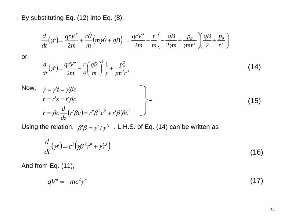
By substituting Eq. (12) into Eq. (8), or, Now, Using the relation, . L.H.S. of Eq. (14) can be written as And from Eq. (11),

qBmm

r

m

Vqrr

dt

d

2

22 222 r

pqB

mr

p

m

qB

m

r

m

Vqr

32

221

42 rm

p

m

qBr

m

Vqrr

dt

d

222 crcrcrdz

dcr

crzrr

cz

3/

rrcrdt

d 22

2mcVq

(14)

(15)

(16)

(17)

32

Substituting (15), (17) into (14)

or after dividing by gives the paraxial ray equation

In non-relativistic limit, we take

32

22

222 1

42 rm

p

m

qBrmc

m

rrrc

22c

022 32222

22

22

rcm

pr

mc

qBrrr

V

V

mc

Vq

V

V

mc

Vq

mc

qV

c

v

2

2

2

2

2

1

22

22

22

22

02842 3

222

mqVr

pr

mqV

Bqr

V

Vr

V

Vr

non-relativistic paraxial equation

(18)

(19)

Eq. 18 is still not a linear

differential equation and it is

not very useful in practice.

33

From Eq. (9),

or,

with initial condition and

22 mr

p

m

qB

22 rmc

p

cm

qB

c

0 0zz

dzrmc

p

cm

qBz

z

020

2

(12)

(13)

34

By substituting Eq. (12) into Eq. (8),

or,

Now,

Using the relation, . L.H.S. of Eq. (14) can be written as

And from Eq. (11),

qBmm

r

m

Vqrr

dt

d

2

22 222 r

pqB

mr

p

m

qB

m

r

m

Vqr

32

221

42 rm

p

m

qBr

m

Vqrr

dt

d

222 crcrcrdz

dcr

crzrr

cz

3/

rrcrdt

d 22

2mcVq

(14)

(15)

(16)

(17)

35

Substituting (15), (17) into (14)

or after dividing by gives the paraxial ray equation

In non-relativistic limit, we take

32

22

222 1

42 rm

p

m

qBrmc

m

rrrc

22c

022 32222

22

22

rcm

pr

mc

qBrrr

V

V

mc

Vq

V

V

mc

Vq

mc

qV

c

v

2

2

2

2

2

1

22

22

22

22

02842 3

222

mqVr

pr

mqV

Bqr

V

Vr

V

Vr

non-relativistic paraxial equation

(18)

(19)

Eq. 18 is still not a linear

differential equation and it is

not very useful in practice.

36

Nonlinear approx. for the angle is

the canonical angular momentum is recalled as .

Four cases are considered:

1. ,

2. ,

3.

4.

if we introduce the magnetic flux

then

dz

rmqV

p

mqV

Bqz

z

022/1

22

028

0A

0A

0A 00

00

rqAmrp 2

0

2

00 mrp

last term of paraxial ray equation vanishes !!

0

00 2

r

Brdr

2

0

qp

(20)

(21)

0A 00

37

We can re-write the last term in the paraxial ray equation as

and

It is sometimes convenient to study the particle trajectories in Larmor frame. The angle

between Larmor frame and the lab frame (r) is given by

The angle L of the particle in the Larmor frame is

When , particle motion in this frame is in a plane through the axis (meridional

Plane). In this case, the trajectory r(z) in the meridional plane may be found from Eq. (18)

alone.

3

2

0

32222

2 1

2

1

rmc

q

rcm

p

32

2

0

3

2 1

8

1

2 rmqV

q

rmqV

p

(relativistic)

(non-relativistic) (23)

(22)

dzm

qBz

zr

0 2

020

dzrmc

pz

zrL

(24)

0p

38

The relativistic paraxial ray equation can be written as

by letting and .

General mathematical properties of Eq. (25) will be discussed in the case

Linear beam optics in an axisymmetric system

In the case of magnetic fields, this description is in the rotating Larmor

frame.

0)()( 21 rzgrzgr

21

zg

22

2

222 c

zg L

(25)

Envelop evolution of a beam with

finite emittance in drift space

39

12 2

11111

2

11 rcrrbra

12 2

22222

2

22 rcrrbra

2/12

111

11

bcaA

2/12

222

22

bcaA

Suppose we have a distribution of particles at some initial position z1 such that

the trace-space area is defined by an ellipse

The area occupied by this distribution at some other point z2 is then found by

solving the transfer matrix relation for (r1,r1’) in terms of (r2,r2’) and substituting in

Eq. (31).

Eq. (32) is still an ellipse since the coefficients are uniquely determined by the

transfer matrix elements and initial coefficients. Emittance of the beam at z1 and

z2 are given by

(31)

(32)

40

An ellipse in x’-y’ plane:

Ellipse in x-y plane:

Where

2

1

22

11

2

1

2

1

W

W

A

A

According to Liouville’s theorem, the emittance are related as

(33)

y’

y

x

x’

12

2

2

2

b

y

a

xbaA

12 22 cybxyax

cossin

sincos

yxy

yxx

2

2

2

2

22

2

2

2

2

cossin

cossinsincos

sincos

bac

bab

baa

2bacbaA

41

At r = rmax, dr/dr’=0. Therefore, by differentiating the ellipse equation, we have

Substituting this result into the ellipse equation, one obtains

For a drift section, the transfer matrix is given by

Rc

bR

cbac

cR

2

c

c

c

bR

2

10

1 zM

12 22 rcrbrar 1~~2~ 22 rcrrbra

22~

~

~

azbzcc

azbb

aa

(49)

42

cc

c

c

cR

42

2

22

43

42

ccc

RR

03

2

R

R

Beam envelope evolution in a drift space

2/1

22

02

0

2

00

2

0 2

zR

RzRRRzR

(50)

(51)

Recall:

21

bac

43

Effects of a Lens on Trace Space Ellipse

and Beam Envelope A distribution of particle with

finite emittance at any location

is represented by an ellipse:

The coefficients a, b, c are

function of z.

The envelop of the beam R can

be defined as the maximum

value of r (or the RMS value of r)

of the beam.

12 22 rcrbrar

How do the trace space ellipse

and beam envelope evolve?

(48)

0

1 2

3

4

x’

x

Uniform Beam Model The beam is assumed to have a sharp boundary

The uniformity of charge and current densities assures that the

transverse electric and magnetic self-fields and the associated

forces are linear functions of transverse coordinates (see below)

This beam model allows us to extend the linear beam optics to

include the space charge forces.

constJ

constinside the boundary

0 J everywhere outside the boundary

a b

beam pipe charged particle beam

evolution of beam envelop

along the propagation

direction is exaggerated!!

• A axisymmetric laminar beam

• Particle trajectories obey

paraxial assumption that the

angle with the z-axis is small.

• The variation of beam radius

along z-axis is slow enough

that Ez and Br can be neglected.

Based on the above assumptions, we have J, and vz v are all

constant values across the beam.

Therefore, with denoting the charge density of the

beam, we obtain

Since we assumed the electric field has only a radial component

and by Gauss’ law,

vaI 2

0 /

va

I

a

IJJ z

20

2

for 0 r a

0 J for r > a

(1)

va

IrrEr 2

00 22

for 0 r a (2a)

vr

IEr

02 for r > a (2b)

the Lorentz force

exerted on an electron

in the beam has radial

component only and is

a linear function of r.

The magnetic field, on the other hand has only an azimuthal component,

is obtained by applying Ampere’s circuital law:

20

2 a

IrB

r

IB

20

for 0 r a

for r > a

(4)

2

2

ln21a

r

a

bVr s for 0 r a

r

bVr s ln2 for r > a

(5)

Integrate the electrostatic field along an arbitrary path from r = a to r = b,

IIaVs

30

44 00

2

0 (6)

by setting that = 0 at r = b, where The peak potential on the beam axis (r =

0) is thus . And

the maximum electric field at the beam

edge is

aI

a

VEa /60

2

abVV s ln210 0

The motion of a beam particle in such field is described by the radial force equation

BvEqrmrmdt

dzr

where we dropped the force term that is negligibly small and

because there is no external acceleration. zBqr r .const

Substitution for Er from the first equation of (2), B from the first equation of (3)

and with , , we have 2

00

c cvz

(8)

2

2

0

12

ca

qIrrm (9)

with rcdz

rdvr z

22

2

22 we have

(10) 3332

02 mca

qIrr

Define characteristic current (Alfve’n current) I0 as

q

mc

q

mcI

23

00

30

14

which is approx. 17 kA for electrons and 31 (A/Z) MA for ions of mass number A

and charge number Z.

(11)

Define “generalized perveance” K such that

33

0

2

I

IK

In terms of generalized perveance, the equation of motion can be expressed as

(12)

ra

Kr

2

Under the condition of laminar flow, the trajectories of all particles are similar

and scale with the factor r/a. That is, the particle at r=a will always remain at the

boundary of the beam. Thus, by setting r = a = rm, we obtain

Krr mm

(13)

(14)

022 332

2

32222

22

22

mm

n

m

mmmmr

K

rrcm

pr

mc

qBrrr

From the paraxial ray equation and considering the effects of finite emittance and

linear space charge, we obtained the beam envelop equation:

(15)

Vlasov Model Describe the self-consistent beam motion under the

action of electromagnetic fields

When the effect of the velocity spread is not negligible

(compared with that of self-fields), the flow is then non-

laminar.

A system of identical charged particles is defined by a

distribution function f(qi, pi, t) in 6D phase space.

Beam EM fields

Self fields Applied fields

Vlasov equation

Recall Liouville’s theorem:

The phase-space coordinates qi, pi follows Hamiltonian equations of

motion:

where H is the relativistic Hamiltonian, that is

and A are the scalar and vector potentials of the EM

fields, which is applied fields + self-fields. The self-field

contributions are determined by the charge and current

densities via the wave equations:

03

1

i

i

i

i

i

pp

fq

q

f

t

f

dt

df

,i

ip

Hq

i

iq

Hp

qAepcmctpqH ii 2/1222,,

volume occupied by a

number of particles N

in phase space is constant

.33 constpqdd

,0

2

2

00

2

tJ

t

AA

02

2

00

2

In terms of space coordinates and mechanical momentum Pi=pi-qAi,

and if the distribution function f=f(qi,Pi,t)) in (qi,Pi) phase space

satisfies Liouville’s theorem. That is:

.33 constPqdd

03

1

i

i

i

i

i

PP

fq

q

f

t

f

dt

df or

but BvEqP

Lorentz force law

we have

03

1

i i

ii

i P

fBvEqq

q

f

t

f

relativistic Vlasov equation

.3333 constPqddpqdDd

ii

ii

Pq

pqD

,

,

In Vlasov beam model, one has to solve the following equations self-

consistently (Maxwell-Vlasov equations):

03

1

i i

ii

i P

fBvEqq

q

f

t

f

0

,,

,,

3

0

00

3

0

B

PdtPqfq

E

t

EPdtPqfvqB

t

BE

ii

ii

2/1

22

2

1

cm

P

m

Pv

• Vlasov equation is, in

general, nonlinear.

• given a initial beam

distribution,

integrate Vlasov

numerically.

• determine an

equilibrium state,

linearize Vlasov

equation w.r.t. this

state and solve the

linearized equation

for small signals.

Equilibrium States of a Distribution of

Particles

03

1

i i

ii

i P

fBvEqq

q

f

0

,,

,,

0

3

0

3

0

B

PdtPqfq

E

PdtPqfvqB

E

ii

ii

usual approach is to choose

a distribution function that

depends on the constants of

motions. That is

with and Ijs are

constants of motion

0

dt

dI

I

f

dt

df j

j j

jIff

Linearization of Vlasov Equation

Let the equilibrium distribution function be f0 and consider a small

perturbation on f1 on the equilibrium state. i.e.

and now f1 satisfies

but now the EM fields are small associate with the perturbation f1.

we can now assume that these quantities are small perturbations

from steady state. Solving the linearized Vlasov equation allows us

to study system stability (instabilities).

tPqfftPqf iiii ,,,, 10

03

1

111

i i

ii

i P

fBvEqq

q

f

t

f

Electron Beam Injectors for Free

Electron Lasers

Photo-injector for XFEL

The SACLA pulsed thermionic DC gun injector

The NSRRC Photo-injector System

The Accelerator Test Area @ NSRRC

SRF Gun System @ Helmholtz-Zentrum Rossendorf

APEX: the high repetition-rate photo-cathode

rf gun at LBNL