basics of detection and estimation theory … of detection and estimation theory in this chapter we...
TRANSCRIPT
83050E/158
BASICS OF DETECTION AND ESTIMATION THEORY In this chapter we discuss how the transmitted symbols are detected optimally from a noisy received signal (observation). Based on these results, optimal receiver structures are later developed for the modulation methods presented earlier. The same theoretical framework is the basis for optimal solutions for the following problems:
1. Symbol detection from a received noisy continuous-time signal, or from the corresponding discrete-time sample sequence.
We consider first the simplified case of detecting an isolated symbol in case of an AWGN channel model.
Then symbol sequence detection in case of an ISI channel is considered.
2. Decoding of error correction codes.
3. Parameter estimation, like estimating the signal amplitude, carrier phase, symbol timing, and other synchronization parameters of the receiver.
The Viterbi algorithm is a commonly used efficient implementation algorithm for the optimal sequence detection principle. Source: Lee&Messerschmitt, Chapter 7.

83050E/159
Terminology and System Model Here we consider mostly a discrete-time system model. The term estimation is used when we want to know the value of a continuous variable.
The term detection is used when we want to decide which of possible values from a discrete set of values is the correct one. The system model includes two aspects:
o Signal generation model: Deterministic processing of the signal, like coding, modulation, filtering.
In theoretical considerations, the channel response is assumed to be known through channel estimation, so for example, the ISI produced by multipath channel belongs to the signal generation model.
o Noise generation model: Random, usually additive noise/distortion effects. We consider in the continuation two main cases:
Random bit errors produced by a binary symmetric channel (BSC) to a bit sequence.
Additive Gaussian noise.
SIGNAL GENERATIONMODEL
NOISE GENERATIONMODEL
INPUT OBSERVATION
Xk Yk There are two general detection/estimation principles:
ML = maximum likelihood MAP = maximum a-posteriori.

83050E/160
Detection of an Isolated Real-Valued Symbol Based on a Discrete-Valued Observation The receiver makes a decision about the transmitted symbol A based on an observation Y . The input is a symbol A, randomly chosen from the alphabet
AΩ . The output Y is a discrete-valued random variable, which is distorted due to noise generation. The system is described by the conditional probabilities )ˆ( ayp AY . An ML detector chooses the symbol Aa Ω∈ˆ which maximises )ˆ( ayp AY when there is the observation y from the output Y . A MAP detector maximises the a-posteriori probability
)ˆ( yap YA . The latter criterion is intuitively better. As will be seen shortly, it also minimizes the error probability.

83050E/161
About ML and MAP Detection Based on the Bayes rule, the ML and MAP detectors are related through
)(
)ˆ()ˆ()ˆ(
yp
apaypyap
Y
AAYYA =
In MAP detection, it is sufficient to maximize the numerator, since the denominator is invariant in the maximization. So, to be able to do MAP detection, the symbol probabilities )(⋅Ap must be known. In the important special case that the symbols are equally probable, the MAP detector is equivalent to the ML detector. The ML detector is easier to implement than the MAP detector, and it is commonly used in practise. Also the symbol probabilities are usually equal. The transmitter may include a special function (scrambling or energy dispersal) to satisfy this requirement. In some cases the symbol probabilities might not be known, but it is sensible to assume them to be equally probable.

83050E/162
About the Optimality of MAP Detection
In general, the probability of correct decision can be written as
[ ] [ ]
)()ˆ(
)(PrPr
ypyap
ypyYdecisioncorrectdecisioncorrect
Yy
YA
Yy
Y
Y
∑=
∑ ==
Ω∈
Ω∈
Since the probabilities )( ypY are always non-negative, this sum is maximized when each of its terms is maximized. And this is exactly what a MAP detector is doing. So we can say: The MAP detector minimizes the error probability. As mentioned earlier, in most practical cases the symbol probabilities are equal, and in these cases also the ML detector minimizes the error probability.

83050E/163
An Example about ML and MAP Detection (a) Equally probable symbols
5.0)12( 0)02(
5.0)11( 5.0)01(
0)10( 5.0)00( 2,1,0
tindependen are and 0.5=(1)=(0) 1,0 0.5=(1)=(0) 1,0
==
==
==
∈⇒
∈∈+=
AYAY
AYAY
AYAY
NN
AA
pp
pp
ppy
NAppnppa
NAY
An ML detector makes the decisions as follows:
1ˆ 2 randomly) (e.g. 1ˆor 0ˆ 1
0ˆ 0
=⇒===⇒=
=⇒=
ayaay
ay
Since the symbols are equally probable, the MAP detector works in the same way (b) Case with different symbol probabilities p pA A(0) = 0.75 (1) = 0.25 An ML detector works as before.
In the cases of and yy = 0 = 2 the MAP detector works as above, but in the case of y there is a difference. The a-posteriori-probabilities are
= 1
25.0)11( 75.0)10( == YAYA pp
so the MAP detector chooses now a = 0 when y = 1.

83050E/164
An Example about ML and MAP Detection (cont.) The error probabilities can be evaluated as follows: (a) ML and MAP detection work in the same way:
0.25y probabiliterror average
0y probabiliterror 0.25;y probabilit with20.5y probabiliterror 0.5;y probabilit with1
0y probabiliterror 0.25;y probabilit with0
⇒
===
yyy
(b) In cases of y or y no errors. = 0 = 2
ML: 0.25y probabiliterror average
0.5y probabiliterror 0.5;y probabilit with 1y⇒=
MAP: 0.125y probabiliterror average
0.25y probabiliterror 0.5;y probabilit with 1y⇒=
So we can see that the MAP detector works clearly better in this situation.

83050E/165
Binary Symmetric Channel, BSC The BSC model is commonly used in error control coding studies.
x=0
x=1
y=0
y=1
p y x pY X* ( )=1* −
1−p
p
Binary symbols are transmitted: qpqp AAA −===Ω 1)1( ,)0( ,1,0
ML detector assuming 5.0<p :
[ ] perrorya
==
Prˆ
MAP detector: Case : 0=y
⎩⎨⎧
<>
=⇒−=−=pqpq
apqppqp YAYA if 1 if 0
ˆ)1()01()1()00(
Case 1=y :
⎩⎨⎧
>+<+
=⇒−−==1 if 01 if 1
ˆ)1)(1()11()10(pqpq
apqpqpp YAYA

83050E/166
Detecting a Single Real-Valued Symbol Based on a Continuous-Time Observation The observation is now Y A N= + where N is an additive continuous-valued noise sample. The Bayes rule can now be written as:
)(
)ˆ()ˆ()ˆ(
yf
apayfyap
Y
AAYYA =
where fY A ( )⋅ ⋅ and fY ( )⋅ are now continuous probablility distributions. ML and MAP detection are defined in the same way as earlier.
83050E/167
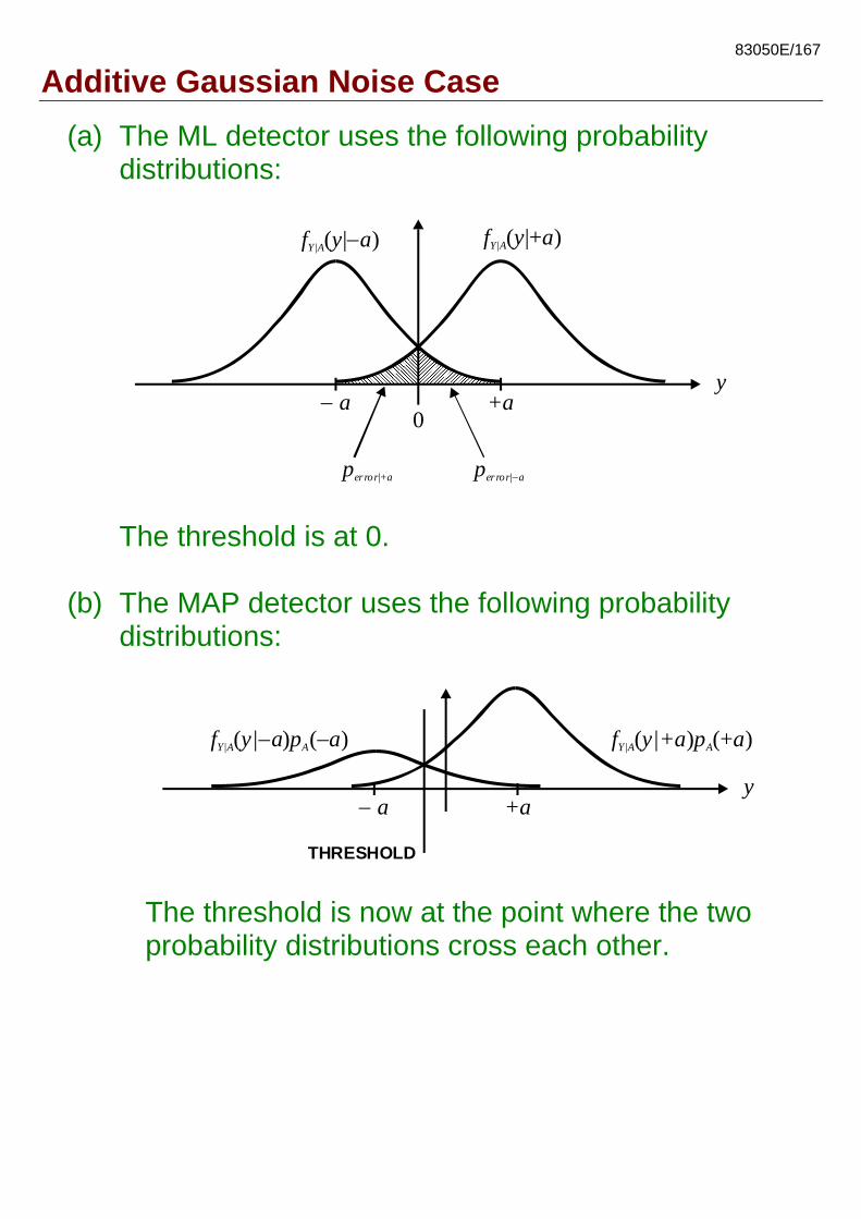
Additive Gaussian Noise Case (a) The ML detector uses the following probability
distributions:
y
f y aY|A( |+ )
0− a
perror a|+ perror a|−
+a
f y aY|A( | )−
The threshold is at 0.
(b) The MAP detector uses the following probability distributions:
y
f y| a p aY|A A( ) ( )− − f y|+a p aY|A A( ) (+
THRESHOLD
)
+a− a
The threshold is now at the point where the two probability distributions cross each other.

83050E/168
Another Example with Uniform Noise PDF
NAYpp AAA
+==+=−−=Ω 75.0)1( ,25.0)1( ,1,1
N has uniform distribution:
−1.5 1.5
f nN ( )
n
1/3
MAP detector compares the following probability functions:
−1 1
f nN ( )
1/121/4
n
fN(n)
In the range it chooses 5.05.0 <<− y 1ˆ =a . The threshold is at 0.5. The error probability is 1/12. ML detector compares the following probability functions:
−1 1
1/3 1/3
n
In the range it chooses (e.g. randomly) either of the two symbols. Or it may set a threshold somewhere in this range. Depending on the chosen threshold,
5.05.0 <<− y
1/12 < error probability<1/3.

83050E/169
Detecting a Signal Vector In the following, we consider detecting a sequence of symbols optimally, taking eventually into account also the intersymbol interference. We consider the symbol sequence as a vector-valued symbol, which can be detected using the ML or MAP principles. A simple example of vector-valued signal is an I/Q symbol in baseband format, the real and imaginary parts being the elements of the vector. But in the following, the vector elements are the (real- or complex-valued) symbols of a finite-length symbol sequence. We can denote the signal vector as
S=[A1, A2, A3, … , AM]
where M is the number of symbols in the vector. Any transmission link can be considered as a vector channel using the following model:
VECTOR TOSCALAR
CONVERTERSCALAR
CHANNELSCALAR TO
VECTORCONVERTER
NOISESYMBOLS OBSERVATION
EQUIVALENT VECTOR CHANNEL The vector dimensionality may be defined by the application in a natural way, but in other cases it can be chosen freely for analysis purposes.

83050E/170
Detecting a Signal Vector (continued)
In case of signal vector detection, the observation vector has the same dimensionality as the signal vector. The noise process is determined by the conditional probability distributions
fY S y s( ). The noise components of the observation vector are usually assumed to be independent (in the Gaussian case, this is satisfied if the components are white,i.e., uncorrelated). In this case we can write
∏==
M
kkkSY syff kk1
)( )(sySY
ML-detection selects the symbol vector s that maximizes the conditional probability
ˆ)ˆ( sySYf . As earlier, the statistics of
the transmitted signals needs not be taken into account.

83050E/171
ML-Detection in Case of Additive Gaussian Noise
Assuming additive Gaussian noise with variance σ2 and with uncorrelated samples, we can write the conditional probability as
⎥⎦⎤
⎢⎣⎡ −−=
−=−=
222/ ˆ
21
exp)2(
1)ˆ()ˆˆ()ˆ(
sy
syssysy SSY
σσπ MM
NN fff
ML-detector chooses the vector s that maximizes the above function. This is clearly equivalent to minimizing the Euclidean distance
sy ˆ−
(or equivalently the squared Euclidian distance sy ˆ− 2) In the additive Gaussian noise case, ML-detector chooses the signal vector s that is closest to the observation vector
using the Euclidean distance measure. This will be the leading principle in the following !
ˆy
The elements of the signal vector may be also complex-valued. The (squared) Euclidean distance measure to be minimized can be written as 2 2
1 1ˆ ˆ ˆ 2M My s y s− = − + + −y s

83050E/172
ML-Detection in Case of BSC
s=0
s=1
y=0
y=1
p y s pY S* ( )=1* −
1−p
p
In this case, the elements of the signal vector and the observation vector are binary-valued.
The conditional probabilities in the BSC case are
ˆ
ˆ1 ˆk k
k kk kY S
k k
p yp y s
p yss
≠⎧= ⎨ − =⎩
( )
Definition: The Hamming distance ),ˆ( ysHd of two (equal-length) binary vectors s and ˆ y is equal to the number of elements where the vectors differ from each other.
Now we can write the conditional probability for the binary signal vector of length M as (independence assumption !) ),ˆ(),ˆ( )1()ˆ( ysys
SY sy HH dMd ppp −−= . This is the probability for the case that the differing bits have been changed by that channel, but the others not.
In practice, 5.0<p and the ML-detector minimises ),ˆ( ysHd . In the BSC case, ML-detector chooses the signal vector s that is closest to the observation vector using the Hamming distance measure.
ˆy

83050E/173
About ML-Detection in the AWGN and BSC Cases
In ML detection, basically the same rule is used in both of the previously discussed cases: The signal vector that is closest to the observation vector is chosen. The only difference is the used distance measure, either Euclidean or Hamming. In both cases, the set of possible observation vectors can be divided into decision regions, which include the possible observation vectors that are closest to each of the signal vectors. The earlier presented rule for detecting PAM/QAM/PSK symbols in case of ISI-free channel is one important case of this general criterion.
83050E/174
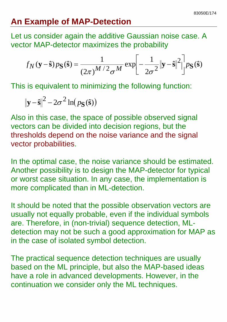
An Example of MAP-Detection Let us consider again the additive Gaussian noise case. A vector MAP-detector maximizes the probability
)ˆ(ˆ2
1exp)2(
1)ˆ()ˆ( 222/ ssyssy SS ppf MMN ⎥
⎦
⎤⎢⎣
⎡−−=−
σσπ
This is equivalent to minimizing the following function:
( ))ˆ(ln2ˆ 22 ssy Spσ−−
Also in this case, the space of possible observed signal vectors can be divided into decision regions, but the thresholds depend on the noise variance and the signal vector probabilities. In the optimal case, the noise variance should be estimated. Another possibility is to design the MAP-detector for typical or worst case situation. In any case, the implementation is more complicated than in ML-detection. It should be noted that the possible observation vectors are usually not equally probable, even if the individual symbols are. Therefore, in (non-trivial) sequence detection, ML-detection may not be such a good approximation for MAP as in the case of isolated symbol detection. The practical sequence detection techniques are usually based on the ML principle, but also the MAP-based ideas have a role in advanced developments. However, in the continuation we consider only the ML techniques.

83050E/175
Error Probability Evaluation: (i) Two Signal Vectors, Gaussian Noise
Let us consider first the case of two M -dimensional signal vectors, and . is js The noise produces an M -dimensional vector N , the elements of which are zero-mean Gaussian-distributed random variables, the variance of which is 2σ . A sequence detection error occurs if isS = is transmitted and is detected. jss =ˆ To simplify notation, we can assume the special case with
and . Assume now that 0s =i qs =j 0s =i is transmitted, thus the received vector NN0Nsy =+=+= i . An error occurs if
22 0yqy −<− or if 22 0NqN −<− . This is equivalent to 22
122
11 )()( MMM NNqNqN ++<−++− or
2
221
11M
MMqqNqNq ++
>++ .
In vector form this can be expressed as:
22
22 d=>′ q
Nq
where is the Euclidean norm of q. d

83050E/176
Error Probability Evaluation: (i) Two Signal Vectors, Gaussian Noise (continued)
Above is a linear combination of independent Gaussian variables, and thus it has the variance
Nq′
( ) 222221 σσ dqq M =++
The error probability becomes
⎥⎦⎤
⎢⎣⎡=
⎥⎥⎦
⎤
⎢⎢⎣
⎡
σσ 22/2 dQ
ddQ
The error probability of binary PSK derived earlier is a special case of this. This result can be generalized for two arbitrary vectors: If the observation vector is NsY += i , where the elements of the noise vector N are zero-mean Gaussian random variables with variance 2σ , then the error probability is given by
[ ] ⎥⎦⎤
⎢⎣⎡=−<−σ2
Pr dQij sYsY
where d is the Euclidean distance of the two vectors,
jss −= id .

83050E/177
Error Probability Evaluation: (ii) Two Signal Vectors, BSC
Now we consider the case of two M -dimensional binary signal vectors, and that have a Hamming distance of
, i.e., they differ in bits. is js
d d The conditional probabilities are now of the form:
),ˆ(),ˆ( )1()ˆ( ysysSY sy HH dMd ppp −−= .
When is transmitted, ML-detector chooses if is js
),(),( ysys iHjH dd ≤
Further it is assumed that in a boarder case (with same distance to both signal vectors), the detector always makes the wrong decision. We can also note that errors in those bits where the two signal vectors are the same do not matter. A sequence detection error occurs if there are more than t errors in those bits, where and differ. Here is js t is largest integer for which dt <2 , i.e.,
⎩⎨⎧
−−
=even 12/
odd 2/)1(dddd
t

83050E/178
Error Probability Evaluation: (ii) Two Signal Vectors, BSC (continued)
Now the error probability can be written as:
( ) idid
ti id
pppdQ −
+=⎟⎠
⎞⎜⎝
⎛ −∑= )1(,1
Here, this Q-function is based on the binomial probability distribution. The result is similar to the additive Gaussian noise case, now only the Q-function is based on a different probability distribution. Example: Let . [ ] [110111 ,000000 == ji ss ] Here the Hamming-distance is 5. A detection error occurs if there is an error in at least three of the five bits that are different in the two signal vectors. The error probability is
( )
51423
51423
)1(5)1(10
55
)1(45
)1(35
,5
ppppp
ppppppQ
+−+−=
⎟⎠
⎞⎜⎝
⎛+−⎟
⎠
⎞⎜⎝
⎛+−⎟
⎠
⎞⎜⎝
⎛=

83050E/179
Error Probability Evaluation: (iii) Many Signal Vectors Now there are K signal vectors, Kss ,,1… in use. We assume that is transmitted and the observation vector is
. Let represent the error case where the observation is closer to than .
isY jE
js is With K=3, the error probability can be written as [ ] [ ] [ ] [ ]32321 PrPrPr Pr EEEEdtransmitteerror ∩−+=s . In practise, we can ignore the last term that has only a minor effect. In the general case, we obtain an upper bound using the union bound principle as:
[ ] [ ]∑≤
≠=
K
ijj
ji Edtransmitteerror1
Pr Pr s
On the other hand, the most probable error event, , gives a (rather tight) lower bound:
maxE
[ ] [ ]maxPr Pr Edtransmitteerror i ≥s

83050E/180
Error Probability Evaluation: (iii) Many Signal Vectors (continued)
The following approximation, which depends on the minimum distance, , is commonly used: mind
[ ] [ ]maxPr Pr Edtransmitteerror i ≈s
where
[ ][ ] case BSCfor ),(Pr
casenoiseGaussian additivefor )2/(Pr
minmax
minmaxpdQE
dQE== σ
The overall average error probability is obtained as a weighted average of the error probabilities of the different signal vectors (weighted by the probabilities of the signal vectors). Usually, the different signal vectors are equally probable, and the overall error probability is given by
[ ] [ ]dtransmitteerrorerror i PrPr s= .
So we have obtained lower and upper bounds, and an approximative formula for the error probability in vector detection. The BSC case and the additive Gaussian noise case can be handled using very similar principles. The error probability depends essentially on the minimum distance and noise variance !
83050E/181
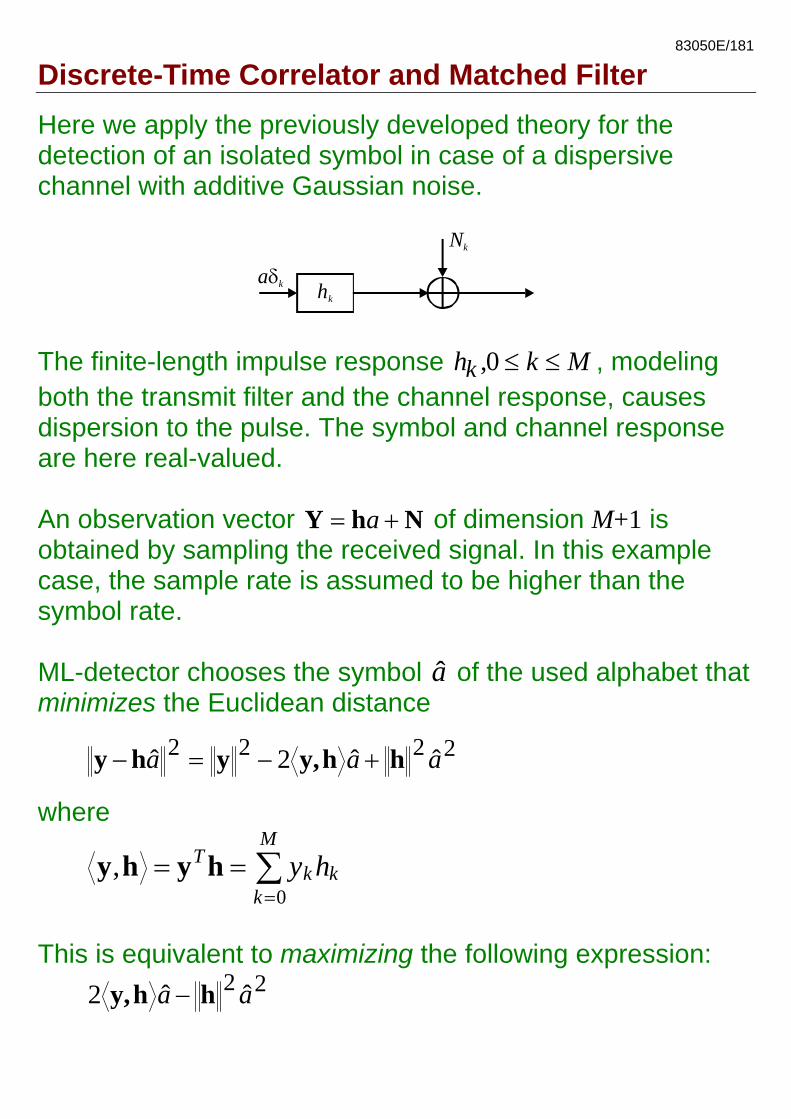
Discrete-Time Correlator and Matched Filter Here we apply the previously developed theory for the detection of an isolated symbol in case of a dispersive channel with additive Gaussian noise.
hk
aδk
Nk
The finite-length impulse response Mkhk ≤≤0, , modeling both the transmit filter and the channel response, causes dispersion to the pulse. The symbol and channel response are here real-valued. An observation vector NhY += a of dimension M+1 is obtained by sampling the received signal. In this example case, the sample rate is assumed to be higher than the symbol rate. ML-detector chooses the symbol of the used alphabet that minimizes the Euclidean distance
a
2222 ˆˆ2ˆ aaa hhy,yhy +−=−
where
∑=
==M
kkk
T hy0
, hyhy
This is equivalent to maximizing the following expression: 22 ˆˆ2 aa hhy, −

83050E/182
Discrete-Time Correlator and Matched Filter (cont’d)
The first term can be calculated using a correlator:
∑==
M
kkk hy
0,hy
hk
Σyk < >y h,
or, equivalently, using a matched filter:
000
,==
−=
⎟⎟⎠
⎞⎜⎜⎝
⎛∑=∑=
n
M
kknk
M
kkk hyhyhy
< >y h,h−k
yk
k=0 The impulse response of the matched filter is the mirror image of the received pulse shape in case of real signals (or complex conjugate mirror image in case of complex channel model.) We see here the equivalency of correlation receiver and matched filter receiver as optimum receiver principles. The equivalency is due to the close relation between correlation and convolution operations. These principles will be discussed further later on.
83050E/183
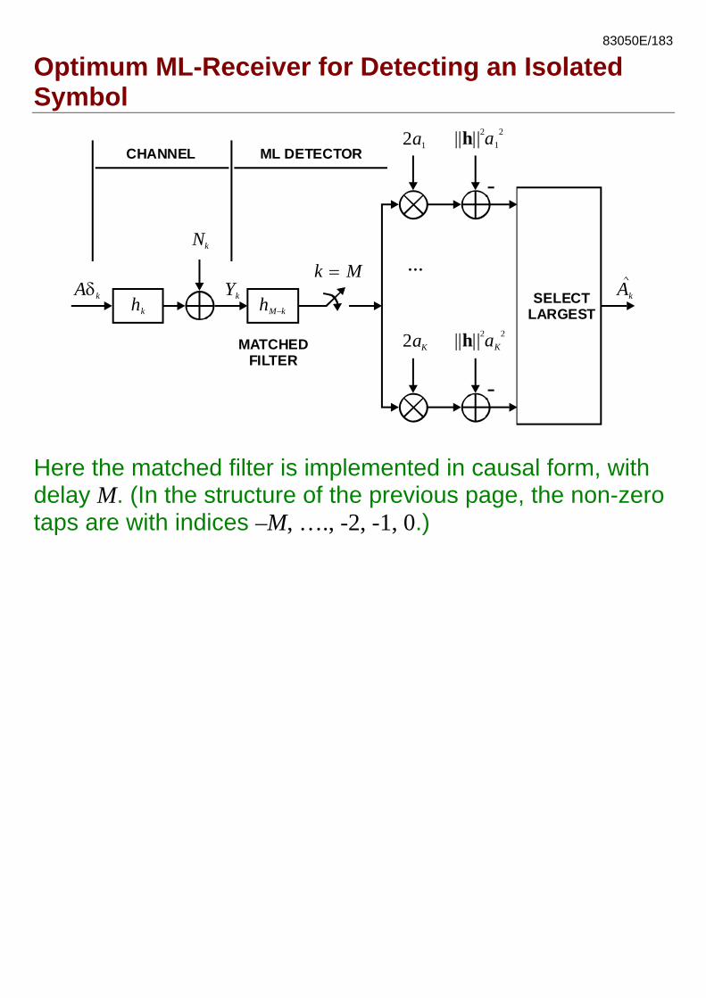
Optimum ML-Receiver for Detecting an Isolated Symbol
hM k−
Ykhk
Aδk
...SELECT
LARGESTAk
2a1 || ||h 2 2a1
2aK || ||h 2 2aK
CHANNEL ML DETECTOR
MATCHEDFILTER
k M =Nk
Here the matched filter is implemented in causal form, with delay M. (In the structure of the previous page, the non-zero taps are with indices –M, …., -2, -1, 0.)
83050E/184
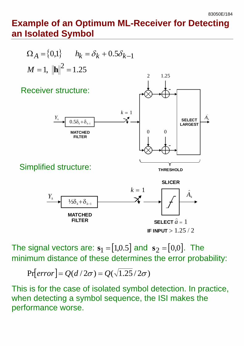
Example of an Optimum ML-Receiver for Detecting an Isolated Symbol
0.5δ +δk k 1−
Yk SELECTLARGEST
Ak
2 1.25
0MATCHEDFILTER
k = 1
0
THRESHOLD
25.1 ,1
5.0 1,02
1
==
+==Ω −
hM
h kkkA δδ
Receiver structure:
Simplified structure:
½δ +δk k 1−
Yk
MATCHEDFILTER
k = 1Ak
SLICER
SELECT a = 1IF INPUT > / 1.25 2
The signal vectors are: [ ]5.0,11 =s and [ ]0,0 2 =s . The minimum distance of these determines the error probability:
[ ] )2/25.1()2/(Pr σσ QdQerror ==
This is for the case of isolated symbol detection. In practice, when detecting a symbol sequence, the ISI makes the performance worse.

83050E/185
About Markov Chains
A Markov chain kΨ is a discrete-time and discrete-valued random process that satisfies the condition:
)(),,( 111 kkkkk pp ΨΨ=ΨΨΨ +−+ …
kΨ is the state of the Markov chain at time k . It depends only on the previous state. Markov chains are used, e.g., to model finite state machines with random inputs. In the following, they are used as the signal generation model for ISI channels, and later for modeling certain type of coding methods. A Markov chain is homogenous if the conditional probability
)( 1 kkp ΨΨ + does not depend on k . In this case, the system is in a way stationary or time-invariant. The properties of homogenous Markov chains are determined by the state transition probabilities
)()( 1 ijpijp kk ΨΨ += .

83050E/186
Shift Register Process as a Markov Chain Shift register process:
Xk
z−1 z−1 z−1 z−1Xk−1 Xk−2 Xk M−...
Ψk
Here kX is a discrete-valued random variable, which is independent of the variables 1, ,k kX X M− −… . The state is defined as:
Mkkk XX −−=Ψ ,,1 … .
It can be shown that such a system satisfies the Markov condition. This is a vector-valued Markov chain.

83050E/187
Using Shift Register Process to Model ISI Channels
Let us consider the detection of a symbol vector (or symbol sequence) in a case of a channel that has ISI. The ISI is defined by the symbol-rate channel impulse response hk .
Nk
Ykhk
skak A signal with ISI can be modeled as a homogenous Markov chain, using the shift register process:
Xk z−1 z−1 z−1 z−1...
Ψk
h X X g( )= (Ψ Ψ )k k M k k, , ,− +1... NOISE
GENERATIONMODEL
YkSk
The state is defined by the contents of the delay line,
Mkkk XX −−=Ψ ,,1… , and the output of the signal generation model can be formulated as ),( 1+ΨΨ= kkk gS , where g( , )⋅ ⋅ is a memoryless function. The random variables are independent and identically distributed.
iX
The impulse response kh is usually finite in length and then
∑==
−M
iikik XhS
0As usual, the additive noise is assumed to have independent samples.

83050E/188
Example of ISI Channel We consider a continuous-valued channel with impulse response
15.0 −+= kkkh δδ
This has the following Markov chain model (left part):
Xk=Ak
z−1Xk−1=Ak−1
Sk
Nk
Yk
h X X X X( )= +k k k k, − −1 10. 5
10
( )1, 1
( )0, 0 ( )1, 1.5
( )0, 0.5
INPUT OUTPUT
Here the state is the previous transmitted symbol Ak–1. On the right, a corresponding state transition diagram for the system is given. The arcs are labeled with noise-free input/output pairs (Ak / Sk). In other words, each node of the diagram corresponds to a state of the Markov chain. The noise-free input and output values of the signal generation model are shown for each branch (state transition) of the diagram.
83050E/189
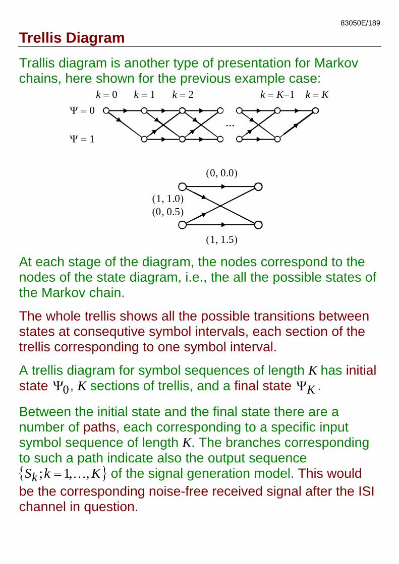
Trellis Diagram Trallis diagram is another type of presentation for Markov chains, here shown for the previous example case:
Ψ = 0
Ψ = 1
k 0= k 1= k 2= k K 1= − k K =
...
( )0, 0.0
( )1, 1.0(0 ), 0.5
( )1, 1.5
At each stage of the diagram, the nodes correspond to the nodes of the state diagram, i.e., the all the possible states of the Markov chain.
The whole trellis shows all the possible transitions between states at consequtive symbol intervals, each section of the trellis corresponding to one symbol interval.
A trellis diagram for symbol sequences of length K has initial state , K sections of trellis, and a final state 0Ψ KΨ .
Between the initial state and the final state there are a number of paths, each corresponding to a specific input symbol sequence of length K. The branches corresponding to such a path indicate also the output sequence KkS k ,,1; …= of the signal generation model. This would be the corresponding noise-free received signal after the ISI channel in question.

83050E/190
Sequence Detector Continuing the previous continuous-valued, additive Gaussian noise case, the observed sequence at the detector would be kkk NSY += . A sequence detector aims at determining the transmitted symbol sequence based on such an observation. When doing the detection, the signal generation model is assumed to be completely known; in practical systems the ISI channel must somehow be estimated to be able to utilize the idea. According to the ML vector detection principle, one should choose the sequence that is closest to the observed sequence according to proper metric, i.e., the Euclidean metric in our example case.
The candidate sequences are the sequences produced by the signal generation model as responses to all the possible symbol sequences (with the used alphabet) of length K. For each possible symbol sequence, there is a unique path through the trellis, and the corresponding ideal sequence, produced by the signal generation model, is determined by the path. Thus, the ML vector detection problem is equivalent to finding the path through the trellis that is closest to the observed sequence according to the used metric !

83050E/191
Sequence Detector (continued)
Given an observed sequence, a path metric is defined for each path through the trellis. It is the distance between the corresponding ideal sequence and the observed sequence, using the relevant metric. Each section of the trellis corresponds to one symbol interval, with observed sample ky .The brach metric is defined for each branch j of each section k as
⎪⎩
⎪⎨
⎧
−
−
case BSC )(
case noiseGaussian additive 2
jkkH
jkk
syd
sy
A path metric is obtained by adding up the branch metrics corresponding to the path. An ML sequence detector could be realized by
- Calculating all the branch metrics. - Calculating all the path metrics out of the branch
metrics. - Finding out the path with the smallest path metric. - The symbol sequence corresponding to this path is the
optimally detected sequence accoring to the ML vector detection principle.
However, such a scheme would be very complicated to implement for long symbol sequnces.

83050E/192
Viterbi Algorithm Basically, Viterbi algorithm is an application of dynamic programming to solve the previously described path minimization problem efficiently. The principle is as follows:
(1) The trellis is examined section by section, starting from the initial stae and ending at the final state.
(2) At the beginning of each phase, the shortest paths (surviving paths) from the initial node to the input nodes of the section under examination are known. Then the shortest paths from the initial node to all the output nodes of the section are searched. They are found by calculating the path metrics of all possible combinations of surviving paths and branches of the current section, and choosing the shortest path to each output node.
(3) This is continued until we reach the final state. At this point, only one path is surviving, and this corresponds to the detected sequence.
At each stage, there are N surviving paths, where N is the number of parallel states in the trellis, i.e., the number of states in the Markov model. The Viterbi algorithm is based on the following property: If the shortest path goes through node x, then the metric of this path is the sum of the two shortest paths, one from initial node to x and one from x to final node.

83050E/193
An Example of Viterbi Algorithm We continue the previous example with signal generation model
15.0 −+= kkkh δδ
and additive Gaussian noise. We assume that the received sequence is 0.2, 0.6, 0.9, 0.1. The following trellis diagram shows all the branch metrics. Then the surviving paths are shown for each phase of the Viterbi algorithm.
Ψ = 0
Ψ = 1
k 0= k 1= k 2= k 3= k 4=0.04 0.36 0.81 0.01
0.160.01
0.64 0.010.16
0.16
0.810.6
0.360.9OBSERVATIONS: 0.2
0.1
TRELLIS (ALL PATHS SHOWN):
0.04
0.64
0.04
0.64
0.360.04
0.160.01
0.400.65( )
0.201.45( )0.81
0.64PATH METRIC
BRANCH METRIC
VITERBI ALGORITHM (ONLY SURVIVORS ARE SHOWN):
0.360.04
0.16 0.010.16
0.36
0.410.04
0.160.16
0.010.37
1DECISION: 0 0
0
83050E/194
An Example of Viterbi Algorithm (continued) So the Maximum Likelihood Sequence Detection (MLSD) gives as the detected symbol sequence 0, 1, 0, 0, whereas a simple symbol-by-symbol slicer ignoring the ISI would give 0, 1, 1, 0. The knowledge of ISI if present is, of course, useful !

83050E/195
About the Viterbi Algorithm During the processing of each section of the trellis (except for the first and last sections), a constant amount of computation is carried out. So the computational complexity is proportional to the sequence length K. In the presented form, the Viterbi algorithm gives the detected sequence after all the sections have been processed. Partial detection of the first symbols before the final result often takes place (like in the previous example), but is never guaranteed. This could introduce excessive detection delays when detecting a long sequence. This can be avoided by defining truncation depth, d, such that when processing section k, possible parallel surviving paths starting earlier than section k-d are removed by keeping only the shortest of those paths. This means that the maximum detection delay is d symbols. Choosing the trunction depth large enough, the detection performance is not significantly degraded. In this way, the Viterbi algorithm can be used even for infinitely long symbol sequences. Viterbi algorithm can be used for all ML and MAP detection problems, where the signal generation can be modelled as a homogenous Markov chain. Important special cases include: • Detection after a channel with ISI and additive Gaussian
noise. • Decoding of certain error control codes (convolution
codes and trellis codes to be discussed later).

83050E/196
Evaluation of Error Probabilities In case of Viterbi detection/decoding, we can talk about an error event, which means single ‘detour’ of the detected path outside the right path. The length of an error event is the number of wrong nodes, or number of trellis sections with wrong path –1. As an example, error events of lengths 1 and 2:
In this context we can talk about detection errors. In sequence detection, a detection error may produce several symbol errors, an error burst, the length of which depends on the length of the error event. The detection error probability can be evaluated using the earlier formulas for ML sequence detection:
BSCforpdKQ
channelsnoiseGaussianadditivefordKQ),(
)2/(
min
min σ
Here K is a coefficient that is not very easy to be determined but can often assumed to be 1, and dmin is the minimum distance, i.e., the shortest distance between the right path and the ‘detour’, over all possible error events. Notice that in this context, the path lengths are calculated using the branch values corresponding to the ideal signal generation model, not using the actual branch metrics used in detection.

83050E/197
Evaluation of Error Probabilities (continued)
Example: In the example case considered earlier in Viterbi detection, the shortest error events are:
0 0
1.0 0.25
0 0 0
1.0 0.252.25
The length 1 and 2 error events have the following distances, respectively: 25.15.01 22 =+ 5.35.05.11 222 =++ So the minimum distance in this example is 25.1min =d This can be verified by checking all the (short) error events. The minimum distance in this example is, more or less by change, equal to the minimum distance in isolated symbol detection with the same channel, that was discussed earlier. However, with ISI channels, the performance in sequence detection is usually much worse than in isolated symbol detection. In sequence detection, it is usually not easy to find the minimum distance by inspection. However, a modification of the Viterbi algorithm can be used for that purpose, as described in the Lee&Messerschmitt book.

83050E/198
Evaluation of Error Probabilities (continued)
It should be noted that when calculating the detection error probabilities, there is no distinction whether the error produces a single symbol error or long burst error, so relating the detection error probability and BER/SER is not an easy task. In fact, when the sequence length grows, the sequence detection error probability approaches 1. Since BER/SER, or the probability of a short block of bits/symbols is what matters, it turns out that ML sequence detection is not the best choice, after all. There are also methods that minimize the BER or SER in sequence detection, but they tend to be rather complicated and not often used in practise. Furthermore, with reasonably high SNR’s, ML sequence detection gives almost as good performance as the best BER/SER minimizing techniques.