basics of elasto-plasticity in creo simulate theory and
TRANSCRIPT

Basics of Elasto-Plasticity in Creo Simulate
– Theory and Application –
Presentation for the 4th SAXSIM
TU Chemnitz, Germany, 17.04.2012
Revision 2.1
Dr.-Ing. Roland Jakel
2
Basics of Elasto-Plasticity
Table of Contents (1)
Basics of Elasto-Plasticity | Dr. R. Jakel | Rev. 2.1
Part I – Theoretical Foundations – Elasto-Plastic Material Basics (5-9)
– Elasto-Plastic Material Laws in Simulate (10-13)
– Defining Elasto-Plastic Material Laws – Curve Fitting (14-19)
– Multi-Axial Plasticity (20-24)
– Examination of Typical Stress States (25-35)
– Hardening Models (36-37)
Part II – Applying Simulate to Elasto-Plastic Problems – Isotropic Hardening (39-40)
– Working with Material Laws in Simulate (41-42)
– Small Strain and Finite Strain Plasticity (43-45)
– Characteristic Measures in Plasticity (46-51)
– Load Stepping and Unloading (52-53)
– Meshing (54)

3
Basics of Elasto-Plasticity
Table of Contents (2)
Basics of Elasto-Plasticity | Dr. R. Jakel | Rev. 2.1
Part III – Application Examples – A Uniaxial Test Specimen with Necking (56-64)
– Flattening of a Tube End (65-67)
– Forming of a Thin Membrane (68-70)
Part IV – Appendix – Literature Sources (73-74)
– Technical Dictionary English-German (75)
Acknowledgement Many thanks to Tad Doxsee and Rich King from Christos Katsis´ Simulation
Products R&D, for the continuous support and all information

4
Basic Introduction into Elasto-Plasticity
Theoretical Foundations
Basics of Elasto-Plasticity | Dr. R. Jakel | Rev. 2.1
Part I

5
True elastic limit (1): – The lowest stress at which dislocations move
– Has no practical importance
Proportionality limit (2): – Limit until which the stress-strain curve is a straight line
characterized by Young's modulus, E
Elastic limit, yield strength or yield point (3): – Is the stress at which a material begins to deform plastically, means non-reversible (this is the
lowest stress at which permanent deformation can be measured)
– Before the yield point, the material deforms only elastically and will return to its original shape
Offset yield point or proof stress (4): – Since the true yield strength often cannot be measured easily, the offset yield point is arbitrarily
defined by using the stress value at which we have 0.1 or 0.2 % remaining strain. It is therefore
described with an index, e.g. Rp0.2 for 0.2 % remaining strain like shown in the image
Elasto-Plastic Material Basics (1)
The elasto-plastic stress-strain curve
Basics of Elasto-Plasticity | Dr. R. Jakel | Rev. 2.1
A typical stress-strain curve
for non-ferrous alloys [1]

6
In stress-strain curves, usually the
engineering stress =F/A0 vs.
engineering strain =l/l0 is shown
If the material shows significant
plastic behavior, the engineering
stress decreases when the
specimen shows necking
The true stress *=F/A still
increases, since there is a
significant local reduction of area
like shown in the right image
In many practical applications (up to
5 % elongation), the difference is
negligible
Elasto-Plastic Material Basics (2)
Engineering and true stress
Basics of Elasto-Plasticity | Dr. R. Jakel | Rev. 2.1
Stress-strain curve of a typical soft steel
with engineering stress and true stress *
vs. engineering strain, modified from [3]
*
800
600
400
200
0 0 5 10 15 20 25
[M
Pa]
elongation
without necking
A<A0
[%]
elongation
with necking

7
Brittle material (a) shows rupture in
the plane of the maximum principal
stress 1
Ductile material (b) shows a crater-
shaped shear fracture under 45° to
the maximum principal stress plane
near the specimen surface.
Within the specimen, a brittle
fracture shape can be observed,
since inside the necked area we
have a multiaxial stress state (c)
with an acc. to [3] approximately
equal axial, radial and tangential
stress, which prevents yielding
Elasto-Plastic Material Basics (3)
Fracture shapes in uniaxial specimens
Basics of Elasto-Plasticity | Dr. R. Jakel | Rev. 2.1
Fracture shapes and stress state in an
uniaxial test specimen, modified from [3]
a) b) c)

8
Hardened steel,
e.g. for spring applications (1)
Tempered steel (2)
Soft steel (3)
AlCuMg, hardened (4)
Gray cast iron GG 18 (5)
Elasto-Plastic Material Basics (4)
Typical uniaxial stress-strain curves [3]
Basics of Elasto-Plasticity | Dr. R. Jakel | Rev. 2.1
Shown is engineering stress
versus engineering strain!
[M
Pa
]
[%]
[M
Pa
]
[%]

9
Proportionality limit and elastic limit – Note that for typical elasto-plastic material, there is often not a
big difference between these two limits (points 2/3)
– In opposite, for elastomers, such as rubber which can be
idealized as hyperelastic, there is a big difference between
these points: These have an elastic limit much higher than the
proportionality limit, and an elastic limit is not specially taken into
account in the hyperelastic material formulation
Compressibility and Poisson effect – Elastic strains in elasto-plastic materials usually appear with
volume changes, the Poisson ratio is <0.5, e.g. 0.3
– In general, plastic flow of metals occurs without volume change.
Mathematically, this means the Poisson ratio for plastic strains is
0.5 and pxxpyypzz=0
– In opposite to this behavior, hyperelastic material does not
change its compressibility during loading, so as Wildfire 4 user
you should never try to “approximate” any elasto-plastic material
curve with the hyperelastic model!
Elasto-Plastic Material Basics (5)
Comparison of elasto-plastic and hyperelastic material
Basics of Elasto-Plasticity | Dr. R. Jakel | Rev. 2.1
A typical stress-strain curve for
non-ferrous alloys [1]
Hyperelastic material
stress-strain curve [2]

10
The material laws are a one dimensional relation
of stress versus plastic strain
Creo Simulate supports four material laws for
describing plasticity: – elastic – perfectly plastic: Above the yield limit the stress
(y=yield=yield stress) is constant independently of the
plastic strain reached (a special case of the linear hardening
model with Em=0)
– „Linear hardening“: The relation between stress and plastic
strain is constant („tangent modulus“ Em with slope 0<Em<E)
– Power (Potential) law: 0<Em<E, 0<m≤1
– Exponential law:
m>0, limit >0
Elasto-Plastic Material Laws in Simulate (1)
Implemented Material Laws
Basics of Elasto-Plasticity | Dr. R. Jakel | Rev. 2.1

11
This coefficient takes into account that the yield strength of a material falls
with increasing temperature. It is regarded as a constant material parameter
and allows to take into account temperature influence when analyzing
plasticity. It is valid for all plasticity models supported.
The coefficient of thermal softening is defined in Simulate as follows:
Herein, Y0 is the material yield strength entered in the material definition
dialogue (Simulate assumes this is for the reference temperature T0), and
(dimension 1/temperature) is the coefficient of thermal softening. Y1 is the
yield strength at the model temperature T1.
Note: In order to prevent a negative yield stress, the condition *(T1 - T0)<1
must be fulfilled! The engine issues an error and stops if this appears.
Elasto-Plastic Material Laws in Simulate (2)
Coefficient of thermal softening – CTS (1)
Basics of Elasto-Plasticity | Dr. R. Jakel | Rev. 2.1
)(11 01001 TTYTYY

12
In [6], there is a more general formulation of the thermal softening, which is
based on the power (potential) plasticity law and also takes into account the
strain rate (loading speed):
Herein, we have 5 material parameters A, B, n, C, m.
is the dimensionless plastic strain rate for [6].
T* is the homologous temperature, and the von Mises flow stress.
Expressed in formula letters more common in this presentation, we obtain
So, the CTS used in Simulate is a linearization of the temperature function
given above, which is good for most cases. The strain rate has to be taken
into account directly by modifying the material law parameters, if required.
*
0
01
0
101 1ln1
TT
TTCEY
Melt
m
my
Elasto-Plastic Material Laws in Simulate (3)
Coefficient of thermal softening (2)
Basics of Elasto-Plasticity | Dr. R. Jakel | Rev. 2.1
)(11 01001 TTYTYY
0* 1
0 0.1 s
mn TCBA *1*ln1
RoomMelt
Room
TT
TTT*

13
The influence of thermal softening is depicted in [6] for various materials
Elasto-Plastic Material Laws in Simulate (4)
Coefficient of thermal softening (3)
Basics of Elasto-Plasticity | Dr. R. Jakel | Rev. 2.1

14
Simulate can automatically select the material law from linear least squared
best-fit, if the user enters uniaxial tension test data
Manual selection/input is possible, too
Defining Elasto-Plastic Material Laws – Curve Fitting (1)
Stress-strain curves for materials beyond the elastic limit can be defined by tests
Basics of Elasto-Plasticity | Dr. R. Jakel | Rev. 2.1
15
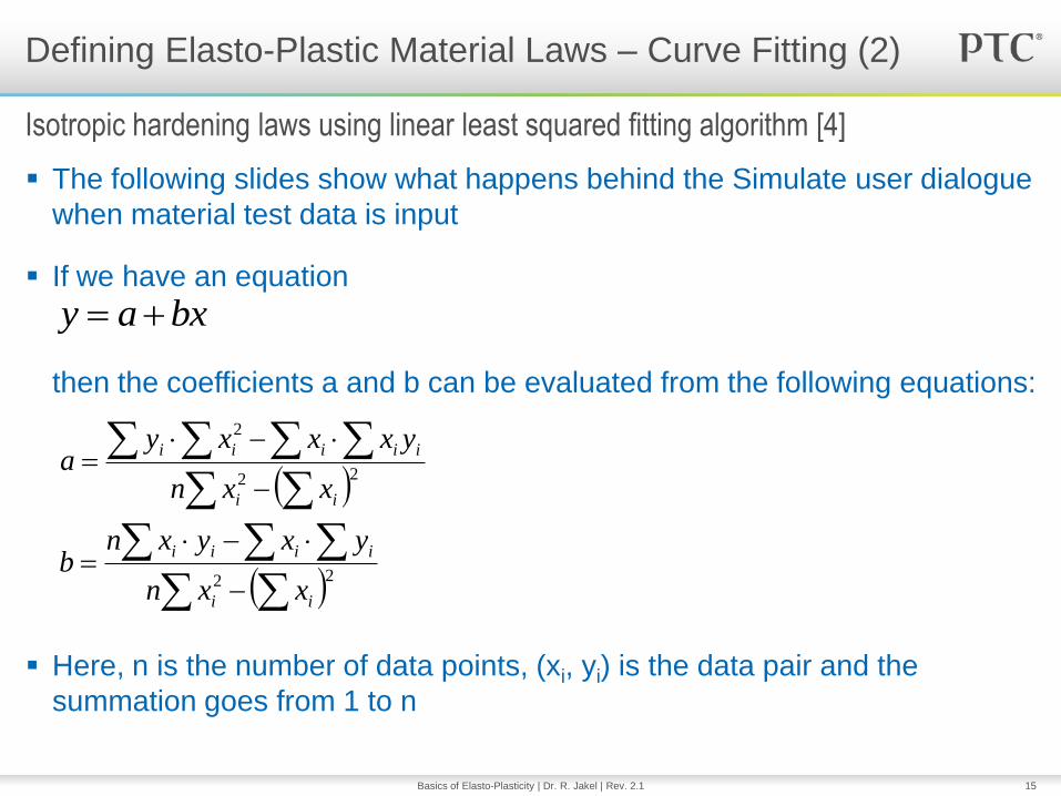
The following slides show what happens behind the Simulate user dialogue
when material test data is input
If we have an equation
then the coefficients a and b can be evaluated from the following equations:
Here, n is the number of data points, (xi, yi) is the data pair and the
summation goes from 1 to n
Defining Elasto-Plastic Material Laws – Curve Fitting (2)
Isotropic hardening laws using linear least squared fitting algorithm [4]
Basics of Elasto-Plasticity | Dr. R. Jakel | Rev. 2.1
bxay
22
22
2
ii
iiii
ii
iiiii
xxn
yxyxnb
xxn
yxxxya

16
Linear plasticity
or:
Here:
Defining Elasto-Plastic Material Laws – Curve Fitting (3)
Application of linear least squared fitting algorithm to isotropic hardening laws [4]
Basics of Elasto-Plasticity | Dr. R. Jakel | Rev. 2.1
BXAY
BXAY
E pmy
Xx
Bb
a
AYy
0

17
Power (potential) plasticity law
or:
Taking logs on either side to the base e:
Here:
Defining Elasto-Plastic Material Laws – Curve Fitting (4)
Application of linear least squared fitting algorithm to isotropic hardening laws (cont‟d)
Basics of Elasto-Plasticity | Dr. R. Jakel | Rev. 2.1
m
m
pmy
BXAY
E
XmBAY eee logloglog
Xx
mb
Ba
AYy
e
e
e
log
log
log

18
Exponential plasticity law
or:
Taking derivatives on either side, with respect to X:
Taking logs on either side to the base e:
Defining Elasto-Plastic Material Laws – Curve Fitting (5)
Application of linear least squared fitting algorithm to isotropic hardening laws (cont‟d)
Basics of Elasto-Plasticity | Dr. R. Jakel | Rev. 2.1
mX
py
BeBAY
mXBAY
m
exp1
exp1lim
mXmBedX
AYd
mXmB
dX
AYdee
loglog

19
Then, we obtain:
After evaluating m (from b),
we can evaluate B (from a)
Defining Elasto-Plastic Material Laws – Curve Fitting (6)
Application of linear least squared fitting algorithm to isotropic hardening laws (cont‟d)
Basics of Elasto-Plasticity | Dr. R. Jakel | Rev. 2.1
Xx
mb
mBa
dX
AYdy
e
e
log
log

20
The material laws are a one dimensional relation of stress versus plastic
strain. Only uniaxially tension loaded specimens are used for characterizing
the elasto-plastic material behavior, where we have one yield point only.
In the three-dimensional space of the principal stresses (σ1, σ2, σ3), an
infinite number of yield points form together the yield surface.
In real structures, we usually have biaxial stress states at the surface and
– more or less – three-axial stress states within the structure. Hence, we
need a suitable criteria to form an equivalent uniaxial, scalar comparative
stress, called the yielding condition or yield criteria.
In literature, several different yield criteria can be found for isotropic
materials.
The subsequent slide shows only the most popular criteria for yielding of
isotropic, ductile materials.
Multi-Axial Plasticity (1)
Yield point and yield surfaces
Basics of Elasto-Plasticity | Dr. R. Jakel | Rev. 2.1

21
Maximum Shear Stress Theory (Tresca yield criterion) – Yield in ductile materials is usually caused by the slippage of crystal planes along the maximum
shear stress surface.
– The French scientist Henri Tresca assumed that yield occurs when the shear stress exceeds the
uniaxial shear yield strength ys:
Distortion Energy Theory (von Mises yield criterion) – This theory proposes that the total strain energy can be separated into two components: the
volumetric (hydrostatic) strain energy and the shape (distortion or shear) strain energy. It is
assumed that yield occurs when the distortion component exceeds that at the yield point for a
simple tensile test. The hydrostatic strain energy is ignored.
– Based on a different theoretical derivation it is also referred to as “octahedral shear stress theory”
– Simulate supports this yield criteria only, since it is most commonly used and often fits with
experimental data of very ductile material
Multi-Axial Plasticity (2)
Classical isotropic yield criteria
Basics of Elasto-Plasticity | Dr. R. Jakel | Rev. 2.1
ys
2
31max
22
13
2
32
2
212
1y

22
In the three-dimensional space of
the principal stresses (σ1, σ2, σ3), an
infinite number of yield points form
together the yield surface. If the
stress state is within this surface, no
yielding appears.
The most popular criteria, Tresca
and von Mises,
look like shown right
The von Mises yield surface is
therefore called the “yield cylinder”
Multi-Axial Plasticity (3)
Graphical representation of classical criteria
Basics of Elasto-Plasticity | Dr. R. Jakel | Rev. 2.1
22
13
2
32
2
212
1y
ys
2
31max
- von Mises - Tresca (max. shear)
1 y -y
y
-y
2
Yield criteria for plane stress (3=0, top)
and any three-axial stress state (bottom)
1
y
-y
y
-y
2
3
-y
2D
3D
yielding
no yielding
y

23
Generalized Isotropic Yield Criterion (Hosford)
– Experimental and theoretical data on yielding under combined stresses can be described by a
single parameter, n, with 1 ≤ n ≤
– For n=2, this equals the von Mises criterion
– This criterion was proposed in 1972 by W. F. Hosford, Department of Materials and Metallurgical
Engineering, The University of Michigan, Ann Arbor, Mich [7]
More criteria and deeper information can be found e.g. in [8] and [9]
Multi-Axial Plasticity (4)
Other Isotropic yield criteria
Basics of Elasto-Plasticity | Dr. R. Jakel | Rev. 2.1
y
nnnn
/1
133221
2
24
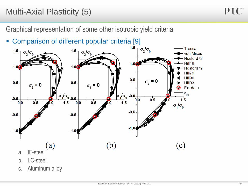
Comparison of different popular criteria [9]
a. IF-steel
b. LC-steel
c. Aluminum alloy
Multi-Axial Plasticity (5)
Graphical representation of some other isotropic yield criteria
Basics of Elasto-Plasticity | Dr. R. Jakel | Rev. 2.1

25
Note the von Mises yielding condition must always be satisfied:
This has some consequences, e.g.: – In a uniaxial stress state, the yield stress and the maximum principal stress will always be the
same – the maximum principal stress can never by greater than the von Mises stress!
– In a biaxial stress state, it may happen that one or more principal stresses may well be above or
below the uniaxial yield stress, so do not be surprised!
– In equi-triaxial tension, yielding will never appear, since the principal stress differences are zero.
The material will break if the principal stress reaches ultimate stress, while the von Mises stress
will still be zero. A ductile material will behave brittle in this case, that means rupture appears
suddenly without previous yielding!
In the following slides, we will examine some characteristic stress states
with a small demonstration model for better understanding
Examination of Typical Stress States (1)
Von Mises Stress and Principal Stresses
Basics of Elasto-Plasticity | Dr. R. Jakel | Rev. 2.1
213
2
32
2
21
22 yield
26
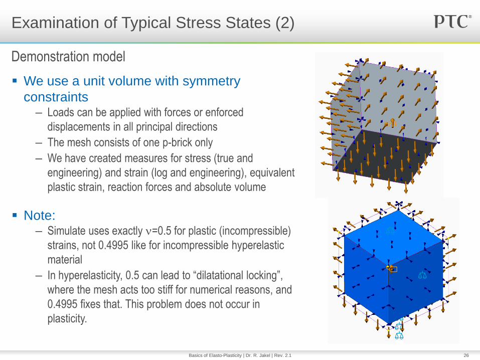
We use a unit volume with symmetry
constraints – Loads can be applied with forces or enforced
displacements in all principal directions
– The mesh consists of one p-brick only
– We have created measures for stress (true and
engineering) and strain (log and engineering), equivalent
plastic strain, reaction forces and absolute volume
Note: – Simulate uses exactly =0.5 for plastic (incompressible)
strains, not 0.4995 like for incompressible hyperelastic
material
– In hyperelasticity, 0.5 can lead to “dilatational locking”,
where the mesh acts too stiff for numerical reasons, and
0.4995 fixes that. This problem does not occur in
plasticity.
Examination of Typical Stress States (2)
Demonstration model
Basics of Elasto-Plasticity | Dr. R. Jakel | Rev. 2.1

27
Simple linear hardening and perfect plasticity
model used – Very soft model steel with
• E=200000 MPa
• Yield strength = 100 MPa
• Elastic Poisson ratio = 0.3
• Tangent modulus (linear hardening only) = 2000 MPa
– At its yield strength, the strain should be
– The lateral strains are:
– At the yield strength, the unit volume of V0=1 mm3
increases to
– All subsequent analyses performed in LDA
Examination of Typical Stress States (3)
Material model used
Basics of Elasto-Plasticity | Dr. R. Jakel | Rev. 2.1
%05.00005.01
11 E
%015.000015.0132
E
2
3211 0002.1)1)(1)(1( mmV Note:
Log strain LDA results are translated into
engineering strains with computed
measures, e.g.

28
Perfect plasticity results – Axial stress stays constant at 100 MPa after yielding
– Volume does not further increase when material yields, like expected
Examination of Typical Stress States (4)
Uniaxial Tension
Basics of Elasto-Plasticity | Dr. R. Jakel | Rev. 2.1
1 y -y
y
-y
2

29
Linear hardening results – Axial stress = 1st principal stress increases with factor 100 reduced slope after yielding
– Volume further increases when material yields: Elastic strain increases because stress
increases during yielding, too! (Note: Analysis was performed in LDA, since SDA cannot
capture this volume change very accurately)
Examination of Typical Stress States (5)
Uniaxial Tension
Basics of Elasto-Plasticity | Dr. R. Jakel | Rev. 2.1

30
We load the volume with the uniaxial yield limit
strength: – Von Mises stress vs. equivalent plastic strain reflects the
uniaxial linear hardening material input curve, like expected
Examination of Typical Stress States (6)
Pure Torque (1)
Basics of Elasto-Plasticity | Dr. R. Jakel | Rev. 2.1
0Yyx 1 y -y
y
-y
2

31
– The max. and min. principal stresses (= x and y-stress)
show yielding much below the uniaxial yield strength of
100 MPa!
Examination of Typical Stress States (7)
Pure Torque (2)
Basics of Elasto-Plasticity | Dr. R. Jakel | Rev. 2.1

32
– The volume should not change for this loading state, just
small numerical disturbances
– Strain energy increases dramatically after von Mises stress
reaches yield limit of 100 MPa
Examination of Typical Stress States (8)
Pure Torque (3)
Basics of Elasto-Plasticity | Dr. R. Jakel | Rev. 2.1

33
– This biaxial, plane stress state allows to load the material
well above the uniaxial yield limit without yielding!
– Just above 1 = x = 115 MPa yielding takes place,
15 % above the unixial limit
Examination of Typical Stress States (9)
Biaxial tension ratio: 1 = 1.2 Y0; 2 = 0.5 Y0; 3=0
Basics of Elasto-Plasticity | Dr. R. Jakel | Rev. 2.1
1 y -y
y
-y
2

34
– The graph Y-Stress vs. Y-strain shows a sharp bend, since
negative incompressible Y-strain prevails after yielding!
– The von Mises stress vs. X-strain shows the uniaxial
material behavior, like expected
Examination of Typical Stress States (10)
Biaxial tension ratio: 1 = 1.2 Y0; 2 = 0.5 Y0; 3=0
Basics of Elasto-Plasticity | Dr. R. Jakel | Rev. 2.1

35
We load all directions, e.g. – Yielding never appears, since all principal stress differences are zero
– In equitriaxial tension, the ductile material will suddenly break brittle
when ultimate strength is reached, without previous yielding
– Under hydrostatic pressure, yielding or even rupture in general will not
appear under practical achievable pressures
Examination of Typical Stress States (11)
Equitriaxial tension
Basics of Elasto-Plasticity | Dr. R. Jakel | Rev. 2.1
010Yzyx
1
y
-y
y
-y
2
3
-y
y

36
Bauschinger effect – If a metallic material is loaded above its yield strength and
the load is reversed, its yield strength in the reversed
direction becomes reduced
– This effect was described by Johann Bauschinger
(1834-1893, Prof. for engineering mechanics at the
Munich Polytechnikum)
– The analogous model for this effect is shown right below:
It consists of a spring K1 representing the elastic material
behavior. In serial connection to K1 , there is a friction
element FR and another spring K2 (usually K2 << K1) in
parallel connection
Hardening Models (1)
Basics of material hardening
Basics of Elasto-Plasticity | Dr. R. Jakel | Rev. 2.1
yy y
y
K2
K1
FR
37
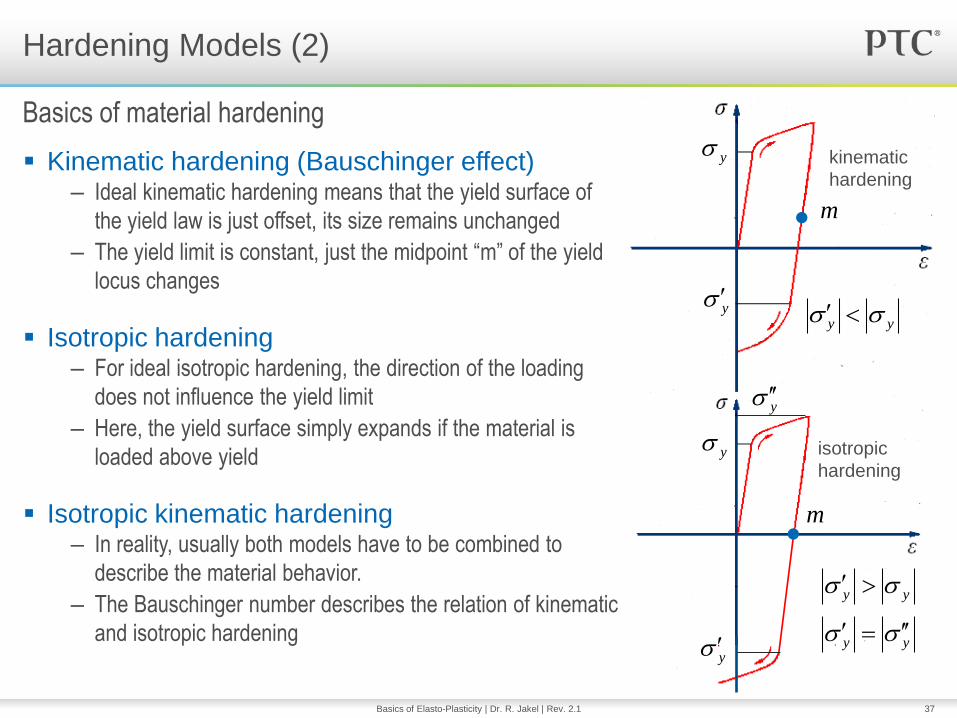
Kinematic hardening (Bauschinger effect) – Ideal kinematic hardening means that the yield surface of
the yield law is just offset, its size remains unchanged
– The yield limit is constant, just the midpoint “m” of the yield
locus changes
Isotropic hardening – For ideal isotropic hardening, the direction of the loading
does not influence the yield limit
– Here, the yield surface simply expands if the material is
loaded above yield
Isotropic kinematic hardening – In reality, usually both models have to be combined to
describe the material behavior.
– The Bauschinger number describes the relation of kinematic
and isotropic hardening
Hardening Models (2)
Basics of material hardening
Basics of Elasto-Plasticity | Dr. R. Jakel | Rev. 2.1
yy y
y
yy
yy
y
y
y
m
kinematic
hardening
isotropic
hardening
m
38
Opportunities & Limitations
Tips & Tricks
Applying Simulate to Elasto-Plastic Problems
Basics of Elasto-Plasticity | Dr. R. Jakel | Rev. 2.1
Part II

39
Isotropic hardening – Creo Simulate supports isotropic
hardening only, therefore currently the
Bauschinger effect cannot be described
Example – Simple linear hardening material used
Load history:
Isotropic Hardening (1)
Application in Creo Simulate (1)
Basics of Elasto-Plasticity | Dr. R. Jakel | Rev. 2.1
t

40
Cyclic Loading – Since currently only isotropic hardening is supported,
cyclic loading especially with the linear hardening or
Power law is not realistic, because the material will
“harden until infinity”.
Preferred Material Model – In this case, approximate with perfect plasticity or
exponential hardening law (both have an upper limit).
Load history
Isotropic Hardening (2)
Application in Creo Simulate (2)
Basics of Elasto-Plasticity | Dr. R. Jakel | Rev. 2.1
t

41
Plastic material laws and test data – When entering the elasto-plastic material/test data into the data dialogue, note that you have to
enter engineering stress vs. engineering plastic strain for SDA and true stress vs. logarithmic
plastic strain for LDA. Subtract the elastic strain from the total strain to get the plastic strain
required for input. Note the curves start with the yield limit stress, not at zero!
– For all material laws except of perfect plasticity, the entered stress must be a strictly monotonic
function of the engineering strain. A decrease of engineering stress at higher strains cannot be
described in a SDA (see example 1 of part III for further details).
– Only the exponential plasticity law allows to define an upper limit of plastic stress, which is
approached asymptotic!
– The material laws do not allow to calculate (accidently) necking under high loads in the plastic
domain, if there is no imperfection in the model; so they do not allow to predict where failure will
really appear (see again example 1 of part III for further details).
Stress and strain output – Note that Simulate will output engineering stress and strain in plasticity only if “calculate large
displacements” (=LDA) is not activated. If an LDA is performed, since Creo 1.0 Simulate outputs
logarithmic strain and true stress (until Wildfire 5, output is Almansi (Eulerian) strain).
Working with Material Laws in Simulate (1)
What do I have to take care about when I use a material law within Simulate?
Basics of Elasto-Plasticity | Dr. R. Jakel | Rev. 2.1

42
Working with Material Laws in Simulate (2)
Graphical representation of different strains [2]:
Basics of Elasto-Plasticity | Dr. R. Jakel | Rev. 2.1
10
01
l
ll
ln/ln 01 llL
2
0
2
0
2
1
2
1
l
llG
2
1
2
0
2
1
2
1
l
llE
stretch =l1/l0
str
ain
Reported since Creo Simulate in LDA: Logarithmic strain
(also called “natural”, “true”, or “Hencky” strain),
obtained by integrating the incremental strain:
Reported until Wildfire 5 in LDA: Almansi Strain
...432
)1ln(
lnln
432
0
1
11
1
0
L
L
l
lLL
l
l
l
l
l
l

43
Literature separates between “small strain”
and “finite strain” plasticity – In small strain plasticity, just small deformations are
allowed and the total deformations as well as the
deformation increments are additively split into an
elastic and plastic part, = e+p. This assumption is
valid for strains up to a few percent, then it becomes
inaccurate
– In finite strain plasticity theory, the deformation
gradient is split multiplicatively into an elastic and a
plastic part. This allows to treat problems with very
large deformations, like forging processes.
– The mathematical methods especially of finite strain
plasticity are very ambitious and far beyond the
scope of this presentation.
Small Strain and Finite Strain Plasticity (1)
Small and finite strain plasticity
Basics of Elasto-Plasticity | Dr. R. Jakel | Rev. 2.1

44
Creo Elements / Pro Mechanica WF 5.0 supports small strain plasticity – Here, the relation between total strain and displacement is linear: Strains are output as
engineering values.
– Plasticity is limited to SDA (small displacement analysis) only, LDA (large displacement
analysis) therefore is not supported in this release
Creo Simulate 1.0 and 2.0 also support finite strain plasticity: – Finite strain is implemented for 3D models if LDA is activated.
– In this case, the plastic (and elastic) strain is output as logarithmic strain: Simulate computes
incremental strain at each load step and then integrates it to get total strain. This ends up with
strain being logarithmic (see slide 42).
– For 2D models (plane stress, strain & axial symmetric), still just small strain plasticity is
supported. So if LDA is used with these model types even though, e.g. in combination with a
contact analysis, hyperelastic material, or nonlinear spring, Simulate issues a warning if the
strain becomes > 10 %
– Internally, the engine still uses large displacement calculations in this case, but the strain
calculations in the 2D elasto-plastic elements themselves are small strain.
Small Strain and Finite Strain Plasticity (2)
Mechanica WF 5.0 and Creo Simulate differ in plasticity models
Basics of Elasto-Plasticity | Dr. R. Jakel | Rev. 2.1

45
What can I do if a need finite strain calculations, but have a 2D problem? – In these cases (plane stress, plane strain or axial symmetric models), built up your model as
3D segment with a small angle or thin slice using appropriate constraints and mesh controls
– Example: An axial symmetric problem as 2D axial symmetric and as 3D segment model:
– Plane strain models can be set up by using just one layer of elements over the constant “slice”
thickness and use mirror symmetry constraints at the slice cutting surfaces, see [10].
Small Strain and Finite Strain Plasticity (3)
Performing finite strain analyses
Basics of Elasto-Plasticity | Dr. R. Jakel | Rev. 2.1

46
How is the “equivalent plastic strain” being computed? – The computation uses the following variables:
“effectiveStressPredictor”: current von Mises Stress
“flowStress”: yield stress based on current plastic strain and strain-hardening curve
“ShearModulus”: elastic shear modulus = E/(2*(1+nu)) where nu is the elastic Poisson’s ratio
“dep”: incrememental equivalent plastic strain
“dStress”: the slope of the work hardening curve
– At each load increment, the incremental plastic strain “dep” is given by:
dep = 0
Loop until ddep stops changing:
{
yieldFunction = effectiveStressPredictor - flowStress - 3.0*ShearModulus*dep
denominator = 3.0*ShearModulus + dStress;
ddep = yieldFunction/denominator;
dep = dep +ddep;
}
– After this loop, the equivalent plastic strain “ep”, is incremented by “dep”. Note ep is logarithmic
strain, like all strain quantities in LDA since Creo Simulate 1.0.
Characteristic Measures in Plasticity (1)
Equivalent plastic strain
Basics of Elasto-Plasticity | Dr. R. Jakel | Rev. 2.1

47
Von Mises Stress – Von Mises stress is derived under the assumption that
distortion energy of any arbitrary loading state drives
the damage of the material:
– Per definition, in an uniaxial tension test case with just
1 >0 and 2 = 3 =0 we obtain for the von Mises
Stress:
Characteristic Measures in Plasticity (2)
Von Mises Stress and Strain
Basics of Elasto-Plasticity | Dr. R. Jakel | Rev. 2.1
2
13
2
32
2
212
1 vM
1
2
1
2
12
1 vM

48
Von Mises Strain in Simulate – Simulate currently uses this equation for von Mises
Strain:
– This equation is used in formal analogy to the von
Mises stress only for computational reasons (same
subroutine as for stress) and simplicity.
– This strain will be analyzed on demand as measure
output only for certain locations or over certain
references. It is calculated at the end only and not used
for any other result output.
– Note that this von Mises strain definition cannot be
used directly for comparison with the longitudinal strain
in an uniaxial test. It must be modified, e.g. with help of
a computed measure, like shown in the subsequent
slides.
Characteristic Measures in Plasticity (3)
Von Mises Stress and Strain
Basics of Elasto-Plasticity | Dr. R. Jakel | Rev. 2.1
2
13
2
32
2
212
1 vM

49
Von Mises Strain – In analogy to the von Mises stress, for comparing any three dimensional loading state with the
state of uniaxial loading the von Mises strain definition in Simulate must be corrected: An
additional factor 1/(1+´) should be taken into account, like e.g. used in [5]:
– Herein, ‟ is the effective Poisson‟s ratio, which is 0.5 for plastic strains (incompressible) or the
material Poisson‟s ratio for elastic and thermal strains
– The following slides show that this equation reflects a scalar comparative strain for comparison
with the longitudinal strain in a uniaxial test
Difficulties in von Mises strain correction – If the loading state of the material is just in the elastic domain, this correction can be easily
applied, since the elastic Poisson‟s ratio is known
– If the loading state is far in the plastic domain, the elastic deformation can be neglected and ´
becomes 0.5
– The problem is the domain with small plastic deformations, since here it is not known which
strain type prevails, so which fraction of the deformation is plastic and which is elastic
Characteristic Measures in Plasticity (4)
Von Mises Strain modification
Basics of Elasto-Plasticity | Dr. R. Jakel | Rev. 2.1
2
13
2
32
2
212
1
1
1
vM

50
Hooke’s law – Hooke„s law for isotropic material expressed in principal stresses and strains:
– In an uniaxial tensile test, we have just one positive principal stress 1,
resulting in a three-dimensional strain state:
– The von Mises comparative strain equation should deliver the same strain like the axial strain 1
Characteristic Measures in Plasticity (5)
Von Mises Strain definition in the uniaxial case
Basics of Elasto-Plasticity | Dr. R. Jakel | Rev. 2.1
2133
3122
3211
1
1
1
E
E
E
132
11
32
1
1
0
/
E
E
AF

51
Von Mises Strain – Let‟s examine if the corrected von Mises Strain definition works correct for uniaxial loading,
where we have:
– Putting this into the von Mises Strain equation, we obtain with = ‟ :
– So, per definition now the von Mises Strain equation delivers the uniaxial tensile strain 1 for the
uniaxial loading state
Characteristic Measures in Plasticity (6)
Von Mises Strain definition in the uniaxial case
Basics of Elasto-Plasticity | Dr. R. Jakel | Rev. 2.1
13211
321
;1
0;/
EE
AF
...1
11
111
1
10
12
2
1
1
1
11
2
1
1
1
11
111
2
2
11
2
11
2
11
2
11
deqE
EE
v
EE
v
E
EE
v
E
v
E
v
E
v
E
vM
vM
vM

52
Loading – Creo Simulate offers a powerful time history functionality
using “dummy time” steps.
– Load stepping is available in two ways:
• The user can use default or self-defined functions, e.g. as
tabular values. In this case, output steps should be kept
“automatic”, then for all tabular time values a result will be
computed
• Output steps can also be set to “User defined”, with automatic
or manual time stepping.
– Simulate has a built-in automatic load step refinement in
case of too big increments, but this should not be
overstressed!
– A good user load
stepping can
significantly increase
performance!
Load Stepping and Unloading (1)
What do I have to take care about if I want to load my structure?
Basics of Elasto-Plasticity | Dr. R. Jakel | Rev. 2.1

53
Unloading – Unloading can be achieved by simply activating the button
“include unloading”.
– Alternatively, since Creo 1 unloading can be achieved by
using the new load history function just described.
– In addition, Creo 2.0 offers an engine command line option
for advanced users called “lda_gradual_unloading”
(unsupported for testing by advanced users only). This
assures that unloading with the button “include unloading”
is done not in one single, but a series of 10 consecutive
steps.
– The reason for this command line option is that unloading
the structure in one single step may lead in some cases to
inaccurate results. Usually, this can be clearly detected by
checking the von Mises stress distribution: It will look noisy,
having many randomly located “hot spots” that are
obviously not reasonable.
Load Stepping and Unloading (2)
What do I have to take care about if I want to unload my structure?
Basics of Elasto-Plasticity | Dr. R. Jakel | Rev. 2.1

54
Mesh controls – A good mesh in a nonlinear material analysis is much more
important than in a linear analysis, because it helps the analysis
to run faster or more accurate within the same time.
– Especially problems with very large strains take benefit of a
smooth, undistorted mesh with bricks and wedges instead of tets.
– The new mesh controls for regular meshing should therefore be
used whenever possible.
Meshing
When using elasto-plastic materials, what do I have to take care regarding meshing?
Basics of Elasto-Plasticity | Dr. R. Jakel | Rev. 2.1

55
Application Examples
Basics of Elasto-Plasticity | Dr. R. Jakel | Rev. 2.1
Part III

56
Goals of the study: – Understand why a uniaxial tension test specimen made of
ductile material breaks in the necked area under 45° at the
outer surface and brittle in its center (see slide 7 or [3])
– Understand differences of SDA and LDA in plasticity
– Understand the influence of necking in the true and
engineering stress-strain curves
Remark: – The material laws in Simulate do not directly allow to
simulate necking in a perfect specimen with regular mesh,
which appears in reality at an accidental weak location of
the tensile test specimen.
– Therefore, we use a second cylindrical specimen in the
LDA with a small imperfection modeled into the geometry
like shown right: The cylinder radius is just locally 5/100 mm
smaller than the nominal radius of 10 mm
– We will analyze the perfect specimen in both SDA and LDA
A Uniaxial Test Specimen with Necking (1)
Study of a tensile test specimen with taking into account necking
Basics of Elasto-Plasticity | Dr. R. Jakel | Rev. 2.1

57
Model setup: – We use mapped meshing for the
90° symmetry section to obtain a
regular mesh just using bricks (and
wedges only at the rotation axis).
– From the reaction forces at the
constraints, we analyze nominal
engineering and true stress in the
necked section with help of
computed measures.
– Engineering strain (not output in
LDA) is computed by the specimen
elongation divided by its initial
length (computed measure).
– We use an enforced displacement
to apply the load, for better
numerical stability in the region of
high plastic strains.
A Uniaxial Test Specimen with Necking (2)
Study of a tensile test specimen with taking into account necking
Basics of Elasto-Plasticity | Dr. R. Jakel | Rev. 2.1
58
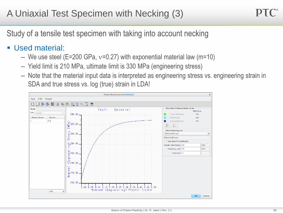
Used material: – We use steel (E=200 GPa, =0.27) with exponential material law (m=10)
– Yield limit is 210 MPa, ultimate limit is 330 MPa (engineering stress)
– Note that the material input data is interpreted as engineering stress vs. engineering strain in
SDA and true stress vs. log (true) strain in LDA!
A Uniaxial Test Specimen with Necking (3)
Study of a tensile test specimen with taking into account necking
Basics of Elasto-Plasticity | Dr. R. Jakel | Rev. 2.1
59
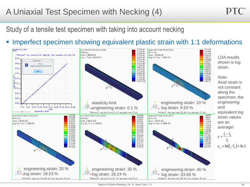
Imperfect specimen showing equivalent plastic strain with 1:1 deformations
A Uniaxial Test Specimen with Necking (4)
Study of a tensile test specimen with taking into account necking
Basics of Elasto-Plasticity | Dr. R. Jakel | Rev. 2.1
elasticity limit
engineering strain: 0.1 %
engineering strain: 10 %
log strain: 9.53 %
engineering strain: 20 %
log strain: 18.23 % engineering strain: 30 %
log strain: 26.24 % engineering strain: 40 %
log strain: 33.65 %
LDA results,
shown is log
strain.
Note:
Axial strain is
not constant
along the
specimen, the
engineering
and
equivalent log
strain values
are an
average!
ln/ln 01
0
01
ll
l
ll
L

60
Equivalent plastic strain and von Mises stress results animations
A Uniaxial Test Specimen with Necking (5)
Study of a tensile test specimen with taking into account necking
Basics of Elasto-Plasticity | Dr. R. Jakel | Rev. 2.1

61
Principal stress vector results at
max. engineering strain in the
necked cross section center – In the center of the necked region, a
triaxial tensile stress state appears
– In our example, the three principal
stresses are not the same like stated in
[3], but in the specimen center radial
and circumferential stress have similar
size and are approximately 60 % of the
axial principal stress
– Triaxial tension leads to brittle rupture in
the specimen, whereas at the specimen
surface we just have a two-axial stress
state (radial stress=0): There, we have
ductile behavior.
A Uniaxial Test Specimen with Necking (6)
Study of a tensile test specimen with taking into account necking
Basics of Elasto-Plasticity | Dr. R. Jakel | Rev. 2.1
Triaxial tension
(Quick check results only)!
1 = ax 886 Mpa
2 = 3 546 Mpa

62
True and engineering stress vs. engineering strain in SDA and LDA
A Uniaxial Test Specimen with Necking (7)
Study of a tensile test specimen with taking into account necking
Basics of Elasto-Plasticity | Dr. R. Jakel | Rev. 2.1
elongation without necking necking becomes visible necking
starts
Inflection point of true stress-
strain curve: Necking starts!
Due to SDA theory simplifications,
the volume change (lateral con-
traction) is overestimated, and the
true stress becomes too high at
strains >10%
Note for shown curves:
1) Eng strain is calculated
by specimen elongation
l / initial length l
2) True stress in the
imperfect specimen is an
average value and
analyzed by reaction
force / actual necked
cross section area
3) Engineering stress in the
imperfect specimen is
analyzed by reaction
force / initial cross
section area
4) The material input curve
for true stress vs. log
strain -translated to eng
strain- is not shown, but
virtually the same like the
shown green stress vs.
eng. strain curve

63
Conclusions: – The subtraction of elastic strain from the measured curve is just a small correction.
– Note that you may need different material data sets for SDA and LDA.
– For small strains, it is sufficient to measure engineering stress vs. engineering strain and run
an SDA analysis.
– For bigger strains, e.g. 5% and more, true stress vs. true strain should be input into the
material dialogue. Run an LDA analysis in this case! This is especially important if you want to
do a metal forming analysis, where strains may rapidly become 30% and more.
– True stress results from specimens in the necked region should not be taken into account,
since they will falsify the material data curve. Take care that you input data just from the strain
region without necking (true stress curve has an inflection point when necking starts)!
– When necking appears, the axial strain along the specimen length is not constant any longer
(see the animations on slide 60). A further increase of strain will just take place in the necked
area.
– As a result check, you may run an analysis with your tensile test specimen and compare
material data input curve and analysis result like shown in the example.
A Uniaxial Test Specimen with Necking (8)
Study of a tensile test specimen with taking into account necking
Basics of Elasto-Plasticity | Dr. R. Jakel | Rev. 2.1

64
Useful equations for uniaxial test data evaluation: – For translating stress data:
– For translating strain data:
Summary of required stress/strain input in Simulate:
A Uniaxial Test Specimen with Necking (9)
Study of a tensile test specimen with taking into account necking
Basics of Elasto-Plasticity | Dr. R. Jakel | Rev. 2.1
Material SDA/LDA Stress Strain
hyperelastic LDA (no hyperelasticity support in SDA)
nominal (engineering) nominal (engineering)
elastoplastic SDA (small strain) nominal (engineering) nominal (engineering)
elastoplastic LDA (finite strain) true true (logarithmic)
E
E
e
trueengpl
eng
engpleng
eng
eng
trueeng
engengtrue
)1ln(
1
)1ln(
)exp(/
)1(
ln,
,
ln
ln
ln

65
Geometry: – Two ideal-elastic plates compress a soft Aluminum
tube (displacement controlled)
– Half symmetry model to increase speed
Material: – Power law used for elasto-plastic description
Flattening of a Tube End (1)
Model setup
Basics of Elasto-Plasticity | Dr. R. Jakel | Rev. 2.1

66
Flattening of a Tube End (2)
Displacement results animation (quick check only)
Basics of Elasto-Plasticity | Dr. R. Jakel | Rev. 2.1
deformed shape

67
Flattening of a Tube End (3)
Von Mises stress results animation (quick check only)
Basics of Elasto-Plasticity | Dr. R. Jakel | Rev. 2.1
deformed shape with
released forming plates

68
Geometry: – A thin flat steel disk is formed to become a
membrane
– The steel disk is guided at the outer diameter with
help of a ring
– The displacement controlled grey piston forms the
wave
Model: – For simplicity, the 2D axial symmetric model
formulation is used.
– Note this is just a coarse approximation since we
expect log strains of >30 % and small strain
plasticity is not accurate here. An alternative,
better suitable 3D segment model supporting
finite strain is shown on slide 45.
– LDA is used for better contact modeling, since we
have large deformations at the contacts.
Forming of a Thin Membrane (1)
Model setup
Basics of Elasto-Plasticity | Dr. R. Jakel | Rev. 2.1
69
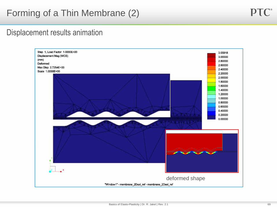
Forming of a Thin Membrane (2)
Displacement results animation
Basics of Elasto-Plasticity | Dr. R. Jakel | Rev. 2.1
deformed shape

70
Forming of a Thin Membrane (3)
Equivalent plastic strain results animation
Basics of Elasto-Plasticity | Dr. R. Jakel | Rev. 2.1
deformed shape with
released piston

71
Questions?
Thanks for your attention!
Basics of Elasto-Plasticity | Dr. R. Jakel | Rev. 2.1

72
Literature
Technical Dictionary English-German
Appendix
Basics of Elasto-Plasticity | Dr. R. Jakel | Rev. 2.1
Part IV

73
[1] Wikipedia: Yield (engineering)
http://en.wikipedia.org/wiki/Yield_(engineering)
[2] R. Jakel: Analysis of Hyperelastic Materials with MECHANICA
– Theory and Application Examples –
Presentation for the 2nd SAXSIM | Technische Universität Chemnitz
27. April 2010 | Rev. 1.1
[3] W. Domke: Werkstoffkunde und Werkstoffprüfung, 9. Auflage 1981, Verlag
W. Giradet, Essen, ISBN 3-7736-1219-2
[4] John Yang, PTC Mechanica R&D: Handwritten Notes
[5] ANSYS Release 11.0 user documentation,
chapter 2.4. Combined Stresses and Strains,
http://www.kxcad.net/ansys/ANSYS/ansyshelp/thy_str4.html
Literature Sources (1)
Basics of Elasto-Plasticity | Dr. R. Jakel | Rev. 2.1

74
[6] Gordon R. Johnson, William H. Cook: A constitutive model and data for
metals subjected to large strains, high strain rates and high temperatures;
Work funded by Contract F08635-81-C-0179 from the U.S. Air Force and
a Honeywell Independent Development Program, 1983
[7] W.F. Hosford, A Generalized Isotropic Yield Criterion, J. Appl. Mech.,
June 1972, Volume 39, Issue 2, 607
http://dx.doi.org/10.1115/1.3422732
[8] Richard M. Christensen, Prof. Research Emeritus, Aeronautics and
Astronautics Dept., Stanford University, http://www.failurecriteria.com
[9] Yanshan Lou, Hoon Huh: Yield loci evaluation of some famous yield
criteria with experimental data, KSAE09-J0003, 2009
[10] R. Jakel: Pro/ENGINEER Mechanica Wildfire 4.0, Workshop
Fundamentals II, p. 15 ff, Rev. 2.0.1, 2011 (PTC CER workshop material)
Literature Sources (2)
Basics of Elasto-Plasticity | Dr. R. Jakel | Rev. 2.1

75
– dilatation – Dilatation, Ausdehnung
– dislocation: Gitterfehler, Versetzung
– elastic – perfectly plastic material law: ideal elastisch – ideal plastisches Materialgesetz
– elongation without necking: Gleichmaßdehnung
– elongation with necking: Einschnürdehnung
– finite strain plasticity: Theorie der Plastizität großer Deformationen
– gray cast iron: Grauguss
– hardened steel: gehärteter Stahl
– isotropic hardening: Isotrope Verfestigung
– kinematic hardening: Kinematische Verfestigung
– tempered steel: vergüteter Stahl
– proof stress: Dehngrenze, Ersatzstreckgrenze
– soft steel: weicher Stahl
– small strain plasticity: Theorie der Plastizität kleiner Deformationen
– stretch: Streckung ( = l1/l0 = 1+)
– yield limit: Fließgrenze
Technical Dictionary English-German
Used vocabulary in this presentation
Basics of Elasto-Plasticity | Dr. R. Jakel | Rev. 2.1