basics of signals - princeton university

Chapter 2

Basics of Signals

2.1 What are Signals?

As mentioned in Chapter XX, a system designed to perform a particular taskoften uses measurements obtained from the environment and/or inputs from auser. These in turn may be converted into other forms. The physical variablesof interest are generally called signals. In an electrical system, the physicalvariables of interest might be a voltage, current, amount of charge, etc. Ina mechanical system, the variables of interest might be the position, velocity,mass, volume, etc. of various objects. Financial examples might include theprice of a stock, commodity, or option, an interest rate, or an exchange rate.In performing its tasks, the system may need to manipulate or combine varioussignals, extract information, or otherwise process the signals. These actions arecalled signal processing or signal analysis.

A convenient abstraction is to model the value of a physical variable ofinterest by a number. We are usually interested in the physical variable notat just a single time, but rather at a set of times. In this case, the signal is afunction of time, say f(t). For example, f(t) might denote a voltage level, orthe velocity of an object, or the price of a stock at time t.

In some cases, we might be interested in measuring the quantity as a func-tion of some variable other than time. For example, suppose we are interestedin measuring the water temperature in the ocean as a function of depth. In thiscase, the signal is a function of a spatial variable, with f(x) denoting tempera-ture at depth x.

A signal need not be a function of just a single variable. To continue theexample above, suppose we are interested in the temperature at particular pointsin the ocean, not simply as a function of depth. In this case, we might letf(x, y, z) denote the temperature at the point (x, y, z), so the signal is a function

∗ c©1999-2002 by Sanjeev R. Kulkarni. All rights reserved.†Lecture Notes for ELE201 Introduction to Electrical Signals and Systems.‡Thanks to Richard Radke for producing the figures.

1

2 CHAPTER 2. BASICS OF SIGNALS

of three variables. Now, if we are also interested in how the temperature evolvesin time, the signal f(x, y, z, t) would be a function of four variables.

0.05 0.1 0.15 0.2 0.25 0.3 0.35 0.4 0.45 0.5−3

−2

−1

0

1

2

3

seconds

inte

nsity

The word "Matlab"

Figure 2.1: Someone saying the word “Matlab”

Examples of signals that we will encounter frequently are audio signals,images, and video. An audio signal is created by changes in air pressure, andtherefore can be represented by a function of time f(t) with f representingthe air pressure due to the sound at time t. An example of an audio signalof someone saying “Matlab” is shown in Figure 2.1. A black and white imagecan be represented as a function f(x, y) of two variables. Here (x, y) denotes aparticular point on the image, and the value f(x, y) denotes the brightness (orgray level) of the image at that point.

An example of a black and white image is shown in Figure 2.2. A video canbe thought of as a sequence of images. Hence, a black and white video signal canbe represented by a function f(x, y, t) of three variables (two spatial variablesand time). In this case, for a fixed t, f(·, ·, t) represents the still image/frame attime t, while for a fixed (x, y), f(x, y, ·) denotes how the brightness at the point(x, y) changes as a function of time.

Three frames of a video of a commercial are shown in Figure 2.3. It turnsout that color images (or video) can be represented by a combination of threeintensity images (or video, respectively), as will be discussed later in ChapterXX.

2.2 Analog and Digital Signals

Often the domain and the range of a signal f(x) are modeled as continuous.That is, the time (or spatial) coordinate x is allowed to take on arbitrary values(perhaps within some interval) and the value of the signal itself is allowed totake on arbitrary values (again within some interval). Such signals are called

2.2. ANALOG AND DIGITAL SIGNALS 3

Figure 2.2: A gray-scale image.

0:13 0:14 0:15

Figure 2.3: Video frames from a commercial.


analog signals. A continuous model is convenient for some situations, but inother situations it is more convenient to work with digital signals — i.e., signalsthat have a discrete (often finite) domain and range. Two other related wordsthat are often used to describe signals are continuous-time and discrete-time,referring to signals where the independent variable denotes time and takes oneither a continuous or discrete set of values, respectively.

0 2 4 6 8 10 12 14 16 18 2028

29

30

31

32

33

34

35

36

seconds

tem

pera

ture

Sampled version of temperature graph

Figure 2.4: Sampling an analog signal.

Sometimes a signal that starts out as an analog signal needs to be digitized(i.e., converted to a digital signal). The process of digitizing the domain is calledsampling. For example, if f(t) denotes temperature as a function of time, andwe are interested only in the temperature at 1 second intervals, we can samplef at the times of interest as shown in Figure 2.4.

Another example of sampling is shown in Figure 2.5. An original imagef(x, y) is shown together with sampled versions of the image. In the sampledversions of the image, the blocks of constant intensity are called pixels, and thegray level is constant within the pixel. The gray level value is associated withthe intensity at the center of the pixel. But rather than simply showing a smalldot in the center of the pixel, the whole pixel is colored with the same gray levelfor a more natural appearance of the image. The effect of more coarse samplingcan be seen in the various images. Actually, the so-called “original” image inFigure 2.5a is also sampled, but the sampling is fine enough that we don’t noticeany graininess.

The process of digitizing the range is called quantization. In quantizing asignal, the value f(x) is only allowed to take on some discrete set of values (asopposed to the variable x taking on discrete values as in sampling).

Figure 2.6 shows the original temperature signal f(t) (shown previously inFigure 2.4) as well various quantized versions of f . Figure 2.7 shows the imagefrom Figure 2.2 and various quantized versions. In the quantized versions of theimages, the gray levels can take on only some discrete set of values. Actually,


No subsampling 4 x 4 blocks

8 x 8 blocks 16 x 16 blocks

Figure 2.5: Sampling an image.


0 0.5 1 1.5 0

0.2

0.4

0.6

0.8

1 Unquantized signal

0 0.5 1 1.5 0

0.2

0.4

0.6

0.8

1 32 levels

0 0.5 1 1.5 0

0.2

0.4

0.6

0.8

1 16 levels

0 0.5 1 1.5 0

0.2

0.4

0.6

0.8

1 8 levels

Figure 2.6: Quantized versions of an analog signal.

the so-called “original” image is also quantized, but because of the resolutionof the printer and limitations of the human visual system, a technique knownas halftoning (discussed in Chapter XX) can be used so that we don’t noticeany artifacts due to quantization. It is typical in images to let the gray leveltake on 256 integer values with 255 being the brightest gray level and 0 thedarkest. In Figures 2.7d-f there are only 8, 4, and 2 gray levels respectively, andquantization artifacts become quite noticeable.

Sampling and quantization to digitize a signal seem to throw away muchinformation about a signal, and one might wonder why this is ever done. Themain reason is that digital signals are easy to store and process with digitalcomputers. Digital signals also have certain nice properties in terms of robust-ness to noise, as we’ll discuss in Section XX. However, there are also situationsin which analog signals are more appropriate. As a result there is often a needfor analog-to-digital conversion and digital-to-analog conversion (also writtenA/D and D/A conversion). In digitizing signals, one would also like to knowhow much information is lost by sampling and quantization, and how best todo these operations. The theory for sampling is clean and elegant, while thetheory for quantization is more difficult. It turns out that choices for samplingrates and number of quantization levels also depend to a large extent on systemand user requirements. For example, in black-and-white images, 256 gray levelsis adequate for human viewing – much more than 256 would be overkill, whilemuch less would lead to objectionable artifacts. We defer a more detailed con-sideration of sampling and quantization until Chapter XX after we have covered


256 levels

8 levels

32 levels 16 levels

4 levels 2 levels

Figure 2.7: Quantized versions of a gray-scale image.


some additional background material.Before discussing some basic operations on signals, we describe a fairly com-

mon notational convention which we will also follow. Continuous-time signalswill be denoted using parentheses, such as x(t), while discrete-time signals willuse brackets such as x[n]. This convention also applies even if the indepen-dent variable represents something other than time. That is, y(u) denotes asignal where the domain is continuous, while y[k] indicates a discrete domain,whether or not the independent variables u and k refer to time. Often the lettersi, j, k, l,m, n are used to denote a discrete independent variable.

2.3 Some Basic Signal Operations

In addition to the obvious operations of adding or multiplying two signals, anddifferentiating or integrating a signal, certain other simple operations are quitecommon in signal processing. We give a brief description of some of these here.The original signal is denoted by x(t).

−8 −6 −4 −2 0 2 4 6 8

0

2

4

6Original signal, f(x)

−8 −6 −4 −2 0 2 4 6 8

0

2

4

6Amplitude−shifted signal, f(x)+1.5

−8 −6 −4 −2 0 2 4 6 8

0

2

4

6Time−shifted signal, f(x+3)

Figure 2.8: Amplitude- and time-shifted versions of a signal.

The signal a + x(t) where a is some number is just adding a constant signalto x(t) and simply shifts the range (or amplitude) of the signal by the amounta. A somewhat different operation is obtained when one shifts the domain ofthe signal. Namely, the signal x(t− t0) is a time-shift of the original signal x(t)by the amount t0. It’s like a delayed version of the original signal. Figure 2.8shows amplitude and time-shifted versions of a signal.

2.3. SOME BASIC SIGNAL OPERATIONS 9

0 20 40 60 80 100 120 140 160 180 2000

0.1

0.2

0.3

0.4

0.5

0.6

0.7A periodic signal

seconds

Figure 2.9: A periodic signal.

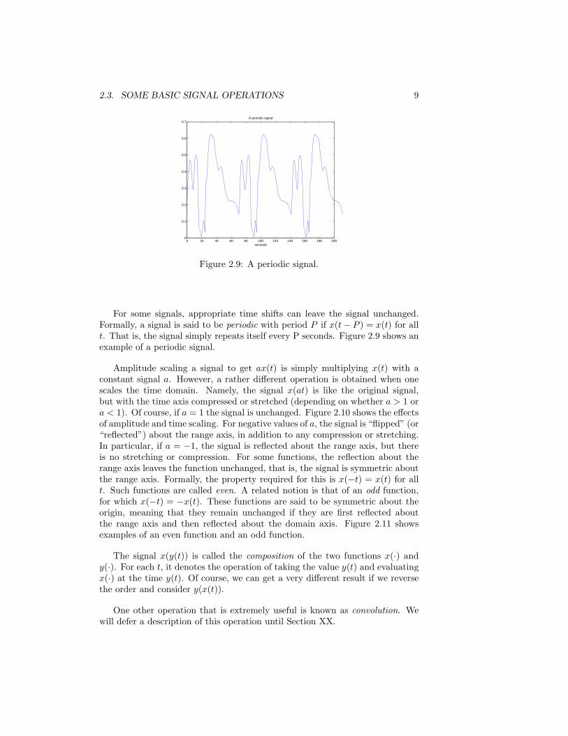
For some signals, appropriate time shifts can leave the signal unchanged.Formally, a signal is said to be periodic with period P if x(t− P ) = x(t) for allt. That is, the signal simply repeats itself every P seconds. Figure 2.9 shows anexample of a periodic signal.

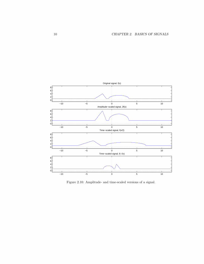
Amplitude scaling a signal to get ax(t) is simply multiplying x(t) with aconstant signal a. However, a rather different operation is obtained when onescales the time domain. Namely, the signal x(at) is like the original signal,but with the time axis compressed or stretched (depending on whether a > 1 ora < 1). Of course, if a = 1 the signal is unchanged. Figure 2.10 shows the effectsof amplitude and time scaling. For negative values of a, the signal is “flipped” (or“reflected”) about the range axis, in addition to any compression or stretching.In particular, if a = −1, the signal is reflected about the range axis, but thereis no stretching or compression. For some functions, the reflection about therange axis leaves the function unchanged, that is, the signal is symmetric aboutthe range axis. Formally, the property required for this is x(−t) = x(t) for allt. Such functions are called even. A related notion is that of an odd function,for which x(−t) = −x(t). These functions are said to be symmetric about theorigin, meaning that they remain unchanged if they are first reflected aboutthe range axis and then reflected about the domain axis. Figure 2.11 showsexamples of an even function and an odd function.

The signal x(y(t)) is called the composition of the two functions x(·) andy(·). For each t, it denotes the operation of taking the value y(t) and evaluatingx(·) at the time y(t). Of course, we can get a very different result if we reversethe order and consider y(x(t)).

One other operation that is extremely useful is known as convolution. Wewill defer a description of this operation until Section XX.


−10 −5 0 5 10

0

2

4

6

8

Original signal, f(x)

−10 −5 0 5 10

0

2

4

6

8

Amplitude−scaled signal, 2f(x)

−10 −5 0 5 10

0

2

4

6

8

Time−scaled signal, f(x/2)

−10 −5 0 5 10

0

2

4

6

8

Time−scaled signal, f(−2x)

Figure 2.10: Amplitude- and time-scaled versions of a signal.

2.4. NOISE 11

-50 -40 -30 -20 -10 0 10 20 30 40 50

-0.6

-0.4

-0.2

0

0.2

0.4

0.6

An even function

-50 -40 -30 -20 -10 0 10 20 30 40 50

-0.6

-0.4

-0.2

0

0.2

0.4

0.6

An odd function

Figure 2.11: Examples of even and odd functions.

2.4 Noise

In many applications desired signals are subject to various types of degradations.These degradations can arise from a variety of sources such as limitations of thesensing device, random and/or unmodeled fluctuations of underlying physicalprocesses, or environmental conditions during sensing, transmission, reception,or storage of the data. The term noise is typically used to describe a wide rangeof degradations.

It is often useful to try and model certain properties of the noise. Onewidely used model is to assume that the original (desired) signal is corruptedby additive noise, that is, by adding another unwanted signal. Of course, ifwe knew the noise signal that was added, we could simply subtract it off toget back the original signal, and the noise would no longer be an issue. Unfor-tunately, we usually do not have such detailed knowledge of the noise signal.More realistically, we might know (or assume) that the noise satisfies certainproperties without knowing the exact values of the noise signal itself. It is verycommon to model the noise as random, and assume that we know somethingabout the distribution of the noise. For example, we might assume that thenoise is randomly (uniformly) distributed over some interval, or that it has aGaussian (normal) distribution with a known mean and variance. Even thisminimal type of knowledge can be extremely useful as we will see later.

Robustness to effects of noise can be a major design consideration for certainsystems. This can be one reason why for many applications a digital system


0 0.5 1 1.50

0.2

0.4

0.6

0.8

1Original signal

0 0.5 1 1.50

0.2

0.4

0.6

0.8

1Noisy signal

Figure 2.12: Adding noise to an analog signal.

0 0.5 1 1.50

0.2

0.4

0.6

0.8

1Original signal, quantized to 8 levels

0 0.5 1 1.50

0.2

0.4

0.6

0.8

1Noisy quantized signal

0 0.5 1 1.50

0.2

0.4

0.6

0.8

1Original signal, recovered by requantization

Figure 2.13: Adding noise to a quantized signal.

2.5. SOME COMMON SIGNALS 13

might be preferred over an analog one. Of course, the power of digital computingis also a key reason for the prevalence of digital systems, and robustness to noiseis one factor that makes digital computing so reliable. Figures 2.12 and 2.13illustrate the effect of adding noise on an analog signal and a quantized (althoughstill continuous-time) signal. Without further knowledge of signal and noisecharacteristics, the noise cannot be removed from an analog signal since anypossible value could be a valid value for the signal. On the other hand, if weknow the original signal is quantized (so it takes on only a discrete set of values),then depending on the noise level, it may be possible to remove much of thenoise by simply re-quantizing the noisy signal. This process simply maps theobserved signal values to one of the possible original levels (for example, byselecting the closest level).

2.5 Some Common Signals

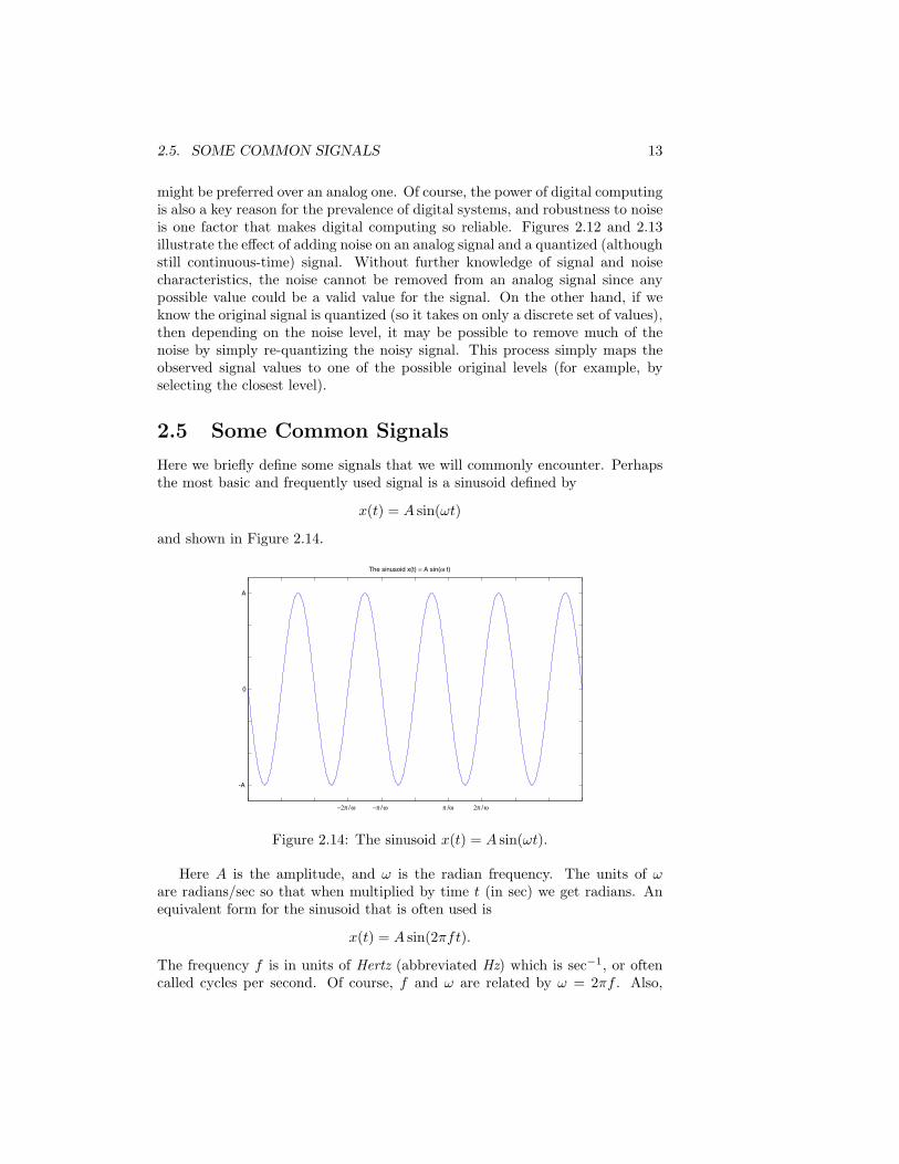
Here we briefly define some signals that we will commonly encounter. Perhapsthe most basic and frequently used signal is a sinusoid defined by

x(t) = A sin(ωt)

and shown in Figure 2.14.

-A

0

A

The sinusoid x(t) = A sin( ω t)

π / ω 2π / ω −π / ω −2π / ω

Figure 2.14: The sinusoid x(t) = A sin(ωt).

Here A is the amplitude, and ω is the radian frequency. The units of ωare radians/sec so that when multiplied by time t (in sec) we get radians. Anequivalent form for the sinusoid that is often used is

x(t) = A sin(2πft).

The frequency f is in units of Hertz (abbreviated Hz) which is sec−1, or oftencalled cycles per second. Of course, f and ω are related by ω = 2πf . Also,


it’s clear that since sin(θ + π/2) = cos θ, we could have equivalently written thesinusoid as

x(t) = A cos(2πft− π/2).

Up to this point, we have only considered real-valued signals. Althoughphysical quantities can generally be represented in terms of real-valued signals,it turns out to be extremely useful to consider signals taking on complex values.The most basic complex-valued signal we will use is the complex exponentialejωt. (Note that here we have used the symbol j instead of i to denote theimaginary number

√−1. This is common in electrical engineering since thesymbol i has traditionally been used to represent an electrical current.) Thewell-known Euler identity can be used to write the complex exponential in termsof standard sinusoids. Namely,

ejωt = cos(ωt) + j sin(ωt).

As with sinusoids, the complex exponential can also be written in terms offrequency in Hertz rather than radian frequency.

Some other signals that we will use on occasion and therefore give specialsymbols to are the step function, ramp, square wave, triangle wave, and the sincfunction (pronounced like “sink”). These signals are defined by

step(t) ={

0 if t < 01 if t ≥ 0

ramp(t) ={

0 if t < 0t if t ≥ 0

rect(t) ={

1 if − 1/2 ≤ t < 1/20 otherwise

tri(t) ={

1− |t| if − 1 ≤ t ≤ 10 otherwise

and

sinc(t) =sin(πt)

πt

and are shown in Figure 2.15.

2.6 Delta Functions

The notion of a delta function is extremely useful in the analysis of signalsand systems, although it may feel unnatural on first exposure. Although theconcept of the delta function can be made completely rigorous, rather than getside-tracked with too much mathematical detail and sophistication, our aimhere is to provide some intuition and ability to work with the delta function.On the other hand, it is important to have enough rigor so that this importanttool is used properly.

2.6. DELTA FUNCTIONS 15

-2 -1 0 1 2 -2

-1

0

1

2 step(t)

-2 -1 0 1 2 -2

-1

0

1

2 ramp(t)

-2 -1 0 1 2 -2

-1

0

1

2 rect(t)

-2 -1 0 1 2 -2

-1

0

1

2 tri(t)

-5 -4 -3 -2 -1 0 1 2 3 4 5 -0.5

0

0.5

1

sinc(t)

Figure 2.15: (a) Step function. (b) Ramp function. (c) Rectangle function. (d)Triangle function. (e) Sinc function.


The delta function in continuous-time is also called the Dirac delta function,unit impulse function, or sometimes just the impulse function. It is definedimplicitly through its behavior under integration as follows:

Definition: δ(t) is the Dirac delta function if it satisfies∫ ∞

−∞f(t)δ(t) dt = f(0) (2.1)

for every function f(t) that is continuous at t = 0.

From this definition we can infer the following two properties of the deltafunction. First, by considering the function f(t) = 1 in Equation (2.1), we get

∫ ∞

−∞δ(t) dt = 1 (2.2)

This result implies that the area under the delta function is equal to 1.The second property gives the value of δ(t) for t 6= 0. Suppose δ(t) took on

positive values in even a very small interval away from t = 0. Then we couldchoose a function f(t) that also took positive values inside a portion of this sameinterval, but with f(t) = 0 elsewhere (including t = 0) and with f(t) continuousat t = 0. However, in this case the left hand side of Equation (2.1) must bepositive, but the right hand side is 0. Therefore, δ(t) cannot take on positivevalues in any interval. A similar argument leads us to the conclusion that δ(t)cannot take on negative values in any interval. Thus, δ(t) = 0 for t 6= 0.

These two results (namely, that the area under δ(t) is 1 and that δ(t) = 0 forall t 6= 0) are inconsistent with our usual notions of functions and integration.If δ(0) was any finite value, then the area under δ(t) would be zero. Strictlyspeaking, δ(0) is undefined although it is convenient to think of δ(0) = ∞. Thus,although we call δ(t) the delta “function,” it is technically not a function in theusual sense. It is what is known as a distribution. However, it turns out thatfor many manipulations we can treat δ(t) like a function.

It is also convenient to have a graphical representation as shown in Figure2.16. The arrow indicates that the value at t = 0 is infinite (or undefined), withthe height of the arrow indicating the area under δ(t). To depict Aδ(t) whereA is some constant, we would draw the height of the arrow to be A.

It is sometimes also helpful to think of δ(t) as a limit of a sequence ofapproximating functions. Consider the function a rect(at). This has area 1, butif a > 1 it is more concentrated around t = 0. As we let a → ∞ we get asequence of approximations as shown in Figure 2.17, which intuitively get closerand closer to δ(t). In fact, it is not hard to verify that for f(t) continuous att = 0 we have ∫ ∞

−∞f(t) a rect(at) dt → f(0) as a →∞

so that in the limit a → ∞ the defining property of δ(t) is indeed satisfied.It turns out that many other choices for the approximating functions will alsowork if the area is 1 and scaling is done to get concentration at t = 0.


−1 −0.8 −0.6 −0.4 −0.2 0 0.2 0.4 0.6 0.8 10

0.5

1

1.5

2

2.5

3The delta function

Figure 2.16: Representation of a delta function.

-2 -1 0 1 2 0

0.5

1

1.5

2

2.5

3

3.5

4 a = 1/2

-2 -1 0 1 2 0

0.5

1

1.5

2

2.5

3

3.5

4 a = 1

-2 -1 0 1 2 0

0.5

1

1.5

2

2.5

3

3.5

4 a = 2

-2 -1 0 1 2 0

0.5

1

1.5

2

2.5

3

3.5

4

a = 4

Figure 2.17: The delta function is a limit of rectangle functions with area 1.


The primary motivation for introducing the delta function is that it is auseful tool in analyzing systems and signals as we’ll see in Chapter XX. Thereis also a physical motivation involving modeling of physical phenomena thatis actually closely related to the analytical motivation. In some situations wewould like to model physical phenomena that occur in a time interval shortcompared to the resolution of a measuring device. For example, we may beinterested in the energy entering a camera due to a flash of light as the camerashutter opens and closes very quickly. For a fixed shutter speed, many modelsfor the light source will be good enough to represent a “flash” or “impulse” oflight. However, if we fix a particular function to model the flash of light, it maynot represent a true “flash” for faster shutter speeds. Modeling the flash of lightas a delta function is an idealization that works for any (non-infinite) shutterspeed.

A number of properties of δ(t) can be obtained directly from the definition byutilizing the usual rules of integration. Intuition can also sometimes be gainedby considering approximations of δ(t), although a formal justification generallyrequires verifying the defining property.

For example, since δ(t) = 0 for all t 6= 0, it seems obvious that δ(t) is even.However, since δ(t) is technically not a function, we should really verify directlythat δ(−t) behaves just as δ(t) in the defining property of Equation (2.1). Thiscan be done by a simple change of variable as follows. For any function f(t)continuous at t = 0, we have

∫ ∞

−∞f(t)δ(−t) dt =

∫ ∞

−∞f(−u)δ(u) du = f(−u) |u=0= f(0)

where the first equality is obtained by the change of variable u = −t, and thesecond equality follows from the definition of δ(u). The conclusion is that δ(−t)satisfies the required property of δ(t), and so δ(−t) = δ(t).

By the change of variable u = at and considering the cases a > 0 and a < 0separately, it is easy to show that

δ(at) =1|a|δ(t).

By the change of variable u = t− t0, it follows that∫ ∞

−∞x(t)δ(t− t0) dt = x(t0).

Therefore, the time-shifted delta function δ(t−t0) behaves like we would expect.This property is sometimes called the sifting property of the delta function. Thenatural graphical depiction of δ(t− t0) is shown in Figure 2.18.

We now turn to the discrete-time delta function, also called the Kroneckerdelta function. The Kronecker delta function is denoted by δ[n] and defined as

δ[n] ={

1 if n = 00 otherwise


−1 −0.8 −0.6 −0.4 −0.2 0 0.2 0.4 0.6 0.8 10

0.5

1

1.5

2

2.5

3Time−shifted delta function, δ(t−0.6)

Figure 2.18: Time-shifted delta function.

−1 −0.8 −0.6 −0.4 −0.2 0 0.2 0.4 0.6 0.8 1−1

−0.5

0

0.5

1

1.5

2

2.5

3Discrete−time delta function

Figure 2.19: Discrete-time delta function.


Figure 2.19 shows the graph of δ[n]. Hence, in discrete-time, the delta func-tion is in fact a function in the proper sense. There are none of the mathematicalsubtleties/difficlties associated with the continuous-time delta function. In fact,δ[n] is rather simple to work with.

Many properties of δ(t) have analogous counterparts in discrete-time, andthe discrete-time properties are generally easier to verify. For example, theresult ∞∑

n=−∞f [n]δ[n] = f [0]

follows trivially from the definition. Recall that in continuous time, the anal-ogous property was actually the definition. Also trivial is the fact that δ[n] isan even function of n = . . . ,−1, 0, 1, . . .. It is easy to see that the time-shifteddelta function δ[n− n0] satisfies the discrete-time sifting property

∞∑n=−∞

f [n]δ[n− n0] = f [n0].

It turns out that for some properties the discrete-time counterpart is not anal-ogous. For example, in discrete-time if a is an integer we have δ[an] = δ[n].

2.7 2-D Signals

One useful notion that arises in two (and higher) dimensions is separability. Afunction f(x, y) is called separable if it can be written as f(x, y) = f1(x)f2(y).Many of the commonly encountered 2-D functions are simply separable exten-sions of the corresponding 1-D functions. For example, the 2-D version of thecomplex exponential is

ej(ω1x+ω2y) = ejω1xejω2y

where ω1 and ω2 are the radian frequencies in the x and y directions, respectively.That is, the 2-D complex exponential is simply the product of a 1-D complexexponential in each direction.

Likewise, the 2-D Dirac delta function δ(x, y) is given by

δ(x, y) = δ(x)δ(y)

Formally, δ(x, y) would actually be defined by the property∫ ∞

−∞

∫ ∞

−∞f(x, y)δ(x, y) dx dy = f(0, 0)

for any function f(x, y) continuous at (0, 0), but showing equivalence with theseparable expression is straightforward.

Similarly, in the discrete case, the Kronecker delta δ[m,n] is defined by

δ[m,n] ={

1 if m = n = 00 otherwise

2.7. 2-D SIGNALS 21

Clearly the Kronecker delta is also separable

δ[m,n] = δ[m]δ[n].

Many other 2-D functions like rect(x, y) and sinc(x, y) have natural separableextensions from the 1-D versions as well.

Separability can offer some nice analytical and computational advantages.For example, terms involving the two independent variables can sometimes beseparated, reducing a two-dimensional analysis to two separate one-dimensionalanalyses. This can result in computational savings by allowing processing to bedone along the two dimensions separately.

basics of signals - princeton university

Documents

signal fx

function fx

time t

function of time ft

function of depth

signal need

signal analysis

signal processing