batch: machine learning inference serving on serverless
TRANSCRIPT
BATCH: Machine Learning Inference Serving onServerless Platforms with Adaptive Batching
Ahsan Ali§
University of Nevada, RenoReno, NV
Riccardo Pinciroli§
William and MaryWilliamsburg, VA
Feng YanUniversity of Nevada, Reno
Reno, [email protected]
Evgenia SmirniWilliam and MaryWilliamsburg, VA
Abstract—Serverless computing is a new pay-per-use cloudservice paradigm that automates resource scaling for statelessfunctions and can potentially facilitate bursty machine learningserving. Batching is critical for latency performance and cost-effectiveness of machine learning inference, but unfortunately itis not supported by existing serverless platforms due to theirstateless design. Our experiments show that without batching,machine learning serving cannot reap the benefits of serverlesscomputing. In this paper, we present BATCH, a frameworkfor supporting efficient machine learning serving on serverlessplatforms. BATCH uses an optimizer to provide inference taillatency guarantees and cost optimization and to enable adaptivebatching support. We prototype BATCH atop of AWS Lambdaand popular machine learning inference systems. The evaluationverifies the accuracy of the analytic optimizer and demonstratesperformance and cost advantages over the state-of-the-art methodMArk and the state-of-the-practice tool SageMaker.
Index Terms—Machine-learning-as-a-service (MLaaS), Infer-ence, Serving, Batching, Cloud, Serverless, Service Level Objec-tive (SLO), Cost-effective, Optimization, Modeling, Prediction
I. INTRODUCTION
Serverless (also referred to as Function-as-a-Service (FaaS)or cloud function services) is an emerging cloud paradigmprovided by almost all public cloud service providers, in-cluding Amazon Lambda [1], IBM Cloud Function [2], Mi-crosoft Azure Functions [3], and Google Cloud Functions[4]. Serverless offers a true pay-per-use cost model and hidesinstance management tasks (e.g., deployment, scaling, moni-toring) from users. Users only need to provide the functionand its trigger event (e.g., HTTP requests, database uploads),as well as a single control system parameter memory sizethat determines the processing power, allocated memory, andnetworking performance of the serverless instance. Intelligenttransportation systems [5], IoT frameworks [6–8], subscriptionservices [9], video/image processing [10], and machine learn-ing tools [11–13] are already being deployed on serverless.
Machine Learning (ML) Serving. ML applications havetypically three phases: model design, model training, andmodel inference (or model serving).1. In the model designphase, the model architecture is designed manually or throughautomated methods [14, 15]. Then, the crafted model withinitial parameters (weights) is trained iteratively until con-vergence. A trained model is published in the cloud to pro-vide inference services, such as classification and prediction.
§Both authors contributed equally to this research.1We use the terms model serving and model inference interchangeably
Among the three phases, model serving has a great potentialto benefit from serverless because the arrival intensity ofclassification/prediction requests is dynamic and their servinghas strict latency requirements.
Serverless vs. IaaS for ML Serving. Serverless com-puting simplifies the deployment process of ML Serving asapplication developers only need to provide the source-codeof their functions without worrying about virtual machine(VM) resource management, such as (auto)scaling and loadbalancing. Despite the great capabilities of serverless, existingworks show that in public clouds, the serverless paradigmfor ML serving is more expensive compared to IaaS [16, 17].Recent works have shown that it is possible to use serverlessto improve the high cost for ML serving [16, 18] but ignoreone important feature of serving workloads in practice: bursti-ness [19,20]. Bursty workloads are characterized by time peri-ods of low arrival intensities that are interleaved with periodsof high arrival intensities. Such behavior makes the VM-basedapproach very expensive: over-provisioning is necessary to ac-commodate sudden workload surges (otherwise, the overheadof launching new VMs, which can be a few minutes long, maysignificantly affect user-perceived latencies). The scaling speedof serverless can solve the sudden workload surge problem.In addition, during low arrival intensity periods, serverlesscontributes to significant cost savings, thanks to its pay-per-usecost model.
Serverless for ML Serving: Opportunities and Chal-lenges. Another important factor that heavily impacts bothcost and performance of ML serving inference is batching[16,21]. With batching, several inference requests are bundledtogether and served concurrently by the ML application. Asrequests arrive, they are served in a non-work-conserving way,i.e., they wait in the queue till enough requests form a batch.In contrast to batch workloads in other domains that aretypically treated as background tasks [22–25], batching forML inference serving is done online, as a foreground process.Batching dramatically improves inference throughput as the in-put data dimension determines the parallelization optimizationopportunities when executing each operator according to thecomputational graph [26,27]. Provided that the monetary costof serverless on public cloud is based on invocations, a fewlarge batched requests are cheaper than many small individualrequests. Therefore, judicious parameterization of batching canpotentially improve performance while reducing cost.
SC20, November 9-19, 2020, Is Everywhere We Are978-1-7281-9998-6/20/$31.00 ©2020 IEEE
Due to the stateless property of serverless design, i.e.,no data (state) is kept between two invocations, batchingis not supported as a native feature within the serverlessparadigm. An additional challenge is that batching introducestwo configuration parameters: batch size (i.e., the maximumnumber of requests to form a batch) and timeout (i.e., themaximum time it allows to wait for requests to form the batch).These parameters need to be adjusted on the fly according tothe arrival intensity of inference requests to meet inferencelatency SLOs. The performance and cost effectiveness ofbatching depends strongly on the judicious choice of the aboveparameters. No single parameter choice can work optimally forall workload conditions.
Our Contribution. Here, we address the above challengesby developing an autonomous framework named BATCH [28].The first key component of BATCH is a dispatching bufferthat enables batching support for ML serving on serverlessclouds. BATCH supports automated adaptive batching andits associated parameter tuning to provide tail latency per-formance guarantees and cost optimization while maintaininglow system overhead. We develop a lightweight profiler thatfeeds a performance optimizer. The performance optimizer isdriven by a new analytical methodology considers the salientcharacteristics of bursty workloads, serverless computing, andML serving to estimate inference latencies and monetary cost.
We prototype BATCH atop of AWS Lambda and evalu-ate its effectiveness using different ML serving frameworks(TensorFlow Serving and MXNet Model Server) and imageclassification applications (MoBiNet, Inception-v4, ResNet-18, ResNet-50, and ResNet-v2) driven both by synthetic andreal workloads [29,30]. Results show that the estimation accu-racy of the analytical model is consistently high (average erroris lower than 9%) independent of the considered system con-figurations (i.e., framework, application, memory size, batchsize, and timeout). Controlling the configuration parameters onthe fly, BATCH outperforms SageMaker [31] (the state-of-the-practice), MArk [16] (the state-of-the-art), and vanilla Lambdafrom both cost and performance viewpoints. More importantly,BATCH supports a full serverless paradigm for online MLserving, enabling fully automated and efficient SLO-aware MLserving deployment on public clouds.
II. MOTIVATION AND CHALLENGES
We discuss the potential advantages of using serverless forML serving and summarize its open challenges.
A. ML Serving Workload is Bursty
Workload burstiness is omnipresent in non-laboratory set-tings [32–35]. Past work has showed that if burstiness is notincorporated into performance models, the quality of theirprediction plummets [36, 37].
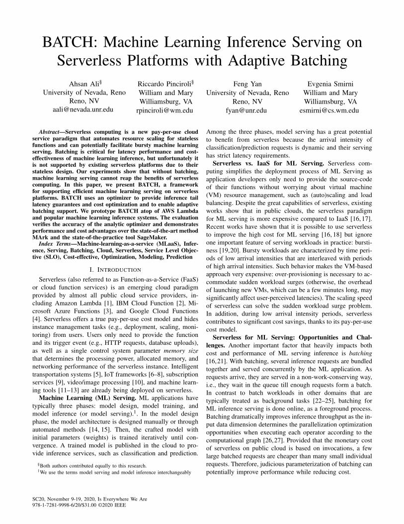
Fig. 1(a) plots the arrival intensity of cars passing throughthe New York State (NYS) Thruway during three businessdays in the fourth quarter of 2018 [29]. This trace representsa typical workload of an image recognition application thatdetects the plate of vehicles that pass under a checkpoint
0
5
10
15
20
06:00 12:00 18:00Arr
ival In
tensi
ty [
r/s]
time
Oct. 08Oct. 09
Nov. 16
(a) NYS Thruway
0
50
100
150
06:00 12:00 18:00Arr
ival In
tensi
ty [
r/s]
time
Feb. 14Feb. 15
May 25
(b) Twitter
Fig. 1: Real-world traces from [29] and [30].
[18]. The three days have distinct arrival intensities that arenon-trivial to accurately predict. Distinct traffic peaks are alsoobserved in a Twitter trace [30] that represents a typical arrivalof tweets processed for sentiment analysis that has been usedfor ML serving elsewhere [16]. Fig. 1(b) shows the arrivalintensity of three distinct days in the first semester of 2017.Observation #1. ML inference application often have burstyarrivals. Burstiness must be incorporated into the design ofany framework for performance optimization.
B. Why Serverless for ML Serving
There are two types of approaches to cope with suddenworkload surges: resource over-provisioning and autoscaling.For bursty workloads, resource over-provisioning is not cost-effective as the difference between high and low intensitiescan be dramatic and lots of paid computing resource is leftidle for extensive periods.
Autoscaling is the current industry solution: Amazon’sSageMaker [31] facilitates ML tasks and supports AWS au-toscaling [38]. With SageMaker, users can define scalingmetrics such as when and how much to scale.
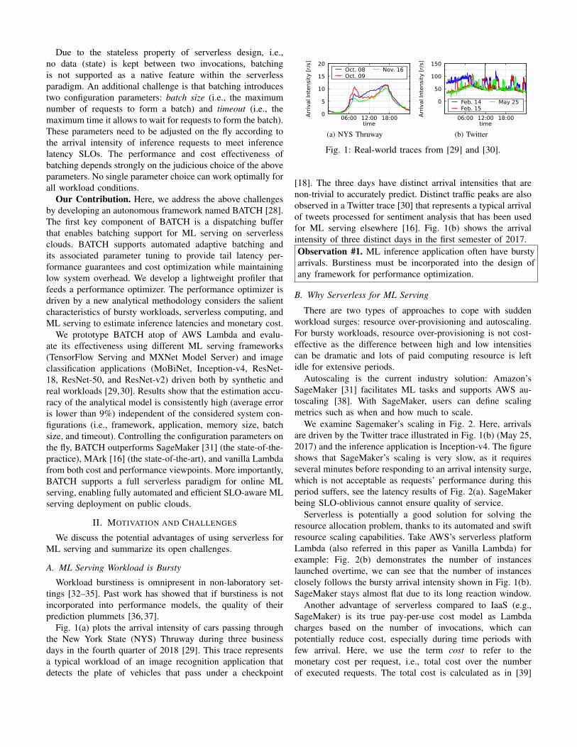
We examine Sagemaker’s scaling in Fig. 2. Here, arrivalsare driven by the Twitter trace illustrated in Fig. 1(b) (May 25,2017) and the inference application is Inception-v4. The figureshows that SageMaker’s scaling is very slow, as it requiresseveral minutes before responding to an arrival intensity surge,which is not acceptable as requests’ performance during thisperiod suffers, see the latency results of Fig. 2(a). SageMakerbeing SLO-oblivious cannot ensure quality of service.
Serverless is potentially a good solution for solving theresource allocation problem, thanks to its automated and swiftresource scaling capabilities. Take AWS’s serverless platformLambda (also referred in this paper as Vanilla Lambda) forexample: Fig. 2(b) demonstrates the number of instanceslaunched overtime, we can see that the number of instancesclosely follows the bursty arrival intensity shown in Fig. 1(b).SageMaker stays almost flat due to its long reaction window.
Another advantage of serverless compared to IaaS (e.g.,SageMaker) is its true pay-per-use cost model as Lambdacharges based on the number of invocations, which canpotentially reduce cost, especially during time periods withfew arrival. Here, we use the term cost to refer to themonetary cost per request, i.e., total cost over the numberof executed requests. The total cost is calculated as in [39]
0
2
4
6
8
10
0 700 1400
Late
ncy
[se
c]
Time [min]
Lambda Sagemaker
(a) Latency
20
40
60
80
100
0 700 1400 3
6
9
12
15
Concu
rrent
fucn
tions
Insta
nce
count
Time [min]
Lambda Sagemaker
(b) Instance count
0
0.35
0.7
Avg. C
ost
[$
/r]
(10
-4)
Lambda Sagemaker
(c) Cost
Fig. 2: Performance of inference using Inception-v4 deployed on SageMaker (with instance type c5.4xlarge) and Lambda. Thenumber of instances used by Sagemaker varies between 5 to 11 based on the workload intensity.
without considering the free tier (i.e., free invocations andcompute time available every month):
CLambda = (S ·M · I) ·K1 + I ·K2, (1)
where S is the length of the function call (referred as batchservice time here), M is the memory allocated for the function,I is the number of calls to the function that decreases whenrequests are batched together, K1 (i.e., 1.66667 ·10−5 $/GB-s)is the cost of the memory, and K2 (i.e., 2 ·10−7 $) is the costof each call to the function. This is different from the AWSEC2 cost, i.e., CEC2 = K ·H, that only accounts for the costper hour of an instance (K) and the number of power-on hoursof the instance (H).Observation #2. Compared to IaaS solutions (autoscaling),serverless computing is very agile, which is critical for per-formance during time periods of bursty workload conditions.In addition, the quick scale down and pay-per-use cost modelcontributes to the cost-effectiveness of serverless.
C. The State of the Art
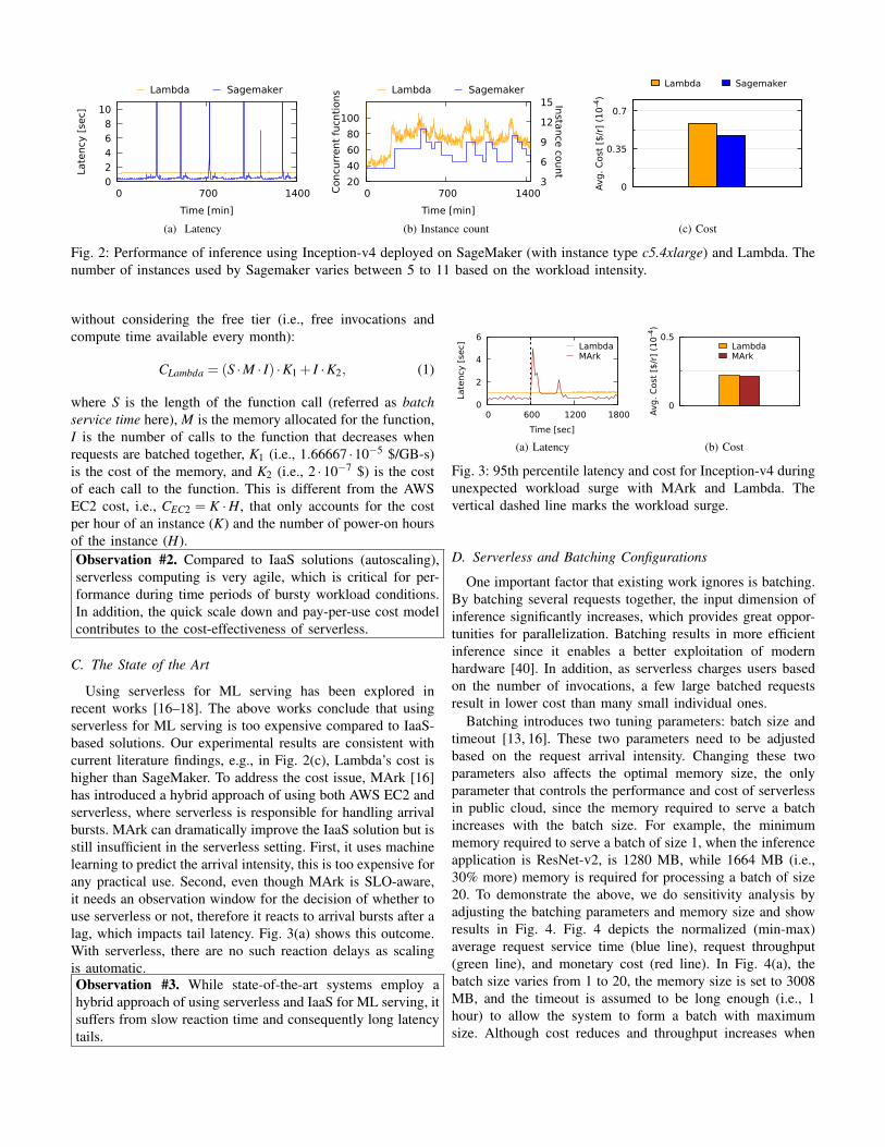
Using serverless for ML serving has been explored inrecent works [16–18]. The above works conclude that usingserverless for ML serving is too expensive compared to IaaS-based solutions. Our experimental results are consistent withcurrent literature findings, e.g., in Fig. 2(c), Lambda’s cost ishigher than SageMaker. To address the cost issue, MArk [16]has introduced a hybrid approach of using both AWS EC2 andserverless, where serverless is responsible for handling arrivalbursts. MArk can dramatically improve the IaaS solution but isstill insufficient in the serverless setting. First, it uses machinelearning to predict the arrival intensity, this is too expensive forany practical use. Second, even though MArk is SLO-aware,it needs an observation window for the decision of whether touse serverless or not, therefore it reacts to arrival bursts after alag, which impacts tail latency. Fig. 3(a) shows this outcome.With serverless, there are no such reaction delays as scalingis automatic.Observation #3. While state-of-the-art systems employ ahybrid approach of using serverless and IaaS for ML serving, itsuffers from slow reaction time and consequently long latencytails.
0
2
4
6
0 600 1200 1800
Late
ncy
[se
c]
Time [sec]
LambdaMArk
(a) Latency
0
0.5
Avg
. C
ost
[$
/r]
(10
-4)
LambdaMArk
(b) Cost
Fig. 3: 95th percentile latency and cost for Inception-v4 duringunexpected workload surge with MArk and Lambda. Thevertical dashed line marks the workload surge.
D. Serverless and Batching Configurations
One important factor that existing work ignores is batching.By batching several requests together, the input dimension ofinference significantly increases, which provides great oppor-tunities for parallelization. Batching results in more efficientinference since it enables a better exploitation of modernhardware [40]. In addition, as serverless charges users basedon the number of invocations, a few large batched requestsresult in lower cost than many small individual ones.
Batching introduces two tuning parameters: batch size andtimeout [13, 16]. These two parameters need to be adjustedbased on the request arrival intensity. Changing these twoparameters also affects the optimal memory size, the onlyparameter that controls the performance and cost of serverlessin public cloud, since the memory required to serve a batchincreases with the batch size. For example, the minimummemory required to serve a batch of size 1, when the inferenceapplication is ResNet-v2, is 1280 MB, while 1664 MB (i.e.,30% more) memory is required for processing a batch of size20. To demonstrate the above, we do sensitivity analysis byadjusting the batching parameters and memory size and showresults in Fig. 4. Fig. 4 depicts the normalized (min-max)average request service time (blue line), request throughput(green line), and monetary cost (red line). In Fig. 4(a), thebatch size varies from 1 to 20, the memory size is set to 3008MB, and the timeout is assumed to be long enough (i.e., 1hour) to allow the system to form a batch with maximumsize. Although cost reduces and throughput increases when

Request Service Time Request Throughput Monetary Cost
0
0.2
0.4
0.6
0.8
1
0 4 8 12 16 20
Batch Size
(a) Timeout = 1 hr, Memory = 3008 MB
0
0.2
0.4
0.6
0.8
1
0 0.1 0.2 0.3
Timeout [s]
(b) Batch Size = 20, Memory = 3008 MB
0
0.2
0.4
0.6
0.8
1
1.5 2 2.5 3
Memory Size [GB]
(c) Batch Size = 5, Timeout = 1 hr
Fig. 4: Effect of batch size, timeout, and memory size on average request service time, request throughput, and monetary costof ResNet-v2 deployed on AWS Lambda. Service time, throughput, and cost are normalized (min-max).
batch size increases, request processing times suffer as earlierrequests need to wait until the entire batch is formed. Similarconsiderations may be drawn when timeout varies, see Fig.4(b). It is worth noting that for the considered configuration,the timeout effect on the system performance decreases whenit is longer than 0.2 seconds. Long timeouts allow reachingthe maximum batch size easier, especially if the batch size issmall. Fig. 4(c) depicts the system performance as a functionof the memory size, when the batch size is 5, and the timeout islong enough to guarantee that all requests are collected (e.g., 1hour). Here, monetary cost is not monotonous since it dependson both memory size and the batch service time, see Eq. (1). InFig. 4(c), both these parameters are varying at the same timegiven that the processing time decreases with more memory.Observation #4. The effectiveness of batching strongly de-pends on its parameterization.
E. Challenges of ML Serving on Serverless
Despite the great potential of using serverless for MLserving, there are several challenges that need to be addressedto enable efficient ML serving on serverless:
No batching support: As shown in Section II-C, batchingcan drastically improve the performance [21] and monetarycost of ML serving. However, existing serverless platformsin public clouds do not support this important feature due toits stateless design, i.e., no data (state) can be stored betweentwo invocations. To solve this challenge, we extend the currentserverless design to allow for a dispatching buffer so thatrequests can form a batch before processing.
SLO-oblivious: ML serving usually has strict latency SLOrequirements to provide good user experience. Past studieshave shown that if latency increases by 100 ms, revenue dropsby 1% [41]. Existing serverless platforms in public cloudsare SLO-oblivious and do not support user specified latencyrequirements. We are motivated to develop a performance opti-mizer that can support strict SLO guarantees and concurrentlyoptimize monetary cost.
Adaptive parameter tuning: To support user defined SLOwhile minimizing monetary cost, memory size (the singleserverless parameter) and batching parameters need to bedynamically adjusted (optimized) according to the intensity of
Service TimeModel
Profiler
Arrivalprocess
PerformanceOptimizer
ServerlessPlatform
Workload
● Batch Size● Timeout [s]
● Memory Size [MB]
SLOsBudget
BatchDispatching
Buffer
BATCH1a
3
5 6
Empirical Measurementsof Arrival Process
1b
2a 2b
4a
4b
Empirical Measurementsof Service Times
Fig. 5: Overview of BATCH.
arrival requests. There is no existing method that can optimizethe above parameters on-the-fly. We are motivated to developan optimization methodology that can continuously tune theseparameters to provide SLO support.
Lightweight: Given that the cost model of serverless is pay-per-use, the aforementioned optimization methodology needsto be lightweight. Such requirement excludes learning orsimulation based approaches. We are thus motivated to buildthe optimization methodology using analytical models.
III. BATCH DESIGN
BATCH determines the best system configuration (i.e.,memory size, maximum batch size, and timeout) to meet user-defined SLOs while reducing the cost of processing requestson a serverless platform. The workflow of BATCH is shownin Fig. 5. Initially, BATCH feeds the Profiler with empiricalmeasurements of the workload arrival process 1a and servicetimes 1b . The Profiler uses the KPC-toolbox [42] to fit thesequence of arrivals into a stochastic process 2a and usessimple regression to capture the relationship between systemconfiguration and request service times 2b . Using as inputsthe fitted arrival process, request service times for differentsystem configurations, the monetary budget, and the userSLO, BATCH uses an analytic model implemented withinthe Performance Optimizer component to predict the distri-bution of latencies 3 and determines the optimal serverlessconfiguration to reach specific performance/cost goals while

complying with a published SLO. The optimal batch sizeand timeout are communicated to the Buffer 4a , while theoptimal memory size is allocated to the function deployed onthe serverless platform 4b . The Buffer uses the parametersprovided by the Performance Optimizer to group incomingrequests into batches 5 . Once the batch size is reached orthe timeout expires, the accumulated requests are sent fromthe Buffer to the serverless platform for processing 6 . Furtherdetails are provided for each component of BATCH below.
A. Profiler
To determine the workload arrival process, the Profilerobserves the inter-arrival times of incoming requests. BATCHuses the KPC-Toolbox [42] to fit the collected arrival trace intoa Markovian Arrival Process (MAP) [43], a class of processesthat can capture burstiness. To profile the inference time onthe serverless platform, the Profiler measures the time requiredto process batches of different sizes for certain amounts ofallocated memory. BATCH derives the batch service timemodel using multivariable polynomial regression [44] andassuming that inference times are deterministic. Past work hasshown that inference service times are deterministic [45], ourexperiments (see Section VI-B) confirm this.
B. Buffer
Since serverless platforms do not automatically allow pro-cessing multiple requests in a single batch, BATCH imple-ments a Buffer to batch together requests for serving. Theperformance optimizer determines the optimal batch size basedon the arrival process, service times, SLO, and budget. Theperformance optimizer also defines a timeout value that isused to avoid waiting too long for collecting enough requests.Therefore, a batch is sent to the serverless platform as soonas either the maximum number (batch size) of requests iscollected or timeout expires.
C. Performance Optimizer
The Performance Optimizer is the core component ofBATCH. It uses the arrival process and service time (bothestimated by the profiler) to predict the time required toserve the incoming requests. Using the SLO and the availablebudget (both provided by the user), the performance optimizerdetermines which system configuration (i.e., memory size,batch size, and timeout) allows minimizing the cost (latency)while meeting SLOs on system performance (budget). To solvethis optimization problem, BATCH uses an analytical approachthat allows predicting the request latency distribution.
We opt for an analytical approach as opposed to simulationor regression for the following reasons. Analytical models aresignificantly lightweight, i.e., they do not require extensiverepetitions to obtain results within certain confidence intervalsas simulation does. Equivalently, they do not require extensiveprofiling experiments that regression traditionally requires.
IV. PROBLEM FORMULATION AND SOLUTION
Since SLOs are typically defined as percentiles [46,47], themodel must determine the request latency distribution whileaccounting for memory size, batch size, timeout, and arrivalintensity. Since the model is analytical, no training is required.
The challenges for developing an analytical model here arethree-fold: 1) the model needs to effectively capture burstinessin the arrival process for a traditional infinite server [48] thatcan model the serverless paradigm (i.e., there is no inherentwaiting in a queue), 2) the model needs to effectively capturea deterministic service process which is challenging [45, 49],and 3) needs to predict performance in the form of latencypercentiles [46, 47], this is very challenging since analyticalmodels typically provide just averages [45, 50]. In the fol-lowing, we give an overview of how we overcome the abovechallenges.Problem Formulation:BATCH optimizes system cost by solving the following:
minimize Cost
subject to Pi ≤ SLO,(2)
where Cost, given by Eq. (1), is the price that the systemcharges to process the incoming requests and Pi is the ith-percentile latency that must be shorter than the user-definedSLO. BATCH can minimize the request latency by solving:
minimize Pi
subject to Cost≤ Budget,(3)
where Budget is the maximum price for serving a singlerequest. These optimization problems allow minimizing eitherlatency or cost (at the expense of the other measure, whichmust comply with the given target). The optimization in Eqs.(2) and (3) are solved via exhaustive search within a spacethat is quickly built by the analytical model (see Section V).Analytical Model:In order to determine the optimal system configuration, (i.e.,the memory size, the maximum batch size B, and the timeoutT ) BATCH first evaluates the distribution of jobs in the Bufferby observing the arrival process. The probability that a batchof size k is processed by the serverless function is equal to theprobability that k ≤ B requests are into the buffer by time T .In the following, we show how the prediction model operateswith different arrival processes.Poisson arrival process. We start with the simplest case wherethe arrival process is a Poisson distribution with rate λ and itis represented by the following B×B matrix:
QQQ =
−λ λ
. . . . . .−λ λ
0
. (4)
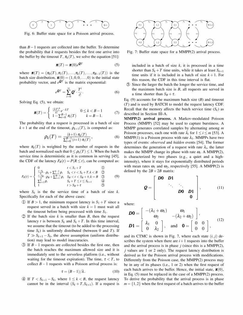
The state space of the buffer is represented by the continuoustime Markov chain (CTMC) shown in Fig. 6. Since the timeoutstarts when the first request arrives at the buffer, each state i ofthe CTMC represents the buffer with i+1 requests. No more
0 1 2 B-1
λ λ λ λ
Fig. 6: Buffer state space for a Poisson arrival process.
than B−1 requests are collected into the buffer. To determinethe probability that k requests besides the first one arrive intothe buffer by the timeout T , πk(T ), we solve the equation [51]:
πππ(T ) = πππ(0)eQQQT (5)
where πππ(T ) = (π0(T ),π1(T ), . . . ,πk(T ), . . . ,πB−1(T )) is thebatch size distribution, πππ(0) = (1,0,0, . . . ,0) is the initial stateprobability vector, and eQQQT is the matrix exponential:
eQQQT =∞
∑i=0
QQQi · Ti
i!. (6)
Solving Eq. (5), we obtain:
πππ(T ) =
{(λT )k
k! e−λT 0≤ k < B−11−∑
B−1i=0 πi(T ) k = B−1.
(7)
The probability that a request is processed in a batch of sizek+1 at the end of the timeout, ρk+1(T ), is computed as:
ρk(T ) =(k+1)·πk(T )
∑B−1i=0 (i+1)·πi(T )
, (8)
where πk(T ) is weighted by the number of requests in thebatch and normalized such that 0≤ ρk(T )≤ 1. When the batchservice time is deterministic as it is common in serving [45],the CDF of the latency FR(t) = P(R≤ t), can be computed as:
FR(t) =
0 t < S1 +T 1t−Sk
T ·ρk +∑k−1i=1 ρi Sk < t < Sk +T,k < B 2
t−SBτ·ρB +∑
B−1i=1 ρi SB < t < SB + τ,k = B 3
∑ki=1 ρi Sk +T ≤ t ≤ Sk+1 4
1 t > SB + τ 5
(9)
where Sk is the the service time of a batch of size k.Specifically for each of the above cases:
1 If B > 1, the minimum request latency is S1 +T since arequest served in a batch with size k = 1 must wait allthe timeout before being processed with time S1.
2 If the batch size k is smaller than B, then the requestlatency t is between Sk and Sk +T . In this time interval,we assume that the timeout (to be added to the processingtime Sk) is uniformly distributed (between 0 and T ). IfT � Sk+1− Sk, the above assumption (uniform distribu-tion) may lead to model inaccuracies.
3 If B−1 requests are collected besides the first one, thenthe batch reaches the maximum allowed size and it isimmediately sent to the serverless platform (i.e., withoutwaiting for the timeout expiration). The time, τ < T , tocollect B−1 requests with a Poisson arrival process is:
τ = (B−1)/λ . (10)
4 If T < Sk+1− Sk, where 1 ≤ k < B, the request latencycannot be in the interval (Sk + T,Sk+1). If a request is
0,1 1,1 2,1 B-1,1
λ1 λ1 λ1
0,2 1,2 2,2 B-1,2
λ2 λ2 λ2 λ2
λ1
!2 !2 !2 !2!1 !1 !1 !1
Fig. 7: Buffer state space for a MMPP(2) arrival process.
included in a batch of size k, it is processed in a timeshorter than Sk +T time units, while it takes at least Sk+1time units if it is included in a batch of size k+ 1. Forthis reason, the CDF in this time interval is flat.
5 Since the larger the batch the longer the service time, andthe maximum batch size is B, all requests are served ina time shorter than SB + τ .
Eq. (9) accounts for the maximum batch size (B) and timeout(T ) and is used by BATCH to model the request latency CDF.Recall that the memory affects the batch service time (Sk) asdescribed in Section III-A.MMPP(2) arrival process. A Markov-modulated PoissonProcess (MMPP) [52] may be used to capture burstiness. AMMPP generates correlated samples by alternating among mPoisson processes, each one with rate λi for 1≤ i≤m [53]. AMMPP(1) is a Poisson process with rate λ1. MMPPs have twotypes of events: observed and hidden events [54]. The formerdetermines the generation of a request with rate λi, the lattermakes the MMPP change its phase with rate ωi. A MMPP(2),is characterized by two phases (e.g., a quiet and a high-intensity), where it stays for exponentially distributed periodswith mean rates ω1 and ω2, respectively [55]. A MMPP(2) isdefined by the 2B×2B matrix:
QQQ =
DDD000 DDD111
. . . . . .DDD000 DDD111
000
, (11)
where:
DDD000 =
[−(λ1 +ω1) ω1
ω2 −(λ2 +ω2)
],
DDD111 =
[λ1 00 λ2
], and 000 =
[0 00 0
],
(12)
and its CTMC is shown in Fig. 7, where each state (i, j) de-scribes the system when there are i+1 requests into the bufferand the arrival process is in phase j (since this is a MMPP(2),j values are 1 or 2 only). The request latency distribution isderived as for the Poisson arrival process with modifications.Differently from the Poisson case, the MMPP(2) process maybe in any of its phases (i.e., 1 or 2) when the first request ofeach batch arrives to the buffer. Hence, the initial state, πππ(0),in Eq. (5) must be replaced in the case of a MMPP(2) process.To derive the probability that the arrival process is in phasem= {1,2} when the first request of a batch arrives to the buffer

0,1 1,1 2,1 B-1,1
λ1 λ1 λ1
0,2 1,2 2,2 B-1,2
λ2 λ2 λ2 λ2
λ1
!2 !2 !2 !2!1 !1 !1 !1
λ12 λ12 λ12 λ12
λ21 λ21 λ21λ21
Fig. 8: Buffer state space of a MAP(2) arrival process.
we proceed as follows. First, we derive the average numberof requests generated during each phase, evm = λm/ωm, as theproduct of the request arrival rate, λm, and the average durationof each phase, 1/ωm. Then, we compute the average numberof times that the buffer is in state (0,m) when the first requestof a batch arrives. Knowing that evm is the number of requestsgenerated during phase m, we divide it by the expected batchsize:
αm =evm
min(B,λm ·T +1). (13)
The initial state, πππ(0), to be used in Eq. (5) in the MMPP(2)case, is computed as:
πππ(0) =(
α1
α1 +α2,
α2
α1 +α2
). (14)
With a MMPP(2) arrival process, also the required time, τ , tocollect B− 1 requests besides the first one (i.e., the time toreach the maximum batch size) is different from the Poissoncase since it depends on the arrival process. Hence, Eq. (10)in case 3 of the proposed model, i.e., Eq. (9), needs to bereplaced by:
τ = (B−1) · ω1 +ω2
λ1 ·ω2 +λ2 ·ω1. (15)
MAP(2) arrival process. MAPs are flexible non-renewalstochastic processes that can model general distributions andare commonly used to describe correlated and bursty events[50, 56–59]. MAPs are a generalization of MMPPs [52] thatallows changing a phase also during observed events. A two-phase MAP is defined by the matrix in Eq. (11), where:
DDD000 =
[−(λ1 +λ12 +ω1) ω1
ω2 −(λ2 +λ21 +ω2)
]and DDD111 =
[λ1 λ12λ21 λ2
],
(16)
and the state space of the buffer is represented by the CTMCin Fig. 8. A MAP(2) is defined by four parameters (i.e.,mean, square coefficient of variation, skewness, and lag-1autocorrelation) and can easily fit bursty traces [60]. Therequest latency distribution with a MAP(2) arrival process iscomputed with the exact same steps as for the MMPP(2) case.
V. PROTOTYPE IMPLEMENTATION
We prototype BATCH atop AWS Lambda and discuss theimplementation choices for its key components in this section.
Serving package development and deployment. We de-velop the serving package according to the guidelines provided
by AWS [61]. The serving package is implemented using twowidely used ML frameworks, Tensorflow [26] and MXNetModel Server [62]. A function is created using the cre-ate function method from the boto3 library [63] for deployingthe package. We minimize the invocation delay by 2× throughpersisting the model graphs in memory.
Serverless Inference. Once the function is created and thepackage is deployed, the framework is ready for serving. Theserving function takes incoming requests (e.g., images) asinputs in the form of a list, each item on the list represents arequest. As soon as the function is invoked, the list of requestsare transformed into a batch by the serving function and thebatched requests are processed through the ML model forinference. For each request, typically the top inferred valueis returned from the model and sent back to the end users.
Profiler. The most time consuming task of the Profiler ismeasuring the service time of the ML application under differ-ent system configurations (i.e., memory size, batch size, andtimeout). To reduce the profiling time, the Profiler measuresthe workload service time under only a few different systemconfigurations and estimates service times of the remainingones through regression. We prototype the Profiler atop ofAWS CloudWatch [64]. Since this is an offline phase andthe profiler requires little computational power, it can becollocated with the Buffer and Performance optimizer.
Buffer. The buffer module uses a proxy server to collectincoming requests to form a batch. The proxy server requireslittle computational power and can be deployed on a cheapburstable instance (e.g., t2.nano [65], less than 0.14 $/day)along with the Profiler. Alternatively, the buffer can be im-plemented using the streaming service offered by AWS (e.g.,Amazon Kinesis [66]) but at the premium charged by AWS.
Performance optimizer. The performance optimizer imple-ments the model described in Section IV to determine the bestsystem configuration based on the actual workload intensity.The analytical model can be collocated with the Profiler andBuffer. It quickly builds the state space of all considered con-figuration options and selects the optimal system configurationin less than 10 seconds. Figure 9 shows the CPU and memoryusage of an AWS t2.nano instance ($0.14/day) hosting BATCHcomponents. The maximum memory utilization is less than200 MB (over 512 MB available for a t2.nano instance). Sincethe optimizer runs every hour and takes less than 10 secondsto find an optimal solution, CPU utilization is negligible. Thecomputation time of BATCH depends only on the number ofexplored configurations and is not affected by the intensity ofthe arrival process since the state space is finite.
VI. RESULTS
Here, we evaluate the accuracy of the multivariable polyno-mial model for the estimation of the batch service time (seeSection III-A). BATCH is validated experimentally on AWSLambda and compared to other available strategies.
A. Experimental Setup
We evaluate BATCH with two ML Serving Frameworks:

0
25
50
75
100
0 1 2 3 0
128
256
384
512
CPU
Uti
l. [
%]
Mem
. Util. [M
B]
time [hr.]
CPU Memory
Fig. 9: CPU and memory usage over three hours of an AWSt2.nano instance hosting BATCH components. The daily costof a t2.nano instance is less than $0.14.
0 50
100 150 200 250 300
0 0.5 1Arr
ival In
tensi
ty [
r/s]
time [hr]
MMPP(2)1 MMPP(2)2
(a) Arrival rate of MMPPs
0
50
100
150
200
250
06:00 12:00 18:00Arr
ival In
tensi
ty [
r/s]
time
NYS ThruwayTwitter
(b) Arrival rate of real traces
Fig. 10: Intensity of arrival processes used to evaluate BATCH.
• TensorFlow [26] is a widely adopted ML framework whichsupports a wide range of ML applications such as imageclassification, speech recognition, and more. We are unableto use the TensorFlow serving due to package size limita-tions (250 MB) imposed by AWS Lambda. We implementour own serving system based on TensorFlow.
• MXNet Model Server [62] is a popular ML framework thatsupports a wide range of ML applications. MXNet doesnot inherently support dynamic batch size for inference. Weextend MXNet for dynamic batching.
ML Applications. We use popular computer vision MLmodels with serving requests extracted from the ImageNet-22K dataset [67] (image resolution: 224 ×224×3):• MoBiNet [68] is a Mobile Binary Network for lightweight
image classification.• ResNet-18 and ResNet-50 [69] are medium size models with
residual functions (18 and 50 layers, repsectively).• Inception-v4 [70] is a large deep convolutional neural net-
work (48 layers) with tens of millions of parameters.• ResNet-v2 [70] is a deep convolutional neural networks (162
layers) with hundreds of millions of parameters.Workload. BATCH is evaluated with MMPP arrivals (i.e., twosynthetic arrival processes) and real arrival traces from NYSThruway [29] and Twitter [30]. Figs. 10(a) and 10(b) depict thearrival intensities of MMPPs and real traces, respectively. Tohighlight the capability of BATCH to handle heavy traffic, thearrival rate observed in [29] (i.e., between 0 and 12 reqs/sec) isincreased by 15 times. This is motivated by the arrival intensityobserved from Microsoft production traces [19], where thearrival rate to a single front-end server may vary from 0 to 50reqs/sec (Figure 6 in [19]). Since the ML platform proposedin [19] is made of multiple front-end servers, it is reasonable
to assume that the arrival intensity of real MLaaS clusters issimilar to (or larger than) the one used in this paper. Twittertraces are not scaled and are used without any modification.Static Choices. The performance of BATCH is comparedwith Vanilla Lambda, the state-of-the-practice tool SageMaker[31], and the state-of-the-art approach MArk [16]. VanillaLambda does not implement batching and only the memorysize may be tuned. We consider two strategies to select thememory size: 1) maximum value (i.e., 3 GB, if applicationrequirements are not known) or 2) cherry pick the value thatallows minimizing the cost (this strategy requires to profile theapplication). The experiments on SageMaker are conductedon c5.4xlarge instances with auto-scaling enabled followingthe AWS guidelines [71]. To accommodate the expectedtraffic without resource over provisioning auto-scaling mustbe configured manually. We deploy MArk on CPU instances(c5.4xlarge) that, as suggested in [16], are more cost-effectivethan GPU instances.
B. Service Time Model: Is it Truly Deterministic?
We first confirm the deterministic service time assumption.Fig. 11 shows that the batch service time of image recognitionapplications can be approximated with a deterministic processsince the empirical coefficient of variation (CV) is alwayssmaller than 0.1 (the deterministic distribution has CV=0).
To determine the mean of the service time distributionwith as few experiments as possible for the various mem-ory/batch size configurations, BATCH uses a multivariableregression model that is trained with a few configurations (inour experiments, less than 3%). Results show that BATCHcan reduce the profiling time by more than 97% compared toexhaustively profiling all system configurations. The accuracyof the regression model is validated against configurations thatare not used for training. The mean absolute percentage erroris always less than 2%.
C. Validation of the Analytical Model
In the heart of BATCH lies the analytical model. Becausethe target of BATCH is to predict SLOs, essentially taillatencies, it is important to evaluate its accuracy regarding howwell it can predict the probability distribution of latencies.
Arrivals Driven by MMPP(2). We evaluate modelaccuracy and robustness on AWS Lambda using different appli-cations (i.e., MoBiNet, ResNet-v2, and ResNet-18), workloadarrival patterns, maximum batch sizes (i.e., 15 and 20), time-outs (i.e., 10, 100, and 1000 ms), and memory sizes (i.e., 1536and 3008 MB). A large maximum batch size and differenttimeouts allow testing the model accuracy with different batchbuffer sizes. The actual batch size is also controlled by thetimeout value. The arrival process for the above experimentsis driven by traces generated from the two MMPP(2) processesdescribed in Section VI-A, results are shown in Fig. 12. Modelpredictions with different system/workload configurations areremarkably close to the AWS measurements with an errorconsistently less than 9%. The analytical model remains ac-curate regardless of the application, the arrival process, and
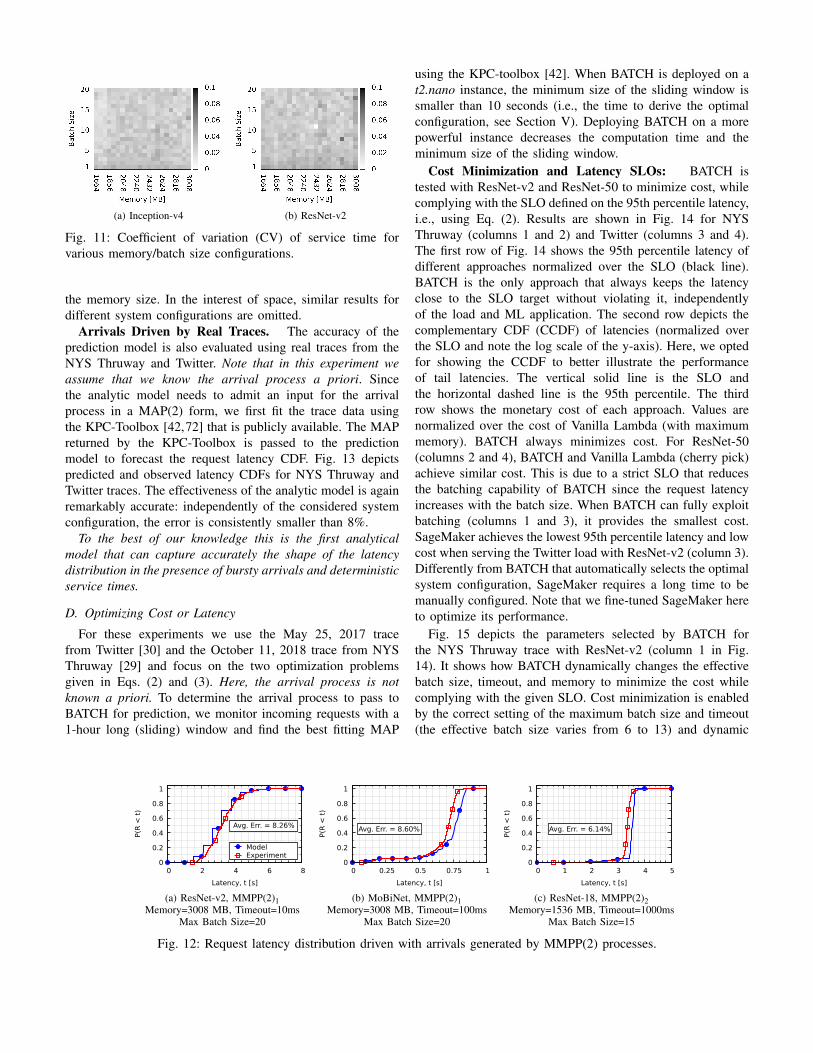
(a) Inception-v4 (b) ResNet-v2
Fig. 11: Coefficient of variation (CV) of service time forvarious memory/batch size configurations.
the memory size. In the interest of space, similar results fordifferent system configurations are omitted.
Arrivals Driven by Real Traces. The accuracy of theprediction model is also evaluated using real traces from theNYS Thruway and Twitter. Note that in this experiment weassume that we know the arrival process a priori. Sincethe analytic model needs to admit an input for the arrivalprocess in a MAP(2) form, we first fit the trace data usingthe KPC-Toolbox [42,72] that is publicly available. The MAPreturned by the KPC-Toolbox is passed to the predictionmodel to forecast the request latency CDF. Fig. 13 depictspredicted and observed latency CDFs for NYS Thruway andTwitter traces. The effectiveness of the analytic model is againremarkably accurate: independently of the considered systemconfiguration, the error is consistently smaller than 8%.
To the best of our knowledge this is the first analyticalmodel that can capture accurately the shape of the latencydistribution in the presence of bursty arrivals and deterministicservice times.
D. Optimizing Cost or Latency
For these experiments we use the May 25, 2017 tracefrom Twitter [30] and the October 11, 2018 trace from NYSThruway [29] and focus on the two optimization problemsgiven in Eqs. (2) and (3). Here, the arrival process is notknown a priori. To determine the arrival process to pass toBATCH for prediction, we monitor incoming requests with a1-hour long (sliding) window and find the best fitting MAP
using the KPC-toolbox [42]. When BATCH is deployed on at2.nano instance, the minimum size of the sliding window issmaller than 10 seconds (i.e., the time to derive the optimalconfiguration, see Section V). Deploying BATCH on a morepowerful instance decreases the computation time and theminimum size of the sliding window.
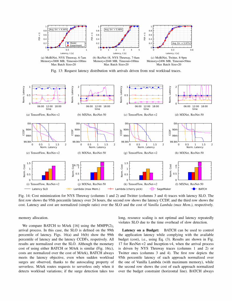
Cost Minimization and Latency SLOs: BATCH istested with ResNet-v2 and ResNet-50 to minimize cost, whilecomplying with the SLO defined on the 95th percentile latency,i.e., using Eq. (2). Results are shown in Fig. 14 for NYSThruway (columns 1 and 2) and Twitter (columns 3 and 4).The first row of Fig. 14 shows the 95th percentile latency ofdifferent approaches normalized over the SLO (black line).BATCH is the only approach that always keeps the latencyclose to the SLO target without violating it, independentlyof the load and ML application. The second row depicts thecomplementary CDF (CCDF) of latencies (normalized overthe SLO and note the log scale of the y-axis). Here, we optedfor showing the CCDF to better illustrate the performanceof tail latencies. The vertical solid line is the SLO andthe horizontal dashed line is the 95th percentile. The thirdrow shows the monetary cost of each approach. Values arenormalized over the cost of Vanilla Lambda (with maximummemory). BATCH always minimizes cost. For ResNet-50(columns 2 and 4), BATCH and Vanilla Lambda (cherry pick)achieve similar cost. This is due to a strict SLO that reducesthe batching capability of BATCH since the request latencyincreases with the batch size. When BATCH can fully exploitbatching (columns 1 and 3), it provides the smallest cost.SageMaker achieves the lowest 95th percentile latency and lowcost when serving the Twitter load with ResNet-v2 (column 3).Differently from BATCH that automatically selects the optimalsystem configuration, SageMaker requires a long time to bemanually configured. Note that we fine-tuned SageMaker hereto optimize its performance.
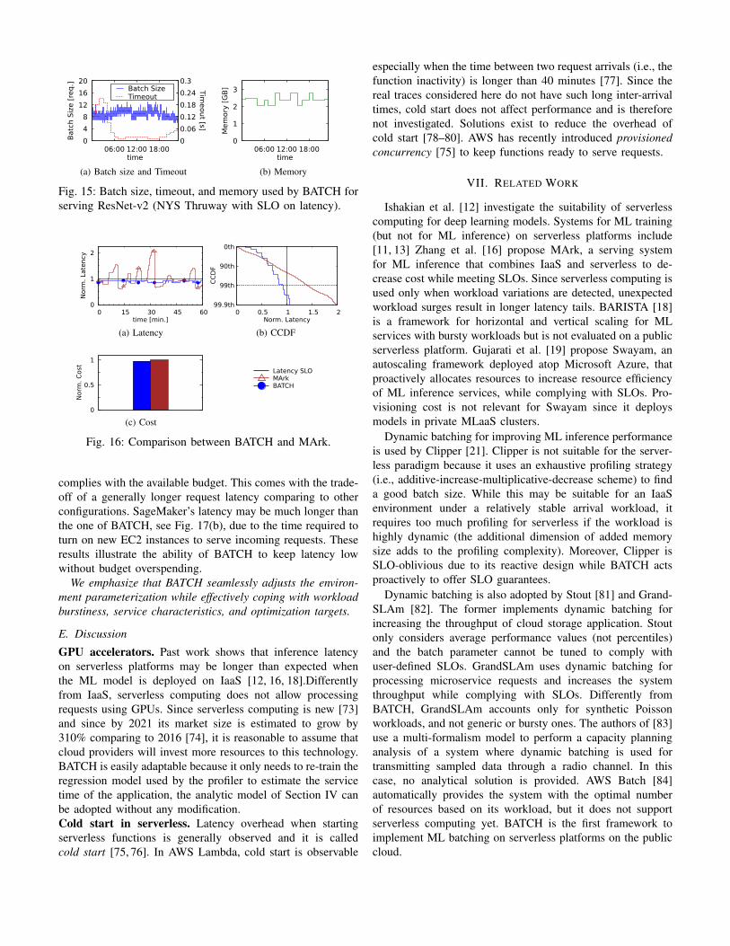
Fig. 15 depicts the parameters selected by BATCH forthe NYS Thruway trace with ResNet-v2 (column 1 in Fig.14). It shows how BATCH dynamically changes the effectivebatch size, timeout, and memory to minimize the cost whilecomplying with the given SLO. Cost minimization is enabledby the correct setting of the maximum batch size and timeout(the effective batch size varies from 6 to 13) and dynamic
0
0.2
0.4
0.6
0.8
1
0 2 4 6 8
Avg. Err. = 8.26%
P(R
< t
)
Latency, t [s]
ModelExperiment
(a) ResNet-v2, MMPP(2)1Memory=3008 MB, Timeout=10ms
Max Batch Size=20
0
0.2
0.4
0.6
0.8
1
0 0.25 0.5 0.75 1
Avg. Err. = 8.60%
P(R
< t
)
Latency, t [s]
(b) MoBiNet, MMPP(2)1Memory=3008 MB, Timeout=100ms
Max Batch Size=20
0
0.2
0.4
0.6
0.8
1
0 1 2 3 4 5
Avg. Err. = 6.14%
P(R
< t
)
Latency, t [s]
(c) ResNet-18, MMPP(2)2Memory=1536 MB, Timeout=1000ms
Max Batch Size=15
Fig. 12: Request latency distribution driven with arrivals generated by MMPP(2) processes.
0
0.2
0.4
0.6
0.8
1
0 0.5 1
Avg. Err. = 4.44%
P(R
< t
)
Latency, t [s]
ModelExperiment
(a) MoBiNet, NYS Thruway, 6-7amMemory=3008 MB, Timeout=100ms
Max Batch Size=20
0
0.2
0.4
0.6
0.8
1
0 1 2 3 4 5
Avg. Err. = 5.48%
P(R
< t
)
Latency, t [s]
(b) ResNet-18, NYS Thruway, 7-8amMemory=2048 MB, Timeout=100ms
Max Batch Size=20
0
0.2
0.4
0.6
0.8
1
0 0.3 0.6
Avg. Err. = 5.97%
P(R
< t
)
Latency, t [s]
(c) MoBiNet, Twitter, 8-9pmMemory=2496 MB, Timeout=50ms
Max Batch Size=20
Fig. 13: Request latency distribution with arrivals driven from real workload traces.
0
0.5
1
06:00 12:00 18:00
Norm
. La
tency
time
(a) TensorFlow, ResNet-v2
0
1
2
06:00 12:00 18:00
Norm
. La
tency
time
(b) MXNet, ResNet-50
0
0.5
1
06:00 12:00 18:00
Norm
. La
tency
time
(c) TensorFlow, ResNet-v2
0
1
2
06:00 12:00 18:00
Norm
. La
tency
time
(d) MXNet, ResNet-50
99.9th
99th
90th
0th
0 0.5 1 1.5 2
CC
DF
Norm. Latency
(e) TensorFlow, ResNet-v2
99.9th
99th
90th
0th
0 0.5 1 1.5 2
CC
DF
Norm. Latency
(f) MXNet, ResNet-50
99.9th
99th
90th
0th
0 0.5 1 1.5 2
CC
DF
Norm. Latency
(g) TensorFlow, ResNet-v2
99.9th
99th
90th
0th
0 0.5 1 1.5 2
CC
DF
Norm. Latency
(h) MXNet, ResNet-50
0
0.5
1
1.5
Norm
. C
ost
(i) TensorFlow, ResNet-v2 0
0.5
1
Norm
. C
ost 6.75
(j) MXNet, ResNet-50 0
0.5
1
1.5
Norm
. C
ost
(k) TensorFlow, ResNet-v2 0
0.5
1N
orm
. C
ost 4
(l) MXNet, ResNet-50
Latency SLO Lambda (max Mem.) Lambda (cherry pick) SageMaker BATCH
Fig. 14: Cost minimization for NYS Thruway (columns 1 and 2) and Twitter (columns 3 and 4) traces with latency SLO. Thefirst row shows the 95th percentile latency over 24 hours, the second row shows the latency CCDF, and the third row shows thecost. Latency and cost are normalized (simple ratio) over the SLO and the cost of Vanilla Lambda (max Mem.), respectively.
memory allocation.
We compare BATCH to MArk [16] using the MMPP(2)1arrival process. In this case, the SLO is defined on the 99thpercentile of latency. Figs. 16(a) and 16(b) show the 99thpercentile of latency and the latency CCDFs, respetively. Allresults are normalized over the SLO. Although the monetarycost of using either BATCH or MArk is similar (Fig. 16(c),costs are normalized over the cost of MArk), BATCH alwaysmeets the latency objective, even when sudden workloadsurges are observed, thanks to the autoscaling property ofserverless. MArk routes requests to serverless only when itdetects workload variations; if the surge detection takes too
long, resource scaling is not optimal and latency repeatedlyviolates SLO due to the time overhead of slow detection.
Latency on a Budget: BATCH can be used to controlthe application latency while complying with the availablebudget (cost), i.e., using Eq. (3). Results are shown in Fig.17 for ResNet-v2 and Inception-v4, when the arrival processis driven by NYS Thruway traces (columns 1 and 2) orTwitter ones (columns 3 and 4). The first row depicts the95th percentile latency of each approach normalized overthe one of Vanilla Lambda (with maximum memory), whilethe second row shows the cost of each approach normalizedover the budget constraint (horizontal line). BATCH always
0
4
8
12
16
20
06:00 12:00 18:00 0
0.06
0.12
0.18
0.24
0.3
Batc
h S
ize [
req
.]
Timeout [s]
time
Batch SizeTimeout
(a) Batch size and Timeout
0
1
2
3
06:00 12:00 18:00
Mem
ory
[G
B]
time
(b) Memory
Fig. 15: Batch size, timeout, and memory used by BATCH forserving ResNet-v2 (NYS Thruway with SLO on latency).
0
1
2
0 15 30 45 60
Norm
. La
tency
time [min.]
(a) Latency
99.9th
99th
90th
0th
0 0.5 1 1.5 2
CC
DF
Norm. Latency
(b) CCDF
0
0.5
1
Norm
. C
ost
(c) Cost
Latency SLOMArkBATCH
Fig. 16: Comparison between BATCH and MArk.
complies with the available budget. This comes with the trade-off of a generally longer request latency comparing to otherconfigurations. SageMaker’s latency may be much longer thanthe one of BATCH, see Fig. 17(b), due to the time required toturn on new EC2 instances to serve incoming requests. Theseresults illustrate the ability of BATCH to keep latency lowwithout budget overspending.
We emphasize that BATCH seamlessly adjusts the environ-ment parameterization while effectively coping with workloadburstiness, service characteristics, and optimization targets.
E. Discussion
GPU accelerators. Past work shows that inference latencyon serverless platforms may be longer than expected whenthe ML model is deployed on IaaS [12, 16, 18].Differentlyfrom IaaS, serverless computing does not allow processingrequests using GPUs. Since serverless computing is new [73]and since by 2021 its market size is estimated to grow by310% comparing to 2016 [74], it is reasonable to assume thatcloud providers will invest more resources to this technology.BATCH is easily adaptable because it only needs to re-train theregression model used by the profiler to estimate the servicetime of the application, the analytic model of Section IV canbe adopted without any modification.Cold start in serverless. Latency overhead when startingserverless functions is generally observed and it is calledcold start [75, 76]. In AWS Lambda, cold start is observable
especially when the time between two request arrivals (i.e., thefunction inactivity) is longer than 40 minutes [77]. Since thereal traces considered here do not have such long inter-arrivaltimes, cold start does not affect performance and is thereforenot investigated. Solutions exist to reduce the overhead ofcold start [78–80]. AWS has recently introduced provisionedconcurrency [75] to keep functions ready to serve requests.
VII. RELATED WORK
Ishakian et al. [12] investigate the suitability of serverlesscomputing for deep learning models. Systems for ML training(but not for ML inference) on serverless platforms include[11, 13] Zhang et al. [16] propose MArk, a serving systemfor ML inference that combines IaaS and serverless to de-crease cost while meeting SLOs. Since serverless computing isused only when workload variations are detected, unexpectedworkload surges result in longer latency tails. BARISTA [18]is a framework for horizontal and vertical scaling for MLservices with bursty workloads but is not evaluated on a publicserverless platform. Gujarati et al. [19] propose Swayam, anautoscaling framework deployed atop Microsoft Azure, thatproactively allocates resources to increase resource efficiencyof ML inference services, while complying with SLOs. Pro-visioning cost is not relevant for Swayam since it deploysmodels in private MLaaS clusters.
Dynamic batching for improving ML inference performanceis used by Clipper [21]. Clipper is not suitable for the server-less paradigm because it uses an exhaustive profiling strategy(i.e., additive-increase-multiplicative-decrease scheme) to finda good batch size. While this may be suitable for an IaaSenvironment under a relatively stable arrival workload, itrequires too much profiling for serverless if the workload ishighly dynamic (the additional dimension of added memorysize adds to the profiling complexity). Moreover, Clipper isSLO-oblivious due to its reactive design while BATCH actsproactively to offer SLO guarantees.
Dynamic batching is also adopted by Stout [81] and Grand-SLAm [82]. The former implements dynamic batching forincreasing the throughput of cloud storage application. Stoutonly considers average performance values (not percentiles)and the batch parameter cannot be tuned to comply withuser-defined SLOs. GrandSLAm uses dynamic batching forprocessing microservice requests and increases the systemthroughput while complying with SLOs. Differently fromBATCH, GrandSLAm accounts only for synthetic Poissonworkloads, and not generic or bursty ones. The authors of [83]use a multi-formalism model to perform a capacity planninganalysis of a system where dynamic batching is used fortransmitting sampled data through a radio channel. In thiscase, no analytical solution is provided. AWS Batch [84]automatically provides the system with the optimal numberof resources based on its workload, but it does not supportserverless computing yet. BATCH is the first framework toimplement ML batching on serverless platforms on the publiccloud.

0
1
2
3
06:00 12:00 18:00
Norm
. La
tency
time
(a) TensorFlow, ResNet-v2
0
5
10
15
06:00 12:00 18:00
Norm
. La
tency
time
(b) TensorFlow, Inception-v4
0
1
2
06:00 12:00 18:00
Norm
. La
tency
time
(c) TensorFlow, ResNet-v2
0
1
2
3
06:00 12:00 18:00
Norm
. La
tency
time
(d) TensorFlow, Inception-v4
0
0.5
1
1.5
2
Norm
. C
ost
(e) TensorFlow, ResNet-v2 0
0.5
1
1.5
2
Norm
. C
ost
(f) TensorFlow, Inception-v4 0
0.5
1
1.5
2
Norm
. C
ost
(g) TensorFlow, ResNet-v2 0
0.5
1
1.5
2
Norm
. C
ost
(h) TensorFlow, Inception-v4
Budget SLO Lambda (max Mem.) Lambda (cherry pick) SageMaker BATCH
Fig. 17: Latency minimization for NYS Thruway (columns 1 and 2) and Twitter (columns 3 and 4) traces with budget SLO. Thefirst row shows the 95th percentile latency over 24 hours and the second row shows the cost. Latency and cost are normalized(simple ratio) over the latency of Vanilla Lambda (max Mem.) and the SLO, respectively.
VIII. CONCLUDING REMARKS
We introduce BATCH, a novel framework for optimiz-ing ML serving on serverless platforms. BATCH uses alightweight profiling strategy and an analytical model toidentify the best parameter configuration (i.e., memory size,batch size, and timeout) to improve the system performancewhile meeting user-defined SLOs. The efficiency of BATCH isevaluated using real traces and comparing its performance withother available strategies (e.g., AWS SageMaker). We showthat BATCH decreases the cost of maintaining the system by50% and can minimize the system performance while meetingthe budget independently of the arrival intensity. Future work-ing includes extending BATCH to support different servicetime distributions and adopting optimization algorithms thatare faster than the exhaustive search used here to support co-optimization of latency and cost.
ACKNOWLEDGEMENT
This work is supported in part by the following grants:National Science Foundation IIS-1838024 (using resourcesprovided by Amazon Web Services as part of the NSF BIG-DATA program), IIS-1838022, CCF-1756013, CCF-1717532,and CNS-1950485. We thank the anonymous reviewers fortheir insightful comments and suggestions that significantlyimproved the paper.
REFERENCES
[1] “Aws lambda – serverless compute,” https://aws.amazon.com/lambda/,[Online; accessed 04-December-2019].
[2] “Ibm cloud – cloud functions,” https://www.ibm.com/cloud/functions/,[Online; accessed 04-December-2019].
[3] “Azure functionsserverless architecture – microsoft azure,” https://azure.microsoft.com/en-us/services/functions/, [Online; accessed 04-December-2019].
[4] “Cloud functions – serverless environment to build and connect cloudservices — google cloud platform,” https://cloud.google.com/functions/,[Online; accessed 04-December-2019].
[5] L. F. Herrera-Quintero, J. C. Vega-Alfonso, K. B. A. Banse, and E. C.Zambrano, “Smart its sensor for the transportation planning based oniot approaches using serverless and microservices architecture,” IEEEIntelligent Transportation Systems Magazine, vol. 10, no. 2, pp. 17–27,2018.
[6] P. Persson and O. Angelsmark, “Kappa: serverless iot deployment,” inProceedings of the 2nd International Workshop on Serverless Comput-ing. ACM, 2017, pp. 16–21.
[7] G. McGrath and P. R. Brenner, “Serverless computing: Design, imple-mentation, and performance,” in 2017 IEEE 37th International Confer-ence on Distributed Computing Systems Workshops (ICDCSW). IEEE,2017, pp. 405–410.
[8] B. Cheng, J. Fuerst, G. Solmaz, and T. Sanada, “Fog function: Serverlessfog computing for data intensive iot services,” in 2019 IEEE Interna-tional Conference on Services Computing (SCC). IEEE, 2019, pp.28–35.
[9] J. Rajewski, “System and method for live streaming content to subscrip-tion audiences using a serverless computing system,” Jun. 7 2018, uSPatent App. 15/369,473.
[10] L. Ao, L. Izhikevich, G. M. Voelker, and G. Porter, “Sprocket: Aserverless video processing framework,” in Proceedings of the ACMSymposium on Cloud Computing. ACM, 2018, pp. 263–274.
[11] J. Carreira, P. Fonseca, A. Tumanov, A. Zhang, and R. Katz, “A casefor serverless machine learning,” in Workshop on Systems for ML andOpen Source Software at NeurIPS, vol. 2018, 2018.
[12] V. Ishakian, V. Muthusamy, and A. Slominski, “Serving deep learningmodels in a serverless platform,” in 2018 IEEE International Conferenceon Cloud Engineering (IC2E). IEEE, 2018, pp. 257–262.
[13] H. Wang, D. Niu, and B. Li, “Distributed machine learning with aserverless architecture,” in IEEE INFOCOM 2019-IEEE Conference onComputer Communications. IEEE, 2019, pp. 1288–1296.
[14] T. Elsken, J. H. Metzen, and F. Hutter, “Neural architecture search: Asurvey.” Journal of Machine Learning Research, vol. 20, no. 55, pp.1–21, 2019.
[15] ——, “Neural architecture search,” in Automated Machine Learning.Springer, 2019, pp. 63–77.
[16] C. Zhang, M. Yu, W. Wang, and F. Yan, “Mark: Exploiting cloud servicesfor cost-effective, slo-aware machine learning inference serving,” in2019 USENIX Annual Technical Conference (USENIX ATC 19), 2019.
[17] J. M. Hellerstein, J. M. Faleiro, J. Gonzalez, J. Schleier-Smith,V. Sreekanti, A. Tumanov, and C. Wu, “Serverless computing: Onestep forward, two steps back,” in CIDR 2019, 9th Biennial Conferenceon Innovative Data Systems Research, Asilomar, CA, USA, January13-16, 2019, Online Proceedings. www.cidrdb.org, 2019. [Online].Available: http://cidrdb.org/cidr2019/papers/p119-hellerstein-cidr19.pdf

[18] A. Bhattacharjee, A. D. Chhokra, Z. Kang, H. Sun, A. Gokhale, andG. Karsai, “Barista: Efficient and scalable serverless serving systemfor deep learning prediction services,” in 2019 IEEE InternationalConference on Cloud Engineering (IC2E). IEEE, 2019, pp. 23–33.
[19] A. Gujarati, S. Elnikety, Y. He, K. S. McKinley, and B. B. Brandenburg,“Swayam: distributed autoscaling to meet slas of machine learninginference services with resource efficiency,” in Proceedings of the 18thACM/IFIP/USENIX Middleware Conference. ACM, 2017, pp. 109–120.
[20] X. Tang, P. Wang, Q. Liu, W. Wang, and J. Han, “Nanily: A qos-aware scheduling for dnn inference workload in clouds,” in 2019IEEE 21st International Conference on High Performance Computingand Communications; IEEE 17th International Conference on SmartCity; IEEE 5th International Conference on Data Science and Systems(HPCC/SmartCity/DSS). IEEE, 2019, pp. 2395–2402.
[21] D. Crankshaw, X. Wang, G. Zhou, M. J. Franklin, J. E. Gonzalez, andI. Stoica, “Clipper: A low-latency online prediction serving system,” in14th USENIX Symposium on Networked Systems Design and Implemen-tation (NSDI 17), 2017, pp. 613–627.
[22] F. Yan, S. Hughes, A. Riska, and E. Smirni, “Overcoming limitationsof off-the-shelf priority schedulers in dynamic environments,” in2013 IEEE 21st International Symposium on Modelling, Analysisand Simulation of Computer and Telecommunication Systems, SanFrancisco, CA, USA, August 14-16, 2013, 2013, pp. 505–514. [Online].Available: https://doi.org/10.1109/MASCOTS.2013.72
[23] N. Mi, A. Riska, E. Smirni, and E. Riedel, “Enhancing dataavailability in disk drives through background activities,” in The38th Annual IEEE/IFIP International Conference on DependableSystems and Networks, DSN 2008, June 24-27, 2008, Anchorage,Alaska, USA, Proceedings, 2008, pp. 492–501. [Online]. Available:https://doi.org/10.1109/DSN.2008.4630120
[24] F. Yan, S. Hughes, A. Riska, and E. Smirni, “Agile middlewarefor scheduling: meeting competing performance requirements ofdiverse tasks,” in ACM/SPEC International Conference on PerformanceEngineering, ICPE’14, Dublin, Ireland, March 22-26, 2014, 2014, pp.185–196. [Online]. Available: https://doi.org/10.1145/2568088.2568104
[25] N. Mi, A. Riska, Q. Zhang, E. Smirni, and E. Riedel, “Efficientmanagement of idleness in storage systems,” ACM Trans. Storage,vol. 5, no. 2, pp. 4:1–4:25, 2009. [Online]. Available: https://doi.org/10.1145/1534912.1534913
[26] M. Abadi, P. Barham, J. Chen, Z. Chen, A. Davis, J. Dean, M. Devin,S. Ghemawat, G. Irving, M. Isard et al., “Tensorflow: A system forlarge-scale machine learning,” in 12th USENIX Symposium on OperatingSystems Design and Implementation (OSDI 16), 2016, pp. 265–283.
[27] G. Neubig, Y. Goldberg, and C. Dyer, “On-the-fly operation batchingin dynamic computation graphs,” in Advances in Neural InformationProcessing Systems, 2017, pp. 3971–3981.
[28] A. Ali, R. Pinciroli, F. Yan, and E. Smirni, “Batch pre-release,” Jun.2020. [Online]. Available: https://doi.org/10.5281/zenodo.3872213
[29] “Nys thruway origin and destination points for all vehicles,”https://data.ny.gov/Transportation/NYS-Thruway-Origin-and-Destination-Points-for-All-/em4e-ui5w, [Online; accessed 14-November-2019].
[30] ArchiveTeam, “Twitter streaming traces, 2017.”[31] “Amazon. build, train, and deploy machine learning models at scale.”
https://docs.aws.amazon.com/lambda/latest/dg/resource-model.html,[Online; accessed 03-December-2019].
[32] M. Arlitt and T. Jin, “A workload characterization study of the 1998world cup web site,” IEEE network, vol. 14, no. 3, pp. 30–37, 2000.
[33] A. Riska and E. Riedel, “Disk drive level workload characterization,”in Proceedings of the 2006 USENIX Annual Technical Conference,Boston, MA, USA, May 30 - June 3, 2006, 2006, pp. 97–102. [Online].Available: http://www.usenix.org/events/usenix06/tech/riska.html
[34] N. Mi, G. Casale, L. Cherkasova, and E. Smirni, “Injecting realisticburstiness to a traditional client-server benchmark,” in Proceedings ofthe 6th international conference on Autonomic computing. ACM, 2009,pp. 149–158.
[35] J. Xue, R. Birke, L. Y. Chen, and E. Smirni, “Managing data centertickets: Prediction and active sizing,” in 2016 46th Annual IEEE/IFIPInternational Conference on Dependable Systems and Networks (DSN).IEEE, 2016, pp. 335–346.
[36] N. Mi, Q. Zhang, A. Riska, E. Smirni, and E. Riedel, “Performanceimpacts of autocorrelated flows in multi-tiered systems,” Perform.Evaluation, vol. 64, no. 9-12, pp. 1082–1101, 2007. [Online].Available: https://doi.org/10.1016/j.peva.2007.06.016
[37] N. Mi, G. Casale, L. Cherkasova, and E. Smirni, “Burstiness inmulti-tier applications: Symptoms, causes, and new models,” inMiddleware 2008, ACM/IFIP/USENIX 9th International MiddlewareConference, Leuven, Belgium, December 1-5, 2008, Proceedings, ser.Lecture Notes in Computer Science, V. Issarny and R. E. Schantz,Eds., vol. 5346. Springer, 2008, pp. 265–286. [Online]. Available:https://doi.org/10.1007/978-3-540-89856-6\ 14
[38] “Aws autoscaling,” https://aws.amazon.com/autoscaling, [Online; ac-cessed 03-December-2019].
[39] “Aws lambda – pricing,” https://aws.amazon.com/lambda/pricing/, [On-line; accessed 30-October-2019].
[40] S. Xu, H. Zhang, G. Neubig, W. Dai, J. K. Kim, Z. Deng, Q. Ho,G. Yang, and E. P. Xing, “Cavs: An efficient runtime system for dy-namic neural networks,” in 2018 USENIX Annual Technical Conference(USENIX ATC 18), 2018, pp. 937–950.
[41] “Make data useful,” http://www.scribd.com/doc/4970486/Make-Data-Useful-by-Greg-Linden-Amazoncom, [Online; accessed 15-January-2020].
[42] G. Casale, E. Z. Zhang, and E. Smirni, “Kpc-toolbox: Best recipes forautomatic trace fitting using markovian arrival processes,” PerformanceEvaluation, vol. 67, no. 9, pp. 873–896, 2010.
[43] M. F. Neuts, “A versatile markovian point process,” Journal of AppliedProbability, vol. 16, no. 4, pp. 764–779, 1979.
[44] P. Royston and W. Sauerbrei, Multivariable model-building: a pragmaticapproach to regression anaylsis based on fractional polynomials formodelling continuous variables. John Wiley & Sons, 2008, vol. 777.
[45] F. Yan, O. Ruwase, Y. He, and E. Smirni, “Serf: efficient scheduling forfast deep neural network serving via judicious parallelism,” in SC’16:Proceedings of the International Conference for High PerformanceComputing, Networking, Storage and Analysis. IEEE, 2016, pp. 300–311.
[46] T. Zhu, A. Tumanov, M. A. Kozuch, M. Harchol-Balter, and G. R.Ganger, “Prioritymeister: Tail latency qos for shared networked storage,”in Proceedings of the ACM Symposium on Cloud Computing. ACM,2014, pp. 1–14.
[47] N. Li, H. Jiang, D. Feng, and Z. Shi, “Pslo: enforcing the x th percentilelatency and throughput slos for consolidated vm storage,” in Proceedingsof the Eleventh European Conference on Computer Systems. ACM,2016, p. 28.
[48] L. Kleinrock, Queueing systems. Volume I: theory. wiley New York,1975.
[49] F. Yan, Y. He, O. Ruwase, and E. Smirni, “Efficient deep neuralnetwork serving: Fast and furious,” IEEE Trans. Network and ServiceManagement, vol. 15, no. 1, pp. 112–126, 2018. [Online]. Available:https://doi.org/10.1109/TNSM.2018.2808352
[50] G. Casale, N. Mi, and E. Smirni, “Model-driven system capacityplanning under workload burstiness,” IEEE Transactions on Computers,vol. 59, no. 1, pp. 66–80, 2009.
[51] A. Reibman and K. Trivedi, “Numerical transient analysis of markovmodels,” Computers & Operations Research, vol. 15, no. 1, pp. 19–36,1988.
[52] W. Fischer and K. Meier-Hellstern, “The markov-modulated poissonprocess (mmpp) cookbook,” Performance evaluation, vol. 18, no. 2, pp.149–171, 1993.
[53] J. Bernardo, M. Bayarri, J. Berger, A. Dawid, D. Heckerman, A. Smith,and M. West, “The markov modulated poisson process and markovpoisson cascade with applications to web traffic modeling,” BayesianStatistics, 2003.
[54] N. Bean, D. Green, and P. Taylor, “The output process of an mmpp/m/1queue,” Journal of Applied Probability, vol. 35, no. 4, pp. 998–1002,1998.
[55] X. Lu, J. Yin, H. Chen, and X. Zhao, “An approach for bursty andself-similar workload generation,” in International Conference on WebInformation Systems Engineering. Springer, 2013, pp. 347–360.
[56] F. Bause, P. Buchholz, and J. Kriege, “A comparison of markovian arrivaland arma/arta processes for the modeling of correlated input processes,”in Proceedings of the 2009 Winter Simulation Conference (WSC). IEEE,2009, pp. 634–645.
[57] G. Casale, E. Z. Zhang, and E. Smirni, “Trace data characterization andfitting for markov modeling,” Perform. Evaluation, vol. 67, no. 2, pp. 61–79, 2010. [Online]. Available: https://doi.org/10.1016/j.peva.2009.09.003
[58] M. F. Neuts, Structured stochastic matrices of M/G/1 type and theirapplications. Marcel Dekker New York, 1989, vol. 5.

[59] A. Riska and E. Smirni, “Mamsolver: A matrix analytic methodstool,” in Computer Performance Evaluation, Modelling Techniquesand Tools 12th International Conference, TOOLS 2002, London, UK,April 14-17, 2002, Proceedings, ser. Lecture Notes in ComputerScience, T. Field, P. G. Harrison, J. T. Bradley, and U. Harder,Eds., vol. 2324. Springer, 2002, pp. 205–211. [Online]. Available:https://doi.org/10.1007/3-540-46029-2\ 14
[60] G. Casale, N. Mi, L. Cherkasova, and E. Smirni, “How to parameter-ize models with bursty workloads,” ACM SIGMETRICS PerformanceEvaluation Review, vol. 36, no. 2, pp. 38–44, 2008.
[61] “Lambda package documentation,” https://aws.amazon.com/premiumsupport/knowledge-center/build-python-lambda-deployment-package/, [Online; accessed 19-June-2019].
[62] T. Chen, M. Li, Y. Li, M. Lin, N. Wang, M. Wang, T. Xiao, B. Xu,C. Zhang, and Z. Zhang, “Mxnet: A flexible and efficient machinelearning library for heterogeneous distributed systems,” arXiv preprintarXiv:1512.01274, 2015.
[63] “Boto 3 documentation,” https://boto3.amazonaws.com/v1/documentation/api/latest/index.html, [Online; accessed 19-December-2019].
[64] “Aws cloudwatch,” https://aws.amazon.com/cloudwatch/, [Online; ac-cessed 04-April-2020].
[65] “Amazon ec2 t2 instances,” https://aws.amazon.com/ec2/instance-types/t2/, [Online; accessed 7-January-2020].
[66] “Aws kinesis,” https://aws.amazon.com/kinesis/?nc=sn&loc=0, [Online;accessed 04-April-2020].
[67] O. Russakovsky, J. Deng, H. Su, J. Krause, S. Satheesh, S. Ma,Z. Huang, A. Karpathy, A. Khosla, M. Bernstein et al., “Imagenet largescale visual recognition challenge,” International journal of computervision, vol. 115, no. 3, pp. 211–252, 2015.
[68] H. Phan, D. Huynh, Y. He, M. Savvides, and Z. Shen, “Mobinet:A mobile binary network for image classification,” arXiv preprintarXiv:1907.12629, 2019.
[69] K. He, X. Zhang, S. Ren, and J. Sun, “Deep residual learning for imagerecognition,” in Proceedings of the IEEE conference on computer visionand pattern recognition, 2016, pp. 770–778.
[70] C. Szegedy, S. Ioffe, V. Vanhoucke, and A. A. Alemi, “Inception-v4,inception-resnet and the impact of residual connections on learning,” inThirty-First AAAI Conference on Artificial Intelligence, 2017.
[71] “Load testing for production variant automatic scaling,”https://github.com/awsdocs/amazon-sagemaker-developer-guide/blob/master/doc source/endpoint-scaling-loadtest.md, [Online; accessed07-January-2020].
[72] G. Casale, E. Z. Zhang, and E. Smirni, “Kpc-toolbox: Simpleyet effective trace fitting using markovian arrival processes,” inFifth International Conference on the Quantitative Evaluaiton ofSystems (QEST 2008), 14-17 September 2008, Saint-Malo, France.
IEEE Computer Society, 2008, pp. 83–92. [Online]. Available:https://doi.org/10.1109/QEST.2008.33
[73] P. Castro, V. Ishakian, V. Muthusamy, and A. Slominski, “The riseof serverless computing,” Commun. ACM, vol. 62, no. 12, pp. 44–54,2019. [Online]. Available: http://doi.acm.org/10.1145/3368454
[74] Businesswire, “$7.72 billion function-as-a-service market 2017 - globalforecast to 2021: Increasing shift from devops to serverless computingto drive the overall function-as-a-service market - research and markets,”https://www.businesswire.com/news/home/20170227006262/en/7.72-Billion-Funct\%20ion-as-a-Service-Market-2017---Global, [Online;accessed 16-December-2019].
[75] “New for aws lambda – predictable start-up times with provisionedconcurrency,” https://aws.amazon.com/blogs/compute/new-for-aws-lambda-predictable-start-up-times-with-provisioned-concurrency/,[Online; accessed 9-January-2020].
[76] L. Wang, M. Li, Y. Zhang, T. Ristenpart, and M. Swift, “Peeking behindthe curtains of serverless platforms,” in 2018 USENIX Annual TechnicalConference (USENIX ATC 18), 2018, pp. 133–146.
[77] W. Lloyd, S. Ramesh, S. Chinthalapati, L. Ly, and S. Pallickara,“Serverless computing: An investigation of factors influencing microser-vice performance,” in 2018 IEEE International Conference on CloudEngineering (IC2E). IEEE, 2018, pp. 159–169.
[78] E. Oakes, L. Yang, D. Zhou, K. Houck, T. Harter, A. Arpaci-Dusseau,and R. Arpaci-Dusseau, “Sock: Rapid task provisioning with serverless-optimized containers,” in 2018 USENIX Annual Technical Conference(USENIX ATC 18), 2018, pp. 57–70.
[79] A. Mohan, H. Sane, K. Doshi, S. Edupuganti, N. Nayak, and V. Sukhom-linov, “Agile cold starts for scalable serverless,” in 11th USENIXWorkshop on Hot Topics in Cloud Computing (HotCloud 19), 2019.
[80] K. Mahajan, S. Mahajan, V. Misra, and D. Rubenstein, “Exploitingcontent similarity to address cold start in container deployments,” in Pro-ceedings of the 15th International Conference on emerging NetworkingEXperiments and Technologies, 2019, pp. 37–39.
[81] J. C. McCullough, J. Dunagan, A. Wolman, and A. C. Snoeren, “Stout:An adaptive interface to scalable cloud storage,” in Proc. of the USENIXAnnual Technical Conference–ATC, 2010, pp. 47–60.
[82] R. S. Kannan, L. Subramanian, A. Raju, J. Ahn, J. Mars, and L. Tang,“Grandslam: Guaranteeing slas for jobs in microservices executionframeworks,” in Proceedings of the Fourteenth EuroSys Conference2019, 2019, pp. 1–16.
[83] R. Pinciroli, M. Gribaudo, M. Roveri, and G. Serazzi, “Capacityplanning of fog computing infrastructures for smart monitoring,” inWorkshop on New Frontiers in Quantitative Methods in Informatics.Springer, 2017, pp. 72–81.
[84] “Aws batch,” https://aws.amazon.com/batch/, [Online; accessed 13-January-2020].

Appendix: Artifact Description/Artifact Evaluation
SUMMARY OF THE EXPERIMENTS REPORTEDWe prototype batch atop AWS lambda and conducted the exper-iments using two machine learning frameworks Tensorflow andMxNet. We use 4 popular computer vision applications (ResNet18,ResNet52, MoBiNet, Inception-V4, and ResNet-V2) to demonstratethe adaptability of BATCH. A theoretical MMPP arrival process,Traffic of the NYS Thruway traces and Twitter traces as our real-world traces are used as a workload. BATCH uses Boto 3 to enablecommunication with the serverless platform. Every time a newoptimal memory size is identified by the performance optimizer,BATCH invokes a low-level API to update the function configura-tion (i.e., the memory allocated to the function). In order to predictthe workload intensity, We used the KPC toolbox. All the perfor-mance logs i.e. billing time and latency are collected through AWScloud watch with default settings. We deploy our model on lambdausing the TensorFlow version 1.8.
ARTIFACT AVAILABILITYSoftware Artifact Availability: Some author-created software ar-
tifacts are NOT maintained in a public repository or are NOT avail-able under an OSI-approved license.
Hardware Artifact Availability: There are no author-created hard-ware artifacts.
Data Artifact Availability: There are no author-created dataartifacts.
Proprietary Artifacts: None of the associated artifacts, author-created or otherwise, are proprietary.
Author-Created or Modified Artifacts:
Persistent ID: http://doi.org/10.5281/zenodo.3872213,
https://github.com/rickypinci/BATCH.git↪→
Artifact name: BATCH
BASELINE EXPERIMENTAL SETUP, ANDMODIFICATIONS MADE FOR THE PAPER
Relevant hardware details: t2micro(Ec2 instance), AWS Lambda,AWS cloud watch
Operating systems and versions: Ubutnu
Applications and versions: ResNet18, ResNet52, MoBiNet,Inception-V4, and ResNet-V2
Libraries and versions: BOTO3, Tensorflow 1.8, MxNet modelserver
Key algorithms: Computer Vision
Input datasets and versions: ImageNet-22K dataset
URL to output from scripts that gathers execution environmentinformation.https://github.com/rickypinci/BATCH/blob/master/outp ⌋
ut.log↪→
ARTIFACT EVALUATIONVerification and validation studies: We performed the verification
and validation studies on AWS lambda using Tensorflow andMxNetmodel server. As theoretical arrival processes, MMPP arrivals, andas real arrival trace, we use Traffic of the NYS Thruway and Twittertraces for validating BATCH. Serving requests are extracted fromthe ImageNet-22K dataset. Popular computer vision ML modelssuch as ResNet18, ResNet52, MoBiNet, Inception-V4, and ResNet-V2 are deployed on Lambda to demonstrate the adaptability ofBATCH for different application sizes and complexities.
Accuracy and precision of timings: All the measured values areextracted from the AWS cloud watch and the precision of the tim-ing values in up to milliseconds. We use the default cloudwatchconfiguration for the collection of logs. BATCH generates threedifferent logs (Lambda logs, Batch logs, and Request logs) files aftercollecting the logs from cloudwatch. Lambda logs provide detailedinformation of excitation for each invocation i.e. initialization time,container id, execution time, memory utilization, memory allocated,and billing time. Batch logs provide the information related to eachbatch i.e. batch arrival time, batch departure time, and batch size.Finally, the request logs provide details of each request such asrequest arrival time, response time and departure time.
Used manufactured solutions or spectral properties: We used AWSlambda as our main serverless cloud service. Tensorflow 1.8 andMxNet model server is used as a machine learning API. varioussizes of computer vision ML models as our serving applicationdeployed on AWS Lambda.
Quantified the sensitivity of results to initial conditions and/or pa-rameters of the computational environment: Overall the performanceresults are collected through AWS cloud watch and each experimentis conducted long enough to generate stable results(minimum dura-tion 1 hour). During our experiments, we observed the behavior ofAWS lambda to be stable for varying parameters such as memorysize, batch size, and batch timeout.
Controls, statistics, or other steps taken to make the measurementsand analyses robust to variability and unknowns in the system. Allthe results are collected through amazon’s built-in logging mecha-nism for the cost (billing time) as well as performance. However,during the experiments, we do not take into consideration the net-work overhead. We take into consideration pure computation timeand queuing time (time each request spent in the buffer).