bayes estimator for coefficient of variation and inverse ... · harvey and merwe (2012) make a...

International Journal of Statistics and Systems

ISSN 0973-2675 Volume 12, Number 4 (2017), pp. 721-732

© Research India Publications

http://www.ripublication.com

Bayes Estimator for Coefficient of Variation and

Inverse Coefficient of Variation for the Normal

Distribution

Aruna Kalkur T.

St.Aloysius College (Autonomous) Mangaluru, Karnataka India.

Aruna Rao

Professor (Retd.)

Mangalore University, Karnataka, India

Abstract

In this paper Bayes estimators of Coefficient of Variation (CV) and Inverse

Coefficient of Variation (ICV) of a normal distribution are derived using five

objective priors namely Left invariant, Right invariant, Jeffry’s Rule prior,

Uniform prior and Probability matching prior. Mean Square Error (MSE) of

these estimators are derived to the order of 𝑂(1𝑛⁄ ) and the expressions are new.

Numerical results indicate that Maximum Likelihood Estimators (MLE) of CV

and ICV have smaller MSE compared to Bayes estimators. It is further shown

that in a certain class of estimators MLE of CV and ICV are not admissible.

Key words: Bayes estimators, Objective priors, Mean Square Error,

Admissibility.

1. Introduction

The estimation and confidence interval for Coefficient of Variation (CV) of a normal

distribution is well addressed in the literature. The original work dates back to 1932

when Mckay derived a confidence interval for the CV of a normal distribution using

transformed CV. (Also see the references cited in this paper).

It was Singh (1983) who emphasized that Inverse Sample Coefficient of Variation

722 Aruna Kalkur T. and Aruna Rao

(ISCV) can be used to derive confidence interval for the CV of a distribution. He

derived the first four moments of the ISCV. Sharma and Krishnan (1994) developed

the asymptotic distribution of the ISCV without making an assumption about the

population distribution.

Although many papers have appeared for the estimation and the confidence interval of

a normal distribution, they are derived using the classical theory of inference. In recent

years Bayesian inference is widely used in scientific investigation. When objective

priors are used the Bayes estimator performs well compared to the classical estimator

in terms of mean square error. Not many papers have appeared in the past regarding

Bayes estimator of CV of the normal distribution.

In this paper, we discuss Bayes estimator for of the CV and ICV of the normal

distribution under squared error loss function. We have used objective priors so that the

bias and Mean Square Error (MSE) of these estimators can be compared with maximum

likelihood estimators. The objective priors used are Left invariant, Right invariant,

Jeffry’s Rule prior, Uniform prior and Probability matching prior.

In Chapter 1 we have listed many papers dealing with the estimation for the CV of the

normal distribution. In this chapter, we discuss Bayes estimator for the CV and ICV of

the normal distribution under squared error loss function. We have used objective priors

so that the bias and MSE of these estimators can be compared with MLEs. The objective

priors used are Right invariant, Left invariant, Jeffrey’s Rule prior, Uniform prior and

Probability matching prior.

Harvey and Merwe (2012) make a distinction between Jeffrey’s prior and Jeffry’s Rule

prior. Both are proportional to square root of the determinant of the Fisher Information

matrix; but the distinction is that in Jeffrey’s prior σ is treated as parameter and in

Jeffrey’s Rule prior σ2 is treated as parameter. The comparison between the Bayes

estimator, maximum likelihood and other estimators of the classical inference are the

focal point of investigation in many research papers in the past. Some of the research

references are the following:

Pereira and Stern (2000) derived Full Bayesian Test for the CV of the normal

distribution. Kang and Kim (2003) proposed Bayesian test procedure for the equality

of CVs of two normal distributions using fractional Bayes factor. Pang et al. (2005)

derived Bayesian credible intervals for the CVs of three parameters Lognormal and

Weibull distributions. D’Cunha and Rao (2014) compared Bayesian credible interval

and confidence interval based on MLE in lognormal distribution.

This chapter is divided into 6 sections. Section 2 presents the expressions for the Bayes

estimators of CV using five objective priors mentioned previously. The bias and MSE

of the Bayes estimator of CV to the order of 𝑂(1)and𝑂(1𝑛⁄ ) respectively are also

derived. Numerical values of bias and MSE of the Bayes estimator for CVs, along with

the MLE’s are presented in section 3. In section 4 we present the expressions for the

Bayes Estimator for Coefficient of Variation and Inverse Coefficient… 723

Bayes estimator of ICV along with the bias and MSE to the order of 𝑂(1)and𝑂(1𝑛⁄ )

respectively. Numerical values of bias and MSE of the Bayes estimator for ICV, along

with the MLE’s are presented in section 5. The chapter concludes in section 6.

2. Bayes Estimators of Coefficient of Variation

Let 𝑥1, … , 𝑥𝑛 be i.i.d. N (μ, σ2). The maximum likelihood estimator of CV of the normal

distribution is given by𝜃 =�̂�

�̂�, where �̂� = �̅� =

1

𝑛∑ 𝑥𝑖

𝑛𝑖=1 and �̂�2=𝑠2 =

1

𝑛−1∑ (𝑛

𝑖=1 𝑥𝑖 −

�̅�)2 denotes the sample mean and sample variance of normal distribution respectively.

Five priors are used for the estimation of CV and ICV. Let 𝜋(𝜇, 𝜎) denote the prior

density for μ and σ. The expressions for the prior density are given below.

a) Right invariant Jeffrey’s prior

𝜋(𝜇, 𝜎) =1

𝜎 (1)

b) Left invariant prior

𝜋(𝜇, 𝜎) = 1

𝜎2 (2)

c) Jeffrey’s Rule prior

𝜋(𝜇, 𝜎 ) = 1

𝜎3 (3)

d) Uniform prior

𝜋(𝜇, 𝜎 ) = 1 (4)

e) Probability matching prior

𝜋(𝜇, 𝜎) = 𝜎2 (5)

Since the distribution of �̅� and 𝑠2 are independent, after some simplification we obtain

the posterior density of (1

𝜎2) as Gamma ((𝑛+2

2) ,

1

2(𝑛 − 1)𝑠2) under right invariant

prior, Gamma ((𝑛+3

2) ,

1

2(𝑛 − 1)𝑠2) under left invariant Jeffreys prior,


Gamma((𝑛+4

2) ,

1

2(𝑛 − 1)𝑠2) under Jeffry’s Rule prior, Gamma ((

𝑛+1

2) ,

1

2(𝑛 − 1)𝑠2)

under Uniform prior and Gamma ((𝑛

2) ,

1

2(𝑛 − 1)𝑠2) under Probability matching prior.

Bayes estimator of CV is given by 𝐸(𝜎

𝜇 ), where the expectation is taken with respect to

the posterior density of 𝜋(𝜇 , 𝜎|𝑑𝑎𝑡𝑎).

The posterior density 𝝅(𝝁, 𝝈|𝒙𝟏 , … , 𝒙𝒏 ) for the right invariant, left invariant, Jeffrey’s

Rule, Uniform and Probability matching priors respectively are given by the following

expressions.

𝜋(𝜇, 𝜎|𝑥1, … , 𝑥𝑛)

=1

√2𝜋𝜎

√𝑛

𝑒−

12

(�̅�−𝜇)2

𝜎2𝑛⁄

((𝑛 − 1)𝑠2

2 )

𝑛+22

Γ (𝑛 + 2

2 )(

1

𝜎2)

(𝑛+2

2)−1

𝑒−

12

(𝑛−1𝜎2 )𝑠2

,

(Using Right invariant prior) −∞ < 𝜇 < ∞, 𝜎 > 0

(6)

𝜋(𝜇, 𝜎|𝑥1, … , 𝑥𝑛) =1

√2𝜋𝜎

√𝑛

𝑒−

1

2

(�̅�−𝜇)2

𝜎2𝑛⁄

((𝑛−1)𝑠2

2)

𝑛+32

Γ(𝑛+3

2)

(1

𝜎2)(

𝑛+3

2)−1

𝑒−

1

2(

𝑛−1

𝜎2 )𝑠2

, (7)

(Using Left invariant prior) −∞ < 𝜇 < ∞, 𝜎 > 0

𝜋(𝜇, 𝜎|𝑥1, … , 𝑥𝑛) =1

√2𝜋𝜎

√𝑛

𝑒−

1

2

(�̅�−𝜇)2

𝜎2𝑛⁄

((𝑛−1)𝑠2

2)

𝑛+42

Γ(𝑛+4

2)

(1

𝜎2)

(𝑛+4

2)−1

𝑒−

1

2(

𝑛−1

𝜎2 )𝑠2

, (8)

(Using Jeffrey’s Rule prior) −∞ < 𝜇 < ∞, 𝜎 > 0

𝜋(𝜇, 𝜎|𝑥1, … , 𝑥𝑛) =1

√2𝜋𝜎

√𝑛

𝑒−

1

2

(�̅�−𝜇)2

𝜎2𝑛⁄

((𝑛−1)𝑠2

2)

𝑛+12

Γ(𝑛+1

2)

(1

𝜎2)(

𝑛+1

2)−1

𝑒−

1

2(

𝑛−1

𝜎2 )𝑠2

, (9)

(Using Uniform prior) −∞ < 𝜇 < ∞, 𝜎 > 0

𝜋(𝜇, 𝜎|𝑥1, … , 𝑥𝑛) =1

√2𝜋𝜎

√𝑛

𝑒−

1

2

(�̅�−𝜇)2

𝜎2𝑛⁄

((𝑛−1)𝑠2

2)

𝑛2

Γ(𝑛

2)

(1

𝜎2)(

𝑛

2)−1

𝑒−

1

2(

𝑛−1

𝜎2 )𝑠2

, (10)

(Using Probability matching prior) −∞ < 𝜇 < ∞, 𝜎 > 0


The Bayes estimator of CV is 𝐸(𝜃|𝑥1, … , 𝑥𝑛 ), where the expectation is taken with

respect to the posterior density of 𝜇 and 𝜎. For the right invariant prior it is given by

𝜃𝑅 = ∬𝜇

𝜎

1

√2𝜋𝜎

√𝑛

𝑒−

1

2

(�̅�−𝜇)2

𝜎2𝑛⁄

((𝑛−1)𝑠2

2)

𝑛+22

Γ(𝑛+2

2)

(1

𝜎2)(

𝑛+2

2)−1

𝑒−

1

2(

𝑛−1

𝜎2 )𝑠2

𝑑𝜇𝑑𝜎 (11)

= Г(

𝑛+2

2)(

𝑛−1

2)

1/2(

𝑠

�̅�)

Г(𝑛+3

2)

= 𝑎𝑛𝜃 , where𝑎𝑛 = Г(

𝑛+2

2)(

𝑛−1

2)

1/2

Г(𝑛+3

2)

and 𝜃=(𝑠

�̅�) (12)

The following theorem gives the Bayes estimators.

Theorem 1: The Bayes estimators of CV corresponding to Left Invariant prior, Right

Invariant prior, Jeffrey’s Rule prior, Uniform prior and Probability Matching prior are

the following.

𝜃𝑅 = Г(

𝑛+2

2)(

𝑛−1

2)

1/2(

𝑠

�̅�)

Г(𝑛+3

2)

(13)

𝜃𝐿=Г(

𝑛+1

2)(

𝑛−1

2)

1/2(

𝑠

�̅�)

Г(𝑛+2

2)

(14)

𝜃JR = Г(

𝑛+3

2)(

𝑛−1

2)

1/2(

𝑠

�̅�)

Г(𝑛+4

2)

(15)

𝜃U = (Г(

𝑛

2))(

𝑛−1

2)

1/2(

𝑠

�̅�)

Г(𝑛+1

2)

(16)

and 𝜃PM = (Г(

𝑛−1

2))(

𝑛−1

2)

1/2(

𝑠

�̅�)

Г(𝑛

2)

respectively. (17)

Proof: Straight forward and is omitted.


3. Bias and Mean Square Error of the Bayes Estimators of Coefficient of Variation

Theorem 2: The following table gives the bias and mean square error to the order

𝑂(1) and 𝑂(1𝑛⁄ ) for different estimators of CV.

Prior Bias MSE

1. Right

Invariant Г(

𝑛+2

2)(

𝑛−1

2)

1/2(

𝑠

�̅�)

Г(𝑛+3

2)

– (𝜎

𝜇)

(𝑠

�̅�)

4

𝑛+

(𝑠

�̅�)

2

2𝑛+(

Г(𝑛+2

2)(

𝑛−1

2)

1/2(

𝑠

�̅�)

Г(𝑛+3

2)

− (𝜎

𝜇))2

2. Left

Invariant Г(

𝑛+1

2)(

𝑛−1

2)

1/2(

𝑠

�̅�)

Г(𝑛+2

2)

–(𝜎

𝜇)

(𝑠

�̅�)

4

𝑛+

(𝑠

�̅�)

2

2𝑛+(

(Г(𝑛+1

2)(

𝑛−1

2)

12(

𝑠

�̅�)

Г(𝑛+3

2)

− (𝜎

𝜇))2

3. Jeffrey’s

Rule Г(

𝑛+3

2)(

𝑛−1

2)

1/2(

𝑠

�̅�)

Г(𝑛+4

2)

– (𝜎

𝜇)

(𝑠

�̅�)

4

𝑛+

(𝑠

�̅�)

2

2𝑛+(

(Г(𝑛+3

2)(

𝑛−1

2)

12(

𝑠

�̅�)

Г(𝑛+4

2)

− (𝜎

𝜇))2

4. Uniform Г(𝑛

2)(

𝑛−1

2)

1/2(

𝑠

�̅�)

Г(𝑛+1

2)

– (𝜎

𝜇)

(𝑠

�̅�)

4

𝑛+

(𝑠

�̅�)

2

2𝑛+(

(Г(𝑛

2)(

𝑛−1

2)

12(

𝑠

�̅�)

Г(𝑛+1

2)

− (𝜎

𝜇))2

5. Probability

Matching Г(

𝑛−1

2)(

𝑛−1

2)

1/2(

𝑠

�̅�)

Г(𝑛

2)

– (𝜎

𝜇)

(𝑠

�̅�)

4

𝑛+

(𝑠

�̅�)

2

2𝑛+(

(Г(𝑛−1

2)(

𝑛−1

2)

12(

𝑠

�̅�)

Г(𝑛

2)

− (𝜎

𝜇))2

Proof: Given in the Appendix.

Consider the class of estimators {𝑎 �̂�}. This class includes the MLE �̂� as well as various

Bayes estimators for different choice of an. The following theorem gives the optimal

estimator in this class.

Theorem 3: Among the class of estimators {𝑎 �̂�} of Coefficient of variation 𝜃, where

�̂� denotes the maximum likelihood estimator of 𝜃, the estimator with minimum mean

square error to the order of 𝑂(1𝑛⁄ ) is

�̂�

(1

𝑛)(�̂�2+1)+1

Proof: The expression for MSE of (a �̂�) is given by

MSE of (𝑎𝜃) =𝑎2V(𝜃) + Bias of (a𝜃)2 (17)

=𝑎2V(𝜃) +(𝜃2(𝑎-1) 2

Differentiating with respect to 𝑎 and equating it with zero we get

a=1

(1

𝑛)(𝜃2+1)+1

(18)


Substituting 𝜃 for 𝜃 in a we get estimator as �̂�

(1

𝑛)(�̂�2+1)+1

, this is the optimal estimator

in the class of 𝑎𝜃. As n→ ∞,�̂�

(1

𝑛)(�̂�2+1)+1

→ �̂�

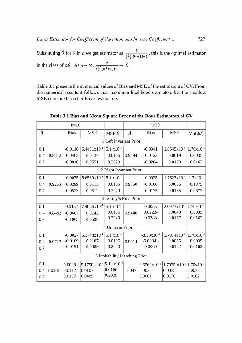
Table 3.1 presents the numerical values of Bias and MSE of the estimators of CV. From

the numerical results it follows that maximum likelihood estimators has the smallest

MSE compared to other Bayes estimators.

Table 3.1 Bias and Mean Square Error of the Bays Estimators of CV

n=10 n=30

θ Bias MSE MSE(𝜃) 𝐴𝑛 Bias MSE MSE(𝜃)

1.Left Invariant Prior

0.1

0.4

0.7

0.8842

-0.0116

-0.0463

-0.0810

6.4401x10-4

0.0127

0.0551

5.1 x10-4

0.0106

0.2020

0.9594

-0.0041

-0.0122

-0.0284

1.8645x10-4

0.0019

0.0170

1.70x10-4

0.0035

0.0162

2.Right Invariant Prior

0.1

0.4

0.7

0.9253

-0.0075

-0.0299

-0.0523

5.6580x10-4

0.0115

0.0512

5.1 x10-4

0.0106

0.2020

0.9750

-0.0025

-0.0100

-0.0175

1.7623x10-4

0.0036

0.0165

1.7x10-4

0.1375

0.0673

3.Jeffrey’s Rule Prior

0.1

0.4

0.7

0.8482

0.0152

-0.0607

-0.1063

7.4046x10-4

0.0142

0.0598

5.1 x10-4

0.0106

0.2020 0.9446

-0.0055-

0.0222-

0.0388

2.0073x10-4

0.0040

0.0177

1.70x10-4

0.0035

0.0162

4.Uniform Prior

0.1

0.4

0.7

0.9727

-0.0027

-0.0109

-0.0191

5.1748x10-4

0.0107

0.0489

5.1 x10-4

0.0106

0.2020 0.9914

-8.58x10-4

-0.0034 -

0.0060

1.7074x10-4

0.0035

0.0162

1.70x10-4

0.0035

0.0162

5.Probability Matching Prior

0.1

0.4

0.7

1.0281

0.0028

0.0112

0.0197

5.1790 x10-4

0.0107

0.0489

5.1 x10-4

0.0106

0.2020 1.0087

8.6562x10-4

0.0035

0.0061

1.7075 x10-4

0.0035

0.0170

1.70x10-4

0.0035

0.0162


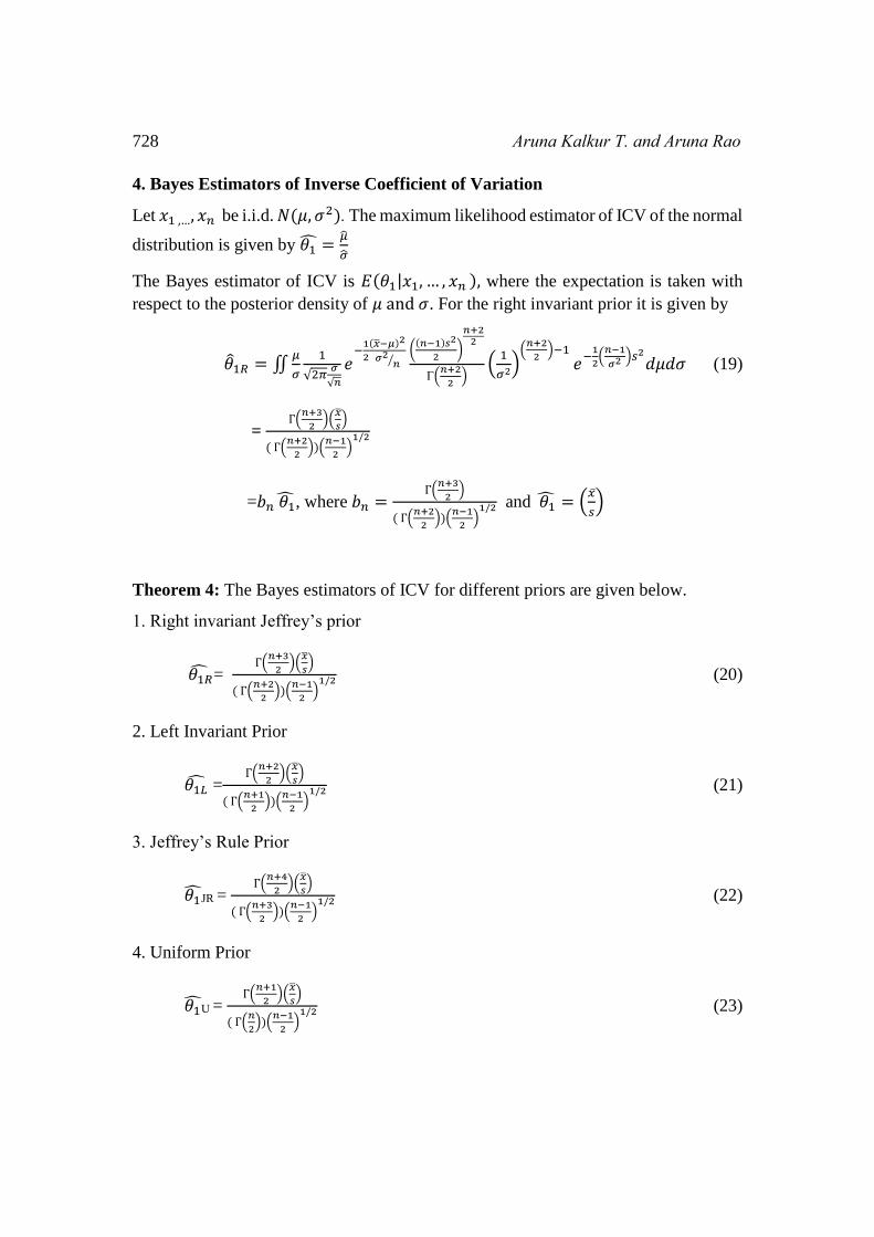
4. Bayes Estimators of Inverse Coefficient of Variation

Let 𝑥1 ,…, 𝑥𝑛 be i.i.d. 𝑁(𝜇, 𝜎2). The maximum likelihood estimator of ICV of the normal

distribution is given by 𝜃1̂ =�̂�

�̂�

The Bayes estimator of ICV is 𝐸(𝜃1|𝑥1, … , 𝑥𝑛 ), where the expectation is taken with

respect to the posterior density of 𝜇 and 𝜎. For the right invariant prior it is given by

𝜃1𝑅 = ∬𝜇

𝜎

1

√2𝜋𝜎

√𝑛

𝑒−

1

2

(�̅�−𝜇)2

𝜎2𝑛⁄

((𝑛−1)𝑠2

2)

𝑛+22

Γ(𝑛+2

2)

(1

𝜎2)(

𝑛+2

2)−1

𝑒−

1

2(

𝑛−1

𝜎2 )𝑠2

𝑑𝜇𝑑𝜎 (19)

= Г(

𝑛+3

2)(

�̅�

𝑠)

( Г(𝑛+2

2))(

𝑛−1

2)

1/2

=𝑏𝑛 𝜃1̂, where 𝑏𝑛 =Г(

𝑛+3

2)

( Г(𝑛+2

2))(

𝑛−1

2)

1/2 and 𝜃1̂ = (�̅�

𝑠)

Theorem 4: The Bayes estimators of ICV for different priors are given below.

1. Right invariant Jeffrey’s prior

𝜃1�̂�= Г(

𝑛+3

2)(

�̅�

𝑠)

( Г(𝑛+2

2))(

𝑛−1

2)

1/2 (20)

2. Left Invariant Prior

𝜃1�̂� =Г(

𝑛+2

2)(

�̅�

𝑠)

( Г(𝑛+1

2))(

𝑛−1

2)

1/2 (21)

3. Jeffrey’s Rule Prior

𝜃1̂JR = Г(

𝑛+4

2)(

�̅�

𝑠)

( Г(𝑛+3

2))(

𝑛−1

2)

1/2 (22)

4. Uniform Prior

𝜃1̂U = Г(

𝑛+1

2)(

�̅�

𝑠)

( Г(𝑛

2))(

𝑛−1

2)

1/2 (23)


5. Probability Matching Prior

𝜃1̂PM = Г(

𝑛

2)(

�̅�

𝑠)

( Г(𝑛−1

2))(

𝑛−1

2)

1/2 (24)

Proof: Straight forward and is omitted.

5. Bias and Mean Square Error of the Bayes Estimator of Inverse Coefficient of

Variation

Theorem 5: The following table gives the bias and mean square error to the order

𝑂(1)and𝑂(1𝑛⁄ ) respectively of different estimators of ICV.

Prior Bias MSE

1. Right Invariant Г(𝑛+3

2)(

�̅�

𝑠)

( Г(𝑛+2

2))(

𝑛−1

2)

1/2 - (𝜇

𝜎) 1

𝑛+

(�̅�

𝑠)

2

2𝑛+(

Г(𝑛+3

2)(

�̅�

𝑠)

( Г(𝑛+2

2))(

𝑛−1

2)

1/2 − (𝜇

𝜎))2

2. Left Invariant Г(𝑛+2

2)(

�̅�

𝑠)

( Г(𝑛+1

2))(

𝑛−1

2)

1/2 -(𝜇

𝜎) 1

𝑛+

(�̅�

𝑠)

2

2𝑛+(

Г(𝑛+2

2)(

�̅�

𝑠)

( Г(𝑛+1

2))(

𝑛−1

2)

1/2 − (𝜇

𝜎))2

3. Jeffrey’s Rule Г(𝑛+4

2)(

�̅�

𝑠)

( Г(𝑛+3

2))(

𝑛−1

2)

1/2-(𝜇

𝜎) 1

𝑛+

(�̅�

𝑠)

2

2𝑛+(

Г(𝑛+4

2)(

�̅�

𝑠)

( Г(𝑛+3

2))(

𝑛−1

2)

1/2 − (𝜇

𝜎))2

4. Uniform Г(𝑛+1

2)(

�̅�

𝑠)

( Г(𝑛

2))(

𝑛−1

2)

1/2-(𝜇

𝜎) 1

𝑛+

(�̅�

𝑠)

2

2𝑛+(

Г(𝑛+1

2)(

�̅�

𝑠)

( Г(𝑛

2))(

𝑛−1

2)

1/2 − (𝜇

𝜎))2

5. Probability Matching Г(𝑛

2)(

�̅�

𝑠)

( Г(𝑛−1

2))(

𝑛−1

2)

1/2-(𝜇

𝜎) 1

𝑛+

(�̅�

𝑠)

2

2𝑛+(

Г(𝑛

2)(

�̅�

𝑠)

( Г(𝑛−1

2))(

𝑛−1

2)

1/2 − (𝜇

𝜎))2

Proof: Given in the Appendix.

Theorem 6: Among the class of estimators {𝑏 �̂�1} of Inverse Coefficient of

variation 𝜃1, where �̂�1 denotes the maximum likelihood estimator of 𝜃1, the estimator

with minimum mean square error to the order of 𝑂(1𝑛⁄ ) is

𝜃1̂

(1

𝑛)(

1

�̂�12+

1

2)+1

Proof: The expression for MSE of (b𝜃1̂) is given by

MSE of (b𝜃1̂) =𝑏2𝑉(𝜃1̂) +𝜃12(𝑏-1)2 (25)


Differentiating with respect to b and equating it to zero we get

b= 𝜃1

2

𝑉(𝜃1)+𝜃12 =

1

(1

𝑛)(

1

𝜃12+

1

2)+1

(26)

Substituting �̂�1 for 𝜃1 in b we get estimator as 𝜃1̂

(1

𝑛)(

1

�̂�12+

1

2)+1

, which is the optimal

estimator.

As n→ ∞, 𝑏𝜃1̂ → 𝜃1̂

Table 5.1 presents the numerical values of Bias and MSE of the estimators of ICV.

From the numerical results it follows that maximum likelihood estimators have the

smallest MSE compared to other Bayes estimators.

Table 5.1. Bias and Mean Square Error of the Bays Estimators of ICV

n=10 n=30

θ1 𝐵𝑛 Bias MSE MSE(𝜃1̂) 𝐵𝑛 Bias MSE MSE(𝜃1)̂

1.Left Invariant Prior

0.1

0.4

0.7

1.1309

0.0131

0.0524

0.0916

5.1002

0.4152

0.2104

5.1000

0.4125

0.0485

1.0423 0.0042

0.0169

0.0296

1.7000

0.1378

0.0682

1.7000

0.1375

0.0673

2.Right Invariant Prior

0.1

0.4

0.7

1.0807

0.0081

0.0323

0.0565

5.1001

0.4135

0.2052

5.1000

0.4125

0.0485

1.0256

0.0026

0.0102

0.0179

1.7000

0.1376

0.0677

1.7000

0.1375

0.0673

3.Jeffrey’s Rule Prior

0.1

0.4

0.7

1.1790

0.0179

0.0716

0.1253

5.1003

0.4176

0.2177

5.1000

0.4125

0.0485

1.0587

0.0059

0.0235

0.0411

1.7000

0.1381

0.0690

1.7000

0.1375

0.0673

4.Uniform Prior 4.

0.1

0.4

0.7

1.0281

0.0028

0.0112

0.0197

5.1000

0.4126

0.2024

5.1000

0.4125

0.0485

1.0087

8.656x10-4

0.0035

0.0061

1.7000

0.1375

0.0674

1.7000

0.1375

0.0673

5.Probability Matching Prior

0.1

0.4

0.7

0.9727

-0.0027

-0.0109

-0.0191

5.1000

0.4126

0.2024

5.1000

0.4125

0.0485

0.9914

8.582x10-4

0.0034

0.0060

1.7000

0.1375

0.0674

1.7000

0.1375

0.0673


6. Conclusion

In this chapter we derive five Bayes estimators of coefficients of variation (CV) as well

as Inverse Coefficient of Variation (ICV) respectively. The bias and mean square error

(MSE) of these estimators are derived to the order of 𝑂(1) and 𝑂(1𝑛⁄ ) respectively.

The numerical results indicate that the maximum likelihood estimator (MLE) of CV

and ICV has smaller MSE compared to the Bayes estimators of CV and ICV. Among

the class of estimators {𝑎𝜃} of CV, the MLE 𝜃 of CV is dominated by the estimator

�̂�

(1

𝑛)(�̂�2+1)+1

to the order of 𝑂(1𝑛⁄ ). In a parallel result the MLE of �̂�1 of ICV is

dominated by the estimator 𝜃1̂

(1

𝑛)(

1

�̂�12+

1

2)+1

to the order of 𝑂(1𝑛⁄ ).

APPENDIX

Proof of Theorem 3:

Using right invariant prior, the bias of Bayes estimator of CV is given by

𝐵𝑖𝑎𝑠(𝜃, 𝜃)= 𝐸(𝜃) − 𝜃)

∬𝜎

𝜇

1

√2𝜋𝜎

√𝑛

𝑒−

1

2

(�̅�−𝜇)2

𝜎2𝑛⁄

((𝑛−1)𝑠2

2)

𝑛+22

Γ(𝑛+2

2)

(1

𝜎2)(

𝑛+2

2)−1

𝑒−

1

2(

𝑛−1

𝜎2 )𝑠2

𝑑𝜇𝑑𝜎 - 𝜎

𝜇 =

Г(𝑛+2

2)(

𝑛−1

2)

1/2

Г(𝑛+3

2)

−𝜎

𝜇

The MSE (𝜃) = 𝐸((𝜃 − 𝜃)2

) =𝑉(𝜃) + 𝐵𝑖𝑎𝑠(𝜃, 𝜃)2

The MSE of 𝜃 using right invariant prior is given by

MSE (𝜃) =1

𝑛𝜃4 +

1

2𝑛𝜃2+(∬

𝜇

𝜎

1

√2𝜋𝜎

√𝑛

𝑒−

1

2

(�̅�−𝜇)2

𝜎2𝑛⁄

((𝑛−1)𝑠2

2)

𝑛+22

Γ(𝑛+2

2)

(1

𝜎2)

(𝑛+2

2)−1

𝑒−

1

2(

𝑛−1

𝜎2 )𝑠2

𝑑𝜇𝑑𝜎 − 𝜎

𝜇)2

=1

𝑛𝜃4 +

1

2𝑛𝜃2+(

Г(𝑛+2

2)(

𝑛−1

2)

1/2(

𝜎

�̅�)

Г(𝑛+3

2)

− 𝜃)2 , where 𝜃 =𝜎

𝜇.


Proof of Theorem 5

Using right invariant prior the bias of Bayes estimator of ICV is given by

∬𝜇

𝜎

1

√2𝜋𝜎

√𝑛

𝑒−

1

2

(�̅�−𝜇)2

𝜎2𝑛⁄

((𝑛−1)𝑠2

2)

𝑛+22

Γ(𝑛+2

2)

(1

𝜎2)(

𝑛+2

2)−1

𝑒−

1

2(

𝑛−1

𝜎2 )𝑥2

𝑑𝜇𝑑𝜎 - 𝜇

𝜎 =

Г(𝑛+3

2)(

�̅�

�̅�)

( Г(𝑛+2

2))(

𝑛−1

2)

1/2 − 𝜇

𝜎

The MSE of 𝜃1 using right invariant prior is given by

1

𝑛+

1

2𝑛𝜃1

2 + (∬𝜇

𝜎

1

√2𝜋𝜎

√𝑛

𝑒−

1

2

(�̅�−𝜇)2

𝜎2𝑛⁄

((𝑛−1)𝑠2

2)

𝑛+22

Γ(𝑛+2

2)

(1

𝜎2)(

𝑛+2

2)−1

𝑒−

1

2(

𝑛−1

𝜎2 )𝑥2

𝑑𝜇𝑑𝜎 − 𝜃1)2 =1

𝑛+

1

2𝑛𝜃1

2+(Г(

𝑛+3

2)(

�̅�

𝑠)

( Г(𝑛+2

2))(

𝑛−1

2)

1/2 - 𝜃1)2, where 𝜃1 = 𝜇

𝜎

Similarly the Bias and MSEs of other Bayes estimators of CV and ICV can be obtained.

References

[1] D‘Cunha, J.G., &Rao, K.A. (2015). Application of Bayesian inference for the

analysis of stock prices. Advances and Applications in Statistics, 6 (1), 57-78.

[2] Harvey, J., & Van der Merwe, A. J. (2012). Bayesian confidence Intervals for

Means and Variances of Lognormal and Bivariate lognormal distributions.

Journal of Statistical Planning and Inference, 142(6), 1294-1309.

[3] McKay, A.T. (1932). Distribution of the Co-efficient of variation and the

extended‘t’ distribution. Journal of Royal Statistics Society.95, 696-698. [4] Pang W.K., Leung P.K., Huang W. K. and W. Liu. (2003). On Bayesian

Estimation of the coefficient of variation for three parameter Weibull,

Lognormal and Gamma distributions.

[5] Pereira, C.A.B., Stern J.M. (1999b). Evidence and Credibility: Full Bayesian

Significance Test for Precise Hypothesis, Entropy 1, 69-80.

[6] Singh M. (1993). Behavior of Sample Coefficient of Variation drawn from

several distributions, Sankya, 55, series B., Pt 1, 65-76.

[7] Sharma and Krishna (1994). Asymptotic sampling distribution of inverse

coefficient of variation and its applications. IEEE Transactions on Reliability.

43(4), 630-633.

bayes estimator for coefficient of variation and inverse ... · harvey and merwe (2012) make a...

Documents