bayesian approach for inverse problem in microwave tomography_jpiof2008ver2.pdf · bayesian...

Bayesian Approach for Inverse Problem in Microwave Tomography

Hacheme Ayasso

Ali Mohammad-Djafari Bernard Duchene

Laboratoire des Signaux et Systemes, UMRS 08506 (CNRS-SUPELEC-UNIV PARIS SUD 11),3 rue Joliot-Curie, F-91192 Gif-sur-Yvette cedex, France

Journees Problemes Inverses et Optimisation de Forme17 - 18 decembre 2008

Introduction

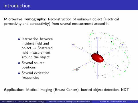
Microwave Tomography: Reconstruction of unknown object (electricalpermetivity and conductivity) from several measurement around it.

Interaction betweenincident field andobject → Scatteredfield measurementaround the object

Several sourcepositions

Several excitationfrequencies

Einc

y

z

x

D

S

Application: Medical imaging (Breast Cancer), burried object detection, NDT

H.AYASSO & al. (LSS(CNRS-SUPELEC-UPS)) Bayesian Microwave Tomography Reconstruction Nantes, 17-18 Decemeber 2008 2 / 23

General Context

Forward Model

~E scat = S (χ)

~E scat : scatter field measurement around the object (data)

χ : unknown object (contrast function) under test

S : system transfere function (Forward Model).

Difficulties

1 Calculating χ given ~E scat & S → An ill-posed inverse problem (Hadamard).

2 S is non-linear.

3 High computational cost.

Proposed Method1 Bayesian inference framework with Gauss-Markov Potts priors

2 Joint source contrast estimation

3 Careful choice of calculation methods & parallel programing


Outline

1 Forward ModelFormulationDifficultiesGradiant-FFT methodsValidation

2 Bayesian Inversion ApproachFormulationPrior ModelIterative LinearizationJoint estimation

3 Conclusion

4 References


1. Forward Model


Forward Formulation(Continuous)

Using the integral equation representation for electrical field

~E scat(~r) =

(1 +

1

k20

~∇~r ~∇~r)∫

D

G(~r ,~r ′)χ(~r ′)~E (~r ′)d~r ′, ~r ∈ S

~E (~r) = ~E inc(~r) +

(1 +

1

k20

~∇~r ~∇~r)∫

D

G(~r ,~r ′)χ(~r ′)~E (~r ′)d~r ′, ~r ∈ D

χ(~r) = ω2ε0µ0εr (r) + iωµ0σ(r)~E (~r),~r ∈ D: total field in thedomain of interest D~E scat ,~r ∈ S : scatter field inmeasuement domain SFoward problem: χ, ~E inc → ~E scat ,Inverse problem: ~E scat , ~E inc → χ Einc

y

z

x

D

S


Forward Formulation(Discretization)

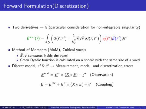
Two derivatives → G (particular consideration for non-integrable singularity)

~E scat(~r) =

∫D

(G(~r ,~r ′) +

1

k20

~∇~r ~∇~rG(~r ,~r ′)

)χ(~r ′)~E (~r ′)d~r ′

Method of Moments (MoM), Cubical voxels~E , χ constants inside the voxelGreen Dyadic function is calculated on a sphere with the same size of a voxel

Discret model, εc & εo → Measurement, model, and discretization errors

E scat = G o × (X ◦ E ) + εo (Observation)

E = E inc + G c × (X ◦ E ) + εc (Coupling)


Difficulties

1 Nonlinear forward model → calculate E

E scat = G o ×(

X ◦(I − G c • XT

)−1

× Einc

)+ ε

2 A =(I − G c • XT

)Large full complex matrix

Memory problem.E = A−1E inc High computational cost

Solution: “Gradiant-FFT” Method

Cost Min required(One frequency!)voxel per axe n 64X 2× n3 × Nf ≈ 0.5Me = 1.5MB

E ou E inc N = 6× n3 × Nf ≈ 1.5Me = 12MBG c ou A 18× n6 × Nf ≈ 1.2Te = 10TBGE (Mem/Cal) O(N2)/O(N3) 10TB/0.5EmCG (Mem/Cal) O(N)/O(K × N2) 12MB/K × 10TmCG-FFT O(N)/O(K × N log(N)) 12MB/10Mm


Gradiant-FFT methods

Solve large complex linear system

E inc =(E − G c × (X ◦ E )

)= A (E )

G c × (X ◦ E )⇔ Discret Convolution product → G o is diagonal in Fourierdomain (Need for zero padding ”circularity”)

Forward operator

A (E ) = E − FT−1(FT (G c)× FT (X ◦ E )

)Adjoint operator

A† (E ) = E − X ∗ ◦ FT−1(FT (G c)× FT (E )

)BiCGSTAB-FFT [Xu2002] High convergence speed compared to classsicalCG-FFTs method


Validation

Comparaison with scattered field real data.

Amplitude


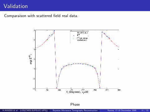
Validation

Comparaison with scattered field real data.

Phase


2.Bayesian Inversion Approach


Prior ModelPrior information: objects are composed of a finite number of homogeneousmaterials

Hidden field representing materials z

Homogeneity within a class → p(X |z) ∼ N (µz , vz)




Spatial dependency between hidden field sites → Potts prior p(z)

Independent prior for X |z → Mixture of Independent Gaussians (MIG)




Spatial dependency between hidden field sites → Potts prior p(z)

Gauss markov prior for X |z → Mixture of Gauss-Markov (MGM)


Hierarchical Model

Partialy unsupervised approach → Estimation of most of the model hyperparameterObject

MIG : p(X (r)|z(r) = k,mk , vk) = N (mk , vk)MGM : p(X (r)|z(r),mk , vk , f (r ′), z(r ′), r ′ ∈ V(r)) = N (µz(r), vz(r))

Hidden field

p(z |γ) ∝ exphP

r∈R Φ(z(r))

+ 12γ

Pr∈R

Pr′∈V(r) δ(z(r)− z(r ′))

iHyper-parameters:

p(mk |m0, v0) = N (m0, v0), ∀kp(v−1

k |a0, b0) = G(a0, b0), ∀kp(α|α0) = D(α0, · · · , α0)p(v−1

ε |ae0 , be0 ) = G(ae0 , be0 )

Constants(Hyper-hyperparameter):m0, v0, a0, b0, α0, ae0 , be0 , γ

X

zk

αk

mkvk

m0 , v0

α0

S + +

0v

a0 ,b0 ae0 ,be0

Escat


Iterative Linearization

Nonlinear Forward model → Estimate the total field E in alternance with thecontrast X and other model parameters.

Algorithm

1 Initial guess for total field E = E inc (Born approximation) and Modelparameter

2 E itr−1, z itr−1, θitr−1 -MAP

X itr (A linear inverse problem)

p(X itr |E itr−1, Escat, z itr−1, θitr−1) ∝ p(E scat |X itr , E itr−1, z itr−1, θitr−1)p(X |E itr−1, z itr−1, θitr−1)

3 X itr -Forward Model

E itr

4 X itr -MAP

z itr , θitr (segmentation problem)

p(z itr , θitr |X itr ) ∝ p(X itr |z itr , θitr )p(z itr , θitr )


Alternated Estimation (Application 1)

MIG prior with independent hidden field sites:Sphere

(a) BIM (Real Part) (b) BIM (imaginary Part)

(c) Bayesian(Real Part) (d) Bayesian (Imaginary Part)


Alternated Estimation (Application 2)

Two spheres:

(a) BIM (Real Part) (b) BIM (imaginary Part)

(c) Bayesian(Real Part) (d) Bayesian (Imaginary Part)


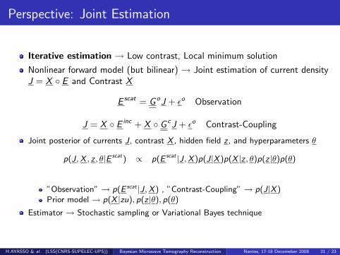
Perspective: Joint Estimation

Iterative estimation → Low contrast, Local minimum solution

Nonlinear forward model (but bilinear) → Joint estimation of current densityJ = X ◦ E and Contrast X

E scat = G oJ + εo Observation

J = X ◦ E inc + X ◦ G cJ + εo Contrast-Coupling

Joint posterior of currents J, contrast X , hidden field z , and hyperparameters θ

p(J,X , z , θ|E scat) ∝ p(E scat |J,X )p(J|X )p(X |z , θ)p(z |θ)p(θ)

”Observation” → p(E scat |J,X ) , ”Contrast-Coupling” → p(J|X )Prior model → p(X |zu), p(z |θ), p(θ)

Estimator → Stochastic sampling or Variational Bayes technique


Conclusion

Microwave Tomography: Nonlinear ill-posed inverse problem with highcomputational cost.

BiCGSTAB-FFT method for forward problem.

Bayesian framework for inverse problem.

Hierarchical mixture model to account for the knowmedge of number ofmaterials and piecewise homogeneity prior information.

Iterative estimation: better results than conventional methods

Perspective:

Joint estimation of current density, contrast, hidden field, and hyperparametersApplication of Variational Bayes approximation technique for the posterior


References

H. Ayasso, B. Duchene, A. Mohammad-Djafari,“A Bayesian approach to microwave

imaging in a 3-D configuration”,in OIPE, 2008.

O. Feron, B. Duchene, A. Mohammad-Djafari, ”Microwave imaging of

inhomogeneous objects made of a finite number of dielectric and conductive

materials from experimental data”, Inverse Problems, vol. 21, no. 6, 2005, pp.

S95–S115.

O. Feron, B. Duchene, A. Mohammad-Djafari, ”Microwave imaging of piecewise

constant objects in a 2D-TE configuration”, Int. J. Appl. Electromagn. Mechan.,

vol. 26, 2007, pp. 167–174.

X. Xu, Q.H. Liu, et Z.W. Zhang, “The stabilized biconjugate gradient fast Fourier

transform method for electromagnetic scattering,” Antennas and Propagation

Society International Symposium, 2002. IEEE, vol. 2, 2002.

H. Ayasso, A. Mohammad-Djafari, ”Variational Bayes With Gauss-Markov-Potts

Prior Models For Joint Image Restoration And Segmentation”, in VISSAP, 2008.


bayesian approach for inverse problem in microwave tomography_jpiof2008ver2.pdf · bayesian...

Documents