bayesian approaches to cognitive sciences. word learning bayesian property induction theory-based...
TRANSCRIPT
Bayesian approaches to cognitive sciences
• Word learning
• Bayesian property induction
• Theory-based causal inference
Word Learning
Word Learning
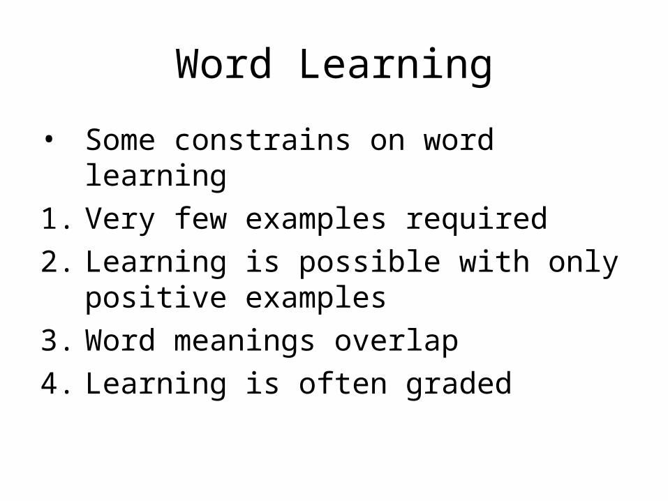
• Some constrains on word learning
1. Very few examples required
2. Learning is possible with only positive examples
3. Word meanings overlap
4. Learning is often graded
Word Learning
• Given a few instances of a particular words, say ‘dog’, how do we generalize to new instance?
• Hypothesis elimination: use deductive logic (along with prior knowledge) to eliminate hypothesis that are inconsistent with the use of the word.
Word Learning
• Some constrains on word learning
1. Very few examples required
2. Learning is possible with only positive examples
3. Word meaning overlap
4. Learning is often graded
Word Learning
• Given a few instances of a particular words, say ‘dog’, how do we generalize to new instance?
• Connectionist (associative) approach: compute the probability of co-occurrences of object features and the corresponding word

Word Learning
• Some constrains on word learning
1. Very few examples required
2. Learning is possible with only positive examples
3. Word meaning overlap
4. Learning is often graded
Word learning
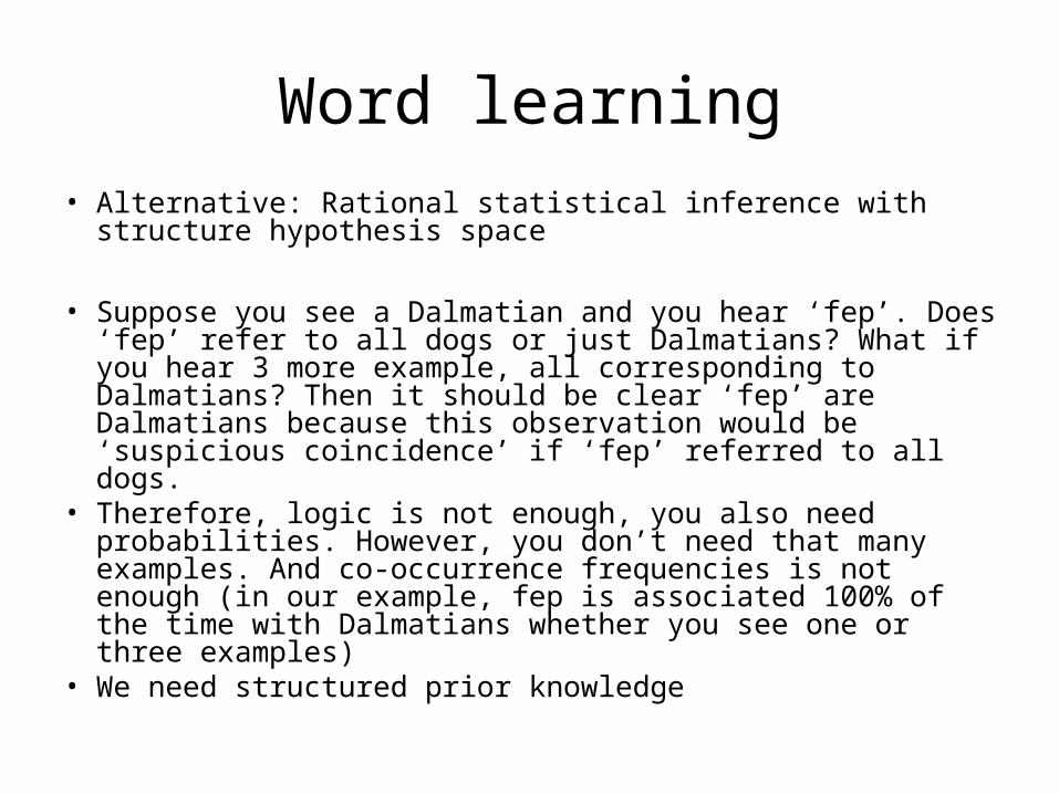
• Alternative: Rational statistical inference with structure hypothesis space
• Suppose you see a Dalmatian and you hear ‘fep’. Does ‘fep’ refer to all dogs or just Dalmatians? What if you hear 3 more example, all corresponding to Dalmatians? Then it should be clear ‘fep’ are Dalmatians because this observation would be ‘suspicious coincidence’ if ‘fep’ referred to all dogs.
• Therefore, logic is not enough, you also need probabilities. However, you don’t need that many examples. And co-occurrence frequencies is not enough (in our example, fep is associated 100% of the time with Dalmatians whether you see one or three examples)
• We need structured prior knowledge
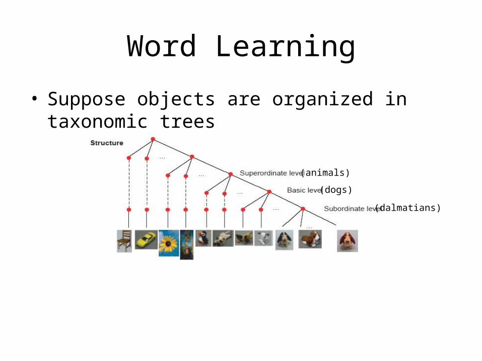
Word Learning
• Suppose objects are organized in taxonomic trees
(animals)
(dogs)
(dalmatians)
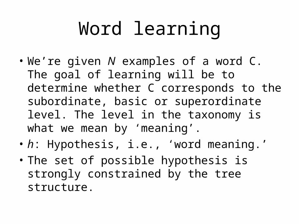
Word learning
• We’re given N examples of a word C. The goal of learning will be to determine whether C corresponds to the subordinate, basic or superordinate level. The level in the taxonomy is what we mean by ‘meaning’.
• h: Hypothesis, i.e., ‘word meaning.’
• The set of possible hypothesis is strongly constrained by the tree structure.
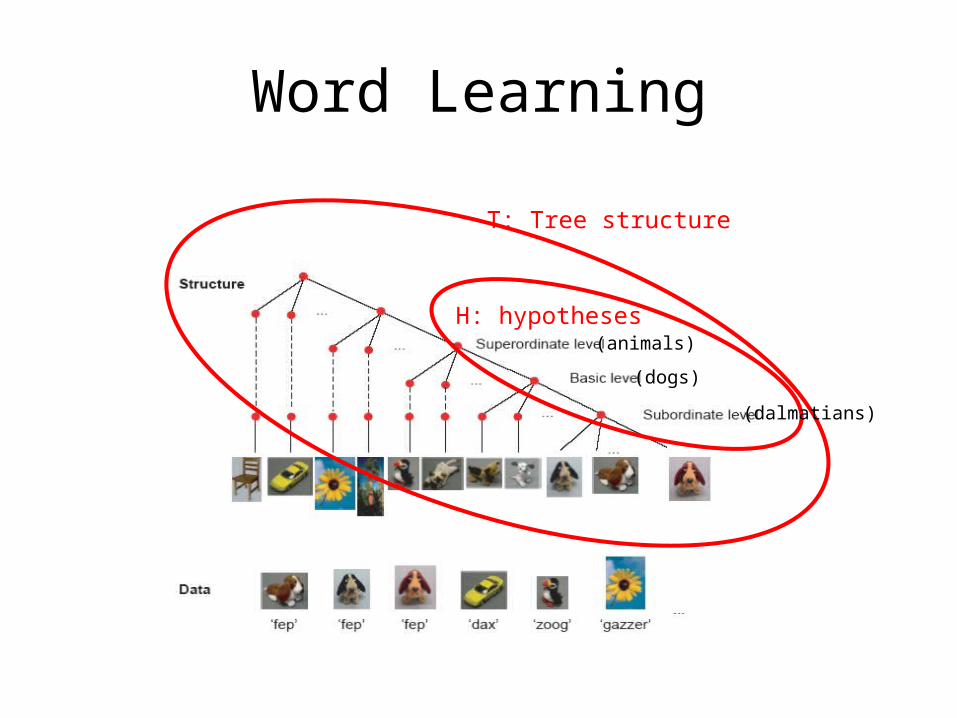
Word Learning
H: hypotheses
T: Tree structure
(animals)
(dogs)
(dalmatians)
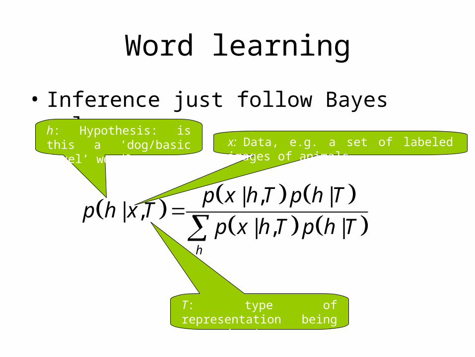
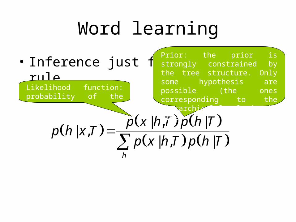
Word learning
• Inference just follow Bayes rule
| , |
| ,| , |
h
p x h T p h Tp h x T
p x h T p h T
h: Hypothesis: is this a ‘dog/basic level’ word?
T: type of representation being assumed (e.g. tree stucture)
x: Data, e.g. a set of labeled images of animals
Word learning
• Inference just follow Bayes rule
| , |
| ,| , |
h
p x h T p h Tp h x T
p x h T p h T
Likelihood function: probability of the data
Prior: the prior is strongly constrained by the tree structure. Only some hypothesis are possible (the ones corresponding to the hierarchical levels in the tree)
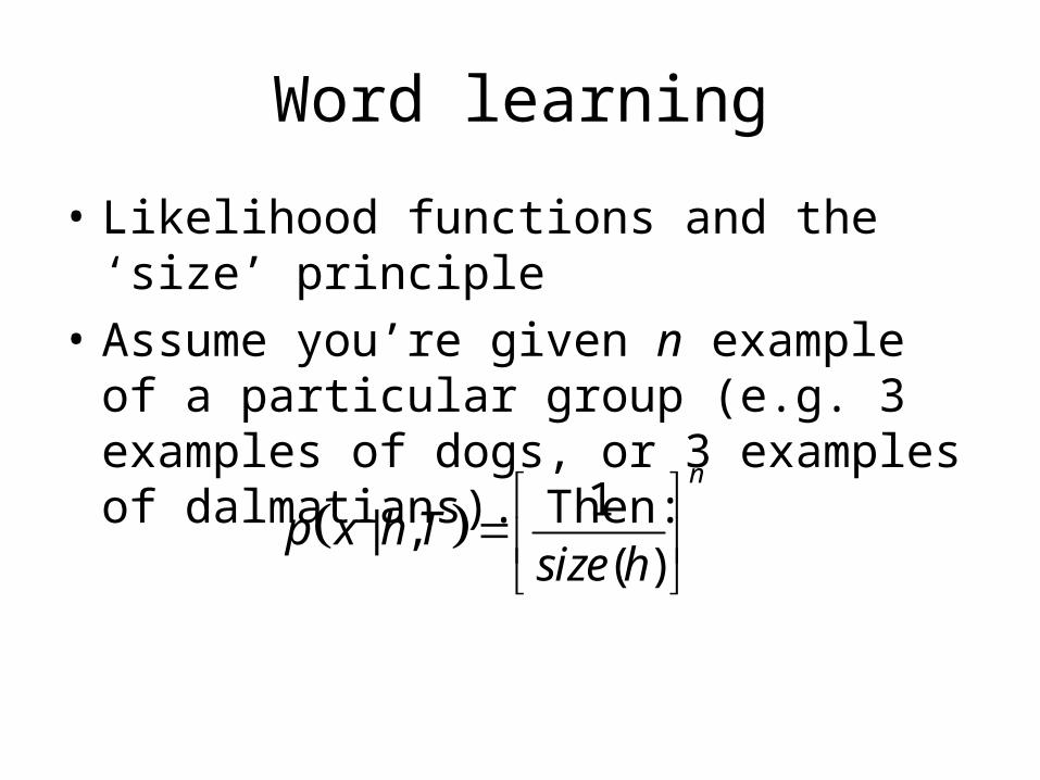
Word learning
• Likelihood functions and the ‘size’ principle
• Assume you’re given n example of a particular group (e.g. 3 examples of dogs, or 3 examples of dalmatians). Then:
1| ,
( )
n
p x h Tsize h
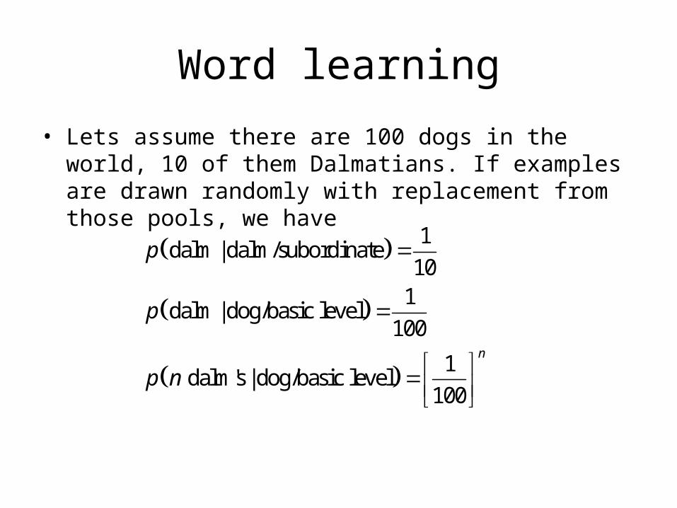
Word learning
• Lets assume there are 100 dogs in the world, 10 of them Dalmatians. If examples are drawn randomly with replacement from those pools, we have
1dalm | dalm/subordinate
101
dalm | dog/basic level100
1 dalm's | dog/basic level
100
n
p
p
p n
Word learning
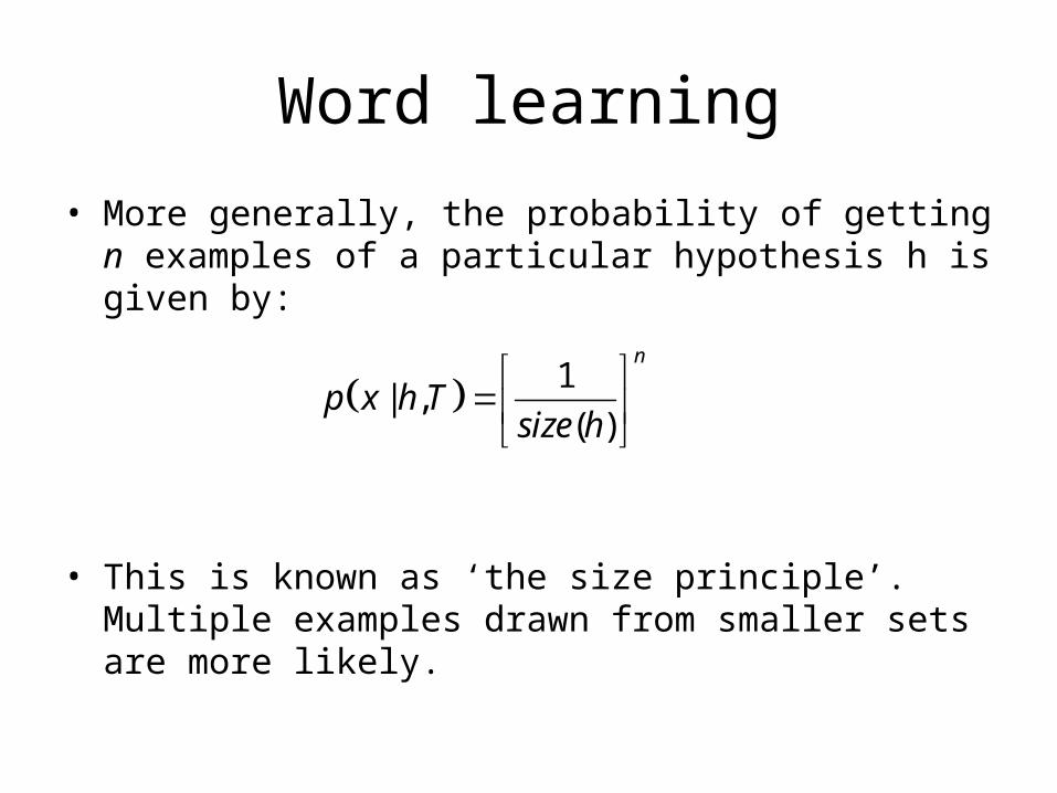
• More generally, the probability of getting n examples of a particular hypothesis h is given by:
• This is known as ‘the size principle’. Multiple examples drawn from smaller sets are more likely.
1| ,
( )
n
p x h Tsize h
Word learning
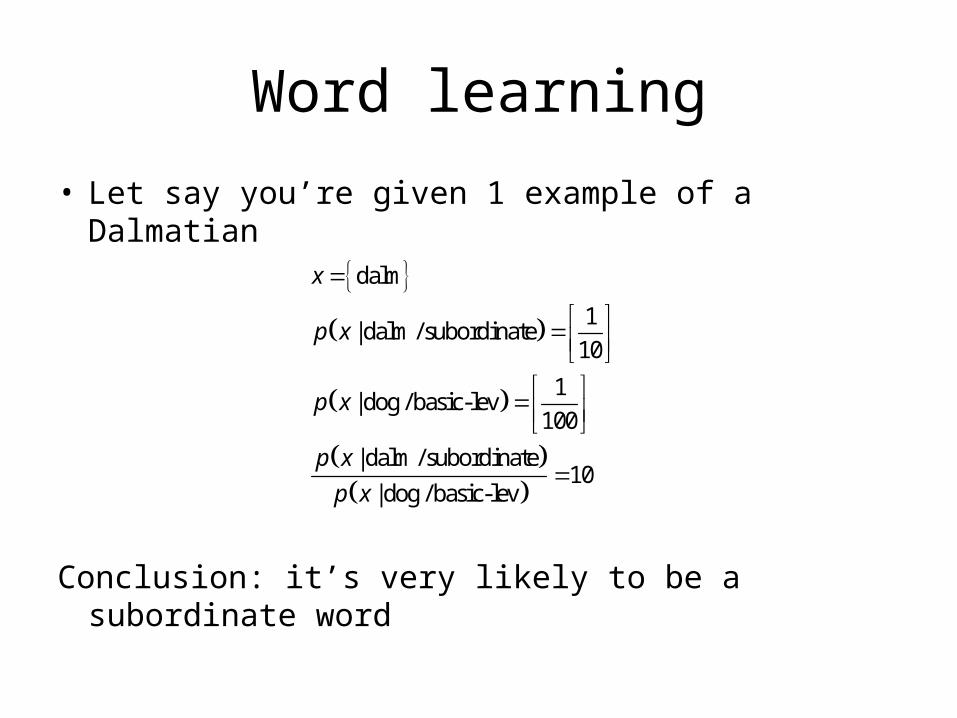
• Let say you’re given 1 example of a Dalmatian
Conclusion: it’s very likely to be a subordinate word
dalm
1| dalm / subordinate
10
1| dog / basic-lev
100
| dalm / subordinate10
| dog / basic-lev
x
p x
p x
p x
p x
Word learning
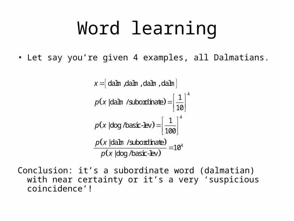
• Let say you’re given 4 examples, all Dalmatians.
Conclusion: it’s a subordinate word (dalmatian) with near certainty or it’s a very ‘suspicious coincidence’!
4
4
4
dalm,dalm, dalm, dalm
1| dalm / subordinate
10
1| dog / basic-lev
100
| dalm / subordinate10
| dog / basic-lev
x
p x
p x
p x
p x
Word learning
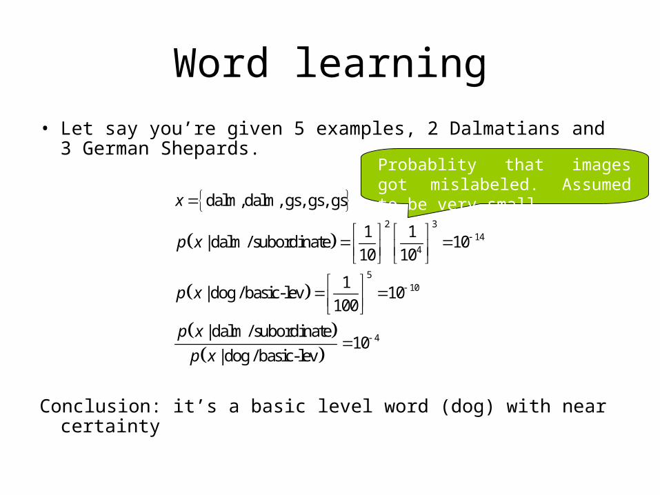
• Let say you’re given 5 examples, 2 Dalmatians and 3 German Shepards.
Conclusion: it’s a basic level word (dog) with near certainty
2 3
144
dalm,dalm, gs, gs, gs
1 1| dalm / subordinate 10
10 10
x
p x
Probablity that images got mislabeled. Assumed to be very small.
510
4
1| dog / basic-lev 10
100
| dalm / subordinate10
| dog / basic-lev
p x
p x
p x
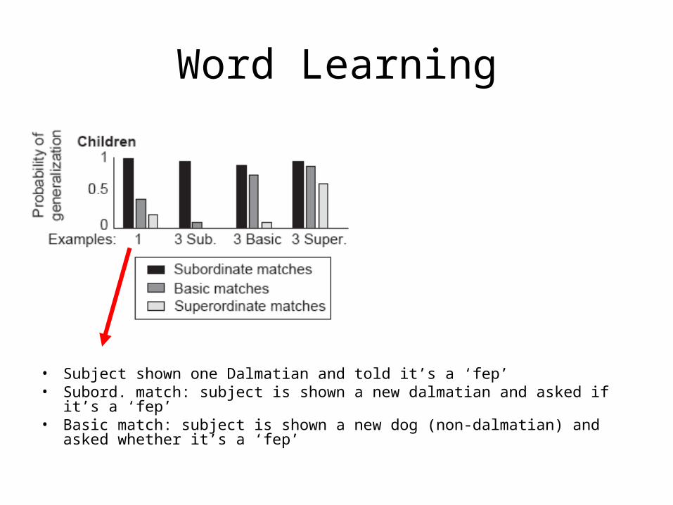
Word Learning
• Subject shown one Dalmatian and told it’s a ‘fep’• Subord. match: subject is shown a new dalmatian and asked if it’s a ‘fep’• Basic match: subject is shown a new dog (non-dalmatian) and asked whether it’s a
‘fep’
Word Learning
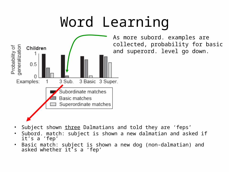
• Subject shown three Dalmatians and told they are ‘feps’• Subord. match: subject is shown a new dalmatian and asked if it’s a ‘fep’• Basic match: subject is shown a new dog (non-dalmatian) and asked whether it’s a
‘fep’
As more subord. examples are collected, probability for basic and superord. level go down.
Word Learning
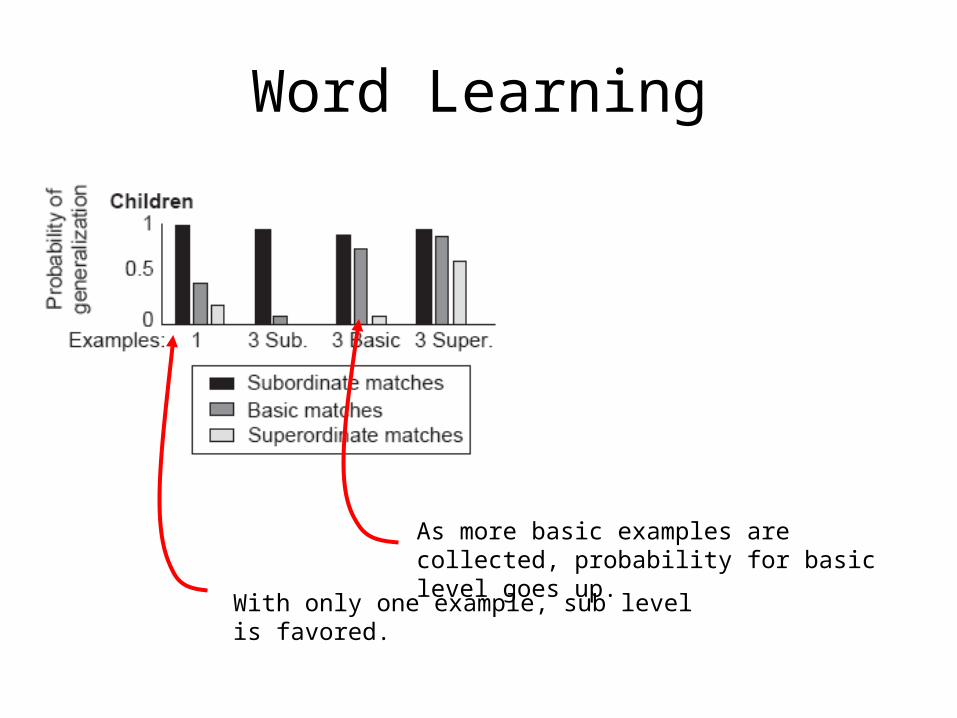
As more basic examples are collected, probability for basic level goes up.
With only one example, sub level is favored.
Word Learning
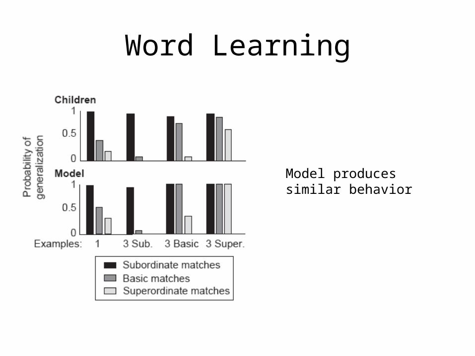
Model produces similar behavior


Bayesian property induction
Bayesian property induction
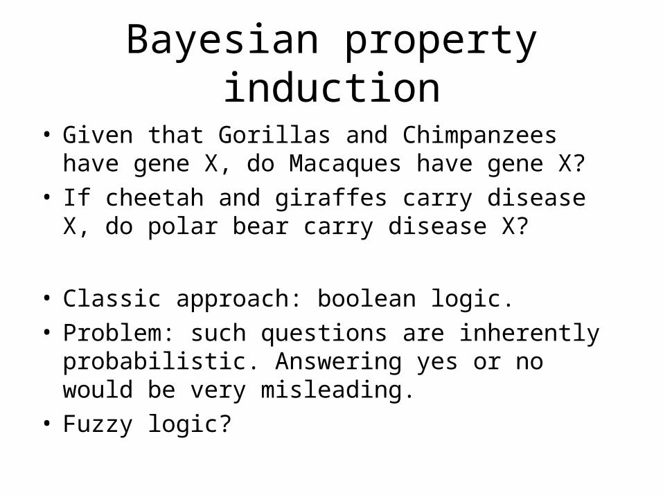
• Given that Gorillas and Chimpanzees have gene X, do Macaques have gene X?
• If cheetah and giraffes carry disease X, do polar bear carry disease X?
• Classic approach: boolean logic.• Problem: such questions are inherently probabilistic.
Answering yes or no would be very misleading. • Fuzzy logic?
Bayesian property induction
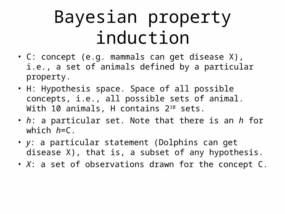
• C: concept (e.g. mammals can get disease X), i.e., a set of animals defined by a particular property.
• H: Hypothesis space. Space of all possible concepts, i.e., all possible sets of animal. With 10 animals, H contains 210 sets.
• h: a particular set. Note that there is an h for which h=C.
• y: a particular statement (Dolphins can get disease X), that is, a subset of any hypothesis.
• X: a set of observations drawn for the concept C.
Bayesian property induction
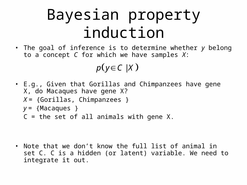
• The goal of inference is to determine whether y belong to a concept C for which we have samples X:
• E.g., Given that Gorillas and Chimpanzees have gene X, do Macaques have gene X?X = {Gorillas, Chimpanzees }y = {Macaques }C = the set of all animals with gene X.
• Note that we don’t know the full list of animal in set C. C is a hidden (or latent) variable. We need to integrate it out.
|p y C X
Bayesian property induction
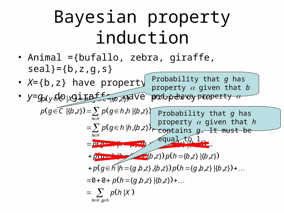
• Animal ={bufallo, zebra, giraffe, seal}={b,z,g,s}
• X={b,z} have property • y=g, do giraffes have property
,
|{ , } , |{ , }
| ,{ , } |{ , }
| { },{ , } { }|{ , } ...
| { , },{ , } { , }|{ , }
| { , , },{ , } { , , }|{ , }
0 0 { , , }|{ , }
|
h H
h H
h H g h
p g C b z p g h h b z
p g h h b z p h b z
p g h h s b z p h s b z
p g h h b z b z p h b z b z
p g h h g b z b z p h g b z b z
p h g b z b z
p h X
Probability that g has property given that h contains g. It must be equal to 1.
| |{ , }p y C X p g C b z
Probability that g has property given that b and z have property
Bayesian property induction
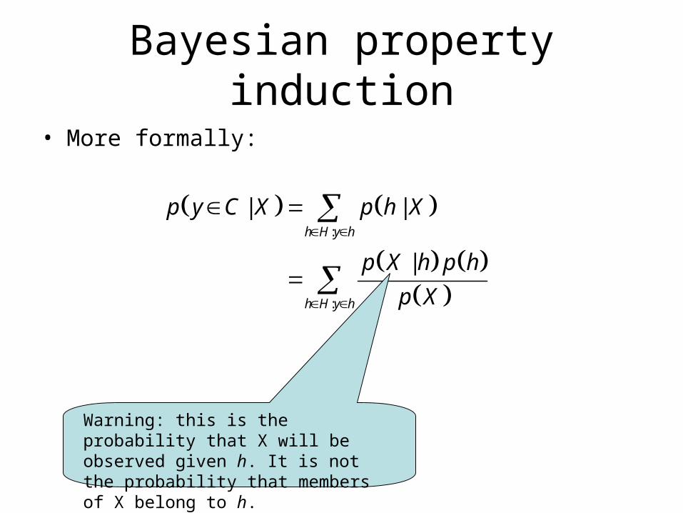
• More formally:
:
:
| |
|
h H y h
h H y h
p y C X p h X
p X h p h
p X
Warning: this is the probability that X will be observed given h. It is not the probability that members of X belong to h.
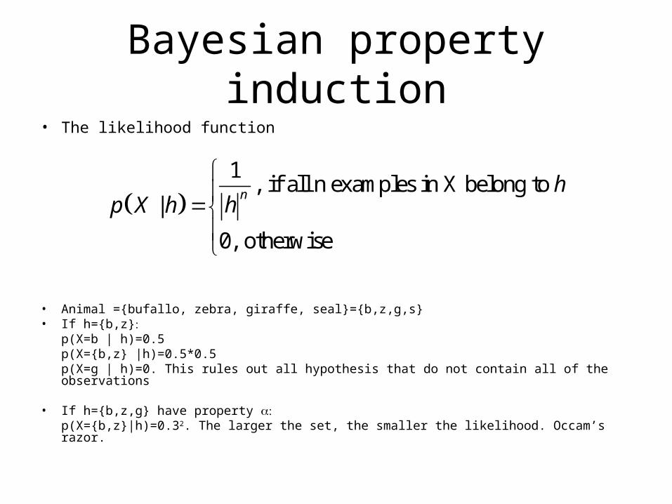
Bayesian property induction• The likelihood function
• Animal ={bufallo, zebra, giraffe, seal}={b,z,g,s}• If h={b,z}
p(X=b | h)=0.5p(X={b,z} |h)=0.5*0.5p(X=g | h)=0. This rules out all hypothesis that do not contain all of the observations
• If h={b,z,g} have property p(X={b,z}|h)=0.32. The larger the set, the smaller the likelihood. Occam’s razor.
1
, if all n examples in X belong to |
0, otherwise
n hhp X h
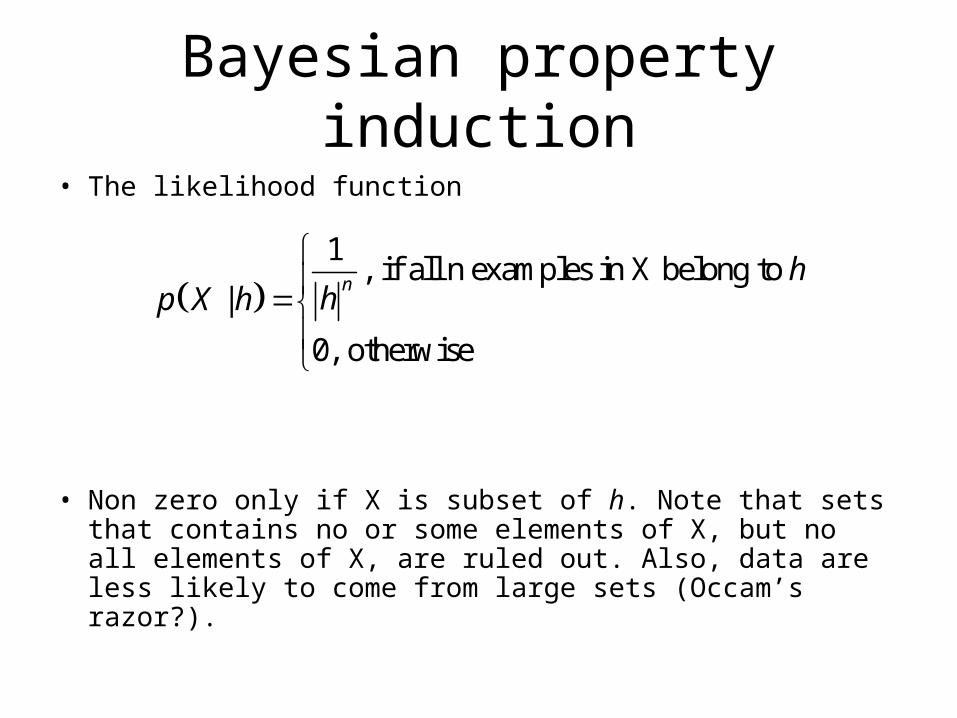
Bayesian property induction
• The likelihood function
• Non zero only if X is subset of h. Note that sets that contains no or some elements of X, but no all elements of X, are ruled out. Also, data are less likely to come from large sets (Occam’s razor?).
1
, if all n examples in X belong to |
0, otherwise
n hhp X h
Bayesian property induction
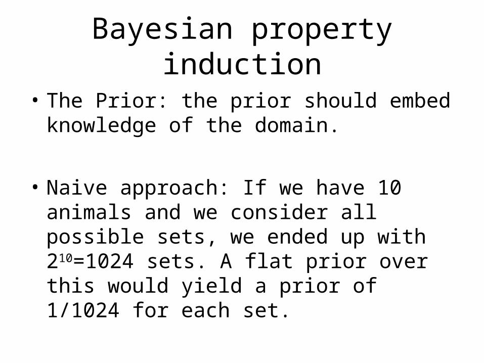
• The Prior: the prior should embed knowledge of the domain.
• Naive approach: If we have 10 animals and we consider all possible sets, we ended up with 210=1024 sets. A flat prior over this would yield a prior of 1/1024 for each set.
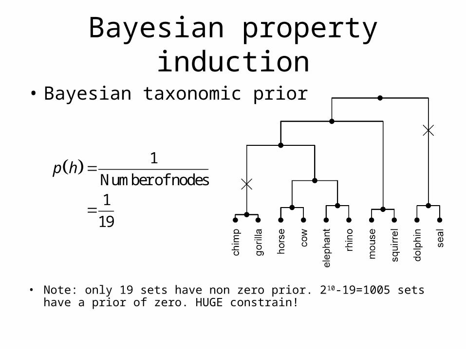
• Bayesian taxonomic prior
• Note: only 19 sets have non zero prior. 210-19=1005 sets have a prior of zero. HUGE constrain!
Bayesian property induction
1
Number of nodes1
19
p h
Bayesian property induction
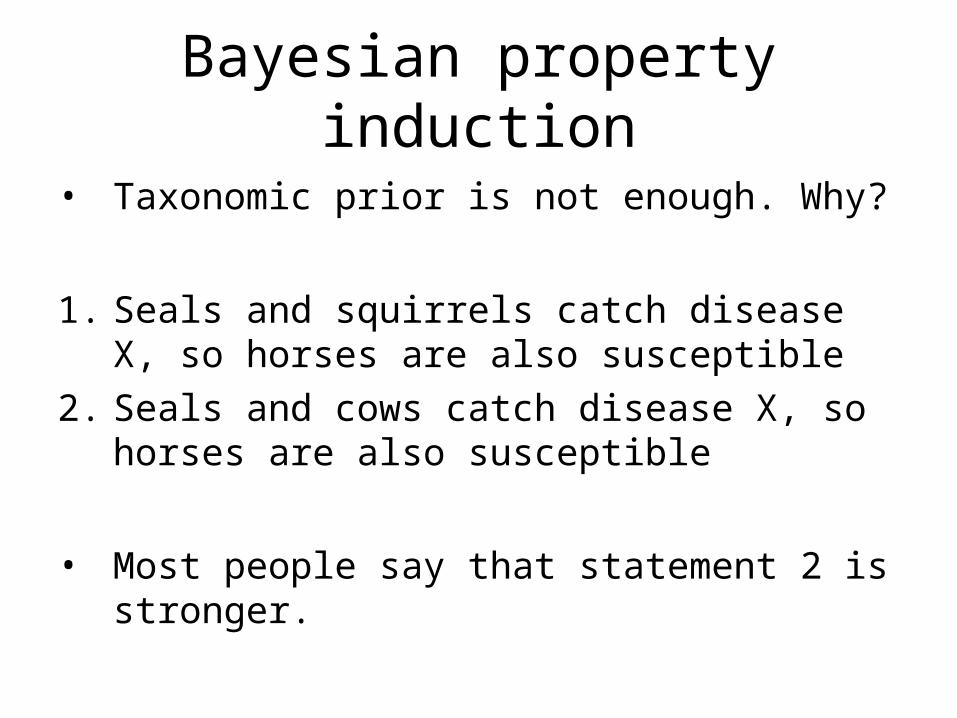
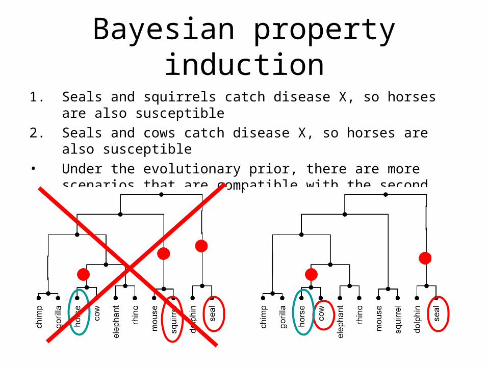
• Taxonomic prior is not enough. Why?
1. Seals and squirrels catch disease X, so horses are also susceptible
2. Seals and cows catch disease X, so horses are also susceptible
• Most people say that statement 2 is stronger.
Bayesian property induction
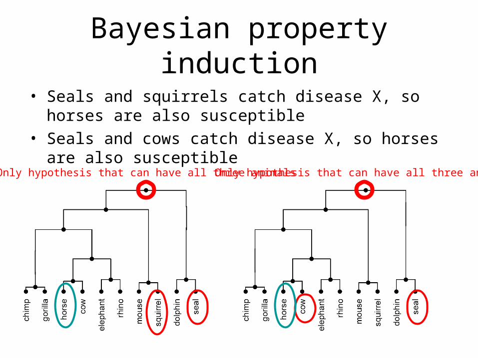
• Seals and squirrels catch disease X, so horses are also susceptible
• Seals and cows catch disease X, so horses are also susceptible
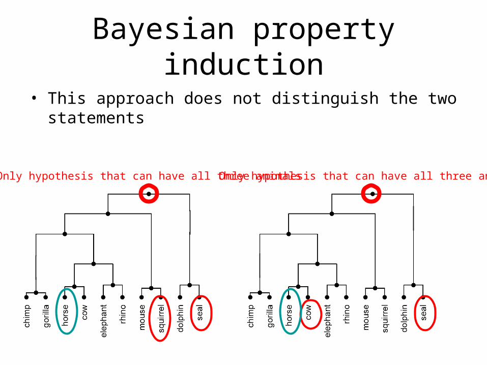
Only hypothesis that can have all three animals Only hypothesis that can have all three animals
Bayesian property induction
• This approach does not distinguish the two statements
Only hypothesis that can have all three animals Only hypothesis that can have all three animals
Bayesian property induction
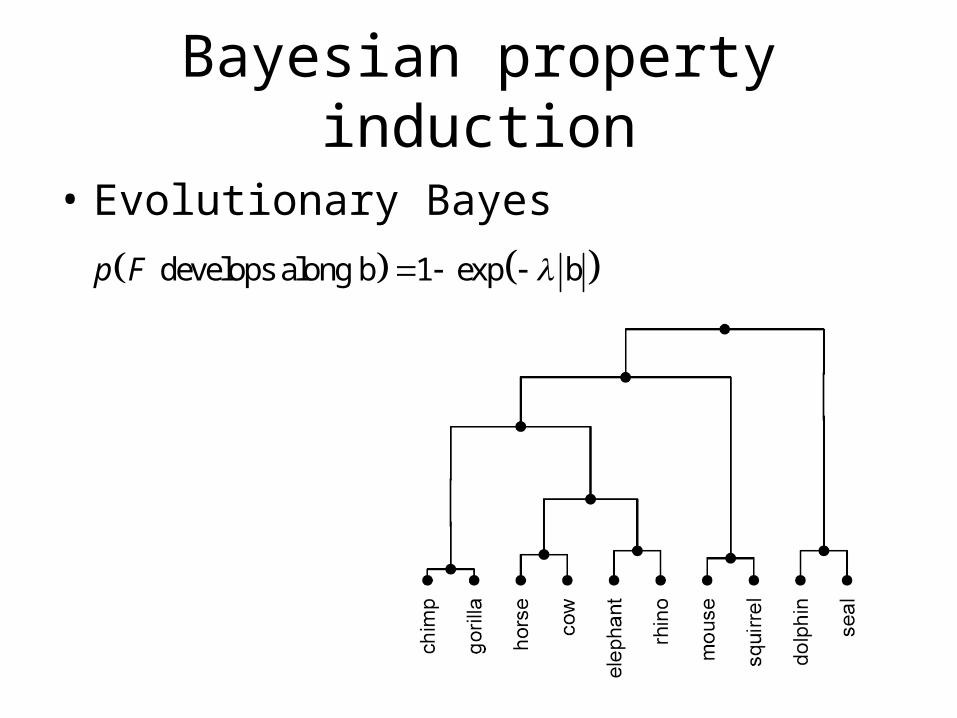
• Evolutionary Bayes
develops along b 1 exp bp F
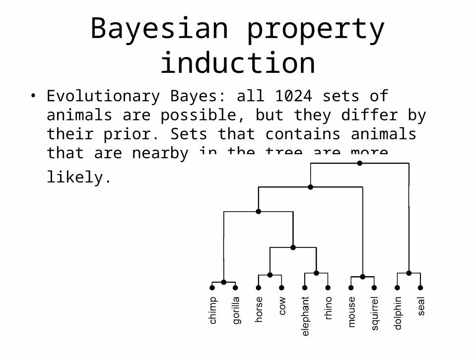
Bayesian property induction
• Evolutionary Bayes: all 1024 sets of animals are possible, but they differ by their prior. Sets that contains animals that are
nearby in the tree are more likely.
Bayesian property induction
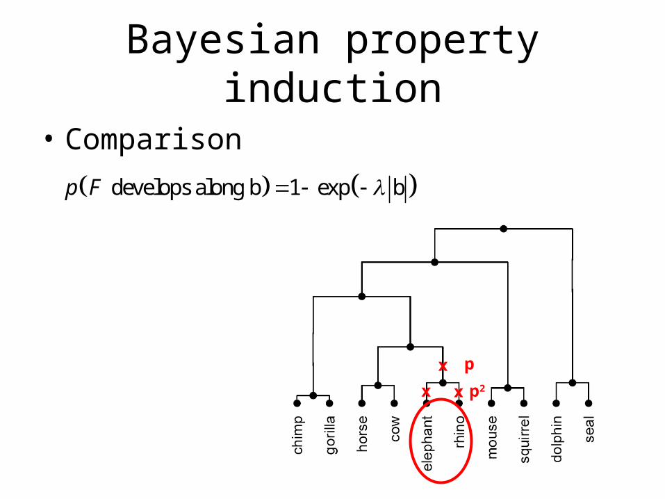
• Comparison
develops along b 1 exp bp F
x
x x
p
p2
Bayesian property induction
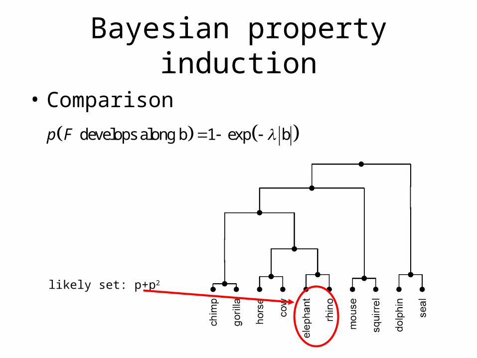
• Comparison
develops along b 1 exp bp F
likely set: p+p2

Bayesian property induction
• Comparison
develops along b 1 exp bp F
unlikely set: p2 x x
Bayesian property induction
1. Seals and squirrels catch disease X, so horses are also susceptible
2. Seals and cows catch disease X, so horses are also susceptible
• Under the evolutionary prior, there are more scenarios that are compatible with the second statement.

Bayesian property induction
• Evolutionary prior explain the data better than any other model (but not by much…).
Other priors
How to learn the structure of the prior
• Syntactic rules for growing graphs


Theory-based causal inference
Theory-based causal inference
• Can we use this framework to infer causality?
Theory-based causal inference
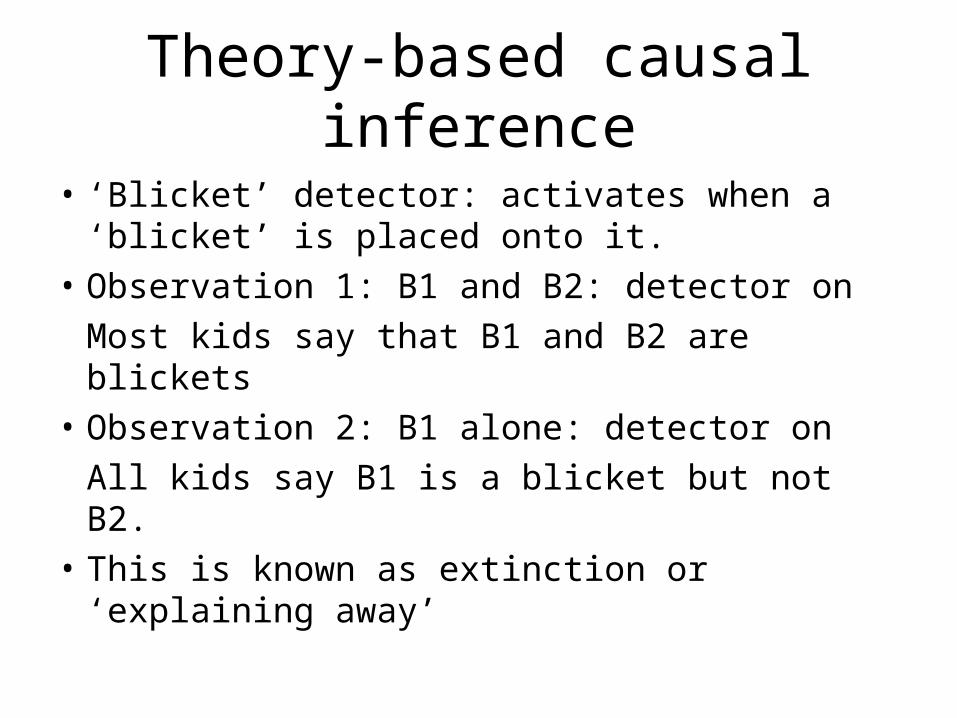
• ‘Blicket’ detector: activates when a ‘blicket’ is placed onto it.
• Observation 1: B1 and B2: detector on
Most kids say that B1 and B2 are blickets
• Observation 2: B1 alone: detector on
All kids say B1 is a blicket but not B2.
• This is known as extinction or ‘explaining away’
Theory-based causal inference
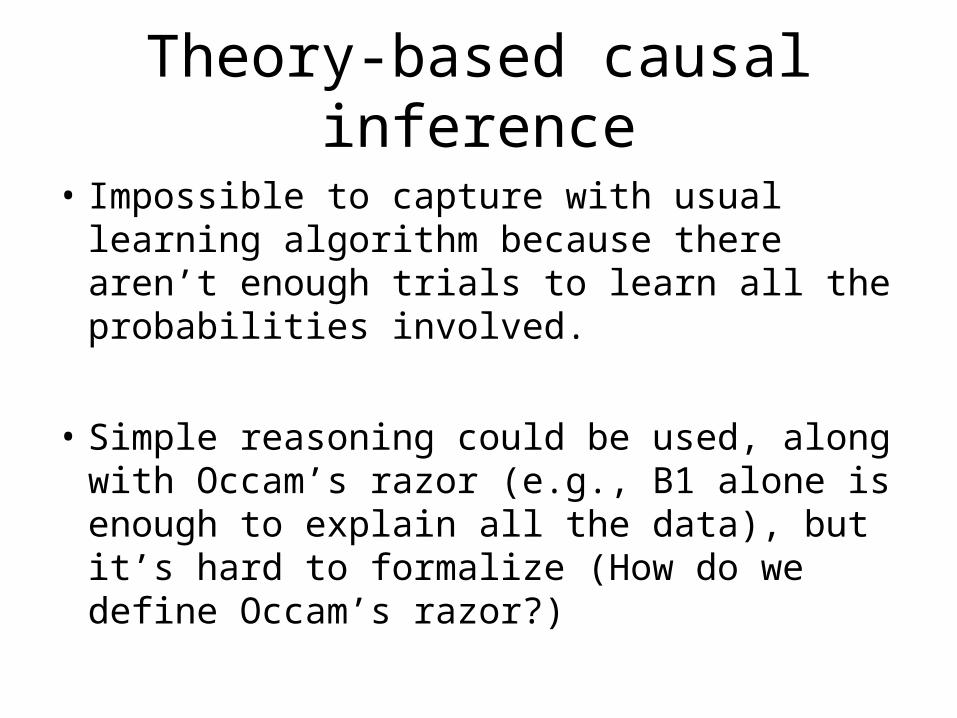
• Impossible to capture with usual learning algorithm because there aren’t enough trials to learn all the probabilities involved.
• Simple reasoning could be used, along with Occam’s razor (e.g., B1 alone is enough to explain all the data), but it’s hard to formalize (How do we define Occam’s razor?)
Theory-based causal inference
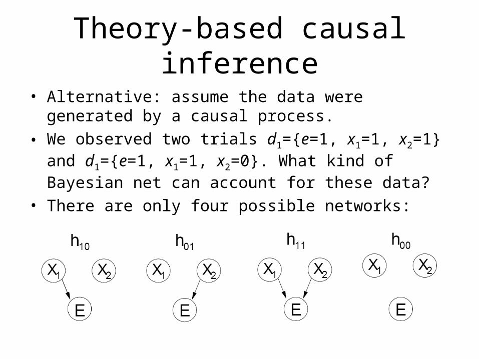
• Alternative: assume the data were generated by a causal process.
• We observed two trials d1={e=1, x1=1, x2=1} and d1={e=1, x1=1, x2=0}. What kind of Bayesian net can account for these data?
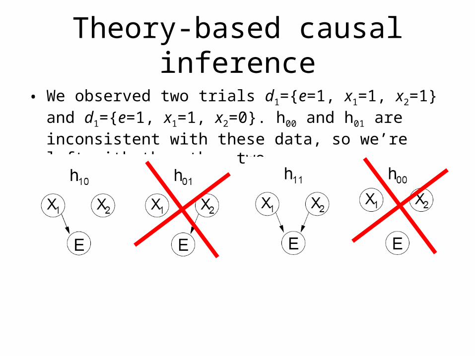
• There are only four possible networks:
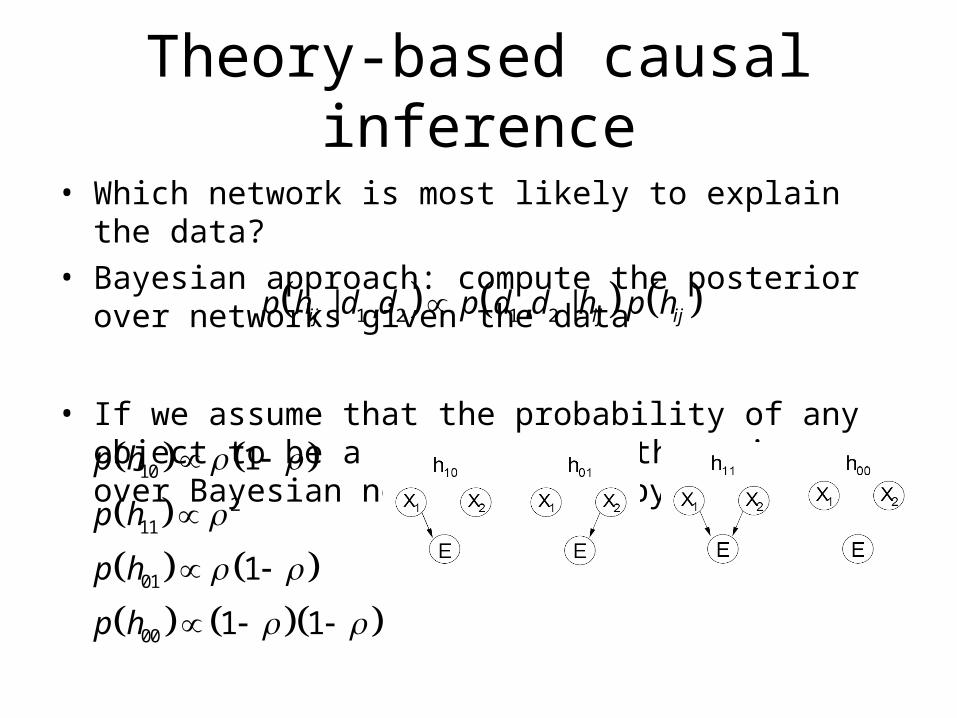
Theory-based causal inference
• Which network is most likely to explain the data?
• Bayesian approach: compute the posterior over networks given the data
• If we assume that the probability of any object to be a blicket is the prior over Bayesian nets is given by
1 2 1 2| , , |ij ij ijp h d d p d d h p h
10
211
01
00
1
1
1 1
p h
p h
p h
p h
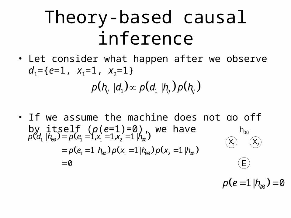
Theory-based causal inference
• Let consider what happen after we observe d1={e=1, x1=1, x2=1}
• If we assume the machine does not go off by itself (p(e=1)=0), we have
1 1| |ij ij ijp h d p d h p h
001| 0p e h
1 00 1 1 2 00
1 00 1 00 2 00
| 1, 1, 1|
1| 1| 1|
0
p d h p e x x h
p e h p x h p x h
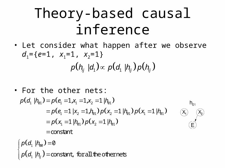
Theory-based causal inference
• Let consider what happen after we observe d1={e=1, x1=1, x2=1}
• For the other nets:
1 1| |ij ij ijp h d p d h p h
1 00
1
| 0
| constant, for all the other netsij
p d h
p d h
1 01 1 1 2 01
1 2 01 2 01 1 01
1 01 2 01
| 1, 1, 1|
1| 1, 1| 1|
1| 1|
constant
p d h p e x x h
p e x h p x h p x h
p x h p x h
Theory-based causal inference
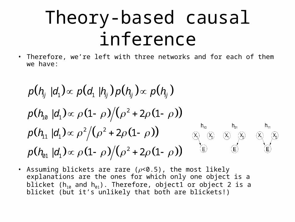
• Therefore, we’re left with three networks and for each of them we have:
• Assuming blickets are rare (<0.5), the most likely explanations are the ones for which only one object is a blicket (h10 and h01). Therefore, object1 or object 2 is a blicket (but it’s unlikely that both are blickets!)
1 1| |ij ij ij ijp h d p d h p h p h
210 1
2 211 1
201 1
| 1 2 1
| 2 1
| 1 2 1
p h d
p h d
p h d

Theory-based causal inference
• We now observe d2={e=1, x1=1, x2=0}
• Again, if we assume the machine does not go off by itself (p(e=1)=0), we have
1 2 1 2| , , |ij ij ijp h d d p d d h p h
1 2 01
1 2
, | 0
, | 1 otherwiseij
p d d h
p d d h
2 01 1 1 2 01
1 2 01 1 01 2 01
| 1, 1, 0 |
1| 0, 1| 0 |
0
p d h p e x x h
p e x h p x h p x h
We’re assuming that the machine does not go off if there is no ‘blicket’
1 2 001| 0, 0p e x h
Theory-based causal inference
• We observed two trials d1={e=1, x1=1, x2=1} and d1={e=1, x1=1, x2=0}. h00 and h01 are inconsistent with these data, so we’re left with the other two.
Theory-based causal inference
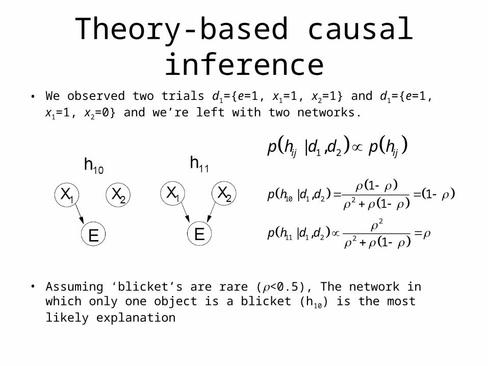
• We observed two trials d1={e=1, x1=1, x2=1} and d1={e=1, x1=1, x2=0} and we’re left with two networks.
• Assuming ‘blicket’s are rare (<0.5), The network in which only one object is a blicket (h10) is the most likely explanation
10 1 2 2
2
11 1 2 2
1| , 1
1
| ,1
p h d d
p h d d
1 2| ,ij ijp h d d p h
Theory-based causal inference
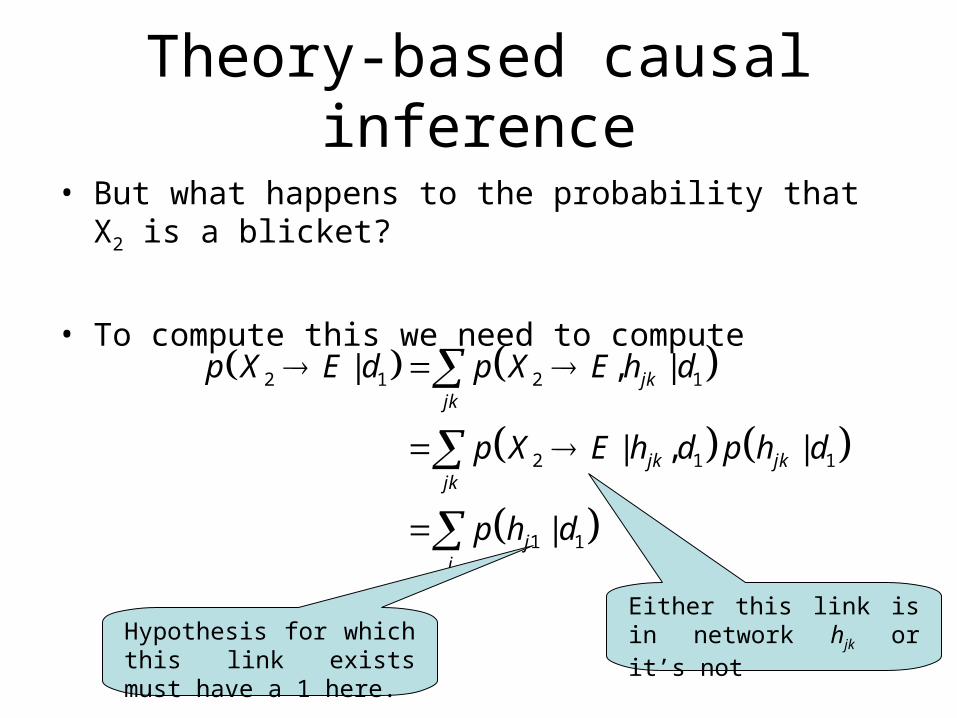
• But what happens to the probability that X2 is a blicket?
• To compute this we need to compute
2 1 2 1
2 1 1
1 1
| , |
| , |
|
jkjk
jk jkjk
jj
p X E d p X E h d
p X E h d p h d
p h d
Either this link is in network hjk or it’s notHypothesis for which this link
exists must have a 1 here.
Theory-based causal inference
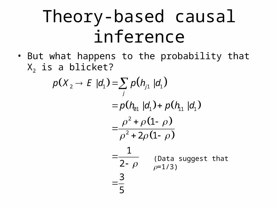
• But what happens to the probability that X2 is a blicket?
2 1 1 1
01 1 11 1
2
2
| |
| |
1
2 1
1
2
3
5
jj
p X E d p h d
p h d p h d
(Data suggest that =1/3)
Theory-based causal inference
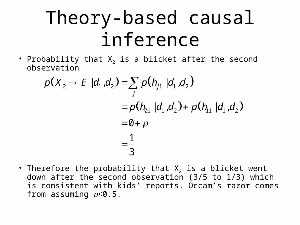
• Probability that X2 is a blicket after the second observation
• Therefore the probability that X2 is a blicket went down after the second observation (3/5 to 1/3) which is consistent with kids’ reports. Occam’s razor comes from assuming <0.5.
2 1 2 1 1 2
01 1 2 11 1 2
| , | ,
| , | ,
0
1
3
jj
p X E d d p h d d
p h d d p h d d
Theory-based causal inference
• This approach can be generalized to much more complicated generative models.