bayesian biostatistics - usp · bayesian biostatistics emmanuel lesaffre interuniversity institute...
TRANSCRIPT
Bayesian Biostatistics
Emmanuel LesaffreInteruniversity Institute for Biostatistics and statistical Bioinformatics
KU Leuven & University Hasselt
Departamento de Ciencias Exatas — University of Piracicaba
8 to 12 December 2014

Contents
I Basic concepts in Bayesian methods 1
0.1 Preface . . . . . . . . . . . . . . . . . . . . . . . . . . . . . . . . . . . . . . . . . . . . . . . . . . . . . . . . . . . . . . . . 2
0.2 Time schedule of the course . . . . . . . . . . . . . . . . . . . . . . . . . . . . . . . . . . . . . . . . . . . . . . . . . . . . . 7
0.3 Aims of the course . . . . . . . . . . . . . . . . . . . . . . . . . . . . . . . . . . . . . . . . . . . . . . . . . . . . . . . . . . 9
1 Modes of statistical inference . . . . . . . . . . . . . . . . . . . . . . . . . . . . . . . . . . . . . . . . . . . . . . . . . . . . . . . . . . . . . . . . . . . . . . . . . . . . . . . . . . . 10
1.1 The frequentist approach: a critical reflection . . . . . . . . . . . . . . . . . . . . . . . . . . . . . . . . . . . . . . . . . . . . 11
1.1.1 The classical statistical approach . . . . . . . . . . . . . . . . . . . . . . . . . . . . . . . . . . . . . . . . . . . . . . 12
1.1.2 The P -value as a measure of evidence . . . . . . . . . . . . . . . . . . . . . . . . . . . . . . . . . . . . . . . . . . . 15
1.1.3 The confidence interval as a measure of evidence . . . . . . . . . . . . . . . . . . . . . . . . . . . . . . . . . . . . . . 26
1.2 Statistical inference based on the likelihood function . . . . . . . . . . . . . . . . . . . . . . . . . . . . . . . . . . . . . . . . 28
Bayesian Biostatistics - Piracicaba 2014 i

1.2.1 The likelihood function . . . . . . . . . . . . . . . . . . . . . . . . . . . . . . . . . . . . . . . . . . . . . . . . . . . 29
1.2.2 The likelihood principles . . . . . . . . . . . . . . . . . . . . . . . . . . . . . . . . . . . . . . . . . . . . . . . . . . . 34
1.3 The Bayesian approach: some basic ideas . . . . . . . . . . . . . . . . . . . . . . . . . . . . . . . . . . . . . . . . . . . . . . 43
1.3.1 Introduction . . . . . . . . . . . . . . . . . . . . . . . . . . . . . . . . . . . . . . . . . . . . . . . . . . . . . . . . . 44
1.3.2 Bayes theorem – Discrete version for simple events - 1 . . . . . . . . . . . . . . . . . . . . . . . . . . . . . . . . . . . 48
1.4 Outlook . . . . . . . . . . . . . . . . . . . . . . . . . . . . . . . . . . . . . . . . . . . . . . . . . . . . . . . . . . . . . . . 54
2 Bayes theorem: computing the posterior distribution . . . . . . . . . . . . . . . . . . . . . . . . . . . . . . . . . . . . . . . . . . . . . . . . . . . . . . . . . . . . . 59
2.1 Introduction . . . . . . . . . . . . . . . . . . . . . . . . . . . . . . . . . . . . . . . . . . . . . . . . . . . . . . . . . . . . . 60
2.2 Bayes theorem – The binary version . . . . . . . . . . . . . . . . . . . . . . . . . . . . . . . . . . . . . . . . . . . . . . . . . 61
2.3 Probability in a Bayesian context . . . . . . . . . . . . . . . . . . . . . . . . . . . . . . . . . . . . . . . . . . . . . . . . . . 63
2.4 Bayes theorem – The categorical version . . . . . . . . . . . . . . . . . . . . . . . . . . . . . . . . . . . . . . . . . . . . . . 66
2.5 Bayes theorem – The continuous version . . . . . . . . . . . . . . . . . . . . . . . . . . . . . . . . . . . . . . . . . . . . . . 67
2.6 The binomial case . . . . . . . . . . . . . . . . . . . . . . . . . . . . . . . . . . . . . . . . . . . . . . . . . . . . . . . . . . 69
2.7 The Gaussian case . . . . . . . . . . . . . . . . . . . . . . . . . . . . . . . . . . . . . . . . . . . . . . . . . . . . . . . . . . 87
2.8 The Poisson case . . . . . . . . . . . . . . . . . . . . . . . . . . . . . . . . . . . . . . . . . . . . . . . . . . . . . . . . . . . 102
Bayesian Biostatistics - Piracicaba 2014 ii
2.9 The prior and posterior of derived parameter . . . . . . . . . . . . . . . . . . . . . . . . . . . . . . . . . . . . . . . . . . . . 113
2.10 Bayesian versus likelihood approach . . . . . . . . . . . . . . . . . . . . . . . . . . . . . . . . . . . . . . . . . . . . . . . . . 116
2.11 Bayesian versus frequentist approach . . . . . . . . . . . . . . . . . . . . . . . . . . . . . . . . . . . . . . . . . . . . . . . . 117
2.12 The different modes of the Bayesian approach . . . . . . . . . . . . . . . . . . . . . . . . . . . . . . . . . . . . . . . . . . . 119
2.13 An historical note on the Bayesian approach . . . . . . . . . . . . . . . . . . . . . . . . . . . . . . . . . . . . . . . . . . . . 120
3 Introduction to Bayesian inference . . . . . . . . . . . . . . . . . . . . . . . . . . . . . . . . . . . . . . . . . . . . . . . . . . . . . . . . . . . . . . . . . . . . . . . . . . . . . . 127
3.1 Introduction . . . . . . . . . . . . . . . . . . . . . . . . . . . . . . . . . . . . . . . . . . . . . . . . . . . . . . . . . . . . . 128
3.2 Summarizing the posterior with probabilities . . . . . . . . . . . . . . . . . . . . . . . . . . . . . . . . . . . . . . . . . . . . 129
3.3 Posterior summary measures . . . . . . . . . . . . . . . . . . . . . . . . . . . . . . . . . . . . . . . . . . . . . . . . . . . . . 130
3.3.1 Posterior mode, mean, median, variance and SD . . . . . . . . . . . . . . . . . . . . . . . . . . . . . . . . . . . . . . 131
3.3.2 Credible/credibility interval . . . . . . . . . . . . . . . . . . . . . . . . . . . . . . . . . . . . . . . . . . . . . . . . . 135
3.4 Predictive distributions . . . . . . . . . . . . . . . . . . . . . . . . . . . . . . . . . . . . . . . . . . . . . . . . . . . . . . . . 140
3.4.1 Introduction . . . . . . . . . . . . . . . . . . . . . . . . . . . . . . . . . . . . . . . . . . . . . . . . . . . . . . . . . 141
3.4.2 Posterior predictive distribution: General case . . . . . . . . . . . . . . . . . . . . . . . . . . . . . . . . . . . . . . . . 148
3.5 Exchangeability . . . . . . . . . . . . . . . . . . . . . . . . . . . . . . . . . . . . . . . . . . . . . . . . . . . . . . . . . . . . 157
Bayesian Biostatistics - Piracicaba 2014 iii
3.6 A normal approximation to the posterior . . . . . . . . . . . . . . . . . . . . . . . . . . . . . . . . . . . . . . . . . . . . . . 158
3.7 Numerical techniques to determine the posterior . . . . . . . . . . . . . . . . . . . . . . . . . . . . . . . . . . . . . . . . . . 159
3.7.1 Numerical integration . . . . . . . . . . . . . . . . . . . . . . . . . . . . . . . . . . . . . . . . . . . . . . . . . . . . 160
3.7.2 Sampling from the posterior distribution . . . . . . . . . . . . . . . . . . . . . . . . . . . . . . . . . . . . . . . . . . 162
3.7.3 Choice of posterior summary measures . . . . . . . . . . . . . . . . . . . . . . . . . . . . . . . . . . . . . . . . . . . 175
3.8 Bayesian hypothesis testing . . . . . . . . . . . . . . . . . . . . . . . . . . . . . . . . . . . . . . . . . . . . . . . . . . . . . 176
3.8.1 The Bayes factor . . . . . . . . . . . . . . . . . . . . . . . . . . . . . . . . . . . . . . . . . . . . . . . . . . . . . . . 183
3.9 Medical literature on Bayesian methods in RCTs . . . . . . . . . . . . . . . . . . . . . . . . . . . . . . . . . . . . . . . . . . 185
4 More than one parameter . . . . . . . . . . . . . . . . . . . . . . . . . . . . . . . . . . . . . . . . . . . . . . . . . . . . . . . . . . . . . . . . . . . . . . . . . . . . . . . . . . . . . . . 196
4.1 Introduction . . . . . . . . . . . . . . . . . . . . . . . . . . . . . . . . . . . . . . . . . . . . . . . . . . . . . . . . . . . . . 197
4.2 Joint versus marginal posterior inference . . . . . . . . . . . . . . . . . . . . . . . . . . . . . . . . . . . . . . . . . . . . . . 199
4.3 The normal distribution with µ and σ2 unknown . . . . . . . . . . . . . . . . . . . . . . . . . . . . . . . . . . . . . . . . . . 201
4.3.1 No prior knowledge on µ and σ2 is available . . . . . . . . . . . . . . . . . . . . . . . . . . . . . . . . . . . . . . . . 202
4.3.2 An historical study is available . . . . . . . . . . . . . . . . . . . . . . . . . . . . . . . . . . . . . . . . . . . . . . . . 214
4.3.3 Expert knowledge is available . . . . . . . . . . . . . . . . . . . . . . . . . . . . . . . . . . . . . . . . . . . . . . . . 218
Bayesian Biostatistics - Piracicaba 2014 iv

4.4 Multivariate distributions . . . . . . . . . . . . . . . . . . . . . . . . . . . . . . . . . . . . . . . . . . . . . . . . . . . . . . 220
4.5 Frequentist properties of Bayesian inference . . . . . . . . . . . . . . . . . . . . . . . . . . . . . . . . . . . . . . . . . . . . . 227
4.6 The Method of Composition . . . . . . . . . . . . . . . . . . . . . . . . . . . . . . . . . . . . . . . . . . . . . . . . . . . . . 228
4.7 Bayesian linear regression models . . . . . . . . . . . . . . . . . . . . . . . . . . . . . . . . . . . . . . . . . . . . . . . . . . 231
4.7.1 The frequentist approach to linear regression . . . . . . . . . . . . . . . . . . . . . . . . . . . . . . . . . . . . . . . . 232
4.7.2 A noninformative Bayesian linear regression model . . . . . . . . . . . . . . . . . . . . . . . . . . . . . . . . . . . . . 235
4.7.3 Posterior summary measures for the linear regression model . . . . . . . . . . . . . . . . . . . . . . . . . . . . . . . . 236
4.7.4 Sampling from the posterior distribution . . . . . . . . . . . . . . . . . . . . . . . . . . . . . . . . . . . . . . . . . . 239
4.8 Bayesian generalized linear models . . . . . . . . . . . . . . . . . . . . . . . . . . . . . . . . . . . . . . . . . . . . . . . . . . 243
4.8.1 More complex regression models . . . . . . . . . . . . . . . . . . . . . . . . . . . . . . . . . . . . . . . . . . . . . . . 244
5 Choosing the prior distribution . . . . . . . . . . . . . . . . . . . . . . . . . . . . . . . . . . . . . . . . . . . . . . . . . . . . . . . . . . . . . . . . . . . . . . . . . . . . . . . . . . 246
5.1 Introduction . . . . . . . . . . . . . . . . . . . . . . . . . . . . . . . . . . . . . . . . . . . . . . . . . . . . . . . . . . . . . 247
5.2 The sequential use of Bayes theorem . . . . . . . . . . . . . . . . . . . . . . . . . . . . . . . . . . . . . . . . . . . . . . . . 248
5.3 Conjugate prior distributions . . . . . . . . . . . . . . . . . . . . . . . . . . . . . . . . . . . . . . . . . . . . . . . . . . . . . 249
5.3.1 Conjugate priors for univariate data distributions . . . . . . . . . . . . . . . . . . . . . . . . . . . . . . . . . . . . . . 250
Bayesian Biostatistics - Piracicaba 2014 v

5.3.2 Conjugate prior for normal distribution – mean and variance unknown . . . . . . . . . . . . . . . . . . . . . . . . . . . 258
5.3.3 Multivariate data distributions . . . . . . . . . . . . . . . . . . . . . . . . . . . . . . . . . . . . . . . . . . . . . . . . 260
5.3.4 Conditional conjugate and semi-conjugate priors . . . . . . . . . . . . . . . . . . . . . . . . . . . . . . . . . . . . . . 264
5.3.5 Hyperpriors . . . . . . . . . . . . . . . . . . . . . . . . . . . . . . . . . . . . . . . . . . . . . . . . . . . . . . . . . . 265
5.4 Noninformative prior distributions . . . . . . . . . . . . . . . . . . . . . . . . . . . . . . . . . . . . . . . . . . . . . . . . . . 266
5.4.1 Introduction . . . . . . . . . . . . . . . . . . . . . . . . . . . . . . . . . . . . . . . . . . . . . . . . . . . . . . . . . 267
5.4.2 Expressing ignorance . . . . . . . . . . . . . . . . . . . . . . . . . . . . . . . . . . . . . . . . . . . . . . . . . . . . . 268
5.4.3 General principles to choose noninformative priors . . . . . . . . . . . . . . . . . . . . . . . . . . . . . . . . . . . . . 271
5.4.4 Improper prior distributions . . . . . . . . . . . . . . . . . . . . . . . . . . . . . . . . . . . . . . . . . . . . . . . . . 273
5.4.5 Weak/vague priors . . . . . . . . . . . . . . . . . . . . . . . . . . . . . . . . . . . . . . . . . . . . . . . . . . . . . . 274
5.5 Informative prior distributions . . . . . . . . . . . . . . . . . . . . . . . . . . . . . . . . . . . . . . . . . . . . . . . . . . . . 279
5.5.1 Introduction . . . . . . . . . . . . . . . . . . . . . . . . . . . . . . . . . . . . . . . . . . . . . . . . . . . . . . . . . 280
5.5.2 Data-based prior distributions . . . . . . . . . . . . . . . . . . . . . . . . . . . . . . . . . . . . . . . . . . . . . . . . 285
5.5.3 Elicitation of prior knowledge . . . . . . . . . . . . . . . . . . . . . . . . . . . . . . . . . . . . . . . . . . . . . . . . 286
5.5.4 Archetypal prior distributions . . . . . . . . . . . . . . . . . . . . . . . . . . . . . . . . . . . . . . . . . . . . . . . . 294
Bayesian Biostatistics - Piracicaba 2014 vi

5.6 Prior distributions for regression models . . . . . . . . . . . . . . . . . . . . . . . . . . . . . . . . . . . . . . . . . . . . . . . 302
5.6.1 Normal linear regression . . . . . . . . . . . . . . . . . . . . . . . . . . . . . . . . . . . . . . . . . . . . . . . . . . . 303
5.6.2 Generalized linear models . . . . . . . . . . . . . . . . . . . . . . . . . . . . . . . . . . . . . . . . . . . . . . . . . . 305
5.7 Modeling priors . . . . . . . . . . . . . . . . . . . . . . . . . . . . . . . . . . . . . . . . . . . . . . . . . . . . . . . . . . . . 306
5.8 Other regression models . . . . . . . . . . . . . . . . . . . . . . . . . . . . . . . . . . . . . . . . . . . . . . . . . . . . . . . 311
6 Markov chain Monte Carlo sampling . . . . . . . . . . . . . . . . . . . . . . . . . . . . . . . . . . . . . . . . . . . . . . . . . . . . . . . . . . . . . . . . . . . . . . . . . . . . . 314
6.1 Introduction . . . . . . . . . . . . . . . . . . . . . . . . . . . . . . . . . . . . . . . . . . . . . . . . . . . . . . . . . . . . . 315
6.2 The Gibbs sampler . . . . . . . . . . . . . . . . . . . . . . . . . . . . . . . . . . . . . . . . . . . . . . . . . . . . . . . . . . 327
6.2.1 The bivariate Gibbs sampler . . . . . . . . . . . . . . . . . . . . . . . . . . . . . . . . . . . . . . . . . . . . . . . . . 328
6.2.2 The general Gibbs sampler . . . . . . . . . . . . . . . . . . . . . . . . . . . . . . . . . . . . . . . . . . . . . . . . . . 340
6.2.3 Remarks∗ . . . . . . . . . . . . . . . . . . . . . . . . . . . . . . . . . . . . . . . . . . . . . . . . . . . . . . . . . . . 353
6.2.4 Review of Gibbs sampling approaches . . . . . . . . . . . . . . . . . . . . . . . . . . . . . . . . . . . . . . . . . . . . 354
6.3 The Metropolis(-Hastings) algorithm . . . . . . . . . . . . . . . . . . . . . . . . . . . . . . . . . . . . . . . . . . . . . . . . 356
6.3.1 The Metropolis algorithm . . . . . . . . . . . . . . . . . . . . . . . . . . . . . . . . . . . . . . . . . . . . . . . . . . 357
6.3.2 The Metropolis-Hastings algorithm . . . . . . . . . . . . . . . . . . . . . . . . . . . . . . . . . . . . . . . . . . . . . 367
Bayesian Biostatistics - Piracicaba 2014 vii

6.3.3 Remarks* . . . . . . . . . . . . . . . . . . . . . . . . . . . . . . . . . . . . . . . . . . . . . . . . . . . . . . . . . . 370
7 Assessing and improving convergence of the Markov chain . . . . . . . . . . . . . . . . . . . . . . . . . . . . . . . . . . . . . . . . . . . . . . . . . . . . . . . . 376
7.1 Introduction . . . . . . . . . . . . . . . . . . . . . . . . . . . . . . . . . . . . . . . . . . . . . . . . . . . . . . . . . . . . . 377
7.2 Assessing convergence of a Markov chain . . . . . . . . . . . . . . . . . . . . . . . . . . . . . . . . . . . . . . . . . . . . . . 378
7.2.1 Definition of convergence for a Markov chain . . . . . . . . . . . . . . . . . . . . . . . . . . . . . . . . . . . . . . . . 379
7.2.2 Checking convergence of the Markov chain . . . . . . . . . . . . . . . . . . . . . . . . . . . . . . . . . . . . . . . . . 381
7.2.3 Graphical approaches to assess convergence . . . . . . . . . . . . . . . . . . . . . . . . . . . . . . . . . . . . . . . . . 382
7.2.4 Graphical approaches to assess convergence . . . . . . . . . . . . . . . . . . . . . . . . . . . . . . . . . . . . . . . . . 383
7.2.5 Formal approaches to assess convergence . . . . . . . . . . . . . . . . . . . . . . . . . . . . . . . . . . . . . . . . . . 394
7.2.6 Computing the Monte Carlo standard error . . . . . . . . . . . . . . . . . . . . . . . . . . . . . . . . . . . . . . . . . 409
7.2.7 Practical experience with the formal diagnostic procedures . . . . . . . . . . . . . . . . . . . . . . . . . . . . . . . . . 412
7.3 Accelerating convergence . . . . . . . . . . . . . . . . . . . . . . . . . . . . . . . . . . . . . . . . . . . . . . . . . . . . . . 414
7.4 Practical guidelines for assessing and accelerating convergence . . . . . . . . . . . . . . . . . . . . . . . . . . . . . . . . . . . 418
7.5 Data augmentation . . . . . . . . . . . . . . . . . . . . . . . . . . . . . . . . . . . . . . . . . . . . . . . . . . . . . . . . . 419
8 Software . . . . . . . . . . . . . . . . . . . . . . . . . . . . . . . . . . . . . . . . . . . . . . . . . . . . . . . . . . . . . . . . . . . . . . . . . . . . . . . . . . . . . . . . . . . . . . . . . . . . . . . 436
Bayesian Biostatistics - Piracicaba 2014 viii

8.1 WinBUGS and related software . . . . . . . . . . . . . . . . . . . . . . . . . . . . . . . . . . . . . . . . . . . . . . . . . . . 439
8.1.1 A first analysis . . . . . . . . . . . . . . . . . . . . . . . . . . . . . . . . . . . . . . . . . . . . . . . . . . . . . . . . 440
8.1.2 Information on samplers . . . . . . . . . . . . . . . . . . . . . . . . . . . . . . . . . . . . . . . . . . . . . . . . . . . 450
8.1.3 Assessing and accelerating convergence . . . . . . . . . . . . . . . . . . . . . . . . . . . . . . . . . . . . . . . . . . . 452
8.1.4 Vector and matrix manipulations . . . . . . . . . . . . . . . . . . . . . . . . . . . . . . . . . . . . . . . . . . . . . . 457
8.1.5 Working in batch mode . . . . . . . . . . . . . . . . . . . . . . . . . . . . . . . . . . . . . . . . . . . . . . . . . . . 461
8.1.6 Troubleshooting . . . . . . . . . . . . . . . . . . . . . . . . . . . . . . . . . . . . . . . . . . . . . . . . . . . . . . . 463
8.1.7 Directed acyclic graphs . . . . . . . . . . . . . . . . . . . . . . . . . . . . . . . . . . . . . . . . . . . . . . . . . . . 464
8.1.8 Add-on modules: GeoBUGS and PKBUGS . . . . . . . . . . . . . . . . . . . . . . . . . . . . . . . . . . . . . . . . . 468
8.1.9 Related software . . . . . . . . . . . . . . . . . . . . . . . . . . . . . . . . . . . . . . . . . . . . . . . . . . . . . . . 469
8.2 Bayesian analysis using SASr . . . . . . . . . . . . . . . . . . . . . . . . . . . . . . . . . . . . . . . . . . . . . . . . . . . . 472
8.3 Additional Bayesian software and comparisons . . . . . . . . . . . . . . . . . . . . . . . . . . . . . . . . . . . . . . . . . . . 473
8.3.1 Additional Bayesian software . . . . . . . . . . . . . . . . . . . . . . . . . . . . . . . . . . . . . . . . . . . . . . . . . 474
8.3.2 Comparison of Bayesian software . . . . . . . . . . . . . . . . . . . . . . . . . . . . . . . . . . . . . . . . . . . . . . 475
Bayesian Biostatistics - Piracicaba 2014 ix

II Bayesian tools for statistical modeling 476
9 Hierarchical models . . . . . . . . . . . . . . . . . . . . . . . . . . . . . . . . . . . . . . . . . . . . . . . . . . . . . . . . . . . . . . . . . . . . . . . . . . . . . . . . . . . . . . . . . . . . 477
9.1 The Poisson-gamma hierarchical model . . . . . . . . . . . . . . . . . . . . . . . . . . . . . . . . . . . . . . . . . . . . . . . 480
9.1.1 Introduction . . . . . . . . . . . . . . . . . . . . . . . . . . . . . . . . . . . . . . . . . . . . . . . . . . . . . . . . . 481
9.1.2 Model specification . . . . . . . . . . . . . . . . . . . . . . . . . . . . . . . . . . . . . . . . . . . . . . . . . . . . . 485
9.1.3 Posterior distributions . . . . . . . . . . . . . . . . . . . . . . . . . . . . . . . . . . . . . . . . . . . . . . . . . . . . 491
9.1.4 Estimating the parameters . . . . . . . . . . . . . . . . . . . . . . . . . . . . . . . . . . . . . . . . . . . . . . . . . . 495
9.1.5 Posterior predictive distributions . . . . . . . . . . . . . . . . . . . . . . . . . . . . . . . . . . . . . . . . . . . . . . . 502
9.2 Full versus Empirical Bayesian approach . . . . . . . . . . . . . . . . . . . . . . . . . . . . . . . . . . . . . . . . . . . . . . . 505
9.3 Gaussian hierarchical models . . . . . . . . . . . . . . . . . . . . . . . . . . . . . . . . . . . . . . . . . . . . . . . . . . . . . 509
9.3.1 Introduction . . . . . . . . . . . . . . . . . . . . . . . . . . . . . . . . . . . . . . . . . . . . . . . . . . . . . . . . . 510
9.3.2 The Gaussian hierarchical model . . . . . . . . . . . . . . . . . . . . . . . . . . . . . . . . . . . . . . . . . . . . . . . 511
9.3.3 Estimating the parameters . . . . . . . . . . . . . . . . . . . . . . . . . . . . . . . . . . . . . . . . . . . . . . . . . . 512
9.4 Mixed models . . . . . . . . . . . . . . . . . . . . . . . . . . . . . . . . . . . . . . . . . . . . . . . . . . . . . . . . . . . . 521
9.4.1 Introduction . . . . . . . . . . . . . . . . . . . . . . . . . . . . . . . . . . . . . . . . . . . . . . . . . . . . . . . . . 522
Bayesian Biostatistics - Piracicaba 2014 x

9.4.2 The linear mixed model . . . . . . . . . . . . . . . . . . . . . . . . . . . . . . . . . . . . . . . . . . . . . . . . . . . 523
9.4.3 The Bayesian generalized linear mixed model (BGLMM) . . . . . . . . . . . . . . . . . . . . . . . . . . . . . . . . . . 536
10 Model building and assessment . . . . . . . . . . . . . . . . . . . . . . . . . . . . . . . . . . . . . . . . . . . . . . . . . . . . . . . . . . . . . . . . . . . . . . . . . . . . . . . . . 561
10.1 Introduction . . . . . . . . . . . . . . . . . . . . . . . . . . . . . . . . . . . . . . . . . . . . . . . . . . . . . . . . . . . . . 562
10.2 Measures for model selection . . . . . . . . . . . . . . . . . . . . . . . . . . . . . . . . . . . . . . . . . . . . . . . . . . . . 564
10.2.1 The Bayes factor . . . . . . . . . . . . . . . . . . . . . . . . . . . . . . . . . . . . . . . . . . . . . . . . . . . . . . . 565
10.2.2 Information theoretic measures for model selection . . . . . . . . . . . . . . . . . . . . . . . . . . . . . . . . . . . . . 566
10.3 Model checking procedures . . . . . . . . . . . . . . . . . . . . . . . . . . . . . . . . . . . . . . . . . . . . . . . . . . . . . 584
10.3.1 Introduction . . . . . . . . . . . . . . . . . . . . . . . . . . . . . . . . . . . . . . . . . . . . . . . . . . . . . . . . . 585
III More advanced Bayesian modeling 599
11 Advanced modeling with Bayesian methods . . . . . . . . . . . . . . . . . . . . . . . . . . . . . . . . . . . . . . . . . . . . . . . . . . . . . . . . . . . . . . . . . . . . . . 600
11.1 Example 1: Longitudinal profiles as covariates . . . . . . . . . . . . . . . . . . . . . . . . . . . . . . . . . . . . . . . . . . . 601
11.2 Example 2: relating caries on deciduous teeth with caries on permanent teeth . . . . . . . . . . . . . . . . . . . . . . . . . . . 612
Bayesian Biostatistics - Piracicaba 2014 xi

IV Exercises 614
V Medical papers 644
Bayesian Biostatistics - Piracicaba 2014 xii

Are you a Bayesian?
Bayesian Biostatistics - Piracicaba 2014 xiii

But ...
Bayesian Biostatistics - Piracicaba 2014 xiv
Part I
Basic concepts in Bayesian methods
Bayesian Biostatistics - Piracicaba 2014 1

0.1 Preface
Mouthwash trial
◃ Trial that tests whether daily use of a new mouthwash before tooth brushingreduces plaque when compared to using tap water only
◃ Result: New mouthwash reduces 25% of the plaque with a 95% CI = [10%, 40%]
◃ From previous trials on similar products: overall reduction in plaque lies between5% to 15%
◃ Experts: plaque reduction from a mouthwash does not exceed 30%
◃ What to conclude?
◃ Classical frequentist analysis: 25% reduction + 95% CI
◃ Conclusion ignores what is known from the past on similar products
◃ Likely conclusion in practice: truth must lie somewhere in-between 5% and 25%
Bayesian Biostatistics - Piracicaba 2014 2
A significant result on a small trial
◃ Small sized study with an unexpectedly positive result about a new medication totreat patients with oral cancer
◃ First reaction (certainly of the drug company) = ”great!”
◃ Past: none of the medications had such a large effect and new medication is notmuch different from the standard treatment
◃ Second reaction (if one is honest) = be cautious
◃ Then, You are a Bayesian (statistician)
Bayesian Biostatistics - Piracicaba 2014 3

Incomplete information
◃ Some studies have not all required data, to tackle research question
◃ Example: Determining prevalence of a disease from fallible diagnostic test
◃ Expert knowledge can fill in the gaps
◃ Bayesian approach is the only way to tackle the problem!
Bayesian Biostatistics - Piracicaba 2014 4

Bayesian approach mimics our natural life where learning is done bycombining past and present experience
Bayesian Biostatistics - Piracicaba 2014 5

Most of the material is obtained from
Bayesian Biostatistics - Piracicaba 2014 6

0.2 Time schedule of the course
• Day 1
◃ Morning: Chapters 1 and 2
◃ Afternoon:
◦ Chapter 3, until Section 3.6
◦ Brief practical introduction to R & Rstudio
• Day 2
◃ Morning: refreshing day 1 + Chapter 3, from Section 3.7
◃ Afternoon:
◦ Discussion clinical papers
◦ Computer exercises in R
Bayesian Biostatistics - Piracicaba 2014 7

• Day 3
◃ Morning: Chapters 4 + 6 + computer exercises in R
◃ Afternoon: Chapter 8 via interactive WinBUGS computer session
• Day 4
◃ Morning: selection of topics in Chapters 5 and 7 + WinBUGS exercises
◃ Afternoon: Chapter 9 + WinBUGS exercises
• Day 5
◃ Morning: Chapter 10 + (R2)WinBUGS computer exercises
◃ Afternoon: exercises and advanced Bayesian modeling + wrap up
Bayesian Biostatistics - Piracicaba 2014 8
0.3 Aims of the course
• Understand the Bayesian paradigm
• Understand the use of Bayesian methodology in medical/biological papers
• Be able to build up a (not too complex) WinBUGS program
• Be able to build up a (not too complex) R2WinBUGS program
Bayesian Biostatistics - Piracicaba 2014 9

Chapter 1
Modes of statistical inference
Aims:
◃ Reflect on the ‘classical approach’ for statistical inference
◃ Look at a precursor of Bayesian inference: the likelihood approach
◃ A first encounter of the Bayesian approach
Bayesian Biostatistics - Piracicaba 2014 10
1.1 The frequentist approach: a critical reflection
• Review of the ‘classical’ approach on statistical inference
Bayesian Biostatistics - Piracicaba 2014 11

1.1.1 The classical statistical approach
Classical approach:
• Mix of two approaches (Fisher & Neyman and Pearson)
• Here: based on P -value, significance level, power and confidence interval
• Example: RCT
Bayesian Biostatistics - Piracicaba 2014 12
Example I.1: Toenail RCT
• Randomized, double blind, parallel group, multi-center study (Debacker et al.,1996)
• Two treatments (A : Lamisil and B : Itraconazol) on 2× 189 patients
• 12 weeks of treatment and 48 weeks of follow up (FU)
• Significance level α = 0.05
• Sample size to ensure that β ≤ 0.20
• Primary endpoint = negative mycology (negative microscopy & negative culture)
• Here unaffected nail length at week 48 on big toenail
• 163 patients treated with A and 171 treated with B
Bayesian Biostatistics - Piracicaba 2014 13

• A: µ1 & B: µ2
• H0: ∆ = µ1 − µ2 = 0
• Completion of study: ∆ = 1.38 with tobs = 2.19 in 0.05 rejection region
• Neyman-Pearson: reject that A and B are equally effective
• Fisher: 2-sided P = 0.030 ⇒ strong evidence against H0
Wrong statement: Result is significant at 2-sided α of 0.030. This gives P -value an a‘priori status’.
Bayesian Biostatistics - Piracicaba 2014 14

1.1.2 The P -value as a measure of evidence
Use and misuse of P -value:
• The P -value is not the probability that H0 is (not) true
• The P -value depends on fictive data (Example I.2)
• The P -value depends on the sample space (Examples I.3 and I.4)
• The P -value is not an absolute measure
• The P -value does not take all evidence into account (Example I.5)
Bayesian Biostatistics - Piracicaba 2014 15

The P -value is not the probability that H0 is (not) true
Often P -value is interpreted in a wrong manner
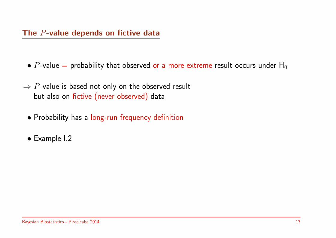
• P -value = probability that observed or a more extreme result occurs under H0
⇒ P -value = surprise index
• P -value = p(H0 | y)
• p(H0 | y) = Bayesian probability
Bayesian Biostatistics - Piracicaba 2014 16
The P -value depends on fictive data
• P -value = probability that observed or a more extreme result occurs under H0
⇒ P -value is based not only on the observed resultbut also on fictive (never observed) data
• Probability has a long-run frequency definition
• Example I.2
Bayesian Biostatistics - Piracicaba 2014 17

Example I.2: Graphical representation of P -value
P -value of RCT (Example I.1)
t
Density
4 2 0 2 4
0.0
0.1
0.2
0.3
0.4
0.015
area
0.015
area
observed t value
unobserved y values
Bayesian Biostatistics - Piracicaba 2014 18

The P -value depends on the sample space
• P -value = probability that observed or a more extreme result occurs if H0 is true
⇒ Calculation of P -value depends on all possible samples (under H0)
• The possible samples are similar in some characteristics to the observed sample(e.g. same sample size)
• Examples I.3 and I.4
Bayesian Biostatistics - Piracicaba 2014 19
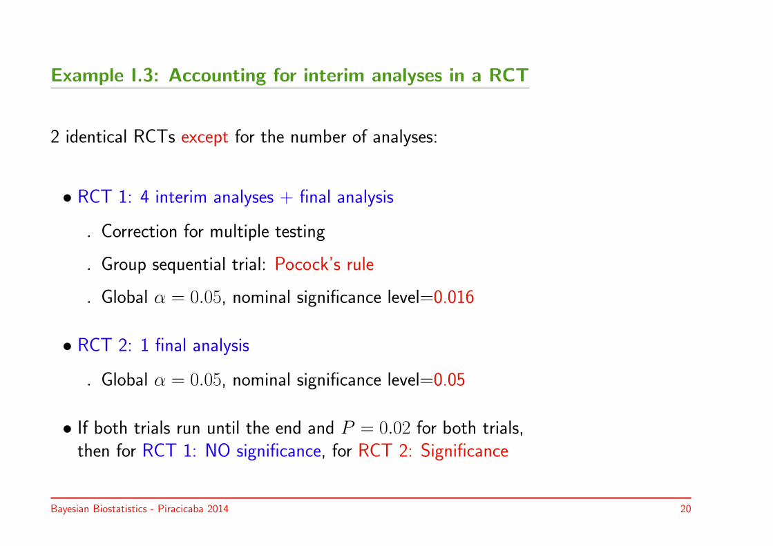
Example I.3: Accounting for interim analyses in a RCT
2 identical RCTs except for the number of analyses:
• RCT 1: 4 interim analyses + final analysis
◃ Correction for multiple testing
◃ Group sequential trial: Pocock’s rule
◃ Global α = 0.05, nominal significance level=0.016
• RCT 2: 1 final analysis
◃ Global α = 0.05, nominal significance level=0.05
• If both trials run until the end and P = 0.02 for both trials,then for RCT 1: NO significance, for RCT 2: Significance
Bayesian Biostatistics - Piracicaba 2014 20

Example I.4: Kaldor et al’s case-control study
• Case-control study (Kaldor et al., 1990) to examine the impact of chemotherapyon leukaemia in Hodgkin’s survivors
• 149 cases (leukaemia) and 411 controls
• Question: Does chemotherapy induce excess risk of developing solid tumors,leukaemia and/or lymphomas?
Treatment Controls Cases
No Chemo 160 11
Chemo 251 138
Total 411 149
Bayesian Biostatistics - Piracicaba 2014 21
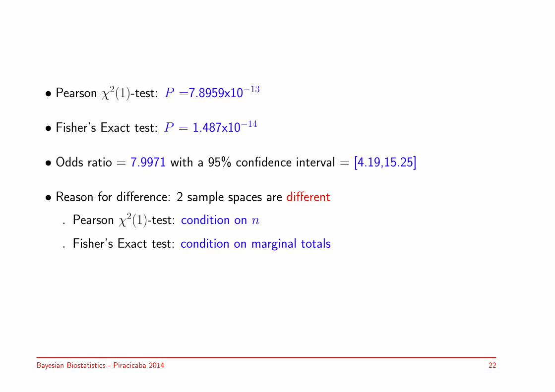
• Pearson χ2(1)-test: P =7.8959x10⁻¹³
• Fisher’s Exact test: P = 1.487x10⁻¹⁴
• Odds ratio = 7.9971 with a 95% confidence interval = [4.19,15.25]
• Reason for difference: 2 sample spaces are different
◃ Pearson χ2(1)-test: condition on n
◃ Fisher’s Exact test: condition on marginal totals
Bayesian Biostatistics - Piracicaba 2014 22

The P -value is not an absolute measure
• Small P -value does not necessarily indicate large difference between treatments,strong association, etc.
• Interpretation of a small P -value in a small/large study
Bayesian Biostatistics - Piracicaba 2014 23

The P -value does not take all evidence into account
• Studies are analyzed in isolation, no reference to historical data
• Why not incorporating past information in current study?
Bayesian Biostatistics - Piracicaba 2014 24

Example I.5: Merseyside registry results
• Subsequent registry study in UK
• Preliminary results of the Merseyside registry: P = 0.67
• Conclusion: no excess effect of chemotherapy (?)
Treatment Controls Cases
No Chemo 3 0
Chemo 3 2
Total 6 2
Bayesian Biostatistics - Piracicaba 2014 25

1.1.3 The confidence interval as a measure of evidence
• 95% confidence interval: expression of uncertainty on parameter of interest
• Technical definition: in 95 out of 100 studies true parameter is enclosed
• In each study confidence interval includes/does not include true value
• Practical interpretation has a Bayesian nature
Bayesian Biostatistics - Piracicaba 2014 26
Example I.6: 95% confidence interval toenail RCT
• 95% confidence interval for ∆ = [0.14, 2.62]
• Interpretation: most likely (with 0.95 probability) ∆ lies between 0.14 and 2.62
= a Bayesian interpretation
Bayesian Biostatistics - Piracicaba 2014 27

1.2 Statistical inference based on the likelihood function
• Inference purely on likelihood function has not been developed to a full-blownstatistical approach
• Considered here as a pre-cursor to Bayesian approach
• In the likelihood approach, one conditions on the observed data
Bayesian Biostatistics - Piracicaba 2014 28

1.2.1 The likelihood function
• Likelihood was introduced by Fisher in 1922
• Likelihood function = plausibility of the observed data as a function of theparameters of the stochastic model
• Inference based on likelihood function is QUITE different from inference based onP -value
Bayesian Biostatistics - Piracicaba 2014 29

Example I.7: A surgery experiment
• New but rather complicated surgical technique
• Surgeon operates n = 12 patients with s = 9 successes
• Notation:
◦ Result on ith operation: success yi = 1, failure yi = 0
◦ Total experiment: n operations with s successes
◦ Sample {y1, . . . , yn} ≡ y◦ Probability of success = p(yi) = θ
⇒ Binomial distribution:Expresses probability of s successes out of n experiments.
Bayesian Biostatistics - Piracicaba 2014 30

Binomial distribution
fθ (s) =
n
s
θs (1− θ)n−swith s =
n∑i=1
yi
• θ fixed & function of s:
fθ (s) is discrete distribution withn∑s=0
fθ (s) = 1
• s fixed & function of θ:
⇒ binomial likelihood function L(θ|s)
Bayesian Biostatistics - Piracicaba 2014 31
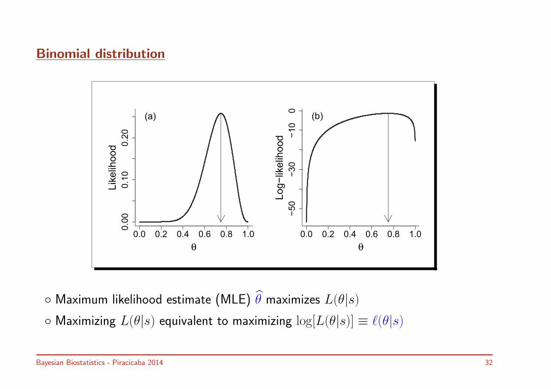
Binomial distribution
0.0 0.2 0.4 0.6 0.8 1.0
0.00
0.10
0.20
θ
Likelihood
(a)
0.0 0.2 0.4 0.6 0.8 1.0
−50
−30
−10
0
θ
Log−likelihood
(b)
◦ Maximum likelihood estimate (MLE) θ maximizes L(θ|s)◦ Maximizing L(θ|s) equivalent to maximizing log[L(θ|s)] ≡ ℓ(θ|s)
Bayesian Biostatistics - Piracicaba 2014 32
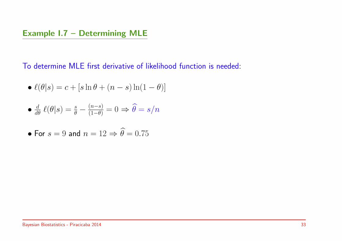
Example I.7 – Determining MLE
To determine MLE first derivative of likelihood function is needed:
• ℓ(θ|s) = c + [s ln θ + (n− s) ln(1− θ)]
• ddθ ℓ(θ|s) =
sθ −
(n−s)(1−θ) = 0 ⇒ θ = s/n
• For s = 9 and n = 12 ⇒ θ = 0.75
Bayesian Biostatistics - Piracicaba 2014 33

1.2.2 The likelihood principles
Two likelihood principles (LP):
• LP 1: All evidence, which is obtained from an experiment, about an unknownquantity θ, is contained in the likelihood function of θ for the given data ⇒
◃ Standardized likelihood
◃ Interval of evidence
• LP 2: Two likelihood functions for θ contain the same information about θ if theyare proportional to each other.
Bayesian Biostatistics - Piracicaba 2014 34

Likelihood principle 1
LP 1: All evidence, which is obtained from an experiment, about an unknown quantityθ, is contained in the likelihood function of θ for the given data
Bayesian Biostatistics - Piracicaba 2014 35

Example I.7 (continued)
• Maximal evidence for θ = 0.75
• Likelihood ratio L(0.5|s)/L(0.75|s) = relative evidence for 2 hypotheses θ = 0.5& θ = 0.75 (0.21 ⇒??)
• Standardized likelihood: LS(θ|s) ≡ L(θ|s)/L(θ|s)
• LS(0.5|s) = 0.21 = test for hypothesis H0 without involving fictive data
• Interval of (≥ 1/2 maximal) evidence
Bayesian Biostatistics - Piracicaba 2014 36

Inference on the likelihood function:
0.0 0.2 0.4 0.6 0.8 1.0
0.0
00.0
50.1
00.1
50.2
00.2
5
θ
Lik
elihood
Binomial likelihood
95% CI
MLE
interval of >= 1/2 evidence
Bayesian Biostatistics - Piracicaba 2014 37

Likelihood principle 2
LP 2: Two likelihood functions for θ contain the same information about θif they are proportional to each other
• LP 2 = Relative likelihood principle
⇒ When likelihood is proportional under two experimental conditions, theninformation about θ must be the same!
Bayesian Biostatistics - Piracicaba 2014 38

Example I.8: Another surgery experiment
◃ Surgeon 1: (Example I.7) Operates n = 12 patients, observes s = 9 successes(and 3 failures)
◃ Surgeon 2: Operates n patients until k = 3 failures are observed (n = s + k).And, suppose s = 9
◃ Surgeon 1: s =n∑i=1
yi has a binomial distribution
⇒ binomial likelihood L1(θ|s) =(ns
)θs(1− θ)(n−s)
◃ Surgeon 2: s =n∑i=1
yi has a negative binomial (Pascal) distribution
⇒ negative binomial likelihood L2(θ|s) =(s+k−1
s
)θs(1− θ)k
Bayesian Biostatistics - Piracicaba 2014 39

Inference on the likelihood function:
0.0 0.2 0.4 0.6 0.8 1.0
0.0
00.0
50.1
00.1
50.2
00.2
5
θ
Lik
elih
ood
Binomial likelihood
Negative binomial likelihood
MLE
interval of >= 1/2 evidence
LP 2: 2 experiments give us the same information about θ
Bayesian Biostatistics - Piracicaba 2014 40
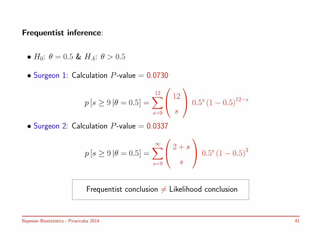
Frequentist inference:
• H0: θ = 0.5 & HA: θ > 0.5
• Surgeon 1: Calculation P -value = 0.0730
p [s ≥ 9 |θ = 0.5] =
12∑s=9
12
s
0.5s (1− 0.5)12−s
• Surgeon 2: Calculation P -value = 0.0337
p [s ≥ 9 |θ = 0.5] =
∞∑s=9
2 + s
s
0.5s (1− 0.5)3
Frequentist conclusion = Likelihood conclusion
Bayesian Biostatistics - Piracicaba 2014 41
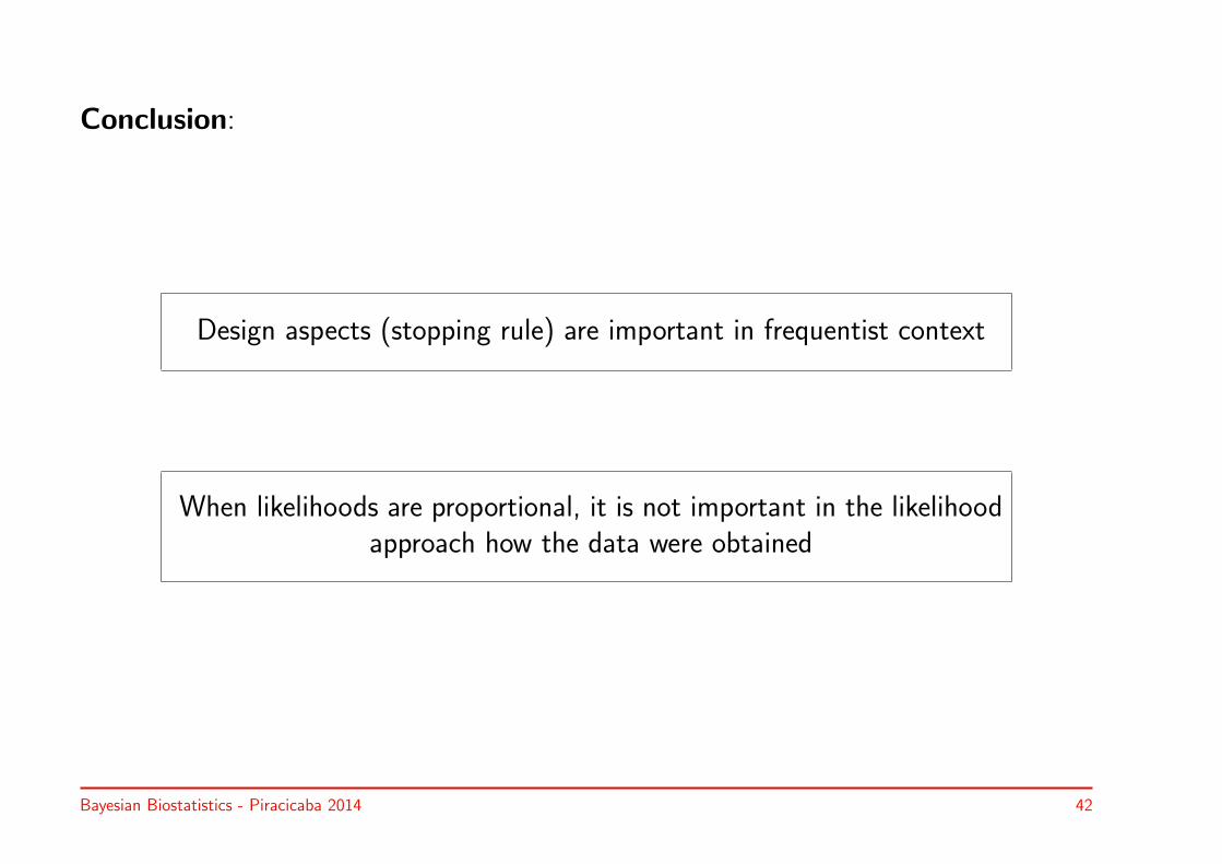
Conclusion:
Design aspects (stopping rule) are important in frequentist context
When likelihoods are proportional, it is not important in the likelihoodapproach how the data were obtained
Bayesian Biostatistics - Piracicaba 2014 42

1.3 The Bayesian approach: some basic ideas
• Bayesian methodology = topic of the course
• Statistical inference through different type of “glasses”
Bayesian Biostatistics - Piracicaba 2014 43

1.3.1 Introduction
• Examples I.7 and I.8: combination of information from a similar historical surgicaltechnique could be used in the evaluation of current technique = Bayesian exercise
• Planning phase III study:
◃ Comparison new ⇔ old treatment for treating breast cancer
◃ Background information is incorporated when writing the protocol
◃ Background information is not incorporated in the statistical analysis
◃ Suppose small-scaled study with unexpectedly positive result (P < 0.01)
⇒ Reaction???
Bayesian Biostatistics - Piracicaba 2014 44
• Medical device trials:
◃ The effect of a medical device is better understood than that of a drug
◃ It is very difficult to motivate surgeons to use concurrent controls to comparethe new device with the control device
◃ Can we capitalize on the information of the past to evaluate the performanceof the new device? Using only a single arm trial??
Bayesian Biostatistics - Piracicaba 2014 45
Central idea of Bayesian approach:
Combine likelihood (data) with Your priorknowledge (prior probability) to update informationon the parameter to result in a revised probability
associated with the parameter (posterior probability)
Bayesian Biostatistics - Piracicaba 2014 46
Example I.9: Examples of Bayesian reasoning in daily life
• Tourist example: Prior view on Belgians + visit to Belgium (data) ⇒ posteriorview on Belgians
• Marketing example: Launch of new energy drink on the market
• Medical example: Patients treated for CVA with thrombolytic agent suffer fromSBAs. Historical studies (20% - prior), pilot study (10% - data) ⇒ posterior
Bayesian Biostatistics - Piracicaba 2014 47
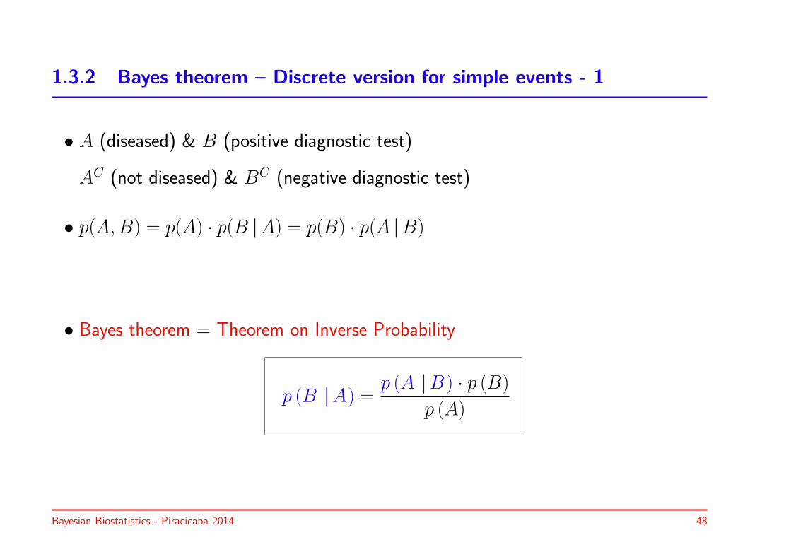
1.3.2 Bayes theorem – Discrete version for simple events - 1
• A (diseased) & B (positive diagnostic test)
AC (not diseased) & BC (negative diagnostic test)
• p(A,B) = p(A) · p(B |A) = p(B) · p(A |B)
• Bayes theorem = Theorem on Inverse Probability
p (B |A) =p (A |B ) · p (B)
p (A)
Bayesian Biostatistics - Piracicaba 2014 48
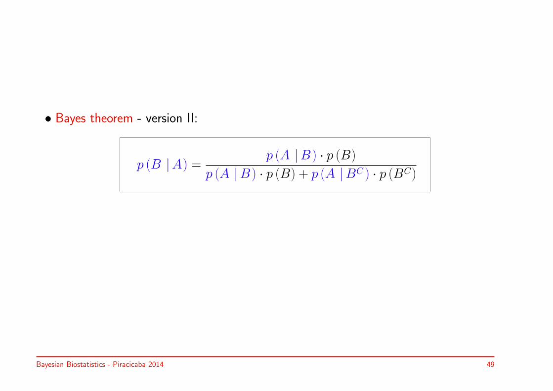
• Bayes theorem - version II:
p (B |A) =p (A |B ) · p (B)
p (A |B ) · p (B) + p (A |BC ) · p (BC)
Bayesian Biostatistics - Piracicaba 2014 49

Example I.10: Sensitivity, specificity, prevalence and predictive values
• B = “diseased”, A = “positive diagnostic test”
• Characteristics of diagnostic test:
◃ Sensitivity (Se) = p (A |B )
◃ Specificity (Sp) = p(AC
∣∣BC)
◃ Positive predictive value (pred+) = p (B |A)
◃ Negative predictive value (pred-) = p(BC
∣∣AC)
◃ Prevalence (prev) = p(B)
• pred+ calculated from Se, Sp and prev using Bayes theorem
Bayesian Biostatistics - Piracicaba 2014 50

• Folin-Wu blood test: screening test for diabetes (Boston City Hospital)
Test Diabetic Non-diabetic Total
+ 56 49 105
- 14 461 475
Total 70 510 580
◦ Se = 56/70 = 0.80
◦ Sp = 461/510 = 0.90
◦ prev = 70/580 = 0.12
Bayesian Biostatistics - Piracicaba 2014 51
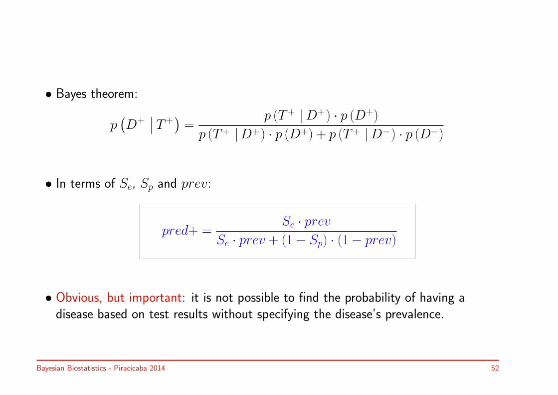
• Bayes theorem:
p(D+
∣∣T+)=
p (T+ |D+) · p (D+)
p (T+ |D+) · p (D+) + p (T+ |D−) · p (D−)
• In terms of Se, Sp and prev:
pred+ =Se · prev
Se · prev + (1− Sp) · (1− prev)
• Obvious, but important: it is not possible to find the probability of having adisease based on test results without specifying the disease’s prevalence.
Bayesian Biostatistics - Piracicaba 2014 52
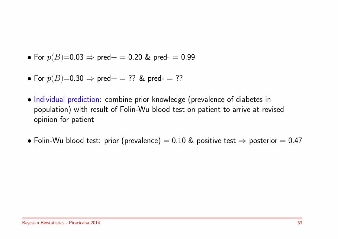
• For p(B)=0.03 ⇒ pred+ = 0.20 & pred- = 0.99
• For p(B)=0.30 ⇒ pred+ = ?? & pred- = ??
• Individual prediction: combine prior knowledge (prevalence of diabetes inpopulation) with result of Folin-Wu blood test on patient to arrive at revisedopinion for patient
• Folin-Wu blood test: prior (prevalence) = 0.10 & positive test ⇒ posterior = 0.47
Bayesian Biostatistics - Piracicaba 2014 53

1.4 Outlook
• Bayes theorem will be further developed in the next chapter ⇒ such that itbecomes useful in statistical practice
• Reanalyze examples such as those seen in this chapter
• Valid question: What can a Bayesian analysis do more than a classicalfrequentist analysis?
• Six additional chapters are needed to develop useful Bayesian tools
• But it is worth the effort!
Bayesian Biostatistics - Piracicaba 2014 54
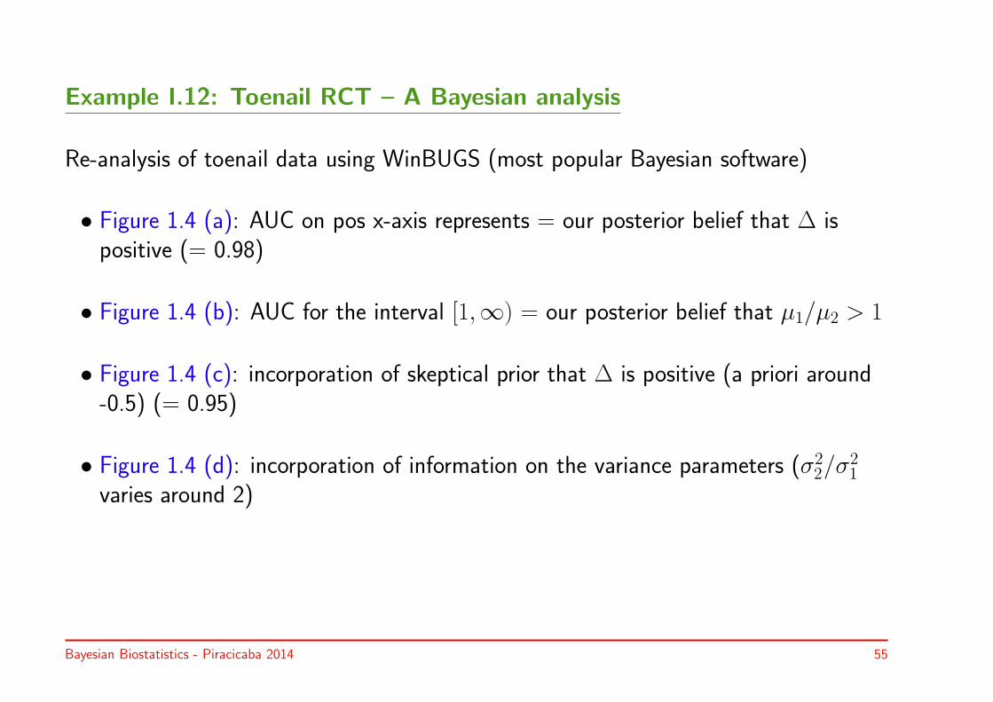
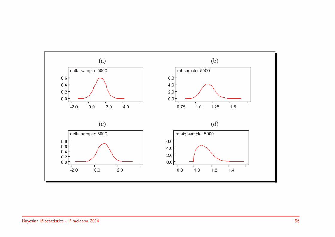
Example I.12: Toenail RCT – A Bayesian analysis
Re-analysis of toenail data using WinBUGS (most popular Bayesian software)
• Figure 1.4 (a): AUC on pos x-axis represents = our posterior belief that ∆ ispositive (= 0.98)
• Figure 1.4 (b): AUC for the interval [1,∞) = our posterior belief that µ1/µ2 > 1
• Figure 1.4 (c): incorporation of skeptical prior that ∆ is positive (a priori around-0.5) (= 0.95)
• Figure 1.4 (d): incorporation of information on the variance parameters (σ22/σ21
varies around 2)
Bayesian Biostatistics - Piracicaba 2014 55
(a) (b)
delta sample: 5000
-2.0 0.0 2.0 4.0
0.0
0.2
0.4
0.6
rat sample: 5000
0.75 1.0 1.25 1.5
0.0
2.0
4.0
6.0
(c) (d)
delta sample: 5000
-2.0 0.0 2.0
0.0
0.2
0.4
0.6
0.8
ratsig sample: 5000
0.8 1.0 1.2 1.4
0.0
2.0
4.0
6.0
Bayesian Biostatistics - Piracicaba 2014 56

True stories ...
A Bayesian and a frequentist were sentenced to death. When the judge asked whattheir final wishes were, the Bayesian replied that he wished to teach the frequentist theultimate lesson. The judge granted his request and then repeated the question to thefrequentist. He replied that he wished to get the lesson again and again and again . . .
A Bayesian is walking in the fields expecting to meet horses. However, suddenly he runsinto a donkey. Looks at the animal and continues his path concluding that he saw a
mule.
Bayesian Biostatistics - Piracicaba 2014 57

Take home messages
• The P -value does not bring the message as it is perceived by many, i.e. it is notthe probability that H0 is true or false
• The confidence interval is generally accepted as a better tool for inference, but weinterpret it in a Bayesian way
• There are other ways of statistical inference
• Pure likelihood inference = Bayesian inference without a prior
• Bayesian inference builds on likelihood inference by adding what is known of theproblem
Bayesian Biostatistics - Piracicaba 2014 58
Chapter 2
Bayes theorem: computing the posterior distribution
Aims:
◃ Derive the general expression of Bayes theorem
◃ Exemplify the computations
Bayesian Biostatistics - Piracicaba 2014 59
2.1 Introduction
In this chapter:
• Bayes theorem for binary outcomes, counts and continuous outcomes case
• Derivation of posterior distribution: for binomial, normal and Poisson
• A variety of examples
Bayesian Biostatistics - Piracicaba 2014 60

2.2 Bayes theorem – The binary version
◦ D+ ≡ θ = 1 and D− ≡ θ = 0 (diabetes)
◦ T+ ≡ y = 1 and T− ≡ y = 0 (Folin-Wu test)
p(θ = 1 | y = 1) =p(y = 1 | θ = 1) · p(θ = 1)
p(y = 1 | θ = 1) · p(θ = 1) + p(y = 1 | θ = 0) · p(θ = 0)
◦ p(θ = 1), p(θ = 0) prior probabilities
◦ p(y = 1 | θ = 1) likelihood
◦ p(θ = 1 | y = 1) posterior probability
⇒ Now parameter has also a probability
Bayesian Biostatistics - Piracicaba 2014 61
Bayes theorem
Shorthand notation
p(θ | y) = p(y | θ)p(θ)p(y)
where θ can stand for θ = 0 or θ = 1.
Bayesian Biostatistics - Piracicaba 2014 62

2.3 Probability in a Bayesian context
Bayesian probability = expression of Our/Your uncertainty of the parameter value
• Coin tossing: truth is there, but unknown to us
• Diabetes: from population to individual patient
Probability can have two meanings: limiting proportion (objective) or personal belief(subjective)
Bayesian Biostatistics - Piracicaba 2014 63
Other examples of Bayesian probabilities
Subjective probability varies with individual, in time, etc.
• Tour de France
• FIFA World Cup 2014
• Global warming
• . . .
Bayesian Biostatistics - Piracicaba 2014 64
Subjective probability rules
Let A1, A2, . . . , AK mutually exclusive events with total event S
Subjective probability p should be coherent:
• Ak: p(Ak) ≥ 0 (k=1, . . ., K)
• p(S) = 1
• p(AC) = 1− p(A)
• With B1, B2, . . . , BL another set of mutually exclusive events:
p(Ai | Bj) =p(Ai, Bj)
p(Bj)
Bayesian Biostatistics - Piracicaba 2014 65
2.4 Bayes theorem – The categorical version
• Subject can belong to K > 2 classes: θ1, θ2, . . . , θK
• y takes L different values: y1, . . . , yL or continuous
⇒ Bayes theorem for categorical parameter:
p (θk | y) =p (y | θk) p (θk)K∑k=1
p (y | θk) p (θk)
Bayesian Biostatistics - Piracicaba 2014 66
2.5 Bayes theorem – The continuous version
• 1-dimensional continuous parameter θ
• i.i.d. sample y = y1, . . . , yn
• Joint distribution of sample = p(y|θ) =∏n
i=1 p(yi|θ) = likelihood L(θ|y)
• Prior density function p(θ)
• Split up: p(y, θ) = p(y|θ)p(θ) = p(θ|y)p(y)
⇒ Bayes theorem for continuous parameters:
p(θ|y) = L(θ|y)p(θ)p(y)
=L(θ|y)p(θ)∫L(θ|y)p(θ)dθ
Bayesian Biostatistics - Piracicaba 2014 67

• Shorter: p(θ|y) ∝ L(θ|y)p(θ)
•∫L(θ|y)p(θ)dθ = averaged likelihood
• Averaged likelihood ⇒ posterior distribution involves integration
• θ is now a random variable and is described by a probability distribution. Allbecause we express our uncertainty on the parameter
• In the Bayesian approach (as in likelihood approach), one only looks at theobserved data. No fictive data are involved
• One says: In the Bayesian approach, one conditions on the observed data. Inother words, the data are fixed and p(y) is a constant!
Bayesian Biostatistics - Piracicaba 2014 68

2.6 The binomial case
Example II.1: Stroke study – Monitoring safety
◃ Rt-PA: thrombolytic for ischemic stroke
◃ Historical studies ECASS 1 and ECASS 2: complication SICH
◃ ECASS 3 study: patients with ischemic stroke (Tx between 3 & 4.5 hours)
◃ DSMB: monitor SICH in ECASS 3
◃ Fictive situation:
◦ First interim analysis ECASS 3: 50 rt-PA patients with 10 SICHs
◦ Historical data ECASS 2: 100 rt-PA patients with 8 SICHs
◃ Estimate risk for SICH in ECASS 3 ⇒ construct Bayesian stopping rule
Bayesian Biostatistics - Piracicaba 2014 69
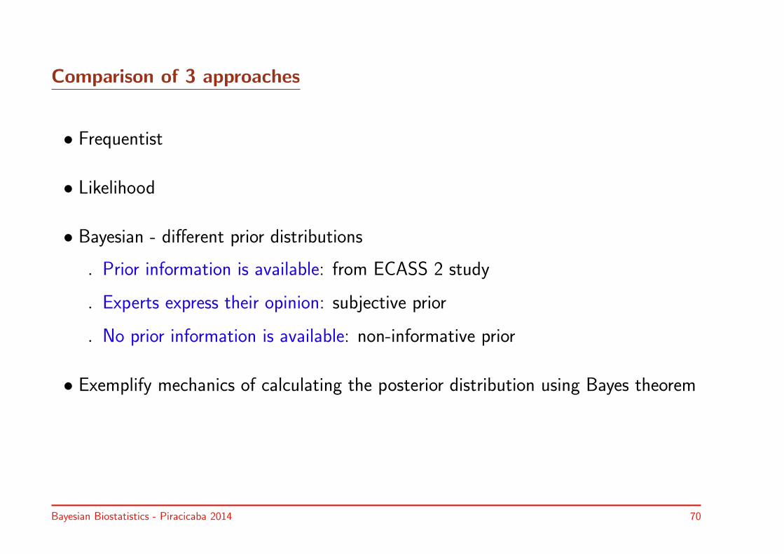
Comparison of 3 approaches
• Frequentist
• Likelihood
• Bayesian - different prior distributions
◃ Prior information is available: from ECASS 2 study
◃ Experts express their opinion: subjective prior
◃ No prior information is available: non-informative prior
• Exemplify mechanics of calculating the posterior distribution using Bayes theorem
Bayesian Biostatistics - Piracicaba 2014 70

Notation
• SICH incidence: θ
• i.i.d. Bernoulli random variables y1, . . . , yn
• SICH: yi = 1, otherwise yi = 0
• y =∑n
1 yi has Bin(n, θ): p(y|θ) =(ny
)θy(1− θ)(n−y)
Bayesian Biostatistics - Piracicaba 2014 71

Frequentist approach
• MLE θ = y/n = 10/50 = 0.20
• Test hypothesis θ = 0.08 with binomial test (8% = value of ECASS 2 study)
• Classical 95% confidence interval = [0.089, 0.31]
Bayesian Biostatistics - Piracicaba 2014 72
Likelihood inference
• MLE θ = 0.20
• No hypothesis test is performed
• 0.95 interval of evidence = [0.09, 0.36]
Bayesian Biostatistics - Piracicaba 2014 73

Bayesian approach: prior obtained from ECASS 2 study
1. Specifying the (ECASS 2) prior distribution
2. Constructing the posterior distribution
3. Characteristics of the posterior distribution
4. Equivalence of prior information and extra data
Bayesian Biostatistics - Piracicaba 2014 74

1. Specifying the (ECASS 2) prior distribution
• ECASS 2 likelihood: L(θ|y0) =(n0y0
)θy0(1− θ)(n0−y0) (y0 = 8 & n0 = 100)
• ECASS 2 likelihood expresses prior belief on θbut is not (yet) prior distribution
• As a function of θL(θ|y0) = density (AUC = 1)
• How to standardize?Numerically or analytically?
(a)
PROPORTION SICH
0.0 0.05 0.10 0.15 0.20 0.25 0.30
0.0
0.0
50.1
00.1
5
LIKELIHOOD
Bayesian Biostatistics - Piracicaba 2014 75

• Kernel of binomial likelihood θy0(1− θ)(n0−y0) ∝ beta density Beta(α, β):
p(θ) = 1B(α0,β0)
θα0−1(1− θ)β0−1
with B(α, β) = Γ(α)Γ(β)Γ(α+β)
Γ(·) gamma function
• α0(= 9) ≡ y0 + 1
β0(= 100− 8 + 1) ≡ n0 − y0 + 1
(b)
PROPORTION SICH
0.0 0.05 0.10 0.15 0.20 0.25 0.30
05
10
15
proportional to LIKELIHOOD
LIKELIHOOD
Bayesian Biostatistics - Piracicaba 2014 76
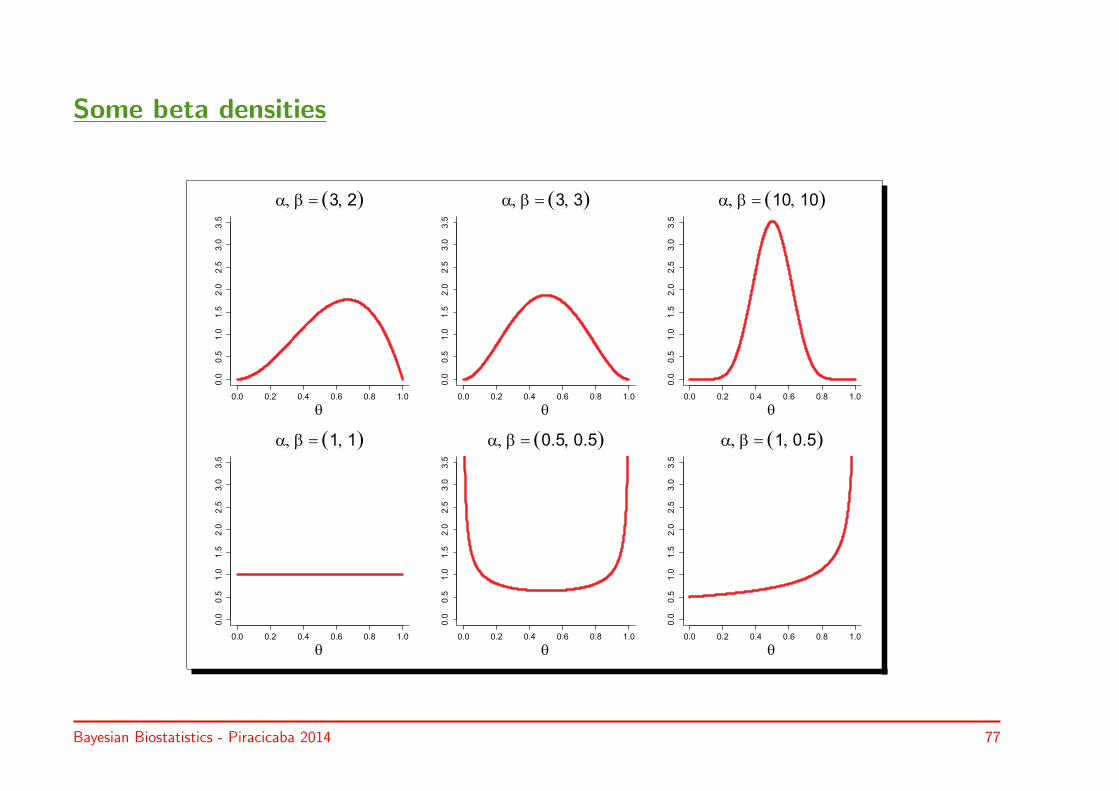
Some beta densities
��� ��� ��� ��� ��� ���
���
���
���
���
���
���
��
��
���� � �����
���� ��� ��� ��� ��� ���
���
���
���
���
���
���
��
��
���� � ����
���� ��� ��� ��� ��� ���
���
���
���
���
���
���
��
��
���� � ��������
�
��� ��� ��� ��� ��� ���
���
���
���
���
���
���
��
��
���� � ������
���� ��� ��� ��� ��� ���
���
���
���
���
���
���
��
��
���� � ����������
���� ��� ��� ��� ��� ���
���
���
���
���
���
���
��
��
���� � ��������
�
Bayesian Biostatistics - Piracicaba 2014 77

2. Constructing the posterior distribution
• Bayes theorem needs:
◃ Prior p(θ) (ECASS 2 study)
◃ Likelihood L(θ|y) (ECASS 3 interim analysis), y=10 & n=50
◃ Averaged likelihood∫L(θ|y)p(θ)dθ
• Numerator of Bayes theorem
L(θ|y) p(θ) =(n
y
)1
B(α0, β0)θα0+y−1(1− θ)β0+n−y−1
• Denominator of Bayes theorem = averaged likelihood
p(y) =
∫L(θ|y) p(θ) dθ =
(n
y
)B(α0 + y, β0 + n− y)
B(α0, β0)
Bayesian Biostatistics - Piracicaba 2014 78
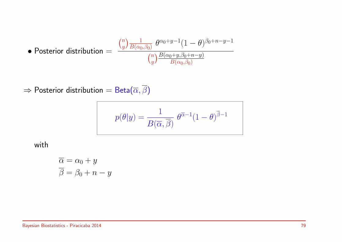
• Posterior distribution =
(ny
)1
B(α0,β0)θα0+y−1(1− θ)β0+n−y−1(
ny
)B(α0+y,β0+n−y)B(α0,β0)
⇒ Posterior distribution = Beta(α, β)
p(θ|y) = 1
B(α, β)θα−1(1− θ)β−1
with
α = α0 + y
β = β0 + n− y
Bayesian Biostatistics - Piracicaba 2014 79

2. Prior, likelihood & posterior
0.0 0.1 0.2 0.3 0.4
05
10
15
θ
Prior
θ0
Proportional to
likelihood
θ^
Posterior
θ^
M
Bayesian Biostatistics - Piracicaba 2014 80
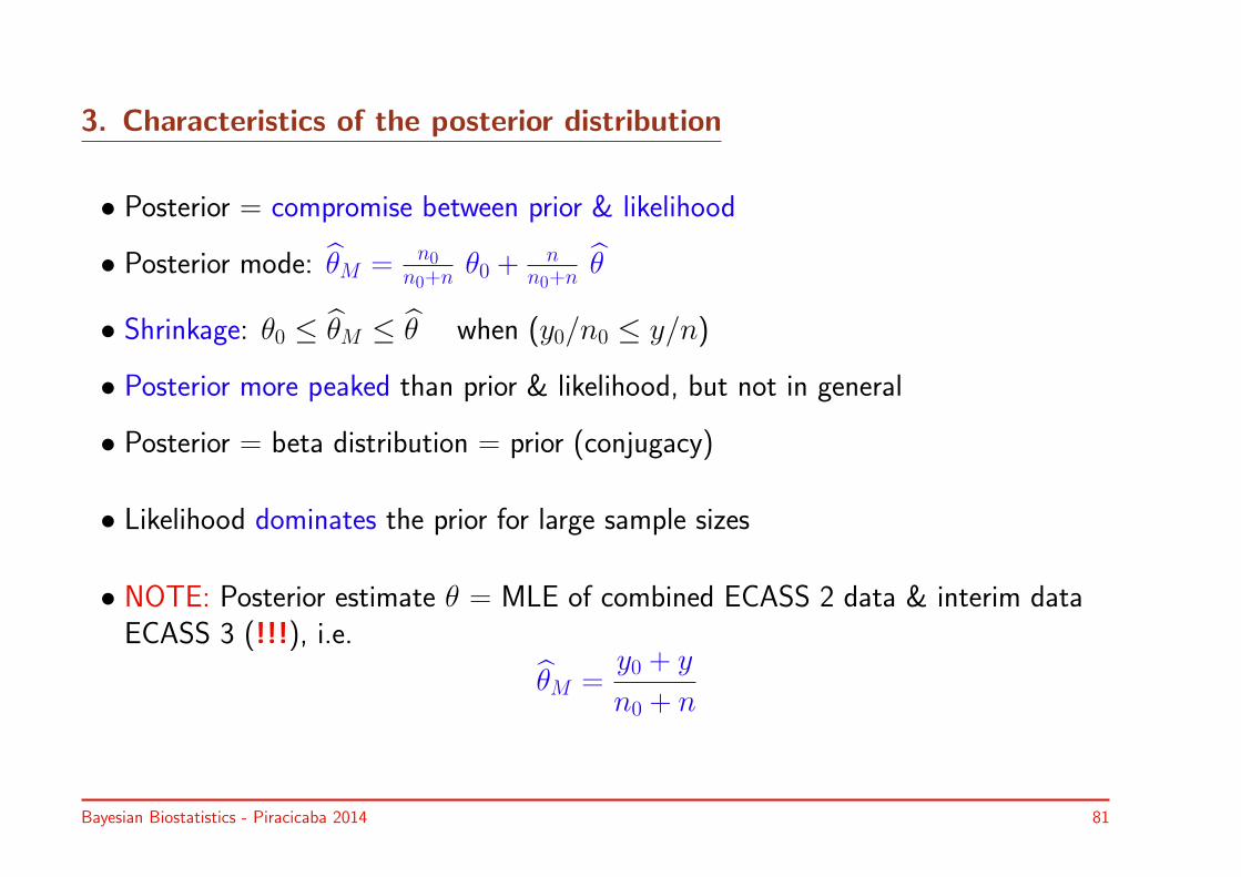
3. Characteristics of the posterior distribution
• Posterior = compromise between prior & likelihood
• Posterior mode: θM = n0n0+n
θ0 +n
n0+nθ
• Shrinkage: θ0 ≤ θM ≤ θ when (y0/n0 ≤ y/n)
• Posterior more peaked than prior & likelihood, but not in general
• Posterior = beta distribution = prior (conjugacy)
• Likelihood dominates the prior for large sample sizes
• NOTE: Posterior estimate θ = MLE of combined ECASS 2 data & interim dataECASS 3 (!!!), i.e.
θM =y0 + y
n0 + n
Bayesian Biostatistics - Piracicaba 2014 81

Example dominance of likelihood
0.0 0.2 0.4 0.6 0.8 1.0
020
40
60
80
θ
POSTERIOR
PRIOR 1
0.0 0.2 0.4 0.6 0.8 1.0
020
40
60
80
θ
POSTERIOR
PRIOR 2
0.0 0.2 0.4 0.6 0.8 1.0
020
40
60
80
θ
POSTERIOR
PRIOR 3
0.0 0.2 0.4 0.6 0.8 1.0
020
40
60
80
θ
POSTERIOR
PRIOR 4
Likelihood based on 5,000 subjects with 800 “successes”
Bayesian Biostatistics - Piracicaba 2014 82
4. Equivalence of prior information and extra data
• Beta(α0, β0) prior
≡ binomial experiment with (α0− 1) successes in (α0+ β0− 2) experiments
⇒ Prior
≈ extra data to observed data set: (α0 − 1) successes and (β0 − 1) failures
Bayesian Biostatistics - Piracicaba 2014 83
Bayesian approach: using a subjective prior
• Suppose DSMB neurologists ‘believe’ that SICH incidence is probably more than5% but most likely not more than 20%
• If prior belief = ECASS 2 prior density ⇒ posterior inference is the same
• The neurologists could also combine their qualitative prior belief with ECASS 2data to construct a prior distribution ⇒ adjust ECASS 2 prior
Bayesian Biostatistics - Piracicaba 2014 84

Example subjective prior
0.0 0.1 0.2 0.3 0.4
05
10
15
θ
ECASS 2
PRIOR
ECASS 2
POSTERIOR
SUBJECTIVE
PRIOR
SUBJECTIVE
POSTERIOR
Bayesian Biostatistics - Piracicaba 2014 85
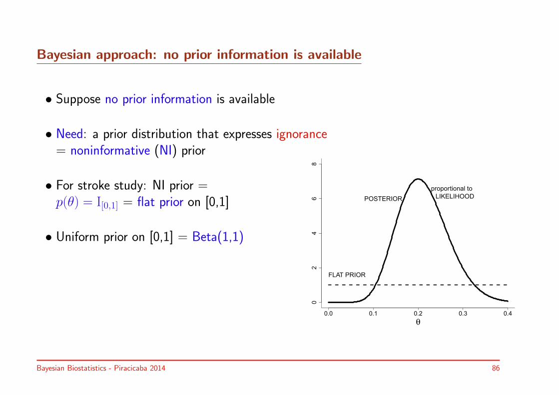
Bayesian approach: no prior information is available
• Suppose no prior information is available
• Need: a prior distribution that expresses ignorance= noninformative (NI) prior
• For stroke study: NI prior =p(θ) = I[0,1] = flat prior on [0,1]
• Uniform prior on [0,1] = Beta(1,1)
0.0 0.1 0.2 0.3 0.40
24
68
θ
FLAT PRIOR
proportional to
LIKELIHOODPOSTERIOR
Bayesian Biostatistics - Piracicaba 2014 86
2.7 The Gaussian case
Example II.2: Dietary study – Monitoring dietary behavior in Belgium
• IBBENS study: dietary survey in Belgium
• Of interest: intake of cholesterol
• Monitoring dietary behavior in Belgium: IBBENS-2 study
Assume σ is known
Bayesian Biostatistics - Piracicaba 2014 87
Bayesian approach: prior obtained from the IBBENS study
1. Specifying the (IBBENS) prior distribution
2. Constructing the posterior distribution
3. Characteristics of the posterior distribution
4. Equivalence of prior information and extra data
Bayesian Biostatistics - Piracicaba 2014 88

1. Specifying the (IBBENS) prior distribution
Histogram of the dietary cholesterol of 563 bank employees ≈ normal
• y ∼ N(µ, σ2) when
f (y) =1√2π σ
exp[−(y − µ)2/2σ2
]
• Sample y1, . . . , yn ⇒ likelihood
L(µ|y) ∝ exp
[− 1
2σ2
n∑i=1
(yi − µ)2
]∝ exp
[−1
2
(µ− y
σ/√n
)2]≡ L(µ|y)
Bayesian Biostatistics - Piracicaba 2014 89
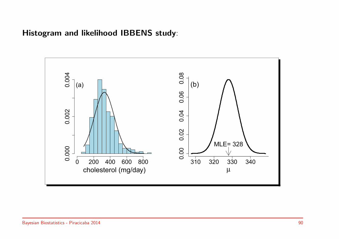
Histogram and likelihood IBBENS study:
cholesterol (mg/day)
0 200 400 600 800
0.0
00
0.0
02
0.0
04
(a)
310 320 330 340
0.0
00.0
20.0
40.0
60.0
8
µ
(b)
MLE= 328
Bayesian Biostatistics - Piracicaba 2014 90
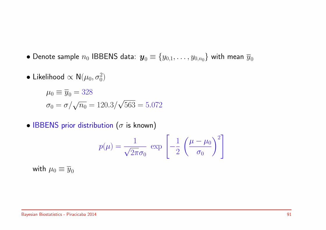
• Denote sample n0 IBBENS data: y0 ≡ {y0,1, . . . , y0,n0} with mean y0
• Likelihood ∝ N(µ0, σ20)
µ0 ≡ y0 = 328
σ0 = σ/√n0 = 120.3/
√563 = 5.072
• IBBENS prior distribution (σ is known)
p(µ) =1√2πσ0
exp
[−1
2
(µ− µ0σ0
)2]
with µ0 ≡ y0
Bayesian Biostatistics - Piracicaba 2014 91
2. Constructing the posterior distribution
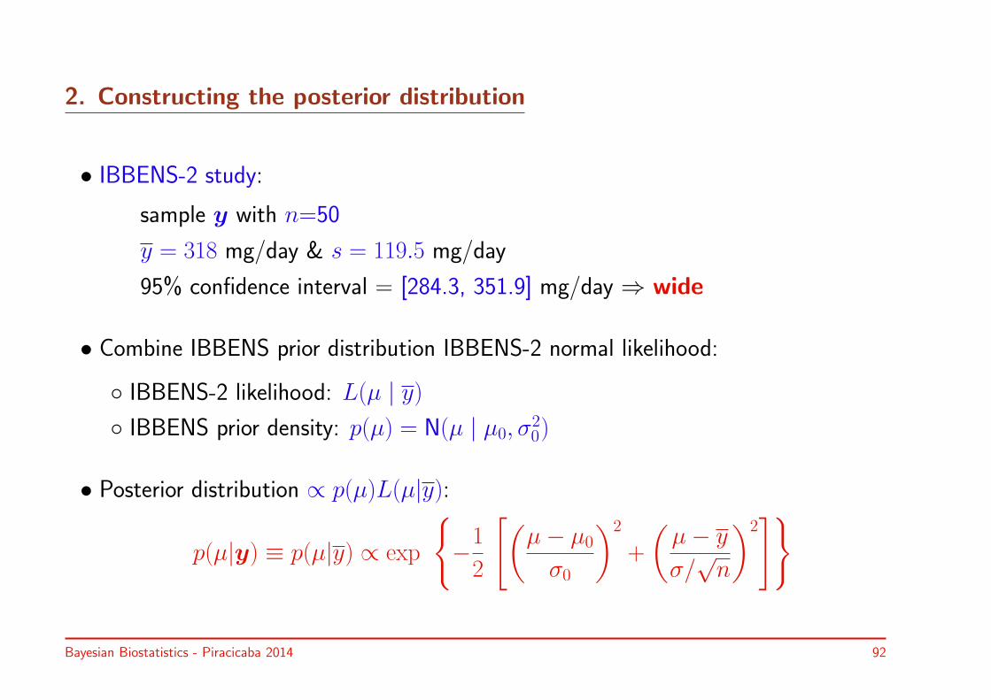
• IBBENS-2 study:
sample y with n=50
y = 318 mg/day & s = 119.5 mg/day
95% confidence interval = [284.3, 351.9] mg/day ⇒ wide
• Combine IBBENS prior distribution IBBENS-2 normal likelihood:
◦ IBBENS-2 likelihood: L(µ | y)◦ IBBENS prior density: p(µ) = N(µ | µ0, σ2
0)
• Posterior distribution ∝ p(µ)L(µ|y):
p(µ|y) ≡ p(µ|y) ∝ exp
{−1
2
[(µ− µ0σ0
)2
+
(µ− y
σ/√n
)2]}
Bayesian Biostatistics - Piracicaba 2014 92

◃ Integration constant to obtain density?
◃ Recognize standard distribution: exponent (quadratic function of µ)
◃ Posterior distribution:
p(µ|y) = N(µ, σ2),
with
µ =
1σ20µ0 +
nσ2y
1σ20+ n
σ2
and σ2 =1
1σ20+ n
σ2
◃ Here: µ = 327.2 and σ = 4.79.
Bayesian Biostatistics - Piracicaba 2014 93

IBBENS-2 posterior distribution:
250 300 350 400
0.0
00.0
20.0
40.0
60.0
8
µ
IBBENS PRIOR
IBBENS−2 LIKELIHOOD
IBBENS−2 POSTERIOR
Bayesian Biostatistics - Piracicaba 2014 94

3. Characteristics of the posterior distribution
◃ Posterior distribution: compromise between prior and likelihood
◃ Posterior mean: weighted average of prior and the sample mean
µ =w0
w0 + w1µ0 +
w1
w0 + w1y
with
w0 =1
σ20& w1 =
1
σ2/n
◃ The posterior precision = 1/posterior variance:
1
σ2= w0 + w1
with w0 = 1/σ20 = prior precision and w1 = 1/(σ2/n) = sample precision
Bayesian Biostatistics - Piracicaba 2014 95

• Posterior is always more peaked than prior and likelihood
• When n→ ∞ or σ0 → ∞: p(µ|y) = N(y, σ2/n)
⇒ When sample size increases the likelihood dominates the prior
• Posterior = normal = prior ⇒ conjugacy
Bayesian Biostatistics - Piracicaba 2014 96

4. Equivalence of prior information and extra data
• Prior variance σ20 = σ2 (unit information prior) ⇒ σ2 = σ2/(n + 1)
⇒ Prior information = adding one extra observation to the sample
• General: σ20 = σ2/n0, with n0 general
µ =n0
n0 + nµ0 +
n
n0 + ny
and
σ2 =σ2
n0 + n
Bayesian Biostatistics - Piracicaba 2014 97

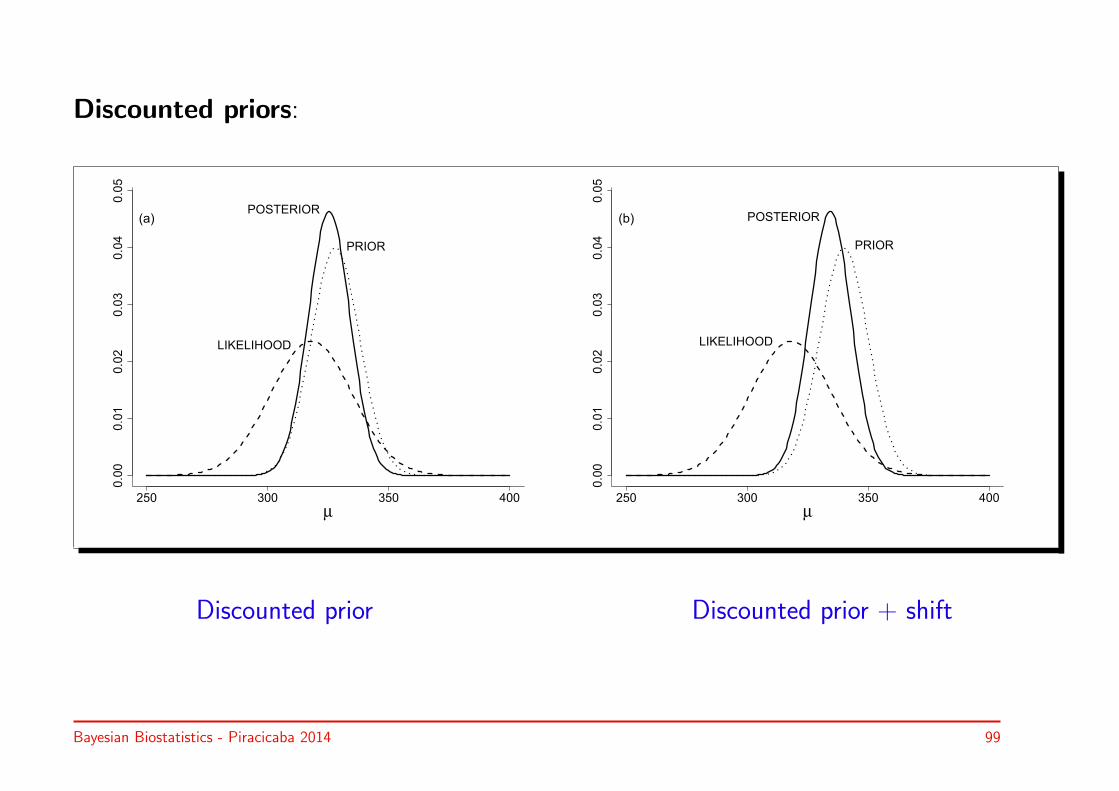
Bayesian approach: using a subjective prior
• Discounted IBBENS prior: increase IBBENS prior variance from 25 to 100
• Discounted IBBENS prior + shift: increase from µ0 = 328 to µ0 = 340
Bayesian Biostatistics - Piracicaba 2014 98
Discounted priors:
250 300 350 400
0.00
0.01
0.02
0.03
0.04
0.05
µ
PRIOR
LIKELIHOOD
POSTERIOR(a)
250 300 350 400
0.00
0.01
0.02
0.03
0.04
0.05
µ
PRIOR
LIKELIHOOD
POSTERIOR(b)
Discounted prior Discounted prior + shift
Bayesian Biostatistics - Piracicaba 2014 99

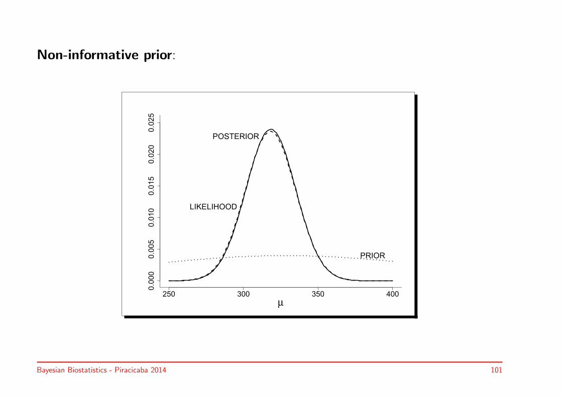
Bayesian approach: no prior information is available
• Non-informative prior: σ20 → ∞
⇒ Posterior: N(y, σ2/n)
Bayesian Biostatistics - Piracicaba 2014 100
Non-informative prior:
250 300 350 400
0.000
0.005
0.010
0.015
0.020
0.025
µ
PRIOR
LIKELIHOOD
POSTERIOR
Bayesian Biostatistics - Piracicaba 2014 101

2.8 The Poisson case
• Take y ≡ {y1, . . . , yn} independent counts ⇒ Poisson distribution
• Poisson(θ)p(y| θ) = θy e−θ
y!
• Mean and variance = θ
• Poisson likelihood:
L(θ|y) ≡n∏i=1
p(yi| θ) =n∏i=1
(θyi/yi!) e−nθ
Bayesian Biostatistics - Piracicaba 2014 102

Example II.6: Describing caries experience in Flanders
The Signal-Tandmobielr (STM) study:
• Longitudinal oral health study in Flanders
• Annual examinations from 1996 to 2001
• 4468 children (7% of children born in 1989)
• Caries experience measured by dmft-index(min=0, max=20)
0 5 10 15
0.0
0.1
0.2
0.3
0.4
dmft-index
PR
OP
OR
TIO
N
Bayesian Biostatistics - Piracicaba 2014 103

Frequentist and likelihood calculations
• MLE of θ: θ = y = 2.24
• Likelihood-based 95% confidence interval for θ: [2.1984,2.2875]
Bayesian Biostatistics - Piracicaba 2014 104

Bayesian approach: prior distribution based on historical data
1. Specifying the prior distribution
2. Constructing the posterior distribution
3. Characteristics of the posterior distribution
4. Equivalence of prior information and extra data
Bayesian Biostatistics - Piracicaba 2014 105

1. Specifying the prior distribution
• Information from literature:
◦ Average dmft-index 4.1 (Liege, 1983) & 1.39 (Gent, 1994)
◦ Oral hygiene has improved considerably in Flanders
◦ Average dmft-index bounded above by 10
• Candidate for prior: Gamma(α0, β0)
p(θ) =βα00Γ(α0)
θα0−1 e−β0θ
◦ α0 = shape parameter & β0 = inverse of scale parameter
◦ E(θ) = α0/β0 & var(θ) = α0/β20
• STM study: α0 = 3 & β0 = 1
Bayesian Biostatistics - Piracicaba 2014 106

Gamma prior for STM study:
0 5 10 15 20
0.00
0.05
0.10
0.15
0.20
0.25
θ
Gamma(3,1)
Bayesian Biostatistics - Piracicaba 2014 107

Some gamma densities
� � � � � ��
���
���
���
���
���
���
���� � ������
�� � � � � ��
���
���
���
���
���
���
���� � ������
�� � � � � ��
���
���
���
���
���
���
���� � ����
�
� � � � � ��
���
���
���
���
���
���
���� � ������
�� � � � � ��
���
���
���
���
���
���
���� � ����������
�� � � � � ��
���
���
���
���
���
���
���� � �������
�
Bayesian Biostatistics - Piracicaba 2014 108
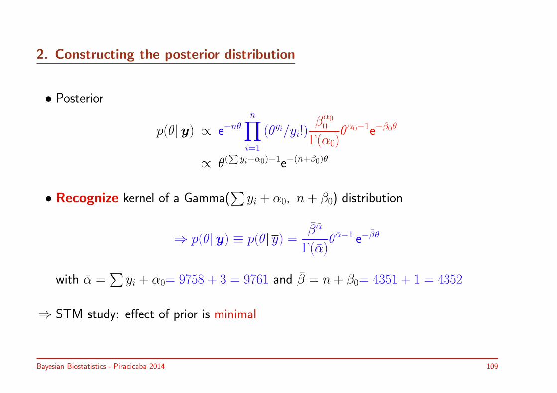
2. Constructing the posterior distribution
• Posterior
p(θ|y) ∝ e−nθn∏i=1
(θyi/yi!)βα00Γ(α0)
θα0−1e−β0θ
∝ θ(∑yi+α0)−1e−(n+β0)θ
• Recognize kernel of a Gamma(∑yi + α0, n + β0) distribution
⇒ p(θ|y) ≡ p(θ| y) = βα
Γ(α)θα−1 e−βθ
with α =∑yi + α0= 9758 + 3 = 9761 and β = n + β0= 4351 + 1 = 4352
⇒ STM study: effect of prior is minimal
Bayesian Biostatistics - Piracicaba 2014 109
3. Characteristics of the posterior distribution
• Posterior is a compromise between prior and likelihood
• Posterior mode demonstrates shrinkage
• For STM study posterior more peaked than prior likelihood, but not in general
• Prior is dominated by likelihood for a large sample size
• Posterior = gamma = prior ⇒ conjugacy
Bayesian Biostatistics - Piracicaba 2014 110

4. Equivalence of prior information and extra data
• Prior = equivalent to experiment of size β0 with counts summing up to α0 − 1
• STM study: prior corresponds to an experiment of size 1 with count equal to 2
Bayesian Biostatistics - Piracicaba 2014 111
Bayesian approach: no prior information is available
• Gamma with α0 ≈ 1 and β0 ≈ 0 = non-informative prior
Bayesian Biostatistics - Piracicaba 2014 112

2.9 The prior and posterior of derived parameter
• If p(θ) is prior of θ, what is then corresponding prior for h(θ) = ψ?
◃ Same question for posterior density
◃ Example: θ = odds ratio, ψ = log (odds ratio)
• Why do we wish to know this?
◃ Prior: prior information on θ and ψ should be the same
◃ Posterior: allows to reformulate conclusion on a different scale
• Solution: apply transformation rule p(h−1(ψ))(∣∣∣dh−1(ψ)
dψ
∣∣∣)• Note: parameter is a random variable!
Bayesian Biostatistics - Piracicaba 2014 113

Example II.4: Stroke study – Posterior distribution of log(θ)
• Probability of ‘success’ is often modeled on the log-scale (or logit scale)
• Posterior distribution of ψ = log(θ)
p(ψ|y) = 1
B(α, β)expψα(1− expψ)β−1
with α = 19 and β = 133.
Bayesian Biostatistics - Piracicaba 2014 114

Posterior and transformed posterior:
0.0 0.2 0.4 0.6 0.8 1.0
05
10
15
θ
PO
ST
ER
IOR
DE
NS
ITY
−4 −3 −2 −1 00.0
0.5
1.0
1.5
ψ
PO
ST
ER
IOR
DE
NS
ITY
Bayesian Biostatistics - Piracicaba 2014 115
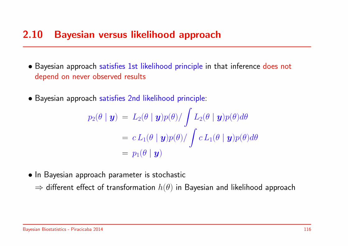
2.10 Bayesian versus likelihood approach
• Bayesian approach satisfies 1st likelihood principle in that inference does notdepend on never observed results
• Bayesian approach satisfies 2nd likelihood principle:
p2(θ | y) = L2(θ | y)p(θ)/∫L2(θ | y)p(θ)dθ
= c L1(θ | y)p(θ)/∫c L1(θ | y)p(θ)dθ
= p1(θ | y)
• In Bayesian approach parameter is stochastic
⇒ different effect of transformation h(θ) in Bayesian and likelihood approach
Bayesian Biostatistics - Piracicaba 2014 116
2.11 Bayesian versus frequentist approach
• Frequentist approach:
◃ θ fixed and data are stochastic
◃ Many tests are based on asymptotic arguments
◃ Maximization is key tool
◃ Does depend on stopping rules
• Bayesian approach:
◃ Condition on observed data (data fixed), uncertainty about θ (θ stochastic)
◃ No asymptotic arguments are needed, all inference depends on posterior
◃ Integration is key tool
◃ Does not depend on stopping rules
Bayesian Biostatistics - Piracicaba 2014 117

• Frequentist and Bayesian approach can give the same numerical output (withdifferent interpretation), but may give quite a different inference
• Frequentist ideas in Bayesian approaches (MCMC)
Bayesian Biostatistics - Piracicaba 2014 118

2.12 The different modes of the Bayesian approach
• Subjectivity ⇔ objectivity
• Subjective (proper) Bayesian ⇔ objective (reference) Bayesian
• Empirical Bayesian
• Decision-theoretic (full) Bayesian: use of utility function
• 46656 varieties of Bayesians (De Groot)
• Pragmatic Bayesian = Bayesian ??
Bayesian Biostatistics - Piracicaba 2014 119
2.13 An historical note on the Bayesian approach
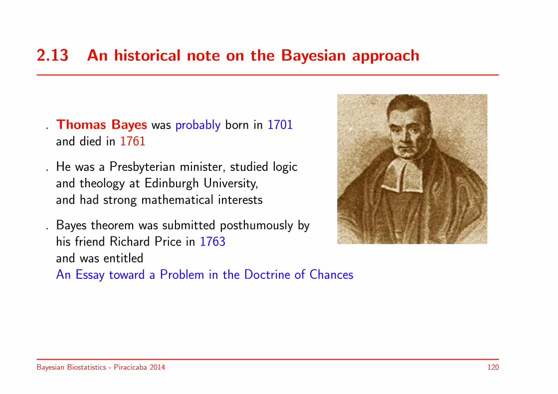
◃ Thomas Bayes was probably born in 1701and died in 1761
◃ He was a Presbyterian minister, studied logicand theology at Edinburgh University,and had strong mathematical interests
◃ Bayes theorem was submitted posthumously byhis friend Richard Price in 1763and was entitledAn Essay toward a Problem in the Doctrine of Chances
born on 1701 and died on 7-4-1761.
He was a minister and a reverent with mathematical interests.
None of his work on mathematics was published during his life.
Bayesian Biostatistics - Piracicaba 2014 120

◃ Up to 1950 Bayes theorem was calledTheorem of Inverse Probability
◃ Fundament of Bayesian theory was developed byPierre-Simon Laplace (1749-827)
◃ Laplace first assumed indifference prior,later he relaxed this assumption
◃ Much opposition:e.g. Poisson, Fisher, Neyman and Pearson, etc
Bayesian Biostatistics - Piracicaba 2014 121
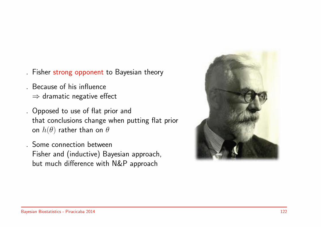
◃ Fisher strong opponent to Bayesian theory
◃ Because of his influence⇒ dramatic negative effect
◃ Opposed to use of flat prior andthat conclusions change when putting flat prioron h(θ) rather than on θ
◃ Some connection betweenFisher and (inductive) Bayesian approach,but much difference with N&P approach
Bayesian Biostatistics - Piracicaba 2014 122

Proponents of the Bayesian approach:
• de Finetti: exchangeability
• Jeffreys: noninformative prior, Bayes factor
• Savage: theory of subjective and personal probability and statistics
• Lindley: Gaussian hierarchical models
• Geman & Geman: Gibbs sampling
• Gelfand & Smith: introduction of Gibbs sampling into statistics
• Spiegelhalter: (Win)BUGS
Bayesian Biostatistics - Piracicaba 2014 123
Recommendation
The theory that would not die. How Bayes rule cracked the enigmacode, hunted down Russian submarines & emerged triumphant from
two centuries of controversy
Mc Grayne (2011)
Bayesian Biostatistics - Piracicaba 2014 124

Take home messages
• Bayes theorem = model for learning
• Probability in a Bayesian context:
◃ data: classical, parameters: expressing what we belief/know
• Bayesian approach = likelihood approach + prior
• Inference:
◃ Bayesian:
◦ based on parameter space (posterior distribution)
◦ conditions on observed data, parameter stochastic
◃ Classical:
◦ based on sample space (set of possible outcomes)
◦ looks at all possible outcomes, parameter fixed
Bayesian Biostatistics - Piracicaba 2014 125

• Prior can come from: historical data or subjective belief
• Prior is equivalent to extra data
• Noninformative prior can mimic classical results
• Posterior = compromise between prior and likelihood
• For large sample, likelihood dominates prior
• Bayesian approach was obstructed by many throughout history
• . . . but survived because of a computational trick . . . (MCMC)
Bayesian Biostatistics - Piracicaba 2014 126

Chapter 3
Introduction to Bayesian inference
Aims:
◃ Introduction to basic concepts in Bayesian inference
◃ Introduction to simple sampling algorithms
◃ Illustrating that sampling can be useful alternative to analytical/other numericaltechniques to determine the posterior
◃ Illustrating that Bayesian testing can be quite different from frequentist testing
Bayesian Biostatistics - Piracicaba 2014 127

3.1 Introduction
More specifically we look at:
• Exploration of the posterior distribution:
◃ Summary statistics for location and variability
◃ Interval estimation
◃ Predictive distribution
• Normal approximation of posterior
• Simple sampling procedures
• Bayesian hypothesis tests
Bayesian Biostatistics - Piracicaba 2014 128

3.2 Summarizing the posterior with probabilities
Direct exploration of the posterior: P (a < θ < b|y) for different a and b
Example III.1: Stroke study – SICH incidence
• θ = probability of SICH due to rt-PA at first ECASS-3 interim analysis
p(θ|y) = Beta(19, 133)-distribution
• P(a < θ < b|y):
◃ a = 0.2, b = 1.0: P(0.2 < θ < 1|y)= 0.0062
◃ a = 0.0, b = 0.08: P(0 < θ < 0.08|y)= 0.033
Bayesian Biostatistics - Piracicaba 2014 129
3.3 Posterior summary measures
• We now summarize the posterior distribution with some simple measures, similarto what is done when summarizing collected data.
• The measures are computed on a (population) distribution.
Bayesian Biostatistics - Piracicaba 2014 130

3.3.1 Posterior mode, mean, median, variance and SD
• Posterior mode: θM where posterior distribution is maximum
• Posterior mean: mean of posterior distribution, i.e. θ =∫θ p(θ|y)dθ
• Posterior median: median of posterior distribution, i.e. 0.5 =∫θM
p(θ|y)dθ
• Posterior variance: variance of posterior distribution, i.e. σ2 =∫(θ− θ)2 p(θ|y)dθ
• Posterior standard deviation: sqrt of posterior variance, i.e. σ
• Note:
◦ Only posterior median of h(θ) can be obtained from posterior median of θ
◦ Only posterior mode does not require integration
◦ Posterior mode = MLE with flat prior
Bayesian Biostatistics - Piracicaba 2014 131
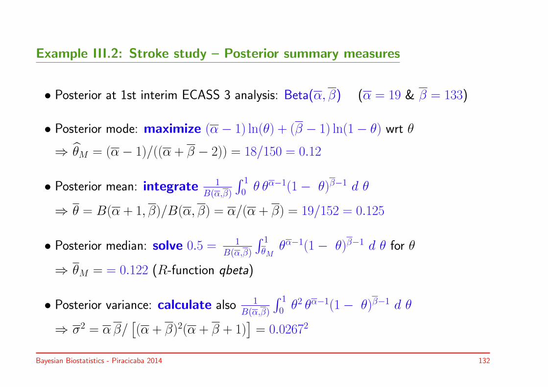
Example III.2: Stroke study – Posterior summary measures
• Posterior at 1st interim ECASS 3 analysis: Beta(α, β) (α = 19 & β = 133)
• Posterior mode: maximize (α− 1) ln(θ) + (β − 1) ln(1− θ) wrt θ
⇒ θM = (α− 1)/((α + β − 2)) = 18/150 = 0.12
• Posterior mean: integrate 1B(α,β)
∫ 1
0 θ θα−1(1− θ)β−1 d θ
⇒ θ = B(α + 1, β)/B(α, β) = α/(α + β) = 19/152 = 0.125
• Posterior median: solve 0.5 = 1B(α,β)
∫ 1
θMθα−1(1− θ)β−1 d θ for θ
⇒ θM = = 0.122 (R-function qbeta)
• Posterior variance: calculate also 1B(α,β)
∫ 1
0 θ2 θα−1(1− θ)β−1 d θ
⇒ σ2 = αβ/[(α + β)2(α + β + 1)
]= 0.02672
Bayesian Biostatistics - Piracicaba 2014 132
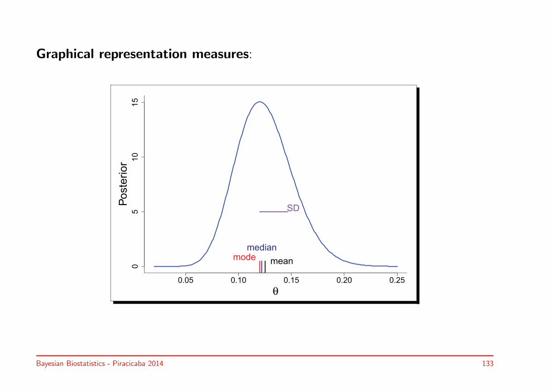
Graphical representation measures:
0.05 0.10 0.15 0.20 0.25
05
10
15
θ
Posterior
modemean
median
SD
Bayesian Biostatistics - Piracicaba 2014 133

Posterior summary measures:
• Posterior for µ (based on IBBENS prior):
Gaussian with µM ≡ µ ≡ µM
• Posterior mode=mean=median: µM = 327.2 mg/dl
• Posterior variance & SD: σ2 = 22.99 & σ = 4.79 mg/dl
Bayesian Biostatistics - Piracicaba 2014 134
3.3.2 Credible/credibility interval
• [a,b] = 95% credible interval (CI) for θ if P (a ≤ θ ≤ b |y) = 0.95
• Two types of 95% credible interval:
◃ 95% equal tail CI [a, b]:
AUC = 0.025 is left to a & AUC = 0.025 is right to b
◃ 95% highest posterior density (HPD) CI [a, b]:
[a, b] contains most plausible values of θ
• Properties:
◃ 100(1-α)% HPD CI = shortest interval with size (1− α) (Press, 2003)
◃ h(HPD CI) = HPD CI, but h(equal-tail CI) = equal-tail CI
◃ Symmetric posterior: equal tail = HPD CI
Bayesian Biostatistics - Piracicaba 2014 135
Example III.4: Dietary study – Interval estimation of dietary intake
• Posterior = N(µ, σ2)
• Obvious choice for a 95% CI is [µ− 1.96σ, µ + 1.96σ]
• Equal 95% tail CI = 95% HPD interval
• Results IBBENS-2 study:
◃ IBBENS prior distribution ⇒ 95% CI = [317.8, 336.6] mg/dl
◃ N(328; 10,000) prior ⇒ 95% CI = [285.6, 351.0] mg/dl
◃ Classical (frequentist) 95% confidence interval = [284.9, 351.1] mg/dl
Bayesian Biostatistics - Piracicaba 2014 136

Example III.5: Stroke study – Interval estimation of probability of SICH
• Posterior = Beta(19, 133)-distribution
• 95% equal tail CI (R function qbeta) = [0.077, 0.18] (see figure)
• 95% HPD interval = [0.075, 0.18] (see figure)
• Computations HPD interval: use R-function optimize
Bayesian Biostatistics - Piracicaba 2014 137
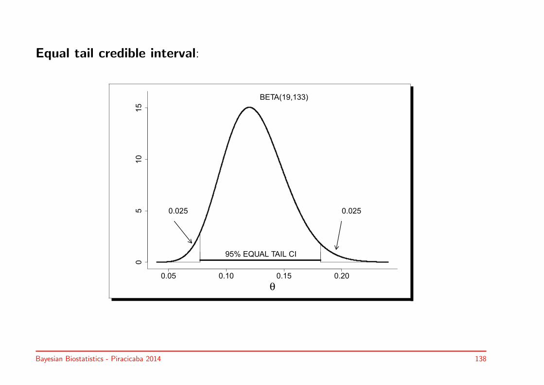
Equal tail credible interval:
0.05 0.10 0.15 0.20
05
10
15
θ
BETA(19,133)
95% EQUAL TAIL CI
0.025 0.025
Bayesian Biostatistics - Piracicaba 2014 138

HPD interval:
0.05 0.10 0.15 0.20
05
10
15
θ
Beta(19,133)(a)
95% HPD interval
−2.8 −2.4 −2.0 −1.6
0.0
0.5
1.0
1.5
2.0
ψ
(b)
log(95% original HPDI)
HPD interval is not-invariant to (monotone) transformations
Bayesian Biostatistics - Piracicaba 2014 139

3.4 Predictive distributions
Bayesian Biostatistics - Piracicaba 2014 140

3.4.1 Introduction
• Predictive distribution = distribution of a future observation y after havingobserved the sample {y1, . . . , yn}
• Two assumptions:
◃ Future observations are independent of current observations given θ
◃ Future observations have the same distribution (p(y | θ)) as the currentobservations
• We look at three cases: (a) binomial, (b) Gaussian and (c) Poisson
• We start with a binomial example
Bayesian Biostatistics - Piracicaba 2014 141
Example III.7: Stroke study – Predicting SICH incidence in interim analysis
• Before 1st interim analysis but given the pilot data:
Obtain an idea of the number of (future) rt-PA treated patients who will sufferfrom SICH in sample of size m = 50
• Distribution of y (given the pilot data)?
Bayesian Biostatistics - Piracicaba 2014 142
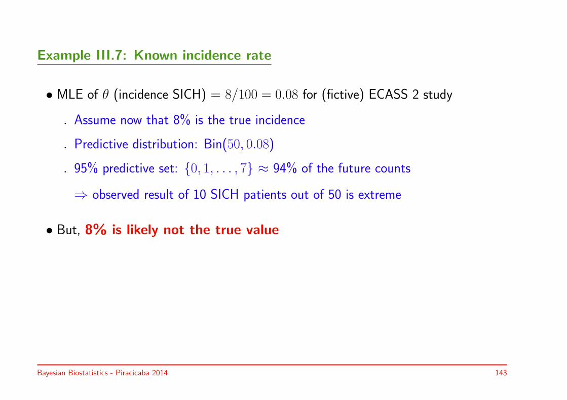
Example III.7: Known incidence rate
• MLE of θ (incidence SICH) = 8/100 = 0.08 for (fictive) ECASS 2 study
◃ Assume now that 8% is the true incidence
◃ Predictive distribution: Bin(50, 0.08)
◃ 95% predictive set: {0, 1, . . . , 7} ≈ 94% of the future counts
⇒ observed result of 10 SICH patients out of 50 is extreme
• But, 8% is likely not the true value
Bayesian Biostatistics - Piracicaba 2014 143

Binomial predictive distribution
0 2 4 6 8 10 12 14
0.0
00.0
50.1
00.1
50.2
0
# future RT−PA patients with SICH
Bin(50,0.08)
Ignores uncertainty in θ
Bayesian Biostatistics - Piracicaba 2014 144

Example III.7: Unknown incidence rate
• Uncertainty of θ expressed by posterior (ECASS 2 prior) = Beta(α, β)-distributionwith α = 9 and β = 93
• Distribution (likelihood) of m = 50 future SICH events is given by Bin(m, θ)
• Distribution of m = 50 future SICH events without knowing θ is weighted byposterior distribution = posterior predictive distribution (PPD)
• PPD = Beta-binomial distribution BB(m,α, β)
p(y|y) =
∫ 1
0
(m
y
)θy(1− θ)(m−y) θ
α−1(1− θ)β−1
B(α, β)dθ
=
(m
y
)B(y + α,m− y + β)
B(α, β)
Bayesian Biostatistics - Piracicaba 2014 145
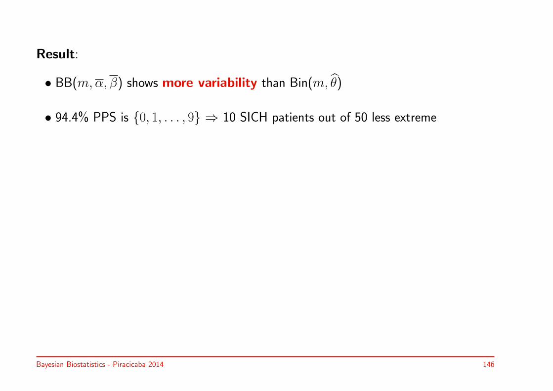
Result:
• BB(m,α, β) shows more variability than Bin(m, θ)
• 94.4% PPS is {0, 1, . . . , 9} ⇒ 10 SICH patients out of 50 less extreme
Bayesian Biostatistics - Piracicaba 2014 146
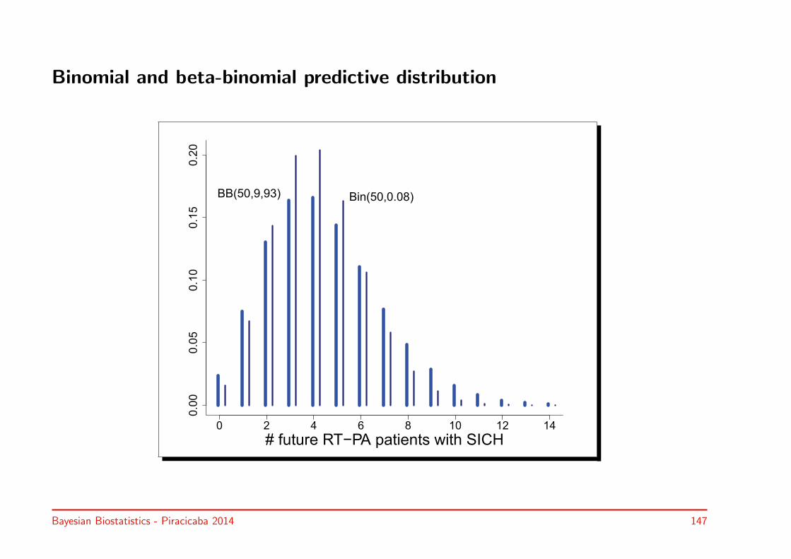
Binomial and beta-binomial predictive distribution
0 2 4 6 8 10 12 14
0.0
00.0
50.1
00.1
50.2
0
# future RT−PA patients with SICH
BB(50,9,93) Bin(50,0.08)
Bayesian Biostatistics - Piracicaba 2014 147

3.4.2 Posterior predictive distribution: General case
• Central idea: Take the posterior uncertainty into account
• Three cases:
◃ All mass (AUC ≈ 1) of p(θ | y) at θM ⇒ distribution of y: p(y | θM)
◃ All mass at θ1, . . . , θK ⇒ distribution of y:∑K
k=1 p(y | θk)p(θk | y)
◃ General case: posterior predictive distribution (PPD)
⇒ distribution of y
p(y | y) =∫p(y | θ)p(θ | y) dθ
• PPD expresses what we know about the distribution of the (future) ys
Bayesian Biostatistics - Piracicaba 2014 148

Example III.7: Second interim analysis
• Posterior after 1st interim analysis can be used:
◦ To compute PPD of the number SICH events in subsequent m treated rt-PApatients, to be evaluated in 2nd interim analysis
◦ As prior to be combined with the results in the 2nd interim analysis
◦ This is an example of the sequential use of Bayes theorem
Bayesian Biostatistics - Piracicaba 2014 149
Example III.6: SAP study – 95% normal range
• Serum alkaline phosphatase (alp) was measured on a prospective set of 250‘healthy’ patients by Topal et al (2003)
• Purpose: determine 95% normal range
• Recall: σ2 is known
Bayesian Biostatistics - Piracicaba 2014 150

Example III.6: Frequentist approach
• yi = 100/√alpi (i = 1, . . . , 250) ≈ normal distribution N(µ, σ2)
• µ = known
◃ 95% normal range for y: [µ− 1.96σ, µ+1.96σ], with µ = y = 7.11 (σ = 1.4)
⇒ 95% normal range for alp = [104.45, 508.95]
• µ = unknown
◃ 95% normal range for y: [y − 1.96σ√1 + 1/n, y + 1.96σ
√1 + 1/n]
⇒ 95% normal range for alp = [104.33, 510.18]
Bayesian Biostatistics - Piracicaba 2014 151

Histogram alp + 95% normal range
alp0 200 400 600 800 1000
0.0
00
0.0
01
0.0
02
0.0
03
0.0
04
0.0
05
0.0
06
95% REFERENCE RANGE
Bayesian Biostatistics - Piracicaba 2014 152
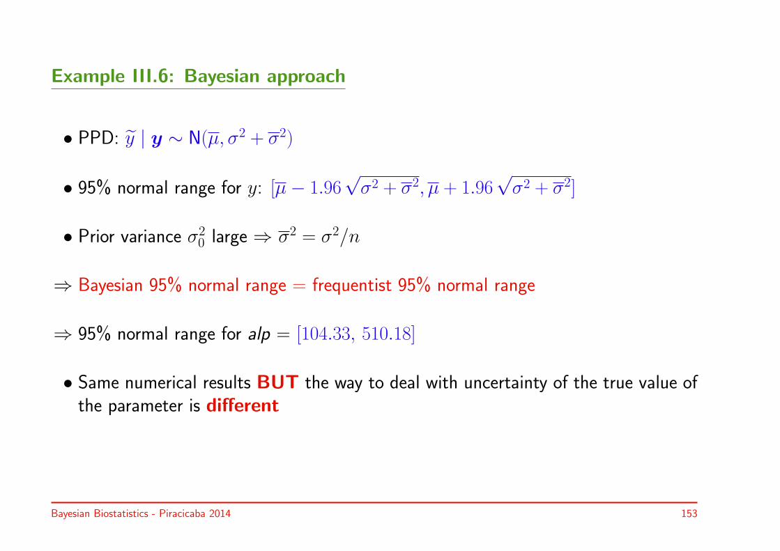
Example III.6: Bayesian approach
• PPD: y | y ∼ N(µ, σ2 + σ2)
• 95% normal range for y: [µ− 1.96√σ2 + σ2, µ + 1.96
√σ2 + σ2]
• Prior variance σ20 large ⇒ σ2 = σ2/n
⇒ Bayesian 95% normal range = frequentist 95% normal range
⇒ 95% normal range for alp = [104.33, 510.18]
• Same numerical results BUT the way to deal with uncertainty of the true value ofthe parameter is different
Bayesian Biostatistics - Piracicaba 2014 153

Example III.8: Caries study – PPD for caries experience
• Poisson likelihood + gamma prior ⇒ gamma posterior
• PPD = negative binomial distribution NB(α, β)
p(y|y) = Γ(α + y)
Γ(α) y!
(β
β + 1
)α (1
β + 1
)y
Bayesian Biostatistics - Piracicaba 2014 154
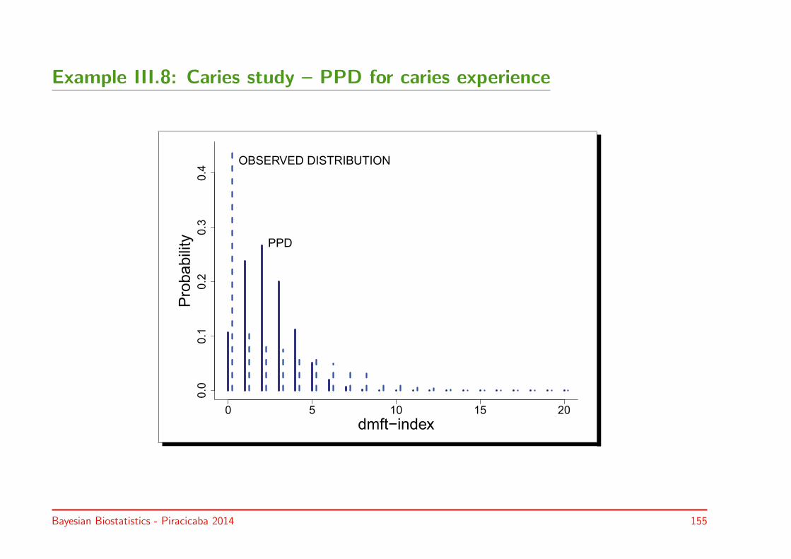
Example III.8: Caries study – PPD for caries experience
0 5 10 15 20
0.0
0.1
0.2
0.3
0.4
dmft−index
Pro
babili
ty
OBSERVED DISTRIBUTION
PPD
Bayesian Biostatistics - Piracicaba 2014 155

More applications of PPDs
See later:
• Determining when to stop a trial (see medical literature further)
• Given the past responses, predict the future responses of a patient
• Imputing missing data
• Model checking (Chapter 10)
Bayesian Biostatistics - Piracicaba 2014 156

3.5 Exchangeability
• Exchangeable:
◦ Order in {y1, y2, . . . , yn} is not important
◦ yi can be exchanged for yj without changing the problem/solution
◦ Extension of independence
• Exchangeability = key idea in (Bayesian) statistical inference
• Exchangeability of patients, trials, . . .
Bayesian Biostatistics - Piracicaba 2014 157

3.6 A normal approximation to the posterior
• When the sample is large and the statistical model is relatively simple (not manyparameters), then often the posterior looks like a normal distribution
• This property is typically used in the analysis of clinical trials
• In the book, we show that the normal approximation can work well for smallsample sizes (Example III.10)
• This is a nice property, but not crucial in Bayesian world, since all we need is theposterior
Bayesian Biostatistics - Piracicaba 2014 158

3.7 Numerical techniques to determine the posterior
• To compute the posterior, the product of likelihood with the prior needs to bedivided with the integral of that product
• In addition, to compute posterior mean, median, SD we also need to computeintegrals
• Here we see 2 possible ways to obtain in general the posterior and posteriorsummary measures:
◃ Numerical integration
◃ Sampling from the posterior
Bayesian Biostatistics - Piracicaba 2014 159

3.7.1 Numerical integration
Example III.11: Caries study – Posterior distribution for a lognormal prior
◦ Take first 10 children from STM study
◦ Assume dmft-index has Poisson(θ) with θ = mean dmft-index
◦ With prior: Gamma(3, 1) ⇒ Posterior: Gamma(29, 11)
◃ Replace gamma prior by lognormal prior, then posterior
∝ θ∑ni=1 yi−1e
−nθ−(log(θ)−µ0
2σ0
)2, (θ > 0)
◃ Posterior moments cannot be evaluated & AUC not known
◃ Mid-point approach provides AUC
Bayesian Biostatistics - Piracicaba 2014 160

Calculation AUC using mid-point approach:
1 2 3 4 5
0.0
00.0
20.0
40.0
60.0
80.1
0
θ
k x
PO
ST
ER
IOR
DE
NS
ITY
AUC =0.13
Bayesian Biostatistics - Piracicaba 2014 161

3.7.2 Sampling from the posterior distribution
• Monte Carlo integration: usefulness of sampling idea
• General purpose sampling algorithms
Bayesian Biostatistics - Piracicaba 2014 162
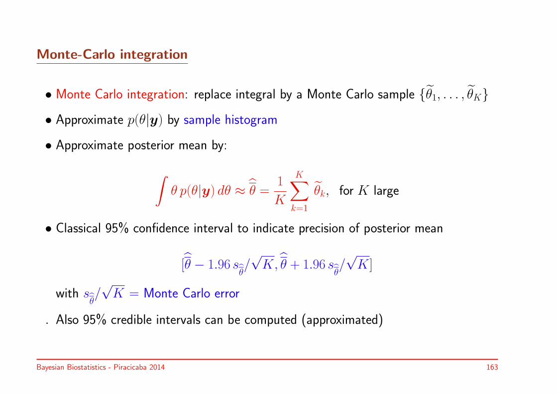
Monte-Carlo integration
• Monte Carlo integration: replace integral by a Monte Carlo sample {θ1, . . . , θK}
• Approximate p(θ|y) by sample histogram
• Approximate posterior mean by:
∫θ p(θ|y) dθ ≈ θ =
1
K
K∑k=1
θk, for K large
• Classical 95% confidence interval to indicate precision of posterior mean
[θ − 1.96 sθ/√K, θ + 1.96 s
θ/√K]
with sθ/√K = Monte Carlo error
◃ Also 95% credible intervals can be computed (approximated)
Bayesian Biostatistics - Piracicaba 2014 163
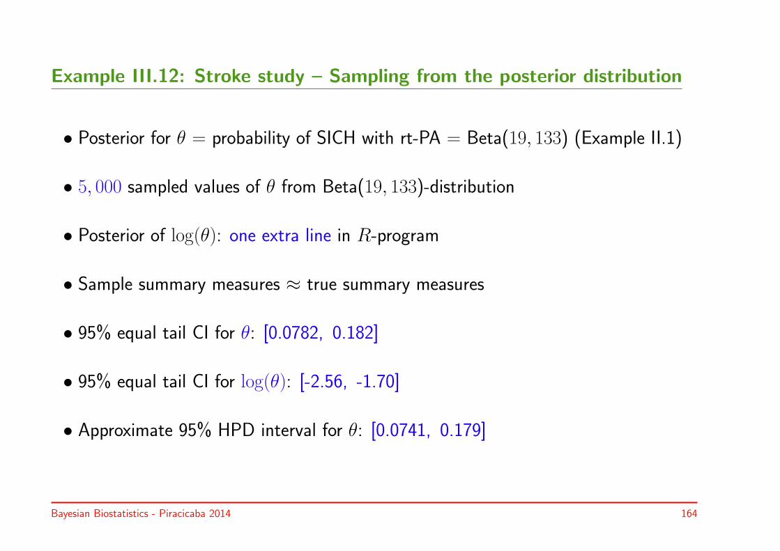
Example III.12: Stroke study – Sampling from the posterior distribution
• Posterior for θ = probability of SICH with rt-PA = Beta(19, 133) (Example II.1)
• 5, 000 sampled values of θ from Beta(19, 133)-distribution
• Posterior of log(θ): one extra line in R-program
• Sample summary measures ≈ true summary measures
• 95% equal tail CI for θ: [0.0782, 0.182]
• 95% equal tail CI for log(θ): [-2.56, -1.70]
• Approximate 95% HPD interval for θ: [0.0741, 0.179]
Bayesian Biostatistics - Piracicaba 2014 164
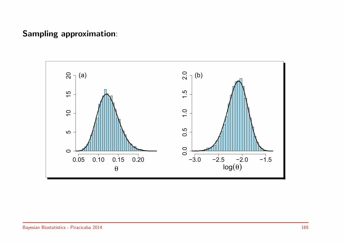
Sampling approximation:
θ
0.05 0.10 0.15 0.20
05
10
15
20 (a)
log(θ)−3.0 −2.5 −2.0 −1.5
0.0
0.5
1.0
1.5
2.0 (b)
Bayesian Biostatistics - Piracicaba 2014 165

Monte Carlo error (K=50)
�
���� ���� ����
��
��
��
��
black box = true posterior mean & red box = sampled posterior mean
Bayesian Biostatistics - Piracicaba 2014 166

General purpose sampling algorithms
• Many algorithms are available to sample from standard distributions
• Dedicated procedures/general purpose algorithms are needed for non-standarddistributions
• An important example: Accept-reject (AR) algorithm used by e.g. WinBUGS
◃ Generate samples from an instrumental distribution
◃ Then reject certain generated values to obtain sample from posterior
AR algorithm:only product of likelihood and prior is needed
Bayesian Biostatistics - Piracicaba 2014 167
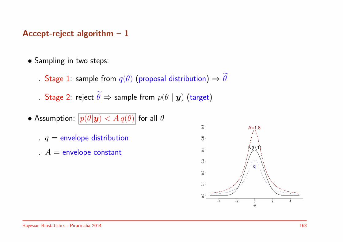
Accept-reject algorithm – 1
• Sampling in two steps:
◃ Stage 1: sample from q(θ) (proposal distribution) ⇒ θ
◃ Stage 2: reject θ ⇒ sample from p(θ | y) (target)
• Assumption: p(θ|y) < Aq(θ) for all θ
◃ q = envelope distribution
◃ A = envelope constant
−4 −2 0 2 40.0
0.1
0.2
0.3
0.4
0.5
0.6
θ
N(0,1)
q
A=1.8
Bayesian Biostatistics - Piracicaba 2014 168

Accept-reject algorithm – 2
• Stage 1: θ & u are drawn independently from q(θ) & U(0, 1)
• Stage 2:
◃ Accept: when u ≤ p(θ | y)/A q(θ)
◃ Reject: when u > p(θ | y)/A q(θ)
• Properties AR algorithm:
◃ Produces a sample from the posterior
◃ Only needs p(y | θ) p(θ)
◃ Probability of acceptance = 1/A
Bayesian Biostatistics - Piracicaba 2014 169
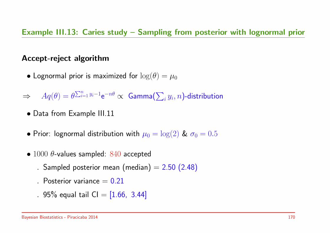
Example III.13: Caries study – Sampling from posterior with lognormal prior
Accept-reject algorithm
• Lognormal prior is maximized for log(θ) = µ0
⇒ Aq(θ) = θ∑ni=1 yi−1e−nθ ∝ Gamma(
∑i yi, n)-distribution
• Data from Example III.11
• Prior: lognormal distribution with µ0 = log(2) & σ0 = 0.5
• 1000 θ-values sampled: 840 accepted
◃ Sampled posterior mean (median) = 2.50 (2.48)
◃ Posterior variance = 0.21
◃ 95% equal tail CI = [1.66, 3.44]
Bayesian Biostatistics - Piracicaba 2014 170
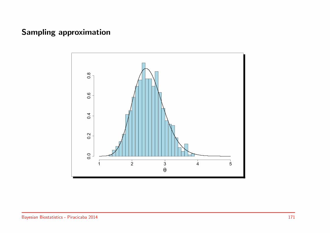
Sampling approximation
θ
1 2 3 4 5
0.0
0.2
0.4
0.6
0.8
Bayesian Biostatistics - Piracicaba 2014 171

Adaptive Rejection Sampling algorithms – 1
Adaptive Rejection Sampling (ARS) algorithm:
• Builds envelope function/density in an adaptive manner
• Builds squeezing function/density in an adaptive manner
• Envelope and squeezing density are log of piecewise linear functions with knots atsampled grid points
• Two special cases:
◃ Tangent method of ARS
◃ Derivative-free method of ARS
Bayesian Biostatistics - Piracicaba 2014 172
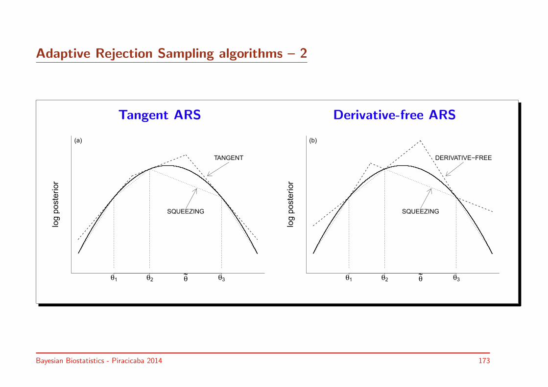
Adaptive Rejection Sampling algorithms – 2
Tangent ARS Derivative-free ARS
log p
oste
rior
θ1 θ2 θ~
θ3
TANGENT
SQUEEZING
(a)
log p
oste
rior
θ1 θ2 θ~
θ3
DERIVATIVE−FREE
SQUEEZING
(b)
Bayesian Biostatistics - Piracicaba 2014 173

Adaptive Rejection Sampling algorithms – 3
Properties ARS algorithms:
• Envelope function can be made arbitrarily close to target
• 5 to 10 grid points determine envelope density
• Squeezing density avoids (many) function evaluations
• Derivative-free ARS is implemented in WinBUGS
• ARMS algorithm: combination with Metropolis algorithm for non log-concavedistributions, implemented in Bayesian SAS procedures
Bayesian Biostatistics - Piracicaba 2014 174

3.7.3 Choice of posterior summary measures
• In practice: posterior summary measures are computed with sampling techniques
• Choice driven by available software:
◃ Mean, median and SD because provided by WinBUGS
◃ Mode almost never reported, but useful to compare with frequentist solution
◃ Equal tail CI (WinBUGS) & HPD (CODA and BOA)
Bayesian Biostatistics - Piracicaba 2014 175

3.8 Bayesian hypothesis testing
Two Bayesian tools for hypothesis testing H0: θ = θ0
• Based on credible interval:
◃ Direct use of credible interval:
◦ Is θ0 contained in 100(1-α)% CI? If not, then reject H0 in a Bayesian way!
◦ Popular when many parameters need to be evaluated, e.g. in regressionmodels
◃ Contour probability pB: P [p(θ | y) > p(θ0 | y)] ≡ (1− pB)
• Bayes factor: change of prior odds for H0 due to data (below)
Bayesian Biostatistics - Piracicaba 2014 176

Example III.14: Cross-over study – Use of CIs in Bayesian hypothesis testing
• 30 patients with systolic hypertension in cross-over study:
◦ Period 1: randomization to A or B
◦ Washout period
◦ Period 2: switch medication (A to B and B to A)
• θ = P(A better than B) & H0 : θ = θ0(= 0.5)
• Result: 21 patients better of with A than with B
• Testing:
◃ Frequentist: 2-sided binomial test (P = 0.043)
◃ Bayesian: U(0,1) prior + LBin(21 | 30, θ) = Beta(22, 10) posterior(pB = 0.023)
Bayesian Biostatistics - Piracicaba 2014 177
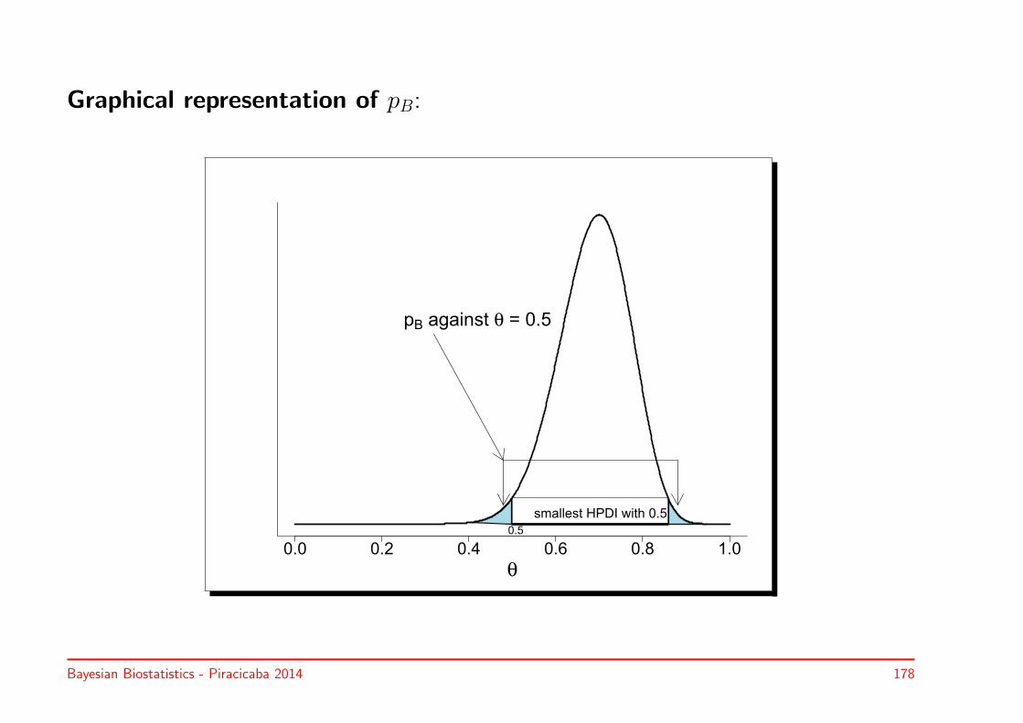
Graphical representation of pB:
0.0 0.2 0.4 0.6 0.8 1.0
θ
smallest HPDI with 0.5
pB against θ = 0.5
0.5
Bayesian Biostatistics - Piracicaba 2014 178

Predictive distribution of power and necessary sample size
• Classical power and sample size calculations make use of formulas to computepower for a given sample size, and necessary sample size for a chosen power
• However, there is often much uncertainty involved in the calculations because:
◦ Comparison of means: only a rough idea of the common SD is available to us,and there is no agreement on the aimed difference in efficacy
◦ Comparison of proportions: only a rough idea of the control rate is available tous, and there is no agreement on the aimed difference in efficacy
• Typically one tries a number of possible values of the required parameter valuesand inspects the variation in the calculation power/sample size
• Alternatively: use Bayesian approach with priors on parameters
• Here 2 examples: comparison of means & comparison of proportions
Bayesian Biostatistics - Piracicaba 2014 179
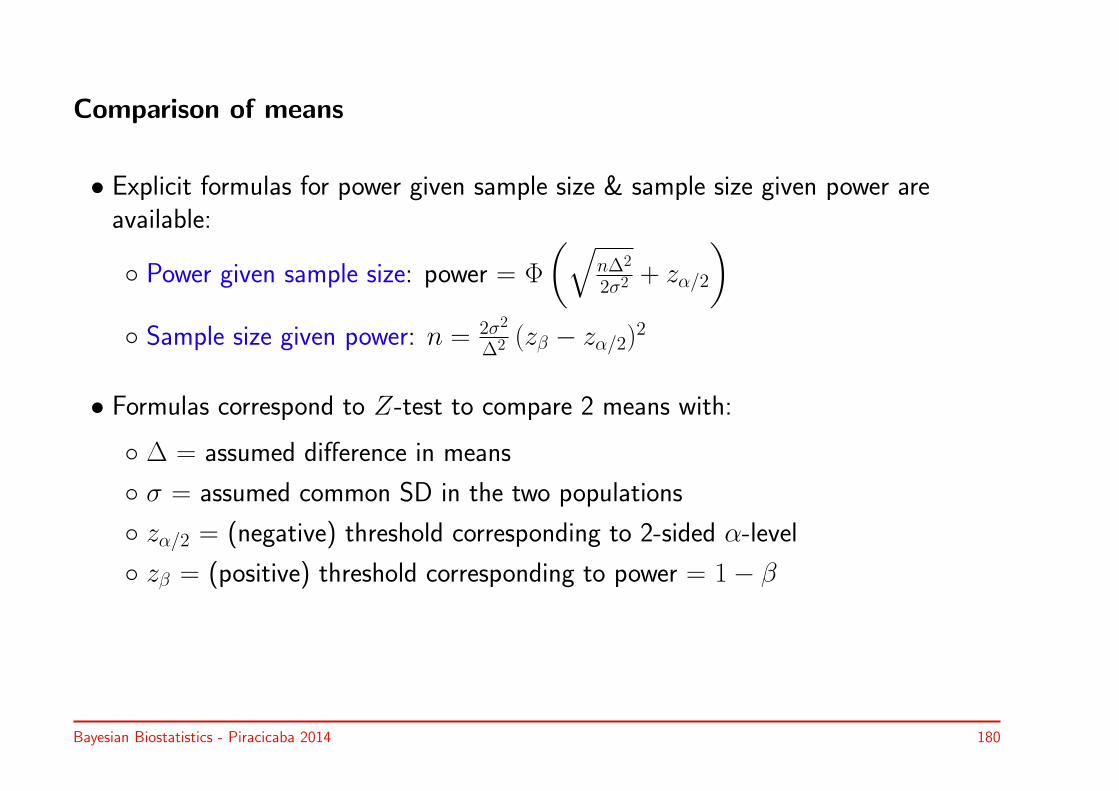
Comparison of means
• Explicit formulas for power given sample size & sample size given power areavailable:
◦ Power given sample size: power = Φ
(√n∆2
2σ2+ zα/2
)◦ Sample size given power: n = 2σ2
∆2 (zβ − zα/2)2
• Formulas correspond to Z-test to compare 2 means with:
◦ ∆ = assumed difference in means
◦ σ = assumed common SD in the two populations
◦ zα/2 = (negative) threshold corresponding to 2-sided α-level
◦ zβ = (positive) threshold corresponding to power = 1− β
Bayesian Biostatistics - Piracicaba 2014 180
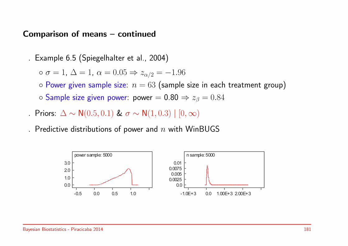
Comparison of means – continued
◃ Example 6.5 (Spiegelhalter et al., 2004)
◦ σ = 1, ∆ = 1, α = 0.05 ⇒ zα/2 = −1.96
◦ Power given sample size: n = 63 (sample size in each treatment group)
◦ Sample size given power: power = 0.80 ⇒ zβ = 0.84
◃ Priors: ∆ ∼ N(0.5, 0.1) & σ ∼ N(1, 0.3) | [0,∞)
◃ Predictive distributions of power and n with WinBUGS
power sample: 5000
-0.5 0.0 0.5 1.0
0.0
1.0
2.0
3.0
n sample: 5000
-1.0E+3 0.0 1.00E+3 2.00E+3
0.0
0.0025
0.005
0.0075
0.01
Bayesian Biostatistics - Piracicaba 2014 181
Pure Bayesian ways to determine necessary sample size
• The above approach is a combination of a Bayesian technique to take intoaccount the prior uncertainty of parameter values and the classical approach ofdetermining the sample size
• Alternative, Bayesian approaches for sample size calculation have been suggestedbased on the size of the posterior CI
• Note that the calculations require a design prior, i.e. a prior used to express theuncertainty of the parameters at the design stage. This design prior does not needto be the same as the prior used in the analysis
Bayesian Biostatistics - Piracicaba 2014 182

3.8.1 The Bayes factor
• Posterior probability for H0
p(H0 | y) =p(y | H0) p(H0)
p(y | H0) p(H0) + p(y | Ha) p(Ha)
• Bayes factor: BF (y)
p(H0 | y)1− p(H0 | y)
=p(y | H0)
p(y | Ha)× p(H0)
1− p(H0)
• Bayes factor =factor that transforms prior odds for H0 into posterior odds after observed the data
• Central in Bayesian inference, but not to all Bayesians
Bayesian Biostatistics - Piracicaba 2014 183
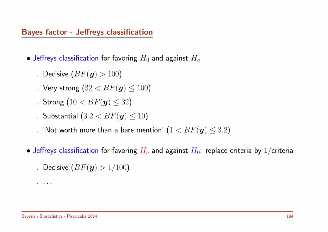
Bayes factor - Jeffreys classification
• Jeffreys classification for favoring H0 and against Ha
◃ Decisive (BF (y) > 100)
◃ Very strong (32 < BF (y) ≤ 100)
◃ Strong (10 < BF (y) ≤ 32)
◃ Substantial (3.2 < BF (y) ≤ 10)
◃ ‘Not worth more than a bare mention’ (1 < BF (y) ≤ 3.2)
• Jeffreys classification for favoring Ha and against H0: replace criteria by 1/criteria
◃ Decisive (BF (y) > 1/100)
◃ . . .
Bayesian Biostatistics - Piracicaba 2014 184

3.9 Medical literature on Bayesian methods in RCTs
Next three papers use above introduced summary measures + techniques
Bayesian Biostatistics - Piracicaba 2014 185

RCT example 1
47
Example 1: P.L. Shah et al. (Lancet, 378, 2011)
Based on
posterior
probabilities
Combined with
classical
statistical tests for
other endpoints
Bayesian Biostatistics - Piracicaba 2014 186

Bayesian Biostatistics - Piracicaba 2014 187
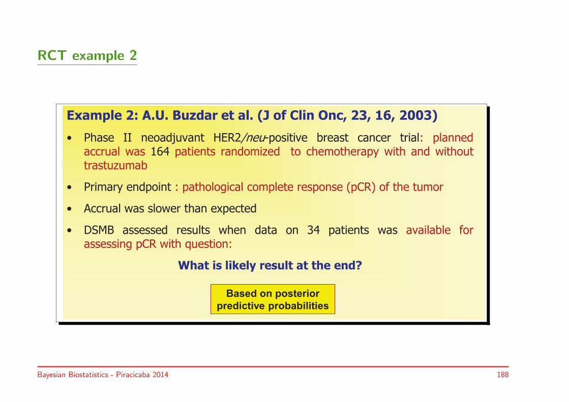
RCT example 2
Example 2: A.U. Buzdar et al. (J of Clin Onc, 23, 16, 2003)
• Phase II neoadjuvant HER2/neu-positive breast cancer trial: planned accrual was 164 patients randomized to chemotherapy with and without trastuzumab
• Primary endpoint : pathological complete response (pCR) of the tumor
• Accrual was slower than expected
• DSMB assessed results when data on 34 patients was available for assessing pCR with question:
What is likely result at the end?
Based on posterior
predictive probabilities
Bayesian Biostatistics - Piracicaba 2014 188
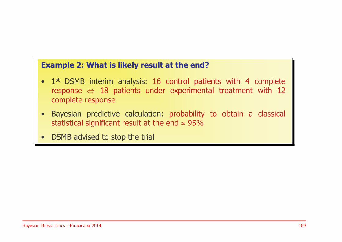
Example 2: What is likely result at the end?
• 1st DSMB interim analysis: 16 control patients with 4 complete response Û 18 patients under experimental treatment with 12 complete response
• Bayesian predictive calculation: probability to obtain a classical statistical significant result at the end » 95%
• DSMB advised to stop the trial
Bayesian Biostatistics - Piracicaba 2014 189
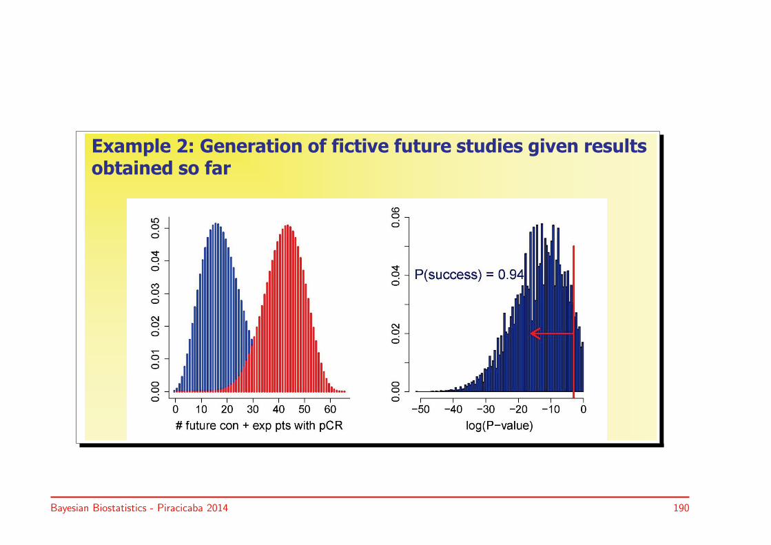
Example 2: Generation of fictive future studies given results obtained so far
Bayesian Biostatistics - Piracicaba 2014 190

RCT example 3
52
Example 3: Cannon et al. (Am Heart J, 2009, 158: 513-9.e3)
Bayesian Biostatistics - Piracicaba 2014 191

Example 3:
Bayesian Biostatistics - Piracicaba 2014 192
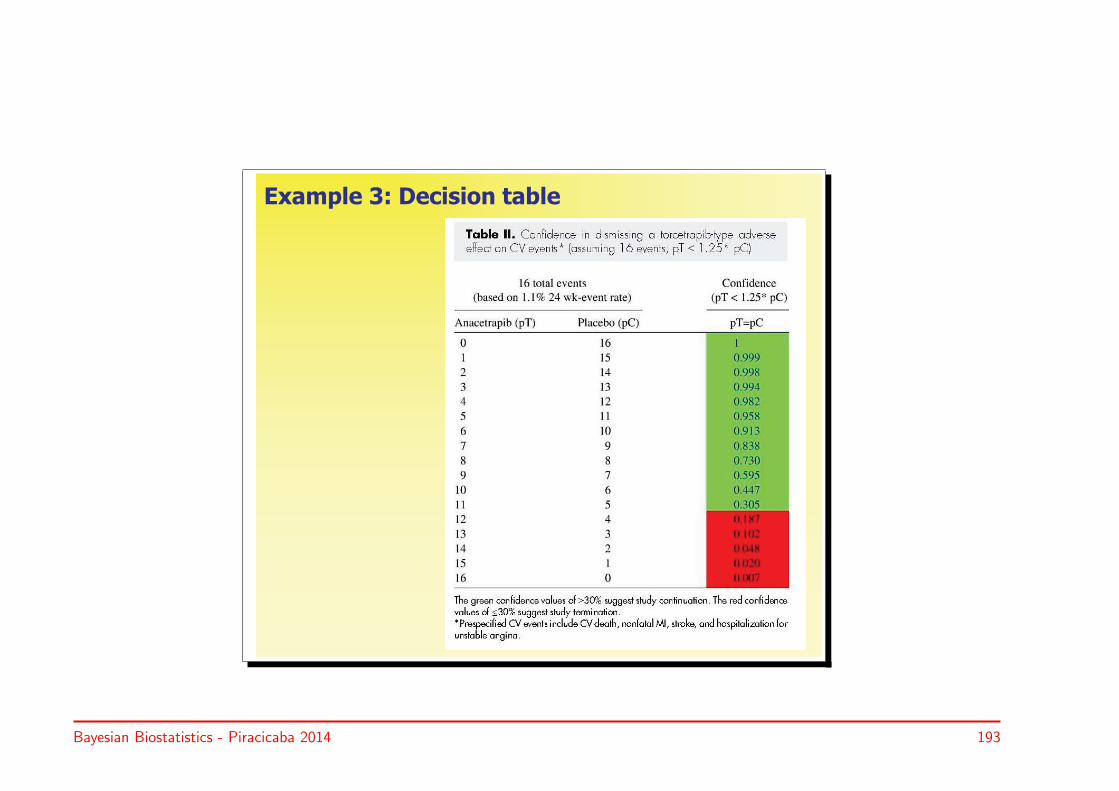
Example 3: Decision table
Bayesian Biostatistics - Piracicaba 2014 193

Take home messages
• Posterior distribution contains all information for statistical inference
• To characterize posterior, we can use:
◃ posterior mode, mean, median, variance, SD
◃ credible intervals: equal-tail, HPD
• Integration is key in Bayesian inference
• PPD = Bayesian tool to predict future
• No need to rely on large samples for Bayesian inference
Bayesian Biostatistics - Piracicaba 2014 194

• Bayesian hypothesis testing can be based on:
◃ credible intervals
◃ contour probability
◃ Bayes factor
• Sampling is a useful tool to replace integration
Bayesian Biostatistics - Piracicaba 2014 195