bayesian econometrics primer estimation of linearized dsge

Bayesian Econometrics Primer&

Estimation of linearized DSGE models

Stephane Adjemian

[email protected]

June, 2019

cba

http://creativecommons.org/licenses/by-sa/3.0/legalcode

https://mnemosyne.adjemian.eu/stepan-a/perfect-foresight-models

Introduction

I Full information Bayesian approach to linear(ized) DSGE models.

I Basically, this approach allows to incorporate prior knowledge aboutthe model and its parameters in the inference procedure.

I We first present the Bayesian approach in the case of a simple linearmodel for which closed form expressions are available.

I And we discuss issues specific to the estimation of DSGE models.

cba



Outline

Introduction

Maximum likelihood estimation

Prior and posterior beliefs

Point estimate

Marginal density of the sample

Forecasts

Likelihood of linear DSGE models

Simulation based posterior inference

Marginal density estimation

Posterior inference

cba



ML Estimation

I A model (M) defines a joint probability distribution parameterized(by θM) function over a sample of variables (say YT ):

f (YT |θM,M) (1)

I The parameters θM can be estimated by confronting the model tothe data through:

– Some moments of the DGP.– The probability density function of the DGP (all the moments).

I The first approach is a method of moments, the second one is alikelihood approach.

I Basically, a ML estimate for θM is obtained by maximizing thedensity of the sample with respect to the parameters (we seek thevalue of θM that maximizes the “probability of occurence” of thesample given by the Nature).

I In the sequel, we will denote L(θ) = f (YT |θ) the likelihood function,omitting the indexation with respect to the model when notnecessary.

cba



ML EstimationA simple static model

I As a first example, we consider the following model:

yt = µ0 + εt (2-a)

where εt ∼iidN (0, 1) and µ0 is an unknown finite real parameter.

I According to this model, yt is normally distributed:

yt |µ0 ∼ N (µ0, 1)

and E[ytys ] = 0 for all s 6= t.

I Suppose that a sample YT = y1, . . . , yT is available. Thelikelihood is defined by:

L(µ) = f (y1, . . . , yT |µ)

I Because the ys are iid, the joint conditional density is equal to aproduct of conditional densities:

L(µ) =T∏t=1

g(yt |µ)cba



ML EstimationA simple static model

I Since the model is linear and Gaussian:

L(µ) =T∏t=1

1√2π

e−(yt−µ)2

2

I Finally we have:

L(µ) = (2π)−T2 e−

12

∑Tt=1(yt−µ)2

(2-b)

I Note that the likelihood function depends on the data and theunknown parameter (otherwise we would have an identificationissue).

I Suppose that T = 1 (only one observation in the sample). We cangraphically determine the ML estimator of µ in this case.

cba



ML EstimationA simple static model (cont’d)

•

y1

f (y1|µ = µ)

YT

L(µ)

cba




•

•y1

f (y1|µ = µ)

YT

L(µ)

Clearly, the value of the density of y1 conditional on µ, ie the likelihood, is

maximized for µ = y1: for any µ 6= y1 we have f (y1|µ = µ) < f (y1|µ = y1)

cba




⇒ If we have only one observation, y1, the Maximum Likelihoodestimator is equal to the observation: µ = y1.

I This estimator is unbiased and its variance is 1.

I More generally, one can show that the maximum likelihoodestimator is equal to the sample mean:

µT =1

T

T∑t=1

yt (2-c)

I This estimator is unbiased and its variance is given by:

V [µT ] =1

T(2-d)

I Because V [µ] goes to zero as the sample size goes to infinity, weknow that this estimator converges in probability to the true valueµ0 of the unknown parameter:

µTproba−→

T→∞µ0

cba



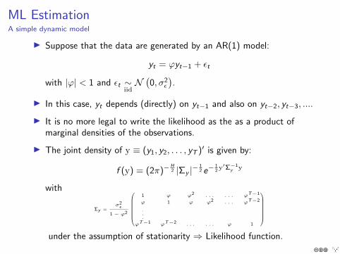
ML EstimationA simple dynamic model

I Suppose that the data are generated by an AR(1) model:

yt = ϕyt−1 + εt

with |ϕ| < 1 and εt ∼iidN(0, σ2

ε

).

I In this case, yt depends (directly) on yt−1 and also on yt−2, yt−3, ....

I It is no more legal to write the likelihood as the as a product ofmarginal densities of the observations.

I The joint density of y ≡ (y1, y2, . . . , yT )′ is given by:

f (y) = (2π)−H2 |Σy |−

12 e−

12 y′Σ−1

y y

with

Σy =σ2ε

1 − ϕ2

1 ϕ ϕ2 . . . . . . ϕT−1

ϕ 1 ϕ ϕ2 . . . ϕT−2

.

.

.

ϕT−1 ϕT−2 . . . . . . ϕ 1

under the assumption of stationarity ⇒ Likelihood function.

cba



Bayes theorem

I Let A and B be two events.

I Let P(A) and P(B) be the marginal probabilities.

I Let P(A ∩ B) be the joint probability of A and B.

I The Bayes theorem states that the probability of B conditional on Ais given by:

P(B|A) =P(A ∩ B)

P(A)

Splitting a joint probability

P(A ∩ B) = P(B|A)P(A) or P(A ∩ B) = P(A|B)P(B)

Conditioning inversion

⇒ P(B|A) =P(A|B)P(B)

P(A)

cba



ML EstimationA simple dynamic model (cont’d)

I The inverse of the covariance matrix, Σy , can be factorized asΣ−1

y = σ−2ε L′L with:

L =

√1 − ϕ2 0 0 . . . 0 0

−ϕ 1 0 . . . 0 00 −ϕ 1 . . . 0 0

.

.

.

.

.

.0 −ϕ 1

a T × T matrix.

I First manifestation of the Bayes theorem.

I The (ecact) likelihood function can be written equivalently as:

L(ϕ, σ2ε ) = (2π)−

T−12 σ−(T−1)

ε e− 1

2σ2ε

∑Tt=2(yt−ϕyt−1)2

×(2π)−12

(σ2ε

1− ϕ2

)− 12

e− 1−ϕ2

2σ2ε

y21

— Product of conditional densities, yt |yt−1 (the conditionallikelihood) and the marginal density of the initial condition y1.

— Marginal density of the initial condition, y1

cba



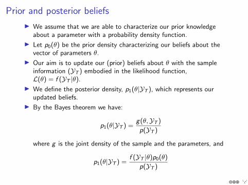
Prior and posterior beliefs

I We assume that we are able to characterize our prior knowledgeabout a parameter with a probability density function.

I Let p0(θ) be the prior density characterizing our beliefs about thevector of parameters θ.

I Our aim is to update our (prior) beliefs about θ with the sampleinformation (YT ) embodied in the likelihood function,L(θ) = f (YT |θ).

I We define the posterior density, p1(θ|YT ), which represents ourupdated beliefs.

I By the Bayes theorem we have:

p1(θ|YT ) =g(θ,YT )

p(YT )

where g is the joint density of the sample and the parameters, and

p1(θ|YT ) =f (YT |θ)p0(θ)

p(YT )

cba



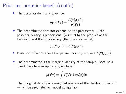
Prior and posterior beliefs (cont’d)

I The posterior density is given by:

p1(θ|YT ) =L(θ)p0(θ)

p(YT )

I The denominator does not depend on the parameters → theposterior density is proportional (w.r.t θ) to the product of thelikelihood and the prior density (the posterior kernel):

p1(θ|YT ) ∝ L(θ)p0(θ)

I Posterior inference about the parameters only requires L(θ)p0(θ).

I The denominator is the marginal density of the sample. Because adensity has to sum up to one, we have:

p(YT ) =

∫f (YT |θ)p0(θ)dθ

The marginal density is a weighted average of the likelihood function→ will be used later for model comparison.

cba



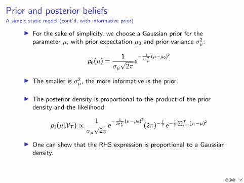
Prior and posterior beliefsA simple static model (cont’d, with informative prior)

I For the sake of simplicity, we choose a Gaussian prior for theparameter µ, with prior expectation µ0 and prior variance σ2

µ:

p0(µ) =1

σµ√

2πe− 1

2σ2µ

(µ−µ0)2

I The smaller is σ2µ, the more informative is the prior.

I The posterior density is proportional to the product of the priordensity and the likelihood:

p1(µ|YT ) ∝ 1

σµ√

2πe− 1

2σ2µ

(µ−µ0)2

(2π)−T2 e−

12

∑Tt=1(yt−µ)2

I One can show that the RHS expression is proportional to a Gaussiandensity.

cba




I The likelihood can be equivalently written as:

L(µ) = (2π)−T2 e−

12 (νs2+T (µ−µ)2)

with ν = T − 1 and

s2 =1

ν

T∑t=1

(yt − µ)2

I s2 and µ are sufficient statistics: they convey all the necessarysample information regarding the inference w.r.t µ.

I The likelihood is proportional to a Gaussian density centered on µwith variance 1/T .

I The posterior density:

p1(µ|YT ) ∝ 1

σµ(√

2π)T+1

e− 1

2σ2µ

(µ−µ0)2− ν2 s2− T

2 (µ−µ)2

cba




I Previous expression can be simplified by omitting all themultiplicative terms not related to µ (this is legal because we areinterested in a proportionality w.r.t µ):

p1(µ|YT ) ∝ e− 1

2σ2µ

(µ−µ0)2− T2 (µ−µ)2

I We develop the quadratic forms and remove all the terms appearingadditively (under the exponential function); we obtain:

p1(µ|YT ) ∝ e− 1

2 (σ−2µ +T)

(µ−

T µ+µ0σ−2µ

T+σ−2µ

)2

I We recognize the expression of a Gaussian density (up to a scaleparameter that does not depend on µ).

cba



Let A(µ) = 1σ2µ

(µ − µ0

)2 + T (µ − µ)2. We establish the last expression of the posterior kernel by rewriting A(µ) as:

A(µ) = T (µ − µ)2 +1

σ2µ

(µ − µ0)2

= T(µ

2 + µ2 − 2µµ)

+1

σ2µ

(µ

2 + µ20 − 2µµ0

)

=

T +1

σ2µ

µ2 − 2µ

T µ +1

σ2µ

µ0

+

T µ2 +1

σ2µ

µ20

=

T +1

σ2µ

µ2 − 2µ

T µ + 1σ2µµ0

T + 1σ2µ

+

T µ2 +1

σ2µ

µ20

=

T +1

σ2µ

µ −

T µ + 1σ2µµ0

T + 1σ2µ

2

+

T µ2 +1

σ2µ

µ20

−

(T µ + 1

σ2µµ0

)2

T + 1σ2µ

In the last equality, the two last additive terms do not depend on µ and can be therefore omitted.

cba




I The posterior distribution is Gaussian with (posterior) expectation:

E [µ] =T µ+ 1

σ2µµ0

T + 1σ2µ

and (posterior) variance:

V [µ] =1

T + 1σ2µ

I As soon as the amount of prior information is positive (σ2µ <∞) the

posterior variance is less than the variance of the maximumlikelihood estimator (1/T).

I The posterior expectation is a convex combination of the maximumlikelihood estimator and the prior expectation.

cba




I The Bayesian approach can be interpreted as a bridge between thecalibration approach (σ2

µ = 0, infinite amount of prior information)

and the ML approach (σ2µ =∞, no prior information):

E [µ] −−−−→σ2µ→0

µ0

andE [µ] −−−−→

σ2µ→∞

µ

I The more important is the amount of information in the sample, thesmaller will be the gap between the posterior expectation and theML estimator.

cba



Prior and posterior beliefsA simple dynamic model (cont’d, flat prior)

I For a real parameter, the prior is proportional to 1.

p0(ϕ) ∝ 1

I For a positive parameter, the prior of the log of the prior isproportional to 1.

p0(log σ2ε ) ∝ 1 ⇔ p0(σ2

ε ) ∝ 1

σε

Flat prior for AR(1) model

p0

(ϕ, σ2

ε

)∝ 1

σε

→ Parameters ϕ and σ2ε are a priori independent.

→ This prior is not a pdf!

cba



Prior and posterior beliefsA simple dynamic model (cont’d, flat prior)

I Use the conditional likelihood (omitting the marginal density of thefirst observation).

I The posterior density is:

p1(ϕ, σ2ε ) ∝ σ−1

ε︸︷︷︸Prior

(2π)−T−1

2 σ−(T−1)ε e

− 12σ2ε

∑Tt=2(yt−ϕyt−1)2︸︷︷︸

Conditional likelihood

∝ σ−Tε e− 1

2σ2ε

∑Tt=2(yt−ϕyt−1)2

Posterior density

ϕ|σ2ε ,YT ∼ N

(∑Tt=2 ytyt−1∑Tt=2 y

2t−1

,σ2ε∑T

t=2 y2t−1

)

σ2ε |YT ∼ IG

(T − 2,

T∑t=2

ε2t

)cba



Point estimate

I The outcome of the Bayesian approach is a (posterior) probabilitydensity function.

I But people generally expect much less information: a point estimateis often enough for most practical purposes (a single value for eachparameter with a measure of uncertainty).

⇒ We need to reduce a distribution to a “representative” point.

I Let L(θ, θ) be the loss incurred if we choose θ while θ is the truevalue.

I The idea is to choose the value of θ that minimizes this loss... Butthe true value of θ is obviously unknown, so we minimize the(posterior) expected loss instead:

θ? = arg minθ

E[L(θ, θ)

]= arg min

θ

∫L(θ, θ)p1(θ|YT )dθ

I The choice of the loss function is purely arbitrary, for each loss wewill obtain a different point estimate.

cba



Point estimateQuadratic loss function (L2 norm)

I Suppose that the loss function is quadratic:

L(θ, θ) = (θ − θ)′Ω(θ − θ)

where Ω is a symmetric positive definite matrix. Note that thisfunction returns a (real) scalar.

I The (posterior) expectation of the loss is:

E[L(θ, θ)

]= E

[(θ − θ)′Ω(θ − θ)

]= E

[(θ − Eθ −

(θ − Eθ

))′Ω(θ − Eθ −

(θ − Eθ

))]= E

[(θ − Eθ)′ Ω (θ − Eθ)

]+ (θ − Eθ)′Ω(θ − Eθ)

I Noting that the first term does not depend on the choice variable, θ,the expected loss is trivially minimized when θ is equal to the(posterior) expectation of θ:

θ? = E [θ]

⇒ If the loss is quadratic the optimal point estimate is the posteriorexpectation.

cba



Point estimateGeneralized bsolute value loss function (quantiles)

I Suppose that the (univariate) loss function is:

L(θ, θ) =

α(θ − θ) if θ ≥ θβ(θ − θ) if θ < θ

with β 6= α two positive parameters.

I The (posterior) expectation of the loss is:

E[L(θ, θ)

]= β

∫ θ

−∞(θ − θ)p1(θ|YT )dθ + α

∫ ∞θ

(θ − θ)p1(θ|YT )dθ

I F.O.C.

β

∫ θ?

−∞p1(θ|YT )dθ − α

∫ ∞θ?

p1(θ|YT )dθ = 0

⇒ (β + α)

∫ θ?

−∞p1(θ|YT )dθ = α

∫ ∞−∞

p1(θ|YT )dθ

⇔∫ θ?


α

α + β(→ any posterior quantile)

cba



Marginal density of the sample

I If we are only interested in inference about the parameters, themarginal density of the data, p(YT ), can be omitted.

I We already saw that the marginal density of the data is:

p(YT ) =

∫f (YT |θ)p0(θ)dθ

I The marginal density of the sample acts as a constant of integrationin the expression of the posterior density.

I The marginal density of the sample is an average of the likelihoodfunction (for different values of the estimated parameters) weightedby the prior density.

⇒ The marginal density of the sample is a measure of fit, which doesnot depend on the parameters (because we integrate them out).

I Note that, theoretically, it is possible to compute the marginaldensity of the sample (conditional on a model) without estimatingthe parameters.

cba



Marginal density of the sampleA simple static model (cont’d)

I Suppose again that the sample size is T = 1. The likelihood is givenby:

f (YT |µ) =1√2π

e−12 (y1−µ)2

I The marginal density is then given by:

p(YT ) =

∫ ∞−∞

f (y1|µ)p0(µ)dµ

= (2πσµ)−1

∫ ∞−∞

e− 1

2

((y1−µ)2+

(µ−µ0)2

σ2µ

)dµ

=1√

2π(1 + σ2µ)

e− (y1−µ0)2

2(1+σ2µ)

I We can directly obtain the same result by noting that y1 is the sumof two Gaussian random variables: N (0, 1) and N

(µ0, σ

2µ

).

cba



Marginal density of the sampleModel comparison

I Suppose we have two models A and B (with two associated vectorsof deep parameters θA and θB) estimated using the same sampleYT .

I For each model I = A,B we can evaluate, at least theoretically, themarginal density of the data conditional on the model:

p(YT |I) =

∫f (YT |θI , I)p0(θI |I)dθI

by integrating out the deep parameters θI from the posterior kernel.

I p(YT |I) measures the fit of model I. If we have to choose betweenmodels A and B we will select the model with the highest marginaldensity of the sample.

I Note that models A and B need not to be nested (for instance, wedo not require that θA be a subset of θB) for the comparison tomake sense, because the compared marginal densities do not dependon the parameters. The classical approach (comparisons oflikelihoods) by requiring nested models is much less obvious.

cba



Marginal density of the sampleModel comparison (cont’d)

I Suppose we have a prior distribution over models A and B: p(A)and p(B).

I Again, using the Bayes theorem we can compute the posteriordistribution over models:

p(I|YT ) =p(I)p(YT |I)∑

I=A,B p(I)p(YT |I)

I This formula may easily be generalized to a collection of N models.

I In the literature posterior odds ratio, defined as:

p(A|YT )

p(B|YT )=

p(A)

p(B)

p(YT |A)

p(YT |B)

are often used to discriminate between different models. If theposterior odds ratio is large (>100) we can safely choose model A.

cba



Marginal density of the sampleModel comparison (cont’d)

I Note that we do not necessarily have to choose one model.

I Even if a model has a smaller posterior probability (or marginaldensity) it may provide useful informations in some directions (orfrequencies), so we should not discard this information.

I An alternative is to mix the models.

I If these models are used for forecasting inflation, we can report anaverage of the forecasts weighted by the posterior probabilities,p(I|YT ), instead of the forecasts of the best model (in terms ofmarginal density) → Bayesian averaging.

cba



Predictive density

I We often seek to use the estimated model to do inference aboutunobserved variables.

I The most obvious example is the forecasting exercise.I In the Bayesian context the density of an unobserved variable (for

instance the future growth of GDP) given the sample, is called apredictive density.

I Let y be a vector of unobserved variables. The joint posteriordensity of y and θ is:

p1(y , θ|YT ) = g(y |θ,YT )p1(θ|YT )

I The posterior predictive density is obtained by integrating out theparameters:

p(y |YT ) =

∫g(y |θ,YT )p1(θ|YT )dθ

The posterior predictive density is the average of the density of yknowing the parameters weighted by the posterior density of theparameters.

cba



Predictive densityA simple static model (cont’d)

I Suppose that we want to do inference about the out of samplevariable yT+1 (forecast).

I The density of yT+1 conditional on the sample and on the parameteris:

g(yT+1|µ,YT ) ∝ e−12 (yT+1−µ)2

Note that this conditional density does not depend on YT becausethe model is static (for an autoregressive model, at least yT wouldappear under the quadratic term).

I Remember that the posterior density of µ is:

p1(µ|YT ) ∝ e−1

2V[µ] (µ−E[µ])2

where E[µ] and V[µ] are the posterior first and second ordermoments obtained earlier.

cba




I The predictive density for yT+1 is given by:

p(yT+1|YT ) =

∫g(yT+1|µ,YT )p1(µ|YT )dµ

∝∫ ∞−∞

e−12 (yT+1−µ)2− 1

2V[µ] (µ−E[µ])2

dµ

I The terms under the exponential in the last expression can berewritten as:[

1 +1

V[µ]

](µ− yT+1 + V[µ]−1

1 + V[µ]−1

)2

+V[µ]−1

1 + V[µ]−1(yT+1 − E[µ])2

cba




I By substitution in the expression of the predictive density for yT+1

we obtain:

p(yT+1|YT ) ∝∫ ∞−∞

e− 1

2 [1+ 1V[µ] ]

(µ− yT+1+V[µ]−1

1+V[µ]−1

)2

− 12

V[µ]−1

1+V[µ]−1 (yT+1−E[µ])2

dµ

∝ e− 1

2V[µ]−1

1+V[µ]−1 (yT+1−E[µ])2∫ ∞−∞

e− 1

2 [1+ 1V[µ] ]

(µ− yT+1+V[µ]−1

1+V[µ]−1

)2

dµ

∝ e−12

11+V[µ] (yT+1−E[µ])2

I Unsurprisingly, we recognize the Gaussian density:

yT+1|YT ∼ N (E[µ], 1 + V[µ])

I We would have obtained directly the same result by first noting thatyT+1 is the sum of two Gaussian random variables: N (E[µ],V[µ])(for the estimated parameter) and N (0, 1) (for the error term).

cba



Predictive densityPoint prediction

I For reporting our forecast, we may want to select one point in thepredictive distribution.

I We proceed as for the point estimate by choosing an arbitrary lossfunction and minimizing the posterior expected loss.

I Usually the expectation of the predictive distribution is reported(rationalized with a quadratic loss function).

cba



Estimation of DSGE modelsStructural form

I We suppose that the DSGE model can be cast in the following form:

Et [Fθ(yt+1, yt , yt−1, εt)] = 0 (2)

with εt ∼ iid (0,Σε) is a random vector (r × 1) of structuralinnovations, yt ∈ Λ ⊆ Rn a vector of endogenous variables,Fθ : Λ3 × Rr → Λ a real function in C2 parameterized by a realvector θ ∈ Θ ⊆ Rq gathering the deep parameters of the model.

I The model is stochastic, forward looking and non linear.

I We want to estimate (a subset of) θ. For any estimation approach(indirect inference, simulated moments, maximum likelihood,...) weneed first to solve this model.

cba



Estimation of DSGE modelsReduced form

I In the sequel we consider a local linear approximation around thedeterministic steady state of the non linear model.

I The solution of the linearized model (the reduced form) is:

yt = y(θ) + A(θ) (yt−1 − y(θ)) + B(θ)εt

where the steady state, y(θ), and matrices A(θ) and B(θ) arenonlinear functions of the deep parameters.

I The unconditional covariance matrix of y solves:

Σy = A(θ)ΣyA(θ)′ + B(θ)ΣεB(θ)′

and the autocovariance function is defined as:

Γh = A(θ)Γh−1 ∀h ≥ 1

with Γ0 = Σy and Γ−h = Γ′h.

cba



Estimation of DSGE modelsLikelihood

I Let YT = y?1 , y?2 , . . . , y

?T be the sample, with

y?t = Zyt

where Z is a p × n selection matrix.

I The likelihood is the density of the sample. If the structuralinnovations are Gaussian:

L = (2π)−pT2 |Σy? |−

12 e−

12 (y?−y?)′Σ−1

y?(y?−y?)

with y? = (y?1′ , y?2

′ , . . . , y?T′)′ a Tp × 1 vector, and

Σy? =

Γ?0 Γ?1 Γ?2 . . . . . . . . . Γ?T−1

Γ?1′ Γ?0 Γ?1 Γ?2 . . . . . . Γ?T−2

Γ?2′ Γ?1

′ Γ?0 Γ?1 . . . . . . Γ?T−3...

Γ?T−1′ Γ?T−2

′ . . . . . . . . . Γ?1′ Γ?0

where Γ?h = ZΓhZ

′. → Symmetric block Toeplitz matrix.

cba



Estimation of DSGE modelsKalman filter

I The well known Kalman filter bayesian recursive algorithm can beused to evaluate the likelihood:

vt = y?t − y(θ)? − Zyt

Ft = ZPtZ′+V [η]

Kt = A(θ)PtA(θ)′F−1t

yt+1 = A(θ)yt + Ktvt

Pt+1 = A(θ)Pt(A(θ)− KtZ )′ + B(θ)ΣεB(θ)′

for t = 1, . . . ,T , with initial condition y0 = y?0 − y? and P0 given bythe ergodic distribution of y?.

I The (log)-likelihood is:

lnL = −Tp

2ln(2π)− 1

2

T∑t=1

|Ft | −1

2v ′tF−1t vt

I Ft is full rank only if we have at least as many innovations asobserved variables.

cba



Estimation of DSGE modelsPosterior distribution

I We know that the posterior density is proportional to the likelihoodtimes the prior density.

I Because we do not have closed form expressions for the reducedform of the model and the likelihood, we cannot obtain analyticalresults about the posterior density.

I Posterior inference can be done by considering:

1. Asymptotic (Gaussian) approximation of the posterior density.2. Simulation based methods (exact up to the randomness inherent to

these methods).

cba



Simulation based posterior inference

I We need a simulation approach if we want to obtain exact results (ienot relying on asymptotic approximation).

I Noting that:

E [ϕ(ψ)] =

∫Ψ

ϕ(ψ)p1(ψ|YT )dψ

we can use the empirical mean of(ϕ(ψ(1)), ϕ(ψ(2)), . . . , ϕ(ψ(n))

),

where ψ(i) are draws from the posterior distribution to evaluate theexpectation of ϕ(ψ). The approxomation error goes to zero whenn→∞.

I We need to simulate draws from the posterior distribution.

⇒ Metropolis-Hastings algorithm.

cba



Simulation based posterior inferenceA simple example – a –

I Imagine we want to obtain some draws from a N (0, 4) distribution...

I But we are only able to draw from N (0, 1) and we don’t realize thatwe should simply multiply by 2 the draws from a standard normaldistribution.

I The idea is to build a stochastic process whose limiting distributionis N (0, 4).

I We define the following AR(1) process:

xt = ρxt−1 + εt

with εt ∼ N (0, 1), |ρ| < 1 and x0 = 0.

I We just have to choose ρ such that the asymptotic distribution ofxt is N (0, 4).

cba



Simulation based posterior inferenceA simple example – b –

We have:

I x1 = ε1 ∼ N (0, 1)

I x2 = ρε1 + ε2 ∼ N(0, 1 + ρ2

)I x3 = ρ2ε1 + ρε2 + ε3 ∼ N

(0, 1 + ρ2 + ρ4

)I ...

I xT = ρT−1ε1 + ρT−2ε2 + · · ·+ εT ∼ N(0, 1 + ρ2 + . . . ρ2(T−1)

)I ...

I And asymptotically

x∞ ∼ N(

0,1

1− ρ2

)So that V∞[xt ] = 4 iff ρ = ±

√3

2 .

cba



Simulation based posterior inferenceA simple example – c –

I If we simulate enough draws from this Gaussian autoregressivestochastic process, we can replicate the targeted distribution.

I In this case it is very simple because we know exactly the targeteddistribution and we are able to obtain some draws from itsstandardized version.

I This is far from true with dsge models. For instance, we even don’thave an analytical expression for the posterior density.

cba



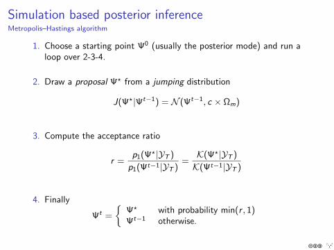
Simulation based posterior inferenceMetropolis–Hastings algorithm

1. Choose a starting point Ψ0 (usually the posterior mode) and run aloop over 2-3-4.

2. Draw a proposal Ψ? from a jumping distribution

J(Ψ?|Ψt−1) = N (Ψt−1, c × Ωm)

3. Compute the acceptance ratio

r =p1(Ψ?|YT )

p1(Ψt−1|YT )=K(Ψ?|YT )

K(Ψt−1|YT )

4. Finally

Ψt =

Ψ? with probability min(r , 1)Ψt−1 otherwise.

cba



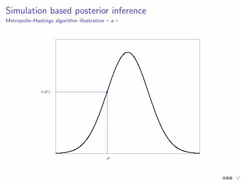
Simulation based posterior inferenceMetropolis–Hastings algorithm illustration – a –

θo

K (θo)

cba



Simulation based posterior inferenceMetropolis–Hastings algorithm illustration – b –

θo

K (θo)

θ1 = θ∗

K(θ1)

cba



Simulation based posterior inferenceMetropolis–Hastings algorithm illustration – c –

θo

K (θo)

θ1

K(θ1)

θ∗

K(θ∗) ??

cba



Simulation based posterior inferenceTuning of the Metropolis–Hastings algorithm

I How should we choose the scale factor c (variance of the jumpingdistribution)?

I We define the acceptance ratio as the number of accepted drawsover the number of proposals:

R =# accepted draws

# proposals

I We do not want to have R close to 0 because it means that wereject almost all the proposals.

I We neither want to have R close to 1 because it means that weaccept almost all the proposals and that most likely the jumpingdistribution proposes too small jumps.

I In the literature, authors generally target an acceptance ratio aroundone third, although there is no rational for that choice in the case ofDSGE models.

I The scale factor, c , must be adjusted to match this target:I If R is too low, c should be reduced (why?).I If R is too high, c should be increased (why?).

cba



Simulation based posterior inferenceConvergence of the Metropolis–Hastings algorithm

I Another issue is the number of draws required to obtain an accurateestimation of the posterior distribution.

I We need to asses the convergence of the Metropolis Hastingsalgorithm.

I The estimated posterior distribution should be:

(i) stable when we increase the number of simulations.(ii) independent of the initial condition.

I To check that the estimated posterior distribution satisfy these twoproperties, we can run multiple Monte Carlo Markov Chains andverify that:

(i) Moments are constant if the number of simulations is increased.(ii) Pooled and Within moments are identical.

I This approach is implemented in Dynare (see the manual).

cba



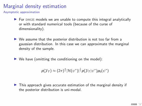
Marginal density estimationAsymptotic approximation

I For dsge models we are unable to compute this integral analyticallyor with standard numerical tools (because of the curse ofdimensionality).

I We assume that the posterior distribution is not too far from agaussian distribution. In this case we can approximate the marginaldensity of the sample.

I We have (omitting the conditioning on the model):

p(YT ) ≈ (2π)n2 |H(ψ∗)| 12 p(YT |ψ∗)p0(ψ∗)

I This approach gives accurate estimation of the marginal density ifthe posterior distribution is uni-modal.

cba



Marginal density estimationA first simulation based method

I We can estimate the marginal density using a Monte-Carlo approach

p(YT ) =1

B

B∑b=1

p(YT |ψ(b))

where ψ(b) is sampled from the prior distribution.

I p(YT ) −→B→∞

p(YT ).

I But this method is highly inefficient, because:I p(YT ) may have a huge variance (even infinite in some pathological

cases).I We are not using simulations already done to obtain the posterior

distribution (ie Metropolis-Hastings draws).

cba



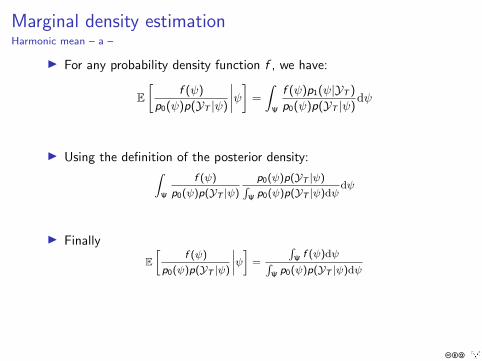
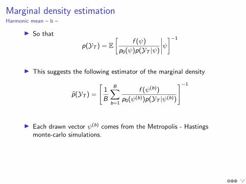
Marginal density estimationHarmonic mean – b –

I So that

p(YT ) = E[

f (ψ)

p0(ψ)p(YT |ψ)

∣∣∣∣ψ]−1

I This suggests the following estimator of the marginal density

p(YT ) =

[1

B

B∑b=1

f (ψ(b))

p0(ψ(b))p(YT |ψ(b))

]−1

I Each drawn vector ψ(b) comes from the Metropolis - Hastingsmonte-carlo simulations.

cba



Marginal density estimationHarmonic mean – c –

I The preceding proof holds if we replace f (θ) by 1# Simple Harmonic Mean estimator. But this estimator may alsohave a huge variance.

I The density f (θ) may be interpreted as a weighting function, wewant to give less importance to extremal values of θ.

I Geweke (1999) suggests to use a truncated gaussian function(modified harmonic mean estimator).

cba



Marginal density estimationHarmonic mean – d –

ψ =1

B

B∑b=1

ψ(b)

Ω =1

B

B∑b=1

(ψ(b) − ψ)′(ψ(b) − ψ)

I For some p ∈ (0, 1) we define

Ψ =ψ : (ψ(b) − ψ)′Ω

−1(ψ(b) − ψ) ≤ χ2

1−p(n)

I ... And take

f (ψ) = p−1(2π)−n2 |Ω|−

12 e−

12

(ψ−ψ)′Ω−1(ψ−ψ)I

Ψ(ψ)

cba



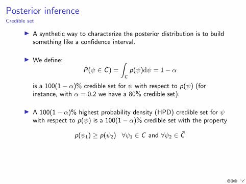
Posterior inferenceCredible set

I A synthetic way to characterize the posterior distribution is to buildsomething like a confidence interval.

I We define:

P(ψ ∈ C ) =

∫C

p(ψ)dψ = 1− α

is a 100(1− α)% credible set for ψ with respect to p(ψ) (forinstance, with α = 0.2 we have a 80% credible set).

I A 100(1− α)% highest probability density (HPD) credible set for ψwith respect to p(ψ) is a 100(1− α)% credible set with the property

p(ψ1) ≥ p(ψ2) ∀ψ1 ∈ C and ∀ψ2 ∈ C

cba



Posterior inferenceDensity

I To obtain a view of the posterior distribution we can estimate themarginal posterior densities (for each parameter of the model).

I We use a non parametric estimator:

f (ψ) =1

Nh

N∑i=1

K

(ψ − ψ(i)

h

)where N is the number of draws in the metropolis, ψ is a point

where we want to evaluate the posterior density, ψ(i) is a draw fromthe metropolis, K (•) is a kernel (gaussian by default in Dynare) andh is a bandwidth parameter.

I In Dynare the bandwidth parameter is, by default, optimally chosenconsidering the Silverman’s rule of thumb (controling for therepetitions in the MCMC draws).

cba



Posterior inferencePredictive density

I Knowing the posterior distribution of the model’s parameters, wecan forecast the endogenous variables of the model.

I We define the posterior predictive density as follows:

p(Y|YT ) =

∫Ψ

p(Y, ψ|YT )dψ

where, for instance, Y might be yT+1. Knowing thatp(Y, ψ|YT ) = p(Y|ψ,YT )p1(ψ|YT ) we have:

p(Y|YT ) =

∫Ψ

p(Y|ψ,YT )p1(ψ|YT )dψ

cba



Posterior inferencePredictive density

I In practice, we just have to

1. sample vectors of parameters from the posterior distribution (usingthe MCMC draws),

2. compute the forecast (also IRFs if needed) for each vector ofparameters.

I In the end of this process we obtain an empirical posteriordistribution for the forecasts (IRFs).

I If our loss function is quadratic, we can then report a point forecastby computing the mean of this empirical posterior distribution.

cba



Posterior inferenceIntegration

I More generally, the MCMC draws can be used to estimate anymoments of the parameters (or function of the parameters).

I We have

E [h(ψ)] =

∫Ψ

h(ψ)p(ψ|YT )dψ

≈ 1

N

N∑i=1

h(ψ(i))

where ψ(i) is a metropolis draw and h is any continuous function.

cba



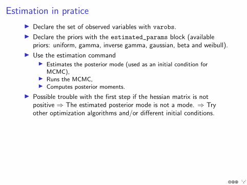
Estimation in pratice

I Declare the set of observed variables with varobs.

I Declare the priors with the estimated_params block (availablepriors: uniform, gamma, inverse gamma, gaussian, beta and weibull).

I Use the estimation commandI Estimates the posterior mode (used as an initial condition for

MCMC),I Runs the MCMC,I Computes posterior moments.

I Possible trouble with the first step if the hessian matrix is notpositive ⇒ The estimated posterior mode is not a mode. ⇒ Tryother optimization algorithms and/or different initial conditions.

cba



bayesian econometrics primer estimation of linearized dsge

Documents