bayesian estimation with dynare · pdf fileintroduction likelihood posterior mcmc estimating...
TRANSCRIPT
Introduction Likelihood Posterior MCMC Estimating in Dynare
Bayesian Estimation with Dynare
Colin Caines
UBC
March 4, 2016

Introduction Likelihood Posterior MCMC Estimating in Dynare
Overview
• Can we use information in model solution to estimate parameters?
• Does the data tell us about more than just the mode?
• Can we compute P(q |X ), the distribution of parameters q given data?

Introduction Likelihood Posterior MCMC Estimating in Dynare
Bayes Law for Posterior
• Given P(q) and data X
P(q |X ) =P(X |q) ·P(q)R
P(X |q 0)P(q 0)dq 0
- P(q |X ) is posterior distribution- P(q) is prior distribution, this is a choice- P(X |q) is likelihood function, comes from model solution-
RP(X |q 0)P(q 0)dq 0 is normalization constant
=) P(q |X ) µ L(X |q) ·P(q)
Introduction Likelihood Posterior MCMC Estimating in Dynare
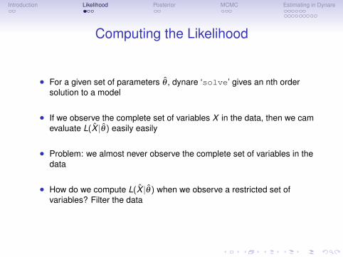
Computing the Likelihood
• For a given set of parameters q , dynare ‘solve’ gives an nth ordersolution to a model
• If we observe the complete set of variables X in the data, then we camevaluate L(X |q) easily easily
• Problem: we almost never observe the complete set of variables in thedata
• How do we compute L(X |q) when we observe a restricted set ofvariables? Filter the data
Introduction Likelihood Posterior MCMC Estimating in Dynare
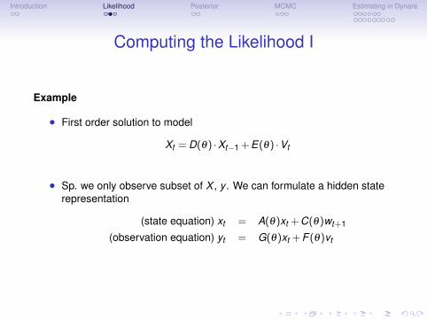
Computing the Likelihood I
Example
• First order solution to model
X
t
= D(q) ·Xt�1 +E(q) ·V
t
• Sp. we only observe subset of X , y . We can formulate a hidden staterepresentation
(state equation) x
t
= A(q)xt
+C(q)wt+1
(observation equation) y
t
= G(q)xt
+F (q)vt
Introduction Likelihood Posterior MCMC Estimating in Dynare
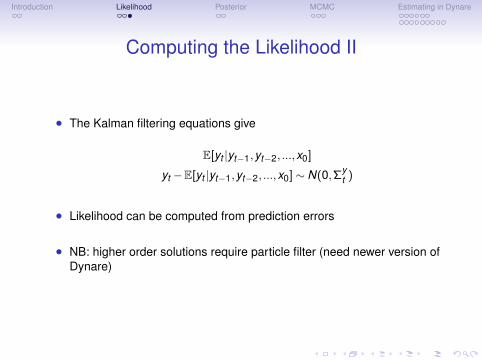
Computing the Likelihood II
• The Kalman filtering equations give
E[yt
|yt�1,yt�2, ...,x0]
y
t
�E[yt
|yt�1,yt�2, ...,x0]⇠ N(0,⌃y
t
)
• Likelihood can be computed from prediction errors
• NB: higher order solutions require particle filter (need newer version ofDynare)
Introduction Likelihood Posterior MCMC Estimating in Dynare
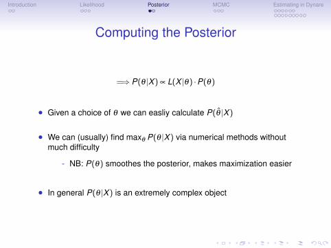
Computing the Posterior
=) P(q |X ) µ L(X |q) ·P(q)
• Given a choice of q we can easliy calculate P(q |X )
• We can (usually) find maxq P(q |X ) via numerical methods withoutmuch difficulty
- NB: P(q) smoothes the posterior, makes maximization easier
• In general P(q |X ) is an extremely complex object
Introduction Likelihood Posterior MCMC Estimating in Dynare
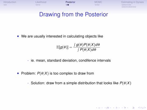
Drawing from the Posterior
• We are usually interested in calculating objects like
E[g(q)] =R
g(q)P(q |X )dqRP(q |X )dq
- ie. mean, standard deviation, condifence intervals
• Problem: P(q |X ) is too complex to draw from
- Solution: draw from a simple distribution that looks like P(q |X )
Introduction Likelihood Posterior MCMC Estimating in Dynare
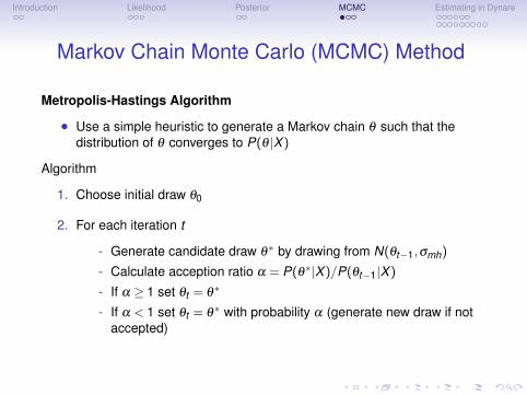
Markov Chain Monte Carlo (MCMC) Method
Metropolis-Hastings Algorithm
• Use a simple heuristic to generate a Markov chain q such that thedistribution of q converges to P(q |X )
Algorithm
1. Choose initial draw q0
2. For each iteration t
- Generate candidate draw q⇤ by drawing from N(qt�1,s
mh
)
- Calculate acception ratio a = P(q⇤|X )/P(qt�1|X )
- If a � 1 set qt
= q⇤
- If a < 1 set qt
= q⇤ with probability a (generate new draw if notaccepted)
Introduction Likelihood Posterior MCMC Estimating in Dynare
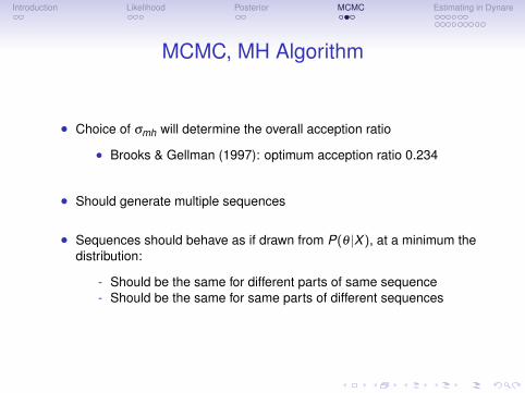
MCMC, MH Algorithm
• Choice of smh
will determine the overall acception ratio
• Brooks & Gellman (1997): optimum acception ratio 0.234
• Should generate multiple sequences
• Sequences should behave as if drawn from P(q |X ), at a minimum thedistribution:
- Should be the same for different parts of same sequence- Should be the same for same parts of different sequences
Introduction Likelihood Posterior MCMC Estimating in Dynare
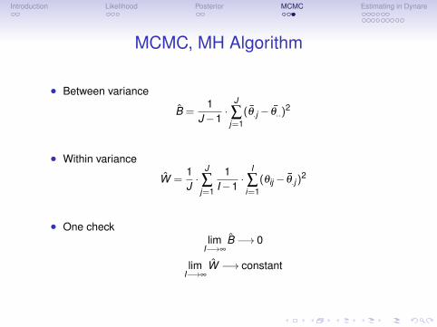
MCMC, MH Algorithm
• Between variance
B =1
J �1·
J
Âj=1
(q.j � q..)2
• Within variance
W =1J
·J
Âj=1
1I �1
·I
Âi=1
(qij
� q.j )2
• One checklim
I�!•B �! 0
limI�!•
W �! constant
Introduction Likelihood Posterior MCMC Estimating in Dynare
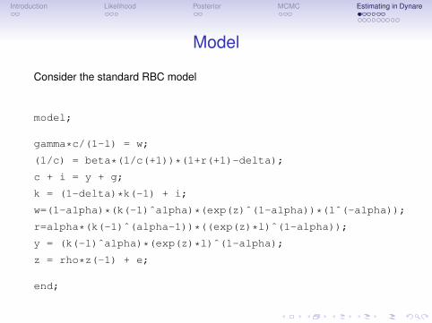
Model
Consider the standard RBC model
model;
gamma*c/(1-l) = w;
(1/c) = beta*(1/c(+1))*(1+r(+1)-delta);
c + i = y + g;
k = (1-delta)*k(-1) + i;
w=(1-alpha)*(k(-1)ˆalpha)*(exp(z)ˆ(1-alpha))*(lˆ(-alpha));
r=alpha*(k(-1)ˆ(alpha-1))*((exp(z)*l)ˆ(1-alpha));
y = (k(-1)ˆalpha)*(exp(z)*l)ˆ(1-alpha);
z = rho*z(-1) + e;
end;
Introduction Likelihood Posterior MCMC Estimating in Dynare
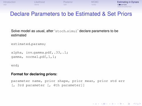
Declare Parameters to be Estimated & Set Priors
Solve model as usual, after ‘stoch simul’ declare parameters to beestimated
estimated params;
alpha, inv gamma pdf,.33,.1;gamma, normal pdf,1,1;
end;
Format for declaring priors:
parameter name, prior shape, prior mean, prior std err[, 3rd parameter [, 4th parameter]]
Introduction Likelihood Posterior MCMC Estimating in Dynare
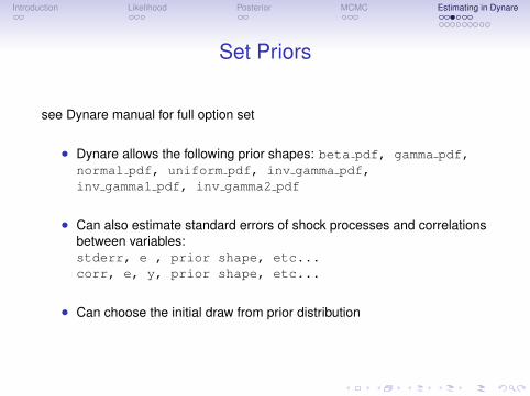
Set Priors
see Dynare manual for full option set
• Dynare allows the following prior shapes: beta pdf, gamma pdf,normal pdf, uniform pdf, inv gamma pdf,inv gamma1 pdf, inv gamma2 pdf
• Can also estimate standard errors of shock processes and correlationsbetween variables:stderr, e , prior shape, etc...corr, e, y, prior shape, etc...
• Can choose the initial draw from prior distribution
Introduction Likelihood Posterior MCMC Estimating in Dynare
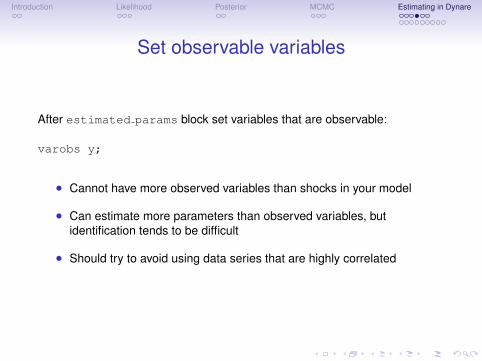
Set observable variables
After estimated params block set variables that are observable:
varobs y;
• Cannot have more observed variables than shocks in your model
• Can estimate more parameters than observed variables, butidentification tends to be difficult
• Should try to avoid using data series that are highly correlated

Introduction Likelihood Posterior MCMC Estimating in Dynare
Estimation
Estimation command:
estimation(datafile=z ycildata,mh nblocks=5,mh replic=10000,mh jscale=.5);
You must have data file in the search path
• Dynare can read .m, .mat, or .xls files• File must have variable names at the begining of columns, names must
match variable names in mod file• Dynare can filter data before estimation (‘prefilter=1’)
Introduction Likelihood Posterior MCMC Estimating in Dynare
Estimation
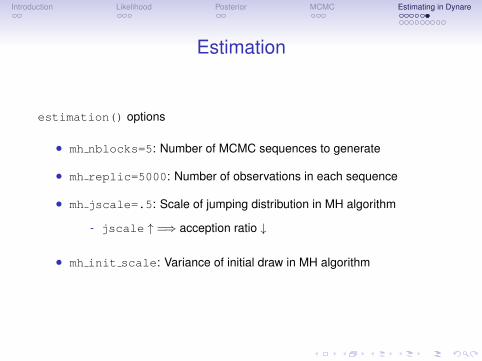
estimation() options
• mh nblocks=5: Number of MCMC sequences to generate
• mh replic=5000: Number of observations in each sequence
• mh jscale=.5: Scale of jumping distribution in MH algorithm
- jscale " =) acception ratio #
• mh init scale: Variance of initial draw in MH algorithm
Introduction Likelihood Posterior MCMC Estimating in Dynare
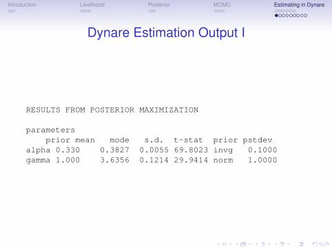
Dynare Estimation Output I
RESULTS FROM POSTERIOR MAXIMIZATION
parametersprior mean mode s.d. t-stat prior pstdev
alpha 0.330 0.3827 0.0055 69.8023 invg 0.1000gamma 1.000 3.6356 0.1214 29.9414 norm 1.0000
Introduction Likelihood Posterior MCMC Estimating in Dynare
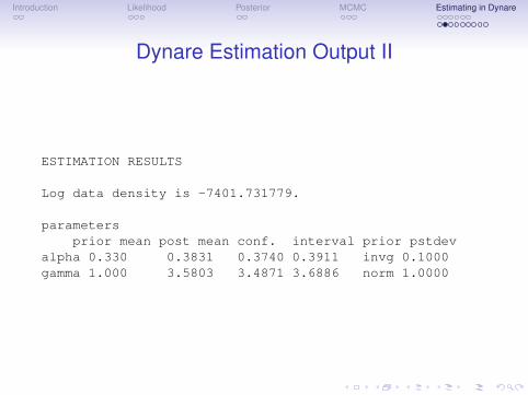
Dynare Estimation Output II
ESTIMATION RESULTS
Log data density is -7401.731779.
parametersprior mean post mean conf. interval prior pstdev
alpha 0.330 0.3831 0.3740 0.3911 invg 0.1000gamma 1.000 3.5803 3.4871 3.6886 norm 1.0000
Introduction Likelihood Posterior MCMC Estimating in Dynare
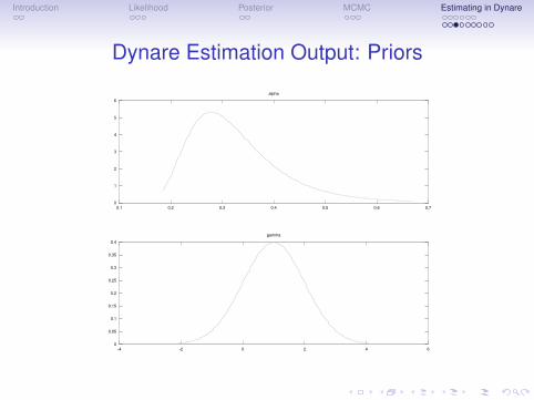
Dynare Estimation Output: Priors
0
0.05
0.1
0.15
0.2
0.25
0.3
0.35
0.4
-4 -2 0 2 4 6
gamma
0
1
2
3
4
5
6
0.1 0.2 0.3 0.4 0.5 0.6 0.7
alpha

Introduction Likelihood Posterior MCMC Estimating in Dynare
Dynare Estimation Output: Posterior
• Want to see some evidence that your estimater posterior is not beingdriven by your choice of prior
Introduction Likelihood Posterior MCMC Estimating in Dynare
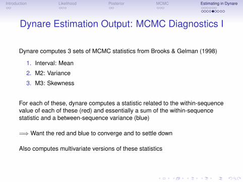
Dynare Estimation Output: MCMC Diagnostics I
Dynare computes 3 sets of MCMC statistics from Brooks & Gelman (1998)
1. Interval: Mean
2. M2: Variance
3. M3: Skewness
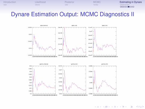
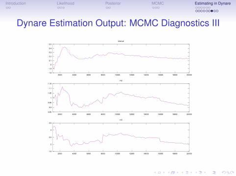
For each of these, dynare computes a statistic related to the within-sequencevalue of each of these (red) and essentially a sum of the within-sequencestatistic and a between-sequence variance (blue)
=) Want the red and blue to converge and to settle down
Also computes multivariate versions of these statistics
Introduction Likelihood Posterior MCMC Estimating in Dynare
Dynare Estimation Output: MCMC Diagnostics II
0.0026
0.0028
0.003
0.0032
0.0034
0.0036
2000400060008000100001200014000160001800020000
gamma (m3)
0.014
0.0145
0.015
0.0155
0.016
0.0165
0.017
0.0175
2000400060008000100001200014000160001800020000
gamma (m2)
0.3
0.305
0.31
0.315
0.32
0.325
0.33
0.335
0.34
0.345
0.35
2000400060008000100001200014000160001800020000
gamma (Interval)
2.4e-07
2.5e-07
2.6e-07
2.7e-07
2.8e-07
2.9e-07
3e-07
3.1e-07
2000400060008000100001200014000160001800020000
alpha (m3)
2.9e-05
3e-05
3.1e-05
3.2e-05
3.3e-05
3.4e-05
2000400060008000100001200014000160001800020000
alpha (m2)
0.0135
0.014
0.0145
0.015
0.0155
2000400060008000100001200014000160001800020000
alpha (Interval)
Introduction Likelihood Posterior MCMC Estimating in Dynare
Dynare Estimation Output: MCMC Diagnostics III
1.5
2
2.5
3
3.5
2000 4000 6000 8000 10000 12000 14000 16000 18000 20000
m3
0.85
0.9
0.95
1
1.05
1.1
1.15
2000 4000 6000 8000 10000 12000 14000 16000 18000 20000
m2
1.8
1.9
2
2.1
2.2
2.3
2.4
2.5
2000 4000 6000 8000 10000 12000 14000 16000 18000 20000
Interval
Introduction Likelihood Posterior MCMC Estimating in Dynare
Bayesian IRF
estimation(...,bayesian irf) varlist
• will compute the Bayesian IRFS of all variables in varlist
• results stored in structure oo .PosteriorIRF.dsge
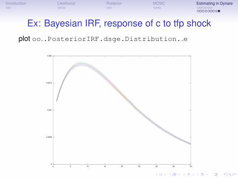
Introduction Likelihood Posterior MCMC Estimating in Dynare
Ex: Bayesian IRF, response of c to tfp shockplot oo .PosteriorIRF.dsge.Distribution. e
0
0.0005
0.001
0.0015
0.002
0 5 10 15 20 25 30 35 40