bayesian methods in the selection of farm animals for breeding
TRANSCRIPT
1vs a a fl ArYt *
tJN
Bayesian Methods
in the Selection of Farm Animals
for Breeding
Mehmet Ziya Firat
Ph. D.
University of Edinburgh
1995

Abstract
The purpose of this thesis is to implement Bayesian methods to solve theoretical and
practical statistical problems inthe selection of animals for breeding. The thesis is there-
fore focused mainly on the calculation of posterior distributions of variance components
and functions of them, and the construction of optimum Bayesian selection methods for
a single quantitative trait and multiple traits. Half-sib family structures are considered
throughout, although the theory considered is more general in its application.
Conventional and Bayesian methods for variance components estimation are re-
viewed from an animal breeding point of view, with emphasis on balanced data, but
unbalanced data are also discussed.
In Bayesian statistics the necessary integrations in several dimensions are usually
difficult to perform by analytical means. A Gibbs sampling approach, which yields
output readily translated into required inference summaries, is applied to integrations
using suitable families of prior distributions. Gibbs sampling output is then used to
develop appropriate graphical methods for summarizing posterior distributions of genetic
and phenotypic parameters, and to calculate the posterior expectations of breeding
values and the expected progress using different selection procedures.
The selection of farm animals for breeding is treated as a decision problem in which
the utility of choosing a given number of individuals is assumed to be proportional to
the sum of the corresponding breeding values. The Bayesian selection procedure in this
case is contrasted with conventional procedures based on point estimates of parameters,
including a method based on modified parameter estimates known as bonding. Point
estimates can be poor and frequently nonsensical even when breeding data on hundreds
of animals are used. It is shown that Bayesian procedures give improved selection deci-
sions as they make use of all the information on parameters rather than just providing
point estimates.
Finally, the restricted maximum likelihood method (REML) and the Gibbs sampling
procedure are appliedto single trait and multiple-trait sire models for test day milkyields
obtained on 23,873 British Holstein-Friesian heifers in 7,973 herds, these being progeny
of 40 proven and 649 young sires. Inferences and selection procedures based on REML
estimates and posterior expectations are compared.

Acknowledgements
First and foremost, I would like to express my sincere thanks to my supervisor
Dr C.M. Theobald at the Department of Mathematics and Statistics for his gen-
erous help, patience and supervision throughout the period of research leading to
this thesis. My thanks are also due to my second supervisor Dr Robin Thompson
of the Institute of Animal Physiology and Genetics Research, the Roslin Institute,
for his continued interest and many helpful suggestions made during this time. I
thank the Milk Marketing Board of England and Wales for providing the data set
on test day milk records.
Financial support provided by the Turkish Government enabled this study
to be undertaken. I am grateful to the University of Qukurova in Turkey, my
employer, for the opportunity to study in Great Britain.
I would like to take this opportunity to thank my parents for their continuos
support and to my girlfriend Carol Sheppard for her generous help and encour-
agement. My sister Yasemin Kirkgóz deserves special thanks for assisting in my
connection with çukurova University. -

Declaration
I declare that this thesis was composed by myself and that the work which it
describes is my own.
Mehmet Ziya Firat

Table of Contents
Introduction 1
1.1 General Introduction ..........................1
1.2 Quantitative Genetic Models ..................... b
1.3 Objectives and Outline of the Thesis .................9
1.3.1 Objectives ............................9
1.3.2 Outline .............................10
Conventional Methods For Variance Components Estimation 12
2.1 Introduction ................................1 2
2.2 Estimation and Use of Variance Components in Animal Breeding 13
2.2.1 Analysis of variance methods .................15
2.2.2 Likelihood based methods ...................18
2.3 Variance Components Estimation in A Univariate One-way Classi-
fication ................................. 23
2.4 Some Restrictions and Animal Breeding Considerations .......26
2.4.1 Sire model and restrictions
2.4.2 Fixed and random contemporary groups in genetic evalua-
tions ............................... 28
:1

Table of Contents
I'
2.4.3 Variance components and their functions ..........29
2.4.4 Negative estimate of variance components and other problems 31
2.4.5 Prediction of breeding values .................33
Bayesian Methods and Bayesian Theory 36
3.1 Bayesian methods ...........................36
3.2 Some Aspects of the Bayesian Approach to Statistical Modelling . . 43
3.2.1 Bayes' theorem .........................45
3.2.2 Prior probability density function ...............47
3.2.3 Prior distributions for the variance components .......49
Gibbs Sampling Approach to Animal Breeding Applications 52
4.1 Introduction ...............................52
4.2 Model Formulation ...........................53
4.2.1 Prior distributions .......................54
4.2.2 Likelihood function .......................57
4.2.3 Joint posterior distribution ..................57
4.2.4 Analytical method .......................59
4.2.5 Full conditional distributions of p, {s}, c 2 and o ..... 62
4.3 Profile Likelihood ............................ 65
4.4 Graphical Representation and Gibbs Distribution ..........68
4.4.1 A graphical representation of the random sire model .....69
4.5 Gibbs Sampling .............................72

Table of Contents m
4.5.1 Implementation issues .....................75
4.5.2 Assessing convergence .....................79
4.5.3 Absorbing state ........................82
4.6 Bayesian Sample-Based Inference Methods ..............83
4.6.1 Graphics and exploratory data analysis ............83
4.6.2 Inference .............................85
4.7 A Simulation Study of a Balanced Sire Model ............86
4.7.1 Preliminary results .......................86
4.7.2 Results with 500 replicate samples ..............102
4.8 Discussion ................................104
4.9 Conclusion ................................107
Investigation of Bimodality in Likelihoods and Posterior Densi-
ties 108
5.1 Introduction ...............................108
5.2 Analytical Results ............................110
5.2.1 The model ............................110
5.2.2 Maximum likelihood method ..................110
5.2.3 Bayesian method ........................112
5.3 Numerical Results ............................114
5.4 Conclusion ................................1 14
An Alternative Prior Specification 117
6.1 Introduction ...............................117

Table of Contents lv
6.2 An Alternative Bayesian Model ....................119
6.2.1 Prior distributions .......................119
6.2.2 Likelihood function .......................123
6.2.3 Joint posterior distribution ...................123
6.2.4 Full conditional distributions of p all and 7 ....... 123
6.3 Adaptive Rejection Sampling From Log - concave Density Functions 125
6.3.1 Adaptive rejection sampling and Gibbs sampling .......130
6.4 Illustrative Examples and Results ...................133
6.5 Conclusion ................................135
T. Theory of Selection Indices For a Single Trait 139
7.1 Introduction ...............................139
7.2 Conventional Theory of Index Selection ...............145
7.2.1 Assessment of progress from individual and family mean per-
formance .............................149
7.3 Bayes Theory of Selection .......................152
7.4 Results From Individual and Half-sib Family Mean Performance . . 156
7.4.1 Results From a Simulation Study of a Balanced Sire Model . 160
7.5 Discussion ................................1 69
8. Multiple-Trait Analysis in Animal Breeding 172
8.1 Introduction ...............................172
8.2 Variance Components Estimation in a Balanced Multivariate One-
way Classification ...........................177

Table of Contents
V
8.2.1 The model and assumptions ..................177
8.2.2 Estimated variance components and some restrictions . . . 179
8.2.3 Bending Theory ........................180
8.3 Canonical transformations .......................183
8.4 The Gibbs Sampler For The Multiple-Trait Sire Model .......184
8.4.1 Prior distributions .......................184
8.4.2 Likelihood function .......................186
8.4.3 Joint posterior density ......................186
8.4.4 Full conditional posterior densities ..............188
8.4.5 Computation of posterior densities ..............190
8.5 Simulation Study of a Balanced Multiple Trait Sire Model With
500 Replicate Samples .........................191
8.5.1 Simulation of 500 replicate samples ..............191
8.5.2 Results .............................192
8.6 Discussion ................................199
9. Multiple-Trait Selection Indices 207
9.1 Introduction ...............................207
9.2 Theory of Multiple Trait Index Selection ...............211
9.2.1 The Bending method ......................213
9.3 Negative Roots and Their Modification ................214
9.3.1 Negative Roots (Heritabilities) .................214
9.3.2 Possible modifications of negative roots ...........215

Table of Contents vi
9.4 A Decision Theory Approach .....................217
9.5 Results From 500 Replicate Samples of Simulation Study ......218
9.5.1 Data ...............................218
9.5.2 Results ..............................218
9.5.3 A graphical representation of index weights for two traits . . 231
9.6 Discussion ................................235
10.Analysis of Test Day Milk Yields of Dairy Cows 237
10.1 Introduction ...............................237
10.1.1 Literature Review ........................ 239
10.1.2 Objectives ............................243
10.2 Material and Methods .........................245
10.2.1 Material .............................245
10.2.2 Statistical Methods ......................246
10.3 Univariate Analyses of Test Day Milk Yields .............249
10.3.1 Treating herd-year-month effects as fixed ...........249
10.3.2 Treating herd-year-month effects as random .........254
10.4 Multivariate Analysis of Test Day Milk Yields ............257
10.4.1 Model .............................. 257
10.4.2 Prior distributions .......................258
10.4.3 Posterior density function ...................259
10.4.4 Full conditional posterior densities ..............260
10.5 Predicted Breeding Values and Rankings ...............262

Table of Contents vu
10.5.1 Univariate analysis of breeding values ............262
10.5.2 Multivariate analysis of breeding values ............263
10.5.3 Comparing rankings of unproven sires ............264
10.6 Gibbs Sampling .............................265
10.7 Results ..................................267
10.7.1 Univariate analyses .......................267
10.7.2 Multivariate analysis ......................270
10.7.3 Breeding values and ranking of sires ..............275
10.7.4 Canonical variables .......................281
10.8 Discussion ................................286
11. General Conclusions and Future Work
292
11.1 Conclusions ...............................292
11.2 Extension of the work .........................297
Appendix 299
A. Notes on Various Distributions 299
A.1 The Generalized Beta Distribution ..................299
A.2 The Chi-square and Inverse Chi-square Distributions ........300
A.3 The Univariate Normal Distribution ..................300
A.4 The Univariate Student-t Distribution ................301
A.5 The Multivariate Normal Distribution .................301
A.6 The Wishart Distributions .......................302
Table of Contents viii
A.6.1 The Wishart and inverse Wishart distributions .......302
A.6.2 The Wishart random variate generation ...........303
B. The Likelihood Functions 305
B.1 The Likelihood Function of (p, q, y) for Half-sib Analysis .....305
References 308

List of Figures
4-1 Directed acyclic graph of the Bayesian random effects model for
three families s l , 6 2 and 53 giving the observed data D1 , D 2 and
D 3- . . . . . . . . . . . . .
. . . . . . . . . . . . . . . . . . . . . 71
4-2 Conditional independence (undirected) graph for the Bayesian
random effects model for three families s , 2 and 53 giving the
observed data D1 , D2 and D 3 . ................... 71
4-3 Marginal posterior density based on 1,000 Gibbs samples (--)
and profile likelihood (- - - - -) of p for data sets 1, 2, 3 and 4. . 91
4-4 Prior (.....) and marginal posterior densities based on 1,000
iterations of the Gibbs sampler (-) of sire effects, {s} for
data sets 1, and 2 using only first four sires for each data set. . . 91
4-5 Prior (.....) and marginal posterior densities based on 1,000
Gibbs samples (--) of a 2 for four sets of data . . . . . . . . . . 92
4-6 Prior (.....) and marginal posterior densities based on 1,000
iterations of the Gibbs sampler (--) and profile likelihood (- -
- - -) of o' for data sets 1, 2, 3 and 4................92
4-7 Prior (.....) and marginal posterior densities based on 1,000
Gibbs samples( ) and profile likelihood( ----- ) of -y for four
sets of data . . . . . . . . . . . . . . . . . . . . . . . . . . . . . . 93
ix

List of Figures x
4-8 Prior (. . .) and marginal posterior densities based on 1,000
Gibbs samples (-) and profile likelihood ( - - - --) of h2 for
data sets 1, 2, 3 and 4.........................93
4-9 Values for the parameters p, c, a, 7 and h2 for the first 300
iterations from the three implementations a) (-) and c) (.
.) of the Gibbs sampler for data set 1 when v3 = I .......96
4-10 Marginal posterior densities based on 1,000 Gibbs samples of sire
variance component, a, for data set 2 when v5 = 0, v = 0.5
and v3 =1. .............................99
4-11 Values for sire variance component, u. , for 1,000 iterations from
each of the three implementations of the Gibbs sampler a), b)
and c) for data set 2 when v 5 = 0 (-) and v3 = 1 (.....).. 100
4-12 Values for sire variance component, o, for the first 300 iterations
from each of the three implementations of the Gibbs sampler a)
(—)b)(-----) and c)(.....) for data set 2 when v 3 =0. 101
5-1 Plot of profile log-likelihood of 7 versus 7 for four sets of data. . 115
5-2 Plot of log marginal posterior density of 7 versus y for four sets
of data when v3 = 1 .........................115
5-3 Plot of log marginal posterior density of 7 versus 7 for four sets
of data when P. = 0.........................116
6-1 Directed acyclic graph of the Bayesian random effects model for
prior specification II with three families s, s2 and 53 giving the
observed data D1 , D2 and D3 .................... 126
6-2 Conditional independence (undirected) graph for the Bayesian
random effects model for prior specification II . . . . . . . . . . . 126

List of Figures xi
6-3 A concave log-density h(s) for adaptive rejection sampling show-
ing upper and lower hulls based on three starting values (xi, X2, 53)
(-H' h(s); (-----),
u3(x); (.......), 1(x)............ 128
6-4 Marginal posterior density of i from both prior specification for
four sets of data, (--), prior specification I; (-----), prior
specification II............................136
6-5 Prior (.....) and marginal posterior densities of c from both
prior specification for four sets of data, (--), prior specification
I; (-----), prior specification II..................136
6-6 Prior (.....) and marginal posterior densities of a from both
prior specification for four sets of data, (--), prior specification
I; (-----), prior specification II..................137
6-7 Prior (.....) and marginal posterior densities of y from both
prior specification for four sets of data, ( ), prior specification
I; (-----), prior specification II . . . . . . . . . . . . . . . . . . 137
6-8 Prior (.....) and marginal posterior densities of h 2 from both
prior specification for four sets of data, (--), prior specification
I; (-----), prior specification II..................138
7-1 Achieved response (R') plotted against the estimate (%2) of the
heritability for half-sib families of sizes rz = 5 (-----), n = 20
(-), and and several values of h (0.1, 0.2, 0.4, 0.6 and 0.8).
The predicted response (E) is shown for n = 20 and three values
of the estimate (fry ) of the phenotypic standard deviation, c,,
(1 = 1.2, 2 = 1.0 and 3 = 0.8). For illustration a, = 1 and
the horizontal lines show the achieved response from individual
selection . . . . . . . . . . . . . . . . . . . . . . . . . . . . . . . . 157

List of Figures xii
7-2 Achieved response (R") plotted against the estimate (72) of the
heritability for half-sib families of sizes ii = s (-----), n = 20
), and several values of h 2 (0.1, 0.2, 0.4, 0.6 and 0.8). The
predicted response (R) is shown for it = 20 and three values
of the estimate (&) of the phenotypic standard deviation, a 2 ,
(1 = 1.2, 2 = 1.0 and 3 = 0.8). For illustration o, = 1 and
the horizontal lines show the achieved response from individual
selection . . . . . . . . . . . . . . . . . . . . . . . . . . . . . . . . 158
7-3 Values of L, the expected proportional loss in response, for sev-
eral values of the heritability (h 2 ) and half-sib family sizes (it). . 159
7-4 Posterior density of selection response, R2 (bA), from Gibbs sam-
pling based on 1,000 iterations, and the estimates of index weights
from ANOVA for data sets 1, 2, 3 and 4..............164
9-1 Achived response (K) using two traits plotted against the num-
ber of sires for half-sib families of sizes a) it = 8, and b) it = 20,
different choices of heritabilities and economic weights a using
ANOVA (.....) and Gibbs sampling ( ) procedures when
W = 0.0, (-----) indicates the optimum response, R.......225
9-2 Achived response (K) using four traits plotted against the num-
ber of sires for half-sib families of sizes a) it = 8, and b) it = 20
different choices of heritabilities and economic weights a using
ANOVA (.....) and Gibbs sampling ( ) procedures when
w = 0.0, ( - - - -) indicates the optimum response, R.......226

List of Figures xm
9-3 The distribution of selection index weights using bending for two
traits superimposed on a contour graph of selection response
when s = 25 a = 8, h= 0.1, h = 0.2, R 0 = 0.2236 and
the traits are of equal economic importance. a) w = 0.0, b)
w=0.2, c)w=0.4 and d) w = 0.8 . . . . . . . . . . . . . . . . . 233
9-4 The distribution of selection index weights using Gibbs sam-
pling method for two traits superimposed on a contour graph
of selection response when s = 25, a = 8, h 2 2 1 = 0.1, h 2 = 0.2,
= 0.2236 and the traits are of equal economic importance. . 234
10-1 Bayesian posterior expected breeding values versus REML esti-
mates of breeding values for 305-day lactation milk yield . . . . . 282
10-2 Plot of average posterior expected breeding values against the
number of unproven sires selected using 305-day lactation milk
yield. (--), sires ranked by expected breeding values (BYl);
(.....), sires ranked by REML estimates (BV2). .......282
10-3 Bayesian posterior expected breeding values versus REML esti-
mates of breeding values for test day records with equal weights
using PRIORi ............................283
10-4 Bayesian posterior expected breeding values versus REML esti-
mates of breeding values for test day records with equal weights
using PRIOR2 . . . . . . . . . . . . . . . . . . . . . . . . . . . . 283
10-5 Bayesian posterior expected breeding values for test day records
using two priors, PRIORI and PRIOR2 . . . . . . . . . . . . . . 284

List of Figures xiv
10-6 Plot of average posterior expected breeding values against the
number of unproven sires selected using ten test day rnillc yields
and PRIORI. (-), sires ranked by expected breeding values
(BV1); (.....), sires ranked by REML estimates (BV2); (- - -
- -), sires ranked by the posterior expected breeding values using
305-day milk yield (BV3) . . . . . . . . . . . . . . . . . . . . . . 284
10-7 Plot of average posterior expected breeding values against the
number of unproven sires selected using ten test day milk yields
and PRIOR2. (-), sires ranked by expected breeding values
(BVI); (.....), sires ranked by REMJJ estimates (BV2); (- - -
- -), sires ranked by the posterior expected breeding values using
305-day milk yield (BV3) . . . . . . . . . . . . . . . . . . . . . . 285
10-8 Plot of posterior expectations of canonical heritabilities versus
cumulative distribution functions for test day milk yields using
two different prior specifications, a) PRIORi and b) PRIOR2.
REML estimates of canonical heritabilities are given between two
graphs. . . . . . . . . . . . . . . . . . . . . . . . . . . . . . . . . 288

List of Tables
3-1 Summary of papers on the estimation of variance components
using Bayesian methods ......................44
4-1 ANOVA tables of four data sets generated using s = 25, ii = 20,
p =0, or = 0.025 and o = 0.975 .................87
4-2 ANOVA estimates for the four data sets . . . . . . . . . . . . . . 88
4-3 Marginal posterior mean and standard deviation (SD) of param-
eters for four data sets based on 1,000 Gibbs samples for different
prior degrees of freedom v 5 and ji' and three ways of implement-
ing the Gibbs Sampler . . . . . . . . . . . . . . . . . . . . . . . . 89
4-4 Design of experiments simulated using different values of heri-
tability, h 2 , number of sires, s, and number of progeny per sire,
................102
4-5 Variance components and their functions using different starting
points ................................103
4-6 Empirical and theoretical (given in parentheses) probabilities of
the ANOVA estimator of u being negative when obtained from
balanced one-way model of s sires with it progenies, under nor-
mality assumptions . . . . . . . . . . . . . . . . . . . . . . . . . . 104
4-7 Means and standard deviations (SD) of ANOVA estimates over
500 replicates for different heritabilities and family sizes . . . . . 105
xv
ri

List of Tables xvi
4-8 Means and standard deviations (SD) of posterior means from 500
replicate samples based on 1,000 iterations of the Gibbs sampler
for different heritabiities and family sizes . . . . . . . . . . . . . 106
6-1 Values of a and P corresponding to different values of h 2 for
P3 = V, = 1 ..............................133
6-2 Marginal posterior means and standard deviations of parameters
for four data sets using prior specification II based on 1,000 iter-
ations of the Gibbs sampler for a sire model with 25 families of
size 20.................................13 5
7-1 ANOVA estimates of h 2 and U 2 and estimated and achieved selec-
tion responses, R(SA, hA), R'(90, bA) using ANOVA estimates
for four data sets . . . . . . . . . . . . . . . . . . . . . . . . . . . 160
7-2 Selection responses, R(bA), R(b3 ), E(pE, bp-w), Ra(60, bpE)
and R° (8 0 , bB), using Gibbs sampler and ANOVA from pre-
liminary analysis of four data sets for different prior degrees of
freedom v3 and Pf ......................... 162
7-3 Optimum selection responses, for ii = 8, 16, 20 and h 2 =
0.1, 0.3, 0.6.............................. 165
7-4 Means and standard deviations (SD) of predicted and achieved
selection responses, R(GA, hA), R'(80, hA) using ANOVA es-
timates over 500 replicates for different heritabiities and family
sizes . . . . . . . . . . . . . . . . . . . . . . . . . . . . . . . . . . 166
7-5 Summary of selection responses using Gibbs sampler and ANOVA
methods, R(bA), R(b2 ), E(è, bpE), J(9 o , bpE) and R'1 (9 0 , b2),
with k = 1, 000 and m = 500 for different heritabilities and fam-
ily sizes ................................167

List of Tables xvii
7-6 Proportional loss in efficiency, L = E(R) - R 0 ]1R 0 %, in
an index of individual and family mean performance when the
heritability (h 2 ) is estimated from s families of the same size
it Values were computed for three different achieved responses,
La(s, b4, L"(9 0 , b) and L'(o 0 , bE) ............170
8-1 Values of variance components and their ratio corresponding to
different heritabilities, h 2 . ..................... 192
8-2 Means and standard deviations (SD) of ANOVA estimates from
500 replicate samples for four traits (t = 4) with different hen-
tabiities and family sizes . . . . . . . . . . . . . . . . . . . . . . 194
8-3 Means and standard deviations (SD) of ANOVA estimates of
heritabilities (h 2 ) from 500 replicate samples for four traits (t =
4) with different heritabilities, family sizes and bending factor, to. 196
8-4 Empirical probability (%) of obtaining a non-positive definite
estimated sire variance matrix () for two family sizes (n = 8,
20), different number of traits (t = 2, 4, 6) and henitabilities. . . 198
8-5 Means and standard deviations (SD) of posterior means from 500
replicate samples based on 1,000 iterations of the Gibbs sampler
using Priori for four traits (t = 4), different heritabilities and
family sizes ..............................201
8-6 Means and standard deviations (SD) of posterior means from 500
replicate samples based on 1,000 iterations of the Gibbs sampler
using Pnior2 for four traits (t = 4), different henitabilities and
family sizes . . . . . . . . . . . . . . . . . . . . . . . . . . . . . . 203

List of Tables xviii
8-7 Means and standard deviations (SD) of ANOVA estimates and
posterior expectations, based on 1,000 Gibbs sampling using two
different priors (Priori and Prior2), of canonical heritabilities
(A) from 500 replicate samples for four traits (t = 4), different
heritabilities and family sizes . . . . . . . . . . . . . . . . . . . . 205
9-1 Optimum selection responses, for a range of heritabilities,
economic weights and number of traits (t = 2, 4 and 6). . . . 219
9-2 Means and standard deviations (SD) of estimated response to
selection, .k, using ANOVA estimates from 500 replicate samples
for a range of traits (t = 2, 4 and 6), different heritabilities,
economic weights, family sizes and bending factor, w. ...... 220
9-3 Means and standard deviations (SD) of achieved response to se-
lection, RG using ANOVA estimates from 500 replicate samples
for a range of traits (t = 2, 4 and 6), different heritabilities,
economic weights, family sizes and bending factor, w.......222
9-4 Means and standard deviations (SD) of estimated response to se-
lection, h, using ANOVA estimates (before modification), modi-
fications A, B and posterior expectations from 500 replicate sam-
ples for a range of traits (t = 2, 4 and 6), different heritabilities,
economic weights and family sizes ................227
9-5 Means and standard deviations (SD) of achieved response to se-
lection, W, using ANOVA estimates (before modification), mod-
ifications A, B and posterior expectations from 500 replicate sam-
ples for a range of traits (t = 2, 4 and 6), different heritabilities,
economic weights and family sizes ................229
10-1 Summary of selected papers on the analysis of test day milk
yields .................................241

List of Tables xix
10-2 Estimates of heritability (%) of test day milk yields and predicted
305-day lactation milk yield (LMY) ................244
10-3 Structure of the data set ......................247
10-4 Raw phenotypic means and standard deviations (SD) at individ-
ual test days and 305-day lactation milk yield (LMY) for full and
reduced data sets . . . . . . . . . . . . . . . . . . . . . . . . . . . 268
10-5 Univariate REML estimates and standard deviations (SD) of
variance components and heritability for individual test day records
and 305-day lactation milk yields . . . . . . . . . . . . . . . . . . 271
10-6 Univariate REML estimates of regression coefficients for covari-
ates, pedigree status (PS), age at calving (Ac), days of lactation
for first test (DL) and Holstein proportion (HP) . . . . . . . . . . 271
10-7 Posterior expectations and standard deviations (SD) based on
1,000 Gibbs sampling iterations of variance components and her-
itability for individual test day records and 305-day lactation
milk yields using the model that treats herd-year-month effects
as fixed . . . . . . . . . . . . . . . . . . . . . . . . . . . . . . .. . 272
10-8 Posterior expectations of regression coefficients for covariates,
pedigree status (PS), age at calving (Ac), days of lactation for
first test (DL) and Holstein proportion (HP), based on 1,000
iterations of Gibbs sampler using the model that treats herd-
year-month effects as fixed. ....................272
10-9 Posterior expectations and standard deviations (SD) based on
1,000 Gibbs sampling iterations of herd mean, variance compo-
nents and heritabilities at individual test days and 305-day lac-
tation milk yields using the model that treats herd-year-month
effects as random . . . . . . . . . . . . . . . . . . . . . . . . . . . 273

List of Tables xx
10-10 Posterior expectations of regression coefficients for covariates,
pedigree status (PS), age at calving (AC), days of lactation for
first test (DL) and Holstein proportion (HP), based on 1,000
iterations of Gibbs sampler using the model that treats herd-
year-month effects as random . . . . . . . . . . . . . . . . . . . . 273
10-11 Multivariate REML estimates of sire variance (lower triangle)
and residual variance (upper triangle) matrices for test day milk
yields . . . . . . . . . . . . . . . . . . . . . . . . . . . . . . . . . 275
10-12 Multivariate REML estimates of heritability (diagonal), genetic
correlations (lower triangle) and phenotypic correlations (upper
triangle) among test day milk yields . . . . . . . . . . . . . . . . 276
10-13 Multivariate REML estimates of regression coefficients for covari-
ates pedigree status (PS), age at calving (AC), days of lactation
for first test (DL) and Holstein proportion (HP) for test day milk
yields. . . . . . . . . . . . . . . . . . . . . . . . . . . . . . . . . 276
10-14 Multivariate posterior expectations of sire variance (lower trian-
gle) and residual variance (upper triangle) matrices from 1,000
iterations of Gibbs sampling using PRIORI for test day milk
yields. . . . . . . . . . . . . . . . . . . . . . . . . . . . . . . . . 277
10-15 Multivariate posterior expectations of heritability (diagonal), ge-
netic correlations (lower triangle) and phenotypic correlations
(upper triangle) from 1,000 iterations of Gibbs sampling using
PRIORI among test day milk yields . . . . . . . . . . . . . . . . 277
10-16 Multivariate posterior expectations of regression coefficients for
covariates pedigree status (PS), age at calving (AC), days of
lactation for first test (DL) and Holstein proportion (HP) from
1 ! 000 iterations of Gibbs sampling using PRIORI for test day
milk yields . . . . . . . . . . . . . . . . . . . . . . . . . . . . . . 278

List of Tables xxi
10-17 Multivariate posterior expectations of sire variance (lower trian-
gle) and residual variance (upper triangle) matrices from 1,000
iterations of Gibbs sampling using PRIOR2 for test day milk
yields . . . . . . . . . . . . . . . . . . . . . . . . . . . . . . . . . 278
10-18 Multivariate posterior expectations of heritability (diagonal), ge-
netic correlations (lower triangle) and phenotypic correlations
(upper triangle) from 1,000 iterations of Gibbs sampling using
PRIOR2 among test day milk yields . . . . . . . . . . . . . . . . 279
10-19 Multivariate posterior expectations of regression coefficients for
covariates pedigree status (PS), age at calving (Ac), days of
lactation for first test (DL) and Holstein proportion (HP) from
1,000 iterations of Gibbs sampling using PRIOR2 for test day
milk yields ...............................279
10-20 Raw means of daughters of all the unproven sires and of sire
number 535..............................2 86
10-21 Index weights corresponding to means of different family sizes
for REML and Bayesian methods . . . . . . . . . . . . . . . . . . 287

List of Notations
Vectors are bold lower case and matrices bold upper case Greek or Roman letters.
Primes denote the transpose of a vector or matrix.
Symbol Definition
a vector of economic weights
A breeding value
b vector of index weights
determinant of a matrix
e ij random error term
f (.) probability density function
g vector of additive genetic contributions
-y ratio of sire and residual variances, c/a
H aggregate genetypic value
heritability, ratio of additive genetic variance to total variance
I selection index
I identity matrix
selection differential or selection intensity
co infinity
Kronecker or direct product operator
i(.) concentrated or profile likelihood function
Ak roots of E 1
xxii

List of Notations xxiii
Symbol Definition
M&, M between and within group mean squares
M, M between and within group mean matrix
/1 () Ph general mean and herd mean
n, ti, number of progeny per sire
Uk, u, v prior degrees of freedom for c, a 2 and c
12 parameter space
1 column vector of ones
8 partial derivative sign
proportional to
R, R" optimum, estimated and achieved response to selection
s, s, 59 number of sires, proven sires and unproven sires
s (si, s) effect of the ith sire on his daughters' lactation yield
S , s, s prior exp ectations of c, a and o'
variance component where x = e, g, hp, s indicates residual, genetic,
herd, phenotypic or sire component
a9 vector of covariances of observations with breeding value of the
individual
S, S,, between and within group sums of squares
S, S,, between and within group sums of squares and products matrix
variance matrix where x = e, g, p, s indicates residual, genetic, pheno-
typic or sire component
t number of traits
8 vector of unknown parameters
tr trace operator
W bending factor
y, (y,, y) response of the jth daughter of the ith sire
[. •] full conditional probability density function

Chapter 1
Introduction
1.1 General Introduction
The objective of an animal breeding programme is to achieve genetic improvement
of herds and flocks for productive performance by selecting, as parents for a future
generation, animals with the greatest genetic merit. Therefore prediction of the
genetic merit of individuals from observations on relatives is of basic importance
in animal breeding. The selection objective, which is sometimes referred to as
genetic merit, is defined by a function that expresses the relative economic im-
portance of the traits to be improved. There are several factors affecting the rate
of genetic improvement per unit of time one of which is the method of predicting
genetic merit in the candidates for selection. Since the cost of data processing is
usually small relative to a large scale breeding program, e.g., field personnel, test-
ing facilities and overhead costs (Meijering and Gianola, 1985), the improvement
of prediction of genetic merit in order to increase the accuracy of selection appears
to be efficient.
Traits which might be included in a genetic merit function include the total
amount of milk, milk fat and milk protein produced by cows, the liveweight gain
of meat animals, the total weight of wool produced by sheep and numbers of
progeny. Procedures for the prediction of breeding values with these traits and
the determination of a merit function including such characters are required. The
1
—
Chapter 1. Introduction 2
breeding value of an animal may be defined as a function of the genetic components
of the measurements. Many of the traits listed above, usually productive ones,
present a continuous distribution of phenotypes. In this study only continuous
ones are considered.
Ideally, we would like to perform the selection on the basis of the breeding
values of the animals so that the maximum genetic gain or improvement is ob-
tained. However, since breeding value cannot be measured directly, the selection
must be made indirectly on the basis of observed values. When selection is applied
to the improvement of the economic value of animals, it is generally applied to
several traits simultaneously and not just to one, because economic merit of an
animal often depends on a number of different traits. The question then arises of
how one should take them all into account in assessing candidates to achieve the
maximum improvement of economic value. The method that is expected to give
the most rapid improvement of economic value is to apply the selection simultane-
ously to all the component characters together, appropriate weight being given to
each character according to its relative economic importance, its heritability, and
genetic and phenotypic correlations between the different characters (Falconer,
1989). This could be carried out by constructing a selection index, which is a lin-
ear combination of the observed measurements (or characters), with coefficients
chosen to maximize the response in economic merit.
Information on the performance of relatives can also be incorporated into a
selection index with the individual's own performance and used to increase genetic
improvement. This information may be on one or more traits. Constructing
a selection index allows information on correlated traits and information from
relatives to be combined in the assessment of a candidate for selection.
Efficient selection based on one or more traits and information on relatives
requires knowledge of genetic and phenotypic parameters. Information on these
parameters comes from observed values on individuals of the same breed. It is
Chapter 1. Introduction 3
a common approach to obtain estimates of the parameters and substitute these
estimates into the index but point estimates can be poor even when data on
hundreds of animals are used. In particular, it is possible to obtain estimates
of genetic variances which are not positive or of variance matrices which are not
positive definite (Hill and Thompson, 1978). The use of selection indices based
on parameter estimates is not best in any sense. Indeed, estimation of these
parameters can lead to very inefficient selection decisions and to over-optimistic
predictions of the progress to be expected from selection where the estimates fall
outside the allowed range of the parameters (Sales and Hill, 1976).
Methods have been suggested for modifying parameter estimates to improve
selection rules using ad hoc methods, such as the bending method of Hayes and
Hill (1981) for two or more traits. However, this is not altogether well defined as it
is difficult to choose the appropriate value for the bending factor in the absence of
prior information. Consistent gains in the efficiency of selection can be expected if
estimative methods are replaced by predictive methods and if the animal breeder's
prior knowledge of parameter values is incorporated into the selection procedure
in a systematic way.
Bayesian methods have been suggested for the point estimates of the genetic
and phenotypic parameters. However, they are limited to improving parameter
estimation. There is clearly scope for the use of Bayesian methods in animal se-
lection: the process of selecting from a set of candidate animals for breeding needs
to be treated in terms of a decision theory approach. This approach incorporates
prior information on the parameters into the selection by constructing an index
using posterior expectations of breeding values rather than parameter estimates.
The utility of selecting a group of animals is chosen to be an increasing linear
function of the sum of breeding values, corresponding to the selected individuals,
measured as deviations from their expected values before selection. The Bayesian
procedure would then be such as to maximize the posterior expected utility of the
selection. Prior information on the parameters would be included in the form of a
Chapter 1. introduction 4
prior probability distribution. This approach takes advantage of the fact that the
problem of selecting animals for breeding is essentially one of making a decision,
and indicates the best decision to be made. Use of the decision theory approach
does not involve estimation of parameters and so the problem of nonsensical esti-
mates does not arise.
The elements of a Bayesian analysis are beguilingly simple. Choose a paramet-
ric model for the data, assign a prior distribution to the unknown parameters and
then investigate the resulting joint posterior distribution. The prior distribution
should accurately reflect the prior opinions of the animal breeders and the analy-
sis of the posterior distribution should include sufficient marginal and conditional
distributions to adequately describe the entire function. it is well known that such
analyses can rarely be completed satisfactorily using analytical calculus alone. Yet
Bayesian research continues to present the data analyst with methods of inference
based on mathematical tractability, at the expense of generality of application and
Bayesian credibility.
The conventional approach to the problem of predicting genetic and phenotypic
parameters when the values of the variance components are not known has been to
replace the true values of variance components with the estimates. In addition to
obtaining negative estimates of genetic variances or non-positive definite genetic
matrices, there are several other problems with the conventional approach
The properties of the predictors are hard to assess, when estimates of the
variances are substituted for their true values.
When the values of the variance components are estimated from the data
their sampling errors are generally not taken into account in the subsequent
analysis. Therefore, the variance of the prediction error will generally be
underestimated.

Chapter 1. Introduction 5
iii) Depending on the size and characteristics of the data, point estimators of
variance components can be highly variable.
An alternative Bayesian approach to the problem of predicting the value of
a variable from the value of a data vector when the variance components are
unknown has several advantages. These are
The Bayesian practitioner does not need to commit himself to a point esti-
mate of the variance components in order to obtain a point predictor for the
random variables of interest.
Uncertainty about the true values of the variance components is formally
incorporated into the analysis through the choice of the appropriate prior
distribution.
Given the data, prior information and a suitable utility function about the
unknown parameters, there exists an optimal Bayes predictor.
All the available information about the random variable to be predicted is
contained in the posterior distribution of the random variable. The practi-
tioner can, therefore, base all of his inferences on this distribution.
The Bayesian approach is conceptually more appealing than the conventional
approach.
Critics of the Bayesian approach have most often cited the following points:
i) The Bayesian practitioner must formally express his prior beliefs about the
unknown parameters in the form of a probability distribution possibly in
many dimensions. The choice of a prior probability density function is a
very difficult step in Bayesian analysis. This nature of Bayesian method is
discussed in Chapter 3.

Chapter 1. Introduction 6
ii) Bayesian methodology is computer intensive. In many situations, integra-
tions in several dimensions are required to obtain the desired posteriordis-
tributions. While this may have been a valid criticism in the past, it is
becoming increasingly feasible to perform numerical integrations in several
dimensions. Further, it is possible, in many situations, to circumvent or
reduce in dimension the numerical integration.
For example, the probability theory associated with the use of Bayesian meth-
ods in animal breeding dictates that inferences should he based on marginal pos-
terior distributions of parameters of interest, so that uncertainty about the re-
maining parameters is fully taken into account. The starting point is the joint
posterior density of all unknowns. From the joint distribution, the marginal pos-
teribr distribution of a parameter, say the breeding value of an animal, is obtained
by integrating out all nuisance parameters other than the one of interest, and the
variance components. This integration is usually difficult by analytical means,
so attention has concentrated on numerical procedures. Recent breakthroughs in
Markov Chain Monte Carlo procedures such as Gibbs sampling have made feasible
multidimensional integrations and sampling from joint distributions. Throughout
this thesis the Gibbs sampling approach will be used to make inferences about
unknown parameters and to obtain posterior expectations.
1.2 Quantitative Genetic Models
The phenotypic value of a trait P, which is the observed measure of a given
characteristic of an individual apart from any measurement error, is assumed to
be the sum of a genetic component C, which isjAheritable, and an environmental
component E, which is not iAheritable. These two components combine additively
in the following way
P=G+E. (1.1)
Chapter 1. Introduction 7
The genotype is the combination of genes which an individual possesses. An envi-
ronmental component includes all non-genetic factors which effect the phenotypic
value and result in a deviation from the genotypic value. If an environmental
component could be kept constant for a group of individuals, then variations in
their phenotypic values would be due to differences in the genotypic values. The
actual genotypic value cannot be determined from the phenotypic value directly
since environmental effects mask those contributions which are purely due to the
genotype.
The genetic component itself is sometimes expressed as the sum of an additive
genetic component A, and a dominant genetic component D to give
G=A+D. (1.2)
The symbols A and D represent respectively, the additive and dominant com-
ponent of gene actions summed over the loci involved in the expression of the
character. In a random mating population, A and I) can he shown to be un-
correlated and the correlation between C and E is generally assumed to be zero
although this is not always easy to justify. For a single locus with two alleles, the
average gene effect is the mean deviation from the population mean of individuals
which received that gene from one parent, the gene received from the other par-
ent having come at random from the population (Falconer, 1989). Summation of
the average gene effects over both alleles at each locus and for all the loci which
determine the character is referred to as the breeding value of an individual. This
breeding value is the component of the genotypic value due to the purely additive
effect of the genes influencing the trait of interest. It is the additive effect which
contributes towards permanent genetic gain from selection. Hence, it is primarily
the breeding value which an animal breeder wishes to use for selecting the best
animals for breeding to produce a genetic gain.
The components of the genotypic value other than breeding value are the
results of interactions between loci and between alleles. These effects mask the

Chapter]. Introduction 8
genetic potential of an individual as represented by its breeding value. Therefore,
these components of G can be grouped together with environmental effects. The
phenotypic value can then be represented by
PA+Rm (1.3)
where R. is the remainder term which includes all strictly non-genetic or non-
additive factors. The breeding value A referred to as the additive genotype has
. Improvement in some classes of livestock has the variance which is denoted by a
dependent almost entirely on the additive part of the genetic variation. This is
essentially true for dairy cattle. In other species, heterosis has been demontrated
for several individual traits, and its effects are cumulative across traits. For these
species, non-additive genetic variation is important in addition to the additive
part.
Let a, o, o and a respectively be the phenotypic variance, additive genetic
variance, dominant genetic variance and the environmental variance in a random
mating population. If, further, it is assumed that there are no environmental
correlations between relatives one can show that the covariance of an individual
and its first-degree relatives are linear functions of a 2 and or 2
Consider a sires chosen at random from a population of sires with each sire
being mated to a number of dams chosen at random from a population of dams
unrelated to each other. Thus offspring (progeny) from sire dam matings with a
different sire are genetically unrelated. This kind of family structure used in this
thesis is called half-sib family structure and the covariance between half-sibs is
S_i. (or a, the sire variance component). So data from such a structure provide
information oncr.

Chapter 1. Introduction 9
1.3 Objectives and Outline of the Thesis
1.3.1 Objectives
There has been increasing awareness that the Bayesian approach provides a suit-
able framework for statistical inference from animal breeding data. Recent de-
velopments in numerical procedures for implementing Bayesian methods, such as
Markov Chain Monte Carlo and specifically Gibbs sampling, need to be applied to
solve practical statistical problems in animal selection for breeding, in particular
those involving multiple traits. The thesis is therefore focused mainly on posterior
distributions of variance components and functions of them, and the construction
of optimum Bayesian selection methods. Some of the objectives involve:
Developing suitable families of prior distributions, particularly for multivari-
ate variance-component and repeated measures models.
Eliciting the prior opinions of animal breeders on parameter values; most
of the published work on eliciting prior distributions concerns nnivariate
models.
Developing appropriate numerical and graphical methods for summarising
posterior distributions of genetic and phenotypic parameters, and for cal-
culating the posterior expectations of breeding values and the expected
progress from selection.
Examining other utility functions for selection than the sum of the breeding
values, and contrasting the Bayesian selection procedure with conventional
estimative methods.
Most of these objectives of the thesis are illustrated first with simulated data
sets and then with a real data set, provided by the Milk Marketing Board (MMB)

Chapter 1. Introduction 10
of England and Wales, involving repeated measures relating to successive test day
milk records.
1.3.2 Outline
Methods of estimating variance components, namely Analysis of Variance (ANOVA)
and Restricted Maximum Likelihood (REML) are reviewed in Chapter 2. Bal-
anced one-way univariate and multivariate models with paternal half-sib groups
employed throughout this thesis are also given together with relevant analysis of
variance tables. Chapter 2 discusses some restrictions due to using these models
and gives formulae for variance components and their functions from an animal
breeding point of view.
An alternative Bayesian method to ANOVA and REML for estimation of vari-
ance components is reviewed in Chapter 3. Some aspects of this method in sta-
tistical modelling are given. Prior probability density functions and the choice of
prior distributions for the variance components are discussed. Numerical examples
with four simulated data sets illustrating the difficulties of employing analytical
approach are also discussed.
• Instead of using analytical methods to obtain the posterior expectations of the
unknown parameters the use of a numerical integration scheme, namely Gibbs
sampling, as a method for calculating Bayesian marginal posterior and predictive
densities circumvents the analytical problems discussed in Chapter 3. Chapter 4
reviews Gibbs sampling algorithms and gives a Bayesian formulation for a balanced
one-way paternal half-sib model. General implementation issues and convergence
assessment of Gibbs sampling are also discussed using simulated data sets and
results are illustrated graphically and in tabular form.
Chapter 5 investigates the problem of local maxima over the permissible pa-
rameter space of variance components encountered by likelihood and Bayesian
methods. It discusses consequences of the bimodality when an improper prior

Chapter 1. Introduction 11
density function is used. Chapter 6 introduces a new prior parameterization. It
gives a detailed information on adaptive rejection sampling which deals with non-
conjugacy due to the new parameterization and compares the results of this with
those of Chapter 4. Chapter 7 concentrates on the use of decision theory for a
single trait using data on candidates themselves and their relatives. It outlines the
conventional theory of selection index and compares Bayesian decision procedures
with conventional ones.
Chapter 8 sets out to extend the general principle of the Bayesian procedure for
a univariate one-way classification described in Chapter 4 to a balanced multiple-
trait one-way sire model assuming a half-sib family structure. It also compares
the results of Gibbs sampling with estimates of the parameters obtained from the
analysis of variance method. Chapter 9 considers the same model used in Chapter
8 for selection of a fixed proportion from an infinite population. It reviews the
conventional method of constructing genetic selection indices for multiple traits
and gives the use of the bending method for improving selection responses. It
then compares Bayesian decision procedures with the conventional and modified
estimates.
The implementation of the Gibbs Sampler with a considerably large data set
on test day milk yields of British Holstein-Friesian heifers is carried out for the first
time in unbalanced univariate and multivariate half-sib sire models in Chapter 10.
Estimates and posterior expectations of genetic and phenotypic parameters and
breeding values are obtained from test day milk yields using REML and Gibbs
sampling methods. Finally, conclusions from this study and future work are dealt
with in Chapter 11.

Chapter 2
Conventional Methods For Variance
Components Estimation
2.1 Introduction
Use of variance and covariance components is an integral aspect of animal breed-
ing theory and practice for at least two reasons: in identifying sources of varia-
tion, principally genetic variation and as an adjunct to the prediction of breeding
values of candidates for selection. Variance components are used extensively in
developing many of the basic concepts of animal breeding. Sources of variation
in the analysis of variance context were partitioned into their expected compo-
nents, which were particularly useful to the animal breeder. Henderson's (1953)
paper laid the foundation for estimation of components of variance and covariance
with nonorthogonal data. Animal breeders used his Methods I, II and III to esti-
mate variance components. These estimates of genetic and environmental effects
enabled formulation of breeding plans and enabled development of sire and cow
evaluation procedures.
The purpose of this chapter is to provide insight into, in general context,
some history, use and evaluation of variance component estimation methodology
and to consider problems relating to the components of variance and in an animal
breeding context, rather than from an estimation point of view. Emphasis is given
to estimating variance components from balanced data using analysis of variance
12

Chapter 2. Conventional Methods For Variance Components Estimation 13
method. However, restricted maximum likelihood method and estimation from
unbalanced data using analysis of variance methods are also considered.
2.2 Estimation and Use of Variance Components
in Animal Breeding
An understanding of variability and the nature and extent of measurement error
is of fundamental importance to the animal breeders. Applications range from
answering questions about experimental design, such as how many animals are
needed to achieve a certain precision, to the estimation of standard errors in the
design of multi-stage selection or breeding programmes, particularly to estimate
genetic gain. Measures of variability have important uses:
in providing information about the experimental material such as heritabil-
ity, predicted gain from a breeding or selection programme, or information
on variances that will help optimize breeding or selection programmes;
in the analysis of individual experiments; and
in combining information from several different trials or experiments.
The idea that experimental error can arise from several different sources, and
the importance of identifying these sources has been known for a long time. The
origin of this idea lie in astronomical problems. Uses in the biological science were
developed by statisticians for the theory of quantitative genetics to describe the
inheritance of continuous traits. Later the term component of variance was coined
by Fisher (1935), to identify the error variation from a single source or cause,
which contributes the total error variation.
Early applications of variance components models, which are also known as
the random effects models, were mainly in genetics and sampling design; methods

Chapter 2. Conventional Methods For Variance Components Estimation 14
were limited to balanced data, or unbalanced data classified by one factor. The
variance components models will be discussed in more detail later in this chapter.
Estimates of variance components have been extensively used in animal breed-
ing. Some of these uses are as follows:
Construction of selection indices.
Mixed model BLUP (best linear unbiased prediction).
Estimation of genetic parameters such as heritability, genetic, environmental
and phenotypic correlations.
Planning breeding programmes.
Interpretation of the genetic mechanism of quantitative traits.
For example, the animal breeder may be interested in estimating these variance
components so that he can estimate the heritability, a ratio which is important
in bringing about increased milk through selective breeding. As such, it depends
on the magnitude of all the genetic variation relative to the total genetic and
environmental variation. Since heritability is the ratio of additive genetic variance
to the total phenotypic variance, the total variation must be partitioned into its
components before heritability, and other genetic parameters, can be estimated.
The methods of statistical analysis of genetical and environmental models of
variation have evolved through the century, in tandem with theoretical and, more
so, computational advances, initially, it was a matter of comparing observed corre-
lations with those expected under simple models, and provided a unique solution
existed, solving linear equations. A wide array of methods has been developed
for estimating variance components in the last 30 years, for example, Analysis
of Variance (ANOVA), likelihood based methods, in particular, Restricted Max-
imum Likelihood (R.EML), and Bayesian methods. In this section, ANOVA and
Chapter 2. Conventional Methods For Variance Components Estimation 15
likelihood based approaches to estimation of genetic parameters, with emphasis
on components of variance, will be reviewed as they play a central role in animal
breeding theory. Bayesian methods are considered in Chapter 3.
2.2.1 Analysis of variance methods
Analysis of variance relies on data being classified by different factors. Data
are described as being balanced when there are the same number of observa-
tions (progeny) in each of the subclasses (sire families): balanced data are equal-
subclass-number data.
The basic principle for estimating variance components from balanced data is
that of equating the analysis of variance mean squares to their expectations and
solving the resulting system of linear equations for estimates of the variance com-
ponents. For example, in the one-way variance components model (2.2), the mean
squares M6 and .M between and within families are equated to their expectations,
giving analysis of variance estimates of the between and within components. It is
customary to summarize the results in an Analysis of Variance (ANOVA) table.
The form for the one-way classification is given in Section 2.3. From this table
ANOVA estimators are = ( M6 - M)/n and â =
Use of variance components in animal breeding started with simple between
and within one-way analysis of variance to get estimates of between-group varia-
tion and as a way to compute correlations and regressions when the same attributes
were not measured on each individual. An example of the latter is when an esti-
mate of repeatability of milk production was wanted, and all cows did not have
the same number of lactations. Intraclass correlations were much more convenient
to compute than to compute all possible simple correlations and then weight them
by the number of records in each to get a single value.
The problem of estimating variance components using ANOVA methods has
attracted the attention of many authors. Henderson (1953) extended the knowl-

Chapter 2. Conventional Methods For Vajiance Components Estimation 16
edge of estimation of variance components to unbalanced data where there can
he cross-classification and described three alternative methods of variance compo-
nent estimation which have since been used in animal breeding to give unbiased
estimates of variance components. The methods are all based on equating sums
of squares to their expectations. Each of the methods is an application of the
ANOVA methodology. Method I uses sums of squares that are unbalanced-data
analogues of those used with balanced data; Method TI adjust the data for what-
ever fixed effects are in the model, and then uses Method I. on those adjusted data;
and Method III is based on sums of squares that result from fitting a linear model
and its submodels. In unbalanced data, sums of squares relating to interactions
derived when using Methods I and II are not necessarily positive and the resulting
variance component estimates may be negative. Although Method Ill overcomes
the problem of negative sums of squares while allowing for a mixed model having
both fixed and random effects, negative estimates of variance components may
still arise. Use of an inappropriate model is often blamed for producing negative
estimates (Smith and Murray, 1984), but this is not convincing because negative
values do occur even when the model is correct. Searle (1971) reviewed methods
of variance component estimation for balanced and unbalanced data available at
that time.
Another problem with Henderson's methods for estimating variance and co-
variance components is that the methods are not necessarily well defined. That
is, it is not always clear which mean squares from what ANOVA tables should he
used (Searle, 1971). How these methods should be extended to the general prob-
lem of estimating variance components is even less clear. Despite the problems
with Henderson's methods , where only unbiasedness can he claimed, parameter
estimates from these methods have enabled substantial progress to be made in the
genetic improvement of dairy cattle in the U.S.A. as well as other animal breeding
programmes.
In most ANOVA-based methods, the problem of estimating variance compo-
Chapter 2. Conventional Methods For Variance Components Estimation 17
tents has been analyzed from the repeated-sampling point of view. A main dif-
ficulty which has concerned many of the authors is negative estimated variance.
Confidence intervals for variance components can include negative values even if
point estimates are positive. This problem of negative estimates of variance (or
non-positive definite covariance matrices in the multivariate case) is particularly
pervasive and there is nothing inherent in the estimation method that necessarily
prevent estimators (other than &) from being negative. In other words, although
&2 is always positive, other estimators can (and sometimes do) yield negative es-
timates. For example, tinder the one-way variance component model (2.2), with
the assumption that the random-effects, s, and e, are independent among them-
selves, the following unbiased estimator for the sire component of variance, &, for
c, the between group variance
= (M,, - (2.1)
may, with positive probability take a negative value. Thus any data for one-way
variance components model that are such that M5 < M will yield a negative
estimate of &2 in (2.1). Clearly, this is an embarrassment since c is positive by
definition. Nevertheless it can happen and, indeed, the probability of its happening
can, under certain circumstances be large.
According to Thompson (1962) and Thompson and Moore (1963) two possible
explanations of a negative estimate are: (i) the assumed model may be incorrect
and (ii) statistical noise may have obscured the underlying physical situation. This
feature is particularly disconcerting if one further assumes that the sire effects, s,
and the residual effects, ej, are normally distributed. If, on the other hand,
one attempts to restrict the value of &2 to be non-negative, as Scheffe ( 1961)
has suggested setting the variance equal to zero whenever a negative estimate is
obtained in a random-effect model, this will destroy its unbiasedness property and,
more importantly, further complicate the already much complicated distribution
theory of &2 in (2.1). Smith and Murray (1984) give an example of a negative

Chapter 2. Conventional Methods For Variance Components Estimation 18
estimate of the variance component in which s i refers to random cow effect and
Yij is the weaning weights of twin calves for Hereford cows. The cows are considered
to be a random sample from a large population of animals. If there is competition
between members of a pair, this could cause P to be negative. If ANOVA is used,
negative &2 could be due either to sampling, to competition, or both.
The situation becomes further complicated in the multivariate case where, as
shown by Hill and Thompson (1978), estimates of genetic parameters derived
from the analysis of variance can lead to sizeable probabilities of non-positive
definiteness of estimated genetic variance matrices; if these matrices are then used
in the construction of selection indexes, absurd results may be obtained.
A second difficulty within the traditional framework is the sensitivity of in-
ferences to departures from underlying assumptions. For example, Scheffe (1961)
showed that non-normality in the sire effect, s, and lack of independence in the
residuals, 6ij will have serious effects on the distributions of the criteria which one
uses to make inferences about the parameters in the one-way model. Tiao and
Au (1971) investigated the effect of non-normality on inference about the vari-
ance components by assuming the distribution of s i is in a form of a mixture of
two normals. Their investigation concluded that inferences regarding the between
group variance, o - , are very sensitive to failure of the distributional assumptions.
2.2.2 Likelihood based methods
More recently, emphasis has been on maximum likelihood (ML) and on restricted
maximum likelihood (REML) to estimate variance components. Maximum likeli-
hood methods were first suggested by Crump (1951) and set out in a general form
by Hartley and Rao (1967). Given the model of analysis, assumptions and data,
the likelihood for the parameters, i.e. variance components, can then be calcu-
lated. Advantages of the maximum likelihood approach include the fact that it is
conceptually simple, always well defined and requires no assumptions concerning
Chapter 2. Conventional Methods For Variance Components Estimation 19
the structure or balance of the data. Their estimators are functions of every suf-
ficient statistic and are consistent, asymptotically normal and efficient (H.arville,
1977). Furthermore, estimates of functions of the variance components (such as
heritability) are easily obtained, along with approximate standard errors. More
importantly, for at least some unbalanced designs, there exist variance compo-
nent estimators, closely related to the maximum likelihood estimators, that have
uniformly smaller variance than the Henderson estimators.
A possible disadvantage is the fact that ML estimators differ from the analysis
of variance estimators in the case of balanced data, though the latter have been
shown (Craybill and Hultquist, 1961) to be the best quadratic unbiased estimators
in balanced data and the best unbiased estimators if the data are balanced and
normally distributed, indeed the ML estimators are generally biased downwards,
sometimes dramatically so, since this procedure does not account for the loss in
degrees of freedom due to any fixed effects fitted (Patterson and Thompson, 1971;
Harville, 1977).
The problem of bias can be overcome by the use of restricted (or residual)
maximum likelihood (REM.L), so called because residuals are used in the estima-
tion procedure, though the technique has also been called restricted maximum
likelihood. Since contrasts between unknown fixed or treatment effects cannot
provide any information on the error structure, the REM], technique sets out to
maximize the joint likelihood of all error contrasts which have zero expectation.
REML method was first proposed by Thompson (1962) and its use advocated
by Patterson and Thompson (1971) for incomplete block designs with possibly
unequal block sizes.
There are broad analogies with analysis of variance techniques where both
treatment sums of squares and degrees of freedom are subtracted in order to es-
timate the error distributions. Henderson's methods yield translation invariant
quadratic unbiased estimators (Harville, 1977). in balanced-data cases, these

Chapter 2. Conventional Methods For Variance Components Estimation 20
estimators coincide with the normality-derived REML estimators, provided the
non-negativity constraints on the variance components do not come into play
(Patterson and Thompson, 1971). In other words, with balanced data, the REML
estimating equations reduce to those used in estimation by analysis of variance
(ANOVA) so that if the ANOVA estimates are within the parameter space, these
are REML as well (Gianola and Foulley, 1990). In general, however, the only par-
allel between Henderson's methods and REML is that both are based on equat-
ing translation-invariant quadratic forms to their expectations (Harville, 1977).
While in REML, the quadratic forms are functions of the variance components,
the expectations are nonlinear, and modifications are incorporated to account for
the negativity constraints, in Henderson's methods, the quadratic forms are in-
dependent of the variance components, the expectations are linear, and negative
estimates of variance components can be' obtained.
In unbalanced-data cases, for example, when a data set from half-sib fami-
lies with unequal numbers of progeny is used maximum likelihood function can
have multiple maxima within the permissible parameter range. This problem can
be avoided by using REML in place of ML for variance component estimation
(Hoeschele, 1989).
In contrast to ANOVA estimation, both ML and REML are methods of es-
timating variance components from unbalanced data that can be used with any
mixed or random model. They accommodate crossed and/or nested classifications
with or without covariables. ANOVA estimation has already been discussed at
some length. Its lack of optimality criteria on which to pass judgement on the
various forms of ANOVA is a serious deficiency. ML and REML are both to be
preferred over ANOVA since they have built-in optimality properties.
The basic idea underlying REML is obtaining a likelihood based estimator
(thus retaining the usual asymptotic properties) while reducing the bias of ML.
However REML estimators are biased as well and because these are constructed

Chapter 2. Conventional Methods For Variance Components Estimation 21
from a partial likelihood, one should expect larger variance of estimates than with
ML (Gianola and Foulley, 1990). For example, with balanced data from a one-way
variance components model, the solutions of the REML equations are unbiased,
but the procedure for adopting these solutions so as to get REML estimators gives
an estimator of c that is clearly upwardly biased (Searle, 1989).
Harville and Callanan (1990) noted that likelihood-based methods, in partic-
ular REML, for estimating variance components of Gaussian linear mixed mod-
els have rapidly gained favour among animal breeders and other practitioners
(Thompson, 1962; Patterson and Thompson, 1971; Harville, 1977; Meyer, 1983;
Henderson, 1984; Meyer and Thompson, 1984) because of the development of
computer technology and the availability of simple and efficient algorithms based
on Henderson's (1984) mixed model equations. REML estimation is now widely
regarded in animal breeding as the method of choice and progressively replacing
ANOVA using one of Henderson's (1953) methods as this method has consider-
able power to control bias due to selection (FIarville, 1977). Moreover, the highly
desirable properties of REML have made it the best available method of vari-
ance component estimation for animal breeding work (Mäntysaari and Van Vleck,
1989).
Ilarville (1977) presented a thorough review of the maximum likelihood ap-
proaches to variance component estimation. These approaches allows for several
random factors in the model and is based on maximizing with respect to the vari-
ances only the part of the likelihood function that does not depend on fixed effects.
In so doing, Patterson and Thompson (1971) obtained an estimator that "accounts
for the degrees of freedom lost in the estimation of fixed effects" which, according
to their reasoning, is not accomplished by full maximum likelihood. REML esti-
mates by definition are always in statistical parameter space, and are consistent,
asymptotically normal and efficient (Harville, 1977).
The two procedures have the same asymptotic properties (although their asymp-

Chapter 2. Conventional Methods For Variance Components Estimation 22
totic variance is different) and unknown small sample distributions, a feature
shared by all sampling theory estimators of variance components. Although ML
and REML estimates are defined inside the appropriate parameter space, inter-
val estimates based on their asymptotic normal distributions can include negative
values (Gianola and Foulley, 1990). This potentially embarrassing phenomenon is
often overlooked in discussions of likelihood based methods.
(Gianola and Foulley, 1990) noted two potential shortcomings of REML that
have not received sufficient discussion. First, the method produces joint modes
of the variance components rather than marginal modes. If the loss function
is quadratic, the optimum Bayes estimator is the posterior mean, and marginal
modes provide better approximations to this than joint modes (O'Hagan, 1976).
Second, in some problems not all variance parameters have equal importance. For
example, suppose that there is interest in making inferences about the amount of
additive genetic variance in a population and that the statistical description of
the problem requires a model that, in addition to fixed effects, includes random
herd, additive, dominance, permanent environmental and temporary effects. in
this situation, the restricted likelihood of the variance components involves 5 di-
mensions, 1 for each of the variances, yet all components other than the additive
one should be regarded as nuisance parameters (Gianola and Foulley, 1990). Car-
rying the logic of Patterson and Thompson (1971) one step further, REML would
not take into account the error incurred in estimating the nuisance variances and,
therefore, only the part of the likelihood that is a function of the additive genetic
variance should he maximized. Construction of this likelihood employing classi-
cal statistical arguments seems impossible. These considerations can be satisfied
using Bayesian methods.

Chapter 2. Conventional Methods For Variance Components Estimation 23
2.3 Variance Components Estimation in A Uni-
variate One-way Classification
Suppose that a group of sires is chosen at random from a population of sires, that
each sire is mated to several dams, and that each dam produces one offspring.
The phenotypic values of the offspring but not of the parents are measured. Thus
offsprings of the same sire are half-sibs, while offsprings of different sires are un-
related. Heritability is estimated from the correlation between half-sibs. This
experimental design is useful for uniparous animals such as cattle. It is often
easier to obtain comparable measurements on groups of half-sibs belonging to the
same generation than on parent and offspring belonging to different generations.
Let us assume that there are s sires, and that each of them has ii offspring
by different dams. Among the offspring there are .s families, each consisting of ii
half-sibs. Let Vii denote the phenotypic value of the jth offspring of the ith family
(sire) of size ii (i =•1,...,s; j = i,...,n). The data can be analysed by a one
way analysis of variance shown in table below.
Source d.f. 55 MS E(MS)
Between-sires (s - 1) Sb Mb a + nc
Within-sires .s(n - 1) S,,. Mw
Here M5 = S/(s —1) and Mw = Sw1{3(12 - 1)} are the mean squares between and
within families and 5b and S. are the sum of squares between and within families
given by
Sb =
S It
SW = ET (ii - i=1 j=1

Chapter 2. Conventional Methods For Variance Components Estimation 24
where
Yi. U23
For i = 1,... ,s and j = 1,... ,n. The linear model underlying this analysis that
will be used is
Yij=p+Si+eij (i=l,...,s; j=l,...,n; N=ns) (2.2)
Where p represents a general mean, si is the random effect associated with the ith
sire group and eij is a residual error term representing variability within half-sib
families. In model (2.2), all effects except p are considered random: the sires used
are assumed to be a random sample from a population of sires. Therefore, the sis
are random variables and the model associated with this type of data is called a
random-effects model or, sometimes, the random model. The random effects, s
and e ij , are considered to be mutually independent and the following assumptions
are made
E(s) = 0, Var(s) = cT 2 V j,
(2.3) E(e) = 0 and Var(e) = a V i and j.
These variances, or 2 and o- , are called variance components because each is a
component of the variance of an observation:
Var(y) = E(y - p) 2 = + c.
It is usual in random models to define all covariances between residuals as zero:
Cov(e, eii) = 0 except for i' = i and j = j'. (2.4)
Similarly, for the s i terms,
Cov(s,s') = 0 V i $ i; (2.5)
and likewise for the covariance of each s i with every e 3 :
Cov(s,e'') = 0 V i, i and j '. (2.6)

Chapter 2. Conventional Methods For Variance Components Estimation 25
Whenever stochastic independence of the e j 's, of the s i 's, and of the s i 's and e's
is assumed, these covariances are, of course, a direct consequence of these assump-
tions. Conversely, on assuming normality of the s i 's and the e's (usually just
called the "normality assumption"), these zero covariances imply independence.
It is easily verified that y .. is normally distributed about p with variance (a+
na)/(ns), and that S and S b are distributed as multiples of chi-square random
variables, ox2s(n - 1) and (a + no)x2(s - 1), respectively, the three being
mutually independent given i, c 2 and o.
The customary approach to estimation is to view fr as an estimate of IL, M W
as an estimate of o, Mb as an estimate of a + no, and (M5 - MW )/n as an
estimate of o -, all being unbiased. However, the possibility of negative estimates
of o (which occur with substantial probability when a 2 is small) and and the
confusion about proposed approximate confidence intervals for o-, (even in the
balanced case) raise serious questions. For example, using the model in (2.2) with
the added assumption that the s's and e d 's are independent among themselves,
the following unbiased estimator for a,
2 Mb—MW a3 =
71
(2.7)
may, with appreciable probability, take negative values. This feature is particularly
disconcerting if one further assumes that the effects, s, and the errors, cj, are
normally distributed. For, in this case the set of statistics (j., M, Mb) are jointly
sufficient for (p,o- ,o) so that & seems to be the 'natural' estimator to use. If,
on the other hand, one attempts to restrict the value of &2 to be non-negative
(Thompson, 1962; Thompson and Moore, 1963) this will destroy its unbiasedness
property and, more importantly, further complicate the already much complicated
distribution theory of &.
In Chapters 3 and 4, a Bayesian approach will be adopted to analyse the model
(2.2) in animal breeding situations. One advantage of such an approach is that
we are able to give satisfactory answers to both of the problems, the negative

Chapter 2. Conventional Methods For Variance Components Estimation 26
estimated variance problem and the sensitivity of inferences to departures from
underlying assumptions.
2.4 Some Restrictions and Animal Breeding Con-
siderations
2.4.1 Sire model and restrictions
The traditional method of identifying cows and sires of high genetic merit is to
model the biology underlying the expression of production traits and to make
predictions about future performances of animals and their progeny using the
model (2.2). This model is usually referred to as paternal half-sib model or sire
model in animal breeding applications as it uses information from the breeding
experiments with half-sib family structure. Use of sire models became the norm
for dairy cows, in that they are computationally feasible since the number of
equations to be solved is equal to the number of sires and they answered the
primary need for sire evaluation. Although developments of methods of variance
components estimation were based initially on such sire models, more recently
emphasis has shifted to the animal model. Throughout this thesis sire models are
used.
Some caution is needed in defining the parameter space for variance component
problems in animal breeding. For example, employing a sire model imposes the
natural restrictions for a particular variable. Intraclass correlation (p) must lie
inside the [0, 1/41 interval, because heritability (h 2 ) is between 0 and 1. This
implies that in estimation of variance components from a paternal half-sib family
structure given in Section 2.3, the variance ratio c/c is between 0 and 1/3, so
that the parameter space is
2 _ 00 a3 -0; c>0; 0,
2 /o, 2~ 3,

Chapter 2. Conventional Methods For Variance Components Estimation 27
where c 2 and o are the sire and residual components of variance, respectively.
A method of estimation which ignores these restrictions may lead to ridiculous
estimates of heritability. As discussed in Section 2.2.1, estimates of genetic pa-
rameters in the multivariate case can have sizeable probabilities of non-positive
definiteness (Hill and Thompson, 1978); if these matrices are then used in the
construction of selection indexes, absurd results may be obtained.
If one considers an animal model, the bounds for p and a,2 /a.2 are from 0 to 1,
and 0 to oo respectively, and the variance components are unbounded. Since any
sire model can he expressed as an animal model, the use of such model prevent
imposing the restriction mentioned above, though at some computational expense
(Wang et al., 1993).
Another way of eliminating these restrictions is to introduce a transformation
using genetic (additive), 01, , and non-genetic variance, c, components. Consider
a large animal population in which mating is at random. Then the phenotypic
value of an offspring consists of the population mean, the genetic contribution
which the sire passes on to his offspring and random errors. it is well known
from a paternal half-sib family structure that the sire hands one quarter of the
genetic information by Mendelian inheritance to his offspring. The remaining of
the genetic information (accounting for three quarters of the genetic variance) and
all non-genetic information are included in random errors. Therefore
2 12 2 0. = —Cs , orc = U
3 4 49
and
n-f-32 2 4 C+an.
This transformation from sire and environmental variance components to new
components does not require the natural restriction.

Chapter 2. Conventional Methods For Variance Components Estimation 28
2.4.2 Fixed and random contemporary groups in genetic
evaluations
The model (2.2) considered in this chapter is a one-way random effects or more
specifically random sire model which has 1L as a fixed effect, and si and ej as tZ
random. The distinction between fixed and random effects cents on whether
one is willing to assume that the levels of a factor are sampled randomly from a
distribution (Searle et al., 1992). In Chapter 10, a mixed sire model containing
fixed effects (i.e., herd-year-month and proven sires), random effects (i.e., unproven
sires and residuals) and covariates (i.e., pedigree status, age at calving, days in
milk and Holstein proportion) is considered. Every model that contains a t is a
mixed model, because it also contains a residual error term, and so automatically
has a mixture of fixed and random elements. In practice, however, the name
mixed model is usually reserved for any model having both fixed effects (other
than i) and random effects, as well as the customary random residuals (Searle et
al., 1992).
In animal breeding applications, mixed models have broader use than random
models, as they allow inclusion of more of the biology and management influences
known about the traits. Therefore mixed models have been recognized as prefer-
able to other traditional models for estimating genetic and phenotypic parameters
and for predicting the breeding value of sires based on progeny records. Henderson
(1953, 1963, 1973) has played a major role in developing procedures for estimating
or predicting linear combinations of the fixed and random effects of mixed linear
models and proved that these procedures are optimal in a best linear unbiased
sense. He showed how the ANOVA method for estimating variance components
from balanced data could be extended to unbalanced data using mixed models.
The main environmental or nongenetic effects in a mixed model are compari-
son or contemporary group effects (defined e.g. as cows in the same herd calving
in the same year and season), such as the herd effects or more precisely herd-year-

Chapter 2. Conventional Methods For Variance Components Estimation 29
season of calving subclass effects. Although the controversial subject of much
discussion about the choice between treating contemporary group effects as fixed
or as random has not still been settled in dairy cow evaluation, these effects are
usually treated as fixed since Henderson (1973) argued that nonrandom associa-
tions between sires and herds may lead to biased predictions if herd-year-season
effects are accounted for as random. This argument has been considered recently
(Ugarte et al., 1992; Visscher and Goddard, 1993) and was found to depend very
much on the circumstances. Treating herd-year-season effects as random would
increase the effective number of daughters or the information with which an ani-
mal is being evaluated and as a result of this prediction error variance decreases.
However bias in predicted breeding values would be expected if sires were not ran-
domly distributed over herd-year-season effects, i.e., if association between sires
and herd-year-season exists (Visscher and Goddard, 1993). To overcome this po-
tential problem it is sufficient to treat herd-year-season effects as fixed. Treatment
of contemporary group effects as fixed would avoid the bias of nonrandom use of
sires across herds and help in removing the same bias from estimates of components
of variance (Schaeffer and Burnside, 1974). However this has a major disadvan-
tage in the form of loss of information, in particular when herds are small. Small
herds or herd-year-season with mainly from one bull would hardly contribute to
progeny group comparison in a sire model. With small herd sizes the prediction
error variance of sires can be reduced substantially by fitting herds as random
(Visscher and Goddard, 1993).
2.4.3 Variance components and their functions
To the animal breeder and farmer, who are both interested in using breeding to
help increase the production of economically important traits from farm animals
(e.g., eggs, milk, butter, wool), the variance components o 2 and a and their
Chapter 2. Conventional Methods For Variance Components Estimation 30
functions are of much interest. For example, they are needed in the calculation of
heritability and ratio of variances.
In some animal breeding applications, interest may be in making inferences on
the variance ratio or functions thereof, rather than on the variance components
themselves. Let 'y = a/a represent the ratio of sire and residual variance com-
ponents. Since c 2 is a variance, there is an implicit assumption that o 2 and 'y
are non-negative. Moreover, in some applications (including many animal breed-
ing applications), there is a known upper bound, say u, on 'y. Assume then that
o < u, where either u = :: or u is a known, finite constant, or equivalently
that 0 < cr < uo- . The following parameter space can then be used
= {a,'7 :0 <a <uc;0 ~ 7
For a paternal half-sib family structure u is 1/3.
It should be noted that the measurements of a trait may include some mea-
surement error and so the value observed is actually the phenotypic value plus a
random error. We will, however, first assume that the observations we are working
with can be considered to be measured without error. The observations Yji are
assumed to jointly have a normal distribution with common mean, p and variance
up , a, > 0. Then, the total variance, or ,
, will be assumed to be the same as the
phenotypic variance. Therefore, the phenotypic variance is given by
Var(y€ ) = 0, 2 = Var(s) + Var(eij)
= a32 +a, V i,j. (2.8)
These components may be related to the model P = C ± B in Section 1.2 by
considering the breeding value of a sire. The variance of the breeding value over
an idealised population of sires is 4o (= a) which is four times the covariance
between half-sibs.

Chapter 2. Conventional Methods For Variance Components Estimation 31
It is also assumed that there are no genotype-environment correlations so that
the covariance between the genotypic value and environmental value need not be
included in o,, 2. When there is no correlation between members from different
families, i.e., sires are unrelated then we have
Cov(yjj, y'') = Cov(p + s + eij, p + s' + e'') = 0 for i i'. (2.9)
Heritability is probably the most widely used genetic parameter, and obtaining
heritability is sufficient for many purposes. Sire and cow evaluation procedures
require knowing variances or ratios of variances. Heritability is defined as the
ratio of additive genetic varianceto phenotypic variance o, since it expresses
the proportion of the superiority observed in the parents that is transmittable
to the offspring (Falconer, 1989). Thus, this parameter not only determines the
degree of resemblance between relatives, but it also has an important predictive
value because it expresses the reliability of the phenotypic value as a guide to
breeding value. Heritability is estimated either from the regression of offspring
on parents or from the intra-class correlation of half-sib families. When the si ' s
represent transmitting abilities (of sires or of female parents), heritability equals
(under certain simplifying assumptions) the parametric function.
h2— 4a _g_ 2'
a 1+-y
Clearly, h2 is a strictly increasing function of -y over the domain 0 < 'y < 1/3
which corresponds to 0 < h 2 < 1.
2.4.4 Negative estimate of variance components and other
problems
It is known that it is possible to obtain genetic variance components, and so the
heritabilities, outside the permissible parameter range with a considerable high
probabilities. It is therefore crucial to know the probability of negative estimates
Chapter 2. Conventional Methods For Variance Components Estimation 32
of these parameters. The probability of the estimate of sire variance, &, being
negative for the hall-sib design is
us Pr a2 <o} = Pr{F(s_ 1, s(n— 1)) < 2} ?W2 + C
= Pr{F(s — 1, s(n— 1)) <(1+n7)_'}
= Pr {F(s(rt - 1), s - 1) > 1 + n7} (2.10)
where F(s - 1, s(n - 1)) is a random variable having an F-distribution with
degrees of freedom (s - 1) and s(n - 1).
This problem still exists in spite of the gains made in recent years in method-
ology applied to animal breeding applications. Negative estimates can result from
both the method of estimation and the data. How to interpret or use negative
estimates is yet a separate problem. There is a considerable literature relating
to estimating non-negative components, including the work of Hartley and Rao
(1967) and others using Bayesian approaches. Data may be such that partial or
complete confounding exists between effects or levels of effects in the model, which
is particularly in unbalanced data. In this case, little can be done without discard-
ing part of the data or changing the model. In practice making these adjustments
may not be easy because it frequently is difficult to determine the confounded
elements, particularly in field data. The model could fit the data and the true
value of the component could be zero or slightly positive, and the estimate of
the component be negative. Such a situation suggests obtaining more data, but
knowing when this situation really exists is difficult.
Other situations likely to exist in animal breeding data are (1) the variance
within the smallest subclass is not homogeneous and (2) elements of the model
are correlated. For example, in dairy cattle, when genetic groups are fed very
differently the within group variances may differ by feeding regimes. Elements
of the model may be correlated where the best genotypes get the best care or

Chapter 2. Conventional Methods For Variance Components Estimation 33
daughters of the best sires get the best care. At least some of these problems
can be handled statistically, if they are recognized, but they seldom seem to be
considered.
Interpreting, using, or not using negative estimates of variance components
has no satisfactory answer because the true situation generally is unknown. Such
dilemmas do arise, which just emphasizes the need for better methodology for
inference and stresses the need to write models that more appropriately describe
the data.
2.4.5 Prediction of breeding values
In many animal breeding applications, the elements of Yij represent the production
records of animals. The elements of s i represent the average deviation of the
sire's progeny from the mean and are thus one-half of the breeding values (or
transmitting abilities) of the sires (male parents) of the animals. A breeding value
which is referred to as the additive genetic value can be assigned to an individual
for any trait and indicates the relative genetic merit of that individual. Therefore
its variance is= 4o which is the variance due to the additive effects. Predicting
breeding values is a primary concern of animal breeders. That is to predict the
genetic merit of an individual with information from performance tests, progeny
tests, sib tests etc.
Let gi be the additive genetic effect or breeding value (the effect on the record
of the animal's genotype) with Var(g) = 9 = h 2 o. Then s = gJ2 is the1p
transmitting ability of sire i, i.e. the mean genotypic value for offspring is one half
of the additive genetic value of one parent (all values being expressed as deviations
from their population mean values). The predicted values of the breeding values of
the sires can be obtained by regressing the least squares estimates of the progeny

Chapter 2. Conventional Methods For Variance Components Estimation 34
means on the breeding values of the sires using a coefficient
b = 2nh 2
4 + ( it - 1)h 2
2n
- (2.11) - fl+71
In general the regression coefficient, Li for prediction is the same as the weighting
factor in selection index calculations. The last form of the weight is often conve-
nient to use because the ratio 'y = h 2 /(4 - h2 ) is a constant for a particular trait.
The weighting factor depends on heritability and the number of progeny. The
predicted breeding value of the ith sire from it of his paternal half-sib progeny is
then given by
=
= 2n -1 (2.12)
n+ - y
which is the best linear unbiased predictor or BLUP of s. The variance of pre-
dicted breeding value, , when the fixed effects are known exactly, is given by
- Var(g) = Li 2 Var(y.)
where
4+(n-1)h2 2 Var(y1.) = ( 4n )
2
2 ° Li
Then
/ 4it '\ 2 Var( j ) =
2bcr = ( +
with the accuracy
2 b it
- 2 - it + 71

Chapter 2. Conventional Methods For Variance Components Estimation 35
Which becomes nearly unity as the number of progeny becomes large. Variance of
prediction error of genetic value or prediction error variance (PEV) is calculated
as variance of the differences between estimated and true breeding values
PEV = Var( - .$) = (1 - r)Var(.$)
2 2
Note that under the normality assumption, the predictor given in (2.12) is also
• Bayesian solution with proper priors, since = E(si I {yj}). In other words,
• Bayesian solution is equivalent to choosing the predictor to be the mean of
the posterior distribution of s, which in this present context is the conditional
distribution given Yij• A Bayesian solution to the prediction of s i using Gibbs
sampling will be given later.
Henderson (1973) called E(s1 I {yj}) the best predictor. If the conditional
distribution of s i given YiJ is linear and when candidates have the same amount of
information, ranking with E(s i I yjj maximizes expected response to truncation
selection via maximization of correlation between predictor and predictand (Gi-
anola and Fernando, 1986). With unequal information, ranking individuals with
E(si I {y}) and retaining those with the largest values maximizes the mean of q
selected individuals irrespective of the distribution. The Bayesian solution yields
the same answer on condition that inferences are made from the data at hand
without reference to imaginary or hypothetical data.

Chapter 3
Bayesian Methods and Bayesian Theory
3.1 Bayesian methods
An alternative to the methods mentioned in Section 2.2 are Bayesian methods
for estimation of variance components in the context of a parametric model. In
the l3ayesian framework, prior knowledge about the unknown parameters is for-
mally incorporated into the process of inference by assigning a prior distribution
to the parameters (Box and Tiao, 1973; Berger, 1985). The information contained
in the prior distribution is combined with the information provided by the data,
through the likelihood function, into the conditional distribution of the parame-
ters given the data, which is known as the posterior distribution, inferences about
parameters and functions of them are based on the corresponding marginal distri-
butions (Berger, 1985). Marriott (1990) gives a definition of Bayesian estimation
as: "The estimation of population parameters by the use of inverse probability
and in particular of Bayes' theorem."
In all but very stylized problems, the integrals required for l3ayesian compu-
tation require analytic or numerical approximation. in many Bayesian situations,
integrations in several dimensions and further attempt to marginalize with re-
spect to dispersion parameters seem difficult or impossible to perform by ana-
lytical means. Over the past decade, progress has been made towards developing
suitable approximation techniques. The Bayesian practitioner can therefore resort
36

Chapter 3. Bayesian Methods and Bayesian Theory 37
to at least three options for the study of marginal posterior distributions (Cantet
et al., 1992): 1) approximations; 2) integration by numerical means; and 3) nu-
merical integration for computing moments followed by a fit of the density using
these numerically obtained expectations. Some of these strategies include Laplace
approximation, iterative quadrature, Gauss-Hermite quadrature, importance sam-
pling, sampling importance-resampling, Monte Carlo integration, approximations
using third derivatives and Lindley-Smith iteration (Bernardo and Smith, 1994;
O'Hagan, 1994). All have contributed to extending the Bayesian computational
tool-kit, but all suffer from limitations on their scope and implementation of them
typically requires sophisticated numerical and analytic approximation expertise
and possibly specialist software.
Recently Gelfand and Smith (1990) and Gelfand et al. (1990) described the
Gibbs Sampler which is a potential. competitor of the above options. The Gibbs
Sampler approach is straightforward o specify distributionally, is easy to imple-
ment computationally, and yields output readily translated into required inference
summaries (Gelfand et aL, 1990). Unlike other approaches marginal posterior den-
sities for variance components are readily obtained through the Gibbs sampling.
An algorithm for extracting marginal distributions from the full conditional dis-
tribution was formally introduced as the Gibbs sampler in Geman and Geman
(1984). This algorithm requires all the full conditional distributions to he avail-
able for sampling, where available is taken to mean that, for example, samples of
the marginal distributions can be generated straightforwardly and efficiently given
specific values of the conditioning variables (Gelfand et al, 1990). All distributions
are viewed as conditional on the observed data, whence marginal distributions be-
come the marginal posteriors needed for Bayesian inference or prediction (Gelfand
et al., 1990).
Difficulties of integrations in several dimensions have prevented the widespread
use of Bayesian ideas, including areas of application such as animal breeding.
However, the advent of powerful computers in the past few years encouraged
Chapter 3. Bayesian Methods and Bayesian Theory 38
the use of numerical methods in Bayesian inference. After ideas being set forth
by, for example, Lindley and Smith (1972), Naylor and Smith (1982), Harville
(1974, 1990), Harville and Callanan (1990), and Gianolaet al. (1990a,b), Bayesian
methods have begun to be used in many areas of application, including animal
breeding (Foulley et al., 1987; Hoschele et al., 1987; Gianola et al., 1990a,b; Cantet
et al., 1992).
Estimation of variance components using Bayesian methods has been dealt
with by Tiao and Tan (1965, 1966), Hill (1965, 1967), Klotz et al. (1969), Lindley
and Smith (1972), Box and Tiao (1973), and comprehensively reviewed by Harville
(1977). Tiao and Tan (1965), for example, have utilized a Bayesian approach to
analyse a balanced one-way random effects model with two variance components,
o- 2 and c. They concluded that both problems described in Section 2.2.1, negative
estimated variances and the sensitivity of inferences to departures from underly-
ing assumptions, do not exist when one analyses a random-effect model from a
Bayesian point of view. These results are the consequence of including the prior
information that variances cannot be negative. Tiao and Tan (1965) have shown
that the situations in which the traditional unbiased estimator of or 2 assumes a
negative value will correspond in a Bayesian argument to a posterior distribution
of a having its mode at the origin when employing improper priors determined
by Jeffrey's invariance criterion. In this case, the posterior distribution of or 2 is
J-shaped, rapidly decreasing towards the right. This implies that a relatively more
weight is given to small values of the variance in the posterior than in the prior
and this is presumably in accordance with the practice of some frequentists who
set the variance equal to zero whenever its estimate is negative.
Hill (1965) also considered the estimation of variance components (a 2 and a)
in the one-way random-effect model from a Bayesian point of view. He has ar-
gued that a large unbiased estimate for c 2 indicates an uninformative experiment
in which the effective likelihood for that variance component is extremely flat
instead of strong evidence that the variance component is nearly zero. In such

/ Chapter 3. Bayesian Methods and Bayesian Theory 39
circumstances, the posterior distribution depends critically upon the prior, and
any conventional improper prior introduces arbitrariness in posterior inferences.
According to Hill (1965), the posterior distributions derived by Tiao and Tan
(1965) taking the invariance diffuse priors are inappropriate as measures of pos-
terior opinion when the traditional unbiased estimator of the variance component
assumes a large negative value. He argues that proper prior distributions should
be introduced whenever the effective likelihood for a variance component is flat.
When an informative experiment is performed in the sense that the likelihood
function is quite sharp, it makes little difference what the exact shape of prior is
because within a narrow range where the likelihood takes substantial values any
prior can well be approximated by a rectangular distribution. in such cases certain
conventional diffuse priors are convenient although largely arbitrary (Hill, 1965).
In recent years, Bayesian methods have been developed for variance compo-
nent estimation in animal breeding (Harville, 1977; Cianola and Fernando, 1986;
Gianola et al., 1986; Foulley et al., 1987; Gianola et al., 1990a,h; Cantet et al.,
1992). All these studies found analytically intractable joint posterior distributions
of variance components, as Broemeling (1985) has also observed. In general, the
methods differ either in the point estimator (e.g., mean, mode) employed or in
the posterior distribution from which inferences are made. In principle, one can
use either the marginal posterior distribution of the variances or the joint poste-
rior distribution of the variances and other parameters. It would seem preferable
to use the posterior density that has the maximum possible number of nuisance
parameters integrated out (at least among those that have proper priors). Klotz
et al. (1969) found that posterior means may yield inefficient ( in a mean squared
error sense) estimators of variance components in a balanced one-way random ef-
fects models and suggested that the mode or the median may give better estimates
using improper prior distributions. Harville (1977) reported that computation of
the posterior mean of a variance component is infeasible even if numerical integra-
tion techniques are used. Moreover, if an improper prior is employed in place of

Chapter 3. Bayesian Methods and Bayesian Theory 40
the true prior, the posterior mean represents a rather unsatisfactory condensation
of the data because of its sensitivity to the tails of the posterior density. Due
to these difficulties with the posterior mean, posterior modes are often taken as
point estimators. Zeliner (1971) and Box and Tiao (1973) give a comprehensive
discussion on the rationale underlying choices of point estimators.
As discussed in Section 2.4.2, many programs of genetic improvement of farm
animals rely on mixed-effects linear model techniques (Henderson, 1973, 1984) for
assessing merit of candidates for selection. Mixed model methods can provide
simultaneously estimates of fixed effects and prediction of random variables with
defined statistical properties, given the assumption of the model. These methods
of estimation of variance components have a Bayesian interpretation. Suppose that
a vector of normally distributed data, y, follows the mixed-effects linear model
y=X/3+Zu+e
where 3 is a vector of fixed effects, u is a vector of random effects and e an
independent residual vector. It is assumed that E(y) = X/3, E(u) = 0, E(e) = 0
and Cov(u, e) = 0. Let a be a vector of variance components. The vector 3
can include elements such as age of dam or herd-year effects which are regarded
as nuisance parameters when the main objective is to predict breeding values.
The vector u may consist of producing abilities or breeding values. Although, the
distinction between fixed and random effects is usually required in animal breeding
(Henderson, 1953, 1973), this distinction is not made in the Bayesian analysis. A
fixed effect, in a Bayesian sense, can be viewed as a random variable and prior
knowledge about this effect is diffuse or vague. Bayesian justification for treating
fixed affects as random is given by Gianola and Fernando (1986). While the items
in question may not necessarily represent a random sample from a distribution,
the prior density reflects randomness stemming from relative uncertainty about
the values of the parameters before the data are collected (Gianola and Fernando,
1986).

Chapter 3. Bayesian Methods and Bayesian Theory 41
Merit of animals can be defined as a linear function of u. Lindley and Smith
(1972) suggested estimating variance components using the a-component of the
mode of the joint posterior density of 0, u and a. They employed an informative
prior distribution for the variance of u, a. 2 , as opposed to the flat priors used by
Gianola et al. (1986), and pointed out that taking a flat prior distribution for c
may lead to zero estimates of u and au 2 This can happen in sire evaluation models
when progeny group sizes are small (Gianola et al, 1986). The problem seems to be
related to the fact that many parameters are estimated simultaneously so there is
little information in the data about each of them. Harville (1977) conjectured that
this may be due to severe dependencies between u and a 2 in the joint posterior
density of /3, u and a which may lead to the a component of the mode of the joint
posterior density being far removed from, say E(a I y). Harville (1974) showed
that if a flat prior is taken for 13 and a, the mode of the joint posterior density
of 0 and a, gives the maximum likelihood estimates of these parameters. On
the other hand, he stated that the mode of the marginal density of the variance
components gives the restricted maximum likelihood estimator of a.
Gianola et al. (1986) described another procedure in which the variance com-
ponents are estimated via the a-component of the mode of the joint posterior
density of u and a. This method has the same limitations of that of Lindley and
Smith (1972). Both methods are remarkably easy to compute as the expressions
do not depend on elements of the inverse of the coefficient matrix of the mixed
model equations (Gianola and Fernando, 1986; Gianola et al., 1986). In general,
one would prefer to work with the marginal posterior density of a because the
nuisance parameters 3 and a have been integrated out (Harville, 1977; Gianola
and Fernando, 1986; Gianola et al., 1986).
In most of the studies, prior knowledge of j3, the fixed effect, is assumed to be
completely diffuse or vague so, a priori, the investigator is indifferent with respect
to the values it takes. On the other hand, it is possible to make prior probability
statements on u with some degree of sharpness. These two parameters therefore

Chapter 3. Bayesian Methods and Bayesian Theory 42
differ in the specification of their prior distributions. Gianola et al. (1990b) and
Cantet et al. (1992) assumed a priori that /3 follows a uniform distribution, so
as to reflect vague prior knowledge on this vector. Since the main focus of this
project is on variance and covariance components and ultimately on improving
selection the distributions of u and e are of more importance than that of 0.
As mention earlier, flat prior distributions for variance parameters, although
leading to estimates that are equivalent to those obtained from likelihood in cer-
tain settings (Harville, 1974, 1977), can cause technical difficulties in Bayesian
analysis (Lindley and Smith, 1972; Gianola et al. 1990b). Cantet et al. (1992)
used informative priors from a proper family of conjugate distributions. A family
of prior distributions is said to be conjugate to the likelihood if the posterior dis-
tribution is also in the same family. For example, a normal prior combined with
a normal likelihood produces a normal posterior (Zellner, 1971; Box and Tiao,
1973).
An inverse Wishart distribution is used for covariance matrices by Zellnei
(1971), Foulley et al. (1987) and Cantet et al. (1992). Similarly, as in Hoeschele
et al. (1987) and Cantet et al. (1992) the inverse x2 distribution (a particu-
lar case of the inverse Wishart distribution) is suggested for the environmental
variance component, o- . A priori both variance components, c 2 and c, are as-
sumed to follow the independent inverse x2 distributions (Lindley and Smith,
1972; Broemeling, 1985; Cianola et al., 1990b). The choice of an inverse x2 distri-
bution for a variance stems from its conjugate nature and because it appears as
a posterior distribution of the appropriate parameter in certain settings (Zellner,
1971; Box and Tiao, 1973; Bromeling, 1985). Their conjugate property simplifies
considerably subsequent mathematical analysis.
The Gibbs sampler algorithm is a Markov Chain Monte Carlo method for gen-
erating marginal distributions from conditional distributions. During the course
of this thesis, Wang et al. (1993) described the Gibbs sampler for a univariate

Chapter 3. Bayesian Methods and Bayesian Theory 43
mixed linear model with two variance components in an animal breeding context.
They employed a sire model to construct marginal densities of variance compo-
nents, variance ratios and intraclass correlations from simulated data sets, and
noted that the marginal distributions of fixed and random effects could also be
obtained. They used improper priors for the variance components c 2 and a and
reported that difficulties with the posterior distribution having appreciable density
near 0 were not encountered. However, their implementation was in matrix form
which makes computations expensive because of inversion of large matrices needed
repeatedly in many animal breeding data sets. Wang et al. (1994) extended their
work using the same model to obtain marginal inferences about fixed and random
effects, variance components and their functions through a scalar version of the
Gibbs sampler in contrast to Wang et al. (1993), so that inversion of matrices was
not needed. They used a data set to illustrate their results in which two separate
Gibbs samplers are run, one with known variance components with REML esti-
mates and one in which the variance components are not known and flat priors
are assigned to them.
In summary, various studies have estimated variance components using Bayesian
methods. However it is difficult to compare these methods in different studies
because of lack of standardization in the data type, treatment structure, prior dis-
tribution, statistical model etc.. To see this more clearly, Table 3-1 summarises
the selected papers that consider Bayesian estimates of variance components.
3.2 Some Aspects of the Bayesian Approach to
Statistical Modelling
In this section, some basic principles and concepts of Bayesian analysis are sum-
marised.

Chapter 3. 13 ayesi an Methods and l3ayesi a-n Theory 44
Table 3-1: Summary of papers on the estimation of variance components using
Bavesia.n methods No. of traits Type of prior Treatment
Author(s) Model Estimation method & dist. used distribution structure
Hill (1965)2 Random Numerical integ. Univariate Inverse 2 for One-way
effect model for marginal posterior normal variance cornps- balanced and
expectations unbalanced
Tian Sc Tan 2 Random Numerical integ. Univariate Uniform One-way
(1965) effect model for marginal posterior normal for mean and balanced and
expectations var. comps. unbalanced
Klotx at a1. 2 Random Numerical integ- Univariate Uniform One-way
(1969) effect model for marginal posterior normal for mean and balanced
expectations var. comps.
Lindley & Smith' General linear Mode of marginal Univariate Inverse x2 One-way and
(1972) model posterior normal for var. comps- two-way
density balanced
Be. & Tiao' Random Numerical integ- Univariate Uniform One-way
(1973) effect model for marginal posterior normal for mean and balanced and
expectations var. comps. unbalanced
Harville' Mixed linear Mode of marginal Univariate Flat for fixed General
(1974) model posterior density normal and var- comps-
Gianola es al.' Mixed linear Mode of marginal Univariate Flat for fixed General
(1986) model posterior density normal and var. comps.
Gianola & Mixed linear Mode of marginal Univariaxe Flat for fixed, General
Fernan10 2 model posterior density normal inverse x' for
(1056) for var- comps- random
Foulley at a1. 2 Threshold Mode of marginal Multivariate Flat for fixed General
(1087) model posterior density binary and random
Hoschele ci al. 2 Threshold Modal values of Univariate Flat for threshold General
(1087) model posterior density quasi-cont- and fixed, Be, or
of all params. inverse x' for
random
Gianola at al.' Mixed linear Mode of marginal Univariate Flat for fixed One-way
(1990a) model posterior density normal and var. comps- balanced
Gianola at a1. 2 Mixed linear Numerical integ- Univariate Flat for fixed, General
(1990b) model for posterior normal inverse y' for
expectations var. coinps-
Cantet at al. 4 Mixed linear Monte Carlo integ., Univariate Flat for fixed General
(1992) model for maximum entropy fit, normal inverse y' or
maternal asymptotic approxs, Wishart for
effects Tierney- Kadane approxs. var. comps.
Wang at al- 2 Mixed linear Gibbs sampling Univariate Flat for fixed One-way
(1993) model (matrix version) normal and var. comps. balanced
Wang at .i. Mixed linear Gibbs sampling Univariate Flat for fixed One-way
(1994) model (scalar version) normal inverse x' for balanced
var. comps.
2 Authors who used two variance components
Authors who used three variance components
Authors who used four variance components
Chapter 3. Bayesian Methods and Bayesian Theory 45
3.2.1 Bayes' theorem
In the frequentist or sampling theory approach to statistical analysis, inferences
about parameters are made by reference to hypothetical data sets which could be
generated by the conditional distribution of the data given the true values of the
parameters. Functions of the data are chosen as estimators so that their sampling
distribution is close to the true values.
In the Bayesian approach, a quite different line is taken. An essential ele-
ment of this approach is Bayes's theorem. The fundamental distinction between
frequentist and Bayesian inference is that in Bayesian inference the parameters
are random variables , and therefore have both prior and posterior distributions.
In frequentist inference the parameters take unique values, although these values
are unknown, and it is not permitted to treat them as random or to give them
probabilities (O'Hagan, 1994). Here we state the theorem for continuous random
variables. It is assumed that the vector of observations, y, and the vector of un-
known parameters, 9, have a joint probability density function (p.d.f) f(y, 9).
The unknown parameter vector 8 may have as its elements coefficients of a model,
variances and covariances, and so on. Then from standard probability theory we
have
f(y,9) = f(y9)f(9)
= f(9 lyffly) (3.1)
where f(9) and f(y) are the marginal densities of 9 and y, respectively. Hence
the conditional distribution of 9 given the data y is, for f(y) i4 0,
f(y 9)f(9) = (3.2) 1(9 y)
which is a version of Bayes's theorem. It is supposed that the parameters have an
unconditional probability distribution, the so-called prior distribution with density
function f(9), that expresses the state of knowledge about the parameters before

Chapter 3. Bayesian Methods and Bayesian Theory 46
the actual data set y is realized. The likelihood function f(y 8) is regarded as the
density function of the conditional distribution of the data given the parameters,
and contains information about 9 coming from the actual data. Further, f(9 I is the density function of the conditional distribution of the parameters given
the data, or posterior distribution of the parameters. It subsumes the state of
uncertainty about the parameter vector 9, given the previous knowledge and the
sample information y. Since f(y), the density function of the marginal distribution
of the data, is obtained from
f(y) = L f(y, 9)dO = h f(y I 9)f(9)dO = E8[f(y I 8)],
where 12 is a region of the space of 8 and Eg indicates averaging with respect to
the distribution of 8 (Box and Tiao, 1973), therefore it is clear that f(y) is not a
function of 8. Hence (3.2) can be written as follows:
f(8 I = f(y I 9)f(8)constant (3.3)
or
f(9y) cx f(ylO)f(8) (3.4)
where a denotes proportionality. Together both the likelihood and prior functions
must adequately model the physical process under analysis.
Posterior density for particular values of 8 will be low if they have low prior
density or low likelihood, so that they are essentially discounted by one or other
source of information. Appreciable posterior density will exist at values of 9 for
which neither prior density nor likelihood is very low. If there are values that are
well supported by both information sources, i.e. having high prior density and
high likelihood, then these values will also have high posterior density (O'Hagan,
1994).
If summary inferences in the form of posterior expectations are required, e.g.,
posterior mean and variances, these are based on
E[m() I A = Jrn(9)f(8 1 y)d8, (3.5)
Chapter 3. Bayesian Methods and Bayesian Theory 47
for suitable choices of rn(.).
Thus in the continuous case, the integration operation plays a fundamental
role in Bayesian statistics, whether it is for calculating the normalising constant
in (3.2), or the expectation in (3.5). However, except in simple cases, the Bayes'
theorem may present at least two technical difficulties. Firstly, explicit analytical
evaluation of integrals will rarely be possible to obtain the marginal from the joint
posterior; secondly, even if the former is available, the final integration, for example
to find the mean in (3.5) may be difficult. As a results of these difficulties, realistic
choices of likelihood and prior will necessitate the use of sophisticated numerical
integration or analytical approximation techniques given in Section 3.1. This can
pose problems for the applied practitioner seeking routine, easily implemented
procedures. Fortunately, Markov Chain Monte Carlo methods, particularly the
Gibbs sampling approach can be applied to this problem which enables us to draw
samples from the joint distribution based on all marginal conditional distributions.
3.2.2 Prior probability density function
The specification of a prior p.d.f., reflecting the state of knowledge about the pa-
rameters of interest before the actual data are analysed, plays an important role
in the Bayesian analysis. The p.d.f., denoted by f(0) in (3.4), represents our prior
information about the parameters of a model. The choice of a prior probability
density function is a very difficult step in the Bayesian analysis, and cr.44Itmost
controversial. With regard to the nature of prior information, Zellner (1971) di
tinguished between two types of prior information: data-based and nondata-based
priors. it is to be recognized that the nature of prior information may include in-
formation contained in samples of past data or samples randomly gathered in a
scientific manner to represent the distribution of the parameter. When a prior
p.d.f. represents information of this kind, the prior p.d.f. is called a 'data-based'
prior. For example, heritability estimates from previous data sets are used to cal-

Chapter 3. Bayesian Methods and Bayesian Theory 48
culate genetic evaluations using linear (Henderson, 1973) or nonlinear methods.
In other cases prior information may arise from casual observation, subjective per-
sonal opinions or beliefs and theoretical considerations; that is from sources other
than currently available samples of past data. A prior p.d.f. representing infor-
mation of this kind is referred to as 'nandatci-based' or 'reference' prior. In the
latter case, the posterior inferences made by person A may differ from those made
by B unless the information in the likelihood function overwhelms the prior (Box
and Tiao, 1973) because of its subjective nature. It seems to be the use of this
type of prior information to which orthodox frequentists object, sometimes rather
forcefully. The use of priors based on data or theoretical grounds, as opposed to
personal priors, is generally accepted statistical practice.
The distinction between these two kinds of information, which is made by
Zellner (1971), will not be given here. However, it is conceivable that whether prior
information is data-based or nondata-based there may be little prior information;
for example, there may be no past sample data information available. A situation
involving nondata-based prior information may be one in which an investigator
has little ideas about the parameter under study and in which case this prior
information reflecting ignorance rather than knowledge is referred to as 'diffuse'
or 'vague In animal breeding there are situations in which knowledge about
a parameter is either vague or nonexistent. For example, investigators may feel
uncertain about likely values of population mean before data are collected. In this
case, Bayesian inference resorts to vague priors. If p is the population mean, a
vague prior could be represented as
f(p) oc constant, —oo .c p .c 00. (3.6)
This prior density is not proper because its integral over all possible values of p
does not converge. Improper priors are controversial. However, most results ob-
tained using classical arguments can be derived via Bayes theorem using improper
priors (Zeilner, 1971; Box and Tiao, 1973). The posterior density will sometimes

Chapter 3. Bayesian Methods and Bayesian Theory 49
be proper since (3.6) gets absorbed in the constant of integration associated with
the posterior.
3.2.3 Prior distributions for the variance components
It may be possible to choose prior distributions for the parameters so that the
calculations are convenient. Statistical models that incorporate available prior in-
formation will typically yield inferences about quantities of interest that are more
accurate than those contained from models that ignore relevant information. Ci-
anola and Fernando (1986) discuss Bayesian methods for estimating breeding value
and genetic parameters. They note that the prior information is often available
and should be used to preclude anomalies such as non-positive definite estimated
covariance matrices and ridiculous estimates of heritability.
In the selection of farm animals for breeding, it is necessary to use prior dis-
tributions for at least two reasons. Firstly, this is essential for coherent decision-
making. Secondly, animal breeders have prior knowledge of parameter values from
data on the same breed and others breeds. This prior information should be incor-
porated into the selection procedure in a systematic way. It is common practice
to assume uniform priors for fixed effects in animal breeding. Because priors for
fixed effects are less influential than those for variance components (unless the
former are very precise) and some similarity might be expected in heritability be-
tween breeds and different experiments on the same breed, but fixed effects such
as herd-year-season are specific to each study.
In this thesis, attention is mainly confined to data-based prior p.d.f.s for the
variance components o,2 2 . and o. Various attempts have been made to formalize
prior distribution to represent 'knowing little' or ignorance about the parameter
values. Thus the need for this kind of prior exists. A Bayesian practitioner must
be allowed to answer the question 'What does the data tell us?'. More important,
one still has very little experience in expressing his subjective beliefs in terms of
Chapter 3. Bayesian Methods and Bayesian Theory 50
mathematical function. In order to learn more fully whether a particular member
of a family of mathematical functions really does summarize our prior knowledge
we must be able to experiment with many different choices of function, observing
the relative contribution of the data and prior. Such experimentation requires a
reference or nondata-based prior distribution so that the actual information in a
function can be ascertained.
The main purpose of this section is to make an attempt to ascertain what
effect, if any, choice of a particular prior distribution has on the marginal and
joint posterior distributions of the variance components, or 2 and o.
Uniform priors
Let a be the between groups variance and a the within groups variance
of the one-way half-sib model. Assume that our prior information regarding
the value of these parameters is vague or diffuse. To present knowing little
about the value of cr 2 and a a uniform prior
f (or ,a) constant (3.7)
is used as the prior p.d.f.. When defined on a finite subset of (R' )2 this
function unlike the function in (3.6) is a proper density function and one
knows little about a and a. However, it is subject to criticism as it depends
directly on the parameterisation adopted.
Independent improper priors
If our prior information about values of the variance components c 2 and a
is vague or diffuse, we can also represent this state of our initial information
by taking our prior p.d.f. as the improper p.d.f.
22 11 DC --. (3.8)
CT C
This prior density is a more reasonable prior than (i).. Here, it is assumed
that o and 0,2 afe independently distributed. Equation (3.8) can be consid-
ered as a naive attempt to generalize an accepted nondata-based prior for
Chapter 3. Bayesian Methods and Bayesian Theory 51.
a single variance to two dimensions. A posteriori, the joint posterior dis-
tribution of the variance components will never converge in the region near
= 0. When the improper prior p.d.f. in (3.8) combines with a likelihood
function this yields a proper posterior p.d.f. for the variance components.
Inverse x 2 priors
The inverse x2 density for 0,2 may be given by
f(c I i',$) 2)t+2) (-n) as a. (3.9)exp
This prior p.d.f. for or will be proper for v. > 0 and s > 0 (see Appendix
A.2). A product of the proper independent inverse x2 distributions of the
form (3.9) for c 2 and c.2 might be used as a joint prior p.d.f. for these
parameters. 11 small values, which imply weak inverse x2 priors, are chosen
for the degrees of freedom hyperparameters u 5 and v then the posterior
distribution of the variance components will be relatively unaffected. The
improper prior for c 2 in (3.8), f(o- ) 1/c, is in fact a particular case of
the priors of the form a s/x 2 (v3) in (3.9), in which the prior ignorance
about this variance is represented by setting v8 = 0.
Box and Tiao priors
Box and Tiao (1973) suggest that for a balanced one-way classification a ref-
erence prior distribution can be obtained by defining independent translation
invariant prior distributions on the quantities u.2 and o/n + c, i.e.
2 — 2 2-1 f(c5 2 ,cjocc6 2 (Ue+72Js) (3.10)
where n is the number of observation per group. This choice of the prior dis-
tribution has been criticized by Stone and Springer (1965) and it is difficult
to see how such a function could be generalized to the unbalanced one-way
model.
Chapter 4
Gibbs Sampling Approach to Animal
Breeding Applications
4.1 Introduction
Statistical analysis of animal breeding data from designed selection experiments,
or field records, is important in animal breeding and genetic research. Progress
has recently been made in statistical and computing technology to fit more com-
plicated and realistic models and to solve inferential problems without resorting to
analytic approximations. Such important progress is Markov chain Monte Carlo
(MCMC) which is a family of iterative methods based on stochastic simulation,
that yield a Markov chain having the distribution of interest as its unique sta-
tionary distribution. This iterative method generates a sample from a posterior
density known only up to proportionality. MCMC methods for multidimensional
integrals are particularly useful, in situations where computations on posterior
distributions are difficult or impossible by analytic means.
The Gibbs sampler algorithm, having its roots from Markov chain Monte Carlo
methods, was first implemented by Geman and Geman (1984). Tanner and Wong
(1987), who developed a data-augmentation algorithm, and Gelfand and Smith
(1990) played an important role in introducing MCMC methods in statistics using
a range of data models. In animal breeding applications, the Gibbs sampler was
used by Wang et al. (1993, 1994) to make inferences about genetic and phenotypic
52

Chapter 4. Gibbs Sampling Approach to Animal Breeding Applications 53
parameters in sire and animal models. Wang et al. (1993) described the Gibbs
sampler for a univariate sire model and used simulated data to construct marginal
densities of variance components and functions of them. In contrast to Wang et
al. (1993) who implemented a Gibbs sampling algorithm in matrix form, Wang et
al. (1994) obtained marginal inferences about fixed and random effects, variance
components and their functions through a scalar version in a univariate mixed
linear model using a data set on litter size of Iberian pigs.
This chapter discusses an implementation of Gibbs sampling, in an animal
breeding context using a univariate sire model. The graphical representation of
the model is given using graph theory and the Gibbs sampler is specified in this
setting. Implementation issues, which are discussed in details, include convergence
assessment and related topics, for example, how long to run the sampler before
it may be assumed to have converged (the how many samples to take for the
summary statistics, what values to use in order to avoid the absorbing state of
sampling, and so on). Finally the Gibbs sampling method is compared with the
analysis of variance method employing several simulated data sets assuming a
half-sib family structure, and a range of parameter values.
4.2 Model Formulation
The balanced one-way sire model is given by
Yj=1L+Si+eij (i=1, ... ,s; j=1,...,m) (4.1)
where ?Jij denote the phenotypic value of the jilt offspring of the jilt paternal
half-sib family, t represents the mean, s i is the it/i random sire effect and ejj is a
residual error term. Assumptions about the model (4.1) are given in Section 2.3.
The vector of unknown parameters is
0 =
Chapter 4. Gibbs Sampling Approach to Animal Breeding Applications 54
where {s} is s 1 ,. . . , s. It is assumed that the parameter space, Q, for 9 is
= {p, {s}, a, a : - 00 <p <, - 00 < si <, 0 < a <a/3, 0 <c < oo
The restriction on a, 0 a < o/3 is discussed in Section 2.4.1.
Using the argument suggested in section 2.4.3, it will be assumed that, given
N(0, 2
(4.2)
here s i 's are independently distributed. In (4.2) a 2 is the variance of the sire effects
or of transmitting abilities, depending on the context. In general, o 2 is unknown
so (4.2) states the form of the distribution but the values of all parameters are not
necessarily specified.
The conditional distribution which generates the data is
2 Yij N(p+s1, ce)'
where 0-g is the residual variance.
4.2.1 Prior distributions
The step in the Bayesian analysis of a statistical model for a set of data is to
determine the form of the prior distribution of the parameters. In the present
context, a prior distribution should be assigned to the parameters (it, {s}, o, o).
One might attempt to choose prior distributions by assuming that a priori the
parameters (p, {s}, o - , o- ) are mutually independent. The following assumptions
about the prior distributions of the parameters are made:
(i) For prior distribution of p, we assume that the experimental situation is
such that 'little' is known about this parameter initially. A theoretically sensible
approach would be, as a first step, to use improper prior for this parameter.

Chapter 4. Gibbs Sampling Approach to Animal Breeding Applications 55
Therefore given or 2 and o, the prior distribution of it is
cc constant. (4:3)
Expression ( 4.3) can be viewed as a statement of the assertion that all p's are
equally likely, a priori.
The normal distributions assigned to the .s's in (4.2) are viewed as prior
probability distributions as well
2 5 (
1\Th2'\ f({s} a) cc ( 2) exp ---s). (4.4)
To complete the model, assignment of prior probability distributions to
the variance components is necessary. On the contrary to i, o is a parameter
on which it is possible to make prior probability statements with some degree
of sharpness. It will be assumed that a priori the genetic variance component
follows the inverse x2 distribution. The prior distribution of a for given v3 and
s 2 is therefore 's5s
x 2 (V .) (v
as
distribution with density given by
f(2 2 (o)_2) ( v 8s2
a3 I V" S 2) cc exp s) o > 0. (4.5)
Similarly the prior distribution of o is the inverse x2 distribution with density
given by
22 2 _4(ve+2)exp ( vs) v,$) cc (as ) > 0. (4.6)
In (4.5) and (4.6) 32 and s 2 can be interpreted as prior expectations of a 2 and
o-, respectively, and v and v are precision parameters analogous to degrees of
freedom reflecting the degree of belief on the prior values of variance components.
These four parameters are referred to as hyperparameters of the prior distribu-
tion of the variances. Specifying the value of hype rparamcters of informative prior

Chapter 4. Gibbs Sampling Approach to Animal Breeding Applications 56
distributions such as (4.5) and (4.6) should not be difficult in practice. The justi-
fication of expressions (4.5) and (4.6) is that the inverse x2 distribution arises in
the posterior analysis and it is sensible to use an informative prior that is in the
same family as the corresponding posterior distribution
Setting v3 and v. to zero makes the prior distributions for the variance com-
ponents improper:
2 2 --11 2 2 -1 f(a)oc(a) ; f(a e )oc(a e ) (4.7)
The joint posterior distribution resulting from (4.7) is improper mathematically,
in the sense that it does not integrate to 1. The impropriety is due to (4.5),
and it occurs at the tails (Wang et al., 1993). Numerical difficulties, such as
computational black holes which will be discussed later in this chapter, can arise
when a variance component has a posterior distribution with appreciable density
near 0.
With the above assumptions, the marginal prior distribution of each .s/s is
t(v 3 ), and if 'y = a/a and r = s/4 then 7/v has a prior distribution F(v, v 8 ),
so that prior probability density functions of s i and -y are proportional to
f(3) [i + (21 -(u+1)
—00 < Si < (4.8) k33j j
(u 2)
f(-y)oc O<czoo. (4.9)
+ TV, I
This ignores the constraint < 1/3. If h 2 = 1 41 then h 2 has prior probability
density function proportional to
" h2 4(vc2)
f(h 2 ) (4— h 2 ) 2
[1 I (4-h2)]
h2 +
TV,
(h 2 )(Ic 2)(4 - h 2)( 2 )
DC , 0<h 2 <1, (4.10) ( h2
L + TV

Chapter 4. Gibbs Sampling Approach to Animal Breeding Applications
57
which includes constraint.
The joint prior probability density function of -y and o 2 is proportional to
vs31} 2 (c)_u2)(7c)_u2+2) exp { 1
+ a6 -
20r2 e 7]
1 vs 2 1' a> O, y>O. 2\ - = (Ce)
2 (ve+vs+ 2)(7 ) 2(v3+2) exp +
An alternative prior specification might have a 2 inverse-x 2 as above, but indepen-
dent of 'y, which might have a Beta distribution on [0, 1/3]. Appendix A gives
various distributions used in the present and other chapters.
4.2.2 Likelihood function
The second ingredient of the Bayesian formulation is of course the likelihood func-
tion of the unknown parameters for observed records yjj. This is usually deter-
mined by conventional statistical modelling. The likelihood function formalizes the
contribution of data to knowledge about the unknown parameters. Observations
Yij (i = 1,2,... ,s;j = 1,2,... ,n) on the members of sire families of equal sizes n
are obtained from the simulation program. We shall make the assumption that the
effects .s, and the errors, ejj, are normally and independently distributed. Yij'5
can be assumed to be conditionally independent given the unknown parameters.
The likelihood function is then
I {s}, a, a) exp {_i [Ell (!'u - ) 2
2 U2 fl
4.2.3 Joint posterior distribution
Inferences about 0 are based on the posterior distribution of 0 given y, f(0 I y).
By Bayes' theorem, the joint posterior density of (p, {s}, a, a) is proportional
to the product of the likelihood function in (4.11) and the joint prior distribution.
Chapter 4. Gibbs Sampling Approach to Animal Breeding Applications 58
With the assumptions made in Section 4.2.1, the prior may be factorized as
f(0) = f(p)f({s} a)f(c v, v, 4). (4.12)
The joint posterior density may be seen to be proportional to
Th —4sn {i [LY 2 f(O {y}) (a) exp20-2 e i=lj=1
S
J )
< (C exp
(2)_Oc+ 2 ) ( 1 2" 2 —(v+2) / .1 " X 01 exp (o)
2 exp
2a j
2)(5Th++2) 1 1 1 1
= expj— -- -- Lj p3
2 +'2i 2a i=1 j=1 U
s
X (a)
[1— 1 "s
4 + v35 )] exP- 2c
= ex --[Sm +n(Y. _P _ )2
+ Ve4ll (y { 1 2c [ i=1 iJ s
< (2)_S++2) 2 V.5 2)]
[
1 (tTh
exp — + 2o i=1
where S. is the sum of squares within sire families given in Section 2.3.
From the viewpoint of genetic evaluation of animals, the parameters of interest
are the .9 i representing breeding values, producing abilities or, typically, transmit-
ting abilities of sires. For example, sires are usually evaluated from estimated
linear combinations of p and s (Henderson, 1973); if a quadratic loss function
is employed, the corresponding Bayesian estimator is the posterior expectation of
the appropriate linear combination. Further, if q candidates are to be selected,
ranking individuals using the posterior expectations maximizes expected genetic
progress (Gianola and Fernando, 1986).

Chapter 4. Gibbs Sampling Approach to Animal Breeding Applications 59
4.2.4 Analytical method
Inferences about functions of the unknown parameters (ii, {s}, as , O
le ) are based
on their marginal densities. Conceptually, each of the marginal densities is ob-
tained by successive integration of the joint posterior density (4.13) with respect
to parameters other than the one of interest. For example, the marginal density
of the ratio of the two variances can be obtained in the following way.
We integrate (4.13) over the si to get the posterior distribution of (ii, c, o),
22 I {y4)
CC J.. .J E E(Yij fl' exp -- L 2 - - + ves1 1 ( 3Th+hbc+ 2 ) { I
2o 1=1 j=1 j J X (2)_4 1 (3+v3+2) 1 /
exp h + vss)] ds . . . ds5
( 2) —(s(n—i)+w e +2) 1 1 = exp
[— (s + us)}
• (o)_MJ+2)exp (_vss)
I' 1 IE7-1(v. — /4 2 1) • (cr+nc) exPt_L H
or
2 2 f(, a8 ) a Y ij ()
2) exp
[- (s +
(U2)-21(v,+2)
(
1 )< exp —-P 8 S
LC
2'y I' 1 1 S6 + nsQ7.. — 11
) 2 l ) x (a+na31 exPt_L a+na
where Sb denotes the sum of squares between sire families. As our interest in
this type of problem often centres on the variance components, c and o, we
integrate j.t out of (4.14) over (—oo, oo) to obtain a joint posterior probability
density function of (C 2, proportional to
2 2 / 2\ I {y}) exp [-
(s +
Chapter 4. Gibbs Sampling Approach to Animal Breeding Applications 60
1 2'\ X (a)_ 4(V2) exp(_v8 3 51
X or + nor 2) 00 f 1 mj__1(yL - ) 2 1
= (2)_4(s(Th_1)++2) exp [-
(s + ves)]
X 1 2
a
'\ (C )_ 2) exp (2 /
Vs S 5
2( 1 ) [
1 (
8b (4.15) ( a + nor
- + na82)j
It is to be noted that equation (4.15) corresponds to independent measurements
being made of o-2 and c + no, . The structure of (4.15) makes it difficult or impos-
sible to obtain by analytical means the marginal posterior distribution function of
cr or c. In order to make marginal posterior inferences about a or a, we make
the following transformation from the joint posterior distribution in (4.15):
2 2 2 2 7 = C8 1C8 , Ce = a, .
Therefore
C=7a and a+na=a(1 +n7)
The determinant of the Jacobian of this transformation is a. The transformed
joint posterior probability density function can then be given as follows
2 f(, C {y}) (as)
(7)(V s+1) (ye' 1
+ fl7) 2(8 1)
I —
1 1 S "1
X exp+ + —i + S + ve4)j (4.16)
20r2 I 717 7
Box and Tiao (1973) present the following integral formula, which is useful in
integrating expression of the form (4.16) with respect to a.
exp {—ax'}dx = aF(p), a,p > 0. (4.17)
Putting x = 0', 2, p = (sn + v, + v, - 1)72, and
______ \ 1 1 Sb vS3
a = 1 + + + S + ves t
2 )
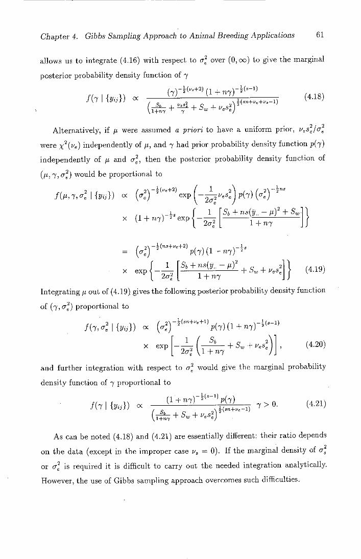
Chapter 4. Gibbs Sampling Approach to Animal Breeding Applications 61
allows us to integrate (4.16) with respect to o- over (0, oo) to give the marginal
posterior probability density function of 'y
fl(lJs+2) (1 + 717)81)
1 vs)+
(4.18)4 s
Sb + + S. + +iv
Alternatively, if p were assumed a priori to have a uniform prior, vs /c
were X 2 (V,) independently of It, and y had prior probability density function p()
independently of p and a, then the posterior probability density function of
(p, y, o- ) would be proportional to
I' 2 f (PI 7,o
>< (1-i
(2 =
(ve+2)
(— 1
2 exp p()
2 (as)
\ _i s f i [ Sb +fl3(Y—P)+sW 717) 2 p1--
1+717
- - (ns+v+2) p(7) (1 + fl7)2
X exp 1 + 717
+ SW + ves (4.19) ]} 1 1 [Sb+ns(y..
)2
Integrating p out of (4.19). gives the following posterior probability density function
of ('y, a) proportional to
f(7, a {y}) cc (2) —(an+u+')
p() (1 + 717)2(81)
L—
(Sb 2a 1 + '
X exp— + + (4.20)
and further integration with respect to a 2 would give the marginal probability
density function of 7 proportional to
(1 + 717)2 p
cc (7)
> 0. (4.21) Sb
f(7 {y})
(_+Sw+ve82 ) \1+n-y e
As can be noted ( 4.18) and (4.21) are essentially different: their ratio depends
on the data (except in the improper case t'3 = 0). If the marginal density of a
or o is required it is difficult to carry out the needed integration analytically.
However, the use of Gibbs sampling approach overcomes such difficulties.

Chapter 4. Gibbs Sampling Approach to Animal Breeding Applications 62
4.2.5 Full conditional distributions of p, {sg}, u and a
The full conditional posterior densities of the parameters of interest are required
to implement the Gibbs sampling approach. The full conditional density of each of
the unknowns is the conditional posterior density regarding all other parameters
in (4.13) as known.
Conditional posterior distribution of gi. The posterior probability density func-
tion (4.13) is proportional in p to
2 ex] {_ [SP - 2pE(Q - sj) 2c i•= 1 Ii
or 1
exp sn [2 - 2p( - )] I -2 U 2 }.
Hence manipulating this leads to the conditional posterior distribution of p given
a and o, which is given by
[p {s}, c, t7, N - s)
Zn ,.1S)
N & , ). 0,
(4.22)
Conditional posterior distribution of s. The posterior probability density func-
tion (4.13) is proportional in the s, to
H[ 8exp [(flu 2 + 2) 2 2n E - )]
I -
i=1
or
11 (n+\ r3 exp
)
- 2na s - P)]
} 2 U.292 L=i flL7 + C
so the s, are conditionally independent given p, u and o with distributions
[s It, a, o, {y}] = N (nc(9. - it) oa
(4.23)
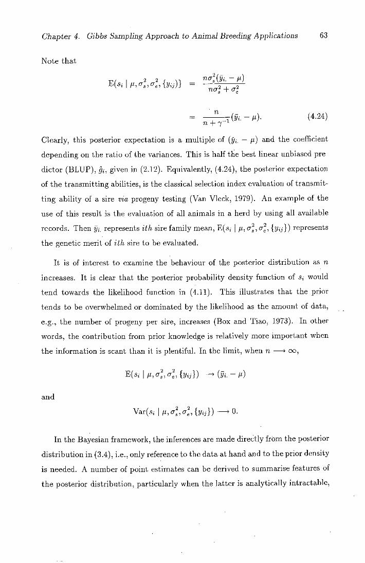
Chapter 4. Gibbs Sampling Approach to Animal Breeding Applications 63
Note that
2 2 E(s fyij)l –
= -1 (4.24)
Th+ -y
Clearly, this posterior expectation is a multiple of (j. — p) and the coefficient
depending on the ratio of the variances. This is half the best linear unbiased pre-
dictor (BLUP), j, given in (2.12). Equivalently, (4.24), the posterior expectation
of the transmitting abilities, is the classical selection index evaluation of transmit-
ting ability of a sire via progeny testing (Van Vleck, 1979). An example of the
use of this result is the evaluation of all animals in a herd by using all available
records. Then jj represents ith sire family mean, E(s 1 p, a, o, {yj}) represents
the genetic merit of ith sire to be evaluated.
It is of interest to examine the behaviour of the posterior distribution as n
increases. It is clear that the posterior probability density function of s i would
tend towards the likelihood function in (4.11). This illustrates that the prior
tends to be overwhelmed or dominated by the likelihood as the amount of data,
e.g., the number of progeny per sire, increases (Box and rriao 1973). In other
words, the contribution from prior knowledge is relatively more important when
the information is scant than it is plentiful. In the limit, when n -i00 )
, a, a, {y}) —# (. — E(s
and
Var(s I L,c,c,{yjj}) —*0.
In the Bayesian framework, the inferences are made directly from the posterior
distribution in (3.4), i.e., only reference to the data at hand and to the prior density
is needed. A number of point estimates can be derived to summarise features of
the posterior distribution, particularly when the latter is analytically intractable,

Chapter 4. Gibbs Sampling Approach to Animal Breeding Applications 64
and probability statements about 9 can be made via without recourse to imaginary
data.
Conditional posterior distribution of a 2 and a. The posterior probability
density function (4.13) is proportional in o to
/ s
(
2 —(s+vs+2) 1 1 ('cc-' 2 2I 3 ) exp (s ± vs. ) I,
\i=1 I]
thus the full conditional posterior distribution of a 2 given i, {s} and c is
S
p,{s},c,{y}J =x2 2
(+8 +u'3s2 8
1=1 1
Similarly the posterior density function (4.13) is proportional in a 2 to
(sm+vc+2) 2 f 1 (Ce)
—5 exp i
1 E(yu - - )
2 + vsl 1,
[i=1 j=1 j J
thus the full conditional distribution of a 2 given p, {s} and c is
(4.25)
5
[Ce I , {s}, 2{yij}] = x2 sn + 'v, ,
E(Yij- s) 2 + e6 I (4.26) i=1 j=i /
It is interesting to observe that the (approximate) marginal posterior densities of
the variance components appear in the inverse x2 form. This conjugate property
of the inverse x2 density can be used to advantage when computing the marginal
density of a variance component from a large data set. The full conditional pos-
terior densities of all unknown parameters (4.22, 4.23, 4.25, 4.26) are essential for
implementing the Gibbs sampling scheme.

Chapter 4. Gibbs Sampling Approach to Animal Breeding Applications 65
4.3 Profile Likelihood
Inference in the presence of nuisance parameters is a widely encountered and
difficult problem, particularly for a frequency-based theory of inference. One of
the simplest approaches is to replace the nuisance parameters in the likelihood
function by their maximum likelihood estimates and examine the resulting profile
likelihood as a function of the parameter of interest. The profile likelihood is then
treated as an ordinary likelihood function for estimation and inference about the
parameter of interest. The procedure is known to give inconsistent or inefficient
estimates for problems with large numbers of nuisance parameters, which suggests
that it may not be close to optimal for a small number of nuisance parameters,
even though the likelihood ratio statistic with no nuisance parameters is in some
sense optimal (Cox and Reid, 1987). Since we want to compare posterior densities
with prior densities and likelihoods, looking at one parameter at a time, we need
a likelihood for each parameter.
Suppose now that we could get a likelihood that does not involve c and 'y. It
is then sensible to look at the likelihood function for
= l(; &2 (p),
(p); {yij})
where &(M) and '5j2) are the maximum likelihood estimates of a and 'y, re-
spectively, for the given value of jt. This is known as the concentrated or profile
likelihood of ji and is equivalent to a sideways view (profile) of the likelihood sur-
face. The profile likelihood may be used to illuminate various aspects of a full
likelihood surface l(p,o,7 I {yj}), for instance by plotting 1 0 (p) against ri. More
importantly, l(ii) can to a considerable extent be thought of and used as if it was
a genuine likelihood. In particular the maximum profile likelihood estimate of it
equals the overall maximum likelihood estimate A.

Chapter 4. Gibbs Sampling Approach to Animal Breeding Applications 66
Suppose after integrating f({yij} I i, {sJ, o, a)f({s} a) over the si ' s
and transforming a to y, the vector of unknown parameters is 01 which can be
partitioned as (i, c, 7) where ji is the parameter of interest and o and 'y are the
nuisance parameters (see Appendix B.1 for the likelihood function of (ii, o, 7)).
Let b i denote (j2,&,j'), the overall maximum likelihood estimate. The likelihood
function for 01 (aside from a multiplicative constant) can be given by
1 3fl r 1 ( B \1
1(01 {y}) () _ 2 (1 + m7) exp
1 + n7)j
+ (4.27)
where
S
B =
= Sb + (v -
5b and S are the sum of squares between and within families, respectively and
are defined in Section 2.3. Hence the log-likelihood is
= --snln(a) - sln(l + n7) - (s +
2 1 +727) (4.28)
and the maximum likelihood estimate of it (for any a and 7) is... Also the
first-order partial derivatives of'o and are
1 2 1 _____ = +
( +
1+727)'
so that
l+fl (4.29) = .572
and
91 li nB ____ 2(l_±n7)+2a (l+ n7 )2
so that
B - (4.30) sue
1+n7(0) -

Chapter 4. Gibbs Sampling Approach to Animal Breeding Applications 67
(4.29) and (4.30) give the following
SW
= s(n - 1)'
so that the profile likelihood of i is
lc(P) =
[
Sw i < . (4.31) s(n —flj
The profile likelihoods of a 2 and 'y can be obtained in the same way. With
= 9, (4.30) gives
, 2 Sb 1 + 7e) = 21
so that the profile likelihood of 0,2 is
2 , 2 — 1 a(n-1) 2 exp (-s) Ct (4.32)
)23 <a <.
With /2 = y.., (4.29) gives
= + S,(1 + 727) ' ] /(sn), (4.33)
so that the profile likelihood for 'y is
(1 + )_43 [s + Sb(1 + 727) - ']
V-0 cc 0 <1/3. (4.34)
Finally the profile likelihood of h 2 can be derived by substituting h 2 /(4 - h 2 ) for
in the log-likelihood function. (4.33) becomes
Sb 1 '2 2 a(h
) = + 1 + (2) i
1(sn) , (4.35)
h2
and the profile likelihood of h 2 can be given by
/ h2 )
I — s[S~
Sb fsn
lc(h 2)[1+n 4h2 +
l+n(-2)j 0h2 l. (4.36)

Chapter 4. Gibbs Sampling Approach to Animal Breeding Applications 68
4.4 Graphical Representation and Gibbs Distri-
bution
Interpreting fitted models with many parameteEs can be difficult. Interpretation
is simplified if we concentrate on the conditional independence structure of the
model. This aspect of the model is most easily presented in the form of a directed
acyclic graph and a conditional independence graph. The purpose of this section
is to demonstrate the use of graphical models as a precise mathematical tool to
represent conditional independence assumptions, especially as a formal language
for communicating causal information in statistical analysis.
Bayesian graphical models provide a link between many different areas of cur-
rent interest. First, computational advances using Markov chain Monte Carlo
methods are becoming more and more popular. Second, complex random effects
models are being increasingly used in a wide variety of applications. Third, graph-
ical representation of conditional independence assumptions is gaining ground in
multivariate analysis (Whittaker, 1990). The graphical representation of multi-
variate distributions is well known in connection with models for high-dimensional
contingency tables (Wermuth and Lauritzen, 1983), for Bayesian inference in ex-
pert systems (Lauritzen and Spiegelhalter, 1988) and for Bayesian frailty models
(Clayton, 1991). Graph theory is also important in the theory of Markov random
fields, which are of considerable importance in statistical mechanics and, more
recently in spatial statistics and image analysis. This theory, reviewed by Geman
and Geman (1984), shows that the algebraic representation of the multivariate
distribution represented by a graph follows from the graph structure; more specif-
ically, it consists of two sets of components, a set of nodes or vertices representing
variables and a set of edges connecting variables and representing association. The
graph structure depends on the set of cliques that makes up the graph, a clique
being a set of nodes in which all pairs are connected. The lack of an edge between

Chapter 4. Gibbs Sampling Approach to Animal Breeding Applications 69
two variables means that the two variables are conditionally independent given the
remaining variables. The joint distribution corresponding to a given conditional
independence graph is proportional to an exponential function of a sum, over all
cliques of potentials where each potential is a function depending on the variables
contained in the corresponding clique (Clayton, 1991). Such a distribution is a
Gibbs distribution.
4.4.1 A graphical representation of the random sire model
The majority of the discussion of graphical models has concerned joint distribution
of observables conditional on a set of unknown parameters, in which the param-
eters and the structure of the independence graph are estimated from data sets
using maximum likelihood. In contrast, since Bayesian inference requires a full
joint distribution for both data and parameters, Bayesian graphical models include
both observed and unobserved quantities within a single graphical structure.
The Bayesian model set out in submodels ((4.2) - (4.6)) incompletely specifies
the joint distribution of the model parameters p, {sJ, a. , a and data. These
submodels merely tie down, a few conditional distributions. To complete the joint
distribution (4.13) of the parameters and data, one seeks some kind of assumption
of independence between the submodels. This is provided by the directed Mar/wv
assumption which simply states that the joint distribution of all the model param-
eters and data is given by the product of all the submodels.
That the directed Markov assumption is natural for model ((4.2) - (4.6)) is
most easily seen from a graph of the model (Figure 4-1), in which round nodes
denote parameters, a rounded rectangle denotes observed data and edges (arrows)
denote dependences specified in the submodels. Figure 4-1 is a directed acyclic
graph for three families si, s and 33 giving data D1 , D2 and D3 since all the
edges are directed and it is not possible, just by following the directions of the
edge, to return to a node after leaving it. In the Bayesian formulation all the
Chapter 4. Gibbs Sampling Approach to Animal Breeding Applications 70
model parameters ft, {s}, c, and c are random variables and the directed graph
represents a conditional argument for parameters conditional on data. if two
parameters are not joined by an edge they are conditionally independent given
the remaining parameters. For example if two variables, U and V, are connected
via a third variable W, then U and V are conditionally independent given W.
Such a set of relationships may also be represented by a conditional indepen-
dence graph, which is an undirected graph. This graph can be constructed from
selected independencies between pairs of variables conditioned on all the remain-
ing variables in a vector of random variables (in some literature the vector of the
remaining variables are referred to as the rest). In such a graph there is no edge
between two vertices whenever the pair of •variables is independent given all the
remaining variables. The conditional independence graph is sometimes called the
moral graph since its structure may be deduced from the directed graph by a
process of marrying the parents (Lauritzen and Spiegelhalter, 1988): if U and V
both have directed links to W in the directed graph, then U and V must be joined
in the (undirected) conditional independence graph. Applying this process to the
directed graph for the random-effect model, Figure 4-1, yields the conditional in-
dependence graph shown in Figure 4-2. This shows, for example, that, conditional
upon the observed data D1 , D2 and D3 , the parameter ji is independent of sj, 32,
33 , c and o.
The Bayesian model described above and illustrated in Figures 4-1 and 4-2
defines a Gibbs distribution with cliques p, s, 82, 33, a, d, D1 , D2, D3 . The
joint probability distribution of the system is proportional to the product of the
priors for jt, {s}, o, and c, and the likelihood function. Bayesian statistical
inference requires computation of joint and marginal posterior distributions of the
parameters given the data. Unfortunately these are intractable, but the condi-
tional distributions are relatively simple. In the next section it will be shown
how this may be exploited in a Monte Carlo method for sampling the posterior
distribution of the parameters.

Chapter 4. Gibbs Sampling Approach to Animal Breeding Applications 71
Figure 4-1: Directed acyclic graph of the Bayesian random effects model for
three families s 1 , S2 and 53 giving the observed data D1 , D2 and D3 .
Figure 4-2: Conditional independence (undirected) graph for the Bayesian ran-
dom effects model for three families 5 1, 2 and .53 giving the observed data D1 ,
and D3.

Chapter 4. Gibbs Sampling Approach to Animal Breeding Applications 72
Denoting conditional probability density distributions by the standard notation
[... I . . .],
the full conditional distributions corresponding to the graph of Figure
4-2 using the joint posterior density function in (4.13) are already given in (4.22),
(4.23), (4.25), and (4.26) for p, {s}, c, and o, respectively.
4.5 Gibbs Sampling
In many Bayesian problems, marginal distributions are needed to make appropri-
ate inferences. However, due to the complexity of joint posterior distributions,
obtaining a high degree of marginalization of the joint posterior density is difficult
or impossible by analytical means. This is so for many practical problems, in-
cluding inferences about variance components. Numerical integation techniques Ae
must be used to obtain the exact marginal distributions, from which function of
interest can be computed and inferences made.
This section describes a numerical integration scheme known as a Monte Carlo
method for generating samples from the joint posterior distribution of the parame-
ters of the model. Use of this method circumvents the analytical problem. At first
sight the method seems to be closely related to bootstrap methods for interval esti-
mation, but there are important differences (Clayton, 1991). Whereas in a frequen-
tist representation of inference problems the unknown parameters are regarded as
fixed constants and the data values are random variables, the Bayesian analysis
reverses the status of the data and parameters: the data are fixed constants and
the parameters are random variables. The frequentist bootstrap regenerates mul-
tiple sets of the data and reanalyses each bootstrapped data set in an attempt to
explore estimation errors. In contrast, a Monte Carlo Bayesian approach holds the
observed data constant, and samples repeatedly from the posterior distribution of
parameters given data.

Chapter 4. Gibbs Sampling Approach to Animal Breeding Applications 73
Recently a number of authors have drawn attention to methods for sampling
multivariate joint and marginal posterior distributions when only conditional dis-
tributions are available. The common feature of these methods is that the sam-
pling is carried out by a stochastic process whose equilibrium distribution is that
required. The idea has its roots in the modification of the Metropolis algorithm
of statistical mechanics. The Metropolis algorithm was developed to investigate
the equilibrium properties of large systems of particles such as molecules in a gas.
However the Gibbs Sampler's wider relevance seems first to have been pointed out
by Hastings (1970) who suggests Markov Chain methods of sampling that gener-
alise the Metropolis algorithm. He illustrates how to use the approach to simulate
Poisson and Normal deviates, as well as random orthogonal matrices. The recent
recognition of its widespread applicability for Bayesian statistical inference follows
the imaginative work of Geman and Geman (1984) in Bayesian image analysis.
They discuss the Gibbs sampler algorithm in the context of spatial procesçin-
volving a way of simulating from high-dimensional complex distributions arising
in image analysis, e.g., image reconstruction. The method consists of iteratively
simulating from the conditional distribution of one variable of the random vector
to he simulated given the current values of the neighbourhood subset of the other
variables. Each complete cycle through the component variables of the vector con-
stitutes one step in a Markov chain whose stationary distribution is, under suitable
conditions, the distribution to he simulated. l3esag (1974) has shown that if the
joint density function is strictly positive over its entire sample space, then the full
joint density is uniquely determined by all full conditional distributions. One of
the basic contributions of Tanner and Wong (1987) was to develop the framework
by which Bayesian computations can he performed in the context of Metropolis
type algorithms.
More recently, Gelfand and Smith (1990) present a comprehensive review of the
Gibbs Sampler and other Monte Carlo methods, such as data augmentation and
the sampling-importance-resampling algorithm. They point out that the Gibbs
Chapter 4. Gibbs Sampling Approach to Animal Breeding Applications 74
Sampler algorithm may be used to simulate from posterior distributions, and hence
may be used to solve standard statistical problems. The use of Gibbs Sampler as
a method for calculating Bayesian marginal posterior and predictive densities is
reviewed and illustrated by Gelfand et al. (1990) with a range of normal data
models, including variance components, unordered and ordered means, hierarchi-
cal growth curves, and missing data in a crossover trial.
The Gibbs Sampler algorithm generates random samples from the Gibbs dis-
tributions which were defined in the previous section. The algorithm visits each
node of a conditional independence graph and generates a value from the full
conditional distribution of the corresponding random variable given the current
values of all its neighbours. Geman and Geman (1984) showed under rather weak
conditions that the resulting sequence of vectors defined on the graph, which is
Markovian, converges to an equilibrium distribution which is the required joint
distribution. This follows regardless of the order in which nodes are visited, pro-
vided each node is visited sufficiently frequently; indeed the algorithm may be
implemented by parallel processing. More usually it is implemented sequentially
by visiting the nodes in a repeated predetermined sequence.
The full conditional distributions presented in Section 4.2.5 are summarised
below:
{Si) ,o,o,{yjj}], normal,
Is i I It, ,c,{yij}], normal and independent,
[o ,{s j },o,{yjj}], inverse x2 ,
[o p, [s}, o, {yj}], inverse x2 •
The ordering placed above is completely arbitrary. The efficient application of
Gibbs sampling depends on two important aspects. Firstly, there must be an
efficient method for generating random samples from univariate or multivariate
conditional posterior distributions. Secondly, as posterior dependence between
parameters can seriously impair the convergence of the procedure to the required
Chapter 4. Gibbs Sampling Approach to Animal Breeding Applications 75
equilibrium distribution, it is helpful if the parameters are approximately indepen-
dent. These two properties ensure that Gibbs sampling is an extremely efficient
method for generating a sample from the posterior distribution of interest. A
further compelling reason for the use of Gibbs sampling, rather than alternative
Markov chain Monte Carlo methods, in the context of animal breeding experi-
ments, is the facility to cope easily with examples in which the data are unbal-
anced. Most commonly, this arises when there are unequal numbers of daughters
per sire. This can easily be dealt with within a Gibbs sampling scheme.
4.5.1 Implementation issues
In this section, the model (4.1) and priors (4.3), (4.4), (4.5) and (4.6) for /2, {s},
c 2 and o, respectively are used to illustrate some implementation issues. Use of
the Gibbs Sampler that ignores the restriction c/c ~ 3 explained in Section 2.4.1
is not sensible at all in animal breeding applications. A solution to this problem
is to adopt a routine that discards values outside certain limits within the Gibbs
sampler process. The sampling algorithm then uses a mixture of Gibbs sampling
algorithm and a routine to discard variances outside the parameter space.
The complete algorithm is as follows.
Given an arbitrary set of starting values, /4(0), cr and for /4, c and
Ole , respectively;
Generate {y} corresponding to half-sib families using model (4.1);
Draw a value 1P from [t I {s} (0) , o 2° o 2 °
, {yjj}] and update z;
(I) 2 ° 2 ° Draw 41) from [s I p ,c3 o , {yjj)} independently and update s (i =
i, ... ,$);
2') Draw o from [o I I(') {}(1). 2 ° , {y j )J and update o;

Chapter 4. Gibbs Sampling Approach to Animal Breeding Applications 76
' () (1)
vi) Draw Ce 2 from [e
2 p 1 , {s} ,
, {y}] and update 0,2;2e;
vii) If 3a 2 ~ cr then repeat v) and vi) until 3c <a;
Thus each variable is visited in the arbitrary order and this cycle completes one
iteration of the sampling scheme. In another words, the first iteration completes a
(0) (0) 2 ° (1) 2@) 2' transition from (p ,s ,c32°
,Ce ) to (p ,s (1) ,o Ce ). The validity of the
Gibbs Sampler stems from the fact that each cycle of the algorithm corresponds
to one step of a Markov chain with stationary transition probabilities and that an
ergodic theorem applies for function under certain regularity conditions (Geman
and Geman, 1984). The values simulated from the posterior distribution can be
obtained in the following three different ways of implementation:
a) A singk long chain : One generates a single run of the Markov chain as
practiced by Geman and Geman (1984) and Besag et al. (1991), i.e.,
viii) Repeat iii)-vii) m times using updated values and store all the values.
If we let the sequence of values for p be p;i, #2, ..., Pin, for example, then
these constitute the simulated values from the marginal posterior distribu-
tionof p. This implementation produces m Gibbs samples (p 1 ,{s 1 },c,c),el
I = l, ... ,m.
b) Equally spaced samples : The second way consists of choosing suitable inte-
gers k and m, performing one long run of a single chainof length km, and
then forming a sample by collecting every kth value, the value of k being
chosen with a view to render serial correlations negligible, i.e.,
viii) Run iii)-vii) km times and store every kth value.
The sample values from the marginal posterior distribution would be P ik,
- ,S), Ck, Ck, I = 1, . . . m where subscript k indicates the kth

Chapter 4. Gibbs Sampling Approach to Animal Breeding Applications 77
iteration or the length of the Gibbs sequence and in is the Gibbs sample
size.
c) Multiple short chains By contrast, Gelfand and Smith (1990) and Gelfand
et al. (1990) have instead performed several runs of each of a number of
independent chains in, forming a sample by collecting the last iterates from
each i.e.,
Run the Gibbs sampler steps iii)-vii) for k iterations and store only the
final state from each.
.
If we let the sample points be p , {s (k) } ( i=1, . . . , s), 2
o (k)
, 2 (k)
% o respectively,
then we would arrive at a joint sample (p (k), {s (Ic) }, 0.2 (k) 2 (k)
) which is a
realization of a Markov chain. Geman and Geman (1984) showed under
suitable regularity conditions that as k -* cc, the points from the kth
iteration are sample points from the appropriate marginal distributions, for
example, p -* p I [p]. Thus for Ic large enough we can regard p as a
simulated observation from [p]. If we independently
Replicate the Ic iterations of i)-viii) in times with different starting
values (using a different random number generator seed each time)
(Ic) (Ic) 2(k) 2(k)
this process would produce miid (s + 3)-tuples A = (pj , {s },c 81 , Oj
1 = 1, . . . ,in.
Let 7r(9) be the equilibrium distribution of the constructed chain. For con-
creteness, suppose that the equilibrium distribution corresponds to a posterior
density
7r(6) = f(A 1 y) ccg(y A)f(A)
which means that the knowledge of the distribution up to proportionality (given
by the likelihood multiplied by the prior) is sufficient for implementation. For
Chapter 4. Gibbs Sampling Approach to Animal Breeding Applications 78
any parameter, the collection of m iid (s + 3)-tuples can be viewed as a simulated
sample from the equilibrium or marginal posterior density given below.
(k) (k) (k)
12 1 ,P2 I f(/1 {yij}) (4.37)
(k) (k) (k)
5 i1 3 i2 ,••'8im f(s {yj}), i = 1,...,s (4.38)
2(k) 2(k) 2(k) 2 a51 'a82 Sm f(a3 {y}) (4.39)
2(k) 2(k) 2(k) 2
Orel 'Ce2 ,, em I {yjj}) (4.40)
The common feature of these implementation methods is that the total number
of samples saved is m. , being the sample size in all. The only difference between
the implementation b) and c) is that in b) there is only one starting value as in
a) whereas in c) there are m different starting values one for each replication. Al-
though the implementation b) lessens the dependence on initial values a potential
disadvantage of it is that the Gibbs sequence may stay in a small subset of the
sample space for a long time. The choice between different ways of implementing
the Gibbs sampler algorithm has not been settled. In the first two ways a) and
b), the starting point for every subsequence of length Ic is closer to a draw from
the stationary distribution than the corresponding starting point in the third way,
which is chosen by the user (Raftery and Lewis, 1992).
Gelman and Rubin (1992a), on the other hand, have argued that one single
long run approach may appear to be more efficient in that only one transient
phase is involved. However, it can be disputed that monitoring the evolutionary
behaviour of several runs of the chain starting from a wide range of initial values
is necessary. The essence of their argument is that it is not possible to know, in
the case of any individual problem, whether a single run has converged, and that
combining the results of runs from several starting points gives an honest, if not
conservative, assessment of the underlying uncertainty.
In either case, a key problem is to decide how long the chain should be run for,
and whether this can be done in advance or needs to be determined by some kind
Chapter 4. Gibbs Sampling Approach to Animal Breeding Applications 79
of sequential stopping rule. Examining several successive batches within a single
run can certainly provide (negative) evidence that a run is not sufficiently long
(Smith and Roberts, 1993). However, there can never be any (positive) empirical
guarantee that a sufficiently long run has been taken.
It has been common practice when running the Gibbs sampler to throw away
a substantial number of initial iterations, often on the order of 1,000. Raftery and
Lewis (1992) suggested that this might not usually be necessary, and indeed, could
often be quite wasteful. It has also been common practice to use implementations
b) and c) (especially b) storing only every kth, usually 10th or 20th, iterate and
discarding the rest. The results of Raftery and Lewis (1992) showed that in many
cases this is rather profligate. Indeed, in some cases, the dependency between suc-
cessive iterates is weak and it makes sense to use them all, even when storage is an
issue. By contrast to Gelman and Rubin (1992a), they recommended that Markov
chain Monte Carlo inference ultimately be based on a single long run, but that
this be monitored using carefully chosen diagnostics, and that the starting values
and the exact form of the algorithm be chosen on the basis of experimentation.
Based on theoretical arguments by Gelman and Rubin (1992a) and on our
experience, the single long-chain method of implementing Gibbs sampler is a pre- 2
ferred method in this thesis. Since interest centres on making inferences about a,
cr and their functions, less attention will be paid hereafter to It and .s. However,
it is clear that the marginal distributions of M and si are also obtained as a byprod-
uct of Gibbs sampling. Later in this chapter, all three implementation methods
will be compared since the best method presumably depends on the particular
problem.
4.5.2 Assessing convergence
The Gibbs sampling method is not complete without a determination of the length
of Gibbs sequence, k, and across iterations, a specification of the Gibbs sample
Chapter 4. Gibbs Sampling Approach to Animal Breeding Applications 80
size, in. It is indeed fact that the Gibbs sampler can be extremely computationally
demanding, even for relatively small-scale statistical applications, and hence it
is important to know how many iterations are required for any individual data
application or any individual parameter to achieve the desired level of accuracy.
Appropriate values required for k and in vary considerably depending upon the
particular application and what is being approximated, and cannot be specified
a priori. A general strategy for choosing such k is to monitor the convergence of
some aspect of the Gibbs sampling.
From a practical viewpoint, one requires a rule telling where to stop the algo-
rithm, hopefully at a time when equilibrium has been reached, or 'convergence'
achieved. Convergence expresses the idea that the current iteration has been
drawn from a distribution, 'close' in some sense to the stationary distribution.
Although several methods have been proposed for assessing convergence of the
Gibbs sampler, results of some theoretical literature do not easily translate into
clear guidelines for the Bayesian practitioner. It is beyond the scope of this thesis
to discuss the mathematical details of these methods. The following gives a sum-
mary discussion of various methods of output analysis (convergence diagnostics).
Gelfand and Smith (1990) and Gelfand et al. (1990) perform multiple parallel
runs (implementation c) of Section 4.5.1 and graphically compare resulting cross-
run posterior densities at each of several iterations. They monitor the generated
data in a univariate fashion, allowing the sampler to run until the marginal pos-
terior distributions for each parameter of interest appear to have converged. For
a fixed in they increase It, overlay plots of the resulting estimated densities (4.41),
see if the estimates are visually indistinguishable. Similarly, they also increase in
to assess stability of the density estimate. They hold in somewhat small (often as
small as 25 and at most 200) until convergence is indicated, at which point, for a
final iteration, they typically increase in by an order of magnitude to obtain the
density estimate (4.41).

Chapter 4. Gibbs Sampling Approach to Animal Breeding Applications 81
Raftery and Lewis (1992) describe an easily-implemented method for deter-
mining the total number of iterations required, and also the number of initial
iterations that should be discarded to allow for burn-in. The burn-in or warm-up
problem is the question of how much of a run should be thrown away on grounds
that the chain may not yet have reached equilibrium. They argue that as a prac-
tical matter, it is desirable to run the Gibbs sampler for the smallest number
of iterations necessary to attain a required level of accuracy. The method uses
only the Gibbs iterates themselves, and does not, for example, require external
specification of characteristics of the posterior density. They consider the specific
problem of calculating particular quantiles of the posterior distribution of a func-
tion U of the parameter 0. Suppose that F[U < u I y] is to be approximated to
within +r with probability .s. The approximate number of iterations required is
found to do this when the correct answer is q. For example, if q = .025, r = . 005
and .s = .95, this corresponds to requiring that the cumulative distribution func-
tion of the .025 quantile to be estimated to within +.005 with probability .95.
This method returns the number, M, of initial iterations to be discarded (burn-in
iterations), the number, N = km, of additional iterations required, and Ic, where
every Icth iterate is used. The problem with this method is that the result is by
far the most sensitive to the value of r, since N = r 2 . It is also difficult to specify
the value of r as this depends on the type of distribution and it is not known
in advance how heavy the posterior tail is. As r increases the total number of
iterations N decreases dramatically, but M and Ic remain unchanged. Hence the
method can be effectively used to determine only M and Ic.
Roberts (1992) develops an integral norm for assessing convergence of multiple
runs of a symmetrised Gibbs sampler. Geweke (1992) calculates an arbitrary
function of the parameters at each iteration of a single run of the Gibbs sampler.
This arbitrary function could for example be a single model parameter. Two
moving windows are defined, the first towards the start of the series and the

Chapter 4. Gibbs Sampling Approach to Animal Breeding Applications 82
second including the most recent iteration. Nonconvergence is indicated if the
function departs significantly from a standard normal deviate.
Gelman and Rubin (1992a) argued that convergence cannot reliably be as-
sessed on the basis of one run of the Gibbs sampler. They advocate using several
parallel runs with widely dispersed starting values, calculating an arbitrary uni-
variate function of the parameters at each iteration in each run. By comparing
between- and within-run sums of squares for the function, they estimate a scale
reduction factor and a conservative estimate of its 97.5% ceultile (Gelman and Ru-
bin, 1992b). The scale reduction factor estimates 110w much the observed variance
in the function might be reduced if Gibbs sampling was continued indefinitely; a
scale reduction factor of 1.0 indicates no reduction, and hence convergence. How-
ever, this method necessarily suffers from the deficiency of possibly overlooking
lack of convergence of some aspect of the distribution.
4.5.3 Absorbing state
Sampling the joint posterior distribution of parameters by stochastic substitution
such as Gibbs sampling can be relatively easy to implement. However, it is some-
times possible to encounter a serious difficulty with the Gibbs sampling scheme in
that there is an absorbing state when the prior information is sufficiently diffuse
(e.g. v3 = 0 defines an absorbing state in model (4.1)). If the prior degrees of
freedom, v3 , for the sire variance component, or, 2 , is close to zero, then the algo-
rithm gets stuck periodically in a vicious circle for several hundred iterations at a
time creating computational black holes from which no single-component updating
scheme can escape; see for example, the spatial epidemiology application in Be-
sag et ad. (1991) or random effects proportional hazards model of Clayton (1991).
Single-run diagnostics for the random effects variance will reveal this immediately,
but the series for other quantities such as the random effects themselves, s, can be
almost unrelated and give no hint of trouble. In practice, therefore, the absorbing
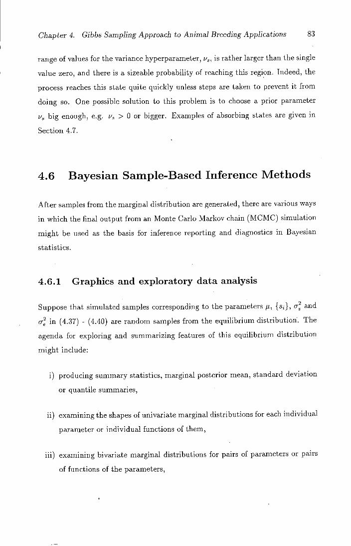
Chapter 4. Gibbs Sampling Approach to Animal Breeding Applications 83
range of values for the variance hyperparameter, u 8 , is rather larger than the single
value zero, and there is a sizeable probability of reaching this region. Indeed, the
process reaches this state quite quickly unless steps are taken to prevent it from
doing so. One possible solution to this problem is to choose a prior parameter
v3 big enough, e.g. v3 > 0 or bigger. Examples of absorbing states are given in
Section 4.7.
4.6 Bayesian Sample-Based Inference Methods
After samples from the marginal distribution are generated, there are various ways
in which the final output from an Monte Carlo Markov chain (MCMC) simulation
might be used as the basis for inference reporting and diagnostics in Bayesian
statistics.
4.6.1 Graphics and exploratory data analysis
Suppose that simulated samples corresponding to the parameters p, {sJ, a and
a in (4.37) - (4.40) are random samples from the equilibrium distribution The
agenda for exploring and summarizing features of this equilibrium distribution
might include:
producing summary statistics, marginal posterior mean, standard deviation
or quantile summaries,
examining the shapes of univariate marginal distributions for each individual
parameter or individual functions of them,
examining hivariate marginal distributions for pairs of parameters or pairs
of functions of the parameters,

Chapter 4. Gibbs Sampling Approach to Animal Breeding Applications 84
examining trivariate distributions,
uses of the output for specific decision problems or predictive analysis.
The posterior mean and standard deviation are often used to provide a summary of
the posterior distribution. From a decision theoretical point of view, the optimum
Bayes estimator under quadratic loss is the posterior mean; the posterior median
is optimal if the loss function is proportional to the absolute value of the error of
estimation and the posterior mode is optimal if a step loss function is adopted. A
robust measure of location, such as the median, may be preferable to the posterior
mean as a descriptive measure, and the median is a quantile. Also, the posterior
standard deviation is often used as a way of obtaining an approximate confidence
interval if the posterior distribution is roughly Normal.
Point estimates of variance components, e.g., mean, mode and median will
always be within the parameter space. Likewise, interval estimates are also within
the parameter space, in contrast to the asymptotic confidence intervals obtained
from full or restricted maximum likelihood, which may include negative values.
It is interesting to notice that much of this agenda of exploration and sum-
marization is very much the same as presents itself when one is interested in ex-
ploratory data analysis (EDA) of a point cloud of multivariate observations (Smith
and Roberts, 1993). The individual observation vectors are here replaced by the
individual parameter vectors drawn from the posterior; the number of observa-
tions corresponds to the size of the sample drawn from the posterior. It follows
that the exploratory, particularly graphical, toolkit developed by the multivariate
EDA and visual EDA communities now finds an additional role as an essential
part of the Bayesian computational toolkit (Smith and Roberts, 1993).
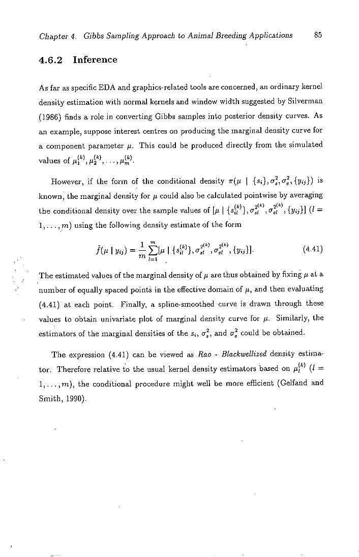
Chapter 4. Gibbs Sampling Approach to Animal Breeding Applications 85
4.6.2 Inference
As far as specific EDA and graphics-related tools are concerned, an ordinary kernel
density estimation with normal kernels and window width suggested by Silverman
(1986) finds a role in converting Gibbs samples into posterior density curves. As
an example, suppose interest centres on producing the marginal density curve for
a component parameter IL. This could be produced directly from the simulated
values of ) f4, (k) ,
However, if the form of the conditional density ir(p I {s 1 ),a 7 c, {y}) is
known, the marginal density for z could also he calculated pointwise by averaging
the conditional density over the sample values of [p I {s {y}] (1 =
I.... ,rn) using the following density estimate of the form
1 (k) 2(k)
I y) = L >[ I {s, }, &8 1 ,o 1 , {yjj}]. (4.41)
The estimated values of the marginal density of t are thus obtained by fixing p at a
number of equally spaced pointá in the effective domain of it, and then evaluating
(4.41) at each point. Finally, a spline-smoothed curve is drawn through these
values to obtain univariate plot of marginal density curve for p. Similarly, the
estimators of the marginal densities of the s, a, and a could be obtained.
The expression (4.4.1) can be viewed as Rao - Blackwellized density estima-
tor. Therefore relative to the usual kernel density estimators based on p (1 =
1,... On), the conditional procedure might well be more efficient (Gelfand and
Smith, 1990).

Chapter 4. Gibbs Sampling Approach to Animal Breeding Applications 86
4.7 A Simulation Study of a Balanced Sire Model
4.7.1 Preliminary results
Four sets of data were generated for a single trait from random normal deviates
based on a one-way sire model in (4.1) with equal numbers, it of offspring per sire.
In all simulations, parameter values used were ji = o, a 2 = 0.025, or2 = 0.975 and
hence h 2 = 0.1. The number of sire families, s, is 25 while number of progeny per
sire, it, is 20. We feel that these four data sets with 200 observations available
cover the majority of situations where the one-way half-sib model is appropriate.
For, example, there is a fairly wide range of heritability estimates, including a
negative one.
Analysis of variance (ANOVA) is carried out for each data set. The resultant
sum of squares and mean squares are summarised in Table 4-1 and the ANOVA
estimates are given in Table 4-2. As can be seen from this table data sets yield
ANOVA estimates of heritability ranging from -0.0732 to 0.3058. The second and
most difficult data set is badly behaved, in that the standard estimate of a is
negative, rendering inference about o difficult.
For illustrative purposes, Bayesian analyses based on the prior specification
= 0.025 and 82 = 0.975 with varying values of v3 and e, a) v3 = = 0,
b) v3 = ii, = 0.5 and c) v3 =v,= 1 are provided for all data sets. Under this
specification, we have weak independent inverse x2 priors for o 2 and o. The
sample data provide very little information about a as there are only 25 sires.
The implementation of the Gibbs Sampler algorithm is carried out for the four
sets of data in the following ways:
a) A single run of 1,000 Gibbs Sampler iterations.

Chapter 4. Gibbs Sampling Approach to Animal Breeding Applications 87
Table 4-1: ANOVA tables of four data sets generated using s = 25, n = 20,
= 0, T = 0.025 and a = 0.975
Source df 55 MS
Data Set 1
Between sires 24 67.2697 2.8029
Within sires 475 501.3577 1.0555
Total 499 568.6274
Data Set 2
Between sires 24 15.4126 0.6422
Within sires 475 476.0895 1.0023
Total 499 491.5021
Data Set 3
Between sires 24 38.0346 1.5848
Within sires 475 481.2948 1.0133
Total 499 529.3294
Data Set 4
Between sires 24 29.2666 1.2194
Within sires 475 458.7445 0.9658
Total 499 488.0111

Chapter 4. Gibbs Sampling Approach to Animal Breeding Applications 88
Table 4-2: ANOVA estimates for the four data sets.
Data sets Y 9 2 or -y h 2
1 -0.0248 0.0874 1.0555 0.0828 0.3058
2 0.0721 -0.0180 1.0023 -0.0180 -0.0732
3 0.0400 0.0286 1.0133 0.0282 0.1097
4 -0.0318 0.0127 0.9658 0.0131 0.0518
Picking off every i) 10th, ii) 20th and iii) 30th value in a single long run of
length 10,000, 20,000 and 30,000, respectively, using only one starting value
for each parameter.
Short runs of Gibbs Sampler steps of length i) 10, ii) 20 and Hi) 30, storing
the last iterate and replicating this process 1,000, 2,000 and 3,000 times,
respectively, using different starting values each time
Summaries of the resulting marginal posterior densities for p, o, o, 'y and h 2 are
shown in Table 4-3. Marginal posterior means and standard deviations calculated
from the four data sets in this table are based on 1,000 Gibbs samples using the
three different ways in which the algorithm is implemented. This table reveals
that there is little difference between the ways of implementation since marginal
posterior means and standard deviations for the three implementation seem to
be very close for each data set. Therefore, one does not get an appreciably bet-
ter answer by throwing away some of the iterations and for further analysis and
investigations the implementation a) will be used to make inferences about the
parameters of interest. The results of Raftery and Lewis (1992) agree with the
conclusion drawn here.
Using a density estimator with normal kernels and window width suggested by
Silverman (1986) based on subsequent samples of 1,000, Figures 4-3-4-8 represent
the curves corresponding to the marginal posterior densities for jt, {s}, a, c, 7

Chapter 4. Gibbs Sampling Approach to Animal Breeding Applications 89
Table 4-3: Marginal posterior mean and standard deviation (SD) of parameters
for four data sets based on 1,000 Gibbs samples for different prior degrees of
freedom v 8 and v5 and three ways of implementing the Gibbs Sampler.
Implementation a)
0.0 -00313 0.0801 0.0898 0,0428 1.0622 0,0706 0.0852 0.0415 0.3089 0.1364
0.5 -0.0314 0.0805 0.0917 0.0429 1.0628 0.0705 0.0869 0.0416 0.3147 0.1362
1.0 -0,0272 0.0715 0.0861 0.0407 1.0625 0.0704 0.0815 0.0389 0.2969 0.1268
Implementation b(i)
0.0 -0.0261 0.0731 0.0877 0,0425 1.0635 0.0680 0.0832 0,0416 0.3019 0.1369
0.5 0.0262 0.0736 0.0897 0.0427 1.0639 0.0679 0.0850 0.0418 0.3081 0.1367
1.0 -0.0217 0.0777 0.0843 0.0426 1,0608 0.0694 0.0799 0.0406 0.2908 0.1349
Implementation C (i)
0.0 -0,0251 0,0745 010905 0,0453 1,0616 0.0717 0.0860 0,0442 0,3110 0.1446
0,5 -0,0244 0,0804 0,0916 0,0453 1.0647 0,0660 0.0867 0,0436 0.3133 0.1428
1.0 -0,0217 0.0713 010826 0,0413 1.0661 0,0725 0,0782 0,0404 0,2851 0.1335
Implementation b(ii)
0,0 -0,0251 0.0728 0,0903 0,0444 1.0636 0,0704 0.0857 0,0435 0,3100 0.1420
0,5 -0,0252 0.0733 0,0923 0,0444 1.0641 0,0704 0,0875 0,0435 0,3162 011404
1.0 -0,0257 0,0768 0,0847 0,0430 1,0603 0,0666 0.0803 0.0411 0,2921 0.1357
Implementation c(ii)
0,0 -0.0240 0,0764 0,0917 0,0473 1,0637 0,0689 0,0869 0,0454 0,3135 0,1473
0,5 -0.0241 0.0793 0,0950 0,0481 1,0631 0,0704 0,0899 0,0460 0,3238 0,1482
1,0 -0.0223 0,0734 0,0822 0,0410 1,0650 0,0706 0,0778 0,0397 0,2839 0,1321
Implementation b(iii)
0.0 -0.0247 0,0749 0.0877 0,0451 1,0637 0,0696 0.0831 0,0439 0.3011 0.1430
0.5 -0,0247 0,0754 0,0897 0,0451 1,0641 0,0696 0.0850 0,0439 0.3076 0.2423
1.0 -0,0237 0,0781 0,0828 0.0406 1,0651 0,0692 0.0783 0,0390 0.2857 0,1208
Implementation c(iii)
0.0 -0.0257 0,0739 0.0919 0,0466 1,0618 0,0678 0.0871 0,0445 0,3147 0,1447
0.5 -0.0248 0,0755 0,0932 0.0457 1,0659 0.0704 0.0880 0,0443 0,3178 0,1430
1.0 -0.0257 0,0763 0,0850 0.0431 1,0634 0,0689 0.0806 0.0417 0,2929 0,1383
DATA SET 2
Implementation a)
0,0 0,0706 0.0478 0,0012 0,0038 0,9881 0.0641 0,0012 0.0039 0.0047 0,0152
0.5 0,0701 0,0517 0.0104 0,0080 019878 0,0642 0.0106 0.0082 0,0415 0,0316
1,0 0,0712 0.0489 0.0119 0,0079 0,9868 0,0636 0,0121 0.0079 0,0477 0.0306
Implementation b(i)
0,0 0,0734 0.0454 0.0009 0,0030 0.9896 0.9632 0.0009 0,0032 0,0035 0.0124
0.5 0,0739 0.0498 0.0108 0,0078 0.9895 0,0631 0.0110 0,0080 0,0433 0,0309
1.0 0,0724 0.0494 0.0117 0.0077 0.9879 0,0629 0.0119 0.0080 0.0467 0,0306
Implementation c(i)
0.0 0.0731 0.0434 0,0004 0,0019 0.9889 0,0621 0,0004 0.0019 0.0014 0,0076
0,5 0,0706 0,0501 0,0106 0,0086 0,9898 0.0616 0-0108 0,0087 0,0424 0.0335
2,0 0,0708 0,0501 0,0115 0.0079 0,9861 0,0631 0,0117 0,0081 0,0461 0.0311
Implementation b(ii)
0,0 0.0734 0,0451 0,0005 0.0022 0.9898 0.0641 0.0005 0,0023 0,0019 0,0091
0.5 0,0731 0,0493 0,0108 0.0083 019899 0,0642 0.0110 0,0085 0.0432 0,0325
1,0 0,0722 0.0494 0,0117 0.0078 0,9869 0,0614 0.0119 0.0079 0,0467 0,0306
Implementation c(ii)
0,0 0,0739 0,0467 0,0002 0,0014 0,9878 0.0612 0.0002 0,0015 0,0006 0,0059
0.5 0,0716 0.0489 0.0113 0,0088 0,9889 0.0630 010115 0,0090 0,0450 0,0347
1.0 0.0702 0.0501 0,0118 0,0082 0,9855 0,0621 0,0120 0,0083 0,0471 0,0318
Implementation b(iii)
0.0 0,0733 0,0452 0.0004 0,0018 0,9888 0,0672 0,0004 0.0018 0.0016 0.0071
0,5 0.0745 0,0507 0,0108 0,0078 0,9886 0,0673 0,0110 0,0080 0,0432 0.0307
1,0 0,0719 0.0502 0,0117 0,0079 0,9837 0,0628 0,0120 0,0083 0,0472 0,0317
Implementation c(iii)
0,0 0,0735 0.0435 0.0001 0.0007 0.9931 0,0634 0,0001 0,0007 0,0004 0,0026
0.5 0.0714 0.0496 0,0206 0,0080 0.9890 0,0658 0,0108 0,0082 0,0423 0,0317
3.0 0,0694 0.0482 0,0117 0,0079 0,9880 0,0651 0,0119 0,0082 0.0468 0.0316

Chapter 4. Gibbs Sampling Approach to Animal Breeding Applications 90
Marginal posterior mean and standard deviation (SD) of parameters for four data
sets based on 1,000 Gibbs samples for different prior degrees of freedom v 3 and v6
and three ways of implementing the Gibbs Sampler, continued from Table 4-3...
Implementation a)
0,0 0,0377 0.0544 0.0130 0.0198 1.0330 0.0685 0.0128 0,0198 0.0493 0.0738
0.5 0.0369 0.0610 0.0332 0.0227 1.0187 0.0673 0.0329 0,0227 0.1256 0.0825
1,0 0.0390 0.0553 0,0288 0.0191 1.0200 0.0670 0.0284 0,0188 0.1093 0.0695
Implementation b(i)
0,0 00410 0.0505 0.0093 0.0182 1,0381 0.0670 0.0091 0.0181 0.0349 0.0677
0,5 0.0421 0.0588 - 0.0325 0.0227 1.0217 0.0665 010321 0.0227 0.1226 0.0820
1,0 0.0406 0.0589 0.0296 0.0208 1.0205 0.0664 010293 0.0209 0.1121 0.0763
Implementation c(i)
0.0 0,0408 0.0507 0,0099 0,0175 1.0374 0.0657 0,0097 0,0172 0.0375 0.0650
0.5 0.0376 0,0577 0.0350 0,0244 1.0226 010669 0.0345 0.0244 0,1313 0.0884
1.0 0,0399 0,0573 0,0303 0,0215 1.0209 0,0640 0.0300 0.0217 0.1148 0,0792
Implementation b(ii)
0.0 0.0402 0.0494 0.0071 0.0152 1.0397 0,0686 0.0070 0.0152 0.0268 0,0575
0.5 0.0411 0.0583 0.0328 0.0243 1.0219 0,0682 0.0324 0.0244 0.1235 0,0882
1.0 0.0398 0.0569 0.0294 0.0199 3,0195 0,0647 0,0290 0.0198 0.1115 0.0729
Implementation c(H)
0.0 0.0390 0.0476 0.0040 0,0122 1.0409 0.0635 0,0039 0.0123 0.0150 0.0463
0.5 0,0368 0.0599 0,0335 0,0249 1,0189 0.0678 0.0333 0.0253 0.1266 0,0911
1.0 0,0381 0.0565 0,0281 0.0194 1,0219 0,0684 0.0277 0,0193 0,1065 0,0708
Implementation b(iii)
0.0 0,0417 0.0494 0,0068 0.0156 1.0389 0,0710 0.0067 0.0155 ' 0.0257 0.0584
0.5 0,0430 0.0597 0,0327 0.0230 1,0205 0.0706 0.0323 0.0231 0,1234 0,0840
1.0 0,0390 0.0576 0,0295 0.0198 1.0156 0.0661 0,0294 0,0202 0,1127 0.0742
Implementation c(iii)
0,0 0.0420 0.0468 0.0049 0.0143 1,0370 0.0692 0,0048 0,0142 0.0184 0.0534
015 0.0414 0,0578 0.0318 0,0230 1.0242 0,0671 0.0314 0.0230 0.1197 0.0835
110 0.0420 0,0576 0.0289 - 0,0202 1.0214 0,0669 0.0286 0.0204 0.1097 0.0744
DATA SET
Implementation a)
0.0 -0.0336 0,0499 0,0051 0,0097 0.9773 0.0638 0,0053 0,0100 0,0207 0.0387
0.5 -0.0340 0.0549 0,0196 0,0153 0.9688 0.0632 0,0204 0,0160 0,0789 0,0601
1.0 -0.0324 0.0508 0.0182 0,0127 0.9690 0.0626 0.0189 0.0132 0.0736 0.0498
Implementation b(i)
0.0 .0 0307 0.0465 0.0034 0.0094 0.9804 0.0629 0.0035 0.0098 0.0136 0.0374
0.5 '0.0299 010536 0.0207 0,0360 0.9702 0.0626 0.0216 0.0169 0.0834 0.0630
1.0 '0.0313 0.0540 0.0198 0.0148 0.9686 0.0620 0.0206 0.0154 0.0798 0.0575
Implementation c(i)
010 .0.0299 0.0424 0.0022 0.0076 0.9756 0,0624 0.0023 0.0080 0.0088 0.0304
0.5 -0.0316 0.0531 0.0215 0.0167 0.9669 0.0599 0.0224 0.0175 0.0865 0.0652
1.0 -0.0344 0.0522 0.0207 0.0144 0.9664 0,0627 0.0216 0.0153 0,0838 0.0572
Implementation b(ii)
0.0 -0.0309 0.0459 0.0019 0.0066 0.9814 0.0639 0.0020 0.0070 0,0076 0,0267
0.5 -0.0312 0.0530 0.0211 0.0164 0.9701 0.0642 0.0220 0.0172 0.0849 0.0640
110 '0.0318 0,0525 0,0201 0.0145 0,9678 0,0606 0.0209 0.0152 0,0809 0,0571
Implementation c(ii)
0,0 -0.0320 0,0456 0.0029 0,0094 0,9796 0.0614 0,0031 0,0099 0.0119 0.0370
0.5 '0,0356 0,0522 0.0206 0.0172 0.9698 0,0612 0.0214 0,0183 0.0828 0.0676
1.0 -0,0323 0.0516 0.0203 0.0150 0.9674 0,0630 0.0210 0.0156 0.0815 0.0582
Implementation b(iii)
0.0 '0.0307 0,0461 0.0021 0.0074 0.9803 0.0667 0,0022 0.0077 0.0086 0.0296
015 -0.0288 - 0.0547 0-0212 0,0160 0.9688 0.0665 0.0221 0.0167 0.0853 0.0625
1,0 -0.0325 0.0538 0.0202 0.0145 0.9640 0.0617 0.0212 0,0155 0,0820 0.0578
Implementation c(iii)
0.0 .0,0326 0,0450 0,0012 0.0059 0.9783 0,0610 0.0013 0,0062 0,0051 0.0238
0.5 '0.0331 0.0526 0.0211 0.0171 0,9696 0.0626 0.0219 0.0179 0.0844 0.0666
1.0 '0.0346 0.0515 0.0205 0.0146 0,9661 0.0626 0.0214 0.0156 0.0830 0.0583
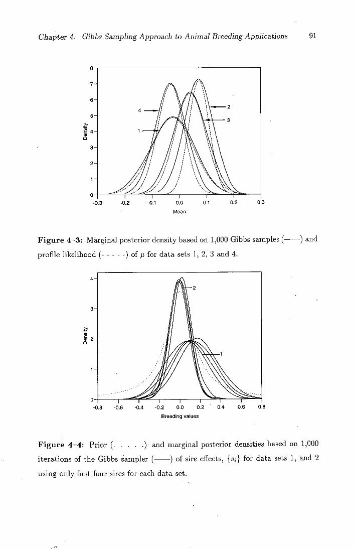
Chapter 4. Gibbs Sampling Approach to Animal Breeding Applications 91
0) C ci) a
6-
A
6- / / \ 4
2 —:
5-
4-
/
3- •1 / / 2-
0 - ----- -,
Is -0.2 -0.1 0.0 0.1 0.2 0.3
- Mean
Figure 4-3: Marginal posterior density based on 1,000 Gibbs samples ( ) and
profile likelihood (- - - - -) of ti for data sets 1, 2, 3 and 4.
4-
2
3-
0 C a, C
Breeding values
Figure 4-4: Prior (.....)- and marginal posterior densities based on 1,000
iterations of the Gibbs sampler ( ) of sire effects, {s} for data sets 1, and 2
using only first four sires for each data set.

Chapter 4. Gibbs Sampling Approach to Animal Breeding Applications 92
0] C C a
0.0 0.05 0.1 0.15 0.2
Sire variance component
Figure 4-5: Prior (.....) and marginal posterior densities based on 1,000
Gibbs samples ( ) of C2 for four sets of data.
0 C a a
0.0 0.2 0.4 0.6 0.8 1.0 1.2 1.4 1.6
Residual variance component
Figure 4-6: Prior (.....) and marginal posterior densities based on 1,000
iterations of the Gibbs sampler ( ) and profile likelihood (-----) of c for
data sets 1, 2, 3 and 4.

Chapter 4. Gibbs Sampling Approach to Animal Breeding Applications 93
0 C 0 0
0.0 0.05 0.1 0.15 0.2
Gamma
Figure 4-7: Prior (.....) and marginal posterior densities based on 1,000
Gibbs samples ( ) and profile likelihood (-----) of -y for four sets of data.
6-
4-
2 - -
_ 2
C 8- 0 0
6- \
4- /\ 3
/ --
2- 1 --- - - --
0- •
>c
Heritability
Figure 4-8: Prior (.....) and marginal posterior densities based on 1,000
Gibbs samples ( ) and profile likelihood (-----) of h 2 for data sets 1, 2, 3
and 4.

Chapter 4. Gibbs Sampling Approach to Animal Breeding Applications 94
and h2 , respectively. Profile likelihoods for i, a, 'y and h 2 and prior densities for
22 a, o- , 'y and h 2 are also illustrated in these figures. The marginal posterior
densities seem to tell us more than the profile likelihoods, especially for 'y and h 2 in
Figures 4-7 and 4-8. Moreover there is a noticeable difference between the curves
of the marginal posterior densities and of the profile likelihoods in Figures 4-7 and
4-8. In general the profile likelihood of each parameter appears more concentrated
than the posterior density; the latter reflects the uncertainty in other parameters.
To summarise our conclusion so far, point estimates of variance components
from Bayesian analysis are within the permissible parameter space in contrast
to the estimates obtained from ANOVA. The Bayesian method is feasible com-
putationally and appears to give much more sensible answers to the inferential
problems than maximum likelihood estimation. Our task now is to explain this
discrepancy, and to investigate the reason behind it.
Convergence assessment
The Gibbs sampler is run using the three implementation methods described in
4.7.1, each giving an ultimate Gibbs sample size of 1,000. However the implemen-
tation a) is chosen for further analysis and, investigations. Figure 4-9 illustrates
the values for each of the model parameters, 1L, o, o, 'y and h 2 for the first 300
iterations from the implementations a) and c) of the Gibbs sampler for data set 1
when 1/3 = ii = 1.
Applying Gelfand et al. (1990) and Raftery and Lewis's (1992) convergence
criterion separately to each of the model parameters showed that convergence in
distribution had been achieved by iteration 1,000 (Figure 4-9). The marginal
posteriors from the implementation b) (not shown in Figure 4-9 were virtually
identical to those from the implementations a) and c). For all parameters, t,
'y and I2 the convergence appears to have been achieved within 100 iterations.
In fact, Gelfand et al. (1990) described a method under different values of k and m,

Chapter 4. Gibbs Sampling Approach to Animal Breeding Applications 95
and suggested using k = 10-20 and rn = 100 (for implementation c)) for a variance
component problem in a balanced one-way model. This means that their final
Gibbs sample size was 100 which was enough for a good convergence. However,
they increased in to 1,000 when the variance ratio was under consideration. The
numerical results of this work for the same model support their suggestion. Wang
et al. (1993) using the same model also agreed with the results of Gelfand et al.
(1990) for the value of k, but indicated that Gibbs sample sizes of 2,000 to 3,000
may be needed for badly behaved marginal distributions in that 'y = 0.01. Wang
et al. (1993) reported that in general the appropriate values of k and in depend on
the number of parameters in the model, the shapes of the marginal distributions
and the accuracy required to estimate densities.
Raftery and Lewis's (1992) convergence criterion was applied to determine the
number of burn-in iterations (transition phase), M, and the length of the Gibbs
Sampler sequence, k or the kth iteration. To implement their method only the
required precision, as specified by the four quantities q, r, s and c is needed, where
c is the error in the cumulative distribution function at the quantile. The typical
values of q = . 025, r = . 005, .s = .95 and e = .001 were chosen for each parameter.
In our simulated four examples the method gave k = 1 and M = 2 - 3 which is a
very small number of burn-in iterations for all parameters when v was 0.5 and 1.
This amount of burn-in is negligible. Ic = 1 suggests that the level of dependence
between the Gibbs sampling iterates is not very high (Figure 4-9), and thus that
the sampler is rather fast to convergence to the desired distribution.
The data set 2 which experiences computational black holes when v3 = 0
is chosen for detailed investigation of convergence assessment using Raftery and
Lewis's (1992). method. The parameters i and or gave the same results for k
and M as above, regardless of the value of v 8 . However different values of Ic
and M are obtained for the parameter a using different implementations of the
Gibbs sampler with v3 = 0; for implementation a) Ic = 5 and M = 1070, for
implementation b) Ic = 2 and M = 132 and for implementation c) Ic = 1 and M =
C
a 8
2 CI,
Iteration
250 300
0.0
-0.1
-0.2
-0.3
0 150
Iteration
a)
a a 8
Ct
Cr
0 50 100 150 200 250 300
Iteration
Chapter 4. Gibbs Sampling Approach to Animal Breeding Applications 96
Figure 4-9: Values for the parameters p, a, a, 'y and h 2 for the first 300
iterations from the three implementations a) ( ) and c) (.....) of the Gibbs
sampler for data set 1 when v = 1.
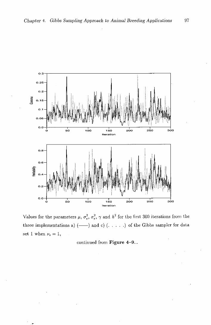
Chapter 4. Gibbs Sampling Approach to Animal Breeding Applications 97
Ca S S Ca
CD
Iteration
0.6
Ca
0.4
0.2
0.0
0 50 100 150 200 250 300
Iteration
Values for the parameters t, a, a, -y and h 2 for the first 300 iterations from the
three implementations a) ( ) and c) (.....) of the Gibbs sampler for data
set 1 when i' = 1,
continued from Figure 4-9...

Chapter 4. Gibbs Sampling Approach to Animal Breeding Applications 98
85 (Figure 4-11). There appears to be a decrease in k and M from implementation
a) to c), which is due to the fact that the gap between the iterates reduces the
serial correlations dramatically in implementations b) and c). The number of
burn-in iterations is not negligible and the higher values of k indicate the high
level of dependency in the sequence and thus slow convergence to the desired
distribution. The values of k and M were 1 and 2, respectively when v 3 = 1
for all three implementations. These results suggest that when a particular data
set experiences computational black holes it is not sensible to use v 3 < 1 at
all. Overall conclusion from applying this method is that it is not necessary to
throw away a substantial number of initial iterations (burn-in iterations) as M is
negligible. It is also not essential to discard every /cth iterate since the dependence
between successive iterates is not high which gives fast convergence. The low
dependence indicates that the convergence is achieved within first few hundred
iterations. Therefore the implementation a) seems to be the best choice compared
with others.
Absorbing state
Table 4-3 gives the marginal posterior summaries of the parameters for four data
sets when V. = e are assumed equal and taken to be 0, 0.5 and 1. As can be seen
from this table, the marginal posterior means of t and a are not affected by the
values of the prior parameters v 3 and v. However, the sire variance component,
c, and the parameters that are functions of o, 'y and h2 , appear to reach an
absorbing state depending on how low the estimate of heritability h 2 is, when
718 < 1. Consequently the marginal means get closer to zero as v 3 approaches
to zero. The examination of Table 4-3 shows that the marginal posterior means
of c, -y and h 2 are not affected by different values of v in data set 1 since the
estimate of the heritability for this particular data set is big enough, being about
0.3, to avoid the computational black hole. This is so regardless of the values of
v. However, from the marginal posterior means of these parameters in data sets
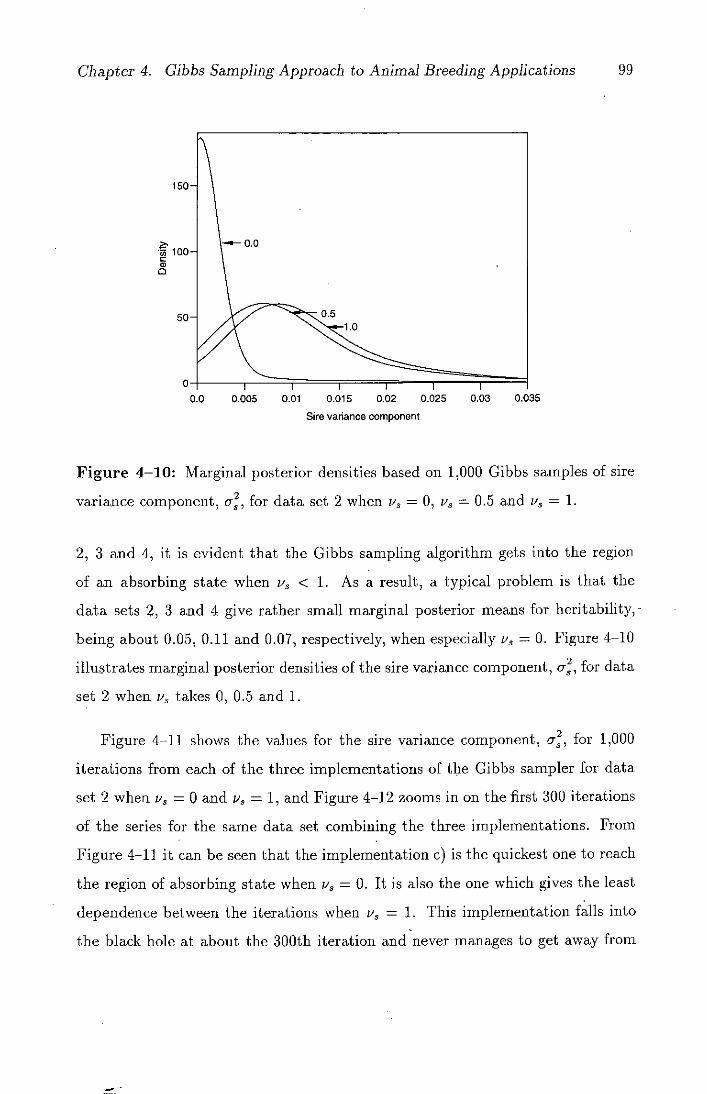
Chapter 4. Gibbs Sampling Approach to Animal Breeding Applications 99
0, C a, C
0.0 0.005 0.01 0.015 0.02 0.025 0.03 0.035
Sire variance component
Figure 4-10: Marginal posterior densities based on 1,000 Gibbs samples of sire
variance component, a, for data set 2 when V. = 0, ii. = 0.5 and v3 = 1.
2, 3 and 4, it is evident that the Gibbs sampling algorithm gets into the region
of an absorbing state when v3 < 1. As a result, a typical problem is that the
data sets 2, 3 and 4 give rather small marginal posterior means for heritability,
being about 0.05, 0.11 and 0.07, respectively, when especially P. = 0. Figure 4-10
illustrates marginal posterior densities of the sire variance component, a, for data
set 2 when v takes 0, 0.5 and 1.
Figure 4-11 shows the values for the sire variance component, 0', 2 , for 1,000
iterations from each of the three implementations of the Gibbs sampler for data
set 2 when v3 = 0 and ii. = 1, and Figure 4-12 zooms in on the first 300 iterations
of the series for the same data set combining the three implementations. From
Figure 4-11 it can be seen that the implementation c) is the quickest one to reach
the region of absorbing state when v3 = 0. It is also the one which gives the least
dependence between the iterations when v 5 = 1. This implementation falls into
the black hole at about the 300th iteration and never manages to get away from

Chapter 4. Gibbs Sampling Approach to Animal Breeding Applications
1DB]
0.07
0.00
o.0s
ft 0.04
J 0.03
0.02
0.01
0.0
Iteration
a)
0.07
0.06
ft 0-on
0.03
0.02
0.01
0.0
j it
'U 0 200 400 600 000 10
Iteration
00
b)
I Co
Iteration
C)
Figure 4-11: Values for sire variance component, a, for 1,000 iterations from
each of the three implementations of the Gibbs sampler a), b) and c) for data set
2whenv3 =0( )andv5=l(.....

Chapter 4. Gibbs Sampling Approach to Animal Breeding Applications 101
Ti,
Iteration
Figure 4-12: Values for sire variance component, a. 2 , for the first 300 iterations
from each of the three implementations of the Gibbs sampler a) ( ) b) (- - - -
-) and c) (.....) for data set 2 when v 3 = 0.
this region. Implementation a) reaches the absorbing state at about the 600th
iteration and gives the highest dependence between the iterations. Thereafter
they both cannot recover from this state of sampling until the end of series. The
implementation b) however appears to get into the absorbing region and manages
to recover occasionally. When P. increases to 1 the values of a from all three
implementations keep well away from the region of the absorbing state.
In animal breeding applications, the problem of an absorbing state is directly
related to the value of the prior degrees of freedom v 3 and can be corrected by
not using values of v 3 less than 1. Values of v 3 > 1 appear to give satisfactory
results. It can therefore be concluded that in the case of badly behaved marginal
distributions, which are associated with low heritability, it is possible to reach
an absorbing state for the values of Y. smaller than 1. This state of sampling
is influential and distorts the values of the estimated density unless ii, is large
enough.

Chapter 4. Gibbs Sampling Approach to Animal Breeding Applications 102
Table 4-4: Design of experiments simulated using different values of heritability,
h 2 , number of sires, s, and number of progeny per sire, n.
s
h2 =0.1
n S
h2 =0.3
n S
h2 =0.6
n
10 8 10 8 10 8
16 16 16
20 20 20
25 8 25 8 25 8
16 16 16
20 20 20
80 8 80 8 80 8
16 16 16
20 20 20
4.7.2 Results with 500 replicate samples
Data Sets and Designs
For this part of the analysis, 27 designs are generated with different sizes of fam-
ilies to represent situations that differ in the amount of statistical information.
Essentials of the experimental designs are given in Table 4-4. As can be seen from
this table, number of sires, .s, varies from 10 to 80, while number of progeny per
sire, i-i, ranges from 8 to 20. The smallest experimental design is the one with 10
sires and 8 progeny per sire; the largest has 80 sires and 20 progeny per sire, giv-
ing a total of 1,600 records. Data are randomly generated using parameter values
of 0.0 and 1.0 respectively for ji and a, the phenotypic variance, but different
values of heritability, h 2 . Table 4-5 shows the corresponding values for U. , c and
'y when the heritabilities range from 0.1 to 0.6. For this part of the analysis,
500 replicates are used in all simulations. In other words, for each experimental

Chapter 4. Gibbs Sampling Approach to Animal Breeding Applications 103
Table 4-5: Variance components and their functions using different starting
points
Set of starting values
Parameters 1 2 3
0.0250 0.0750 0.1500
0.9750 0.9250 0.8500
0.0256 0.0811 0.1765
0.1000 0.3000 0.6000
design 500 data sets are generated and the results of further analyses are based
on averages over these 500 replicates.
Results
The means and standard deviations of ANOVA estimates of the parameters, t, or 2
'y and h 2 , over 500 replicate samples are given in Table 4-7. Values outside the
parameter space are treated as they are. It can be seen from this table that as the
sample size and the true heritability increase, the parameter estimates, especially
o and its functions and h 2 , get closer to the true parameter values given in
Table 4-5. This can be attributed to the fact that there is a high probability of
obtaining negative estimates of or 2 when the sample size is relatively small. Table
4-6 shows the empirical and theoretical probabilities of the AN OVA estimator of
o being negative for different family sizes and heritabilities. It is also evident
from Table 4-7 that depending on the increase in the family size the standard
deviations get smaller when the heritability is kept constant.
The Gibbs Sampler is used with 1,000 iterations of 500 replicate samples, and
inferences about the parameters are based on all the values. The properties of
the posterior means of the parameters are illustrated in Table 4-8. It can be
noted that the Bayesian method overestimates the variance components and their
Chapter 4. Gibbs Sampling Approach to Animal Breeding Applications 104
Table 4-6: Empirical and theoretical (given in parentheses) probabilities of the
I ANOVA estimator of a 2 being negative when obtained from balanced one-way
model of s sires with ii progenies, under normality assumptions.
n=8
h2 =0.1
n16 n=20 n8
h2 =0.3
n16 n=20 n=5
h2 =0.6
n=16 n=20
10 0.430 0.304 0.262 0.222 0.078 0.042 0.076 0.032 0.008
(0.409) (0.305) (0.257) (0.213) (0.086) (0.057) (0.087) (0.016) (0.009)
25 0.348 0.142 0.106 0.068 0.008 0.000 0.004 0.000 0.000
(0.305) (0.162) (0.111) (0.075) (0.008) (0.003) (0.007) (0.000) (0.000)
80 0.142 0.022 0.006 0.004 0.000 0.000 0.000 0.000 0.000
(0.152) (0.029) (0.009) (0.003) (0.000) (0.000) (0.000) (0.000) (0.000)
functions 0- , 01 , -y and h2 , for designs with small family size and low heritability.
When the heritability increases for such designs the method tends to underestimate
these parameters. Thus this results in a discrepancy between marginal posterior
expectations and ANOVA estimates, the former being biased upwards and latter
being biased downward. However with an increase in the family size the estimates
appear to converge to their true parameter values and the discrepancy between
marginal posterior expectations and ANOVA estimates disappears. When the
standard deviations from both methods, ANOVA and Bayesian, are compared,
Bayesian procedure seems to give more accurate results than those of the ANOVA.
4.8 Discussion
One of the main differences between the Bayesian and maximum likelihood ap-
proaches to inference is the way in which they deal with nuisance parameters. This
is apparent from our results about, for example, 'y, thinking of p, o, a and s
as nuisance parameters. The profile likelihood function is obtained by maximising
with respect to the nuisance parameters, whereas the marginal posterior density
is obtained by a Monte Carlo numerical integration method, which is known as
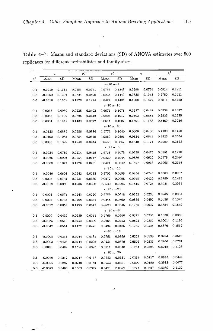
Chapter 4. Gibbs Sampling Approach to Animal Breeding Applications 105
Table 4-7: Means and standard deviations (SD) of ANOVA estimates over 500
replicates for different heritabilities and family sizes.
/2 /t2
- /t2 Mean SD Mean SD Meab SD Mean SD Mean SD
s=10 11=8
0.1 -0.0019 0.1185 0.0251 0.0741 0.9763 0.1543 0.0290 0.0791 0.0914 0.2811
0.3 -0.0062 0.1394 0.0724 0.0890 0.9235 0.1449 0.0838 0.1043 0.2780 0.3311
0.6 -0.0018 0.1559 0.1528 0.1274 0.8477 0.1435 0.1908 0.1672 0.5811 0.4350
s=10 n=16
0.1 0.0066 0.0960 0.0238 0.0403 0.9675 0.1078 0.0257 0.0428 0.0938 0.1582
0.3 0.0068 0.1192 0.0726 0.0612 0.9208 0.1017 0.0803 0.0684 0.2833 0.2235
0.6 0.0034 0.1512 0.1433 00972 0.8614 0.1002 0.1691 0.1168 0.5460 0.3286
s10 n20
0.1 -0.0123 0.0832 0.0286 0.0384 0.9775 0.1040 0.0300 0.0400 0.1108 0.1458
0.3 -0.0103 0.1084 0.0754 0.0579 0.9260 0.0896 0.0824 0.0641 0.2923 0.2064
0.6 0.0080 0.1399 0.1549 0.0944 0.8566 0.0857 0.1840 0.1174 0.5909 0.3143
s25 n8
0.1 -0.0034 0.0786 0.0214 0.0448 0.9731 0.1078 0.0239 0.0475 0.0851 0.1778
0.3 -0.0026 0.0901 0.0754 0.0547 0.9220 0.1044 0.0839 0.0620 0.2978 0.2086
0.6 -0.0069 0.1071 0.1526 0.0781 0.8474 0.0849 0.1827 0.0966 0.5966 0.2644
s=25 n=16
0.1 -0.0046 0.0601 0.0242 0.0238 0.9705 0.0698 0.0254 0.0248 0.0969 0.0937
0.3 0.0005 0.0731 0.0731 0.0380 0.9272 0.0698 0.0795 0.0420 0.2889 0.1413
0.6 -0.0019 0.0889 0.1536 0.0596 0.8530 0.0596 0.1815 0.0725 0.6021 0.2031
s25 n=20
0_1 0.0001 0.0574 0.0243 0.0220 0.9759 0.0618 0.0252 0.0230 0.0965 0.0861
0.3 0.0004 0.0737 0.0768 0.0362 0.9245 0.0599 0.0836 0.0402 0.3038 0.1340
0.6 -0.0012 0.0858 0.1493 0.0542 0.8523 0.0545 0.1760 0.0647 0.5884 0.1840
S=80 n=8
0.1 0.0000 0.0439 0.0259 0.0241 0.9769 0.0566 0.0271 0.0256 0.1030 0.0960
0.3 -0.0035 0.0510 0.0754 0.0309 0.9264 0.0553 0.0822 0.0352 0.3001 0.1196
0.6 -0.0042 0.0551 0.1472 0.0426 0.8484 0.0485 0.1745 0.0525 0.5876 0.1519
s=80 n16
0.1 -0.0005 0.0317 0.0244 0.0134 0.9751 0.0399 0.0252 0.0138 0.0974 0.0525
0.3 -0.0003 0.0403 0.0744 0.0204 0.9251 0.0379 0.0806 0.0223 0.2966 0.0761
0.6 0.0006 0.0499 0.1515 0.0325 0.8511 0.0348 0.1784 0.0394 0.6018 0.1126
s=80 n2O
0.1 -0.0010 0.0312 0.0247 0.0113 0.9753 0.0381 0.0254 0.0117 0.0985 0.0444
0.3 -0.0025 0.0397 0.0748 0.0181 0.9253 0.0361 0.0809 0.0199 0.2983 0.0677
0.6 -0.0029 0.0480 0.1503 0.0322 0.8491 0.0329 0.1774 0.0397 0.5989 0.1132

Chapter 4. Gibbs Sampling Approach to Animal Breeding Applications 106
Table 4-8: Means and standard deviations (SD) of posterior means from 500
replicate samples based on 1,000 iterations of the Gibbs sampler for different
heritabilities and family sizes.
IL
h2 Mean SD Mean SD Mean SD Mean SD Mean SD
s=10 ri=8
0.1 -0.0014 0.1192 0.0487 0.0237 0.9943 0.1512 0.0515 0.0258 0.1850 0.0846
0.3 -0.0063 0.1397 0.0886 0.0320 0.9505 0.1408 0.0974 0.0359 0.3383 0.1129
0.6 -0.0018 0.1558 0.1306 0.0387 0.8915 0.1405 0.1517 0.0441 0.5081 0.1317
s=10 n16
0.1 0.0070 0.0967 0.0401 0.0208 0.9767 0.1061 0.0424 0.0228 0.1554 0.0772
0.3 0.0077 0.1195 0.0857 0.0358 0.9350 0.1020 0.0937 0.0392 0.3283 0.1246
0.6 0.0036 0.1513 0.1343 0.0439 0.8809 0.1003 0.1548 0.0492 0.5187 0.1477
s=10 n=20
0.3 -0.0126 0.0838 0.0415 0.0241 0.9863 0.1035 0.0430 0.0251 0.1578 0.0852
0.3 -0.0103 0.1079 0.0871 0.0362 0.9378 0.0904 0.0944 0.0393 0.3311 0.1247
0.6 0.0088 0.1391 0.1405 0.0430 0.8731 0.0856 0.1632 0.0498 0.5441 0.1484
s25 n8
0.1 -0.0032 0.0788 0.0376 0.0201 0.9758 0.1028 0.0400 0.0229 0.1476 0.0782
0.3 -0.0027 0.0906 0.0822 0.0343 0.9343 0.1031 0.0907 0.0390 0.3195 0.1250
0.6 -0.0071 0.1070 0.1398 0.0424 0.8676 0.0845 0.1640 0.0490 0.5473 0.1451
s=25 n=16
0.1 -0.0045 0.0600 0.0307 0.0149 0.9744 0.0687 0.0320 0.0158 0.1211 0.0566
0.3 0.0005 0.0735 0.0794 0.0328 0.9338 0.0701 0.0863 0.0363 0.3082 0.1179
0.6 -0.0022 0.0890 0.1485 0.0405 0.8618 0.0593 0.1740 0.0481 0.5794 0.1412
s=25 n20
0.1 0.0000 0.0575 0.0297 0.0158 0.9795 0.0612 0.0308 0.0166 0.1168 0.0597
0.3 0.0001 0.0740 0.0824 0.0331 0.9299 0.0599 0.0897 0.0368 0.3203 0.1193
0.6 -0.0012 0.0848 0.1479 0.0392 0.8587 0.0547 0.1734 0.0459 0.5787 0.1344
s=80 11=8
0.1 0.0001 0.0439 0.0296 0.0146 0.9789 0.0543 0.0308 0.0158 0.1170 0.0573
0.3 -0.0034 0.0509 0.0760 0.0273 0.9320 0.0550 0.0828 0.0314 0.2995 0.1042
0.6 -0.0040 0.0552. 0.1460 0.0372 0.8543 0.0487 0.1727 0.0455 0.5787 0.1328
s=80 n16
0.1 -0.0006 0.0318 0.0252 0.0104 0.9775 0.0399 0.0260 0.0107 0.1002 0.0400
0.3 -0.0004 0.0404 0.0753 0.0200 0.9278 0.0381 0.0816 0.0219 0.2985 0.0740
0.6 0.0006 0.0504 0.1535 0.0304 0.8532 0.0349 0.1806 0.0367 0.6052 0.1049
s8O n=20
0.1 -0.0009 0.0314 0.0249 0.0095 0.9775 0.0381 0.0256 0.0100 0.0991 0.0374
0.3 -0.0024 0.0400 0.0760 0.0180 0.9272 0.0362 0.0823 0.0198 0.3014 0.0670
0.6 -0.0026 0.0480 0.1527 0.0304 0.8507 0.0328 0.1801 0.0373 0.6040 0.1063

Chapter 4. Gibbs Sampling Approach to Animal Breeding Applications 107
a Gibbs Sampler. In certain cases the two operations may produce sharply con-
trasting results. The theme is illustratedin Figures 4-7 and 4-8 for 'y and j2,
respectively. Particularly for data set 2 the marginal posterior density and profile
likelihood are quite different in shape. While the curves for the profile likelihood of
and h 2 are decreasing, this is not so for the curve of the marginal posterior den-
sity. The fact that the profile likelihood does not maximise at 0 is not in any way a
consequence of the prior distribution. However any prior which is reasonably fiat
or weak over the region of interest will result in a marginal posterior density close
to our curves skewed to the left in Figure 4-7 and 4-8. in contrast, the maximum
likelihood estimator does not correspond to any coherent set of prior beliefs, and
this must cast into serious question the use of the maximum likelihood estimator
when the log likelihood function is fax from its asymptotically quadratic shape.
4.9 Conclusion
Both the maximum likelihood and Bayesian approaches are computationally fea-
sible but there are difficulties of interpretation. The asymptotic moments of max-
imum likelihood estimates depend on the asymptotically quadratic shape of the
log likelihood function. In contrast, Bayesian methods do not rely on asymptotics
and appear to be better practical choice for handling unusually shaped likelihoods.
The difficulty of specifying a suitable prior distribution is real, but much can be
learned about the sensitivity of the analysis to the choice of prior by simply trying
out different priors. One advantage of a numerical implementation is the freedom
to do so.

Chapter 5
Investigation of Bimodality in Likelihoods
and Posterior Densities
5.1 Introduction
In animal breeding, estimates of variance components have been of great impor-
tance in the prediction of breeding values of animals and in the construction of
selection indexes. In recent years, likelihood based methods, particularly restricted
maximum likelihood (REML), has gained wide acceptance among animal breed-
ers for estimating variance components (Patterson and Thompson, 1971; Harville,
1977; Gianola and Foulley, 1990; Harville and Callanan 1990). Computational al-
gorithms like expectation-maximization (EM), Newton-Raphson, and Fisher scor-
ing, which are based on derivatives, are being used to identify the maxima of
log-likelihood functions (Groeneveld and Kovac, 1990). More recently, these nu-
merical maximization algorithms have been introduced into variance component
estimation in animal breeding (i.e. Graser et al., 1987). However, none of these
algorithms guarantees convergence to the global maximum in the presence of lo-
cal maxima. In this case, the use of likelihood-based procedures would be very
questionable, because their well-known good properties hold only if the global
maximum can be identified.
Hoeschele (1989) investigated the problem of local maxima of likelihoods and
Bayesian posterior densities when mixed linear models with two variance compo-

Chapter 5. Investigation of Bimodalityin Likelihoods and Posterior Densities 109
nents are used with unbalanced data. She concluded that the likelihood or pos-
terior density functions are always unimodal for REML and a Bayesian method
incorporating a proper inverse x2 prior but sometimes bimodal over the permis-
sible parameter space for maximum likelihood and a Bayesian method with the
improper prior density functions suggested by Gianola et al. (1990b). Groeneveld
and Kovac (1990) explored the possibilities of multiple solutions for a multivari-
ate mixed model including six covariance components by an EM and a downhill
simplex (DS) algorithm. Multiple solutions from both methods suggested the ex-
istence of local maxima, casting doubt on the merit of algorithms that do not
guarantee global maximization.
With unbalanced data and mixed linear models with two or more variance
components, iterative computing strategies are required for obtaining estimates
which maximize the likelihood function in ML and REML, or the posterior density
in Bayesian methods. If iteration converges and the converged value is within the
parameter space it is commonly assumed that at convergence the global maximum
of the likelihood or posterior density function is found. However, if the likelihood
or posterior density function has multiple maxima, convergence to a local but
not global maximum can occur, and the converged values may not be the desired
variance component estimates. This may be more likely to occur when the data
sample is small, e.g. in multiple trait estimation when the number of levels of
a random factor in the model is small relative to the number of components to
be estimated, or when variances have to be estimated within fixed classifications
because of heterogeneity of variances (Hoeschele, 1989).
In Bayesian applications with balanced data, a local maximum at zero may
occur in a one-way sire model when an improper prior density function is used
for the sire variance component, o. As a result of this, it is possible that the
marginal posterior densities of cr will be maximized at zero or near zero, creating
a bimodal posterior density function for this parameter within the permissible
parameter space.

Chapter 5. Investigation of Bimodality in Likelihoods and Posterior Densities 110
The purpose of this chapter is to investigate for a univariate balanced one-way
sire model with two variance components whether likelihood and Bayesian meth-
ods can encounter the problem of local maxima within the permissible parameter
space, and the consequences for variance component estimation when an improper
prior density function is used.
5.2 Analytical Results
5.2.1 The model
The balanced one-way sire model used in this study is
Yij = P + 3i + e (i = 1,...,s; j = 1,...,n), (5.1)
where yjj denote the phenotypic value of the jth offspring of the ith paternal
half-sib family, t represents the mean, s i is the ith random sire effect and eij
is a residual error term. The s's are distributed independently of the ejj's and
iidN(0, ), e iidN(0, (7) with Cov(s, c') = 0 for all i, i' and j, so that
E(y) = /1,
Var(y) = Ce 2 + 0 2 S
and / Cov(y,y') = c
2 . j)
5.2.2 Maximum likelihood method
If the interest is in estimating the variance components c and cr and functions of
them such as the variance ratio y = a 2 /0- 2 and the heritability h2 = 4c/(a +a)
(assuming observations are on half-sibs) rather than the si effects (sire effects or
breeding values in animal breeding), the vector of unknown parameters for model

Chapter 5. Investigation of Birnodalityin Likelihoods and Posterior Densities 111
(5.1) is 01 0,2, -y). The likelihood function for 0 1 apart from a multiplicative
constant can be given by
l(p,
S + Th3( - p12 (5.2)
1 (2)± +n±exp{_ [Sw +
1 + i
where 5b and S. are the sum of squares between and within families, respectively
and are given in Section 2.3. Let (-y) and & 2 ('y) be values of JL and a that
maximize the likelihood for given y. The profile likelihood function of 'y is then
= g({yjj}
OC (1 + ) S (S- + So
)
(0 <1/3). (5.3) 1 + 717
The profile likelihood function of 'y in (5.3) can conveniently be reparameterized
with 6 = 1 + wy and P2 = St/SW to give the following
-- P2 1(6) =g({yjj} 8;(8 6 (1 +
(1< 8 < 1 + n/3). (5.4)
The log-profile likelihood of 6 apart from additive constant is
1 /\1 ln(1(6)) = —
1 s Lin(s) + nln
+
E
)j, (5.5)
and its first derivative with respect to 6 is
31n(l(S)) I / mE\
36 F (5.6) 28 8+E
Setting (5.6) equal to zero yields S = E(m - 1) or = if j is in the
parameter space. Examination of the second derivative shows that this gives a
maximum. If E(n - 1) < 1 (i.e. (m - 1)56 < S) then there is a maximum at
6 = 1 (or7 = 0); ifE(n—l)> 1+n/3 themaxirnumis at S = l+n/3 (or = 1/3).
Therefore the likelihood function of S in (5.4) can have only one maximum which
would be anywhere between the parameter space, S E [1, 1 + n/3].

Chapter 5. Investigation of Bimodality in Likelihoods and Posterior Densities 112
5.2.3 Bayesian method
Setting the prior degrees of freedom, v, and v, to zero in (4.5) and (4.6) respec-
tively, reduces prior inverse x 2 density functions for c and 0.2 to the improper
densities
2 1 (as cc - (a > 0), (5.7)
as
and
f(c) cc - (a > 0). (5.8)
The use of improper priors, especially for o, could result in marginal posterior
densities having local maxima at zero. Bimodality is therefore inevitable.
To investigate bimodality in Bayesian methods, the marginal posterior density
function of -y, we integrate out all the other parameters, t, {sJ and c from the
joint posterior density function to give
(7)—(Us+2) (1 + fl7)_4(S_1) (5.9)
A -Y I {j}) cc Sb + + Sw + vs)
2(sn+ue+vs1)
The log of the marginal posterior density function of is given (apart from an
additive constant) by
1 1
ln(f(7 1 {yjj})) = —( v + 2) In - (s —1) ln(l + n7)
1 G i86 ++sw+ves)- —(sn+v+v—l)ln+n
The first derivative of expression (5.10) is given as follows
Oln(f(7 I yij 1(v, + 2) - ln(s —1) 1 (sn + ve v 3 -1)
87 - 2 1-1-m'y ly
nSb vS sl x
[(1 +fl7)2 +
7 r

Chapter 5. Investigation of Bimodality in Likelihoods and Posterior Densities 113
Setting (5.11) to zero and multiplying by
72(1+727)2 Sb ++sw+vese) l+n 7
yields
- [S7(1 +n7)+Vss(l+fl7)+Sb7+h/e 3 67( 1 + 727)]
x - 1)7 + (v3 + 2)(1 + n7)]
+ (sn + V 6 + v3 - 1) [vs s(1 + 777)2 + 72Sb72] = 0.
After some arrangement of (5.12) a cubic equation of the following form is obtained
a373 + a2 72 + a1 7 + ao = 0, (5.13)
where a 3 , a 2 , a 1 and a0 are given by
a3 = + V3 + 1)(S +
a2 = —n + 2v3 + 3)(S + v6s) - (s(n - 1) + V6 - 2)(Sb + nv3s)j,
a 1 = - [(V3 + 2)(S + S& + v65) - n(s(2n 1) + 2u6 - 5)v3 s 321 ,
2 a0 = (su + v6 - 3)v 3 s3 .
The cubic equation in (5.13) suggest that there may be three stationary points
but appears not to lead to any useful general result about when there is more then
one maximum. Putting v 3 = 0 makes a0 zero and gives a solution = 0 of (5.12),
so it seems more useful to look at the behaviour of the posterior density of 7 near
zero. From (5.9), it behaves like 75(8'3) (which is increasing) for v 3 > 0, but
like [1 for v3 = 0. So putting v3 = 0 produces a maximum at 7 = 0 (along with
at most one other maximum).
Chapter 5. Investigation of Bimodalityin Likelihoods and Posterior Densities 114
5.3 Numerical Results
The original four data sets generated using the model (5.1) with s i representing
sire effects (i = 1,..., 25), heritability h2 = 0.1, and progeny group size ii = 20 are
employed to investigate the possibility that the likelihood and marginal posterior
density of -Y may give multiple maxima in the parameter space. In Figure 5-1 the
profile log-likelihood functions of 'y for data sets 1, 2, 3 and 4 are plotted against
y. As can be seen from this figure the profile likelihood functions for all data
sets have a unique maximum in the permissible parameter space, [0,1/3]. The
maximum for data set 2 occurs at 0.
Figures 5-2 and 5-3 shows the log marginal posterior density functions of
for four data sets when v 5 equals 1 and 0, respectively. Figure 5-3 reveals that
when u3 = 0 only data set 1 has a Maximum with positive in addition to the
maximum at zero. However, when v = 1 it is obvious from Figure 5-2 that all
the data sets have a single maximum away from zero.
5.4 Conclusion
When using methods such as maximum likelihood or maximum posterior density
to estimate variance components, it is commonly assumed that at convergence
the likelihood or posterior density function has a single maximum in the permis-
sible parameter space. In this chapter an attempt has been made to investigate
this assumption for a balanced one-way univariate sire model with two variance
components.
Analytical results suggest that the log profile likelihood of 'y can have only one
maximum which would be anywhere in the permissible parameter space, {0, 1/31.
The log marginal posterior density function of y also has a single maximum when

Chapter 5. Investigation of Bimodalityin Likelihoods and Posterior Densities 115
V 0 0 -c
-J 0,
.3 a,
0
0-
0.0 0.05 0.1 0.15 0.2 0.25 0.3
Gamma
Figure 5-1: Plot of profile log-likelihood of 'y versus for four sets of data.
-1
0) C a, C 0) 0
—J -1
0.0 0.05 0.1 0.15 0.2 0.25 0.3
Gamma
Figure 5-2: Plot of log marginal posterior density of 'y versus for four sets of
data when u = 1.
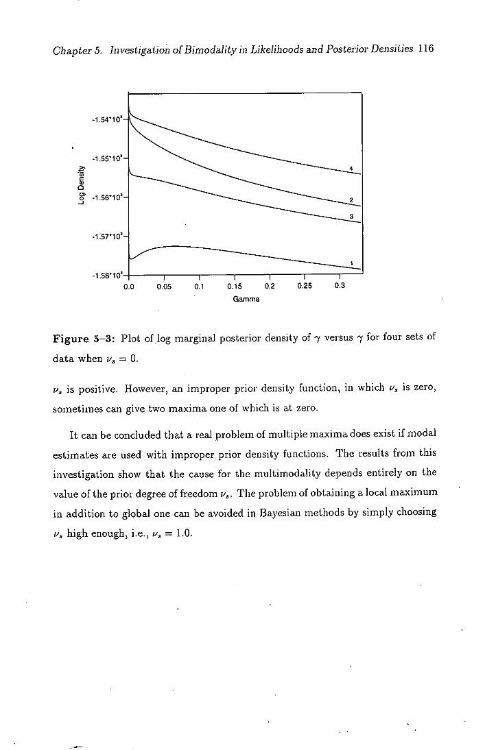
Chapter 5. Investigation of Bimodality in Likelihoods and Posterior Densities 116
U, C C, 0
8? -J
0.0 0.05 0.1 0.15 0.2 0.25 0.3
Gamma
Figure 5-3: Plot of log marginal posterior density of -y versus y for four sets of
data when v3 = 0.
1/3 is positive. However, an improper prior density function, in which v3 is zero,
sometimes can give two maxima one of which is at zero.
It can be concluded that a real problem of multiple maxima does exist if modal
estimates are used with improper prior density functions. The results from this
investigation show that the cause for the multimodality depends entirely on the
value of the prior degree of freedom v 3 . The problem of obtaining a local maximum
in addition to global one can be avoided in Bayesian methods by simply choosing
i.'5 high enough, i.e., v3 = 1.0.
Chapter 6
An Alternative Prior Specification
6.1 Introduction
A one-way sire model with equal numbers of offspring per sire is considered in
this chapter as in Chapter 4, but the purpose is to look at whether using different
prior distributions makes an important difference to posterior inferences.
A method for rejection sampling from any univariate log-concave probability
density function is proposed by Gilks and Wild (1992). Their method is adaptive
in the sense that the rejection envelope function and the squeezing function, which
form upper and lower bounds to the log-concave p;obability density function, con-
verge towards the density function as sampling proceeds. The rejection envelope
and squeezing function are piecewise exponential functions, the rejection envelope
touching the density at previously sampled points, and squeezing function forming
arcs between those points of contact (Gilks and Wild, 1992). The adaptive nature
of their technique enables samples to be drawn with few evaluations of the density
function and it is therefore intended for situations where evaluation of the density
is computationally expensive, in particular for applications of Gibbs sampling to
Bayesian models with non-conjugacy. Applications of adaptive rejection sampling
currently include generalized linear and proportional hazards models (Dellaportas
and Smith, 1993).
Basic to the implementation of the Gibbs sampler is the ability to sample
from the full conditional distribution of each parameter conditioning on all the
117
Chapter 6. An Alternative Prior Specification 118
remaining parameters and the data. Gibbs sampling has been applied in many
areas including variance components, errors-in-variables, missing data and growth
curve problems. In essence these applications have focused on situations in which
there is conjugacy between likelihoods and priors, for which the sampling involved
in Gibbs sampling is straightforward.
Without conjugacy sampling could be difficult and very expensive computa-
tionally, particularly when there are many observations {yj}. Moreover, for each
parameter, Gibbs sampling requires only one point to be sampled from the cor-
responding full conditional distribution: at the next iteration the full conditional
will be different (through conditioning on different. values of the remaining param-
eters). One should therefore seek a sampling method which minimizes the number
of evaluations.
However, other classes of problems exist (e.g., non-linear regression) where the
posterior distribution is lacking conjugacy in at least one of the full conditionals.
Recently, several methods have been proposed for dealing with non-conjugate
conditionals via importance sampling or acceptance/rejection approaches. Zeger
and Karim (1991) present rejection sampling from a normal envelope centred at the
mode of the sampling density in an application of the Gibbs sampling procedure to
the posterior expectation of generalised linear models with random effects. Gilks
and Wild (1992) show that adaptive rejection sampling is well suited to handling
non-conjugacy in applications of Gibbs sampling.
The application of Gibbs sampling using a balanced one-way univariate sire
model in animal breeding is carried out for fully conditionally conjugate Bayesian
models with parameters i, {.s}, o 2 and o- in Chapter 4. Prior specification
employed in that chapter will be referred to from now on as prior specification
I. Reparameterization from (o, o) to (-y, c) with 'y equal to o/c can cause
non-conjugacy and consequently computational difficulties. This reparameterized
prior specification will be called prior specification II throughout this thesis. The
Chapter 6. An Alternative Prior Specification 119
objective of this chapter is to demonstrate how the Gibbs sampling procedure,
making use of an adaptive rejection sampling algorithm, deals with non-conjugacy
due to reparameterization for a balanced one-way univariate classification with
random sire effects and to compare the results from using the reparameterized
prior specification with those for the prior specification of Chapter 4 obtained
from fully conjugate conditional posterior density functions.
6.2 An Alternative Bayesian Model
6.2.1 Prior distributions
Prior distributions of IL and u, 2 . An alternative prior specification might have 1L
uniform and o- 2 inverse-x 2 as in prior specification I, but with a independent of
7
Prior distributions of the s. The normal distributions assigned to the s i 's as
prior probability distributions can be given by
S
(2) - 9 5 ( 1 sfl. (6.1) f({s} y,a) exp 27a i=1 I
Prior distribution of 7. Prior information about the ratio of two variances a
and o, , of a certain trait in a certain livestock is required. Then, in some cases,
it may be natural that a prior distribution of 7 is considered as some unimodal or
uniform distribution within a certain range. Consequently the prior distribution
of 7 might be considered as beta distribution with a range [a, b] (in this case the
range must be within [0, 1/3] interval because of the natural restriction imposed
on 7 (see Section 2.4.1), but generally it may be only finite), and this distribution
is called a generalized beta distribution. In the conventional consideration, the
generalized beta distribution can be used as a prior distribution of any other
genetic parameter defined in a finite range, say genetic correlation coefficient and

Chapter 6. An Alternative Prior Specification 120
heritability as well as the ratio of variances. The generalized beta density (see
Appendix A for detailed description of this distribution) for the prior distribution
of 'y can be written as follows
a—i /3—i f(7a,/3)(7—a) (b-7) , a7<b,
where the interval [a, b] corresponds to the proper range of 'y, [0, 1/3], then
i i f( a) a— (1-37) /3- 0<7<1/3. (6.2)
The truncated F distribution is also another possibility for the prior distribution
of .
Determination of the prior parameters, a and /3
After specifying a Beta form for the prior distribution of , it is useful for compar-
ison to determine values of the parameters a and 0 of this distribution for which
the two prior specifications match in some sense. Recall that in prior specification
I 2
Wa = x (v 3 )
as
and 2
We = x (v4 ; cr
then joint density is taken to be the product of the corresponding densities if
30.2 cc o 2 and zero otherwise. Hence
2 2 2/ \ 2/ 7 = °s/°e = (vss s /Ws)/(ves e /We)
- s (we\ / (W
- s \VeP v 3
= o<J<(3) i se

Chapter 6. An Alternative Prior Specification 121
To find the quartiles of ,y for prior specification I and hence a matching Beta dis-
tribution, consider the distribution of J, which is F(ue , u3 ) truncated at.s/(3s).
If G(f; lie, u3 ) denotes the distribution function of F(ue , v5 ) then f has lower and
upper quartiles fL, fu which are solutions of
2 I
G(fL; lie, u5 ) = 0.25 c'9 2
ye , us) US
G(fu; lie, u8 ) = 0.75 C V, VS)
and 'y has quartiles s/sfL, s!/sfu. The corresponding quartiles of 37 are then
equated to those of a B(a, 0) distribution.
Thus if XL and zu denote the lower and upper quartiles of the distribution
B(a, 0), we equate XL and xu to (38 2 /8 2 )fi. and ( 3S 2 /S 2 )fu respectively, and
solve the following equations for a and .# in prior specification II
1 (XL 0.25 = 0 (6.3)
B(a,/3 ) Jo
and
1 fXU
J —0.75 = 0. (6.4)
B(a, 0) 0 - --
Example: Let s = 0.025 and s = 0.975 then the distribution of 7, F(ue, u5 ),
is truncated at .s/(3s) = 13 when u5 = v. = 1.0 in prior specification I. This 61 11
gives G(13; 1, 1) = 0.8278. Lower and upper quartiles fL, fu of the distribution
of 7 are solutions of
G(fL; v,, u 5 ) = 0.25 G(13; 1,1) = 0.25 x 0.8278 = 0.2065
G(fu; v, u 5 ) = 0.75 G(13; 1,1) = 0.75 >< 0.8278 = 0.6209 1
respectively. Solutions to these equations are found as fL = 0.1136 and fu =
2.1777. The corresponding quartiles of 37 in prior specification II are equated to
those of a Beta distribution giving the following quartiles
XL = ( 3s/s)fL = 0.0731 x 0.1136 = 0.0087

Chapter 6. An Alternative Prior Specification 122
, xu = (3s 2, S2e)fU = 0.0731 x 0.2.1777 = 0.1675
Finally, the quartiles XL, xu are substituted in equations (6.3) and (6.4)
and
1 0.0087
B(a,(3) Jo
1 0.1675
B(a,fl) Jo
- —0.25 = 0
1(1 - 7)1 —0.75 = 0.
and these equations are solved for a and 0 to obtain 0.4038 and 3.0678, respec-
tively, for this particular example.
Prior distribution of o. The prior distribution of c can be obtained from
the prior distributions of a 2 and 'y given in (4.5) and (6.2), respectively, since
o- is given by -ya. The determinant of the Jacobian of the transformation from
( _Y, a2) to (o,a) is f'. The joint probability density function of or and 2' is
then proportional to
a, (3, Ve, s) ( a 2 )_ 2)72+va_2)(1 - 37)' exp ( 1 7Ve3 '2
The prior probability density function of or can then be given by
I1/3
1 f(a a, 0, Ve, s) c3 )_ v2 ) 75(2a+ve_2)(1 - 37)1 (2
0
H ves) (6.5) >< exp
Evaluation of expression (6.5) requires numerical methods.
Prior distribution of h 2 . Since h2 = 417
, the prior probability density function
of it 2 is proportional to
f(h2 I a,(3) (_h \al
- h2) [i - (_it2
(4— h22
oc (h 2 ) 1 (4 - h2)(1 - h 2)', 0 < h2 1. (6.6)

Chapter 6. An Alternative Prior Specification 123
6.2.2 Likelihood function
The likelihood function for it {s}, C is given by
2 2 1 1 f({yij} 7,Ce) (c e ) expj — -- —p - si)] }. (6.7)
i=1 j=1
6.2.3 Joint posterior distribution
Using the likelihood in expression (6.7) in conjunction with the prior distributions
for the prior specification II, for p, {s}, a and 7 given in (4.3), (6.1), (4.6) and
(6.2), respectively, the joint posterior distribution is proportional to the product
of the densities corresponding to these distributions
f(p,j8 i 1,
7, C2 1
yjj) exp i
(yjj - p - s) 2 + r
2a I Li=1 j=1 7 11
( 2 ) (8(Th+1)++2) (-2o,2
2"exp ves e )
X 72(32a+2)(1 - 37 1) 0 . ( 6.8)
6.2.4 Full conditional distributions of i, Si, U and -y
Conditional posterior distribution of p. The full conditional posterior distribution
of p given {s}, and a 2 is not affected by the prior specification II. It is therefore
the same as (4.22),
= N ( - , j. (6.9)
ns)
Conditional posterior distribution of the s. The posterior probability density
function (6.8) is proportional in the si to
1 [ s(i + n) - 2nE1 p) = l -Yore C j

Chapter 6. An Alternative Prior Specification 124
or ( i (1+n\ r3
exp 7C ) L4 2n
- 77_ - it)l
L=i 1+n7
thus the full conditional distribution of si given p 'y and c 2 is
[s p,7,a,{yij}] = N (n7(i - ) \
(6.10) \ l+n ' l+n7)
independently of s. (Ii i). This is also not affected by the prior specification II
and therefore the same as (4.23).
Conditional posterior distribution of 01, 2 . The posterior probability density
function (6.8) is proportional in a to
()8(Th+i)6+2) exp {_L [tt - p - ) 2 + + ves] }, Ore
thus the full conditional distribution of or given p, s i and -y is
[c S 72 2
= x2 (s(n + 1) + v, (yjj - p - s) 2 + '
5 +e) i=1 j=1 7
Conditional posterior distribution of . The full conditional distribution of 7
given p, {s} and o 2 is
15i}, 0,2 , yijl 72(S2+2)(1 - 3t1 exp {
_ E s/a Y, {s (6.12)
2 j
The full conditional distributions of p, the s i and 0,2 given respectively in
(6.9), (6.10) and (6.11) are conditionally conjugate. However the full conditional
distribution of 'y in (6.12) is frôma 3-parameter family with probability density
function proportional to
(- 2 ,y) 7"(1 - 37) b exp
lc
and does not simplify. This is not a well-known family, therefore it is not im-
mediately clear how to sample from it and sampling 7 could be time consuming.

Chapter 6. An Alternative Prior Specification 125
Whereas the application of Gibbs sampling is straightforward for fully conjugate
Bayesian models, non-conjugacy in 'y can cause computational difficulties. Adap-
tive rejection sampling is well suited to handling non-conjugacy in application of
Gibbs sampling, as it requires neither the mode of the sampling density nor a
rejection envelope that corresponds to a standard density (Gilks and Wild, 1992).
The graphical representation of the Bayesian random effect model for prior
specification I with three sire families is discussed in Section 4.4. The directed
acyclic and conditional independence graphs for prior specification II with three
families giving the observed data D1 , D2 and D3 are shown in Figures 6-1 and
6-2, respectively. The full conditional distributions corresponding to the graph of
Figure 6-2 are already given in this section.
6.3 Adaptive Rejection Sampling From Log - con-
cave Density Functions
An important family of univariate density functions is the family of log-concave
density functions. This family includes many common probability density func-
tions see, for example, Gilks and Wild (1992). Firstly a formal definition of what
is meant by log-concavity will be given. This is then followed by a description of a
specific rejection sampling method for dealing with log-concave density functions.
Log-concavity. Assume that the density function f(x) is continuous and differ-
entiable on an open convex set D in R (where D denotes the domain of f(x)).
Then f(x) is called log-concave with respect to x if h(x)_-=.lnf(x) is. concave.
everywhere in D, i.e., h'(x) = dh(x)/dx decreases monotonically with increasing
x in D. This definition of log-concavity admits both straight line segments on the
log density h(x) and discontinuities in h'(x).
Non-adaptive rejection sampling (Rejection ampling). The log-concavity of a
density function enables one to use specifically designed algorithms for the genera-

Chapter 6. An Alternative Prior Specification 126
Figure 6-1: Directed acyclic graph of the Bayesian random effects model for
prior specification II with three families s 1 , 3 2 and 53 giving the observed data D 1 ,
D2 and JJ.
Figure 6-2: Conditional independence (undirected) graph for the Bayesian ran-
dom effects model for prior specification II.

Chapter 6. An Alternative Prior Specification 127
tion of random variates. Rejection sampling is a method for drawing independent
samples from a distribution (proportional to) f(x) and does not involve evalua-
tion of the integration constant ID f(x)dx. This is very convenient for sampling
from full conditional distributions, which are typically known up to a constant of
proportionality. However, rejection sampling is only useful if it is more efficient
or convenient to sample from the envelope function of f(x) than from the density
f(x) itself. In practice, finding a suitable envelope function can be difficult and
often involves locating the supremum of f(x) in D by using a standard optimiza-
tion technique (Gilks and Wild, 1992), which is a time-consuming maximization
step.
Adaptive rejection sampling. For Gibbs sampling, usually only one sample is
required from each density, although sampling from many thousands of different
densities may be required. Moreover, when estimating a model involving non-
conjugacy, evaluations of f(x) may be computationally expensive. In these cir-
cumstances rejection sampling may be very inefficient, since it may involve many
thousands of optimizations, each involving several evaluations of f(x). Recently,
Gilks and Wild (1992) have proposed an adaptive rejection sampling method of
sampling from any log-concave univariate probability density function, which has
the important advantage of avoiding such optimization. Their suggested algorithm
is based on the fact that any concave function can be bounded by piecewise linear
upper (rejection envelope) and lower bounds (squeezing function), constructed by
using tangents at, and chords between, evaluated points on the function over its
domain. Dellaportas and Smith (1993) applied this result to generalized linear
and proportional hazards models with-canonical links. The detailed-procedure is__.
as follows.
Assume that we need to generate random variates from the univariate prob-
ability density function f(x) exp h(x), say. Suppose h(x) and h'(x) have been
evaluated at k ordered points in D: x1 ... < xk. Assume also that the
mode of h(x) is between x 1 and xk, and that h(x) is continuous and differentiable

Chapter 6. An Alternative Prior Specification 128
X - x 2 x3
Figure 6-3: A concave log-density h(x) for adaptive rejection sampling showing
upper and lower hulls based on three starting values (x 1 ,x 2 ,x3) : ( ), h(x); (-
- - - )' u 3(x); (.......), l(x).
on a real interval (a, b), where a and b can be —oo or oo , and that the second
derivative is non-positive throughout (a, b). Let 7), = {x : i = 1,. . . , k} and
define the rejection envelope and the squeezing function on T,,, as expuk(x) and
exp lk(x), respectively, where uk(x) is a piecewise linear upper hull formed from
the tangents to h(x) at the abscissae in Tk
uk(x) = h(x) +(x — x)h'(x) (j = 1,.. .,k)
and lk(x) is a piecewise linear lower hull formed from the chords between adjacent
abscissae in 7),
L(x) = ( x +i - x)h(x) + (x — xa)h(xj+i) k - 1)
xj+1 — Xi
Finally, we define
exp uk(x) Sk(X) = ID exp uk(x
F)dx
Figure 6-3 illustrates a log-concave density showing upper and lower hulls based
on three starting points. In this figure the continuous curve exemplifies a concave
h(x) in a domain D, the upper broken curve is uk(x) and the lower broken curve
is lk(x).

Chapter 6. An Alternative Prior Specification 129
Thus the rejection envelope and the squeezing function are pairwise exponential
functions. The concavity of h(x) ensures that lk(X) < h(x) < Uk(X) for all x in D.
To sample n points independently from f(x) by adaptive rejection sampling,
proceed the following algorithm.
Initialization step
Initialise the abscissae in Tk. If D is unbounded on the left then choose x 1
such that h'(x i ) > 0. If D is unbounded on the right then choose xk such that
ri h (Xk) < 0. Then calculate the functions uk(x), 5k(X) and lk(X).
Sampling step
Repeat until desired number of points have been sampled.
Sample a value x from 3k(x) and a value u independently from the uniform
(0,1) distribution. Perform the following squeezing test:
If u <— eXPIlk(X*) - Uk(X)} then
Accept x
Else evaluate h(x*) and h'(x*) and perform the following rejection test:
If u < exp{h(x*) - flk(X)} then
Accept x
Else
Reject x"
End if
Updating step
Include x' in Tk to form Tk+1, increment Iv, relabel the members of Tk in
ascending order, construct the functions nk+1(x), sk+1(x) and 1k+1 (X) on the basis
Of Tk+l.

Chapter 6. An Alternative Prior Specification 130
End if
End Repeat if n points have not yet accepted.
The adaptive rejection sampling algorithm has two important advantages com-
pared with other existing general purpose methods for generating independent
observations from a probability density function.
Firstly, unlike the other existing methods for generating random variates from
log-concave density functions, such as the rejection sampling or the ratio of uni-
forms methodrmoves the need to locate the supremum of f(x) in D. Except for
some well-known densities, locating the mode necessitates the use of numerical op-
timization routines, which require an average of seven or eight function evaluations
for the kinds of density arising from generalized linear models and proportional
hazards models (Dellaportas and Smith, 1993). Gilks and Wild (1992) reported
an average of three function evaluations per iteration to obtain one sample of size
1 using the adaptive rejection sampling algorithm.
Secondly, it is adaptive in the sense that after each rejection, the probability of
needing to evaluate f(x) further is reduced by updating the envelope and squeezing
functions to incorporate the most recently acquired information about f(x) (Gilks
and Wild, 1992), because, with the addition of more points, the density function
is closer to the upper and lower functions used to squeeze it.
6.3.1 Adaptive rejection sampling and Gibbs sampling
Gibbs sampling
As was stated in Chapter 4, Gibbs sampling requires specification of the full
conditional distribution for each parameter. The full conditional distributions
of It, the s, or and are given in (6.9), (6.10), (6.11) and (6.12), respectively.
Often the likelihood and prior forms specified in Bayesian analysis lead to the

Chapter 6. An Alternative Prior Specification 131
distributions which are of a familiar form, such as the normals for IL and {s} given
in expressions (6.9) and (6.10), respectively, or the inverse x2 for U2 in (6.11). In
these cases, standard algorithms are available to generate random variates.
Proportionality in (6.12) implies that the full conditional density for 'y differs
from the right-hand side of expression only by a multiplicative term which does
not depend on 'y. Unless there is conjugacy, the full conditional will not corre-
spond to a common distribution and it may not be possible to derive a closed
form for the proportionality constant in expression (6.12). Moreover, since it is
the product of several terms, expression (6.12) will be computationally expensive
to evaluate repeatedly using standard algorithms. In this case, random variate
generating methods such as the 'inversion method', the 'rejection 'method', the
'ratio of uniforms method', the 'adaptive rejection method' or the 'adaptive rejec-
tion metropolis method' applicable to wide ranges of distributions, can be used.
However, depending on the nature of the distribution family, an efficient choice of
a method generally requires mathematical insight on the part of the designer of
the sampling scheme, e.g. exploiting a property of log-concavity, or knowledge of
certain density characteristics such as the supremum of the density or the explicit
form of the inverse of the cumulative density function. In addition, owing to their
'universality', these methods do not compete in efficiency with special purpose
algorithms designed for the generation of random variates from popular densities.
It is therefore evident that special care must be taken in both the choice and the
design of such methods in the application of Gibbs sampling.
Log-concavity
The application of the adaptive rejection sampling method described earlier re-
quires the log-concavity of the full conditional distributions with respect to pa-
rameter of interest. When this is not so, the log-density may be concave with
respect to a suitably transformed parameter (taking account of the Jacobian).

Chapter 6. An Alternative Prior Specification 132
Therefore each of the terms in expression (6.12) should be checked whether they
are concave on the logarithfnic scale with respect to 'y so that adaptive rejection
sampling can be used. The log density can be given as follows
h(1) = ln{7 P,i,,YijI
= —(s-2a+2)in7+(fl—l)ln(l-37 (6.13)) 2
For adaptive rejection sampling of y it is required that equation (6.13) is contin-
uous, differentiable and log-concave with respect to y. The terms in this expression
are not concave with respect to when (s - 2a + 2) > 0 and 0 < 3 < 1, and
consequently h(7) is not concave.
The log transformation of 'y, 5 = in , can be used to obtain log-concavity for
this density. The Jacobian of this transformation is e 6 . The transformed log
density is given except for an additive constant by
h(S) = ln[S 1L4, Si, 0, yij]
1 1 >T7....1 .s
= —(s-2a)S+(/3—l)ln(l-3e5)— 2 e , —cc<S<ln(1/3).
(6.14)
The second derivative of expression (6.14) with respect to S is
82 h(S) - 13(/3 - 1)e 8 - 1 Si2 e < 0. (6.15) 852 - 2(1-3e 8 ) 2 2 a
Thus condition (6.15) guarantees log-concavity when 0 > 1. A caution must
therefore be taken when using h(S) in (6.14) since it is sensitive to the values of
0. Especially, when 0 < 1 a prior probability density function tends to cc as
tends to 1/3, which is not sensible. In this chapter, numerical examples will ke
given for the cases where the value of /3 is greater than unity.

Chapter 6. An Alternative Prior Specification 133
In cases where the full posterior conditional density is not log-concave, Gilks
et al. (1993) generalised adaptive rejection sampling to include a Metropolis al-
gorithm step. This case will not be considered further in this thesis.
6.4 Illustrative Examples and Results
Adaptive rejection sampling has been applied to a Gibbs sampling analysis, of four
data sets generated using one-way sire model when V. = = 1, s 2 = 0.025 and
= 0.975 giving a = 0.4038 and 0 = 3.0678. Recall from section 6.2.1 that
the values of a and 0 are determined by the values of v 3 , lie, s and .s. Table
6-1 illustrates the values of a and /3 for changing values of heritability, h 2 when
V 8 =V, = 1 and s 2 + 82 = 1. It can be seen from this table that as h 2 increases /3
decreases, and when h 2 is more than about 0.3, 0 becomes smaller than one. In
this section examples will be illustrated for the case in which h 2 = 0.1, 82 S
= 0.025
and s 2 e = 0.975. The output from the Gibbs sampling procedure is used to present
inference summaries for the parameters of the sire model. Moreover the results
of this section using the prior specification II will be compared with those of the
prior specification I.
Table 6-1: Values of a and 0 corresponding to different values of h 2 for
V 8 _V ' = 1.
h 2 s 2 8 2 a /3
0.1 0.025 0.975 0.4038 3.0678
0.3 0.075 0.925 0.3630 0.8400
0.5 0.125 0.875 0.2700 0.2841
Recall the form of the joint posterior density for the model parameters ji,
and cr, given by the density function (6.8). By virtue of the earlier discussion,

Chapter 6. An Alternative Prior Specification 134
Gibbs sampling is carried out using the log transformation of 'y, S = In-Y; the
exponential of expression (6.14) gives the full conditional posterior density function
of 8 up to proportionality. At each iteration of Gibbs sampling algorithm, adaptive
rejection sampling from this full conditional posterior density requires at least two
points which can be used as initial points for the construction of upper and lower
bounds. Since the parameter space for 8 is unbounded on the left, one of the
initial points, 61 is chosen to satisfy the condition h'(8 1 ) > 0. After initializing the
Gibbs sampling procedure with two points, replications of the iterative algorithm
proceed independently and the 15th and 85th centiles of the sampling density
sk(x) from the previous iteration of Gibbs sampling were used as starting values
for adaptive rejection sampling. In cases where the two initial points did not lie
on either side of the mode of the conditional posterior density, additional points
were supplied.
An assessment of convergence of the process was made by monitoring a number
of summary statistics based on every 10 iterations for each parameter. In this
section, 1,000 iterations of the Gibbs sampling procedure were performed, by
which time convergence had clearly occured and direct numerical and graphical
comparisons of marginal posterior densities with those from the prior specification
I were made. Therefore the resulting marginal posterior summaries in Table 6-2
were based on 1,000 iterations.
The results in Table 6-2 seem to agree with those in Table 4-3 when v8 = v, =
1.0 for 1,000 iterations. Marginal posterior densities for the model parameters
01 2 , o, 'y and h 2 constructed from 1,000 samples for both prior specifications are
shown in Figures 6-4 to 6-8, respectively. A visual inspection of the marginal
posterior densities in these figures provides more insight into the comparison of
the two prior specifications. The posterior distributions look very similar when t
and o 2 are considered, but slightly less so when o, -y or are examined.
As the basis for constructing hulls to deliver a variate value from the full

Chapter 6. An Alternative Prior Specification 135
Table 6-2: Marginal posterior means and standard deviations of parameters for
four data sets using prior specification II based on 1,000 iterations of the Gibbs
sampler for a sire model with 25 families of size 20.
92 2
-y
Mean SD Mean SD Mean SD Mean SD Mean SD
DATA SET 1
-0.0261 0.0731 0.0887 0.0388 1.0632 0.0686 0.0837 0.0362 0.3047 0.1209
DATA SET 2
0.0716 0.0489 0.0119 0.0099 0.9836 0.0625 0.0121 0.0100 0.0472 0.0383
- DATA SET 3
0.0407 0.0558 0.0288 0.0219 1.0200 0.0660 0.0284 0.0217 0.1087 0.0797
DATA SET 4
-0.0311 0.0500 0.0182 0.0146 0.9677 0.0620 0.0188 0.0151 0.0730 0.0568
conditional density function of 5, an average of three evaluations of h(S) were
required at each iteration by the adaptive rejection sampling.
6.5 Conclusion
The adaptive rejection sampling algorithm of Gilks and Wild (1992) can be used -
for efficiently sampling from complex univariate densities. In particular, it is useful
for applications of Gibbs sampling to the analysis of Bayesian models which involve
non-conjugacy.
The results of this chapter have clearly demonstrat(4that in animal breeding
applications the use of different prior distributions leads to the same marginal pos-
terior inferences on each parameter when a balanced univariate one-way sire model
with equal number of offspring per sire is considered for both prior specifications.
This shows that the marginal posterior density is robust to changes in the prior
specifications. In particular, no appreciable changes in the marginal posterior dis-
tribution are observed if the parameters of prior specification I is reparameterized
from (o, o- ) to (-y, c). The posterior expectations are very similar for different
prior 'specification.
Chapter 6. An Alternative Prior Specification 136
8-
7-
6- / 7
- 2 4 -
5- --
3
4- 1 • /
3-
2- 1'
0 - -- - -- I I -
-0.3 -0.2 -0.1 0.0 0.1 0.2 0.3
Mean
Figure 6-4: Marginal posterior density of IL from both prior specification for
four sets of data, ( ), prior specification I; (-----), prior specification II.
3' 0) C 0) C
(0 C (0 C
0.0 0.05 0.1 0.15 0.2
Sire variance component
Figure 6-5: Prior (.....) and marginal posterior densities of c 2 from both
prior specification for four sets of data, ( ), prior specification I; (-----), prior
specification II.

Chapter 6. An Alternative Prior Specification 137
0, C 0 C
0.0 02 OA 0.6 0.8 1.0 12 1.4 1.6
Residual variance component
Figure 6-6: Prior (.....) and marginal posterior densities of o from both
prior specification for four sets of data, ( ), prior specification I; (-----), prior
specification II.
0, C 0 0
0.0 0.05 0.1 0.15 0.2
Gamma
Figure 6-7: Prior (.....) and marginal posterior densities of ' from both
prior specification for four sets of data, ( ), prior specification I; (-----), prior
specification II.

11
Chapter 6. An Alternative Prior Specification 138
ha 0 C a) C
0.0 0.1 0.2 0.3 0.4 0.5 0.6 0.7
Heritability
Figure 6-8: Prior (.....) and marginal posterior densities of h 2 from both
prior specification for four sets of data,
specification II.
), prior specification I (-----), prior
Although conceptually straightforward, care must be taken in the implementa-
tion of adaptive rejection sampling when the log density is sensitive to the values
of parameter (e.g. values of 0 less than 1 are not sensible).

Chapter 7
Theory of Selection Indices For a Single
Trait
7.1 Introduction
The selection index employed in animal breeding refers usually to a linear com-
bination of observations that is used to compute, for each individual available for
choice, a criterion (index value) for selection. The mathematical description of
this linear function is called the selection index, I, and a numerical value actually
computed by an index from the observations on a particular individual, the selec-
tion criterion. The selection of animals for breeding involves the choice of a subset
of the individuals available on the basis of a number of measurements on each of
them. These measurements may be made on the candidates themselves and their
relatives or, as in the case of the selection of bulls in order to improve the yield or
quality of milk, on their offspring or other relatives.
The variation between individuals in the traits measured is partly the result
of differences in genotype as well as the environment, and it is the genotype of
an individual which determines its value for breeding. The breeding value of
an animal is defined by a function - usually taken to be linear - of the genetic
characteristics corresponding to the traits measured, this function being intended
to reflect their economic value.
Selection indices can be used for several purposes, e.g.,
[gI]

Chapter 7. Theory of Selection Indices For a Single Trait 140
Selection on a single trait using information on an individual and its collat-
eral relatives.
Selection on two or more traits using records on the individual alone.
Selection on two or more traits using records on the individual and its rela-
tives.
Selection of line-crosses using data in addition to that on the specific cross.
The selection index procedure is strictly justified only for the case in which the
information available on each candidate for selection is the same. More precisely,
the records and underlying genetic value available on each individual are a random
sample from some known population. In animal breeding this is seldom true
Essentially the selection index developed and elaborated by the above men-
tioned authors is a linearly-weighted function of observations on an individual
and/or its relatives for one or more traits, in order to select those individuals
expected to have the highest breeding value and thus, the best progeny. Their
theory is based on the assumption that the form of the distribution and the pop-
ulation parameters such as heritabilities and genetic and phenotypic correlations
are known exactly. In practice, however, only finite samples from distributions
indexed by those parameters are available in order to construct an index, and
use of estimates based on the sample data rather than the true parameters will
therefore lead to t less efficient index than one computed from the parameters
themselves. Several studies have been undertaken of the effects of sampling vari-
ation in the parameter estimates and the loss in efficiency in terms of the size of
the sample used for estimation by Williams (1962a, b), Harris (1964), and Sales
and Hill (1976, 1977).
Sales and Hill (1976) considered the effects of errors in estimates of parameters
on the response from selection for one trait using an index combining individual

Chapter 7. Theory of Selection Indices For a Single Trait 141
and full- and/or half-sib family records. They made some comparisons between
the theoretically optimum progress, the predicted progress and the actual progress
when the index computed from parameter estimates was used in the population. In
a model where only one of two traits was assumed to be of economic importance,
but the second trait might he correlated with it, Sales and Hill (1977) showed
that inclusion of the second trait (i.e. use of the estimated rather than the base
index) was likely to be worthwhile only when reliable estimates of parameters are
available. Further, they showed that, if the second trait really contributed nothing
useful, the greater the benefit predicted from its inclusion, the greater the real loss
in efficiency if it were included.
In a simply designed experiment with non-overlapping generations, response to
selection may be estimated using least-squares procedures as the phenotypic mean
of the offspring of selected parents. Sorensen and Kennedy (1984) discussed and
compared properties of the least-squares estimators of selection response and an
alternative estimator based on mixed model procedures. Sorensen and Kennedy
(1986) extended their earlier results through computer simulation. Both stud-
ies concluded that mixed model methods can offer advantages over least-squares
techniques.
An alternative way of estimating response to selection is to use a mixed model
approach. Henderson (1975) has shown that when selection involves culling on
the basis of past performance then under certain conditions, the mixed model
equations without selection lead to best linear unbiased estimators (BLUE) of
estimable functions of fixed effects and best linear unbiased predictors (BLUP) of
the random effects of the model. In fact, these estimators and predictors are the
same ones that would be obtained if it is assumed that selection has not occured.
These conditions are:
i) the model is correct one;
ii) selection is on a linear function of the records,

Chapter 7. Theory of Selection Indices For a Single Trait 142
the ratios of the variances of the random effects prior to selection are known
(e.g. heritability),
the random effects before selection are multivariate normally distributed,
and
selection is invariant to the fixed effects in the model.
Many selection programmes in farm animals are based on BLUP using mixed
model equations in order to predict breeding values and rank animals for selec-
tion. Section 2.4.5 describes the prediction of breeding values for a single trait
sire model. The condition Hi) of the BLUP is in common with selection index.
Therefore, the predictions of the breeding values and genetic means, which are
computed as the average of the BLUP of the genetic values of the appropriate
individuals, depend on the variance ratios such as heritability. In turn, the esti-
mates of genetic change which is expressed as the regression of the mean predicted
additive genetic value on time or on appropriate cumulative selection differential
(Blair and Pollak, 1984), depends on the ratios of the variances of the random
effects used as prior values for solving mixed model equations.
So far it has been assumed that the heritability or the ratios of the variances of
the random effects in the base population is known and used in the mixed model
equations to compute response to selection. What can be done if the initial heri-
tability is not known? There are at least two approaches to follow. One is to use
a prior value based on information from the literature. Sorensen and Kennedy
(1984) tested the use of a wrong prior value in their simulation to compute re-
sponse using mixed model equations. Henderson (1975) showed that predicted
breeding values are biased when the prior value is regarded as constant. The
other approach is to obtain an estimate from the data. One can obtain an esti-
mate of the base population heritability using the REML estimate or some other
estimate. The estimate can then be used in the mixed model equations to compute

Chapter]. Theory of Selection Indices For a Single Trait 143
the response. Some properties of the BLTJP estimator of response computed by
replacing unknown variances by likelihood estimates were examined by Sorensen to
and Kennedy (1986). In view of these approaches, it is reasonableexpect that
the statistical properties of the BLUP estimator of response will depend on the
method with which the prior heritability is estimated.
One should notice that in the second approach taken above, the prior value
is not a constant but a random variable. If the estimator is unbiased, the ex-
pected estimate of response should equal the true response, assuming the model
is correct (condition i) of BLUP). No other properties of BLUP are known and
these would be difficult to derive because of the nonlinearity of the predictor. In
selected populations, frequentist properties of predictors of breeding value based
on estimated variances have not been derived analytically using conventional sta-
tistical theory. Moreover, there are no results from conventional theory indicating
which estimator of heritability should be used. Although the REML estimator
is an appealing candidate there has been some ambiguity about frequentist prop-
erties of likelihood-based methods. For example, it is not known whether the
maximum likelihood estimator is always consistent under selection. In conclusion,
the problem with conventional statistical methods is that sampling distributions
of estimators of response are difficult to derive analytically when variances are
unknown and one must resort to approximate results.
However, Sorensen and Johansson (1992) suggested that this problem has a
rather simple solution within a framework of Bayesian method. The posterior dis-
tribution of breeding values and parameters is the same with or without selection
or assortative mating (Gianola and Fernando, 1986). Therefore, given data and
prior knowledge, any decision rule based on a posterior distribution will be un-
affected by non-random mating of individuals. Inferences about breeding values
or selection response are made using the marginal posterior distribution of the
vector of breeding values or from the marginal posterior distribution of selection
response. The mean of the posterior distribution of random sire effects given the

Chapter 7. Theory of Selection Indices For a Single Trait 144
data can be viewed as a weighted average of BLUP predictions and the weighting
function is the marginal posterior density of the variance components (Gianola et
al., 1986). When the information on heritability in an experiment is large enough,
the marginal posterior distribution of this parameter should be nearly symmetric
(Wang et al., 1993). This implies that the modal value of the marginal posterior
distribution of heritability is good approximation to its posterior expectation. in
this case, Gianola et al., (1986) approximated the posterior distribution of selec-
tion response by replacing the unknown heritability by the mode of its marginal
posterior expectation. However, this approximation maybe poor if the experiment
has very little information on heritability.
The purpose of a selection procedure may be regarded as the choice of individ-
uals whose breeding values are high relative to their expectations if no selection
were carried out. Since the breeding values cannot he measured directly, any se-
lection procedure has to be based on information in the various measurements
using a selection index. Information on the performance of a candidate's relatives
can usually be combined with the individual's own performance because of the
correlations between measurements on relatives which arise from their common
inheritance. The precise form of the joint distribution of the breeding values and
the traits measured is generally unknown, but some knowledge of this distribu-
tion may be provided by genetic theory, by experience of similar populations and
by data on animals from the same population. The coefficients in the index are
usually replaced by point estimates of genetic and phenotypic parameters, but
these estimates may be poor even when data on hundreds of animals are used.
Therefore, the use of point estimates can lead to very inefficient selection decisions.
Theobald (1994) argues that the process of selecting from a set of candidate
animals for breeding needs to be treated in terms of decision theory; this argument
is outlined in Section 7.3. Rao (1975) gave a detailed study of decision theory in
the construction of a selection index. He used the genetic characteristics measured
on the individuals. However his method gives the simultaneous estimation of
U
Chapter 7. Theory of Selection Indices For a Single Trait 145
breeding values rather than the selection of individuals. More recently, Gianola
et al., (1990b) defined a loss (or utility or merit) function within a Bayesian
framework to choose a predictor of an unobservable vector, such as a vector of
breeding values, but their concern was not directly with selecting animals with
high genetic value for breeding.
This chapter focuses on the use of decision theory for a single trait using data
on candidates themselves and their relatives. The utility of selecting a given num-
ber of candidates is taken to be proportional to the sum of their breeding values
measured as deviations from their expected values without selection. The conven-
tional theory of selection index is outlined and Bayesian decision procedures are
contrasted with conventional procedures. A full implementation of the Bayesian
approach to inferences about variance components and their functions using a sire
model and simulated data is given in Chapter 4. Application of the Bayesian
approach to the analysis of selection experiments yields the marginal posterior
distribution of response to selection, from which inferences about it can be made.
In this chapter marginal posterior distributions are obtained by means of Gibbs
sampling.
7.2 Conventional Theory of Index Selection
The selection of individuals for a single trait will be considered here. For single
traits the general theory for selection indices (Sales and Hill, 1976) is the fol-
lowing. Suppose that information is available from t sources on each candidate
for selection and perhaps certain of its relatives. For example t = 2 for indi-
vidual performance and its half-sib family mean performance.. Let x 1 , x 2 ,. . . , Xt
denote the variables corresponding to these t sources and x the t-vector containing
these variables (for example phenotypic observations, daughter averages, predicted
breeding values). It is assumed that selection is to be carried out from among a set

Chapter 7. Theory of Selection Indices For a Single Trait 146
of possibly-related candidates on the basis of x. In the context of animal breeding,
the observed measurements are phenotypic values and the objective is to use the
observed phenotypic values to choose candidates of high genetic worth as parents
of the next generation. An index with a vector of t index weights b
I = 1: bkXk
= b'x
(7.1)
is then required which is best in some sense for indicating the genetic merit of
the individual. The q individuals selected will be those whose value of I is the
greatest.
Assume that the breeding value, A, and the selection index value, I, have a
joint bivariate normal distribution with mean vector it = (PA,pI) and variance
matrix
UA Q4
CAl 91
where CAl is the covariance between the breeding value of the trait in the individual
and the index, 0,2 is the additive genetic variance and a is the variance of selection
index. For any particular group of animals selected on the basis of the index, it
will have a mean index value I, and mean breeding value A. The expected value
of the mean breeding value is then
CAl - E(AI) = pA + Tq a1
The expected genetic progress (response), R, can be considered to be the difference
between the mean breeding value of the selected group and that of the parent
generation. Hence, the expected genetic progress would be
Al - R= ff_(i

Chapter 7. Theory of Selection Indices For a Single Trait 147
Rewriting this, R can be expressed in terms of the correlation between the breeding
value of the trait in the individual and the index, PAL
R = O-j
where (I - 1u')1a' is the selection differential or selection intensity denoted by i
and taken as unity throughout this thesis. For any given population and constant
value of (I - M')/°1, the response in the breeding value (A) of the trait is max-
imised when the correlation between breeding values and the index is a maximum.
This correlation is maximized by taking the regression of breeding value on the
observations of those individuals who are candidates for selection. The response,
expressed as a ratio of the selection differential in standard deviations, is then
R = PAI 5A
= b'ag (b'Ep b)4 , ( 7.2)
where E is the t >< t variance matrix of the observations x, and cr is the vector
of t covariances of observations with breeding value of the individual (or in the
multiple-trait case E g which represents the genetic variance matrix). Maximiz-
ing the correlation, PAl, in (7.2) is equivalent to minimizing the sum of squared
deviations of index values from the linear regression of I on A, i.e., E(i - A) 2
The resulting values of the b are then the partial regression coefficients of the
individual's breeding value on each measurement. This is possible when the index
weights are given by
EP 1 = (7.3)
giving the theoretical maximum response
= (alE_lag)4 (7.4)
In practical situations, there will be estimates E, and ô of the population
parameters E and a 9 . The weights of the estimated index, I, are usually given

Chapter 7. Theory of Selection Indices For a Single Trait 148
by substitution in (7.3) as
01
(7.5)
The estimate of progress, which will be denoted by h, is obtained by substituting
the estimates for the parameters in (7.4)
= (&;E;1 a9 ) . (7.6)
The achieved progress obtained using an estimated index, I = b'x, for selection
in the population is given by
= Cov(A,I)[Var(I)] -4
= Cov(A,I)
0•1
=
= /
. (7.7)
(&9E'EE'fr9 )4 -
In this expression the variance and covariance are conditional on b. The achieved
progress in (7.7) is the progress which would result if selection were carried out in
an infinite population and ignores sampling error of selection due to finiteness of
the selected population. It also ignores any relationship between the candidates
and the animals on whom the estimates are based. The actual progress,
will always be less than or equal to the response R obtained using the optimum
weights. This follows from the fact that the correlation between values for the
optimum index, I, and the values for the estimated index, I, is equal to R'/R.
Since correlation coefficients are bounded by +1 and —1, it follows that R" varies
between +R and —R. With more accurate estimation, the value of W will be
closer to the R value.

Chapter 7. Theory of Selection Indices For a Single Trait 149
Formulae (7.6) and (7.7) enable estimated and achieved progress to be com-
pared with optimum progress for any specified set of parameter estimates (Sales
and Hill, 1976). When the estimates are obtained from a sample of data on in-
dividuals from the same population, it is useful then to consider the expected
values of B and W, and their deviation from B over conceptual replicate samples
of data. Since larger samples of data would give, on average, better estimates
of parameters, the problem becomes one of specifying adequate sample sizes to
obtain a reliable index.
7.2.1 Assessment of progress from individual and family
mean performance
The parameters E and c, may be estimated from analyses of sib or offspring-
parent data. In this section, estimates of E and o, are obtained from analyses
of paternal half-sib data. Precise values for expectations of response have been
obtained for data from a balanced one-way classification of paternal half-sib fam-
ily. For an index of individual and family mean performance, the index weights,
estimated and achieved responses are expressed in terms of the heritability, f2 and
phenotypic variance o,.
Individual and half-sib family mean performance
Consider a situation where a trait is measured on members of paternal half-sib
families. By symmetry, a linear index for selecting individuals from such families
depends only on the individual's value for the trait and the average value for its
half-sibs, or equivalently, on the individua?s performance and the family mean. 41
Slightly more conveniently, the index may be based on, say, x 1 , the individual's
performance measured as a deviation from the family mean and x 2 , the family
mean. An index can then be constructed as follows
I = b1 x 1 + b2x2.

Chapter 7. Theory of Selection Indices For a Single Trait
150
Following Sales and Hill (1976), the variance matrix of the vector x of these
variables, EP, and the vector of their covariances with the breeding value of the
individual, o, are given as
C2 [(fl_1)(4_h2) P
_.L 0 1 (7.8) - 4
[ 0 4+(n _1)h2 j
h2 P2 [3(m—l) 1 Cg
[ n+3 j
(7.9)
where o is the phenotypic variance, h2 is the heritability, and ii is the family
size (including the individual), assumed to be the same for all families. If the
parameters a and h2 were known without error, the vector of index weights from
(7.3) would be
3/? 4—h 2
= . (7.10)
(n+3)h2 4+(n-1)h2
It should be noted that the weights in (7.10) depend only on h2 .
From (7.4) R 0 can be obtained as follows
= +4 +(n l)h2} h2 cp{9(n_l)
(n+3)2 2 4—h2
2 = ha {i + (n - 1)(1 - h 2 ) 2
(4—h2)[4+(n— i)h2} }
The estimated progress R for an index based on estimates h2 and 0,2 is found
by replacing the corresponding parameters in (7.8)-(7.11). - The achieved progress
from an index based on can be obtained using (7.7) as
- h2cpJ9(n_l)+ (n+3)2 - 2 (4_h2 ) [4+(n-1)
X t 9( - 1)(4 - h2) + (n + 3)2 [4 + (n - 1)h 2 ] . (7.12)
(4 - h 2 ) 2 [4 + (m -

Chapter 7. Theory of Selection Indices For a Single Trait 151
Since the phenotypically iu,erior animals are selected for breeding and if is neg-
ative when using a negative estimate of h 2 to compute the index, it is necessary
to decide what to do about unreasonable estimates of h2 , which are values out-
side the range 0 to 1 for half-sib families assuming no environmental correlation
between sibs. The probability that the estimate of heritability, h2 will fall outside
this range decreases as the total sample size increases, but is still appreciable even
with fairly large samples if h2 is small. For example, if h2 is estimated from 25
sire families each of size 20 offspring the probability of a negative estimate is 0.11
when the true value of h2 is 0.1 (see Table 4-6). The modification used by Sales
and Hill (1976) was that the estimate of h2 was set to the appropriate limiting
value if it fell outside the range 0 to 1. However, this causes a discontinuity in
R'. Instead, we observe that the coefficients b1 and b2 in (7.10) are positive for
positive /t 2 and that selection decisions depend only on their ratio b2 /b1 given by
- (n + 3)(4 - h2) (7.13) - 3[4+(n _1)h 2 ]
As h 2 tends to zero, (7.13) tends to a finite limit of 1 + n/3. Since the index
remains well-defined in the limit, we use the corresponding limit of if given by
R =
_1 x {
( bl) (n - 1)(4 - /t2) +b22 [4+ (n - l)h2]
2 (7.14)
R' in (7.14) defined in terms of the coefficients of a general index with coefficients
b 1 and b2 is simpler and more general than (7.12). Then the same formula applies
to the Bayesian index which will be given in the next section.
The expected loss in response obtained using estimates of parameter values
relative to that from the optimal index is expressed as a proportion of the optimum
response by the proportional loss in response,
L— E(R")—R R

Chapter 7. Theory of Selection Indices For a Single Trait 152
Assuming s is sufficiently large that terms in s - 1 are well approximated by s,
the loss in efficiency (Sales and Hill, 1976) is given approximately by
L- - 9(n + 3)2 (4 - h2 )[4 + (n - 1)h 2]
(7 15 - 16sn {(4 - h 2 )[4+ (ii - 1)h2 1 + (n - 1)(1 - h 2 ) 2 } 2
7.3 Bayes Theory of Selection
Theobald (1994) argues that the selection of farm animals for breeding on the
basis of their quantitative characteristics can be treated as a decision problem in
which the utility of choosing a given number of individuals in a single stage of
selection is taken to be proportional to the sum of the corresponding breeding
values measured relative to their expectations without selection. An outline of the
theory is given in this section.
This section is concerned with the use of decision theory in determining selec-
tion procedures for a single stage of selection, using data from individual's perfor-
mance and related candidates. The assumption is made that the joint distribution
of the breeding values and the measurements on the candidates is specified apart
from the values of a finite number of parameters, for example 9 = ( pt, {s}, o, or 2 )
in the model of Section 4.2, and that a joint prior distribution for these parame-
ters is available. It is also assumed that a utility function expressing the economic
value of selecting a particular set of candidates for breeding is specified.
It is assumed that there is information available on a vector of unknown pa-
rameters, 9, from two sources; firstly from a prior probability distribution P with
density f(9) defined over the parameter space ft and secondly, from data Y taken
on a set of individuals which are independent of the group from which the selection
is to be made. We also have a collection of observations on the candidates denoted
by x.
Suppose that the random variable denoted by A i is the breeding value associ-
ated with each animal as measured as a deviation from its expectation and that

Chapter 7. Theory of Selection Indices For a Single Trait 153
the selection of one or more individuals is intended to maximize, as far as possible,
the breeding values of the chosen individuals relative to their expectations with-
out selection. In what follows, some consequences will be examined of taking the
utility of selecting a set of given size of the individuals to be, apart from the cost
of the programme, proportional to the sum of the corresponding breeding values
measured relative to their expectations (E(A j 1 0, x)) without selection; the cost
of the programme will be assumed not to depend on 9. Let C denote the index
set of a given size q corresponding to the individuals chosen for breeding. Then
the utility of selecting q individuals for breeding is assumed to be proportional to
L A, (7.16) iEc
where subscript i corresponds to the q candidates chosen. The utility expression
in (7.16) might be regarded as defining the genetic progress resulting from the
selection. It is, however, different from the progress R defined previously in Section
7.2 since the progress in (7.16) refers to selection from a finite population while
that in Section 7.2 refers to selection from an infinite population.
The posterior expectation E[E(A 6,x) I P, Y] of A i is
E [E(A i 10, x) I F, Y] = j E(A j 10, x)f(9 1 F, Y)d9 (7.17)
where the posterior density of 9, f(9 1 F, Y), is proportional to the product of the
prior density of 9, f(9), and the density of Y given 9, f(Y 9). The calculation
of (7.17) will in general require numerical evaluation of multiple integrals. In some
cases the choice of a prior distribution from a suitable family of distributions may
make it possible for some stages in the integration to be performed analytically.
However it can be obtained using Gibbs sampler algorithm which is a Monte Carlo
numerical integration method discussed in Chapter 4.
The Bayes selection procedure is that selection of q animals which maximizes
the posterior expected utility; it is determined in this case by the index set maxi-
mizing the expectation of the utility function in (7.16) with respect to the random
variables A1 and 0 given the prior distribution and the observations.

Chapter 7. Theory of Selection Indices For a Single Trait 154
If the regression of breeding value on the vector of phenotypic variables is linear
then the index weights b in (7.1) are replaced by the posterior expectations of the
regression coefficients, giving
13 = E[E(A j O,x)P,Y]
= E(b1 I P,Y)x i + ... +E(b P,Y)x
= b31x1 + . . . + bBX
= bx, (7.18)
where 13 represents the Bayesian index, and E(b1 I P,Y), ... ,E(b P,Y) are
the marginal posterior expectations of the coefficients which are given for a single
trait by
3h 2 (it + 3)'i2
bB 1= 4h2 b32= 4(1)h2
Thus the Bayesian procedure for selecting q animals will be to select the q animals
for which the associated 13 is highest. If one wants to compare the performance
of different selection indices based on the same experimental data, Y, x has to be
treated as random, and in the linear case the distribution of b'x and bx should
be considered. In the Normal case at least, it is more convenient to treat mass
selection, as in Section 7.2. For selecting q candidates, we need to consider W and
its posterior expectation. To compare selection methods we also need to treat Y
as random, so that b and b 3 are also random.
From (7.7), the achieved progress using the Bayesian index 13 is given by
RB = Cov(A,13)[Var(13)] 2
1 = b3oj,(b3Eb3)2

Chapter 7. Theory of Selection Indices For a Single Trait 155
or
= h2a 2v{3bBl(n - 1) + bB2(n + 3)}
1
x {b i (n - 1)(4 - h 2 ) + + (n - 1)h 2] (7.19)
Several other types of indices might be considered. For example, other alterna-
tives would be to replace b2 with one obtained from using the marginal posterior
expectations and ANOVA estimates. Then these expressions for the selection
progress could each be used for theoretical comparisons of selection procedures
given the number and relationship of the animals in the set of candidates. If
R(O, b) denotes the response from using an index with weight vector b when true
parameter value is 0, then the following types of selection responses together with
their notations can be defined:
Optimum selection response for 9 is R0 , or J?(9,) = R(6 0 , b 0 ), where b 0
is the optimum vector of index weights for 9.
E(BA, bA) is the estimated selection response at the ANOVA estimate of 6
on which the index based.
W(0 0 , bA) is the achieved response using index weight vector bA given the
true parameter value 9,.
The posterior expected response using an!j vector of coefficients b, 14(b) can be
given by
R2(b) = JR"(6 b)f(O I P,Y)dO
for data Y and prior information P. The following two responses are obtained in
this way.
4. Posterior expected response as a function of bA is RP(bA).
Chapter 7. Theory of Selection Indices For a Single Trait 156
Posterior expected response as a function of Bayesian index weights bB is
R(bB).
The estimated selection response as a function of posterior expectations of
9 and b from Gibbs sampling is given by P(ÔPE, bpE).
The achieved response as a function of the true parameter values and pos-
terior expectations from Gibbs sampling algorithm is W(9 0 , bpE).
The achieved selection response as a function of the true parameter values
and Bayesian index weights b B is W(9 0 , bB).
7.4 Results From Individual and Half-sib Family
Mean Performance
Values of the response achieved, W, are plotted for two family sizes, n = 20 and
ii = 5, and several different values of h2 against estimates h 2 and estimates (b2 /b1 )
of the ratio of index weights in Figures 7-1 and 7-2, respectively, in a half-sib
family structure where the phenotypic standard deviation is assumed to be equal
to 1. It is seen that R is rather insensitive to the estimate of heritability, h 2 ,
a range of 0.4 or more in h2 about the correct value h2 having little effect on
response. The predicted response, 1?, is also illustrated for three possible values
of the phenotypic standard deviation, &,, 0.8, 1.0 and 1.2. It can be seen that R
is very sensitive to the value of h2 , as would be the case with individual selection,
since R is roughly proportional to h 2 and also to the estimate, 6, of the phenotypic
standard deviation. If h 2 were estimated outside the range 0 to 1, R would be
much less sensitive to /2 and although not shown in Figures 7-1 and 7-2, would
not lead to negative values of B" when h2 was negative.

Chapter 7. Theory of Selection Indices For a Single Trait 157
/X H ------------ ----------------
___Z_Z'Z_O' -
04
3
02
01
0.0 0.1 0.2 0.3 0.4 0.5 0.6 0.7 0.8 0.9 1.0
Estimated Heritability
Figure 7-1: Achieved response (if) plotted against the estimate (h 2 ) of the
heritability for half-sib families of sizes ii = 5 ( - - - - - ), n=20 (-),and
several values of h 2 (0.1, 0.2, 0.4, 0.6 and 0.8). The predicted response (R) is
shown for n = 20 and three values of the estimate ((5r,,) of the phenotypic standard
deviation, o,, (1 = 1.2, 2 = 1.0 and 3 = 0;8). For illustration u = 1 and the
horizontal lines show the achieved response from individual selection.
When obtaining numerical results it is necessary to decide what to do about
unreasonable values of ANOVA estimates h 2 of heritability, which are values out-
side the range 0 to 1 for half-sib families assuming no environmental correlation
between sibs. The probability that h 2 will fall outside this range decreases as the
total number sample size increases, but is still appreciable even with fairly large
samples if h2 is small. For example, as can be seen from Table 4-6, h 2 is estimated
from 80 sire families of size 8 there is a 14.2% chance that h 2 will be negative when
the true value of h2 is 0.1. With the half-sib structure employed in this study,
0 0, ID 0. 0) 0
0-
•0 0)
0 0.
.c
0
0.'
the ANOVA estimate of h 2 was modified when calculating the response predicted

0.8
-------------- - ---
-.-.--. _%_._•N.
0.4
0.2 ----- -
0.
H
ru
0.'
jj
0.;
IA IA a,
0.' 0 0 0 a, 0 a, 0.1
.c U
Chapter 7. Theory of Selection Indices For a Single Trait 158
2 3 4 5 6 7
Estimated b2/bl
Figure 7-2: Achieved response (R 0 ) plotted against the estimate (h 2 ) of the
heritability for half-sib families of sizes n = 5 (-----), n = 20 ( ), and several
values of h 2 (0.1, 0.2, 0.4, 0.6 and 0.8). The predicted response (R) is shown for
n = 20 and three values of the estimate (ô) of the phenotypic standard deviation,
a,,, (1 = 1.2, 2 = 1.0 and 3 = 0.8). For illustration a,, = 1 and the horizontal lines
show the achieved response from individual selection.
using estimates of parameter values, E, if it fell outside the range 0 to 1 by setting
j2 to the appropriate limiting value.
When calculating the achieved response a slightly different approach is taken.
In order to prevent a discontinuity in if due to setting the estimates of h 2 to the
appropriate limiting values if they fell outside their permissible range, the limiting
values are replaced with the corresponding I2 in the ratio of index weights b2 /b1 .
The achieved response if is then calculated as a function of this ratio.
It should be noted that when Gibbs sampling method instead of ANOVA is
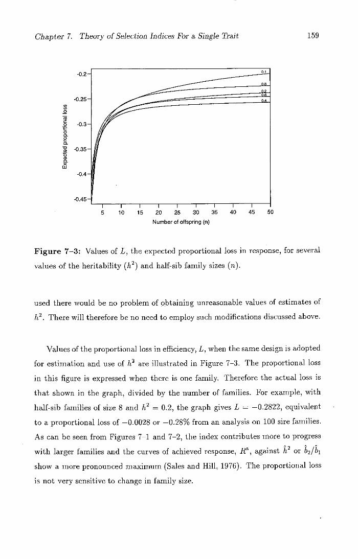
Chapter 7. Theory of Selection Indices For a Single Trait 159
(0 0 0
C 0 t 0 a 0
0.
•0 'I) 0 a) a 'C uJ
5 10 15 20 25 30 35 40 45 50
Number of offspring (n)
Figure 7-3: Values of L, the expected proportional loss in response, for several
values of the heritability (h 2 ) and half-sib family sizes (n).
used there would be no problem of obtaining unreasonable values of estimates of
h 2 . There will therefore be no need to employ such modifications discussed above.
Values of the proportional loss in efficiency, L, when the same design is adopted
for estimation and use of h 2 are illustrated in Figure 7-3. The proportional loss
in this figure is expressed when there is one family. Therefore the actual loss is
that shown in the graph, divided by the number of families. For example, with
half-sib families of size 8 and h 2 = 0.2, the graph gives L = — 0.2822, equivalent
to a proportional loss of —0.0028 or —0.28% from an analysis on 100 sire families.
As can be seen from Figures 7-1 and 7-2, the index contributes more to progress
with larger families and the curves of achieved response, W, against h 2 or
show a more pronounced maximum (Sales and Hill, 1976). The proportional loss
is not very sensitive to change in family size.
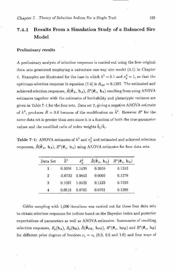
Chapter 7. Theory of Selection Indices For a Single Trait 160
7.4.1 Results From a Simulation Study of a Balanced. Sire
Model
Preliminary results
A preliminary analysis of selection responses is carried out using the four original
data sets generated employing a nnivariate one-way sire model (4.1) in Chapter
4. Examples are illustrated for the case in which h 2 = 0.1 and C2 = 1, so that the
optimum selection response in equation (7.4) is R.pt = 0.1292. The estimated and
achieved selection responses, R(OA, bA), W(0 0 , bA) resulting from using ANOVA
estimates together with the estimates of heritability and phenotypic variance are
given in Table 7-1 for the four sets. Data set 2, giving a negative ANOVA estimate
of h 2 , produces E = 0.0 because of the modification on A 2 . However R" for the
same data set is greater than zero since it is a function of both the true parameter
values and the modified ratio of index weights b2 /b1 .
Table 7-1: ANOVA estimates of It 2 and 0.2 and estimated and achieved selection
responses, R(OA, bA), R'(90, bA) using ANOVA estimates for four data sets.
Data Set j2 ar 2 E(AA, bA) f(0 0 , b)
1 0.3058 1.1439 0.3659 0.1243
2 -0.0732 0.9843 0.0000 0.1279
3 0.1097 1.0429 0.1433 0.1292
4 0.0518 0.9785 0.0701 0.1288
Gibbs sampling with 1,000 iterations was carried out for these four data sets
to obtain selection responses for indices based on the Bayesian index and posterior
expectations of parameters as well as ANOVA estimates. Summaries of resulting
selection responses, R(bA), R(b2), E(ÔPE, bpE), R"(6 0 , bJE) and R'(90, bB)
for different prior degrees of freedom v 5 = lie (0.0, 0.5 and 1.0) and four ways of

Chapter 7. Theory of Selection Indices For a Single Trait 161
implementing Gibbs sampling (see Section 4.7.1 for the implementation of Gibbs
sampling) are given in Table 7-2. As can be seen from this table the estimated and
posterior expected responses are very low when the prior degrees of freedom are
zero suggesting the Gibbs samples entered a black hole explained in Section 4.5.3.
Overall there does not seem to be any difference between the way in which the
Gibbs sampler is implemented. Hence the simplest, implementation 1, is chosen
for further analysis and making inferences about selection responses. Selection
progress, namely R(bA) is chosen for illustrative purposes. Marginal posterior
densities corresponding to this selection response for four data sets are shown in
Figure 7-4. As can be noted from Figure 7-4, marginal posterior densities look
almost like the densities of h 2 in Figure 4-8.
In Tables 7-1, and 7-2, selection responses shown with a hat, P, are obtained
from estimative procedures, either using ANOVA or Bayesian estimates. They
indicate how well an animal breeding practitioner thinks he will do. Therefore the
results from these responses overestimate the optimum selection response, 11opt•
On the other hand, selection responses denoted by H' are more realistic than
R since they give implication of how much one has achieved from the selection.
Consequently, the results of the achieved responses, H', are less than or close to
the optimum response. The responses with a subscript p, R, are more realistic
compared with the estimated responses, R. One can be expected to obtain the
most realistic selection response from using Bayesian point prediction procedure,
R"(9 0 , bpE). The responses obtained from estimates of the parameters such as
P(bA, bA) and E(b 2 , bpE) and also W(9 0 , bB) in Table 7-2 do not give
\realistic results and can therefore be excluded from any comparison. When
making comparisons between different alternatives of selection responses, it is
sensible to use the achieved responses from ANOVA estimates and Bayesian
point estimates when v3 = il, = 1, R(9 0 , bA) and H'(9 0 , bpE), respectively. It
can be clearly seen from Tables 7-1 and 7-2 that achieved responses from Bayesian
point estimates, H'(9 0 , bpE) give much superior results over the corresponding
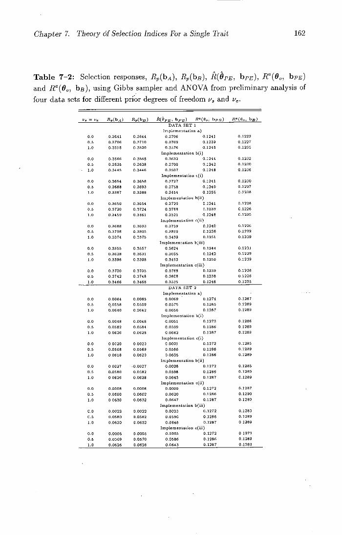
Chapter 7. Theory 61 Selection Indices For a Single Trait 162
Table 7-2: Selection responses, R2 (bA), R(bB), .ñ(ÔPE, bp-,), R 0 (00 , bpE)
and R0 (0 0 , b2), using Gibbs sampler and ANOVA from preliminary analysis of
four data sets for different prior degrees of freedom v 3 and V 6 .
= y e R,(b) Rp(bB) A(9p 5 , bp5) R(O 0 , bpp) Ra(8, b5)
DATA SET 1
Implementation a)
010 0.3641 0.3644 0.3706 0.1243 0.1229
0.1 0.3706 0.3710 0.3769 0.1239 0.1227
1,0 0.3518 0.3520 0.3576 0,1246 0.1235
Implementation b(i)
0.0 0.3566 0.3568 0.3632 0.1244 0.1232
0.5 0.3635 0.3638 0.3700 0,2242 0.1230
1,0 0.3445 0.3446 0.3507 0,1248 0.1236
Implementation c(i)
0.0 0.3654 0,3658 0.3727 0,1241 0.1230
0,5 0.3688 0.3693 0,3758 0,1240 0.1227
1,0 0,3387 0,3388 0,3454 0.1250 0,1238
Implementation b(ii)
0,0 0,3650 0,3654 0,3720 0.1241 0,1228
0.5 0,3720 0,3724 0,3788 0,1239 0.1226
1,0 0.3459 0,3461 0.3521 0,1248 0,1235
Implementation c(ii)
0,0 0,3688 0,3693 0,3759 0,1240 0,1226
0.5 0,3798 0.3805 0,3869 0.1236 0.1222
1,0 0,3374 0.3375 0,3439 0,1251 0,1239
Implementation b(iii)
0,0 0,3555 0,3557 0,3624 0,1244 0,1231
0.5 0,3628 0,3631 0.3695 0,1242 0,1229
1,0 0,3398 0,3398 0,3459 0,1250 0,1239
Implementation c(iii)
0,0 0,3700 0.3705 0,3768 0,1239 0,1226
0.5 0.3742 0,3748 0,3808 0.1238 0,1226
110 0.3466 0,3468 0,3535 0.1248 0.1235
DATA SET 2
Implementation a)
0.0 0,0064 0.0065 0,0069 0,1274 0,1287
0.5 0.0558 0,0559 0.0575 0,1285 0.1289
1,0 0,0640 0.0642 0,0656 0,1287 0,1289
Implementation b(i)
0,0 0,0048 0,0048 0,0051 0,1273 0,1286
0.5 0,0582 0,0584 0,0599 0,1286 0.1289
1,0 0.0626 0,0628 0.0642 0,1287 0,1289
Implementation c(t)
010 0.0020 0.0020 0.0021 0,1272 0,1285
015 0,0568 0,0569 0.0586 0,1286 0,1289
1.0 0,0618 0,0620 0.0635 0.1286 0,1289
Implementation b(ii)
0.0 0.0027 .0.0027 0.0028 0,1272 0,1285
0.5 0,0580 0,0582 0,0598 0,1286 0,1289
1.0 0.0626 0,0628 0,0643 0,1287 0,1289
Implementation c(ii)
0,0 0,0008 0,0008 0,0009 0,1272 0,1287
0,5 0,0600 0,0602 0,0620 0,1286 0.1290
1,0 0,0630 0.0632 0,0647 0.1287 01289
Implementation b(iii)
0,0 0,0022 0,0022 0,0023 0,1272 0,1283
0,5 0,0580 0,0582 0,0596 0.1286 0,1289
1.0 0,0630 0,0632 0,0648 0.1287 0.1289
Implementation c(iii)
0.0 0,0005 0.0005 0,0005 0,1272 01279
0.5 0,0569 0.0570 0,0586 0,1286 0,1289
2.0 0,0626 0,0628 0,0643 0,1287 0,1289

Chapter 7. Theory of Selection Indices For a Single Trait 163
Selection responses, R(bA), R(b), E(PE, bpE), (8 0 , bps) and R'°(6 0 , bB),
using Gibbs sampler and ANOVA from preliminary analysis of four data sets for
different prior degrees of freedom v 3 and v6 .
continued from Table 7-2....
U, = v, R,(b) R,(bB) i1<PE, bpE) R'(O, bps) fla(90, b0)
DATA SET 3
Implementation a)
0.0 0.0623 0.0624 0.0691 0.3287 0.1290
0.5 0.1562 0.1567 0.1623 012291 0.1286
1.0 0.1387 0.1388 0.1433 012292 0.1289
Implementation b(i)
0,0 0,0441 0,0441 0.0500 0.1284 0,1289
0,5 0,1528 0,1532 0.1590 0,1291 0,1287
1.0 0,1412 0.2434 0.1466 0.1292 0.1289
Implementation c(i)
0.0 0,0478 0.0479 0.0535 0,1284 0.1210
0.5 0.1625 0.1632 0.1693 0,1290 0.1285
1,0 0.1440 0,1442 0,1497 - 0,1292 0.1288
Implementation b(ii)
0,0 0,0342 0.0342 0,0389 0,1281 0,1290
0.5 0,1534 0,3538 0,1601 0.1291 0,1286
1,0 0,1407 0,3409 0.1458 0.1292 0,1289
Implementation c(ii)
0.0 0.0190 0,0190 0.0221 0.1278 0.1290
0.5 0,1563 0,1569 0.1635 0.1291 0.12
1.0 0.1353 0.1354 0.1401 01292 0.1290
Implementation b(iii)
0,0 0.0327 0.0327 0.0373 0,1281 0.1290
015 0.1536 0.1540 0.1599 0,1291 0.1286
1,0 0,1416 0.1418 0.1469 0,1292 0.1289
Implementation c(iii)
010 0,0231 0.0231 0.0270 0,1279 0.1288
0,5 0.1497 0.1500 0,1559 0.1291 0.1287
1,0 0.1386 0.1388 0.1438 0,1292 0,1289
DATA SET 4
Implementation a)
0,0 0,0269 0,0269 0,0293 0.1280 0,1291
0,5 0,0993 0.0998 0,1037 0,1211 0,1292
1,0 0,0942 0,0144 0.0973 0,1211 0.1292
Implementation b(i)
0,0 0,0173 0.0173 0,0195 0,1277 0.1292
0.5 0,1043 0.1049 0,1091 0,1291 0.1291
1,0 - 0,1007 0.1012 0,1048 0,1291 0,1292
Implementation 0(i)
0,0 0.0112 0.0112 0,0127 0,1275 0,1292
0.5 0,1079 0.1085 0,1127 0,1292 0.1291
1,0 0,1054 0.1059 0,1095 011291 0.1292
Implementation b(ii)
0.0 0.0098 0.0099 0.0111 0.1275 0.1292
0,5 0,1061 0.1067 0.1110 0.1291 0.1291
1.0 011021 0.1025 0,1061 0.1291 0,1292
Implementation c(ii)
0,0 0.0150 0.0150 010171 0,1276 0,1292
0.5 0,1032 0,1038 0.1084 0,1291 0,1291
1,0 0,1028 0,1032 0.1068 0,1291 0,1292
Implementation b(iii)
0,0 0,0109 0,0110 0,0124 0,1275 0.1292
0.5 0.1067 0,1073 0,1114 0,1292 0,1291
1,0 0.1030 0,1035 0,1072 0.1291 0.1292
Implementation c(iii)
0,0 0,0064 0,0064 0,0073 0,1274 0.1292
0.5 0,1053 0.1059 0,1104 0,1291 0,1291
1,0 0,1043 0.1048 0,1085 0.1291 0,1292

Chapter 7. Theory of Selection Indices For a Single Trait 164
0 C 0 C
3
0.0 0.1 0.2 0.3 0.4 0.5 0.6 0.7
Selection response
Figure 7-4: Posterior density of selection response, R(bA), from Gibbs sampling
based on 1,000 iterations, and the estimates of index weights from ANOVA for
data sets 1, 2, 3 and 4.
achieved responses from ANOVA estimates, Ra(00, bA) for all four data sets when
=V, = 1.
Results with 500 replicate samples
In the main part of the analysis, 500 data sets were generated using different
numbers and sizes of families (s = 10, 25, 80, n = 8, 16, 20) and heritabilities
(h 2 = 0.1, 0.3, 0.6) (see Section 4.7.2 for detailed information on data sets and
designs). For each set, ANOVA results were obtained and Gibbs sampling cycles
were carried out with 1,000 iterations. Table 7-3 gives the optimum selection
responses, R opt , for these family sizes and heritabilities. As both h2 and n increase
the optimum response also increases.
2
4

Chapter 7. Theory of Selection Indices For a Single Trait 165
Table 7-3: Optimum selection responses, for ii = 8, 16, 20 and h 2 = 0.1,
0.3, 0.6.
It 2 n=8 n=16 n=20
0.1 0.1144 0.1252 0.1292
0.3 0.3219 0.3332 0.3367
0.6 0.6119 0.6161 0.6172
Means and standard deviations of the estimated and achieved responses,
bA) and w(0 0 , hA), using ANOVA estimates over 500 replicates for different
heritabilities and family sizes are shown in Table 7-4. Comparison with Table
7-3 indicates that there is a tendency to overestimate the optimum progress,
R02 , by using the estimated response obtained from using ANOVA estimates,
R(OA, bA). This bias is considerable when there are few families but becomes
fairly small with amounts of data sufficient to give reasonably good calculated
indexes. R is very sensitive to the value of h 2 since E is roughly proportional
to h 2 and also the estimate, â,, of the phenotypic standard deviation. As h
and n increase it seems that the discrepancy between R and R,pt gets smaller
and for larger families there seem to be some underestimates. Conversely, the
achieved response R"(0 0 , hA) using ANOVA estimates appears to underestimate
the optimum progress indicating a downward bias. This response converges to the
optimum response R.pt as the family size increases. Also the difference between
11 and R gets smaller.
Mean selection responses for RP(bA), R(bB), h(è 2 , bpE), R"(9 0 , bp—P) and
W(9 0 , b2) over 1,000 iterations of 500 replications for different values of her-
itability and family sizes are shown in Table 7_5 The same conclusion made
for R(OA, hA) and W(9 0 , b 4 ) obtained using only ANOVA estimates can also
be drawn here. The results of these tables indicate that R(bA), R(bB) and

Chapter 7. Theory of Selection Indices For a Single Trait
166
Table 7-4: Means and standard deviations (SD) of predicted and achieved selec-
tion responses, R(OA, IDA), R'(00, bA) using ANOVA estimates over 500 replicates
for different heritabilities and family sizes.
E(è4 , bA) R"(80 , bA) h 2 Mean SD Mean SD
S=10 n=8 0.1 0.1704 0.2276 0.1133 0.0025 0.3 0.3237 0.3061 0.3176 0.0058 0.6 0.6165 0.4546 0.5975 0.0146
s=10 n=16 0.1 0.1350 0.1443 0.1236 0.0022
0.3 0.3135 0.2273 0.3260 0.0074 0.6 0.5772 0.3453 0.5966 0.0248
s=10 11=20 0.1 0.1476 0.1449 0.1273 0.0028 0.3 0.3212 0.2117 0.3295 0.0082 0.6 0.6230 0.3355 0.5997 0.0232
s=25 n=8 0.1 0.1302 0.1461 0.1139 0.0011 0.3 0.3202 0.2049 0.3193 0.0028
0.6 0.6145 0.2808 0.6053 0.0087 s=25 n=16
0.1 0.1233 0.0957 0.1244 0.0009 0.3 0.3197 0.1445 0.3299 0.0040 0.6 0.6243 0.2098 0.6097 0.0088
s=25 n=20 0.1 0.1233 0.0933 0.1283 0.0012 0.3 0.3380 0.1360 0.3332 0.0045
0.6 0.6108 0.1889 0.6110 0.0092 s=80 n=8
0.1 0.1211 0.0952 0.1142 0.0004 0.3 0.3205 0.1216 0.3209 0.0015 0.6 0.6002 0.1547 0.6096 0.0033
s=80 n=16 0.1 0.1205 0.0604 0.1248 0.0004
0.3 0.3291 0.0772 0.3322 0.0014 0.6 0.6199 0.1141 0.6141 0.0029
s=80 n=20 0.1 0.1257 0.0519 0.1289 0.0004
0.3 0.3343 0.0680 0.3357 0.0013 0.6 0.6174 0.1133 0.6150 0.0028

Chapter 7. Theory of Selection Indices For a Single Trait 167
Table 7-5: Summary of selection responses using Gibbs sampler and ANOVA
methods, R(bA), R 2 (bB), E(APE, bpE), W(6 0 , bp-r) and R"(0 0 , bB), with
k = 1,000 and rn = 500 for different heritabilities and family sizes.
Rp(bA) R(b5) E(bpE, bpE) R"(00 , bpE) R"(0 0 , b)
h2 Mean SD Mean SD Mean SD Mean SD Mean SD
slO n=8
0.1 0.1988 0.0865 0.1999 0.0868 0.2070 0.0884 0.1140 0.0009 0.1128 0.0014
0.3 0.3537 0.1145 0.3566 0.1148 0.3639 0.1147 0.3210 0.0016 0.3200 0.0023
0.6 0.5152 0.1306 0.5216 0.1338 0.5272 0.1329 0.6090 0.0033 0.6105 0.0017
s10 n=16
0.1 0.1750 0.0800 0.1766 0.0795 0.1849 0.0814 0.1243 0.0016 0.1231 0.0023
0.3 0.3512 0.1299 0.3545 0.1280 0.3624 0.1267 03310 0.0030 0.3304 0.0037
0.6 05350 0.1540 0.5400 0.1524 0.5446 0.1502 0.6105 0.0075 0.6124 0.0051
slO n=20
0.1 0.1822 0.0905 0.1837 0.0900 0.1926 0.0916 0.1280 0.0023 0.1268 0.0030
0.3 0.3584 0.1301 0.3613 0.1285 0.3696 0.1270 0.3340 0.0036 0.3336 0.0042
0.6 0.5614 0.1513 0.5659 0.1509 0.5699 0.1483 0.6117 0.0077 0.6133 0.0054
s=25 11=8
0.1 0.1605 0.0794 0.1608 0.0794 0.1648 0.0808 0.1141 0.0007 0.1137 0.0011
0.3 0.3366 0.1278 0.3374 0.1274 0.3420 0.1273 0.3208 0.0015 0.3204 0.0020
0.6 0.5601 0.1501 0.5616 0.1508 0.5643 0.1496 0.6093 0.0034 0.6101 0.0023
s25 n=16
0.1 0.1425 0.0608 0.1429 0.0607 0.1474 0.0621 0.1248 0.0008 0.1244 0.0011
0.3 0.3363 0.1206 0.3370 0.1203 0.3418 0.1197 0.3311 0.0025 0.3311 0.0028 -
0.6 0.5985 0.1433 0.5992 0.1435 0.6011 0.1419 0.6125 0.0054 0.6131 0.0043
s=25 n20
0.1 0.1419 0.0648 0.1422 0.0647 0.1466 0.0658 0.1287 0.0011 0.1284 0.0014
0.3 0.3516 0.1210 0.3521 0.1208 0.3568 0.1200 0.3341 0.0032 0.3341 0.0034
0.6 0.5985 0.1371 0.5992 0.1370 0.6010 0.1355 0.6135 0.0058 0.6140 0.0047
s=80 n=8
0.1 0.1305 0.0606 0.1306 0.0605 0.1324 0.0612 0.1143 0.0003 0.1142 0.0004
0.3 0.3190 0.1056 0.3191 0.1056 0.3214 0.1054 0.3212 0.0011 0.3212 0.0012
0.6 0.5915 0.1353 0.5916 0.1353 0.5925 0.1346 0.6100 0.0025 0.6103 0.0021
s=80 n=16
0.1 0.1225 0.0454 0.1226 0.0454 0.1244 0.0458 0.1250 0.0003 0.1249 0.0004
0.3 0.3296 0.0752 0.3296 0.0752 0.3315 0.0750 0.3323 0.0012 0.3323 0.0012
0.6 0.6235 0.1066 0.6236 0.1066 0.6241 0.1061 0.6144 0.0024 0.6144 0.0023
srz8O n20
0.1 0.1252 0.0428 0.1253 0.0428 0.1271 0.0431 0.1290 0.0003 0.1289 0.0004
0.3 0.3362 0.0674 0.3362 0.0674 0.3380 0.0672 0.3358 0.0013 0.3358 0.0012
0.6 0.6226 0.1069 0.6227 0.1068 0.6232 0.1063 0.6152 0.0024 0.6153 0.0023
Chapter 7. Theory of Selection Indices For a Single Trait 168
P(ÔPE, bpE) are inseparable giving similar results. The index based on the pos-
terior expectation of h2 , R"(6 0 , bpE), gives higher achieved responses than that
based on the ANOVA estimates for all designs. The Bayesian index W(0 0 , bn)
appears superior to the AN OVA index except for the cases with small family sizes
and h2 = 0.1, and superior to that based on the posterior expectation of h 2 when
It 2 is 0.6. This can be shown more clearly by constructing a table of proportional
loss in efficiency.
The values of expected (i.e. mean) losses in response achieved using estimates
of parameter values relative to that from the optimum index are given for responses
W(0 0 , bA), R"(6 0 , bpE) and R (6, bB) in Table 7-6. In this table smaller values
of [E(W)—R0]/R0% indicate less efficient situations for index construction. The
trends associated with increases in .s and n indicate that, with more data, more
reliable selection indexes may be constructed. For the parameter set chosen the
loss in efficiency is rather small: a 0.1 - 3 % reduction in genetic gain for a range
of heritabilities.
Comparisons may be made in Table 7-6 between the various combinations of
family number and size involving the same total number of observations. For ex-
ample, the two combinations, 10 sires with 20 offspring and 25 sires with 8 offspring
involve a total of 200 offspring. These results indicate that, for the combination
of parameters considered here and for a fixed total number of observations, 8 off-
spring per sire group leads to more efficient selection. It is possible to see this
more clearly for fixed heritability and number of families, s, with varying number
of offspring per sire (Ii = 8, 16 20). The trends associated with this situation
suggest that the most effective selection can be obtained using 8 offspring per sire
group. For a fixed number of offspring (ii) and of heritability, the proportional
loss in efficiency tends to increase swiftly with an increase in the mberfmily /
(s).
As can be seen from Table 7-6, the achieved response using ANOVA esti-
Chapter 7. Theory of Selection Indices For a Single Trait 169
mates R'(90, bA) gives the highest expected loss. The lowest proportional loss in
efficiency is observed in W(9 0 , byE). For designs with small family size, the dis-
crepancy between the values of proportional losses obtained from using ANOVA
estimates and posterior expectations in Table 7-6 appears to be rather large. How-
ever, with an increase in the family size these values for responses R'(60, IDA) and
W(0 0 , bB) give similar results.
The estimate of progress, I?, depends critically on what value of the estimate h 2
of heritability is used and Sales and Hill (1976) showed that the standard error of I?
is similar in magnitude to the standard error of h 2 . This can be easily seen when
compared the standard deviation of ANOVA estimates of h 2 in Table 4-7 with
that of E(OA, bA) in Table 7-4 and the standard deviation of marginal posterior
expectations for h 2 in Table 4-8 with those of R(bA), R(bB), 9 PE, byE) and
R(OpE, bE) in Table 7-5. For example, with 20 half-sib families of size 16 and
the true heritability 0.3 the standard deviation of E obtained from simulation and
Gibbs sampling was found to be between 0.12 and 0.14 in Tables 7-4, 7-5; the
optimum response for this particular experiment is 0.3332 (see Table 7-3). For
the same experiment the standard deviation of estimates of h 2 was shown to be
exactly the same as that of E (see Tables 4-7 and 4-8).
7.5 Discussion
Two major points are illustrated in this chapter. Firstly, it is possible to use a
decision theory approach to obtain an assessment of the genetic merit of half-
sib families for a single trait. Secondly, the assessment from this approach is
contrasted with conventional procedures.
It has been assumed that prior information is available on the population
from which the candidates are drawn and such information is incorporated in the
analysis using Bayesian decision procedures. The method of estimation based

Chapter 7. Theory of Selection Indices For a Single Trait 1 170
Table 7-6: Proportional loss in efficiency, L = [E(W) - R0]/R0%, in an index
of individual and family mean performance when the heritability ( h 2 ) is estimated
from s families of the same size it. Values were computed for three different
achieved responses, L'(90, bA), L"(9 0 , bpE) and L"(9 0 , bB).
Proportional Loss (7o) h2 L°(9 0 , bA) I/'(O, bpE) L"(0 0 , bB)
s=10 n=8 0.1 -1.0312 -0.3758 -1.4245 0.3 -1.3540 -0.3075 -0.6180 0.6 -2.3580 -0.4788 -0.2337
s=10 n=16 0.1 -1.2460 -0.6871 -1.6459 0.3 -2.1667 -0.6662 -0.8463 0.6 -3.1600 -0.9041 -0.5957
s=10 n=20 0.1 -1.4550 -0.9135 -1.8424 0.3 -1.2297 -0.7931 -0.9119 0.6 - -2.8307 -0.8863 -0.6271
s=25 n=8 0.1 -0.4632 -0.2884 -0.6379 0.3 -0.8354 -0.3696 -0.4938 0.6 -1.0830 -0.4298 -0.2991
s=25 n=16 0.1 -0.6310 -0.2876 -0.6070 0.3 -0.9963 -0.6303 -0.6273 0.6 -1.0340 -0.5795 -0.4821
s=25 n=20 0.1 -0.6812 -0.3716 -0.6038 0.3 -1.0310 -0.7692 -0.7900 0.6 -0.9997 -0.5946 -0.5136
s=80 n=8 0.1 -0.1836 -0.1136 -0.1836 0.3 -0.3385 -0.2330 -0.2299 0.6 -0.3808 -0.3154 -0.2664
s=80 n=16 0.1 -0.2876 -0.1278 -0.2077 0.3 -0.3061 -0.2731 -0.2611
0.6 -0.3198 -0.2711 -0.2711 s=80 n=20
0.1 -0.2709 -0.1393 -0.2012
0.3 -0.2881 -0.2792 -0.2703 0.6 -0.3516 -0.3192 -0.3030
Chapter 7. Theory of Selection Indices For a Single Trait 171
on ANOVA do not lead to a selection procedure which is in any sense the best.
Therefore estimative methods can differ substantially from those based on prior
distributions and the former can be seriously misleading for designs with small
family size.
However, with an increase in the family size, both conventional and Bayesian
methods give similar results of selection responses. This similarity of the assess-
ment of the genetic merits by the conventional method and by the decision theory
method is not unexpected for the large sample sizes. When a single trait is being
selected for, there is little scope for genetic improvement over individual selection
by using selection index. As a result, we would not expect to find a great deal
of difference in the group of animals selected using different methods or individ-
ual performances of the animals. Further, for designs with large sample size, the
asymptotic equivalence of the Bayes solution and the decision which maximizes
the expected posterior utility at the value of maximum likelihood estimate of 9
becomes evident. Hence, the conventional method and the decision theory would
give very similar results. When the selection is for more than one trait, the de-
cision theory method is expected to give results which differ from the selection
using a conventional multi trait index. This case is considered in Chapter 9.
Chapter 8
Multiple-Trait Analysis in Animal
Breeding
8.1 Introduction
Multivariate analysis is the branch of statistics dealing with the summarization,
representation, and interpretation of data sampled from populations in which
each experimental unit is. measured for more than one characteristic. The ex-
perimenter's justification for measuring several responses on each unit is that no
single response adequately characterizes the individual, or discriminates among
individuals, with respect to whatever criterion is employed. The engineer may
measure weight, length, tensile strength, and hardness on each of several items
manufactured by a given process. The agronomist might be concerned with yield,
stand, strength, and disease resistance when testing new plant varieties. The
dairy scientist may measure milk yield, fat percentage, feed intake, and weight
change on each cow in evaluating a feeding program. In short, most processes
of experimentation are multivariate. Further, since the several measurements on
each experimental unit are often correlated, it is inappropriate to apply univariate
analysis separately to each of the response variables. Univariate analysis is rather
a simplification open to the experimenter who happens to be measuring only one
characteristic as his experimental material.
In general, the practical objective of animal breeding is to achieve genetic
improvement of livestock by selection of breeding animals. The selection is almost
172

Chapter 8. Multiple-Trait Analysis in Animal Breeding 173
invariably based on more than one economically important trait measured on each
individual. For example, selection for milk production traits is usually on some
combination of breeding values for milk, fat and protein. Therefore multiple trait
model is a natural choice for analysis of those observations.
In the statistical analyses of animal breeding data, traits on the same individu-
als are often considered one at a time. Milk production traits, which are known to
be strongly correlated, are evaluated separately in most countries for the sire eval-
uation. Usually we are interested, however, not only in the mode of inheritance
of a particular trait but also in its relationships with other traits and correlated
responses when selecting on the trait analysed. Multivariate analyses are required
to obtain estimates of genetic and phenotypic correlations between traits. More-
over, while univariate analyses ignore correlations between traits, joint analyses of
correlated traits utilize information from all traits to obtain estimates for a spe-
cific trait and should therefore yield more accurate results. This is of particular
relevance when data are not a random sample, i.e., if records for some traits are
missing as a result of selection. For animal breeding data, this is often the case
since, typically, data originate from selection experiments or are field records from
livestock improvement schemes which select animals on the basis of performance.
In that situation, univariate analyses are expected to be biased while multivariate
analyses may account for selection (Meyer, 1991). The obvious disadvantage of
multiple-trait analyses is generally the additional computational requirements due
to the increased number of equations to be solved. To reduce computational and
storage requirements canonical transformations can be employed. The less obvious
disadvantage (for the conventional theory) is that the more traits are analysed the
greater the probability of estimates outside (or on the boundary of) the parameter
space.
Benefit from multiple-trait analysis Advantages in the joint consideration of
several traits in genetic evaluations essentially come from the following points.

Chapter 8. Multiple-Trait Analysis in Animal Breeding 174
Multiple-trait procedures use more information to evaluate individuals com-
pared with univariate methods. The absolute values of genetic and envi-
ronmental correlations may be high. Therefore by considering all traits
simultaneously the accuracy of estimation and prediction, and consequently
response to selection are increased. The gain in accuracy of selection due
to multiple-trait evaluations depends on the absolute values of genetic and
residual correlations, on the difference between genetic and residual correla-
tions and on progeny group size.
Some traits are measured on a limited number of individuals, and estimation
accuracy may be gained by analysing these traits jointly with other traits
which are measured on more individuals in the population. Some individuals
may lack records on some traits as a result of selection on one or more
other traits. For example, in beef cattle, calves are selected at weaning for
their weaning weights prior to further testing, and at yearling age they are
measured for yearling weights and/or gains on test. Suggestions have been
made that the use of multiple trait analysis for a simultaneous analysis of
selected and unselected data would reduce the selection bias due to selection
on a correlated trait.
Variance and covariance components are used by quantitative geneticists as
measures of genetic and environmental relationships between two or more charac-
ters. Estimation of the components is also required to formulate animal breeding
schemes. In the corresponding univariate case, variance components are estimated
by equating various sums of squares to their expectation. Obviously this process is
extended to the multivariate case to estimate covariance components by equating
the sums of cross-products to their expectations. Methods of estimation based
on differences between mean squares or between matrices of mean squares and
products can lead to unreasonable estimates, such as estimated genetic variance
matrices which are not positive definite (Hill and Thompson, 1978). Some ad hoc

Chapter 8. Multiple-Trait Analysis in Animal Breeding 175
modification is needed to such estimates before they can be used to construct a
selection procedure. A method termed bending was described and evaluated in
animal breeding situations by Hayes and Hill (1981). Details of their approach
will be given later in this chapter.
Analysis of variance (ANOVA) type methods have been widely used to estimate
genetic and phenotypic parameters and to formulate animal breeding schemes.
ANOVA methods require records for all traits for all individuals. If animals with
missing records are omitted from the analysis, then part of the information avail-
able is ignored. More importantly, if lack of records is the outcome of selection
based on some criterion correlated with traits under analysis, estimates are likely
to be biased by selection. In contrast, procedures based on maximum likelihood
(ML) utilize all records available and, under certain conditions, account for selec-
tion. Even if these conditions are only partially fulfilled, ML estimates are often
considerably less biased by selection than their ANOVA counterparts (Meyer and
Thompson, 1984).
A modified ML procedure, so-called restricted (or residual) maximum likeli-
hood (REML) was described for a univariate analysis by Patterson and Thompson
(1971). It accounts for the loss in degrees of freedom due to fixed effects in the
model of analysis, and has become the preferred method of analysis for animal
breeding data, not least for its property of reducing selection bias. Thompson
(1973) extended this procedure to the case of multivariate two-way classification
with treatments as fixed effects and blocks as random effects where the design
and block structure were the same for all variates. His multiple-trait 'REML es-
timator requires all traits to be measured on all animals. A multivariate REML
algorithm suggested by Meyer (1985) describes a procedure for a mixed two-way
classification with the same design matrix for all traits, using a transformation of
the variates to a canonical scale. Meyer (1991) then describes the extension of
univariate REML estimates of variance and covariance components to multivari-
ate analyses, allowing for missing records. These multivariate REML algorithms,

Chapter 8. Multiple-Trait Analysis in Animal Breeding 176
however, in general require the direct inverse of a matrix of size equal to the total
number of levels of random effects multiplied by the number of traits considered
simultaneously (Meyer, 1991). This represents not only a substantial computa-
tional requirement but imposes several limitations on the model and dimension of
analysis. Also practical applications are feasible only if a special data structure
can be exploited. Even then the analysis is usually limited by the size of the matrix
to be inverted, which is proportional to the number of traits (Meyer, 1985).
So far, we have demonstrated that the Gibbs sampling procedure can be used
successfully to carry out Bayesian analysis of all parameters in a balanced univari-
ate one-way sire model assuming a half-sib family structure in several chapters.
A multivariate empirical Bayes approach for I polygenic binary traits is consid-
ered assuming improper priors for fixed and random parameters by Foulley et al.
(1987) (see Table 3-1). They considered a situation where the values of the dis-
persion parameters are not known and are replaced by point estimates obtained
from their marginal posterior distribution. However, many of the traits in animal
breeding applications present continuous distribution of phenotypes and multi-
variate analyses of such traits have not been carried out within the framework
of Bayesian procedures. The objective of this chapter is to extend the general
principle of the Bayesian scheme for a univariate one-way classification in Chap-
ter 4 to a balanced multiple-trait one-way sire model assuming a half-sib family
structure. Unlike Foulley et al. (1987), informative priors are used for random
parameters to make Bayesian marginal inferences about variance components and
functions of them. The results of Gibbs sampling are compared with estimates of
the parameters obtained from the analysis of variance method with and without
modification using the bending technique of Hayes and Hill (1981).

Chapter 8. Multiple-Trait Analysis in Animal Breeding 177
8.2 Variance Components Estimation in a Bal-anced Multivariate One-way Classification
In a one-way multivariate analysis of variance with random sire effects, the between-
groups (between-sires) variance-component matrix is estimated from the difference
between the between-groups and within-groups mean square and product matri-
ces. This variance matrix is used to estimate heritabilities, genetic variances,
covariances and correlations and in the construction of selection indices.
8.2.1 The model and assumptions
Consider a balanced one-way classification with .s half-sib groups of equal size
n, and t traits recorded on each individual. Observations are here assumed to
be multivariate normally distributed with the between- and within-group effects
independent of each other. Let y ij denote the vector of values of the t traits
observed on the jth animal in the ith sire group (i = 1,.. . , 8; j = 1,.. . ,ri). Then
the multivariate linear random effects model can be given by
y ij i=l .... ,s; j=1,...,n. (8.1)
where p is a t-vector of expectations, Si is a t-vector of sire effects and e ij is
a vector of t departures (residual error terms) representing the variation within
half-sib families.
The vectors of random sire effects, s, and residuals e ii are assumed to be
independently and normally distributed. The s i are taken to be N(O, E 3 ) and
the.e ij to be N(O, with E e positive definite. The vectors Yij are thus jointly
multivariate normal with expectation vector p and second moments given by
Var(y) = = E. + E,
Cov(yjj, = = (i 54 a'),

Chapter 8. Multiple-Trait Analysis in Animal Breeding 178
Cov(y, y'') = 0 (i $
where E represents the phenotypic variance matrix and E 9 the genetic variance
matrix.
With these assumptions the following balanced one-way multivariate anal-
ysis of variance table with paternal half-sib groups with Var(y) = E and
Cov(y1 , y') = E9 can then be obtained
Source d.f. SSP MSP E(MSP)
Between-sires s - 1 Sb Mb - 1 E + 4 nE9 EP 4 9 = Ee + nE3
Within-sires .s(n - 1) S M — — 1 E E 9 - E
Here SSP denotes the sums of squares and products and MSP the mean squares
and products. Sb and S. represent the matrices of sums of squares and products
between and within groups and are given by the following formulae
Sb =
and
Sw
= E - - 1=1 j=1
where yi. is the mean vector for group i, and y.. is the overall mean vector.
Mb = Sb/(s - 1) and M = S/{s(ri - l)} are the matrices of mean squares
and products between and within groups corresponding to 5b and S,. The ma-
trices of sums of squares and products, 5b and S, are independent with central
Wishart distributions given respectively by
W[(s - 1), F m ]
and
r- Wj [s(n - 1), Eel

Chapter 8. Multiple-Trait Analysis in Animal Breeding 179
where r = E + nE 5 . Hence one can write the densities of Sb and S i,, as
(
1-2 1
f(Sb) H F s—i) exp tr (S br l )] ,
and
f(s) H e pIs(1) exp 1-2
tr (SE; 1 )] .
8.2.2 Estimated variance components and some restric-tions
From one-way multivariate analysis of variance, the estimated phenotypic, genetic,
sire and residual covariance matrices are respectively
= [Mb + (n - 1)M]/n, (8.2)
Eg = 4(Mb - M)/n, (8.3)
= (Mb - M)/n, (8.4)
and
= M. (8.5)
The multiple-trait half-sib sire model in (8.1) imposes some restrictions on
the variance matrices E 5 and E. In animal breeding applications, any linear
combination of traits c'y, say, has heritability 4c' 5 c/c'(J 5 + E)c, which is the
proportion of the variance observed in the parents that is transmittable to the
offspring. The constraint that heritability is no more than 1 for all such combi-
nations implies that E - 3E 5 is non-negative definite. A method of estimation
which ignores this restriction may lead to ridiculous estimates of heritability for
some traits or linear combinations of them.

Chapter 8. Multiple-Trait Analysis in Animal Breeding 180
8.2.3 Bending Theory
Hayes and Hill (1981) introduced a method, termed bending, to modify the esti-
mates of genetic and phenotypic variance matrices in animal breeding situations.
The method consists of adjusting the characteristic roots or eigenvalues of M'Mb
towards their mean. The bending of the estimates of genetic and phenotypic vari-
ance matrices shows some obvious analogies with the technique of ridge regression
suggested by Hoerl and Kennard (1970). The ridge regression estimation proce-
dure of Hoerl and Kennard (1970) used in multiple regression analysis is based on
adding a small quantity to each diagonal element of X'X to improve the estimates
of regression coefficients, where X is the design matrix. Campbell (1980) has also
suggested shrinkage of estimates in discriminant and canonical variate analysis
to improve markedly stability of the resulting coefficients (especially in canonical
variate analysis) when the between-groups sum of squares for a particular prin-
cipal component defined by the within-groups covariance or correlation matrix is
small and the corresponding eigenvalue is also small. Bending can be seen as an
example of a regularization method. Regularization reduces the variance associ-
ated with the sample-based estimate at the expense of potentially increased bias
(Friedman, 1989). In all of these cases the attempt is made to increase the relia-
bility of sample estimates through some suitable adjustment accepting the loss of
unbiasedness thereby caused.
Some modification of parameter estimates has always been practiced, at least
in Monte Carlo simulation studies, when it was obvious that the .estimates were
outside possible limits of the true values. Three examples are: negative estimates
of additive genetic variance, estimates of the additive genetic variance which are
greater than the estimates of phenotypic variance (heritability estimates greater
than one), and estimates of additive genetic correlations which are greater than
one in absolute magnitude. In such cases, it has been the usual practice to set the
estimates to the corresponding bound (Harris, 1964; Sales and Hill, 1976, 1977).
Chapter 8. Multiple-Trait Analysis in Animal Breeding 181
However it is definitely not proposed that this is the optimum modification pro-
cedure. For two or more variates, if the estimated between-group variance matrix
has positive diagonal elements, a matrix with one or more negative characteristic
roots implies ordinary or partial between-group, or genetic, correlations outside
the range -1 to +1 (Hill and Thompson, 1978). Although ordinary correlations
outside this range are displayed by a correlation matrix, impossible partial cor-
relations are more easily missed and procedures for putting several estimates to
their bounds simultaneously are less obvious and not necessarily satisfactory.
The approach of Hayes and Hill (1981) for modifying the parameter estimates
for several traits is based on the phenomenon that the roots of the between-group
MSP matrix Mb relative to the within-group MSP matrix M are biased away
from their expectations (Hill and Thompson, 1978) and is given as follows.
The roots, vk, of the the determinantal equation I Mb - VJCMW I= 0 or, equiv-
alently I M 1 M - vkI 1= 0 (Anderson, 1984) can be modified using the bending
approach. If it is assumed that there are many more degrees of freedom within
groups than between groups, the mean of the roots, of M 1 Mb is biased com-
pared with its expectation. In particular, the larger roots are biased upwards, the
smaller roots downwards, and pairs of equal roots with the same expectation are
spread excessively about their mean. This suggests that the roots of M 1 Mb from
the balanced one-way multivariate analysis of variance might usefully be regressed
towards their mean without altering the corresponding eigenvectors or the average
root (Hayes and Hill, 1981). The between-sire MSP matrix, M&, estimated with
relatively few degrees of freedom, is bent towards the within-sire mean product
matrix to obtain the modified between-group MSP matrix, M:
M = (1 - w)M,, + wUM, (8.6)
is an arbitrarily chosen bending factor in the range [0, 1] and ü denotes the mean
of the roots of M'Mb, with vk defined as above. M'M has characteristic roots
(1 - w)vk + WV.

Chapter 8. Multiple-Trait Analysis in Animal Breeding 182
The estimate of the residual variance matrix, t, is unchanged and the sire
variance matrix is modified as follows
= (M - M)/n.
The modified estimates of the phenotypic, genetic and variance matrices, E and
are obtained by replacing Mb in E and EL, with M&* to give
= {M+(n-1)M)}/n
= {(l—w)M5+(n-- 1+w)M}/n
tg = 4(M - M)/n
= 4{(1 - w)M 5 —(1— wU)M}/n.
E and E are non-negative definite only if (1 - w)vk + wD - 1 is >_ 0, i.e. only
if w > (1 - - 1)14. When w = 0, the t, and are the usual estimates;
when w = 1,
Mb =
= 4(t) - 1)M/n,
tP = (ü + Ti - l)M/n,
E. and E,, are proportional, i.e. E;E = ci, with c = 4(13 - 1)/(13 + ii - 1), and
M 1 M = 13(MM) = til.

Chapter 8. Multiple-Trait Analysis in Animal Breeding 183
8.3 Canonical transformations
The idea of linear transformation of correlated traits such that they become uncor-
related is not at all new. This idea is used in principal component and canonical
correlation analyses. A number of authors have considered the use of a canonical
transformation of the data to estimate variance components by REML for mul-
tivariate linear models with one random factor and equal design matrices for all
traits. This transformation was first suggested for animal breeding applications by
Thompson (1976, cited by Jansen and Mao, 1988). Hayes and Hill (1980) showed
how a canonical transformation of phenotypic and genetic variance matrices could
be useful for locating sampling properties of selection indices.
Now consider a transformation of the genetic and phenotypic variance matrices,
E9 and E,,, respectively. Since YL is a symmetric non-negative definite matrix
and EP is a symmetric positive definite matrix of the same order. By standard
multivariate theory (Anderson, 1984), there exists a nonsingular matrix E which
satisfies
= AandSE2E =1
where A denotes diag(Ak) (Ic = 1,... ,t). The roots ... > A, of the determi-
nantal equation
I - 1= 0
(or, equivalently, the characteristics roots of E 1 E) are all non-negative. Hayes
and Hill (1980) give a rationalisation and a numerical example for such a trans-
formation. Some general library program packages, e.g. Fortran NAG library,
provide routines for obtaining matrix S and Ak'5 by solving the determinental
equation.
For the multiple-trait sire model used in this study, records are assumed to
be available on all traits for the random effects. The canonical transformation

Chapter 8. Multiple-Trait Analysis in Animal Breeding 184
can then be applied to yield - -i a set of uncorrelated t new traits some-
times called canonical variables. The new phenotypic variables are uncorrelated
and each has unit variance. The new genotypic variables are also uncorrelated
and have variances, Ak. Because the phenotypic variances are all unity, the corre-
sponding heritabilities (called canonical heritabilities) are also equal to Ak. Hence
a multivariate analysis can be carried out as a series of t corresponding univariate
analyses which result in a substantial reduction of computational requirement.
Le+us for example, consider bivariate genetic and phenotypic variance matrices.
There are two random effects associated with each trait giving rise to four vari-
ance and two covariance parameters, a total of six parameters. In the analogous
univariate case the optimization of two parameters, e.g. genetic and residual vari-
ance, can be reduced to a one-dimensional search because the residual variance
can be easily found for a given value of heritability. A similar decomposition of
the six parameters into a 2 x 2 diagonal matrix, A can be performed here to make
the traits independent, both genetically and phenotypically, and two canonical
heritabilities of the independent traits.
8.4 The Gibbs Sampler For The Multiple-Trait Sire Model
In this section, the prior and posterior distributions considered for the single-trait
model in Section 4.2 are generalized for the multiple-trait sire model in (8.1).
8.4.1 Prior distributions
An integral part of Bayesian analysis is the assignment of prior distributions to all
unknown parameters (p, {s}, , in the modeljfjrior knowledge is available
fke an informative prior should he used. Within this category, conjugate priors are
regarded highly because of their mathematical convenience.

Chapter 8. Multiple-Trait Analysis in Animal Breeding 185
As regards z it may be assumed a priori that it is uniformly distributed
throughout its domain of definition, itt, so as to represent lack of prior knowl-
edge about this parameter and is given by
cx constant. (8.7)
It is assumed a priori that, given E,, the {s} follow the multivariate normal
distribution N(O, ) so that
(_ 2 f({s} I E) cx E 3 p 4 exp l s 1 si
i=1
1 /3
= exp 1-2tr (Ess:E;1 )j
(8.8) I
where I E, I represents the determinant of E 3 .
In contrast to IL, it may be useful to incorporate prior information about
E 3 in the Bayesian procedure since precise expectation of genetic variances and
covariances requires an extensive amount of data, in instances in which little data
is available. For example, this prior information could stem from previous data
sets on animals of the same species. The conjugate prior distribution for the
variance covariance matrix for a random sample of observations on a multivariate
normal distribution is inverse Wishart. Therefore it might be convenient to assume
that the prior distribution of E 3 is an inverse Wishart distribution (Zellner, 1971;
Anderson, 1984; Foulley et al., 1987) given by
r 1 V., S 3 ) cxl L
pus+t+1) exp I--2 tr (v3E;1s3)]. (8.9)
Similarly, the prior distribution of E e might be assumed inverse Wishart with
density given by
r 1 f(e Ve, S e ) cxl E e exp [—tr ( ve E 1 S e )]. (8.10)
In (8.9) and (8.10),

Chapter 8. Multiple-Trait Analysis in Animal Breeding 186
• S and Se are the i x t known matrices of hyperparameters interpretable as
prior values of the dispersion parameters of the prior distributions such that
v3 , S,) = S S 1 , and E(E 1 v,, S,) = S e ', and
. v8 and v are the integers interpreted as degrees of freedom or as a measure
of degree of belief on S. and S, respectively, and v 3 , v, > t .
Note that a more usual parameterisation of the Wishart distribution is in terms
of its degrees of freedom and its variance matrix (see Appendix A.6.1). In the
absence of prior knowledge when v = 0 and V = 0, the prior distributions for E
and E e in (8.9) and (8.10) become improper:
f(E 3 ) H Es I i—(t+1) f(Ee) H E (8.11)
8.4.2 Likelihood function
The underlying model (8.1) given in Section 8.2 implies that the t variate vector
observations {yij} have the following likelihood function given p, {s}, E. and Ee
f({yij} I ft, {sJ, E 3 ,
2 exp - - >(yij - p —
I s i ) ' E 1 (yij - - s) _1 1
2 =1 j=i J
= I eexp {-
~tr(S.: 1 ) + E(Y. - p - )'1(g1 - p - s ) l 1
(8.12)
where S is within-families SSP matrix.
8.4.3 Joint posterior density
Utilizing the prior distributions in (8.7), (8.8) (8.9) and (8.10) for ii, {s}, E
and E , , respectively, in conjunction with the likelihood function in (8.12) for the

Chapter 8. Multiple-Trait Analysis in Animal Breeding 187
model in (8.1), the following joint posterior density function of the parameters
given {yj} based on Bayes' rule can be obtained
fU, {s}, E 5 , E e I {yij})
= f(jz)f({s} I E 5 )f(E 5 I us, Ss)f(Ee I u, S)f({y} I p, {sJ, E 5 , E e )
= E. —4(s+v 5 +t+1) I E —(sn+ve+t+1)
( 1 [tr (V, Efs
x exp j-
;1s5) + tr ( ssE;'M\i=1
X exp {_ [tr (vs) + (EE=l (yj
j - p - s)E'(y - p -s)'lj=1 )I
= •E 5 L4(5+ t+1) E exp {_tr [E; (V 5 S 5 + tJJ1 t=1 J
X exp tr [E; (s + VeSe + m(gj. p1-2
- si )') 1Y(8.13)
Denote all the parameters, p, { s } , E 5 , E e by 9 and let 7(9) be a function of
interest. The purpose of Bayesian inference is to obtain the expected mean under
the posterior density,
E [7r(9)] = f f({y} I 9)f(9)dO, (8.14)
where
f(9) = f(p)f({ s1 } I E 5 )f(E 5 I us, S4f(E ii, S e ),
I 9) is the density of the data conditional on the parameters or the like-
lihood function given in (8.12) and 0 is the domain of 9. There are at least
two difficulties to this problem. First, an analytical evaluation of (8.14) may bei
at*nbI& Second, although the standard Monte Carlo approach can be a solution to such
Chapter 8. Multiple-Trait Analysis in Animal Breeding 188
a high dimensional integration problem, it is not an easy matter to implement
it because the marginal posterior density function may be of unknown form and
hence it is difficult to draw samples from this density. Fortunately, the Gibbs
sampling approach can be applied to overcome this problem which enables one to
draw samples from the joint distribution using conditional posterior distributions
of some parameters given the remainder.
8.4.4 Full conditional posterior densities
To perform Gibbs sampling for the Bayesian one-way multivariate sire model in
(8.1), the full conditional posterior distributions of ,i, the s, E 5 and Ee given
the remaining parameters are required. Consideration of conditional posterior
distributions provides both insight into the structure of the posterior distribution,
and a basis for efficient computation.
Conditional posterior distribution of ji. The posterior probability density func-
tion in (8.13) is proportional in p to
( 1 expt_ sn [ E 6-1 p - 2p'E'(. -
Thus the full conditional posterior distribution of p given {s}, E and E is
multivariate normal
-
[p I {s}, E 8 , E€,Yj] = N (Y S.) - L sn (8.15)
j
Conditional posterior distribution of s. The posterior probability density func-
tion in (8.13) is proportional in any si to
1 —_I [Si ' -1
E exp (nE e + ')s - 2nsE1(. - it)] }
or to
exp {_[(si - T( j - it)) (nEz' + I s 1 ) (s - T(y. - it))] },

Chapter 8. Multiple-Trait Analysis in Animal Breeding 189
where 'I' denotes n(n; 1 + ES 1)-11 = n s (Ee + n 5 ) 1 . Hence the s i are
conditionally independent given ji, E 3 and E, with multivariate normal distribu-
tions
Isi I it ) E 3 , E, {yjj}]
= N (nE(nE3 + eY 1 (i. - j), E 8 (n 3 + EeY ' e). (8.16)
It should be noted from (8.16) that the s i are multivariate normally distributed
with mean vector
E(si I p, {Yij}) = nEs ( e + nE41(. - p) (8.17)
and variance matrix
Var (si I ji, s, E, yij = s(e + nsY1Ee. (8.18)
As in the univariate case the expression in (8.17) gives the multivariate best linear
unbiased predictor (BLUP) of si given IL, E 3 and YJe. E(si I ii, E., E, {yjj})
represents the genetic merit of the ith sire to be evaluated on the t traits.
Conditional posterior distributions of E3 and E. The posterior probability
density function of E, is proportional in E 3 to
exp 2
_tr Rvs ss + E;hl L i=1 /
Thus the full conditional posterior distribution of E, given p, {s} and E is
S
, {sJ, Ee, fyij = w;1 s + v8 , sis , + vs ss). (8.19)
Similarly the posterior probability density function in (8.13) is proportional in Ee
to
4( 8Th+ t+1) exp --tr VeSe + (yj - p - sj)(yjj - p - s)' Eil E6 L { 1 [7 2 i=1 j=1

Chapter 8. Multiple-Trait Analysis in Animal Breeding 190
Hence the full conditional posterior distribution of E, given p, {s} and E. is as
follows
j.t, {s 1 }, E 5 , {y}]
S
= J47[1 (sn + v,E (yij - p - Sj)(yjj - p - s i )' + ve S e ) . (8.20) i=1 j=1
In (8.19) and (8.20) W[' denotes the t variate inverse Wishart distribution. Recall
that throughout this chapter the Wishart distribution is parameterised in terms
of its degrees of freedom and its precision matrix.
Thus for Gibbs sampling for the Bayesian one-way multivariate sire model in
(8.1) we need to sample from multivariate normal distributions (8.15) and (8.16)
for p and Si, and from inverse Wishart distributions (8.19) and (8.20) for E, and
E (see Appendix A for the Wishart and multivariate distributions).
8.4.5 Computation of posterior densities
The Gibbs sampler is used to produce a sequence of drawings from the marginal
posterior distributions. Gelfand et al. (1990) and Gelfand and Smith (1990) in-
vestigated the Gibbs sampler algorithm for estimating joint and marginal density
functions. On the basis of Monte Carlo simulation and using conditional distri-
butions to update estimates of unknown parameters iteratively, an approximate
equation is obtained for the estimated density. The method is of great appeal on
account of its simple logical foundation and reasonable ease of implementation.
Consider first the idea of the Gibbs sampling approach. The algorithm is given
for a univariate case in Chapter 4 and can be easily extended to a multivariate
case as follows:
i) The Gibbs sampling approach is to start from an arbitrary initial value
= ( p(0){sco)}E(0)(0));
Chapter 8. Multiple-Trait Analysis in Animal Breeding 191
Draw anew value from [z I -i i)i §°) fyii j'
Draw a new value Si(1) from [Si (1) , E (0) E ° C {yj}]; S
Draw a new value from [E 5 pP, {$')}, {yj}];
Draw a new value Ej from [E 1(1) {s(1)
j, f
Check if E. - 3E is non-negative definite; if not repeat iv) and v) until it
Is.
These six steps constitute a single pass of the Gibbs sampler.
Iterate H) - vi) rn times using updated values to obtain a sequence of values
(ii) (1)-i (1) (1)\ 7_i
I2 i ''L 5 l S' $i ' el ), - i,...,7fl.
As rn goes large, {6} = ( jz, {s}, E 51 , E1) approximates a random sample from
the joint density f(1z, {s}, E, Es). Based on the Gibbs sampling theory, a se-
quence of random samples, {9}, (1 = 1,. . , in), may be drawn and the numerical
approximation of the posterior mean (8.14) is then given by:
E[r(9 )I = ( 8.21)
8.5 Simulation Study of a Balanced Multiple Trait Sire Model With 500 Replicate Samples
8.5.1 Simulation of 500 replicate samples
Monte Carlo simulation based on the balanced multiple trait one-way sire model
in (8.1) was carried out to generate observations, Yij, with equal numbers of half-
sib progeny per sire for two or more traits. Values Yij for half-sib groups were
generated for various numbers of sires, family sizes, heritabilities and numbers of

Chapter 8. Multiple-Trait Analysis in Animal Breeding 192
traits to represent situations that differ in the amount of statistical information.
The number of sires, s, varies from 25 to 80 (s = 25, 50 and 80), while the number
of progeny per sire, ii, is either 8 or 20. The smallest experimental design is the
one with 25 sires and 8 progeny per sire; the largest has 80 sires and 20 progeny
per sire, giving a total of 1,600 records. The true heritabilities used in simulations
and corresponding parameters, a, or and -y are given in Table 8-1. Here a and
a correspond to the diagonal elements of the sire and error variance matrices X
and E e and -y is the ratio of (72 to a.
Table 8-1: Values of variance components and their ratio corresponding to dif-
ferent heritabilities, h 2 .
Set of starting heritabilities
Parameters 0.05 0.1 0.2 0.3 0.4 0.5 0.6
01 2 0.0125 0.0250 0.0500 0.0750 0.1000 0.1250 0.1500
or 2 0.9875 0.9750 0.9500 0.9250 0.9000 0.8750 0.8500
It 0.0127 0.0256 0.0526 0.0811 0.1111 0.1429 0.1765
In all simulations, 500 replicate data sets were used and results for the ANOVA
estimates and posterior expectations of the parameters were computed as averages
over these replicates for each experimental design. Also E. + E, was taken to be
the identity ma+rix and E 8 to be diagonal, since a canonical linear transformation
of the traits can always be found with variance matrices of this form if E 6 is
positive definite and E 3 non-negative definite. The diagonal elements of E 5 are
then one quarter of the heritabilities. Data sets generated in this chapter are also
used in Chapter 9 for comparing the selection procedures.
8.5.2 Results
The results are obtained for t = 2, 4 and 6 traits, but only the tables for t = 4 are
illustrated in this section, as those for t = 2 and 6 give similar results.

Chapter 8. Multiple-Trait Analysis in Animal Breeding 193
Results from the J4NOVA method: The means and standard deviations of
ANOVA estimates of the parameters .t, diag(E 3 ), diag(E), 'y and h 2 over 500
replicate samples are given for different true values of heritability and numbers of
sires family sizes Table 8-2. It can be seen from this table that as the family size
increases the parameter estimates get closer to the true parameter values given in
Table 8—i.
Estimation of the heritabilities, h2 , for four traits (t = 4) and different bending
factors (w = 0.0, 0.2, 0.4, 0.8) is treated in Table 8-3. It can be noted from this
table that the standard deviation of the estimate of h 2 decreases as the bending
factor increases. It is also evident as expected that the mean value of the her-
itability for each trait gets closer to the average value of the true heritabilities
with increasing w and size of experiment. In other words, the estimates of heri-
tability are compressed together with an increase in w and family size. The same
tendencies are observed for the sire variances but are not given here.
In these tables (Tables 8-2 and 8-3) the results include replicates where the
sample estimates represented impossible parameter values, i.e. roots of
could be outside the range 0 to 1, including cases of negative heritability estimates.
Table 8-4 shows how often non-positive definite estimated sire variance matrices
may occur for a range of unequal heritabilities, number of families and family
sizes in model (8.1). The probabilities in this table are based on 500 replicate
samples. It follows from Table 8-4 that the probabilities increase monotonically
with reduction in heritability. For example, with s = 50, a = 8, t = 4 and h2 =
0.1, 0.3, 0.4, 0.6, the probability of a obtaining non-positive definite sire variance
matrix is 24.4 %, whereas with h2 = 0.1, 0.1, 0.2, 0.2, it is 45.8 %. There is also
a decrease in the probability with an increase in the number of families, s, for a
fixed family size.
Results of the Gibbs Sampler: The Gibbs Sampler is used with 1,000 itera-
tions of 500 replicate samples, and inferences about the parameters of interest

Chapter 8. Multiple-Trait Analysis in Animal Breeding 194
Table 8-2: Means and standard deviations (SD) of ANOVA estimates from 500
replicate samples for four traits (t = 4) with different heritabilities and family
sizes.
IL -y
h2 Mean SD Mean SD Mean SD Mean SD Mean SD
= 25 n = 8
.1 -0.0004 0.0782 0.0261 0.0466 0.9752 0.1056 0.0283 0.0496 0.1015 0.1820
.1 0.0006 0.0751 0.0273 0.0451 0.9762 0.1074 0.0297 0.0481 0.1072 0.1776
.2 -0.0022 0.0813 0.0510 0.0516 0.9443 0.1020 0.0558 0.0573 0.2007 0.1995
.2 0.0025 0.0865 0.0493 0.0486 0.9459 0.1068 0.0548 0.0558 0.1974 0.1950
1 -0.0024 0.0778
3 -0.0012 0.0894
4 0.0001 0.0948
6 -0.0017 0.1001
1 0.0001 0.0500
1 -0.0027 0.0532
2 -0.0010 0.0656
2 0.0008 0.0633
1 0.0035 0.0574
3 0.0015 0.0655
4 0.0034 0.0770
6 -0.0038 0.0924
1 0.0054 0.0551
1 0.0071 0.0552
2 0.0024 0.0580
2 0.0002 0.0578
1 0.0016 0.0554
3 0.0014 0.0619
4 0.0027 0.0648
6 0.0014 0.0746
0.0266
0.0722
0.1026
0.1526
0.0234
0.0261
0.0497
0.0500
0.0252
0.0742
0.0995
0.1530
0.0234
0.0241
0.0479
0.0514
0.0259
0 .0 711
0.0988
0.1501
0.0427
0.0585
0.0655
0.0752
0.0210
0.0221
0.0285
0.0276
0.0206
0.0357
0 .04 18
0.0575
0.0304
0.0310
0.0349
0.0352
0.0321
0.0390
0.0436
0.0535
0.9718 0.1108
0.9275 0.0958
0.9120 0.0960
0.8509 0.0889
= 25 II = 20
0.9768 0.0633
0.9763 0.0604
0.9497 0.0623
0.9540 0.0591
0.9819 0.0595
0.9268 0.0604
0.8988 0.0591
0.8498 0.0528
s = 50 = 8
0.9721 0.0723
0.9756 0.0742
0.9519 0.0711
0.9520 0.0753
0.9704 0.0745
0.9282 0.0754
0.8990 0.0702
0.8516 0.0634
0. 02 93
0.0796
0.1159
0.1832
0. 02 43
0.0270
0.0529
0.0527
0.0260
0.0807
0.1114
0.1809
0.0249
0.0255
0.0513
0. 05 49
0.0275
0.0779
0.1116
0.1782
0.0460
0.0654
0.0779
0.0955
0.0218
0.0230
0.0312
0.0293
0.0214
0.0396
0.0482
0.0695
0.0319
0.0326
0.0382
0.0385
0.0336
0.0445
0.0520
0.0675
0.1064 0.1708
0.2817 0.2194
0.3983 0.2445
0.5979 0.2669
0.0933 0.0823
0.1033 0.0861
0.1978 0.1109
0.1973 0.1047
0.0996 0.0805
0.2938 0.1330
0.3942 0.1522
0.6013 0.1960
0.0935 0.1206
0.0955 0.1230
0.1904 0.1369
0.2032 0.1367
0.1028 0.1261
0.2829 0.1512
0.3938 0.1651
0.5941 0.1921

Chapter 8. Multiple-Trait Analysis in Animal Breeding 195
Means and standard deviations (SD) of ANOVA estimates from 500 replicate
samples for four traits (t = 4) with different heritabilities and family sizes,
continued from Table 8-2....
ii -y h2 Mean SD Mean SD Mean SD Mean SD Mean SD
s=50n20
.1 -0.0006 0.0371 0.0261 0.0154 0.9737 0.0462 0.0270 0.0163 0.1041 0.0615
.1 0.0004 0.0385 0.0248 0.0143 0.9746 0.0461 0.0256 0.0150 0.0990 0.0565
.2 0.0023 0.0453 0.0502 0.0198 0.9521 0.0432 0.0529 0.0213 0.1993 0.0764
.2 0.0011 0.0442 0.0492 0.0190 0.9532 0.0408 0.0518 0.0204 0.1956 0.0733
.1 -0.0006 0.0371 0.0261 0.0154 0.9737 0.0462 0.0270 0.0163 0.1041 0.0615
.3 0.0020 0.0504 0.0751 0.0246 0.9270 0.0421 0.0812 0.0271 0.2981 0.0923
.4 0.0019 0.0542 0.0986 0.0281 0.9030 0.0386 0.1096 0.0321 0.3920 0.1032
.6 0.0020 0.0606 0.1485 0.0375 0.8497 0.0402 0.1752 0.0457 0.5914 0.1307
s = 80 a = 8
.1 0.0016 0.0420 0.0256 0.0243 0.9721 0.0570 0.0269 0.0255 0.1023 0.0959
.1 -0.0003 0.0420 0.0260 0.0240 0.9702 0.0580 0.0272 0.0252 0.1037 0.0952
.2 -0.0056 0.0459 0.0505 0.0279 0.9463 0.0536 0.0543 0.0305 0.2028 0.1091
.2 -0.0005 0.0451 0.0487 0.0283 0.9496 0.0534 0.0517 0.0306 0.1935 0.1097
.1 0.0020 0.0443 0.0256 0.0242 0.9738 0.0597 0.0268 0.0256 0.1021 0.0965
.3 -0.0008 0.0477 0.0754 0.0308 0.9242 0.0555 0.0823 0.0347 0.3004 0.1168
.4 -0.0009 0.0521 0.1007 0.0357 0.9015 0.0513 0.1123 0.0414 0.3991 0.1316
.6 0.0013 0.0564 0.1481 0.0416 0.8478 0.0513 0.1760 0.0527 0.5918 0.1527
s = 80 a = 20
.1 0.0005 0.0314 0.0248 0.0123 0.9727 0.0365 0.0256 0.0129 0.0993 0.0487
.1 0.0011 0.0303 0.0248 0.0120 0.9742 0.0335 0.0255 0.0125 0.0989 0.0473
.2 -0.0005 0.0364 0.0498 0.0159 0.9518 0.0344 0.0525 0.0174 0.1986 0.0625
.2 0.0005 0.0348 0.0508 0.0164 0.9485 0.0333 0.0537 0.0178 0.2028 0.0635
.1 0.0002 0.0291 0.0255 0.0117 0.9713 0.0378 0.0263 0.0123 0.1021 0.0466
.3 0.0021 0.0391 0.0744 0.0196 0.9249 0.0327 0.0806 0.0216 0.2969 0.0736
.4 0.0016 0.0436 0.0990 0.0232 0.8991 0.0328 0.1102 0.0261 0.3951 0.0845
.6 0.0019 0.0488 0.1505 0.0293 0.8496 0.0313 0.1773 0.0346 0.5994 0.0997

Chapter 8. Multiple-Trait Analysis in Animal Breeding 196
Table 8-3: Means and standard deviations (SD) of ANOVA estimates of her-
itabilities (h2 ) from 500 replicate samples for four traits (t = 4) with different
heritabilities, family sizes and bending factor, w.
0.0 0.2 0.4 0.6 0.8
h2 Mean SD Mean SD Mean SD Mean SD Mean SD
25, = 8
.1 0.1015 0.1820 0.1344 0.1338 0.1401 0.1215 0.1486 0.1099 0.1597 0.1008
.1 0.1072 0.1776 0.1369 0.1314 0.1425 0.1172 0.1510 0.1048 0.1612 0.0973
.2 0.2007 0.1995 0.2028 0.1608 0.1941 0.1392 0.1864 0.1191. 0.1791 0.1039
.2 0.1974 0.1950 0.2002 0.1583 0.1923 0.1381 0.1854 0.1191 0.1787 0.1044
.1 0.1064 0.1708 0.1728 0.1334 0.2235 0.1240 0.2765 0.1171 0.3286 0.1173
.3 0.2817 0.2194 0.3052 0.1837 0.3241 0.1591 0.3431 0.1390 0.3614 0.1267
.4 0.3983 0.2445 0.3972 0.2084 0.3936 0.1784 0.3896 0.1517 0.3847 0.1327
.6 0.5979 0.2669 0.5583 0.2343 0.5167 0.2021 0.4730 0.1711 0.4271 0.1438
s= 25 II = 20
.1 0.0933 0.0823 0.1063 0.0685 0.1175 0.0595 0.1292 0.0522 0.1408 0.0487
.1 0.1033 0.0861 0.1143 0.0725 0.1237 0.0630 0.1332 0.0554 0.1427 0.0507
.2 0.1978 0.1109 0.1893 0.0946 0.1802 0.0799 0.1711 0.0664 0.1617 0.0557
.2 0.1973 0.1047 0.1887 0.0901 0.1798 0.0766 0.1708 0.0644 0.1616 0.0550
.1 0.0996 0.0805 0.1559 0.0686 0.2104 0.0629 0.2632 0.0640 0.3143 0.0704
.3 0.2938 0.1330 0.3087 0.1143 0.3231 0.0983 0.3371 0.0864 0.3507 0.0801
.4 0.3942 0.1522 0.3889 0.1314 0.3833 0.1122 0.3772 0.0959 0.3708 0.0845
.6 0.6013 0.1960 0.5574 0.1717 0.5118 0.1468 0.4644 0.1221 0.4152 0.0988
5= 50 = 8
.1 0.0935 0.1206 0.1134 0.0920 0.1217 0.0823 0.1320 0.0732 0.1434 0.0670
.1 0.0955 0.1230 0.1152 0.0937 0.1227 0.0836 0.1330 0.0731 0.1440 0.0665
.2 0.1904 0.1369 0.1857 0.1144 0.1776 0.0987 0.1701 0.0836 0.1626 0.0718
.2 0.2032 0.1367 0.1961 0.1140 0.1859 0.0980 0.1757 0.0835 0.1653 0.0722
.1 0.1028 0.1261 0.1611 0.1010 0.2131 0.0892 0.2653 0.0799 0.3158 0.0778
.3 0.2829 0.1512 0.3004 0.1283 0.3173 0.1086 0.3336 0.0931 0.3494 0.0838
.4 0.3938 0.1651 0.3889 0.1420 0.3835 0.1205 0.3777 0.1018 0.3714 0.0882
.6 0.5941 0.1921 0.5517 0.1672 0.5077 0.1422 0.4619 0.1180 0.4143 0.0967

Chapter 8. Multiple-Trait Analysis in Animal Breeding 197
Means and standard deviations (SD) of ANOVA estimates of heritabilities (h 2 )
from 500 replicate samples for four traits (t = 4) with different heritabilities,
family sizes and bending factor, w,
continued from Table 8-3....
0.0 0.2 0.4 0.6 0.8
h2 Mean SD Mean SD Mean SD Mean SD Mean SD
s= 5011 = 20
.1 0.1041 0.0615 0.1140 0.0524 0.1236 0.0450 0.1331 0.0390 0.1426 0.0355
.1 0.0990 0.0565 0.1098 0.0483 01205 0.0416 0.1311 0.0367 0.1416 0.0344
.2 0.1993 0.0764 0.1901 0.0658 0.1807 0.0556 0.1713 0.0465 0.1617 0.0393
.2 0.1956 0.0733 0.1871 0.0630 0.1785 0.0534 0.1698 0.0449 0.1609 0.0384
.1 0.1041 0.0615 0.1580 0.0525 0.2103 0.0471 0.2611 0.0460 0.3104 0.0487
.3 0.2981 0.0923 0.3106 0.0788 0.3229 0.0673 0.3350 0.0586 0.3468 0.0540
.4 0.3920 0.1032 0.3857 0.0889 0.3792 0.0758 0.3725 0.0646 0.3655 0.0569
.5 0.5914 0.1307 0.5477 0.1145 0.5026 0.0980 0.4561 0.0816 0.4080 0.0662
S= 8011 = 8
.1 0.1023 0.0959 0.1160 0.0772 0.1253 0.0676 0.1356 0.0586 0.1462 0.0525
.1 0.1037 0.0952 0.1175 0.0755 0.1262 0.0663 0.1362 0.0575 0.1465 0.0518
.2 0.2028 0.1091 0.1943 0.0929 0.1851 0.0790 0.1758 0.0663 0.1663 0.0564
.2 0.1935 0.1097 0.1869 0.0935 0.1795 0.0794 0.1721 0.0665 0.1644 0.0566
.1 0.1021 0.0965 0.1584 0.0801 0.2120 0.0697 0.2644 0.0636 0.3151 0.0633
.3 0.3004 0.1168 0.3138 0.0998 0.3270 0.0850 0.3397 0.0738 0.3522 0.0677
.4 0.3991 0.1316 0.3927 0.1138 0.3861 0.0973 0.3791 0.0830 0.3719 0.0725
.6 0.5918 0.1527 0.5493 0.1339 0.5053 0.1149 0.4599 0.0964 0.4129 0.0798
s= 80 n = 20
.1 0.0993 0.0487 0.1100 0.0416 0.1206 0.0354 0.1311 0.0306 0.1415 0.0279
.1 0.0989 0.0473 0.1097 0.0401 0.1204 0.0338 0.1310 0.0293 0.1414 0.0271
.2 0.1986 0.0625 0.1895 0.0535 0.1802 0.0450 0.1709 0.0373 0.1614 0.0312
.2 0.2028 0.0635 0.1928 0.0544 0.1827 0.0458 0.1726 0.0378 0.1622 0.0315
.1 0.1021 0.0466 0.1566 0.0399 0.2095 0.0361 0.2609 0.0356 0.3109 0.0379
.3 0.2969 0.0736 0.3098 0.0627 0.3225 0.0534 0.3350 0.0463 0.3474 0.0424
.4 0.3951 0.0845 0.3883 0.0728 0.3813 0.0619 0.3742 0.0525 0.3669 0.0455
.6 0.5994 0.0997 0.5542 0.0874 0.5078 0.0748 0.4599 0.0625 0.4105 0.0510

Chapter 8. Multiple-Trait Analysis in Animal Breeding 198
Table 8-4: Empirical probability (%) of obtaining a non-positive definite esti-
mated sire variance matrix (E 3 ) for two family sizes (m = 8, 20), different number
of traits (t = 2, .4, 6) and heritabilities.
t=2 t=4 t=6
h2 =.05,.5 h2 =.1,.2 h2 =.1,.1,.2,.2 h2 =.1,.3,.4,.6 h2 =.1,.2,.2,.3,.4,.5
S n=8 n=20 n=8 n20 n=8 n=20 n=8 n20 n8 n20
25 40.2 26.8 41.2 10.8 65.4 23.8 40.4 13.0 55.2 15.4
50 37.0 16.4 25.4 5.4 45.8 5.4 24.4 3.0 33.8 3.0
80 32.6 8.8 17.4 0.2 29.6 1.2 14.8 0.4 17.8 0.8
are based on all the iterations. Bayesian analyses are carried out using two prior
specifications. These are given as follows:
In the first prior specification, which will be denoted by Priori, the prior
parameters S. and 5, are chosen to be the same as the true parameter
values, i.e. S. = E 3 and S. = E,.
The prior parameters are chosen to be proportional to the identity matrix,
i.e. S. = (1 - a)It and 5, = alt for some a in (0, 1). For example, with
= diag(0.05 0.15) and E, = diag(0.95 0.85) then S = 0.1012 and 5,
0.9012. This prior specification will be denoted by Prior2.
In both prior specifications, degrees of freedom are equated to the number of
traits, v3 = ii, = t. Under these prior specifications we have a weak independent
inverse Wishart priors for X and E,. The properties of the posterior means of the
parameters are illustrated in Table 8-5 for the first prior specification, Priori and
in Table 8-6 for the second prior specification, Prior2 with a range of heritability
and different sizes of families.
As in the univariate case, the results of Table 8-5 indicate that the Bayesian
method with Priori overestimates the variance components and their functions for
designs with small family size and low heritability. As the heritability and family

Chapter 8. Multiple-Trait Analysis in Animal Breeding 199
size increase, posterior expectations of the parameters seem to match exactly with
the true parameter values.
The results of Table 8-6 using Prior2 lead to slightly different conclusion. The
Bayesian method appears to underestimate the variance components and their
functions corresponding to high true heritability and overestimate the same pa-
rameters corresponding to low heritability when the family sizes are small. This
is because marginal posterior expectations show the influence of the prior distri-
butions for small families; the data provides little information on the parameters,
especially on E. and functions of variances. As a result, the posterior expectations
became rather sensitive to the prior specifications. However, with an increase in
the family size, the posterior expectations of the parameters get closer to the true
parameter values but there still seem to be some overestimates, especially for low
heritabilities.
Canonical heritabilities, A: Means and standard deviations of estimates canon-
ical heritabilities ( A) over 500 replicate samples are shown in Table 8-7 for a range
of heritabilities, family sizes and four traits. The results from ANOVA, Priori and
Prior2 present some discrepancies for small family sizes, but they seem to come
closer to each other with an increase in the family size.
8.6 Discussion
In this chapter, it has been demonstrated for the first time that a Gibbs Sam-
pler algorithm can be used successfully to carry out a Bayesian analysis of all
parameters in a balanced multi trait one-way sire model, such as those arising in
animal breeding applications. With this implementation, a Bayesian analysis of
the genetic and phenotypic parameters was made possible. As in the single trait
case, the Gibbs Sampler permitted integration of all the parameters and gave a

Chapter 8. Multiple-Trait Analysis in Animal Breeding 200
Monte Carlo estimate of the marginal posterior distribution of the parameters of
interest.
Bayesian analysis using Gibbs sampling algorithm provides an estimate of the
complete marginal posterior distribution of each unknown parameter and also gives
point estimates which are within the permissible parameter space, in contrast to
conventional procedures such as ANOVA. We have illustrated how often non-
positive definite sire variances may occur for all the designs used in this chapter.
Because of this problem there appear to be some discrepancies between the results
of ANOVA and Bayesian methods for small sample sizes.
It has also been shown how the marginal posterior expectations are influenced
by differences in the prior specifications for designs with small sample sizes. With
the family size sufficiently large, the use of different prior specifications leads to
essentially the same marginal posterior inferences on each parameter. From this,
it can be concluded that the marginal posterior density is rather robust to changes
in the prior specifications.

Chapter 8. Multiple-Trait Analysis in Animal Breeding 201
Table 8-5: Means and standard deviations (SD) of posterior means from 500
replicate samples based on 1,000 iterations of the Gibbs sampler using Priori for
four traits (t = 4), different heritabilities and family sizes.
IL
h2 Mean SD Mean SD Mean SD Mean SD Mean SD
s = 25n = 8
.1 -0.0005 0.0783 0.0354 0.0135 0.9795 0.1016 0.0370 0.0148 0.1401 0.0518
.1 0.0005 0.0768 0.0362 0.0130 0.9807 0.1029 0.0381 0.0152 0.1440 0.0533
.2 -0.0016 0.0814 0.0630 0.0220 0.9500 0.0997 0.0681 0.0253 0.2492 0.0837
.2 0.0030 0.0864 0.0628 0.0202 0.9507 0.1009 0.0682 0.0249 0.2495 0.0825
.1 -0.0024 0.0782 0.0305 0.0094 0.9791 0.1052 0.0320 0.0109 0.1223 0.0395
.3 -0.0021 0.0900 0.0797 - 0.0238 0.9367 0.0930 0.0869 0.0269 0.3133 0.0873
.4 0.0002 0.0937 0.1062 0.0283 0.9256 0.0918 0.1174 0.0340 0.4114 0.1060
.6 -0.0019 0.0988 0.1481 0.0322 0.8726 0.0843 0.1723 0.0374 0.5781 0.1093
s = 25 ii = 20
.1 0.0002 0.0502 0.0294 0.0100 0.9790 0.0626 0.0304 0.0105 0.1165 0.0384
.1 -0.0032 0.0539 0.0314 0.0113 0.9784 0.0602 0.0324 0.0119 0.1242 0.0434
.2 -0.0011 0.0674 0.0564 0.0180 0.9529 0.0613 0.0599 0.0201 0.2228 0.0689
.2 0.0012 0.0642 0.0566 0.0175 0.9574 0.0589 0.0597 0.0187 0.2221 0.0648
.1 0.0026 0.0581 0.0294 0.0096 0.9848 0.0585 0.0301 0.0101 0.1157 0.0372
.3 0.0025 0.0674 0.0801 0.0237 0.9311 0.0596 0.0869 0.0264 0.3146 0.0865
.4 0.0036 0.0780 0.1051 0.0291 0.9035 0.0588 0.1173 0.0335 0.4130 0.1044
.6 -0.0013 0.0928 0.1534 0.0346 0.8569 0.0529 0.1801 0.0408 0.6015 0.1178
s = 50 = 8
.1 0.0059 0.0544 0.0310 0.0117 0.9727 0.0690 0.0325 0.0129 0.1240 0.0464
.1 0.0073 0.0555 0.0311 0.0108 0.9757 0.0712 0.0324 0.0119 0.1241 0.0430
.2 0,0022 0.0584 0.0556 0.0178 0.9539 0.0685 0.0593 0.0201 0.2202 0.0689
.2 0.0001 0.0589 0.0580 0.0194 0.9554 0.0732 0.0618 0.0217 0.2288 0.0738
.1 0.0019 0.0545 0.0315 0.0116 0.9724 0.0716 0.0329 0.0127 0.1256 0.0456
.3 0.0013 0.0627 0.0778 0.0238 0.9322 0.0738 0.0850 0.0280 0.3074 0.0908
.4 0.0026 0.0654 0.1054 0.0314 0.9041 0.0686 0.1187 0.0383 0.4155 0.1169
.6 0.0008 0.0745 0.1567 0.0429 0.8568 0.0625 0,1859 0.0549 0.6128 0.1502

Chapter 8. Multiple-Trait Analysis in Animal Breeding 202
Means and standard deviations (SD) of posterior means from 500 replicate samples
based on 1,000 iterations of the Gibbs sampler using Priorl for four traits (t = 4),
different heritabilities and family sizes,
continued from Table 8-5....
h2 Mean SD Mean SD Mean SD Mean SD Mean SD
= 5011 = 20
.1 -0.0008 0.0376 0.0280 0.0090 0.9755 0.0455 0.0289 0.0096 0.1114 0.0357
.1 0.0001 0.0389 0.0276 0.0086 0.9761 0.0466 0.0284 0.0092 0.1098 0.0341
.2 0.0025 0.0455 0.0523 0.0147 0.9544 0.0435 0.0552 0.0159 0.2072 0.0563
.2 0.0011 0.0444 0.0518 0.0144 0.9557 0.0411 0.0545 0.0157 0.2050 0.0552
.1 -0.0007 0.0376 0.0277 0.0088 0.9758 0.0455 0.0286 0.0094 0.1102 0.0350
.3 0.0023 0.0506 0.0776 0.0203 0.9296 0.0424 0.0839 0.0225 0.3062 0.0751
.4 0.0017 0.0545 0.1023 0.0246 0.9057 0.0391 0.1136 0.0282 0.4030 0.0890
.6 0.0011 0.0617 0.1542 0.0344 0.8519 0.0406 0.1820 0.0425 0.6073 0.1185
= 80 n = 8
.1 0.0019 0.0424 0.0295 0.0100 0.9738 0.0548 0.0306 0.0108 0.1177 0.0396
.1 -0.0009 0.0420 0.0298 0.0098 0.9714 0.0569 0.0310 0.0105 0.1192 0.0385
.2 -0.0047 0.0462 0.0546 0.0164 0.9487 0.0525 0.0583 0.0184 0.2175 0.0638
.2 0.0002 0.0455 0.0537 0.0170 0.9512 0.0527 0.0570 0.0187 0.2131 0.0650
.1 0.0022 0.0443 0.0285 0.0103 0.9758 0.0570 0.0296 0.0110 0.1138 0.0405
.3 -0.0008 0.0481 0.0766 0.0220 0.9290 0.0545 0.0834 0.0250 0.3036 0.0825
.4 -0.0006 0.0532 0.1017 0.0270 0.9067 0.0512 0.1133 0.0316 0.4013 0.0993
.6 0.0010 0.0568 0.1482 0.0319 0.8536 0.0501 0.1753 0.0401 0.5888 0.1164
s = 80 n = 20
.1 0.0005 0.0316 0.0257 0.0079 0.9742 0.0365 0.0265 0.0084 0.1028 0.0314
.1 0.0012 0.0308 0.0260 0.0077 0.9756 0.0333 0.0267 0.0081 0.1036 0.0303
.2 -0.0009 0.0363 0.0504 0.0132 0.9539 0.0347 0.0532 0.0146 0.2005 0.0518
.2 0.0006 0.0353 0.0516 0.0136 0.9502 0.0334 0.0545 0.0147 0.2054 0.0522
.1 -0.0003 0.0290 0.0259 0.0075 0.9732 0.0379 0.0268 0.0080 0.1038 0.0298
.3 0.0018 0.0393 0.0755 0.0172 0.9271 0.0329 0.0817 0.0190 0.2998 0.0641
.4 0.0019 0.0439 0.1006 0.0213 0.9010 0.0328 0.1120 0.0240 0.3995 0.0769
.6 0.0017 0.0480 0.1527 0.0262 0.8515 0.0314 0.1798 0.0310 0.6045 0.0888
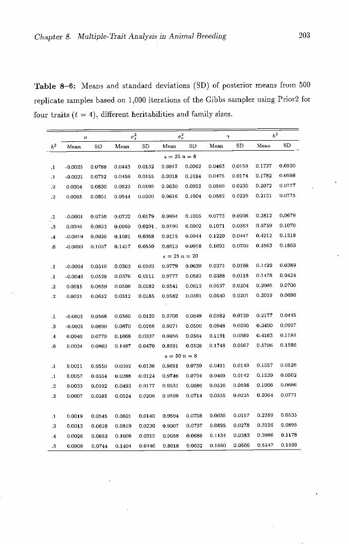
Chapter 8. Multiple-Trait Analysis in Animal Breeding 203
Table 8-6: Means and standard deviations (SD) of posterior means from 500
replicate samples based on 1,000 iterations of the Gibbs sampler using Prior2 for
four traits (t = 4), different heritabilities and family sizes.
/2 cr
it 2 Mean SD Mean SD Mean SD Mean SD Mean SD
s = 25n = 8
.1 -0.0025 0.0788 0.0443 0.0132 0.9817 0.0962 0.0463 0.0153 0.1737 0.0530
.1 -0.0031 0.0752 0.0459 0.0155 0.9918 0.1014 0.0475 0.0174 0.1782 0.0598
.2 0.0004 0.0830 0.0523 0.0195 0.9630 0.0952 0.0560 0.0230 0.2072 0.0777
.2 0.0065 0.0851 0.0544 0.0200 0.9616 0.1004 0.0582 0.0229 0.2151 0.0775
0.0179
0.0291
0.0368
0.0550
0.0103
0.0111
0.0182
0.0185
0.0120
0.0256
0.0337
0.0470
0.0136
0.0124
0.0177
0.0206
1 -0.0001 0.0756 0.0732
3 0.0046 0.0852 0.0959
4 -0.0019 0.0926 0.1081
6 -0.0093 0.1057 0.1417
1 -0.0004 0.0516 0.0363
1 -0.0043 0.0529 0.0376
2 0.0015 0.0659 0.0506
2 0.0021 0.0652 0.0512
1 -0.0031 0.0568 0.0560
3 -0.0031 0.0699 0.0870
4 0.0040 0.0779 0.1068
6 0.0034 0.0863 0.1487
1 0.0011 0.0550 0.0392
1 0.0057 0.0554 0.0388
2 0.0033 0.0592 0.0493
2 0.0007 0.0585 0.0524
0.9694 0.1005
0.9190 0.0902
0.9115 0.0944
0.8613 0.0918
s = 25 n = 20
0.9779 0.0639
0.9777 0.0582
0.9541 0.0612
0.9582 0.0591
0.9706 0.0648
0.9271 0.0590
0.9056 0.0564
0.8591 0.0538
a = 50 n = 8
0.9691 0.0739
0.9746 0.0704
0.9531 0.0686
0.9598 0.0714
0.0773 0.0208 0.2812 0.0679
0.1071 0.0353 0.3759 0.1070
0.1220 0.0447 0.4212 0.1318
0.1695 0.0700 0.5563 0.1863
0.0375 0.0108 0.1429 0.0389
0.0388 0.0118 0.1478 0.0424
0.0537 0.0204 0.2005 0.0706
0.0540 0.0201 0.2019 0.0696
0.0582 0.0129 0.2177 0.0445
0.0948 0.0290 0.3400 0.0927
0.1191 0.0389 0.4163 0.1185
0.1748 0.0567 0.5796 0.1586
0.0411 0.0149 0.1557 0.0526
0.0405 0.0142 0.1539 0.0502
0.0526 0.0198 0.1966 0.0686
0.0555 0.0225 0.2064 0.0771
.1 0.0019 0.0545 0.0601 0.0140 0.9594 0.0708 0.0635 0.0157 0.2359 0.0535
.3 0.0013 0.0628 0.0819 0.0236 0.9307 0.0737 0.0895 0.0278 0.3226 0.0895
.4 0.0026 0.0653 0.1008 0.0315 0.9058 0.0688 0.1134 0.0383 0.3986 0.1178
.5 0.0009 0.0744 0.1404 0.0446 0.8618 0.0632 0.1660 0.0566 0.5547 0.1599
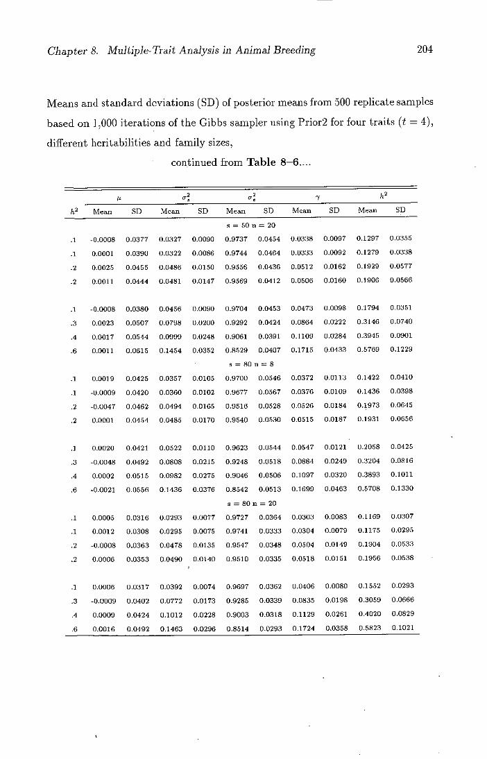
Chapter 8. Multiple-Trait Analysis in Animal Breeding 204
Means and standard deviations (SD) of posterior means from 500 replicate samples
based on 1,000 iterations of the Gibbs sampler using Prior2 for four traits (t = 4),
different heritabilities and family sizes,
continued from Table 8-6....
IL -y h2 Mean SD Mean SD Mean SD Mean SD Mean 5D
s = 50 a = 20
.1 -0.0008 0.0377 0.0327 0.0090 0.9737 0.0454 0.0338 0.0097 0.1297 0.0355
.1 0.0001 0.0390 0.0322 0.0086 0.9744 0.0464 0.0333 0.0092 0.1279 0.0338
.2 0.0025 0.0455 0.0486 0.0150 0.9556 0.0436 0.0512 0.0162 0.1929 0.0577
.2 0.0011 0.0444 0.0481 0.0147 0.9569 0.0412 0.0506 0.0160 0.1906 0.0566
0.0090
0.0200
0.0248
0.0352
0 .0 10 5
0.0102
0.0165
0.0170
1 -0.0008 0.0380 0.0456
3 0.0023 0.0507 0.0798
4 0.0017 0.0544 0.0999
6 0.0011 0.0615 0.1454
1 0.0019 0.0425 0.0357
1 -0.0009 0.0420 0.0360
2 -0.0047 0.0462 0.0494
2 0.0001 0.0454 0.0485
0.9704 0.0453
0.9292 0.0424
0.9061 0.0391
0.8529 0.0407
S = 80 n = 8
0.9700 0.0546
0.9677 0.0567
0.9516 0.0528
0.9540 0.0530
0.0473 0.0098 0.1794 0.0351
0.0864 0.0222 0.3146 0.0740
0.1109 0.0284 0.3945 0.0901
0.1715 0.0433 0.5769 0.1229
0.0372 0.0113 0.1422 0.0410
0.0376 0.0109 0.1436 0.0398
0.0526 0.0184 0.1973 0.0645
0.0515 0.0187 0.1931 0065€
.1 0.0020 0.0421 0.0522 0.0110 0.9623 0.0544 0.0547 0.0121 0.2058 0.0425
.3 -0.0048 0.0492 0.0808 0.0215 0.9248 0.0518 0.0884 0.0249 0.3204 0.0816
.4 0.0002 0.0515 0.0982 0.0275 0.9046 0.0506 0.1097 0.0320 0.3893 0.1011
.6 -0.0021 0.0556 0.1436 0.0376 0.8542 0.0513 0.1699 0.0463 0.5708 0.1330
s = 8011 = 20
.1 0.0005 0.0316 0.0293 0.0077 0.9727 0.0364 0.0303 0.0083 0.1169 0.0307
.1 0.0012 0.0308 0.0295 0.0075 0.9741 0.0333 0.0304 0.0079 0.1175 0.0295
.2 -0.0008 0.0363 0.0478 0.0135 0.9547 0.0348 0.0504 0.0149 0.1904 0.0533
.2 0.0006 0.0353 0.0490 0.0140 0.9510 0.0335 0.0518 0.0151 0.1956 0.0538
.1 0.0006 0.0317 0.0392 0.0074 0.9697 0.0362 0.0406 0.0080 0.1552 0.0293
.3 -0.0009 0.0402 0.0772 0.0173 0.9285 0.0339 0.0835 0.0198 0.3059 0.0666
.4 0.0009 0.0424 0.1012 0.0228 0.9003 0.0318 0.1129 0.0261 0.4020 0.0829
.6 0.0016 0.0492 0.1463 0.0296 0.8514 0.0293 0.1724 0.0358 0.5823 01021
V

Chapter 8. Multiple-Trait Analysis in Animal Breeding 205
Table 8-7: Means and standard deviations (SD) of ANOVA estimates and poste-
rior expectations, based on 1,000 Gibbs sampling using two different priors (Priori
and Prior2), of canonical heritabilities (A) from 500 replicate samples for four traits
(t = 4), different heritabilities and family sizes.
ANOVA Priori Prior2
h2 Mean SD Mean SD Mean SD
s = 25n = 8
.1 -0.1931 0.0955 0.0487 0.0075 0.0558 0.0069
.1 0.0124 0.1138 0.0985 0.0137 0.1038 0.0137
.2 0.2358 0.1282 0.1975 0.0365 0.1955 0.0359
.2 0.5389 0.1820 0.4409 0.1093 0.4225 0.1027
1 -0.1095 0.1197
3 0.1512 0.1425
4 0.4496 0.1761
6 0.8624 0.2113
1 -0.0335 0.0460
1 0.0712 0.0555
2 0.1875 0.0687
2 0.3583 0.0978
1 0.0215 0.0634
3 0.1982 0.0885
4 0.4132 0.1154
6 0.7350 0.1676
1 -0.1011 0.0780
1 0.0544 0.0803
2 0.2109 0.0902
2 0.4126 0.1143
0.0708 0.0159
0.1973 0.0322
0.3980 0.0686
0.7574 0.0936
s = 25 n = 20
0.0502 0.0071
0.0953 0.0154
0.1813 0.0342
0.3555 0.0762
0.0726 0.0170
0.2159 0.0437
0.4130 0.0735
0.7298 0.0997
S = 50 n = 8
0.0494 0.0070
0.0945 0.0140
0.1821 0.0341
0.3718 0.0829
0.1298 0.0179
0.2377 0.0330
0.4309 0.0790
0.8250 0.1748
0.0583 0.0069
0.1019 0.0152
0.1799 0.0330
0.3497 0.0759
0.1304 0.0173
0.2379 0.0390
0.4168 0.0733
0.7506 0.1370
0.0571 0.0067
0.1012 0.0138
0.1836 0.0337
0.3711 0.0880
.1 -0.0213 0.0972 0.0759 0.0172 0.1278 0.0168
.3 0.2056 0.1078 0.2136 0.0424 0.2333 0.0381
.4 0.4326 0.1159 0.4129 0.0772 0.4106 0.0739
.6 0.7438 0.1553 0.7527 0.1314 0.7321 0.1319
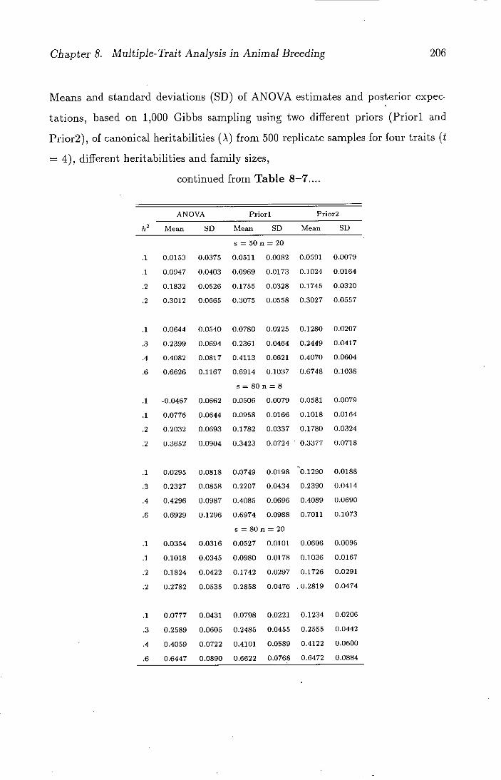
Chapter S. Multiple-Trait Analysis in Animal Breeding 206
Means and standard deviations (SD) of ANOVA estimates and posterior expec-
tations, based on 1,000 Gibbs sampling using two different priors (Priori and
Prior2), of canonical heritabilities (A) from 500 replicate samples for four traits (t
= 4), different heritabilities and family sizes,
continued from Table 8-7....
ANOVA Priori Prior2
h2 Mean SD Mean SD Mean SD
s = 50n= 20
.1 0.0153 0.0375 0.0511 0.0082 0.0591 0.0079
.1 0.0947 0.0403 0.0969 0.0173 0.1024 0.0164
.2 0.1832 0.0526 0.1755 0.0328 0.1745 0.0320
.2 0.3012 0.0665 0.3075 0.0558 0.3027 0.0557
1 0.0644 0.0540
3 0.2399 0.0694
4 0.4082 0.0817
6 0.6626 0.1167
1 -0.0467 0.0662
1 0.0776 0.0644
2 0.2032 0.0693
2 0.3652 0.0904
1 0.0295 0.0818
3 0.2327 0.0858
4 0.4296 0.0987
6 0.6929 0.1296
1 0.0354 0.0316
1 0.1018 0.0345
2 0.1824 0.0422
2 0.2782 0.0535
0.0780 0.0225
0.2361 0.0464
0.4113 0.0621
0.6914 0.1037
S = 80 n = 8
0.0506 0.0079
0.0958 0.0166
0.1782 0.0337
0.3423 0.0724
0.0749 0.0198
0.2207 0.0434
0.4085 0.0696
0.6974 0.0988
s = 80n = 20
0.0527 0.0101
0.0980 0.0178
0.1742 0.0297
0.2858 0.0476
0.1280 0.0207
0.2449 0.0417
0.4070 0.0604
0.6748 0.1038
0.0581 0.0079
0.1018 0.0164
0.1780 0.0324
0.3377 0.0718
0.1290 0.0188
0.2390 0.0414
0.4089 0.0690
0.7011 0.1073
0.0606 0.0095
0.1036 0.0167
0.1726 0.0291
0.2819 0.0474
.1 0.0777 0.0431 0.0798 0.0221 0.1234 0.0206
.3 0.2589 0.0605 0.2485 0.0455 0.2555 0.0442
.4 0.4059 0.0722 0.4101 0.0589 0.4122 0.0600
.6 0.6447 0.0890 0.6622 0.0768 0.6472 0.0884

Chapter 9
Multiple-Trait Selection Indices
9.1 Introduction
In the development of animal breeding plans it is common practice to consider
several traits. These traits may differ in heritability, economic importance and
phenotypic variance. The following question arises in what way shall the breed-
ing animals be selected to improve several traits genetically? The principal of
constructing and using selection indexes which permit attainment of maximum
genetic progress for several traits in animal breeding situations was originally pro-
posed by Hazel (1943). The theory was considered in somewhat greater depth
by Henderson (1963) who combined information from several individuals for one
or more traits. The paper by Hazel (1943) introduced the formalized theory of
selection index into animal breeding as Smith (1936) did for plant breeding. The
primary idea presented by Hazel (1943) was certainly not focused on the use of
different sources of information for single-trait evaluations; rather it emphasized
the definition of multiple-trait breeding goals and objective means of assessing
appropriate weights to the different traits being recorded, considering genetic re-
lationships and variances and covariances among the traits included.
Williams (1962a) obtained an exact formula for the sampling variance of the
index weights for two variables in a specific experimental design with selection
applied to groups rather than individuals. These particular sampling and selec-
207

Chapter 9. Multiple-Trait Selection Indices 208
tion schemes were chosen to reduce the problem to one that was mathematically
tractable. He suggested the use of a base index, in which the economic weights
are used directly as the index weights, instead of the index computed from the
estimated parameters. He showed that progress from using the estimated index
for two traits could be substantially smaller than that from using the base index.
Williams (1962b) has suggested that unless a considerable amount of data was
available for parameter estimation, it would be preferable to select upon the base
index than upon an estimated index. His conclusion was that if the improvement
of the optimum over the base index is small, then the chance of achieving an even
smaller improvement over the base index with the estimated index may not be
large enough to outweigh the risk that the estimates provide results worse than
those for the base index.
Harris (1964) considered the nature of the index selection procedure when
sample estimates are used in place of true parameter values. He adopted a rather
different approach, using Taylor series expansions to develop approximate formulae
for the expected achieved response from paternal half-sib analyses of variance
and covariance. These formulae were complicated, although only two traits with
individual selection were considered. The validity of the results was checked by
Monte Carlo simulation and was supported fairly strongly.
According to Hazel and Lush (1942) multiple-trait selection can be carried out
by three main methods. They are as follows
The tandem method,i.e. select for one trait until that is improved, then for a
second trait, later for a third, etc., until finally each trait has been improved to
the desired level.
The independent culling levels, i.e. a certain level of merit is established for
each trait, and all individuals below that level are discarded, regardless of the
superiority or inferiority of their other traits.
The selection index method, i.e. select for all the traits simultaneously by using

Chapter 9. Multiple-Trait Selection Indices 209
some index of net merit constructed by adding into one figure the credits and
penalties given each animal according to the degree of its superiority or inferiority
in each trait.
If the parameters were known or estimates of them exist the selection in-
dex method should be preferred. Since the introduction of the selection index
method by Hazel (1943), it has been considered the best method, theoretically,
for multiple-trait improvement. It has several theoretical advantages when the
joint distribution of breeding values and traits is known; minimizing the predic-
tion error, maximizing the correlation between true breeding value and the pre-
dicted value, maximizing the probability of correct ranking, and maximizing the
average true breeding value of a selected group of individuals. It has also been
shown (Hazel and Lush, 1942) that the index method is never less efficient than
that of independent culling levels, though it might be no more efficient; similarly,
independent culling is never less efficient than tandem selection.
However, when selection of individuals for two or more traits must be per-
formed, the mean, variances and covariances are required to be known, and the
genetic and phenotypic values to be normally distributed. Despite the fact that
these assumptions are satisfactory for continuous type of traits, e.g. milk yield,
protein yield, fat yield and growth rate, some selection experiments have failed
to demonstrate the superiority of index selection over independent culling levels.
The failure of the index method of selection to achieve expectations may be due
to invalid assumptions (Xu and Muir, 1990).
The problems with the selection index approach is that if the variance matrix
of explanatory variables is ill-conditioned, i.e., the eigenvalues of the matrix are
spread and some of them are very small (approximately zero), the least square
estimates of the regression coefficients are much more sensitive to sampling er-
rors. The bending method developed by Hayes and Hill (1981) and outlined in
Chapter 8 for variance matrices can be used to reduce the problem of sampling

Chapter 9. Multiple-Trait Selection Indices 210
errors. In order to circumvent the problem of an ill-conditioned covariance matrix
of explanatory variables in multiple regression analysis, the technique of ridge re-
gression was introduced by Hoerl and Kennard (1970) to obtain a class of biased
estimators for the parameters in a general linear model. The bending procedure
has its roots in this technique.
In recent years, there have been several other studies that have investigated
a method of modifying (bending) the parameter estimates so as to improve the
selection responses for several traits. Meyer and Hill (1983) developed a more
general bending procedure which can be applied to any combination of traits,
when both individual and sib information are available. Since they found that it
improved poor indices much more than it worsened good indices, it can be used
with some safety. The choice of the bending factor was problematical, but Monte
Carlo simulation suggested that at least some bending could be done to advantage
in all situations (like Hayes and Hill, 1981).
In contrast to Hayes and Hill (1981), Hayes and Cue (1985) dealt with estimates
of variances and covariances for two and three traits from unbalanced data sets.
They considered two methods of estimation, a) Restricted Maximum Likelihood
(Thompson, 1973), and b) Henderson's method III (Henderson, 1953). Their
objective was to see if these estimates can be improved by bending and to what
extent in the case of each method. In all cases the achieved response was improved
by bending. The improvement in the achieved response was greater in the case of
three traits than two traits.
Meuwissen and Kanis (1988) used a bending procedure in combination with
the general consistency criterion of Foulley and 011ivier (1986) to modify an in-
consistent set of guessed population parameters in a pig breeding situation where
many index traits and a few breeding goal traits are involved.
A new method for the choice of an appropriate bending factor in the con-
struction of genetic selection indices using some prior knowledge of the population
Chapter 9. Multiple-Trait Selection Indices 211
parameters was developed by Essi (1991). The main feature of the method that
he proposed is to use the bending factor which maximizes the correlation between
true and estimated aggregate genotype, replacing the (unknown) population pa-
rameters with guessed values in the computation formula.
The general use of decision theory in determining selection procedures and
the application of the theory for a single trait using data on candidates and their
relatives are given in Chapter 7. The extension of the method to multiple trait
individual selection will be examined with simulated data sets in this chapter.
Theoretical assessment of selection progress from a Bayesian decision procedure
point of view is carried out by Theobald (1994) for a single trait and multiple trait
selections but no numerical results are presented.
In this chapter, a balanced multiple trait one-way sire model is considered
for selection of a fixed proportion from an infinite population. The conventional
method of constructing genetic selection indices for multiple traits is reviewed and
the use of the bending method for improving selection responses is considered.
Then Bayesian decision procedures are contrasted with the use of conventional
and modified estimates. Bayesian inferences about the selection responses are
made from the marginal posterior distributions which are obtained using the Gibbs
sampling algorithm described in Chapter 8 for multiple trait analysis.
9.2 Theory of Multiple Trait Index Selection
Let us assume that t traits are observed, and let x and g denote the vector of
observations on an individual and the corresponding vector of additive genetic
contributions. The aggregate breeding value of the individual, which is determined
jointly by the breeding values and the economic importance of the component
traits is given by
H = ag,

Chapter 9. Multiple-Trait Selection Indices 212
where a is a vector of relative economic weights corresponding to g. The economic
weight for each trait should approximate the partial regression of cost per unit of
enterprise output value on the corresponding breeding value. These weights can
vary with the production and marketing system, with performance of traits, and
with breed role (i.e., paternal, maternal, or general) in crossbreeding systems.
Since the value of H for a particular individual will not be known, selection
is carried out on an index, I, thought to be positively correlated with H. An
index intended to maximize the correlation with aggregate breeding value H is
then constructed as follows
I=b'x
(9.1)
where b is a vector of index weights. Genetic improvement in H is proportional
to PHI, the correlation between index values and aggregate breeding value, which
is given by a'E9 b
PHI =
where E and E. are the phenotypic and genetic variance matrices between traits.
It is well-known that PHI has a maximum when b equals to
= E; 1 E9 a. (9.2)
The response, II, to selection is then
= 1Cov (I , H)[Var(I)]_h/'2
=
= (a'E9E1ga)1/2, (9.3)
where i is the selection intensity or average superiority of the index. The popula-
tion parameters L and )i g are assumed to be known without errors in the index

Chapter 9. Multiple-Trait Selection Indices
213
weight and response calculations. However, this is not likely to be the case in
practice.
If the index is computed from estimates of parameters, more quantities need
to be defined (Sales and Hill, 1976). Given estimates E,, and )i of E and E.,
the estimated index weights are usually taken from (9.2) as
= EE9 a
(9.4)
with the economic weights assumed to be known without error. The predicted
response, R, is calculated by substituting the estimates into (9.3) as follows
=
1/2 = 9 a) . (9.5)
The expectation of the response that is actually achieved using estimated weights,
to make selection decisions in the population is
= i Cov(I,H)[Var(i)] -'12
- ibE9 a (9.6)
- (6'E6)1/2
9.2.1 The Bending method
Instead of using either the index computed from the parameter estimates directly,
or simply the base index, it is possible to construct selection indices using modified
parameter estimates. One method, termed bending, was proposed by Hayes and
Hill (1981) and is outlined in Section 8.2.3.
The modified estimated and achieved responses can be obtained as
ir =

Chapter 9. Multiple-Trait Selection Indices 214
fro= ib Ea
(6*'EpU) £*\1/2
*-1* where the bent estimate b is obtained as b * = E 7, E9 a.
When w = 1, b = E - 'Ea = ca where c = 4( - 1)/(U + n - 1), w is a
bending factor and v is the mean of the roots of MMb and when w = 0,
9.3 Negative Roots and Their Modification
9.3.1 Negative Roots (Heritabilities)
In the analysis of correlated traits there is a strong chance that because of sampling
variation, the estimated variance matrix of genetic components, FIg, is not positive
definite. The probability that this occurs increases with the number of traits (Hill
and Thompson, 1978). The use of estimated variance matrices obtained from
using ANOVA can cause some problems.
Firstly, if there are many traits, the estimates Ak of roots Ak obtained from
the determinantal equation I Eg - XE7, 1= 0 may be seriously biased (Hill and
Thompson, 1978). This is illustrated using a canonical transformation of ANOVA
estimates, Eg and EP, for four traits in Table 8-7 of Chapter 8. In this table,
the estimates of high values of Ak are biased upwards and of low values are biased
downwards as also reported by Hayes and Hill (1980). The biases are greatest
when the parameter values, Ak, are close together. It appears that the biases
decrease with an increase in the family size.
Secondly, one or more roots of E; 1 E9 calculated from the ANOVA method are
likely to be negative, especially when there are many traits. The negative roots
mean that there are sets of economic weights for which index selection would
give negative progress. This can be seen from Table 8-7 in Chapter 8. The

Chapter 9. Multiple-Trait Selection Indices 215
negative roots in this table are generally of small magnitude, but problems might
be expected if these become large relative to the dominating positive roots. The
use of such estimates in the construction of selection indices may lead to inefficient
selection decisions even when data on hundreds of animals are used.
However the use of posterior expectations of genetic and phenotypic variance
matrices; and E obtained from Gibbs sampling estimates overcomes the prob-
lems mentioned above which are encountered using ANOVA estimates.
As a first check on whether the estimated parameters are within the permissi-
ble parameter space one might look at the estimated canonical heritabilities, that
is the estimated heritabilities of the canonical variables, which are the roots 'k, of
E 1 E9 , i.e., solutions of J - 0. If any of these are less than zero they
imply negative genetic variances for the corresponding canonical variables, equiv-
alent to untransformed heritabilities or genetic correlations outside their bounds.
A solution of Ak of I E,, - 0 is negative if and only if Y has a negative
eigenvalue. If any of the A, exceed unity they imply negative environmental cor-
relations exceeding unity in absolute value for the canonical variables (necessary
and sufficient condition that I E, - 0 has at least one A, > 1 is that
EP -; = E e has at least one negative eigenvahie).
9.3.2 Possible modifications of negative roots
It is obvious that estimates are faulty if the canonical heritabilities fall outside
their bounds, but how to deal with the unreasonable estimates remains an open
question. When estimated correlations and/or heritabihties have been outside
their bounds, it has been the common practice in simulation studies to set them
to the nearest valid bound, for example negative heritabilities to zero, correlations
over unity to one (Harris, 1964; Sales and Hill, 1976, 1977). This is equivalent to
setting a canonical heritability to its nearest bound, either 0 or 1.
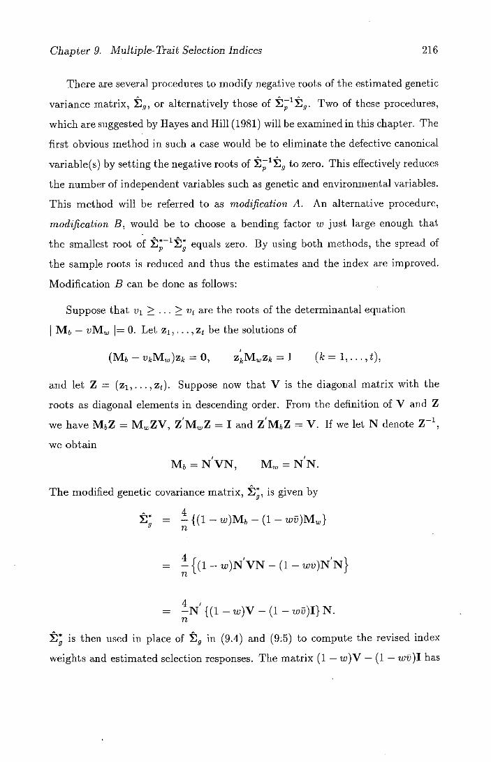
Chapter 9. Multiple-Trait Selection Indices 216
There are several procedures to modify negative roots of the estimated genetic
variance matrix, E 9 , or alternatively those of 1 Jg . Two of these procedures,
which are suggested by Hayes and Hill (1981) will be examined in this chapter. The
first obvious method in such a case would be to eliminate the defective canonical
variable(s) by setting the negative roots of t P 1 t g to zero. This effectively reduces
the number of independent variables such as genetic and environmental variables.
This method will be referred to as modification A. An alternative procedure,
modification B, would be to choose a bending factor w just large enough that
the smallest root of E 1 equals zero. By using both methods, the spread of
the sample roots is reduced and thus the estimates and the index are improved.
Modification B can be done as follows:
Suppose that v 1 > ... > Vt are the roots of the determinantal equation
I M - VM =0. Let z l ,..., zt be the solutions of
(Mb —VkM)Zk = 0, z kMwzk = 1 (k=
and let Z = (z i ,. . . , z t ). Suppose now that V is the diagonal matrix with the
roots as diagonal elements in descending order. From the definition of V and Z
we have M5Z = MWZV, Z'MW Z = I and IMbZ = V. If we let N denote Z',
we obtain
M6 =NVN, M=NN.
The modified genetic covariance matrix, E, is given by
= {(1—w)Mb—(l—wU)M}
= {(i - w)N'VN - (1 - wU)N'N}
= ±N'{(l — w)V — (1 —wU)I}N.
is then used in place of E9 in (9.4) and (9L5) to compute the revised index
weights and estimated selection responses. The matrix (1 - w)V - (1 - wU)I has

Chapter 9. Multiple-Trait Selection Indices 217
diagonal elements (1, — w)vk - (1 - w13). The smallest of them is
(1 - W)Vt - ( 1 - wD) = Vt - 1 - W(Vt - ü).
This is non-negative if Vt - 1 > W(vt - ü), or
1 - Vt
V - Vt
Thus, one should choose a bending factor (1 - V1)/(v - Vt) in order to make
non-positive definite.
9.4 A Decision Theory Approach
A general decision theory approach to selection of candidates for breeding is al-
ready discussed in Chapter 7. In what follows this approach will be extended
briefly to multiple-trait selection procedures.
Suppose that the data vector x oft traits is recorded on an individual candidate
for selection and that Y denotes the experimental observations of the some traits
on other members of the same population. Genetic theory postulates a vector g of
genetic values representing the expected values of these traits among progeny from
mating this individual in a specified population. Suppose, for simplicity, that the
proportion of candidates to be selected is fixed. We might then take the utility of
selecting a particular candidate to be its aggregate breeding value a'g. The best
animals are then those for which the posterior expectation of the breeding value
is greatest. Hence we require the posterior expectation of a'g, and the preferred
candidates are those maximizing
E[a'E g E'x I P,Y] = a'E[B I P,Y]x, (9.7)
where F denotes the prior distribution on ji, E, , and E and B is the posterior
expectation of E9 E;'. Expression (9.7) still represents a linear index in x, but
the coefficients in B are obtained as posterior expectations, not via estimation.
The Gibbs sampler allows these expectations to be found straightforwardly.

Chapter 9. Multiple-Trait Selection Indices 218
9.5 Results From 500 Replicate Samples of Sim-
ulation Study
9.5.1 Data
Observations generated using a balanced multiple trait one-way sire model in (8.1)
of Chapter 8 are also employed here to assess selection progress. Values Yij for half-
sib groups were generated for various numbers of sires, family sizes, heritabilities
and numbers of traits In all simulations, 500 replicate data sets were used and
results for selection responses from ANOVA estimates and posterior expectations
of the parameters are based on averages over these replicates for each experimental
design.
9.5.2 Results
Results from conventional selection procedures: The optimum selection responses,
R02 , for given heritabilities, economic weights and number of traits (t = 2, 4
and 6) are illustrated in Table 9-1. Means and standard deviations of estimated
response Rand of achieved response if using ANOVA estimates from 500 replicate
samples for a range of traits, different heritabilities, economic weights, family sizes
and bending factor, w, are shown in Tables 9-2 and 9-3, respectively. Estimates
falling outside the parameter space were not excluded from the analysis, i.e., roots
of E' E9 could be outside the range 0 to 1, including cases of negative heritability
estimates. As in the case of a single trait selection indices, comparison of the
values of Table 9-2 with those of Table 9-1 indicates that the estimated responses
R almost always overestimate the optimum progress R, pt . This upwards bias is
considerable especially when there are a few families and many traits but becomes
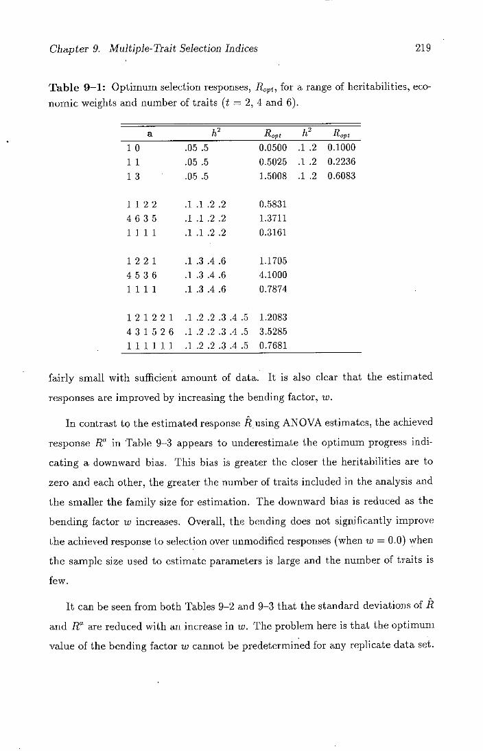
Chapter 9. Multiple-Trait Selection Indices 219
Table 9-1: Optimum selection responses, for a range of heritahilities, eco-
nomic weights and number of traits (t = 2, 4 and 6).
2 U a It Ibopt 1.
-'1opt
1 0 .05 .5 0.0500 .1 .2 0.1000
11 .05 .5 0.5025 .1 .2 0.2236
1 3 .05 .5 1.5008 .1 .2 0.6083
1122 .1.1.2.2 0.5831
4635 .1.1.2.2 1.3711
11 1 1 .1 .1 .2 .2 0.3161
1221 .1.3.4.6 1.1705
4536 .1.3.4.6 4.1000
1 1 1 1 .1 .3 .4 .6 0.7874
12 122 1 .1.2.2.3.4.5 1.2083
431526 .1.2.2.3.4.5 3.5285
111111 .1.2.2.3.4.5 0.7681
fairly small with sufficient amount of data. It is also clear that the estimated
responses are improved by increasing the bending factor, w.
In contrast to the estimated response Eusing ANOVA estimates, the achieved
response H" in Table 9-3 appears to underestimate the optimum progress indi-
cating a downward bias. This bias is greater the closer the heritabilities are to
zero and each other, the greater the number of traits included in the analysis and
the smaller the family size for estimation. The downward bias is reduced as the
bending factor in increases. Overall, the bending does not significantly improve
the achieved response to selection over unmodified responses (when w = 0.0) when
the sample size used to estimate parameters is large and the number of traits is
few.
It can be seen from both Tables 9-2 and 9-3 that the standard deviations of I?
and H" are reduced with an increase in in. The problem here is that the optimum
value of the bending factor w cannot be predetermined for any replicate data set.
Chapter 9. Multiple-Trait Selection Indices
220
Table 9-2: Means and standard deviations (SD) of estimated response to selec-
tion, .ñ, using ANOVA estimates from 500 replicate samples for a range of traits (t
= 2, 4 and 6), different heritabilities, economic weights, family sizes and bending
factor, W.
0.0 0.2 0.4 0.6 018
0 Mean SD Mean a
SD Mean SD Mean SD Mean SD
S = 25. =8
1 0 .05 .5 0.1972 0.1160 0.1815 0.1152 0,1947 0.1206 0.2248 0,1326 0.2657 0.1509
1 1 .05 .5 0.5595 0,2937 0.5097 0.2723 0.4700 0.2545 0,4425 0.2410 0,4285 0.2337
1 3 .05 .5 1.5925 0,7899 1.4464 0.7254 1.3045 0.6629 1,1687 0.6032 1,0418 0.5486
1 0 .1 .2 0.2109 0,1261 0,1912 0.1178 0.1763 0.1129 0.1671 0.1117 0,1646 0.1144
1 3 .3 .2 0.3416 0,1994 0,3095 0.1851 0.2816 0.1746 0.2592 0.1685 0,2443 0.1666
1 3 .1 .2 0,8263 0,4766 0.7469 0.4434 0.6746 0,4157 0,6118 0.3946 0,5619 0,3812
1 3 2 2 .1 .1 .2 .2 1,0144 0.4723 .0.8772 0,4259 0,7537 0,3838 0,6515 0.3415 0,5795 0.3120
4 6 5 3 .3 .1 .2 .2 2.8265 3,3281 2.4353 1.1890 2,0952 1,0586 1.8282 0,9514 1,6581 0,8969
1 1 1 1 .1 .1 .2 .2 0,6182 0,2896 0.5334 0,2603 0,4588 0,2327 0,3991 0.2092 0,3597 0,1953
1 2 2 1 .1 .3 .4 .6 1.4805 0.6028 1,3664 0,5452 1,2810 0,4865 1,2261 0,4363 1,2020 0,4083
4 5 3 6 .1 .3 .4 .6 4,8866 2.0113 4,4513 1,7999 4,0855 3.5826 3,8008 1,3807 3,6071 1.2350
1 1 1 1 .1 .3 .4 .6 0,9725 0.4001 0,8889 , 0,3611 0,8254 0.3204 0,7830 0,2838 0,7624 0,2607
1 2 1 2 2 1 .2 .2 .2 .3 .4 .5 1,8023 0.6691 1.5948 0.6045 1,4246 0.5303 1,3028 0,4501 1,2346 0.3901
4 3 1 5 2 6 .2 .2 .2 .3 .4 .5 4,8566 3,7277 4,2948 1,5375 3,8025 1,3345 3,4044 3,3318 3,1254 0.9779
1 1 1 1 3 1 .1 .2 .2 .3 .4 .5 1,0435 0,4298 1,0097 0,3877 0,9007 0.3382 0,8225 0.2868 0,1794 0,2492
a = 25 n = 20
1 0 .05 .5 0.1001 0,0605 0,1204 0,0629 0.2583 0,0680 0.2023 0,0781 . 0,2486 0.0920
1 I .05 .5 0.5007 0,1900 0,4642 . 0.1149 0,4353 0,1619 0.4253 0,1519 0,4052 0.1464
1 3 .05 .5 1.4897 0,5265 1,3621 0,4818 2.2365 0,4374 1,1337 0,3943 0.9952 0,3533
1 0 .2 .2 0.1299 0,0696 0,1303 0,0654 013345 0,0619 0,1413 0,0610 0.1503 0,0630
1 2 .1 .2 0.2507 0,1321 0,2398 0,1209 0.2322 0,1102 0,2274 0,1015 0.2254 0,0962
1 3 .1 .2 0,6775 0,3393 0,6356 0,3085 0,5967 0,2790 0,5813 0,2518 015299 0,2263
1 I 2 2 .1 .1 .2 .2 0.7060 0,3072 0,6427 0,2719 0,5872 0,2354 0,5407 0,2007 0,3046 0,1729
4 6 3 3 .1 .1 .2 .2 1,7828 0,7780 1,6331 0.6988 1,5180 0,6166 1,4424 0,5390 3,4077 0,4836
1 3 1 1 .1 .1 .2 .2 0.3998 0,1745 0,3658 0,3558 0,3385 0,1365 0,3189 0,1186 0,3075 0.1054
1 2 2 1 .1 .3 .4 .6 1.3118 0.4951 1.2530 0.4298 1.2079 0.3660 1,1766 0,3109 1.1593 0,2748
4 5 3 6 .1 .3 .4 .6 4.4770 1,5187 4,1650 1,3262 3.8911 3,3364 3.6639 0.9645 3,4849 0.8360
1 2 2 1 .1 .3 .4 .6 0.8744 0,3087 0,8229 0,2694 0.7821 0,2307 0,7528 0.3971 0.7357 0,3748
1 2 1 2 2 1 .1 .2 .2 .3 .4 .5 1.4335 0,4950 1,3307 0,4295 112474 0,3608 1,1858 0,2950 1,1477 0,2457
4 3 3 3 2 6 .1 .2 .2 .3 .4 .5 4.0367 1,3629 3,6873 1,1775 3.3768 0,9814 3.1349 0,7905 2.9093 0,6371
1 2 2 1 1 1 .1 .2 .2 .3 .4 .5 0.9112 0,3060 0,8438 0,2671 0.7863 0,2257 0.7463 0,3859 0,7234 0,1562
= 50 n = 8
1 0 .05 .5 0,2377 0.0764 0,1436 0,0819 0.1677 0,0893 0.2071 0,0974 0,2519 0.1084
1 1 .05 .5 0,5202 0.2352 0,4808 0,1973 0.4489 0,1823 0,4260 0,1716 0,4331 0,1664
1 3 .05 .5 3.5209 0,5730 3,3893 0,5246 1.2597 0,4779 1,2334 0,4338 1.0119 0.3942
1 0 .1 .2 0,1353 0.0888 0,1466 0,0863 0,2429 0,0845 0,1448 0,0831 0,1512 0,0836
1 1 .1 .2 0,2814 0.1532 0,2620 0,1428 0,2464 0,1335 0,2351 0,1258 0.2282 0.1213
1 3 .1 .2 0,7275 0,3657 0,6720 0.3383 0,6206 0.3339 0.5742 0.2939 0,5342 0.2790
1 1 2 2 .1 .1 .2 .2 0,8065 0,3369 0,7162 0,3002 0,6351 0,2662 0,5671 0,2373 0,5188 0,2175
4 6 5 3 .1 .1 .2 .2 2,0800 0,9116 1,8463 0,8182 1,6544 0,7303 1,5157 0.6611 1,4432 0,6239
1 1 1 2 .1 .1 .2 .2 0.4682 0.2041 0.4355 0.1825 0.3708 0.1626 0.3366 0.1461 0.3160 0.1357
1 2 2 1 .1 .3 .4 .6 1.3087 0.4759 1.2429 0.4189 1.1948 0.3611 1,1645 0.3097 1.1514 0.2756
4 5 3 6 .1 .3 .4 .6 4,4467 1.5424 4.3248 1.3493 3.8501 1.1507 3.6281 0,9667 3.4649 0.8302
1 1 3 1 .1 .3 .4 .6 0,8741 0,3138 0.8186 0.2759 0.7760 0.2369 0.7469 0,2013 0.7317 0.1764
1 2 1 2 2 1 .1 .2 .2 .3 .4 .5 1,5683 0,5667 1.4357 0.5019 3.3283 0.4298 1.2303 0.3553 1.2031 0.2931
4 3 1 5 2 6 .1 .2 .2 .3 .4 .5 4.2748 1,4727 3.8763 1.2942 3,5276 1.1028 3.2419 0.9077 3.0315 0.7389
1 1 1 1 1 1 .1 .2 .2 .3 .4 .5 0,9837 0,3543 0.8980 0.3133 0,8298 0.2680 0.7821 0.2218 0.7562 0,1842

Chapter 9. Multiple-Trait Selection Indices 221
Means and standard deviations (SD) of estimated response to selection, .k, using
ANOVA estimates from 500 replicate samples for a range of traits (t = 2, 4 and
6), different heritabilities, economic weights, family sizes and bending factor, w,
continued from Table 9-2....
0.0 0.2 0,4 0.6 0.8
ah2 Mean SD Mean SD Mean SD Mean SD Mean SD
= 50 n = 20
1 0 .05 .5 010615 0.0423 0.1141 0.0449 0.1582 0.0494 0.2054 0.0574 0.2534 0.0680
1 1 .05 .5 0.5073 0.1382 0.4721 0.1268 0.4440 0.1174 0.4244 0.3108 0.4141 0.1079
1 3 .05 .5 1,5105 0.3975 1.3836 0.3625 1.2582 0,3281 111351 0.2950 1.0156 0.2639
1 0 .1 .2 0.1169 0.0571 0,1205 0.0546 0.1261 0.0524 0.1330 0.0511 0.1409 0.0512
1 1 .1 12 012285 010986 0.2218 0.0910 0.2166 0.0845 0.2129 0.0793 0.2108 0.0760
1 3 .1 .2 0.6011 0,2418 0.5730 0,2224 0,5425 0.2043 0.5158 0,1880 0.4909 0.1749
1 1 2 2 .1 .1 .2 .2 0.6312 0.2158 0,5907 0.1873 0.5547 0.1599 0.5236 0.1360 0.4981 0.1190
4 6 5 3 .1 .1 .2 .2 1.5414 0.5611 1.4692 0.4925 1.4198 0.4263 1.3940 0,3704 1.3916 0.3359
1 1 1 1 .1 .1 .2 .2 0.3511 0.1263 0.3327 0.1103 0.3385 0.0948 0.3090 0,0816 . 0.3041 0.0731
1 2 2 1 .1 .3 .4 .6 1.1939 0.3163 1.1641 0.2725 1.1434 0.2321 1.1319 011998 1.1295 0.1813
4 5 3 6 .1 .3 .4 .6 4.1247 1.0421 3.8915 0,8984 3.6886 0.7603 3.5204 0.6395 3.3918 0.5543
1 1 1 1 .1 .3 .4 .6 0.7951 0.2108 0.7624 0.1813 0,7380 0.1534 0.7223 0.1301 0.7157 0.1159
1 2 1 2 2 1 .1 .2 .2 .3 .4 .5 1.3141 0,3552 1,2504 0,3022 3,1984 0.2492 1,1587 0.2010 1.1324 0.1663
4 3 1 5 2 6 .1 .2 .2 .3 .4 .5 3.7364 0,9381 3.4731 0.7978 3.2364 0.6568 3.0319 0.5253 2.8663 0.4245
1 1 1 1 1 1 .1 .2,2,3,4 .5 0.8311 0.2230 0.7871 0.1898 0.7522 0.1562 0.7272 0.1257 0.7129 0,1044
S = 80 n = 8
1 0 .05 .5 0,1147 0,0627 0,1292 0.0675 0.1632 0.0736 0.2070 0.0796 0,2545 0,0873
1 1 .05 .5 0.5201 0.1713 0.4818 0.1571 0,4509 0.1454 0.4287 0.1369 0.4165 0.1325
1 3 .05 .5 1,5299 0.4548 1.3989 0.4160 1,2695 0.3786 1.1428 0.3435 1.0201 0.3122
1 0 .1 .2 0.1371 0.0770 0.1341 0.0745 0,1352 0.0726 0.1400 0.0717 0.1477 0.0728
1 1 .1 .2 0.2618 0.3320 0.2473 0.1232 0.2359 0.1154 0.2277 0.1093 0.2228 0.1060
1 3 .1 .2 016810 0.3307 0.6360 0.3038 0.5939 0.2796 0.5552 0,2591 0.5207 0.2438
1 1 2 2 .1 .1 .2 .2 0.7341 0.3083 0.6649 0.2742 0.6044 0.2391 0.5546 0,2048 0.5173 0.1767
4 6 5 3 .1 .1 .2 .2 1,9087 0,7757 1,7348 0.7009 1.5957 0,6273 1.5006 0,5564 1.4539 0,5011
1 1 1 1 .1 .1 .2 .2 0,4254 0.1765 0.3881 0,1586 0.3537 0,1409 0.3302 0.1237 0.3067 0,1095
1 2 2 1 .1 .3 .4 .6 1,2554 0,4088 1.2114 0.3583 1.1799 0.3079 1.1605 0.2634 1.1529 0.2329
4 5 3 6 .1 .3 .4 .6 4.2914 1.2026 4.0219 1,0558 3.7892 0.9098 3.5983 0.7775 3.4547 0.6799
1 1 1 1 .1,3,4 .6 0.8352 0.2521 0.7931 012218 0.7613 0.1914 0.7401 0.1645 0.7300 0.1459
1 2 1 2 2 1 .1 .2 .2 .3 .4 .5 1.4263 0.4501 1.3314 0.3870 1.2543 0.3198 1.1967 0.2554 1.1598 0.2064
4 3 1 5 2 6 .1 .2 .2 .3 .4 .5 3.9482 1.1568 3.6272 0.9968 3,3441 0.8292 3.1070 0.6644 2.9249 0.5281
1 1 1 1 1 1 .1 .2 .2 .3 .4 .5 0.8938 0.2832 0.8312 0.2452 0.7820 0.2040 0.7475 0,1637 0.7285 0.1323
s = 80 n = 20
1 0 .05 .5 0.0709 0,0353 0.1082 0.0376 0.1542 0.0409 0.2019 0.0469 0.2499 0.0548
1 1 .05 .5 0.5019 0,1151 0.4671 011060 0.4393 0,0980 0.4198 0.0918 0.4095 0.0881
1 3 .05 .5 1.4982 0.3158 1,3721 0,2891 1.2473 0,2626 1.1247 0.2368 1.0056 0.2122
1 0 .1 .2 0.3075 0.0444 0.1146 0.0409 0.1226 0.0383 0,1313 0.0371 0.1405 0.0375
1 1 .1 .2 0.2307 0.0773 0.2243 0.0706 0.2391 0.0646 0.2152 0.0599 0.2126 0.0567
1 3 .1 .2 0.6128 0.1923 0.5822 0,3748 0.5524 0.1584 0.5237 0.1438 0.4962 0.1317
1 1 2 2 .1 .1 .2 .2 0.6157 0.1911 0.5811 0,1645 0.5497 0.1386 0.5218 0.1152 0.4979 0.0971
4 6 5 3 .1 .1 .2 .2 1.4881 0.4891 1.4225 0,4225 0.3941 0.3587 1.3828 0.3045 1.3883 0.2694
1 1 1 1 .1 .1 .2 .2 0.3377 0.1097 0.3243 0,0946 0.3140 0.0801 0.3071 0.0676 0.3036 0.0591
1 2 2 3 .3 .3 .4 .6 1.2028 0.2794 1.1744 0.2395 1.1536 0.2016 1.1405 0.1691 1.1352 0.1470
4 5 3 6 .1 .3 .4 .6 4.1848 0.8726 3.9471 0.7514 3.7362 0.6335 3.5567 0.5268 3.4137 0.4453
1 1 1 1 .3 .3 .4 .6 0.8066 0,1792 0.7733 0.1540 0.7473 0.1296 0.7294 0.1083 0.7199 0.0935
1 21 221 .1 .2 .2.3.4.5 1.2659 0.2800 1.2159 0.2375 1.1758 0.1958 1.1464 0.1585 1.1282 0.1321
4 3 1 5 2 6 .1 .2 .2 .3 .4 .5 3.6461 0.7880 3.4090 0.6664 3.3951 0.5454 3.0093 0.4325 2.8573 0.3430
1 1 1 1 1 1 .1 .2 .2 .3 .4 .5 0.8036 0.1731 0.7676 0.1467 0.7396 0.1208 0.7204 0.0979 0.7105 0.0823
Chapter 9. Multiple-Trait Selection Indices
222
Table 9-3: Means and standard deviations (SD) of achieved response to selection,
K, using ANOVA estimates from 500 replicate samples for a range of traits (t
= 2, 4 and 6), different heritabilities, economic weights, family sizes and bending
factor, w.
0.0 0.2 0.4 0,6 0.8
ah2 Mean SD Mean SD Mean SD Mean SD Mean SD
25 n = 8
3 0 .05 .5 0,0061 0.0359 0.0199 0.0324 0.0328 010270 0.0418 0,0206 0.0460 0.0163
1 1 .05 .5 0,4349 0,1714 0.4305 0.1522 0.4415 0.1282 0,4398 0.1066 0,4199 0.0954
3 3 .05 .5 1,3454 0,3838 1,3696 0.3575 1.3968 0.3158 1.4170 0.2998 1,4229 0.2967
1 0 .1 .2 0.0347 0,0679 0,0437 0.0656 0.0534 00633 0.0638 0.0613 0,0714 0,0624
1 1 .1 .2 0.1183 0,1355 0,1291 0.1335 0.1407 0.1301 0.1553 0.1228 0.1646 0,1217
1 3 .1 .2 0,3603 0,1575 0,3888 0.3439 0,4216 0,3293 0,4501 0,3212 0.4767 0.3219
1 1 2 2 .1 .3 .2 .2 0.2680 0,2816 0,3145 0.2632 0.3718 0.2363 0.4404 0.2022 0.4970 0.1944
4 6 5 3 .1 .1 .2 .2 0,5519 0,6468 0,6763 0,6037 0,8263 0,5460 0.9889 0,4840 1,1265 0,4572
1 1 1 1 .1 .1 .2 .2 0.1325 0,1508 0,1599 0,1406 0,1934 0,1261 0,2303 0,1113 0,2614 0,1051
1 2 2 1 .1 .3 .4 .6 0.8283 0,3516 0,9288 0,2667 1,0178 0,1789 1.0809 0,1013 3.1127 0,0420
4 5 3 6 .1 .3 .4 .6 3.1693 1,0704 3,4295 0,8321 3,6382 0,6038 3,7867 0.2820 3,8105 0,1406
1 1 1 1 .1 .3 .4 .6 0.5773 0.2287 0.6371 0.1727 0.6863 0.1176 0.7167 0.0621 0.7219 0.0292
1 2 1 2 2 1 .1 .2 .2 .3 .4 .5 0,6755 0,4012 0,8018 0,3248 0,9373 0,2283 1,0522 0.1363 1,1242 0,0576
4 3 1 5 2 6 .1 .2 .2 .3 .4 .5 2,2662 0.9649 2,5446 0.7725 2.8335 0,5472 3,0827 0,3384 3,2356 0,1637
1 1 1 1 1 3 .1 .2 .2 .3 .4 .5 0.4367 0.2467 0,5147 0,1949 0,5957 01384 0.6602 0.0864 0,6971 0,0380
25 n = 20
1 0 .05 .5 0,0196 0,0295 0.0388 0.0169 00465 0,0075 0,0490 0,0036 00497 0,0026
1 1 .05 .5 0,4871 0,0370 0,4894 0,0331 0,4825 0,0326 0,4638 0,0310 0,4323 0,0222
1 3 .05 .5 1,4736 0.0614 1,4794 0,0543 1,4819 0,0487 1,4790 0,0423 1,4669 0,0281
1 0 .1 .2 0,0690 0,0451 0.0816 0.0318 0.0816 0,0247 0.0158 0,0129 0,0989 0,0085
1 1 .1 .2 0.1879 0.0741 0.2009 0,0535 0.2099 0,0352 0.2150 0,0146 0,2151 0,0076
1 3 .1 .2 0,5496 0.1189 0.5669 0,0979 0,5812 0,0806 0.5954 0,0253 0,6014 0,0099
1 I 2 2 .1 .1 .2 .2 0,4410 0.1542 0,4799 0,1177 0,5165 0,0857 0.5463 0,0555 0,5662 . 00168
4 6 5 3 .1 .1 .2 .2 0,9307 04565 1,0490 0,3687 1,1663 0,2547 1.2536 0.1531 1,2989 0,0561
1 3 1 1 .1 .1 .2 .2 0,2230 0.0997 0.2483 0,0775 0,2726 0.0540 0,2912 0,0314 0,3011 0.0120
1 2 2 1 .1 .3 .4 .6 1,0446 0,1141 1,0880 0,0708 1,1154 0,0458 1,1276 0,0306 1,1250 0,0174
4 5 3 6 .1 .3 .4 .6 3.7719 0,3243 3,8636 02305 3,9130 0.1720 39106 0,1277 3,8445 0,0781
1 1 1 1 .1 .3 .4 .6 0,7133 0,0705 0,7355 0,0490 0,7461 0.0360 07442 0.0264 0,7292 0,0159
1 2 1 2 2 1 .1 .2 .2 .3 .4 .5 0.9673 02023 1,0409 0,1423 111001 0,0869 1.1383 0,0478 1,1510 0,0245
4 3 1 5 2 6 .1 .2 .2 .3 .4 .5 2.9823 0,4637 3,1325 0.3175 3,2492 0,2060 3,3153 0,1327 3,3140 0,0752
1 1 1 1 1 1 .1 .2 .2 .3 .4 .5 0.6186 0.1267 0.6627 0,0866 0,6964 0,0545 0,7145 0,0341 0,7144 0.0126
= 50 n = 8
1 0 .05 .5 0,0129 0,0352 0,0285 0.0285 00414 0,0380 0.0472 0.0098 0,0493 0.0052
1 1 .05 .5 0,4749 0,0582 0,4803 0.0475 04764 0,0434 04613 0,0363 0,4337 0,0198
1 3 .05 .5 1,4555 0,1000 1,4653 0,0831 1,4720 0,0656 1.4734 0.0461 1,4655 0,0250
1 0 .1 .2 0,0469 0,0644 0.0599 0,0576 0,0739 0,0475 0,0847 0,0399 0,0909 0,0368
1 1 .1 .2 0,1606 0,1023 0.1746 0,0917 0,1868 0,0810 0,1979 0,0701 0.2018 0,0679
1 3 .1 .2 0.4826 0,2263 0,5054 0,2127 0,5266 0.2016 0,5483 0,1871 0,5651 0,1799
1 1 2 2 .1 .1 .2 .2 0.3632 0,2180 0,4050 01972 0,4515 0.1700 0,5003 0.1362 0,5442 0.0922
4 6 5 3 .1 .1 .2 .2 0,7177 0.5862 0,8506 0,5275 0,9935 04561 1,1298 0,3624 12419 0.2517
1 1 1 1 .1 .1 .2 .2 0.1770 0,1308 0.2040 0.1189 0.2341 0.1024 0.2641 010815 0.2882 0.0577
1 2 2 1 .1 .3 .4 .6 0.9924 0.1938 1,0534 0.1233 1.0967 0.0669 3,3393 0.0378 1.1226 0.0195
4 5 3 6 1 .3 .4 .6 3.6448 0.5364 3.7853 0,3342 3.8722 0,2111 3.8935 0.1431 3,8399 0,0876
1 1 1 1 .1 .3 .4 .6 0.6821 0,1160 0.7150 0.0775 0.7348 0,0482 0.7393 0.0307 0,7278 0,0182
1 2 1 2 2 1 .1 .2 .2 .3 .4 .5 0,8874 0.2761 0.9799 0.1949 1.0632 0.1099 1.1208 0.0568 1.1460 0,0260
4 3 1 5 2 6 .1 .2 .2 .3 .4 .5 2.7927 0.6588 2.9871 0.4760 3.1569 0,2982 3.2715 0.1652 3.3005 0,0877
1 1 1 1 1 1 .1 .2 .2 .3 .4 .5 0.5663 0.1712 0.6233 0.1210 0.6718 0,0724 0.7026 0.0403 0.7107 0,0204

Chapter 9. Multiple-Trait Selection indices
223
Means and standard deviations (SD) of achieved response to selection, R", using
ANO'VA estimates from 500 replicate samples for a range of traits (t = 2, 4 and
6), different heritabilities, economic weights, family sizes and bending factor, w,
continued from Table 9-3....
0.0 0.2 0.4 0.6 0.8
a Mean SD Mean SD Mean SD Mean SD Mean SD
a- 50 n 20
1 0 .05 .5 0.0285 0.0253 0.0444 0.0108 0,0485 0.0036 0.0496 0.0006 0.0499 0.0008
I 1 .05 .5 0.4967 0.0091 0.4952 0.0098 0,4852 0.0124 0.4648 0.0125 0.4326 0.0086
1 3 .05 .5 1.4908 0.0155 1.4922 0.0133 1,4904 0.0133 1.4835 0.0133 1.4682 0.0102
1 0 .1 .2 0.0818 0.0345 0.0901 0.0221 0.0955 0.0125 0.0981 0.0093 0.0997 0.0006
1 1 .1 .2 0.2076 0.0339 0.2118 0.0260 0.2148 0.0179 0.2161 0.0105 0.2152 0.0049
1 3 .1 .2 0.5750 0.1018 0.5836 0.0886 0.5943 0.0111 0.6004 0.0821 0.6023 0.0056
1 1 2 2 .1 .1 .2 .2 0.5162 0.0594 0.5365 0.0415 0.5532 0.0265 0.5652 0.0852 0.5711 0.0071
4 6 5 3 .1 .1 .2 .2 1.1448 0.2216 1.2214 0.3438 1.2767 0.0837 1.3071 0.0474 1.3123 0.0248
I 3 1 1 .1 .1 .2 .2 0.2695 0.0430 0.2848 0.0281 0.2961 0.0168 0.3025 0.0099 0.3039 0.0053
1 2 2 1 .1 .3 .4 .6 1.1020 0.0663 1.1228 0.0467 1.1333 0.0331 1.1341 0.0233 1.1253 0.0132
4 5 3 6 .1 .3 .4 .6 3.9400 0.1428 3.0772 0.1089 3.9792 0.0935 3.9391 0.0796 3.8489 0.0527
1 1 1 1 .1 .3 .4 .6 0.7490 0.0350 0.7582 0.0267 0.7582 0.0225 0.7486 0.0182 0.7293 0.0114
1 2 1 2 2 1 .1 .2 .2 .3 .4 .5 1.0973 0.0833 1.1309 0.0553 1,1529 0.0372 1.1620 0.0252 1.1569 0.0146
4 3 1 5 2 8 .1 .2 .2 .3 .4 .5 3.2776 0.1759 3.3470 0.1272 3.3793 0.0968 3.3799 0.0748 3.3316 0.0480
1 1 1 1 1 1 .1 .2 .2 .3 .4 .5 0.6981 0.0528 0.7182 0.0348 0.7288 0.0252 0.7289 0.0190 0.7176 0.0116
• = 80 n = 8
1 0 .05 .5 0.0161 0.0330 0.0348 0.0234 0.0450 0.0120 0.0489 0.0028 0.0409 0.0003
1 1 .05 .5 0.4874 0.0283 0.4888 0.0196 0.4821 0.0181 0.4644 0.0190 0.4335 0.0145
1 3 .05 .5 1.4773 0.0372 1.4819 0.0286 1.4834 0.0228 1.4797 0.0199 1.4672 0.0154
1 0 .1 .2 0.0605 0.0556 0.0723 0.0471 0.0837 0.0358 0.0913 0.0277 0.0954 0.0238
1 1 .1 .2 0.1804 0.0802 0.1910 0.0690 0.2017 0.0545 0.2076 0.0472 0.2097 0.0135
1 3 .1 .2 0.5292 0.1594 0.5476 0.1400 0.5638 0.1257 0.5783 0.1108 0.5876 0.1067
1 1 2 2 .1 .1 .2 .2 0.4212 0.1882 0,4621 0.1488 0.5048 0.1002 0.5417 0.0495 0.5648 0.0177
4 6 5 3 .1 .1 .2 .2 0.9088 0.4696 1.0250 0.3797 1.1427 0.2727 1.2423 0.1490 1.2958 0.0561
1 1 1 1 .1 .1 .2 .2 0.2132 0.1083 0.2387 0.0889 0.2648 0.0641 0.2880 0.0323 0.3001 0.0125
3 2 2 1 .1 .3 .4 .6 1.0839 0.1254 1.1012 0.0707 1.1233 0.0383 1.1305 0.0261 1.1249 0.0151
4 5 3 6 .1 .3 .4 .6 3.8273 0.2668 3.0025 0.1822 3.9363 0.1367 3.9197 0.1073 3.8440 0.0681
1 1 1 1 .1 .3 .4 .6 0.7238 0.0652 0.7428 0.0121 0.7502 0.0296 0.7456 0.0225 0.7288 0.0139
1 2 1 2 2 1 .1 .2 .2 .3 .4 .5 1.0103 0.1506 1.0730 0.1015 1.1199 0.0622 1.1476 0.0380 1.1538 0.0206
4 3 1 52 6 .1 .2.2.3 .4 .5 3.0693 0.3528 3.1953 0.2451 3.2903 0.1630 3.3377 0.1089 3.3202 0.0659
1 1 1 1 1 1 .1 .2 .2 .3 .4 .5 0.6407 0.1010 0.6802 0.0652 0.7075 0.0419 0.7198 0.0275 0.7157 0.0859
• = 80 n = 20
1 0 .05 .5 0.0321 0.0224 0.0485 0.0049 0.0491 0.0012 0.0498 0.0003 0.0500 0.0001
1 1 .05 .5 0.4989 0.0052 0.4971 0.0062 0.4868 0.0089 0.4658 0.0092 0.4331 0.0063
1 3 .05 .5 1.4940 0.0096 1.4948 0.0083 1.4925 0.0094 ' 1.4849 0.0102 1.4690 0.0082
1 0 .1 .2 0.0917 0.0133 0.0960 0.0058 0.0981 0.0028 0.0993 0.0011 0.0999 0.0002
1 1 .1 .2 0.2160 0.0124 0.2182 0.0084 0.2189 0.0065 0.2182 0.0051 0.2159 0.0031
I 3 .1 .2 0.5941 . 0.0229 0.5982 0.0158 0.6012 0.0107 0.6029 0.0070 0,6029 0.0040
3 3 2 2 .1 .1 .2 .2 0.5414 0.0399 0.5544 0.0268 0.5645 0.0171 0.5709 0.0103 0.5728 0.0053
4 6 5 3 .1 .1 .2 .2 1.2268 0.1321 1.2764 0.0849 1.3073 0.0554 1.3199 0.0364 1.3151 0.0203
1 1 1 1 .1 .1 .2 .2 0.2875 0.0257 0.2969 0.0172 0.3030 0.0115 0.3057 0.0076 0.3047 0.0043
I 2 2 1 .1 .3 .4 .6 1.1309 0.0353 1.1424 0.0255 1.1456 0.0203 1.1408 0.0180 1.1270 0.0099
4 5 3 6 .1 .3 .4 .6 4.0047 0.0857 4.0224 0.0690 4.0090 0.0647 3.9567 0.0593 3.8565 0.0410
1 1 1 1 .1 .3 .1 .6 0.7647 0.0206 0.7691 0.0183 0.7654 0.0152 0.7529 0.0134 0.7312 0.0088
1 2 1 2 2 3 .1 .2 .2 .3 .4 .5 1.1278 0.0594 1.1519 0.0381 1.1657 0.0258 1.1683 0.0187 1.1587 0.0115
4 3 1 5 2 6 .1 .2 .2 .3 .4 .5 3.3570 0.1186 3.3979 0.0869 3.4140 0.0689 3.3970 0.0574 3.3361 0.0395
1 1 1 1 1 1 .1 .2 .2 .3 .4 .5 0.7184 0.0351 0.7317 0.0246 0.7369 0.0187 0.7329 0.0147 0.7187 0.0094

Chapter 9. Multiple-Trait Selection Indices 224
A possible solution would be to apply modification B given in Section 9.3.2. What
follows illustrates the results of such modification and discusses the consequences.
Figure 9-1 and 9-2 illustrate achieved responses W using two and four traits
plotted against the number of sires for half-sib families of sizes 8 and 20, different
choices of heritabilities and economic weights a. The clear superiority of the Bayes
index over ANOVA is most marked when there are few sires and families are small.
Both methods perform better when the heritabilities are dissimilar.
Results from modified roots and Bayesian decision procedure: Two methods
are considered for eliminating unreasonable estimates: the negative roots are set
to zero (modification A) and the roots are bent until all roots are zero or positive
(modification B). Mean values and standard deviations of estimated response R
and of achieved response if are shown in Tables 9-4 and 9-5, respectively, for
a range of traits (t = 2, 4 and 6) different heritabilities, economic weights and
family sizes . The two prior specifications Priori and Prior2 are given in Section
8.5.2 of Chapter 8 for the following procedures a) unmodified ANOVA estimation,
b)estimation with modification A and B and c) using posterior expectations with
prior specifications 1 and 2 defined in Section 8.5.2. As can be seen from Table 9-4,
modification A does not seem to reduce the bias in R. The procedure of bending
until the smallest root of is zero (modification B) appears to be doing better
than just setting the negative roots to zero. Comparisons of modifications A and
B with the two Bayesian procedures reveal that the decision theory approach gives
selection responses R with less bias. Prior2 reduces the bias more than Priori for
small family sizes but the two methods give indistinguishable results when the
sample size increases. The use of different prior specifications does not influence
the marginal posterior inferences for large sample sizes.
When compared with unmodified responses, modification procedures A and
M and the two Bayesian procedures lead to improved values of achieved response
R' in Table 9-5, but Bayesian procedures are almost always better. The two

0 On C 0 a (A 0
0 0
03
C
03 'A C 0 a 'A 03
0 I)
0 = U
03 (-I C 0 a U) 0
0 0
0 C U (
.2
II
0
Chapter 9. Multiple-Trait Selection Indices 225
0 on C 0 a UI 03
0 03
03 C U
s-ti,3) A-ISO)
030.533
a-plop AOM6O
I I I I I I I 0 10 20 30 40 50 60 70 80
Number of sires (s)
a) h 2 =.05, .5
nCI3) A-ISO)
- a - (ll) AOS0
ROOOe
0 10 20 30 40 50 60 70 80
- Number of sires (s)
h 2 =.1, .2
)11J1 AO24
a-IlOf A-Dim
—al—m a I --------
0 10 20 30 40 50 60 70 80
0 10 20 30 40 50 60 70 80
Number of sires (s)
Number of sires )s)
b) h 2 =.05, .5
h 2 =.1, .2
Figure 9-1: Achived response (R°) using two traits plotted against the number
of sires for half-sib families of sizes a) ii = 8, and b) ii = 20, different choices of
heritabilities and economic weights a using ANOVA (.....) and Gibbs sampling
) procedures when w = 0.0, ( - - - --) indicates the optimum response, R.

Chapter 9. Multiple-Trait Selection Indices
226
0 (0 C C a (0 0
V 00 > r a
S (0 C C a (0 02
V e 02 r LI
a.(1,1 2 4 (0-0.583
a(l.2,2.l)6-1.171
)0.316 6-0181
0 10 20 30 40 50 60 70 80
0 10 20 30 40 50 60 70 80
Number of sires (s)
Number of sires (s)
a) h 2 =.l, .1, .2, .2
h 2 =.1, .3, .4, .6
•-)I.2)() 0_1011 a -)4. 5_3 64.l2)
02 28 C 0 a (0 02
V
0 n a
S 20 C C a 0 00
V 0 > 0
(1
a-)l,2,2.11 0l.l7l
1, 1)
8:0.107
0 10 20 30 40 50 60 70 80
0 10 20 30 40 50 60 70 80
-Number of sires (s)
Number of sires (s)
b) h 2 =.1, .1 1 .2 1 .2
h 2 =.1, .3, .4, .6
Figure 9-2: Achived response (R") using four traits plotted against the number
of sires for half-sib families of sizes a) n = 8, and b) n = 20, different choices of
heritabilities and economic weights a using ANOVA (.....) and Gibbs sampling
procedures when vi = 0.0, (- - - - -) indicates the optimum response, R.

Chapter 9. Multiple-Trait Selection Indices
227
Table-9-4: Means and standard deviations (SD) of estimated response to selec-
tion, .k, using ANOVA estimates (before modification), modifications A, B and
posterior expectations from 500 replicate samples for a range of traits (i = 2, 4
and 6), different heritabilities, economic weights and family sizes.
ANOVA A ii Friorl mon
a h2 Mean SD Mean SD Mean SD Mean SD Mean - SD
a = 25 n= 8
1 0 .05 .5 0.1972 0.1360 0.1787 0.1346 0.1761 0.1248 0.1103 0.0470 0.2286 0.0628
I 1 .05 .5 0.5595 0.2937 0.6012 0.3574 0.5520 0.3510 0.5337 0.1663 0.5163 0.1800
1 3 .05 .5 1.5925 0.7899 3.7530 0.9519 1.5935 0.0477 1.5715 0.4625 1.3939 0.5015
1 0 . .2 0.2109 0.1261 0.1920 0.3416 0.1709 0.1357 0.1623 - 0.0704 0.1938 0.0780
1 1 .1 .2 0.3416 0.1994 0.3291 0.2290 0.2859 0.2211 0.3132 0.1232 0.3115 0.1258
1 3 .1 .3 0.8263 0.4768 0.8185 0.5447 0.7040 0.5343 0.8047 0.3043 0.7474 0.3155
1 1 2 2 .1 .1 .2 .2 1.0144 0.4723 1.0780 0.6294 0.7893 0.5363 0.8363 0.2605 0.7499 0.2463
4 8 5 3 .1 .1 .2 .2 2.8265 1.3283 2.9313 1.7261 2.1776 1.4632 2.3030 0.8094 2.0791 0.6612
1 1 1 1 .1 .1 .2 .2 0.6182 0.2896 0.6456 0.3790 0.4783 0.3232 0.4747 0.1538 0.4575 0.1463
1 2 2 1 .1 .3 .4 .6 1.4805 0.6028 1.6830 0.7658 1.5354 0.6955 1.3174 0.3194 1.4846 0.4536
4 5 3 6 .1 .3 .4 .8 4,8868 2.0113 5.6660 2.6180 5.0890 2.3840 4.3752 0.9923 4.7289 1.5009
1 1 1 1 .1 .3 .4 .6 0.9715 0.4001 1.1134 0.5176 1.0079 0.4704 0.8606 0.2047 0.9839 0.2985
1 2 1 2 2 1 .1 .2 .2 .3 .4 .5 1.8023 0.6691 2.1432 0.9852 1.7245 0.7752 1.5892 0,4054 1.4532 0.3364
4 3 1 5 2 6 .1 .2 .2 .3 .4 .5 4.8566 1.7277 5.8770 2.4470 4.6103 2.0280 4.4602 1.0836 3.7209 0.9035
1 1 1 1 1 1 .1 .2 .2 .3 .4 .5 1.1435 0.4298 1.3611 0.6171 1.0927 0.4072 1.0082 0.2550 0.9183 0.2141
O = 25 n = 20
1 0 .05 .5 0.1001 0.0605 0.0985 0.0640 0,1001 0.0615 0.0923 0.0368 0.3655 0.0424
1 1 .05 .5 0.5007 0.1900 0.5234 0.2025 0,5134 0.2019 0.5214 0.3454 0.5067 0.1631
1 3 .05 .5 1.4897 0.5265 1.5612 0.5658 1.5296 0.5859 1.5503 0.4147 1.4665 0.4658
1 0 .1 .2 0.1299 0.0696 0.1292 0.0713 0.1275 0.0710 0.3332 0.0487 0.1510 0.0487
1 3 .1 .2 0.2507 0.1321 0.2527 0.1361 0.2472 0.1346 0.2729 0.1033 0.2708 0.1025
1 3 .1 .2 0.6775 0.3393 0.6858 0.3490 0.6698 0.3478 0.7276 0.2741 0.8898 0.2782
1 1 2 2 .1 .1 .2 .2 0.7060 0.3077 0.7370 0.3380 0.6736 0.3189 0.7222 0.2160 0.6791 0.2161
4 6 5 3 .1 .1 .2 .2 1.7828 0.7780 1.8406 0.8582 1.7024 0.8008 1.7641 0.5347 3.7765 0.5177
1 1 1 1 .1 .1 .2 .2 0.3998 0.1745 0.4140 0.1922 0.3819 0.1802 0.4013 0.1190 0.3963 0.1178
1 2 2 1 .1 .3 .4 .6 3.3118 0.4951 1.3877 0.5466 1.3713 0.5326 1.3306 0.3528 1.3583 0.3777
4 5 3 6 .1 .3 .4 .6 4.4770 1.5167 4.7839 1.6943 4.6862 1.6390 4.4552 0.9936 4.4510 1.2695
1 1 1 1 .1 .3 .4 .6 0.8744 0.3087 0.9283 0.3441 0.9118 0.3335 0.8749 0.2102 0.8853 0.2486
1 2 1 2 2 1 .1 .2 .2 .3 .4 .5 1.4335 0.4950 1.5995 0.5956 1.5134 0.5473 1.4407 0.3280 1.4074 0.3399
4 3 1 5 2 6 .1 .2 .2 .3 .4 .5 4.0367 1.3629 4.5503 1.6696 4.2508 3.5318 4.0426 0.8787 3.7410 0.9167
1 1 1 1 1 1 .1 .2 .2 .3 .4 .5 0.9112 0.3060 1.0199 0.3696 0.9635 0.3406 0.9095 0.2003 0.8898 0.2115
a = 50 n = 8
3 0 .05 .5 0.1377 0.0764 0.1255 0.0842 0.3298 0.0789 0.0942 0.0428 0.1815 0.0529
1 1 .05 .5 0.5202 0.7152 0.5496 0.2402 0.5205 0.2336 0.5179 0.1621 0.5043 0.1734
1 3 .05 .5 1.5209 0.5730 1.6171 0.6385 1.5281 0.6268 1.5314 0.4522 1.4261 0.4613
1 0 .1 .2 0.1553 0.0888 0.1482 0.0973 0.1428 0.0952 0.1381 0.0589 0.1586 0.0589
3 1 .1 .2 0.2814 0.1532 0.2814 0.1666 0.2630 0.1631 0.2759 0.1080 0.2739 0.1085
1 3 .1 .2 0.7275 0.3657 0.7398 0.3952 0.6849 0.3909 0.7235 0.7767 0.6792 0.2806
I 1 2 2 .1 .1 .2 .2 0.8065 0.3369 0.8489 0.4166 0.6842 0.3614 0.7392 0.2240 0.7011 0.2265
4 6 5 3 .1 .1 .2 .2 2.0800 0.9116 2.1366 1.1300 1.7650 0.9584 1.7990 0.5674 1.8470 0.5701
I I I I .1 .1 .2 .2 0.4682 0.2041 0.4845 0.2535 0.3977 0.2141 0.4129 0.1301 0.4141 0.1308
1 2 2 1 .1 .3 .4 .6 1.3087 0.4759 1.4397 0.5704 1.3848 0.5249 1.3291 0.3484 1.3198 0.3537
4 5 3 6 .1 .3 .4 .6 4.4467 1.5424 4.9485 1.9344 4.7070 1.7584 4.5179 1.1854 4.3419 1.2293
I 1 1 1 .1 .3 .4 .6 0.8741 0.3138 0.9673 0.3835 0.9247 0.3531 0.8841 0.2361 0.8714 0.2435
1 2 1 2 2 1 .1 .2 .2 .3 .4 .5 1.5683 0.5667 1.8026 0.7080 1.6120 0.6158 1.4536 0.3586 1.4160 0.3390
4 3 3 62 6 .1 .2 .2 .3 .4 .5 4.2748 1.4727 4.9588 1.8721 4.3619 1.6420 4.0201 0.9193 3.7742 0.9205
1 1 1 1 1 3 .1 .3 .2 .3 .4 .5 0.9837 0.3543 1.1290 0.4450 1.0076 0.3864 0.9103 0.2219 0.8997 0.2148

Chapter 9. Multiple-Trait Selection Indices oil
Means and standard deviations (SD) of estimated response to selection, R, using
ANOVA estimates (before modification), modifications A, B and posterior expec-
tations from 500 replicate samples for a range of traits (t = 2, 4 and 6), different
heritabilities, economic weights and family sizes, continued from Table 9-4....
a h2
• = IU II = LU
1 0 .05 .5 0.0815 0.0423 0.0806 0,0434 0.0816 0.0423 0.0768 0.0295 0.1285 0.0310
1 1 .05 .5 0.5073 0.1382 0.5182 0.1424 0.5143 0.1412 0.5187 0.1246 0.5151 0.1351
1 3 .05 .5 1.5105 0.3975 1.5438 0.4107 1.5317 0.4071 1.5457 0.3643 1.5002 0.3787
1 0 .1 .2 0.1169 0.0571 0.1166 0.0576 0.1164 0.0575 0.1190 0.0437 0.1307 0.0425
1 1 .1 .2 0.2285 0.0986 0.2290 0.0986 0.2277 0.0991 0.2393 0.0834 0.2385 0.0839
1 3 .1 .2 0.6011 0.2418 0.6030 0.2426 015991 0.2430 0.6282 0.2094 0.6059 0.2135
1 2 2 2 .1 .1 .2 .2 0.6312 0.2158 0.6440 0.2233 016302 0.2186 0.6462 0.1611 0.6178 0.1649
4 6 5 3 .1 .1 .2 .2 1.5414 0.5611 1.5697 0.5803 1.5411 0.5660 1.5699 0.3902 1.5847 0.4023
1 1 1 1 .1 .1 .2 .2 0.3511 0.1263 0.3577 0.1306 0.3509 0.1278 0.3585 0.0917 0.3557 0.0926
1 2 2 1 .1 .3 .4 .6 1.1939 0.3163 1.2083 0.3243 1.2068 0.3220 1.2406 0.2682 1.2336 0.2697
4 5 3 6 .1 .3 .4 .6 4.1247 1.0421 4.1027 1.1031 4.1832 1.0919 4.2798 0.9068 4.1710 0.9249
1 1 1 1 .1 .3 .4 .6 0.7951 0.2108 0.8066 0.2190 0.8051 0.2172 0.8268 0.1799 0.8169 0.1828
1 2 1 2 2 1 .1 .2 .2 .3 .4 .5 1.3141 0.3552 1.3706 0.3842 1.3585 0.3752 1.3445 0.2785 1.3344 0.2856
4 3 1 5 2 6 .1 .2 .2 .3 .4 .5 3.7364 0.9381 3.9136 1.0377 3.8687 1.0075 3.8251 0.7478 3.6688 0.7983
I I 1 1 1 1 .1 .2 .2 .3 .4 .5 0.8311 0.2230 0.8679 0.2428 0.8598 0.2370 0.8508 0.1726 0.8429 0.1804
• = 80 ii = 8
1 0 .05 .5 0.1147 0.0627 0.1085 0.0671 0.1119 0.0629 0.0864 0.0398 0.1541 0.0431
1 1 .05 .5 0.5201 0.1713 0.5474 0.1924 0.5303 0.1897 0.5176 0.1449 0.5054 0.1513
I 3 .05 .5 1.5299 0.4548 1.6160 0.5151 1.5622 0.5096 1.5350 0.3995 1.4532 0.4058
1 0 .1 .2 0.1371 0.0770 0.1333 0.0814 0.1311 0.0810 0.1237 0.0524 0.1401 0.0522
1 1 .1 .2 0.2618 0.1320 0.2622 0.1389 0.2527 0.1394 0.2584 0.0947 0.2570 0.0957
1 3 .1 .2 0.6810 0.3307 0.6888 0.3438 0.6588 0.3477 0.6858 0.2518 0.8535 0.2569
I I 2 2 .1 .1 .2 .2 0.7341 0.3083 0.7730 0.3551 0.6846 0.3224 0.7064 0.2249 0.6690 0.2272
4 6 5 3 .1 .1 .2 .2 1.9087 0.7757 1.9780 0.8939 1.7741 0.8213 1.7476 0.5511 1.7750 0,5556
1 1 1 1 .1 .1 .2 .2 0.4254 0.1765 0.4430 0.2037 013960 0.1861 0.3903 0.1269 0.3940 0.1277
1 2 2 1 .1 .3 .4 .6 1.2554 0.4088 1.3207 0.4451 1.3033 0.4305 1.2533 0.3057 1.2781 0.3308
4 5 3 6 .1 .3 .4 .8 4.2914 1.2026 4.5406 1.3491 4.4594 1.2890 4.2550 0.9335 4.2888 1.0516
I I I I .1 .3 .4 .6 0.8352 0.2521 0.8824 0.2781 0.8671 0.2676 0.8287 0.1912 0.8473 0.2125
1 2 1 2 2 1 .1 .2 .2 .3 .4 .5 1.4283 0.4501 1.5884 0.5295 1.4977 0.4806 1.3849 0.3110 1.3781 0.3216
4 3 1 5 2 6 .1 .2 .2 .3 .4 .5 3.9482 1.1568 4.4364 1.3961 4.1378 1.2735 3.8698 0.8391 3.7639 0.8895
1 1 1 1 1 1 .1 .2 .2 .3 .4 .5 0.8938 0.2832 0.9953 0.3328 0.9374 0.3033 0.8694 0.1976 0.8723 0.2079
• = 80 n = 20
1 0 .05 .5 0.0709 0.0353 0.0707 0.0360 0.0712 0.0353 0.0702 0.0255 0.1069 0.0234
I I .05 .5 0.5019 0.1151 0.5093 0.1180 0.5077 0.1179 0.5105 0.1096 0.5130 0.1122
1 3 .05 .5 1.4982 0.3158 1.5205 0.3248 1.5157 0.3240 1.5228 0.3068 1.5157 0.3130
1 0 .1 .2 0.1075 0.0444 0.1075 0.0444 0.1075 0.0444 0.1088 0.0368 0.1175 0.0355
1 1 .1 .2 0.2307 0.0773 0.2307 0.0773 0.2307 0.0773 0.2346 0.0689 0.2342 0.0693
1 3 .1 .2 0.6128 0.1923 0.6129 0.1922 0.6128 0.1923 0.6211 0.1779 0.6068 0.1815
1 1 2 2 .1 .1 .2 .2 0.6157 0.1911 0.6204 0.1919 0.6173 0.1912 0.6265 0.1610 0.6067 0.1642
4 6 5 3 .1 .1 .2 .2 1.4681 0.4891 1.4780 0.4903 1.4716 0.4880 1.4904 0.3970 1.5028 0.3980
I 1 1 1 .1 .1 .2 .2 0.3377 0.1097 0.3401 0.1099 0.3386 0.1095 0.3438 0.0900 0.3420 0.0908
1 2 2 1 .1 .3 .4 .6 1.2028 0.2794 1.2053 0.2199 1.2051 0.2797 1.2258 0.2517 1.2203 0.2531
4 5 3 6 .1 .3 .4 .6 4.1848 0.8726 4.1952 0.8722 4.1938 0.8709 4.2524 0.7894 4.1460 0.8014
I I 1 1 .1 .3 .4 .6 0.8066 0.1792 0.8085 0.1790 0.8082 0.1789 0.8208 0.1616 0.8108 0.1609
1 2 1 22 1 .1 .2 .2 .3 .4 .5 1.2659 0.2800 1.2785 0.2877 1.2768 0.2857 1.2906 0.2355 1.3020 0.2439
4 3 1 526 .1 .2 .2.3.4 .5 3.6481 0.7880 3.6877 0.8167 3.6808 0.8093 3,7129 0.6815 3.6542 0.6678
1 3 1 1 1 1 .1 .2 .2 .3 .4 .5 0.8036 0.1731 0.8119 0.1780 0.8108 0.1767 0.8185 0.1455 0.8280 0.1523

Chapter 9. Multiple-Trait Selection Indices 229
Table 9-5: Means and standard deviations (SD) of achieved response to selec-
tion, R", using ANOVA estimates (before modification), modifications A, B and
posterior expectations from 500 replicate samples for a range of traits (t = 2, 4
and 6), different heritabilities, economic weights and family sizes.
= 25 fl = 8
1 0 .05 .5 0.0061 0.0359 0,0238 00178 0.0363 0,0158 0.0364 0.0059 0.0444 0.0036
1 1 .05 .5 0.4149 0,1714 0,4583 0.1009 0.4549 0,1314 0.4885 0.0150 0.4413 0.0444
1 3 .05 .5 1.3454 0.3838 1,4119 0,2099 1.3993 0,3715 1.4741 0.0215 1.4247 0.0605
1 0 .1 .2 0.0347 0.0679 0.0652 3.0355 0.0653 0.0589 0.0891 0.0058 0.0917 0.0052
1 1 .1 .2 0.1183 0.1355 0.1664 0,0787 0.1519 0.1310 012058 0.0110 0.1986 0.0157
1 3 .1 .2 0.3603 0.3575 0.4776 0,1929 0.4282 0,3613 0.5733 0,0221 0.5618 0.0291
1 1 2 2 .1 .1 .2 .2 0,2680 0.2816 0.4083 0.1326 014691 0.2225 0,5124 0.0259 0.4928 0,0311
4 6 5 3 .1 .1 .2 .2 0,5519 0.6468 0.9127 0.3299 1.0668 0.5201 1.1716 0.0740 1.1269 0.0865
1 1 1 1 .1 .1 .2 .2 0,1325 0.1508 0.2139 0.0744 0.2480 0.1199 0.2726 0.0156 0.2613 0.0194
1 2 2 1 .1 .3 .4 .6 0.8281 0.3516 0.9218 0,2091 1.0086 0.1376 1.0538 0,0471 1.0241 0.0615
4 5 3 8 .1 .3 .4 .6 3.1693 1.0704 3.4179 0,6884 3.6355 0,4250 3.7843 0,1393 3.6002 0.2274
1 1 1 1 .1 .3 .4 .6 0.5773 0.2287 0.6378 0,1396 0.6844 0,0935 0.7178 0,0305 0.6804 0.0478
1 2 1 2 2 1 .1 .2 .2 .3 .4 .5 0,6755 0.4012 0.8502 0.2181 1.0302 0.1122 1.0487 0.0475 1.0075 0.0622
4 3 1 5 2 6 .1 .2 .2 .3 .4 .5 2,2662 0.9649 2.6422 0.5704 3,0279 0.3165 3.1382 0.1296 2.9431 0.1872
1 1 1 1 1 1 .1 .2 .2 .3 .4 .5 0,4367 0.2467 0.5458 0.1382 0,6496 0.0736 0.6685 0.0309 0.6290 0.0459
= 25 ii = 20
1 0 .05 .5 0.0196 0.0295 0.0273 0.0178 0,0339 0.0134 0,0374 0.0052 0.0444 0.0034
1 1 .05 15 0.4871 0.0370 0,4920 0.0051 0.4934 0.0140 0,4950 0.0078 0,4775 0.0278
1 3 .05 .5 1.4736 0.0614 1.4781 0.0373 1.4799 0.0352 1.4844 0.0160 1,4716 0,0304
1 0 .1 .2 010690 0.0451 0.0770 0.0270 0.0830 0,0194 0.0902 0,0060 0,0922 0.0051
1 1 .1 .2 0.1879 0.0741 0.1966 0,0476 0.2024 0,0371 0.2101 0.0092 0,2068 0.0124
1 3 .1 .2 0.5496 0.1189 0.5602 0,0781 0.5654 0,0783 0.5829 0.0169 0.5770 0.0210
1 1 2 2 .1 .1 .2 .2 0.4410 0.1542 0.4768 0,0929 0.5111 0.0631 0.5287 0.0195 0.5157 0,0255
4 6 5 3 .1 .1 .2 .2 0.9307 0.4565 1,0577 0.2625 1.1662 0.1743 1.2123 0.0587 1.1825 0.0749
1 1 1 1 .1 .1 .2 .2 0.2230 0,0997 0,2491 0.0574 0.2717 0.0389 0.2818 0.0123 0.2743 0.0163
1 22 1 .1 .3.4.6 1.0446 0.1141 1,0482 0.1068 1.0565 0.1000 1.0822 0.0371 1,0618 0,0510
4 5 3 6 .1 .3 .4 .6 3.7719 0.3243 3.7842 0.3062 3.8026 0.2920 3.8652 0.1216 3.7755 0.1764
1 1 1 1 .1 .3 .4 .6 0.7133 0.0705 0.7164 0,0662 0.7208 0.0634 0.7350 0.0253 0,7145 0,0364
1 2 1 2 2 1 .1 .2 .2 .0 .4 .5 0.9673 0.2023 0.9923 0.1544 1.0378 0,1207 1.0879 0.0426 1,0557 0.0568
4 3 1 5 2 6 .1 .2 .2 .3 .4 .5 2.9823 0.4637 3.0378 0.3584 3.1304 0,2786 3.2496 0.1038 3,1138 0,1780
1 1 1 1 1 1 .1 .2 .2 .3 .4 .5 0.6186 0.3267 0.6365 0.0972 0.6627 0.0785 0.6940 0.0272 0.6663 0,0413
= 50 n = 8
1 0 .05 .5 0.0129 0.0352 0.0264 0.0178 0.0375 0.0111 0.0377 0.0053 0.0446 0.0030
3 1 .05 .5 0.4749 0.0582 0,4863 0.0264 0.4881 0.0238 0,4939 0.0096 0.4701 0.0287
1 3 .05 .5 3.4555 0.1000 1,4652 0.0656 1.4689 0.0560 1.4822 0.0187 1.4611 0.0394
3 0 .3 .2 0.0469 0.0644 0,0673 0.0347 0,0786 0.0343 0,0905 0.0056 0.0926 0.0047
3 3 .1 .2 0.1606 0.1023 0,1866 0.0577 0,1919 0.0724 0,2092 0.0101 0.2046 0.0136
3 3 .1 .2 0.4826 0.2263 0,5248 0.1454 0.5226 0.2025 0,5799 0.0227 0.5716 0.0283
1 1 2 2 .1 .3 .2 .2 0.3632 0.2180 0.4491 0.3031 0.5041 0.1227 0.5218 0.0228 0.5070 0,0293
4 6 5 3 .1 .3 .2 .2 0.7177 0.5862 0.9851 0.2982 1.1549 0.2972 1.1959 0.0661 1.1612 0.0838
1 1 1 1 .1 .3 .2 .2 0.1770 0.1308 0.2333 0.0639 0.2688 0.0671 0,2782 0.0140 0.2695 0.0185
1 2 2 1 .1 .3 .4 .6 0.9924 0.1938 1.0155 0,1412 1.0465 0.3065 1,0726 0.0410 3.0519 0.0535
4 5 3 6 .1 .3 .4 .6 3,6448 0.5364 3.7097 0,3913 3.7806 0.3025 3,8477 0.1241 3.7362 0.1979
1 1 1 1 .1 .3 .4 .6 0,6821 0.1160 0.6983 0,0852 0.7144 010663 0.7305 0.0265 0.7063 0.0416
1 2 1 2 2 1 .1 .2 .2 .3 .4 .5 0.8874 0.2761 0,9581 0.1702 1,0471 0.1114 1.0764 0,0418 1.0475 0.0543
4 3 1 5 2 6 .1 .2 .2 .3 .4 .5 2.7927 0.6588 2.9479 0.4175 3.1316 0.2725 3,2373 0.1116 3.0802 0.1701
1 1 1 1 1 1 .3 .2 .2 .3 .4 .5 0.5863 0.3712 0.6144 0,1082 0.6655 0.0739 0,6864 0.0282 0.6602 0.0390

Chapter 9. Multiple-Trait Selection Indices
230
Means and standard deviations (SD) of achieved response to selection, fi0, using
ANOVA estimates (before modification), modifications A, B and posterior expec-
tations from 500 replicate samples for a range of traits (t = 2, 4 and 6), different
heritabilities, economic weights and family sizes, continued from Table 9-5....
= 50 fl = 20
1 0 .05 .5 0.0285 0.0253 0.0324 0.0169 0.0359 0.0135 0.0385 0.0051 0.0448 0.0031
1 1 .05 .5 0,4967 0.0091 0,4974 0.0078 0.4977 0,0076 0.4981 0,0050 0.4913 0.0107
1 3 .05 .5 1.4908 0.0155 1.4911 0.0149 1,4913 0.0147 1.4914 0.0089 1.4861 0.0135
1 0 .1 .2 0.0838 0.0345 0.0852 0.0226 0,0880 0.0166 0,0926 0.0051 0.0039 0.0043
1 1 .1 .2 0.2076 0.0339 0.2097 0.0247 0.2111 0.0207 0.2129 0.0080 0.2107 0.0106
1 3 .1 .2 0.5750 0.1018 0.5799 0,0627 0.5835 0.0472 0.5887 0.0166 0.5850 0.0204
1 1 2 2 .1 .1 .2 .2 0.5162 0.0594 0,5205 0.0514 0.5256 0.0468 0.5380 0.0172 0.5296 0.0219
4 6 5 3 .1 .1 .2 .2 1.1448 0.2216 1,1689 0.1710 1.1899 0,1488 1.2378 0.0524 1.2217 0.0642
1 1 1 1 .1 .1 .2 .2 0,2695 0.0430 0,2738 0.0345 0.2778 0,0309 0.2873 0.0107 0.2829 0.0137
1 2 2 1 .1 .3 .4 .6 1.1020 0.0663 1,1018 0.0863 1.1024 0.0660 1.1015 0,0362 1.0934 0.0442
4 5 3 6 .1 .3 .4 .6 3.9400 0.3428 3.9406 0.1417 3.9420 0.1406 3,9373 0.0826 3.9000 0.1142
1 1 1 1 .1 .3 .4 .6 0.7490 0.0350 0,7491 0.0347 0.7495 0.0344 0.7486 0,0197 0.7398 0.0273
1 2 1 2 2 1 .1 .2 .2 .3 .4 .5 3.0973 0.0833 1.0976 0.0800 1.1022 0.0770 1.1176 0.0339 1.0990 0.0459
4 3 1 5 2 6 .1 .2 .2 .3 .4 .5 3.2776 0.1759 3.2783 0.1732 3.2866 0.1693 3.3232 0.0818 3.2501 0.1333
1 1 1 1 1 1 .1 .2 .2 .3 .4 .5 0,6981 0,0528 0,6990 0,0487 0,7020 0,0464 0.7119 0.0216 0.6975 0,0308
= 80 ii = 8
1 0 .05 .5 0.0161 0,0330 0,0267 0,0179 0,0357 0,0123 0.0375 0,0054 0,0446 0.0031
1 1 .05 .5 0,4874 0,0283 0,4931 0,0143 0,4944 0,0130 0,4965 0.0063 0,4825 0,0193
1 3 .05 .5 1,4773 0.0372 1,4810 0.0286 1,4825 0,0263 1,4865 0,0136 1,4754 0.0241
1 0 .1 .2 0,0605 0.0556 0,0739 0,0293 0,0818 0,0266 0.0907 0,0057 0.0926 0,0048
1 1 .1 .2 0.1804 0.0802 0.1951 0,0432 0,1981 0,0544 0,2112 0,0103 0,2083 0,0130
1 3 .1 .2 0,5292 0.1594 0,5509 0,0895 0,5489 0,1425 0.5859 0,0169 0,5802 0,0212
1 1 2 2 .1 .1 .2 .2 0,4212 0.1882 0.4710 01013 0.5125 00638 0,5303 0,0209 0,5176 0,0268
4 6 5 3 .1 .1 .2 .2 0,9068 0,4696 1.0578 0.2602 1,1749 01634 1,2172 00628 1,1897 0.0790
1 1 1 1 .1 .1 .2 .2 0,2132 0,1083 0.2463 0,0587 0,2717 6,0384 0,2825 0.0340 0,2753 0.0181
1 2 2 1 .1 .3 .4 .6 1.0639 0,1254 1,0702 0,1014 1,0798 0.0878 1,0894 0,0383 1,0741 0,0496
4 5 3 6 ' .1 .3 .4 .6 3.8273 0,2668 3,8452 0,2360 3,8636 0.2183 3,8922 0,1130 3,8248 0,1588
1 1 1 1 .1 .3 .4 .6 0,7238 0,0652 0,7293 0,0544 0,7342 0.0494 0,7402 0,0249 0,7248 0,0343
1 2 1 2 2 1 .1 .2 .2 .3 .4 .5 1.0103 0,1596 1,0308 0,1230 1,0702 0-0959 1.0961 0,0408 1,0680 0,0559
4 3 1 5 2 6 .1 .2 .2 .3 .4 .5 3.0683 0,3528 3,1185 0,2844 3,1960 0,2338 3,2678 0.098 3,1655 0,1536
1 1 1 1 3 1 .1 .2 .2 .3 .4 .5 0,6407 0,1010 0,6572 0,0776 0,6810 0,0606 0,6994 0.0252 0,6766 0,0383
= 80 n = 20
1 0 .05 .5 0,0321 0,0224 00347 0,0157 0,0371 0,0121 0.0393 0,0052 0,0452 0,0028
1 1 .05 .5 0,4989 0.0052 04993 0,0045 0.4995 0,0044 0,4994 0,0030 0.4970 0,0058
1 3 105 .5 1,4940 0.0096 1.4942 0,0094 1.4943 0,0093 1,4937 0,0066 1.4925 0,0080
1 0 .1 .2 0,0917 0,0133 0.0918 0,0128 0,0919 0,0124 00935 0.0049 0,0945 00041
3 1 .1 .2 0,2160 0.0124 0,2160 0,0124 0,2160 0,0123 0.2157 0,0065 0,2148 0.0080
3 3 .1 .2 0.5941 0,0229 0,5941 0,0228 0,5942 0,0228 0,5937 0.0132 0,5919 0,0156
1 1 2 2 .1 .1 .2 .2 0,5414 0.0399 0,5418 0.0394 0,5426 0,0384 0,5472 0.0157 0.5423 0,0195
4 6 5 3 .1 .1 .2 .2 1,2268 0.1321 1.2301 0,1266 1,2339 0,1220 1,2599 0.0471 1,2505 0.0584
1 1 1 1 .1 .1 .2 .2 0,2875 0.0257 0.2881 0.0249 0,2888 0.0243 0,2927 0,0099 , 0,2902 0.0124
1 2 2 1 .3 .3 .4 .6 1,1309 0.0353 1.1309 0,0353 1,1309 0.0353 1,1222 0.0266 1,1188 0,0275
4 5 3 6 .1 .3 .4 .6 4,0047 0,0857 4.0048 0,0858 4.0048 0,0857 39860 0.0622 3,9657 0,0736
I 1 1 1 .1 .3 .4 .6 0,7647 0.0206 0,7647 0,0207 0,7648 0,0206 07602 0.0146 0,7559 0,0164
1 2 1 2 2 1 .1 .2 .2 .3 .4 .5 1.1278 0.0594 1,1277 0,0593 1,1283 0,0590 1,1322 0.0296 3.1260 0,0372
4 3 1 5 2 6 .1 .2 .2 .3 .4 .5 3.3570 0.1186 3.3569 0,1182 3,3580 0.1173 3,3637 0,0669 3,3348 0,0887
1 1 1 1 1 1 .1 .2 .2 .3 .4 .5 0.7184 0-0351 0.7184 0,0351 0,7188 0,0349 0,7215 0.0189 0,7165 0,0243
Chapter 9. Multiple-Trait Selection Indices
231
priors usually give similar results except in cases where there are two traits and
the second has zero economic weight. In these cases the second prior seems to
yield better achieved responses than the first. It is clear from Table 9-5 that the
improvement in W is smaller with more traits, and modification procedures and
Bayesian decision procedures do not always lead to a higher value of if with large
sample sizes. All the procedures are effective for the small number of families but
they give identical results for the larger family sizes.
9.5.3 A graphical representation of index weights for two
traits
The expectation of the response that is actually achieved when an index b'y is
used is given by
Jr = ibl Ega(b'Epb)_ 11 2
Replacing b by cb where c =A 0 gives
' = cbEga( c2 ' 1/2
if = 7b'E9a(b'Epb)h/'2 if c > 0'
and
if = _b'Ega(bFEpb)h/'2 if c < 0
Therefore if is constant on half-lines starting at 0. A contour with if = r
(r R) satisfies the following.
bga(b'pb)hh/2 =
or
(b'd)2 = r 2 (b' p b) , (9.8)

Chapter 9. Multiple-Trait Selection Indices 232
where d = iE.a. For two traits the expression (9.8) can be expanded to obtain a
quadratic equation as follows.
2' b 2 2 o,22 - d) + 2bi b2 (r 2 a 12 - d1 d2) + b(r 2 o 11 - d) = 0, (9.9)
which corresponds to a pair of lines through the origin. A plot with these contours
provides a way of examining the joint distribution of the index weights b 1 and b2
for any procedure in relation to the corresponding expected response.
Numerical example: The method will be applied to one of the sets of pop-
ulation parameters. The parameters are as follows:
1.0 0.0
0.0 1.0
0.1 0.0
0.0 0.2
corresponding to h= 0.1, h = 0.2, r9 = 0 and a = = 1.0. If a' = (1 1)
and i = 1 then 0.1
d= 0.2
and the index has weight vector given by b = FP 1 Eg a is
0.1 1 = E
P1E9a
= [ 0.2 j
Equation 9.9 then becomes
b(r 2 —0.04) - 0.004b1 b2 + 0.01(r2 —0.01) = 0 (9.10)
The optimum response to selection, W, is 0.2236 and the corresponding half-line
is given by b2 = 2b 1 (b1 > 0). We can obtain some other lines simply by giving
different values to b1 and r, i.e. keeping r constant increasing b1 by a constant
amount and multiplying r by a constant and obtaining b2 for the same b1 . b 1 can
then be plotted against b2 for different values of r to obtain a contour graph. Such
a graph is illustrated in Figure 9-3. These figures are rather symmetrical in the
sense that as we move from the optimum response, R" = 0.2236, both clockwise
Chapter 9. Multiple-Trait Selection Indices
233
02236 022
02236 022
Cd N
4.4 .02 0.0 02 0.4 0.6 0.8
0.4 02 0.0 02 0.4 0.6 OJ
bi
bi
a)
b)
02236 022
02236 022
Cd n
N 0
1
4.4 -02 0.0 02 0.4 0.6 0$
0.4 42 0.0 02 0.4 0$ 0.
bi
bi
C) d)
Figure 9-3: The distribution of selection index weights using bending for two
traits superimposed on a contour graph of selection response when s = 25, ii = 8,
= 0.1, h 2 = 0.2, R01 = 0.2236 and the traits are of equal economic importance.
a) w = 0.0, b) in = 0.2, c) in = 0.4 and d) in = 0.8.
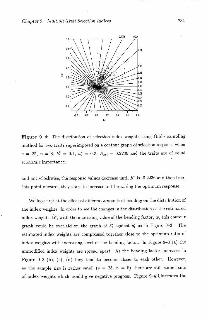
Chapter 9. Multiple-Trait Selection Indices
234
02236 0.22
0
-0.4 -0.2 0.0 0.2 0.4 0.6 0.8
bi
Figure 9-4: The distribution of selection index weights using Gibbs sampling
method for two traits superimposed on a contour graph of selection response when
= 25, ii = 8, h 2 = 0.1, h = 0.2, R0 = 0.2236 and the traits are of equal
economic importance.
and anti-clockwise, the response values decrease until if is -0.2236 and then from
this point onwards they start to increase until reaching the optimum response.
We look first at the effect of different amounts of bending on the distribution of
the index weights. In order to see the changes in the distribution of the estimated
index weights, b*, with the increasing value of the bending factor, w, this contour
graph could be overlaid on the graph of b against b as in Figure 9-3. The
estimated index weights are compressed together close to the optimum ratio of
index weights with increasing level of the bending factor. In Figure 9-3 (a) the
unmodified index weights are spread apart. As the bending factor increases in
Figure 9-3 (b), (c), (d) they tend to become closer to each other. However,
as the sample size is rather small (s = 25, it = 8) there are still some pairs
of index weights which would give negative progress. Figure 9-4 illustrates the

Chapter 9. Multiple-Trait Selection Indices 235
distribution of posterior expectations of index weights using Gibbs sampling (with
prior specification Priori) for the same design and sample size. In contrast to
Figure 9-3, posterior expectations of index weights are within the permissible
range. As a result of this one obtains more efficient selection procedures from
Bayesian decision approach.
9.6 Discussion
In this chapter, an assessment of selection procedures of half-sib families for mul-
tiple traits from estimates of parameters and from a Bayesian decision theory
approach is given and the two procedures are contrasted. A selection index com-
puted from estimates of parameters based on a finite sample size can have down-
ward bias when compared with an optimum index computed from the parameters
themselves. This is mainly because of high probability of obtaining non-positive
definite genetic matrices. If there are more traits departure from the optimum is
likely to get worse. It has been shown that rather than discarding such an index
altogether, it can be improved by bending the estimates. The bending procedure
changes the sample roots of EP
iE but the corresponding eigenvectors remain
unchanged.
However, bending the roots is not a solution to the problem, since the main
difficulty with this procedure lies in choosing the appropriate value for the bending
factor, w. Two modification procedures are used to improve selection indices:
i) the negative roots of are set to zero, and ii) the negative roots are
regressed to their mean until the most negative root becomes 0. Improved values
of selection indices are obtained from both modification methods but the second
always appears to give better selection responses than the first.
There is always appreciable prior information about the parameters and this
information may be incorporated in the construction of selection indices in a sys-

Chapter 9. Multiple-Trait Selection Indices 236
tematic way using a Bayesian approach. Two different prior specification Priori
and Prior2 are adopted (see Section 8.5.2 for these) and the values of selection
responses from these priors are compared and contrasted with unmodified and
modified results of conventional method. The use of different prior specifications
does not make significant changes in marginal posterior inferences about the se-
lection indices, except in cases where there are two traits and one has an economic
weight 0. In such cases Prior2 seems to yield better achieved responses than
Priori. It was clear that modification procedures and Bayesian methods with
different priors are rather effective with small family sizes but all methods give
similar results for larger numbers of families.
The Bayesian decision theory approach is, without doubt, preferable to the
conventional methods of computing selection indices on several grounds. Firstly,
it incorporates prior information about the population parameters into a Bayesian
selection procedure. This is impossible with the estimative procedures. The spec-
ifications of the prior information in this study do not change the marginal poste-
rior density appreciably; different prior specifications give almost identical poste-
rior expected progress. Therefore, the Bayes solution to selection appears robust
to changes in the prior assumptions. Secondly, as the Bayesian procedures give
marginal posterior expectations which are always within the parameter space one
does not have to apply some kind of modification procedure to improve the selec-
tion index.

Chapter 10
Analysis of Test Day Milk Yields of Dairy
Cows
10.1 Introduction
The genetic evaluation of dairy sires and cows for production traits in the UK
and many other countries has depended for many years on the analysis of 305-
day lactation milk production; this is commonly standardized to a period of 10
calendar months. The basis of every 305-day milk yield is a set of individual test
day yields usually taken approximately once a month over the lactation period of
305 days. An alternative approach for genetic evaluation is to analyse individual
test day records. The number of test day records may range from 2 to 12 test day
measurements. Models which directly consider records of individual test days have
become of interest and all the models incorporating records from individual test
days are referred to as test day models. This incorporation may use test day records
corrected for fixed effects such as age at calving and season of calving. These
records are then combined for evaluation purposes in a second step. Alternatively,
test day records may be considered directly in an appropriate one-step evaluation
model. Traditionally, test day lactation records have been extrapolated to a 305-
day basis following a set of well-defined rules, for example Wilmink (1987), when
predicting breeding values for sires. The number of test day records that have
been combined to provide 305-day milk yield and the procedure being employed
237

Chapter 10. Analysis of Test Day Milk Yields of Dairy Cows 238
determine the accuracy of 305-day measures. Danell (1982c) pointed out that a
disadvantage of extending test day milk yields to a 305-day basis is that the level
of production may vary over time, resulting in biased predictions of 305-day milk
yield.
One way to avoid the problem of extension of test day records into a 305-day
lactation milk production would be to use individual test day yields for genetic
evaluation of dairy sires and cows rather than estimated 305-day yields. There are
many advantages associated with the use of test day milk records of dairy heifers
in the early part of the lactation. Among these are shortening of the generation
interval and saving in expenses for housing and recording of test day milk yields
in the later part of the lactation by an early culling of bulls and cows with low
breeding values for milk production. In addition to increase in selection intensity,
the use of test day records rather than 305-day milk yields can reduce the bias due
to culling of heifers before the completion of 200 days of lactation, the minimum
length of a lactation to qualify for inclusion in sire and cow evaluation in the UK.
With regard to bias by selection, the largest potential for non-random influence in
sire evaluation is related to culling of heifers during their first lactation. Test day
records may also be used to increase the accuracy of sire selection by including
part records in addition to complete 305-day lactation records, or sires may be
selected earlier with the same accuracy. Even for completed lactation, selection
on a properly weighted index of test day records could be more accurate than
selection on predicted phenotypic records for 305-day milk yield.
In addition to the above advantages, the heritabilities of test day records have
been either the same or slightly lower than those of 305-day milk yields (Keown
and Van Vleck, 1971; Danell, 1982c; Meyer et al., 1989). Therefore, the accuracy
of a cow's genetic evaliation may be improved by using several test day yields per
cow per lactation rather than a 305-day measure. Then methods to combine test
day milk yields into a 305-day milk yield would not be necessary.

Chapter 10. Analysis of Test Day Milk Yields of Dairy Cows 239
However, the drawbacks of using test day milk records would be a large in-
crease in the number of individual test day yields to be stored on every cow (Ptak
and Schaeffer, 1993). It is also a fact that traditionally there is a strong depen-
dence on 305-day milk yield information. Therefore, this information would still
need to be provided to dairymen for management purposes. The computation of
genetic evaluations of dairy sires and cows may take a much longer time due to
the increased number of record used, and also due to the more complex statistical
models that might be needed for test day milk yields. Some additional drawbacks
are that these models contain many more parameters and need to describe the
lactation shape and include several fixed effects. Another drawback with using
individual test day records is that the conventional methods give unreasonable
estimates with increasing probability as the number of traits is increased. Hence
there is a need for a more coherent method for constructing indices. As argued in
Chapters 8 and 9, the Bayesian procedure offers such a method.
10.1.1 Literature Review
This section reviews a number of studies on the analysis of test day milk yields
in two parts: sources of variation in test day milk yields and estimates of genetic
and phenotypic parameters.
Sources of variation
Previous studies on the analysis of test day milk yields have used a wide range of
statistical models, each fitting different environmental factors. Table 10-1 gives a
summary of statistical models used by various authors. Knowledge of variation in
test day milk yields due to environmental factors used in these models is essential
for correct estimation of genetic and phenotypic parameters as well as breeding
values. As can be seen from Table 10-1, the most common ones are herd, age at
calving, month of calving, length of first period (interval between calving and first

Chapter 10. Analysis of Test Day Milk Yields of Dairy Cows 240
test), days open and calving interval. Some of the environmental factors causing
variation in test day milk yields are discussed below.
Herd effect: Auran (1973) fitted herd effects as the regression of test day milk
yields on herd average and found that herd effects accounted for approximately
25 to 40% of the total sums of squares in monthly test day yields. He reported
that the herd effect varied for various test day milk yields. The reduction in sums
of squares due to herd average was relatively less for the first and the last test
day yields than for the test day yields in the middle of lactation. He concluded
that regression on herd level would satisfactorily remove the herd effect from test •
day milk yields. However the usual way of removing the herd effect is to include
herd-year-season effects in the model. Recently Meyer et al. (1989) compared two
models, one with herd-year-season, another with herd-year-month effects. They
reported that fitting herd-year-month effects reduced residual variances consider-
ably over estimates from a model fitting herd-year-season effects, indicating the
importance of environmental effects specific to the time of test.
More recently, following a preliminary analysis to determine proper partition-
ing of the environmental variation, Pander et al. (1992) also adopted a multivariate
model with herd-year-month effects for genetic analysis. Since a subset of one of
their data sets is used in this thesis, our model will also include herd-year-month
effects.
Age effect: Age at first calving affects first lactation yield significantly (Auran,
1973; Danell, 1982a). Auran (1973) reported that the effect of age on monthly
test day milk yields decreases with advancing lactation, accounting for about 41%
of total variation at first monthly test but only about 2% for the last three test
days. This indicates that the heifers are gradually maturing towards the end of the
lactation. The effect of age at calving reported by Auran (1973) was higher than
that found by Danell (1982a). These higher results might have been caused by
the different age groupings and model used for the analysis, and the correction of
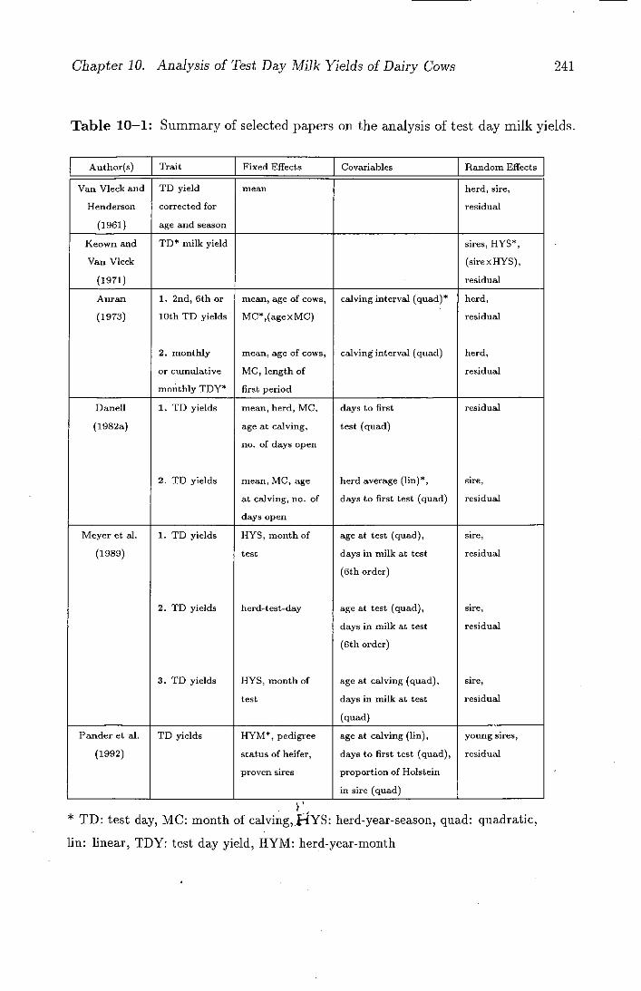
Chapter 10. Analysis of Test Day Milk Yields of Dairy Cows 241
Table 10-1: Summary of selected papers on the analysis of test day milk yields.
Author(s) Trait Fixed Effects Covariables Random Effects
Van Vieck and TD yield mean herd, sire,
Henderson corrected for residual
(1961) age and season
Keown and TD* milk yield sires, HYS*,
Van Vieck (sirexHYs),
(1971) residual
Auran 2nd, 6th or mean, age of cows, calving interval (quad) * herd,
(1973) 10th TD yields MC*,(age xMC) residual
monthly mean, age of cows, calving interval (quad) herd,
or cumulative MC, length of residual
monthly TDY* first period
Danell TD yields mean, herd, MC, days to first residual
(1982a) age at calving, test (quad)
no. of days open
TD yields mean, MC, age herd average (lin)*, sire,
at calving, no. of days to first test (quad) residual
days open
Meyer et al. TD yields HYS, month of age at test (quad), sire,
(1989) test days in milk at test residual
(6th order)
TD yields herd.-test-day age at test (quad), sire,
days in milk at test residual
(6th order)
TD yields HYS, month of age at calving (quad), sire,
test days in milk at test residual
(quad)
Pander et al. TD yields HYMt, pedigree age at calving (lin), young sires,
(1992) status of heifer, days to first test (quad), residual
proven sires proportion of Holstein
in sire (quad)
* TD: test day, MC: month of calving ,}4YS: herd-year-season, quad: quadratic,
un: linear, TDY: test day yield, 1-IYM: herd-year-month
Chapter 10. Analysis of Test Day Milk Yields of Dairy Cows 242
data for calving interval before analysis, as calving interval is negatively correlated
with age at calving.
Month/season of calving: The relationship between milk yield and season of
calving is mainly caused by seasonal variations in feeding and care, and climatic
factors. The quality and quantity of the pasture and of the supplementary feeding
are of particular importance. Auran (1973) reported that the month of calving did
not affect monthly test day milk yields appreciably, accounting for about 1.8% of
the total variation in the first test day and about 7.8% in the seventh and eighth
test days. Danell (1982a) also found that milk yield for individual test days at
the close of lactation was affected most by month of calving. He observed an
interaction between month of calving and stage of lactation. This interaction may
be viewed as differences in climatic factors and availability of the supplementary
feeding during different stages of lactation. At the early stage of the lactation,
body reserves can supply part of the energy needs, hence test day milk yields are
likely to be less influenced by month of calving.
There are other factors, such as length of the first test period, days open and
calving interval, causing variation in test day yields. These are studied by Auran
(1973) and Danell (1982a). All these studies give a clear indication that the major
environmental sources of variation in test day yields are herd-year-season and age
at calving, together accounting for more than two-thirds of the total variation.
One of the similarities among all these studies was that the effect of some of the
environmental factors was different for test day milk yields at different stages of
lactation. Herd-year-month effects explained much more variability than herd- øç the
year-season indicating the importance of timejtest.
Estimates of genetic and phenotypic parameters
Heritability: Table 10-2 summarizes the estimates of heritability of test day and
predicted 305-day milk yields obtained by different authors. The estimates of

Chapter 10. Analysis of Test Day Milk Yields of Dairy Cows 243
heritability of test day milk yields were lower than that of 305-day lactation milk
yield (Van Vleck and Henderson, 1961; Keown and Van Vleck, 1971; Auran, 1976;
Danell, 1982b; Pander et al., 1992). Estimates for test day milk yields were higher
in mid lactations. Meyer et al., (1989) also obtained similar results using restricted
maximum likelihood procedures.
These results indicate that test day yields in mid lactation have consistently
higher heritability estimates than those at the start and at the end of lactation.
Genetic and phenotypic correlations: A comprehensive review of estimates of
genetic and phenotypic correlations between predicted 305-day lactation yields
and test day milk yields is given by Pander (1992). He presented a table of pooled
estimates of genetic and phenotypic correlations from five different studies. The
general pattern in his table is that genetic and phenotypic correlations between test
day yields followed the same trend; both correlations were higher during the mid
lactation than at the beginning and the end of the lactation. However, phenotypic
correlations between test day milk yields were much lower than the corresponding
genetic correlations.
The overall conclusion about heritabilities and genetic and phenotypic correla-
tions from different studies is that test day yields in the middle of lactation have
the highest heritabilities and correlations.
10.1.2 Objectives
In dairy cattle breeding, in order to improve animals for production traits, geneti-
cally superior animals are identified on the basis of their predicted breeding values
from the phenotypic values for 305-day lactation milk yields. This is a two-step
procedure; first the phenotypic values used for genetic evaluation are predicted
from test day milk yields and then prediction of breeding values are obtained from
these predicted phenotypes. Furthermore, the predicted phenotypes for 305-day
milk yield may be slightly biased and inaccurate. Therefore there is a need to
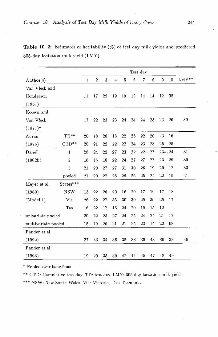
Chapter 10. Analysis of Test Day Milk Yields of Dairy Cows 244
Table 10-2: Estimates of heritability (%) of test day milk yields and predicted
305-day lactation milk yield (LMY)
Test day
Author(s) 1 2 3 4 5 6 7 8 9 10 LMY**
Van Vieck and
Henderson 11 17 22 19 19 15 14 14 12 08
(1961)
Keown and
Van Vieck 17 22 23 23 24 24 24 25 23 20 30
(1971)*
Auran TD** 20 18 20 18 22 25 22 20 23 16
(1976) CTD** 20 21 22 22 22 24 23 23 25 25
Danell 1 26 24 22 27 23 22 22-- 27 23- 24 --31
(1982b) 2 16 15 18 22 24 27 27 27 23 20 30
3 21 20 27 27 31 30 26 19 20 12 33
pooled 21 20 22 25 26 26 25 24 22 19 31
Meyer et al. States ***
(1989) NSW 13 22 26 20 16 20 17 19 17 18
(Model 1) Vic 26 22 27 35 30 30 29 30 25 17
Tas 16 22 17 16 24 20 19 15 12
univariate pooled 20 22 25 27 24 25 24 24 21 17
multivariate pooled 15 19 20 21 21 25 23 14 22 08
Pander et al.
(1992) 27 33 34 36 35 38 39 43 36 33 49
Pander et al.
(1993) 19 29 35 39 42 44 45 47 48 49
* Pooled over lactations
** CTD: Cumulative test day, TD: test day, LMY: 305-day lactation milk yield
NSW: New South Wales, Vic: Victoria, Tas: Tasmania

Chapter 10. Analysis of Test Day Milk Yields of Dairy Cows 245
find an alternative procedure based on test day milk yields to assess the animals.
REML analyses of test day milk yields have been carried out by several authors
(Meyer et al, 1989; Pander et al., 1992) but Bayesian methods have not been
applied.
So far in Chapters 4 to 9 the Bayesian analyses have been implemented to make
inferences about variance components and to evaluate selection responses using
simulated balanced univariate and multivariate one-way sire models assuming a
half-sib family structure. The main purpose of this chapter is to demonstrate
the implementation of the Gibbs Sampler with data on test day milk yields of
British Holstein-Friesian heifers. An analysis of this kind employing the Gibbs.
Sampler with a very large data set containing records on 23,873 cows and 689
sires is carried out for the first time in unbalanced univariate and multivariate half-
sib sire models. Estimates and posterior expectations of genetic and phenotypic
parameters and functions of themf are obtained from test day milk yields using
REML and Gibbs sampling methods with two different prior assumptions about
the variance matrices. REML estimates and marginal posterior expectations of
breeding values are also provided and results from the two methods are compared.
10.2 Material and Methods
10.2.1 Material
The data set studied in this chapter, which was obtained by National Milk Records
(NMR) of the Milk Marketing Board (MMB), consisted of 10 test day records
(denoted by TD1 to TD1O) of British Holstein-Friesian heifers in 7,973 herds,
which had their first test between November 1988 and October 1989. The test
day records were taken at approximately monthly intervals. Each test day milk
yield is the total of all the individual weighings taken during a 24 hour period from

Chapter 10. Analysis of Test Day Milk Yields of Dairy Cows 246
noon to noon. Milk samples were also taken for milk composition analysis at the
same time. The 305-day milk yields were predicted by linear interpolation using
the MMB's method (British Standards Institution, 1972, method 3). Lactations
shorter than 200 days were excluded from the prediction of 305-day lactation
yields. The following conditions (both lower and upper limits inclusive) were set
for a record to be included in the analysis:
age at calving was required to be in the range 20 to 40 months;
the first test had to be between day 4 and 45 of lactation;
the interval between consecutive tests was between 20 and 50 days.
Table 10-3 displays the structure of the data set. On average, 29% of herd
year-month categories had only one record; these were discarded from the full data
set . The resulting data set is described in column 2 of the table, and henceforth
referred to as the reduced data set. The reduced data set consisted of records from
23,873 daughters of 40 proven and 649 unproven sires. The number of daughters
per proven sire varied between 187 and 1,371 while the corresponding figures for
unproven sires were between 1 and 31 in the reduced data set. About one-fifth
of cows in the reduced data set were offspring of the young sires. In the reduced
data, the average number of records per herd-year-month was 3 with a maximum
number of records of 25. All of the individual test day milk yields were expressed
in kg per test day (kg milk day').
10.2.2 Statistical Methods
The following univariate and multivariate analyses were carried out on the reduced
data set assuming multivariate normality and a half-sib sire model.
i) Individual test day milk yields analysed assuming fixed herd-year-month
effects;
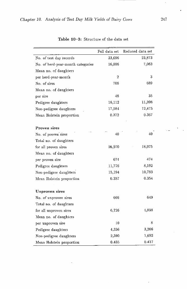
Chapter 10. Analysis of Test Day Milk Yields of Dairy Cows
Table 10-3: Structure of the data set
Full data set Reduced data set
No. of test day records 33,696 23,873
No. of herd-year-month categories 16,886 7,063
Mean no. of daughters
per herd-year-month 2 3
No. of sires 706 689
Mean no. of daughters
per sire 48 35
Pedigree daughters 16,112 11,398
Non-pedigree daughters 17,584 12,475
Mean Holstein proportion 0.372 0.367
Proven sires
No. of proven sires - - 40 40
Total no. of daughters
for all proven sires 26,970 18,975
Mean no. of daughters
per proven sire 674 474
Pedigree daughters 11,776 8,192
Non-pedigree daughters 15,194 10,783
Mean Holstein proportion 0.357 0.354
Unproven sires
No. of unproven sires 666 649
Total no. of daughters
for all unproven sires 6,726 4,898
Mean no. of daughters
per unproven sire 10 8
Pedigree daughters 4,336 3,206
Non-pedigree daughters 2,390 1,692
Mean Holstein proportion 0.435 - 0.417
247
Chapter 10. Analysis of Test Day Milk Yields of Dairy Cows 248
Individual test day milk yields analysed assuming random herd-year-month
effects;
All ten test day milk yields analysed simultaneously assuming fixed herd-
year-month effects.
The second type of analysis is open to the objection that if herd-year-month ef-
fects are treated as random then the model should include a variance component
for herds. It was not possible to apply such a model because the herds themselves
are not identifiable in the data. The analysis is included, however, because it
demonstrates how Gibbs Sampler can be applied to a more complex model than
the first. For the estimation of genetic and phenotypic parameters, univariate and
multivariate restricted maximum likelihood (REML) analyses for i) and iii) were
carried out using REML programs. Then the posterior expectations of parame-
ters of interest were obtained using the Gibbs sampling procedure. Finally, the
results from REML and Gibbs sampling were compared. Relationship among sires
through paternal grandsires were not included in the analysis.
For the analysis of the above models i), H) and Hi), sires were assumed to
be be unrelated. In order to minimize any bias from selection of sires for dairy
production, effects for proven sires were considered as fixed so that their daughters'
records contributed to the estimation of the variance within but not between sires.
This implied the assumption that residual variances were homogeneous for
daughters of both types of sires, proven and unproven ones.

Chapter 10. Analysis of Test Day Milk Yields of Dairy Cows 249
10.3 Univariate Analyses of Test Day Milk Yields
10.3.1 Treating herd-year-month effects as fixed
Model
Suppose that there are s,, proven sires and S q unproven sires (new or young sires),
and that there are observations on N daughters of proven sires and on Nq daugh-
ters of unproven ones. Let Yji denote the milk yield for a particular test day
measured on the jth daughter of sire i and let cj, h(ij) denote the vector of c
covariates and the herd-year-month group for this daughter. The covariates in-
cluded in the analyses were pedigree status of the heifer (0 = pedigree or grade
(registered), 1 = non-pedigree (non-registered), age at calving, day of lactation.
for first test and proportion of Holstein in sire) and the herd-year-month group
for this daughter.
If we take sire effects to be fixed for proven sires and random for unproven
ones then we might assume the following half-sib sire model
= 1,. . s, proven sires
Yji = h(ij) + - e) + s + ejj i = Sp + 1,. . . , Sp + 5q, unproven sires
j=l,...,n (10.1)
Here the a's represent herd-year-month effects, /3 the vector of regression coeffi-
cients for the covariates and the s i the sire effects for proven and unproven sires.
The ej are assumed to be N(O, or ) and independently distributed given a, /3, s
and o,, . In matrix terms, this may be written as
y=Ha+C/3+Ds+e (10.2)
where H defines the herd/year/month membership of each daughter, C contains
the centred values of the covariables and D specifies the sire fathering each daugh-

Chapter 10. Analysis of Test Day Milk Yields of Dairy Cows 250
ter. Since all test day records are complete, all vectors y and e have length
N = N + N, the number of records. The vector of fixed effects, a, has length g,
the number of herd-year-month groups. The vector of regression coefficients, 0,
has length c, and s has length s = Sp + 5q, the number of proven and unproven
sires. Correspondingly, the matrices H, C and D have dimensions N x g, N x c
and N x s, respectively. The design matrix D and sire vector s can be partitioned
as follows
ID o 1 1s1 D= L 0 D s=
q j [sq j
where s, and S q are the vectors of effects of proven and unproven sires and D and
D q are matrices associating these effects with records. As explained in Section
10.2.2, the sire effects are taken to be fixed and random for proven and unproven
sires respectively. - - - - -
The following assumptions are made
E(ya, j3,s,o,o)=Ha+C/3+Ds, E(s)=O, E(e)=O,
Var(s q ) = Var(e) = INC, Cov(s q , e) = 0,
2 2 2 Var(y a, $,s,a3 ,c6 )
' Ne
If N denotes the total number of daughters observed then the likelihood func-
tion is, apart from a constant factor
2 f(y a,t3,s,o)
oc (aY4Nexp{_ {(y— Ha - C - Ds)'(y —Ha - C - Ds)]}. 2 0,2
(10.4)

Chapter 10. Analysis of Test Day Milk Yields of Dairy Cows 251
Prior distributions
For the prior distribution, we might take a, 3, s, to be independently uniformly
distributed,
f(a, 0, si,) cx constant, (10.5)
the elements of 5q to be independent,
N sq (O 1sq0), (10.6)
a to be inverse-x 2 with probability density function given by
2 2 / 2 —4(u+2) exp / v5s\
f(c3 "s, s) cx (as) c\20-S-)
a ? 0, (10.7)
(denoted by Y 2 (v8, s)) and 0-2 to be inverse-x 2 with parameters 1'e s and prob-
ability density function independently of c
Jae I e , 84 ()_4(u2) exp / rI 21 2
>0. (10.8) 2a2 6
Posterior density function
The posterior probability density function for a, 0, s, a, a is given by
f(a ) /3,s,a,o y)
k2)- 1 lcx (N+Ve +2)( 2)_4(Sq+L/s+2) exp (s q s q + vs s)]U2
{ 1 x exp _[(y_Ha_c/3_Ds)'(y_Ha_C$_Ds)+ves]}.
2a (10.9)
Full conditional posterior densities
The full conditional posterior distributions of a, /3, 5p, S q , a 2 and a are obtained
from the joint posterior probability density function in (10.9).

Chapter 10. Analysis of Test Day Milk Yields of Dairy Cows 252
To obtain the full conditional distributions of a, 13, s, and 5q, note that if a
vector 0 has a probability density function proportional to
exp [- (O'Ao - 26'a)]
with A positive definite then its distribution is N(Aa, A -1 ):
Conditional posterior distribution of a. The posterior probability density func-
tion of a is proportional to
1 exP{__[aHHa_2a
/H(Y
I_Cs_ Ds) ]}
so the conditional distribution of a is
[a 10, s,a,o,y} = N9 (G_1H'(y CO - Ds), cG') , (10.10)
where G denotes H'H, the diagonal matrix giving the frequencies of the g herd
year month groups.
Conditional posterior distribution of 0. The posterior probability density func-
tion of 3 is proportional to
exP 1
{_CCs_2sC(Y_Ha_Ds)]}
so the conditional distribution of 0 is
[/3 a, s, c, a, yJ = N, ((C'CYlC'(y - Ha - Ds), c (C'C) 1 ) , ( 10.11)
where (C'C)l is the matrix of corrected sums of squares and products of the
covariables.
Conditional posterior distribution of s. The posterior probability density func-
tion of s, is proportional to
exp - 1
[ p sFD
FDs - 2s2D(y - Ha - C25)] },
{
20 .2
so the conditional distribution of s, is
2 2 Is a,$,sq ,a3 ,a,y] = (ç1 D(y - Ha - C/3), aF), (10.12)
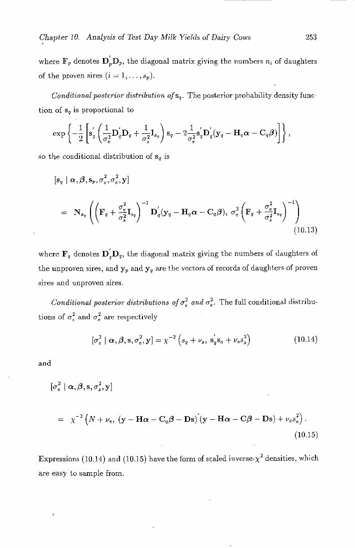
Chapter 10. Analysis of Test Day Milk Yields of Dairy Cows 253
where F denotes D,DP, the diagonal matrix giving the numbers n i of daughters
of the proven sires (i = 1,. . . ,
Conditional posterior distribution of S q . The posterior probability density func-
tion of S q is proportional to
( 11, ( /i exp j-
D q Dq + - 2 sD(yq - Hq a -
so the conditional distribution of 5q is
[sq I QB,Sp,Us 2, 2Oe,Y]
2 -1 2-1
= N sq ((F + 4I sq ) D(yq - Hq a - Cq $), a (F + Isq)
) as
(10.13)
where F q denotes DD q , the diagonal matrix giving the numbers of daughters of
the unproven sires, and y, and Y q are the vectors of records of daughters of proven
sires and unproven sires.
Conditional posterior distributions of c 2 and a. The full conditional distribu-
tions of a and a are respectively
[a2 /3sa2y] -2 3 a, = x (s q + 5q5q + ( 10.14)
and
[
2 cre a,$,s,o,y]
= X 2 (N+Ve, (y—Ha—C q $—Ds)'(y—Ha—C)3— Ds) +ves).
(10.15)
Expressions (10.14) and (10.15) have the form of scaled inverse-x 2 densities, which
are easy to sample from.

Chapter 10. Analysis of Test Day Milk Yields of Dairy Cows 254
10.3.2 Treating herd-year-month effects as random
Model
The model (10.2) is slightly modified to include random herd-year-month effects
with expectation zero and a mean herd effect p. The model is then given by
Liii + Ha + C3 + Ds + e
(10.16)
where a represents a vector of random rather than fixed herd-year-month effects
in (10.2), 1 is a vector of N l's and H, C, $, s and e are the same as before. The
following assumptions are made about this model
E(y I ,Lh, CC, fl,ah ,cS ,CC ) = Phi + CO + Ds, E(a) = 0, E(s q ) = 0, E(e) = 0,
Var(a) = I9 cr, Var(s q ) = Isq cr, Var(e) =
Cov(s q , e) = 0, Cov(a, sq ) = 0, Cov(a, e) = 0,
Var(y rih,a,$,c,c,a) = V = IN U2.
The likelihood function is the same as (10.4).
Prior distributions
For the prior distribution, we might take Ph, 3, s, to be independently uniform,
cc constant, (10.17)
a to satisfy
a I Ch - N9 (ph19 , Isqo) (10.18)
and the prior distributions of s 9 , a 2 and a are the same as (10.6), (10.7) and
(10.8), respectively. The prior distribution of a 2 is taken to be inverse-x 2 with
parameters h, s and probability density function
2 2 2 -i(uh-j-2) ( VJ5\ 2 Vh,Sh) cx (oh)
-
--
-
-- )
Cj ~ 0 . (10.19) 2a 2

Chapter 10. Analysis of Test Day Milk Yields of Dairy Cows 255
Posterior density function
The joint posterior probability density function for p, a, 0, s, o, o, c is given
by
f(ph,a,/3,s,c,c,a y)
2 )_4(N+Ve+2)(2)_(S+Vs+2)( 52)_(9+Vh+2) cx (0-'
[1 [ + v5s) ] exp I( 1
a ]x exp _(sq s q
[ }
x exp{_[(Y_Ha_c/3_Ds)'(Y_Ha_cs_Ds)+vs]}.
(10.20)
Full conditional posterior densities
Conditional posterior distribution of ph. The posterior probability density function
Of Ph is proportional to
[
--L exp (pii9 - 2Pha ' la )] 2 h
so the conditional distribution of ph is
(E
2 2 2 ah [ph a,/3,s,a,c 3 ,a,y] =
N9 I - 9/, (10.21)
Conditional posterior distribution of a. The posterior probability density func-
tion of a is proportional to
I 1 2 2exp -, [a'(aI9 + aH'H)a - 2a (cphi g + aH'(y - - Ds))] }, 2co

Chapter 10. Analysis of Test Day Milk Yields of Dairy Cows 256
so the conditional distribution of a is
2 2 2 [a I Ph, 13 ,s,ah, Ors) ore, y]
= N9 ((oI9 + oHH) 1 [4/2h1 9 + cH(y - CO - Ds)]
C 2 hCe
2(O e
2I9
+ 0_ 2H'H)' (10.22)
Conditional posterior distributions of 0, s, and 5q The conditional densities of
13, s, and 5q are similar to those given in (10.11), (10.12) and (10.13), respectively
and are as follows
[13 1 Ph, a, s, a, o, c, = N ((c'cylc'(y - Ha - Ds), a(CCY'),
(10.23)
[s Ph, a, /3, 5q, a, a, y] = N3 (F;'D(y - Ha C$), aF'),
(10.24)
and
22 2 [Sq
2-1
= N sq ((F + D 9 (yq - H qa - C qØ), Or (Fq + Is
(10.25)
Conditional posterior distribution of o- , a and a. The full conditional dis-
tributions of c, a and cr are respectively
2 2 -2
[h ph,a,P,s,c3,a,y] = (g + vh, (a - phi g ) (a - Ph + vhs2h)
(10.26)

Chapter 10. Analysis of Test Day Milk Yields of Dairy Cows 257
2, [a ,1h,a,13 ,S,ah,a,y] = x2 (s q + us , S ' q S q + uss) (10.27)
and
2 2 [a ith,Q,$,S, 5h,s,YI
= _2(N+p,(y_ Hoe _Cq_Ds)'(y_Ha_C$_Ds)+ues).
(10.28)
10.4 Multivariate Analysis of Test Day Milk Yields
10.4.1 Model
If the design matrices H and D and the matrix for covariables C are the same
for all test days (or more generally for any t traits), then the multiple-trait model
can be written as a direct extension of (10.2). Then y, a, $, s and e are replaced
by matrices Y, A, B, S and E, which are respectively N x t, g x t, c x t, s x I
and N x I, with each column corresponding to a different trait. The matrix S can
be partitioned as ['j where S, and 5q are the matrices of effects of proven and
unproven sires. The model for the multiple-trait analysis becomes
Y = HA + GB + DS + E.
When deriving the likelihood and the posterior density functions if is convenient
to write Y, A, B, S and E in vector form using the vec operator, for example
yi
Y2 Yv = vecY =
Yt

Chapter 10. Analysis of Test Day Milk Yields of Dairy Cows
258
If also a, /3, s, and e denote vecA, vecB, vecS and vecE respectively and 0
denotes the direct or Kronecker product then the model may be expressed as
Yv = ( It 0 H)a + (It 0 C)/3 + (It 0 D)s + e 0 , ( 10.29)
where Yv is constructed to form a single vector by stacking the columns of the
matrix Y one under another (Henderson and Searle, 1979). The operation has
been referred to as the column string or stack of Y and the pack of Y, with vecY
(for "vec of columns of Y") being the notation currently in use. However, for
the sake of simplicity Yv will be employed throughout this chapter. The following
assumptions are made,
E(s qv) = 0, E(e) = 0,
Var(s qv ) = Es 0 ]Isq Var(e) = E e 0 'N, Cov(s qv , e) = 0.
Then, given civ , 13 ,,, s,,, E 5 and E e
Yv - NNt ((Ii 0 H)a,, + (It 0 c)t3 + (It 0 D)s,,, E e 0 IN).
The likelihood function is, apart from a constant factor
f(y ,, )3 , s, E)
cc E,e -4N exp {- [(Yv - (L 0 H)a,, - (I 0 C)13 - (I 0
X (E e 0 IN) — ' (yv - (L 0 H)a,, - (It 0 C)$,, - (L 0 D)sv)] } (10.30)
10.4.2 Prior distributions
Prior distributions for the univariate analysis of test day milk yields treating herd-
year-month effects as fixed can conveniently be generalized to multivariate analy-
ses. These distributions for the model parameters are as follows.
f (a,,, )3, si,,,) cc constant, (10.31)
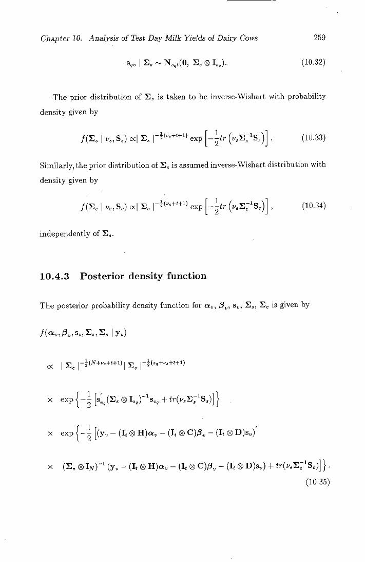
Chapter 10. Analysis of Test Day Milk Yields of Dairy Cows 259
5 qv I E3 r-j N sqt(O J s 0 Is q ). (10.32)
The prior distribution of E 3 is taken to be inverse-Wishart with probability
density given by
(us+t+1) 1-2
1
v3 , S 3 ) E3 L exp tr ( ,/, E, )1 (10.33) Similarly, the prior distribution of Ee is assumed inverse-Wishart distribution with
density given by
f(Ee 'e s 6 ) E e exp [_tr (ve E 1 S e)], (10.34)
independently of Y2.
10.4.3 Posterior density function
The posterior probability density function for a,, 13, s, E 3 , E, is given by
f(Qv,I3 v ,Sv,Es,e 1 Yv)
Ee 4(N+ve +t+1) —(5q+vs+t+1) OC
x exp H I 0 Isq )'svq + tr(vJi1Ss)] }
x exp {- [(yv - ( I 0 H)a —('20 C)p - (I 0 D)s)
x (E0 0 TN) (Yv - ( I 0 H)a - (I 0 C)/3 0 - ( I (D D)s) + tr(veE1Se)] }.
(10.35)

Chapter 10. Analysis of Test Day Milk Yields of Dairy Cows 260
10.4.4 Full conditional posterior densities
Conditional posterior distribution of ct. The posterior probability density func-
tion of a is proportional to
exp {- [a(It ® H) ' (E e 0 IN ) — '(It 0 H)a
so the conditional distribution of a,, is
[a
= N9 ((Ii 0 H'H)_l(It (3 H)'(y - (I t 0 C)$ - (It 0 D)s), E ® (H'H)').
(10.36)
Conditional posterior distribution of i• The posterior probability density
function of 13,, is proportional to
exp [)3 ' (I 0 C)'(e 0 IN )- '(It0 C)13,,
- 20(I 0 C)'(Je 0 IN 1 (yn - (I 0 H), - (I ® D)s)] }
so the conditional distribution of 3, is
[P
= N0 ((Ii (D C'C)_l(It 0 C)'(y, - (It ® H)a,, - (It 0 D)s,,), Z, 0 (c'c) -'). (10.37)
Conditional posterior distribution of sr,. The posterior probability density
function of s i,,, is proportional to
h exp [si
(I 0 D)'( 6 0 IN)- ' (It 0 D)s,,
- 2sj1j 0 Dp ) ' 1 ( (Ee 0 'NYS'pv - (I 0 H )a - (I 0
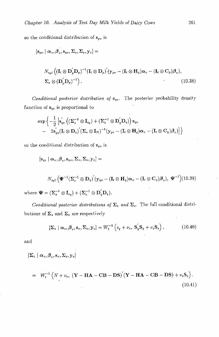
Chapter 10. Analysis of Test Day Milk Yields of Dairy Cows 261
so the conditional distribution of sP V is
a v ,$,sqv , Is, le, yv] =
N5 ((Ii 0 DD)-1(I (3 D)'(y - (I t 0 H)a - (It 0 C2)i3 ),
E 6 ® ( D' D,) (10.38)
Conditional posterior distribution of Sqv. The posterior probability density
function of Sqv is proportional to
1 1 ' exp c— [sqv ((1
0 Is,) + (1 ® D q Dq )) 5 qv
- 2s q v(L 0 D,) (M e o IN) (Yqv - (I t 0 Hq)av - (It 0 Cq)/3v)] }
so the conditional distribution of 5qv is
[sqv I 0v ,$,S pv , I s , E e ,Y v J
N8 q t (w -1 (E -1 0 D q ) (yqv - (I t 0 Hq)ctv - (I t ® Cq)$), t_1)(10.39)
where IF = ( Is ' 0 Tsq ) + (Ee 0 DDq ).
Conditional posterior distributions of E 3 and E e . The full conditional distri-
butions of E 5 and E are respectively
a, Iv' Sv, Ee, y] = W[1 (sq + Vs, S q S q + v8 s 8 ) ( 10.40)
and
a, $,, Sv, E3 , Yv]
= WI'(N+v, (Y_HA_CB_DS)(YHA_CB_ DS) +VeSe).
(10.41)
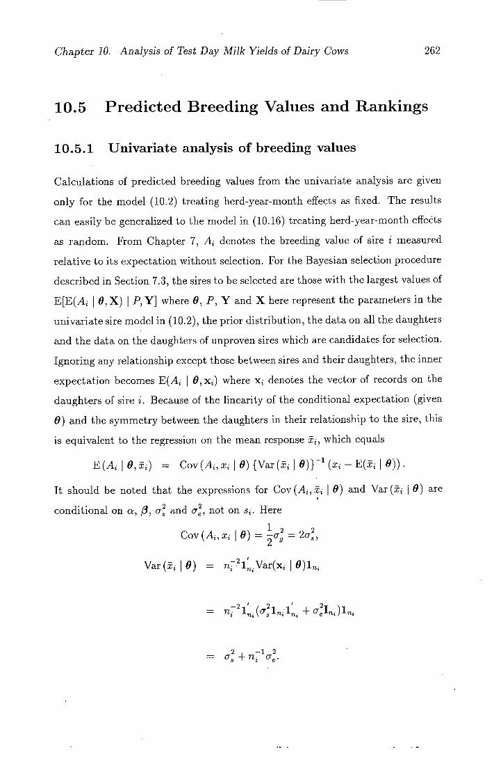
Chapter 10. Analysis of Test Day Milk Yields of Dairy Cows 262
10.5 Predicted Breeding Values and Rankings
10.5.1 Univariate analysis of breeding values
Calculations of predicted breeding values from the univariate analysis are given
only for the model (10.2) treating herd-year-month effects as fixed. The results
can easily be generalized to the model in (10.16) treating herd-year-month effets
as random. From Chapter 7, A i denotes the breeding value of sire i measured
relative to its expectation without selection. For the Bayesian selection procedure
described in Section 7.3, the sires to be selected are those with the largest values of
E[E(A 9,X) I P, Y] where 9, F, V and X here represent the parameters in the
univariate sire model in (10.2), the prior distribution, the data on all the daughters
and the data on the daughters of unproven sires which are candidates for selection.
Ignoring any relationship except those between sires and their daughters, the inner
expectation becomes E(A j 1 0, x1 ) where x1 denotes the vector of records on the
daughters of sire i. Because of the linearity of the conditional expectation (given
9) and the symmetry between the daughters in their relationship to the sire, this
is equivalent to the regression on the mean response xi, which equals
E (A i 1 0, ±) = Cov(A, xj 10) {Var (xi 9) }1 ( - E( 9)).
It should be noted that the expressions for Coy (A i , xi 9) and Var (± 9) are
conditional on a, $, a 2 and o, not on s. Here
Cov(A,± 12
6) = = 2
Var(± ) = nT?1.Var(xi I 9)1.
—2
= n +
2 —1 2 = °e

Chapter 10. Analysis of Test Day Milk Yields of Dairy Cows 263
Hence
Thi
2 2 2-1
E(A 6,x) = za 8 (na3 + E(x - - j3 (c - c)) j=1
2h2
= 4 + (n - 1)h2 - ah(j) - P (Cij
(10.42)
10.5.2 Multivariate analysis of breeding values
Suppose that the economic value of the animal depends linearly on I traits, so that
a I-vector a of economic values may be specified. Then the aggregate breeding
value of candidate i, as given in Chapter 9, is Hi = a'gj where gi is a vector of
genetic values corresponding to the observed traits. We seek to select animals for
which this breeding value is large. Hence we consider its conditional expectation
given the measurements x i for each candidate.
For the multivariate half-sib family structure in model (10.29) the expectation
becomes E(a'g j 10, x 2 , . . . , x 1 ) = E(a'gi 10, xi) by the same argument as in
Section 10.5.1. Then
Cov(g, 9) = 2J 3
Var(* = 1
9) [n( 5 + E) + n(n - i)E 5 ]
= ni
= s +flj 'E e .
Hence
E(a'g j 10, .j) = 2a'E8 n(n 3 + E 6)i(k - E(k 1 9))

Chapter 10. Analysis of Test Day Milk Yields of Dairy Cows 264
Ui
= 2aE(n€E3 + E {xjj - 0h(ij) - B(c1 - j=1
(10.43)
where a is taken to be 110 for test day milk yields throughout this chapter. The
vector of index weights is therefore the posterior expectation of 2(n 3 +E e ) 1 5a.
10.5.3 Comparing rankings of unproven sires
Given a set of candidates, any selection procedure provides a ranking of the can-
didates which may be based on an assessment of their breeding values, either es-
timates or posterior expectations. We treat the unproven sires as candidates here
in order to illustrate methods of comparing selection procedures. Comparisons
of interest then include those between Bayesian and REML procedures, between
Bayesian procedures based on different prior distributions, and between proce-
dures using all 10 test day records or the first few, or a summary such as 305-day
lactation milk yield. Possible methods of comparison include plotting the ex-
pected or estimated breeding values against each other, and examination of ranks
assigned by different methods, especially for the best candidates according to each
procedure.
A further method treats one selection procedure as a standard, and attempts
to measure the potential loss in expected progress from selection if one or more
other procedures were used instead. When the effect of omitting some traits is
being considered, the standard procedure would be one based on all the available
traits. Let e 1 , e 2 and so on denote the posterior expected (or estimated) breeding
values according to the standard procedure arranged in descending order. If n
candidates are to be selected, then the average posterior expected breeding value
of the selected has a maximum of (el + e 2 + . .. + e)/n. A plot of this average
against n 0 might be useful when deciding how many to select.

Chapter 10. Analysis of Test Day Milk Yields of Dairy Cows 265
Given n, any other selection procedure may lead to a different set of n0 can-
didates, and this will give a lower average posterior expected breeding value. A
plot showing these averages for different selection procedures is necessarily biased
in favour of the standard procedure, but it gives an indication of whether there
are substantial differences between them.
10.6 Gibbs Sampling
The implementation of the Gibbs Sampler is carried out for univariate and multi-
variate analyses in the way described in Chapters 4 and 8. Random samples are
generated from the joint posterior distribution through successively drawing sam-
ples from the full conditional posterior densities of appropriate sets of parameters
and updating the Gibbs Sampler. Based on theoretical arguments (Raftery and
Lewis, 1992) and on our experience with simulated data, we used the single long
chain method without discarding the so-called warm-up iterations for the final
sample.
Univariate Gibbs sampler procedures for models (10.2) and (10.16) are run
twice. In the first run, some arbitrary starting values are assigned to the parame-
ters of interest and the results of 1,200 iterations are stored. After examining the
samples for convergence, the first 200 iterations are discarded and averages based
on the last 1,000 iterations are obtained. In the second run, these averages are
used as starting values and 1,000 iterations are stored as samples on grounds that
the chain may have reached the equilibrium distribution. Therefore the marginal
posterior inferences about the parameters in models (10.2) and (10.16) are based
on 1,000 iterations of the Gibbs Sampler. Convergence in the final samples is
reached within a few iterations. The prior degrees of freedom v 3 , v and Ph are
chosen to be unity.

Chapter 10. Analysis of Test Day Milk Yields of Dairy Cows 266
In the multivariate Gibbs Sampler procedure, two separate sets of iterations
are run with different values for the matrices S, and S of hyperparameters with
degrees of freedom v, = V6 = 10. These are as follows:
Prior information based on the results of early studies. A common first order
autoregression structure is assumed for 5, and S of the form
1 5 . .. b9 1 5 . . .69
5 1 b . . . b b 1 5 . . . 58 S, = a, , =
b9 b8 7 1 69 8 b7 ... 1
where a, and a 6 are the prior hyperparameters for sire and residual vari-
ances and JbI < 1 is the autocorrelation coefficient. All three parameters a,,
b and a 8 are obtained from Pander's thesis (1992) as 0.734, 0.95 and 7.865,
respectively. This prior information is referred to as PRIORI. The follow-
ing comments can be made in relation to PRIORI: a) prior variances are
assumed equal over test days; b) 5, and 5, are proportional, so that a priori
one would use the base index; c) the correlations between test day records
which are far apart in time appear too low; d) no structure is assumed for
1, and E,; e) using an unrealistic form for S. and S, provides an assessment
of the robustness of the Bayesian procedure.
Prior information based on the results of REML estimates. REML estimates
of sire and residual variance matrices for the same data are used as starting
values for the hyperparameters 5, and 5, and the resulting prior informa-
tion is denoted by PRIOR2. This method is open to the objection that it
uses the same data twice and hence provides an over-optimistic assessment
of precision about the posterior distribution. On the other hand, only 10
degrees of freedom are associated with 5, and S,
Prior information for the remaining parameters, i.e., covariates, and fixed ef
fects is chosen arbitrarily to be uniform, as none of the published works gave

Chapter 10. Analysis of Test Day Milk Yields of Dairy Cows 267
estimates of these parameters. The total number of samples saved for each un-
known parameter in univariate and multivariate analyses are 1,000 and inferences
about these parameters are made by computing directly summary statistics from
1,000 samples. Due to computer storage limitation, not all Gibbs samples and
conditional means and standard deviations could be saved for all parameters.
10.7 Results
Raw phenotypic means and standard deviations for individual test days and 305-
day lactation milk yield in the full and reduced data sets are given in Table 10-4.
Average milk yields per test day exhibit the typical form of a dairy cattle lactation
curve with a peak around day 40 corresponding to test day 2. Milk yield then
declines to about 60% of peak yield in month 10. The variation in test day milk
yield declines gradually from TD1 to TD7.
10.7.1 Univariate analyses
Results from the model treating herd-year-month effects as fixed
Univariate REML estimates of parameters: REML estimates of the variance com-
ponents, a, a and and heritability h2 , together with their standard deviations,
for individual test days and 305-day lactation milk yield are shown in Table 10-5.
The estimates of residual variances are most variable early and late in lactation.
These estimates decrease from TD1 to TD8 and increase toward the end of lacta-
tion. The estimate of sire variance for individual test day milk yields tends to be
higher later in the lactation.
The heritability estimate for 305-day lactation milk yield (LMY) is 0.49. The
estimate is rather lower for the first three test days than others. This finding

Chapter 10. Analysis of Test Day Milk Yields of Dairy Cows 268
Table 10-4: Raw phenotypic means and standard deviations (SD) at individual
test days and 305-day lactation milk yield (LMY) for full and reduced data sets.
Trait Full data
mean SD
Reduced data mean SD
Reduced data set Proven sires Young sires mean SD mean SD
TD1 19.45 4.05 19.45 4.02 19.43 4.06 19.51 3.88
TD2 20.63 3.95 20.66 3.90 20.68 3.92 20.58 3.80
TD3 19.66 3.95 19.70 3.91 19.71 3.94 19.65 3.82
TD4 18.56 3.87 18.58 3.82 18.61 3.83 18.48 3.78
TD5 17.57 3.79 17.58 3.75 17.61 3.77 17.48 3.69
TD6 16.74 3.74 16.75 3.71 16.78 3.72 16.65 3.66
TD7 16.16 3.76 16.16 3.73 16.19 3.76 16.13 3.63
TD8 15.51 3.75 15.59 3.74 15.60 3.75 15.52 3.70
TD9 14.55 3.75 14.69 3.75 14.70 3.76 14.65 3.70
TD10 12.89 3.86 12.99 3.88 12.94 3.89 13.17 3.85
LMYt 52.55 9.35 52.66 9.28 52.68 9.31 52.58 9.15
* Means and standard deviations for LMY are divided by 102
is not only attributable to high residual components, but also to a rather small
component of the sire variance and the low estimates indicate that the first part
of the lactation is least heritable. The general pattern of heritability estimates for
test day milk yields, as observed by Pander et al. (1993), is an increase from TD1
to TD8 followed by a decrease. The increase in heritabilities is more a function of
increasing sire variances than of decreasing residual variance components. Other
studies with an exception of Pander et al. (1992 and 1993), found heritabilities
for test day milk yields to be lower than the estimates obtained in this study (see
Table 10-2).
Univariate REML estimates of regression coefficients for covariates are pre-
sented in Table 10-6. In general, the coefficients for age at calving and days of
lactation for first test are highest early in lactation. The effect of age at calving
is the largest on the first test day milk yield and then reduces gradually with

Chapter 10. Analysis of Test Day Milk Yields of Dairy Cows 269
advancing lactation. Days of lactation for first test (interval between calving and
first test) has the highest effect on TD1. The most variable coefficient is that for
pedigree status.
Univariate Gibbs sampling results: Posterior expectations and standard devi-
ations of variance components and heritability from univariate Gibbs sampling
analyses based on 1,000 iterations are presented in Table 10-7. When compared
with the REML estimates, posterior expectations are slightly higher but the stan-
dard deviations are lower than those of REML results. Similar conclusion can
therefore be drawn here. Table 10-8 gives posterior expectations of regression
coefficients for covariates. It is striking to observe that these are almost the same
as the corresponding REML estimates except for pedigree status.
Results from the model treating herd-year-month effects as random
The purpose of treating herd-year-month effects as random was to demonstrate
how the Gibbs sampling procedure handles a model which includes herd effects
and more than two variance components. In this section, only the posterior expec-
tations of variance components, heritability and covariates from Gibbs sampling
analysis will be presented and the results will be compared with those given in Ta-
bles 10-7 and 10-8. Two separate heritabilities are calculated; first one is obtained
in the usual way, = 4o/(c+o) and the second one is h = 4a/(a+u+c).
Posterior expectations and standard deviations of variance components, o, a and
and heritabilities h, h, are given in Table 10-9. As compared with the results
of Table 10-7, posterior expectations of a 2 S
are higher in Table 10-9 and those of
ae are similar. The first heritability h is much higher than the second one h.
Posterior expectations of h 2 under the model (10.16) (see Table 10-9) are substan-
tially higher than those found for the model (10.2) (Table 10-7). This is largely
due to an increase in the sire variance component.

Chapter 10. Analysis of Test Day Milk Yields of Dairy Cows 270
Table 10-10 presents the marginal posterior expectations of regression coeffi-
cients for covariates. The expectations in this table for days of lactations for first
test (DL) seem to agree with those in Table 10-8. However the values for PS, AC
and HP are slightly different across test day milk yields.
10.7.2 Multivariate analysis
Multivariate REML estimates of parameters: Multivariate REML estimates of
sire and residual variance matrices for test day milk yields are given in Table 10-
11. Estimates of residual variance are highest for TD1 and decreasing thereafter
during the first eight months of lactation. As in the univariate analysis, sire
variance estimates for test day milk yields show an irregular pattern, possibly due
to monthly effects within herd-year-month. However these estimates seem to vary
less over test days than those of residual variances. Sire variance component is
the highest at TD8. The lowest one is observed in the first month of lactation.
Residual covariances are highest at the beginning of lactation and decrease as
lactation progress. However sire covariances increase steadily from first to seventh
lactation, giving the highest in covariances after mid lactation.
Table 10-12 presents multivariate estimates of heritability and genetic and
phenotypic correlations for test day milk yields. The estimate of heritability is
lower (0.28) for TD1 than for the others. Heritability estimates are generally
higher during the second half of the lactation than the first half. Estimates for
TD5 - TD7 are similar (0.39). The highest estimate of heritability of all the test
days is obtained for TD8 (0.42). In general, genetic correlations among test day
milk yields are high (0.62 to 0.99). The highest genetic correlations are obtained
between TD4 and TD7, and the correlations decrease as intervals between test
increase. It can be seen from Table 10-12 that the phenotypic correlations follow
similar pattern but are lower than the genetic correlations, ranging from 0.30 to
0.76.

Chapter 10. Analysis of Test Day Milk Yields of Dairy Cows 271
Table 10-5: Univariate REML estimates and standard deviations (SD) of vari-
ance components and heritability for individual test day records and 305-day lac-
tation milk yields.
SD SD a, SD SD
TD1 0.6852 0.2055 9.4546 0.1045 10.1398 0.2191 0.2703 0.0759
TD2 0.6646 0.1838 8.6609 0.0957 9.3255 0.1976 0.2851 0.0736
TD3 0.6175 0.1796 8.5952 0.0949 9.2127 0.1934 0.2681 0.0731
TD4 0.7000 0.1898 7.9816 0.0883 8.6816 0.1993 0.3225 0.0809
TD5 0.7448 0.1798 7.4571 0.0825 8.2019 0.1891 0.3632 0.0802
TD6 0.7229 0.1842 7.1871 0.0796 7.9100 0.1913 0.3656 0.0852
TD7 0.7001 0.1736 7.0552 0.0781 7.7553 0.1817 0.3611 0.0819
TD8 0.7798 0.1733 7.0218 0.0776 7.8016 .0.1821 0.3998 0.0805
TD9 0.7611 0.1792 7.1057 0.0786 7.8668 0.1872 0.3869 0.0828
TD10 0.6953 0.1840 8.1875 0.0905 8.8828 0.1956 0.3131 0.0768 LMY* 6.2225 1.2434 44.8195 0.4961 51.0421 1.2879 0.4876 0.0862
* Estimates of a, a and a and their standard deviations for LMY are divided by 10.
Table 10-6: Univariate REML estimates of regression coefficients for covariates,
pedigree status (PS), age at calving (AC), days of lactation for first test (DL) and
Holstein proportion (HP).
PS AC DL HP
TD1 -0.2574 0.1964 0.1201 1.1700
TD2 -0.0020 0.1899 -0.0249 1.0522
TD3 -0.0446 0.1776 -0.0376 1.0599
TD4 -0.0985 0.1510 -0.0379 1.1158
TD5 0.0269 0.1457 -0.0350 1.1679
TD6 -0.0959 0.1277 -0.0289 1.1168
TD7 -0.0963 0.1301 -0.0228 1.0022
TD8 -0.0105 0.1263 -0.0225 1.2262
TD9 0.0355 0.1119 -0.0223 1.3722
TD10 -0.0612 0.1023 -0.0264 1.4845
LIVIY -17.5621 44.6939 3-7505 372.0150

Chapter 10. Analysis of Test Day Milk Yields of Dairy Cows 272
Table 10-7: Posterior expectations and standard deviations (SD) based on 1,000
Gibbs sampling iterations of variance components and heritability for individual
test day records and 305-day lactation milk yields using the model that treats
herd-year-month effects as fixed.
Mean SD Mean SD Mean SD Mean SD
TD1 0.7366 0.1806 9.4746 0.1069 10.2112 0.1994 0.2875 0.0658
TD2 0.7163 0.1537 8.6789 0.0979 9.3951 0.1762 0.2875 0.0658
TD3 0.6558 0.1524 8.6142 0.0975 9.2700 0.1741 0.2821 0.0613
TD4 0.7425 0.1661 7.9989 0.0908 8.7414 0.1814 0.3386 0.0697
TD5 0.7946 0.1589 7.4728 0.0850 8.2674 0.1736 0.3832 0.0695
TD6 0.7676 0.1601 7.2025 0.0818 7.9701 0.1729 0.3839 0.0730
TD7 0.7513 0.1467 7.0695 0.0802 7.8208 0.1611 0.3831 0.0680
TD8 0.8196 0.1592 7.0370 0.0797 7.8566 0.1719 0.4159 0.0728
TD9 0.7931 0.1565 7.1217 0.0805 7.9148 0.1709 0.3995 0.0713
TD10 0.7405 0.1574 8.2050 0.0925 8.9455 0.1764 0.3301 0.0647
LMY* 6.4730 1.1635 44.9212 0.5112 51.3942 1.2053 0.5021 0.0788
* Posterior expectations of a, or and UP2 and their standard deviations for LMY are
divided by 104.
Table 10-8: Posterior expectations of regression coefficients for covariates, pedi-
gree status (PS), age at calving (AC), days of lactation for first test (DL) and
Holstein proportion (HP), based on 1,000 iterations of Gibbs sampler using the
model that treats herd-year-month effects as fixed.
PS AC DL HP
TD1 -0.2277 0.1963 0.1209 1.1885
TD2 0.0263 0.1898 -0.0242 1.0640
TD3 -0.0165 0.1775 -0.0368 1.0685
TD4 -0.0713 0.1509 -0.0372 1.1188
TD5 0.0535 0.1455 -0.0343 1.1686
TD6 -0.0699 0.1277 -0.0281 1.1204
TD7 -0.0705 0.1300 -0.0221 1.0128
TD8 0.0152 0.1262 -0.0218 1.2358
TD9 0.0611 0.1119 -0.0216 1.3795
TD10 -0.0335 0.1022 -0.0257 1.4902
LMY -11.0327 44.6567 3.9288 367.6384

Chapter 10. Analysis of Test Day Milk Yields of Dairy Cows 273
Table 10-9: Posterior expectations and standard deviations (SD) based on 1,000
Gibbs sampling iterations of herd mean, variance components and heritabilities at
individual test days and 305-day lactation milk yields using the model that treats
herd-year-month effects as random.
Mean SD Mean SD Mean SD Mean SD Mean SD
TD1 1.0684 0.2068 9.5127 0.1040 3.8075 0.1220 0.4026 0.0701 0.2964 0.0537
TD2 0.9248 0.1829 8.7394 0.0965 4.9195 0.1353 0.3815 0.0680 0.2531 0.0471
TD3 0.9068 0.1836 8.6893 0.0970 5.2508 0.1441 0.3768 0.0687 0.2438 0.0464
TD4 0.9960 0.2015 8.0667 0.0898 5.2937 0.1442 0.4380 0.0783 0.2769 0.0522
TD5 0.9225 0.1860 7.5563 0.0834 5.4573 0.1431 0.4336 0.0774 0.2642 0.0498
TD6 0.9167 0.1852 7.2561 0.0811 5.4652 0.1417 0.4469 00797 0.2683 0.0507
TD7 0.7985 0.1630 7.1176 0.0791 5.8511 0.1517 0.4020 0.0734 0.2316 0.0447
TD8 0.9972 0.1796 7.0511 0.0790 5.9221 0.1489 0.4940 0.0778 0.2850 0.0479
TD9 0.8622 0.1676 7.1456 0,0801 5.8640 0.1451 0.4292 0.0743 0.2482 0.0455
TD1O 0.9636 0.1804 8.2099 0.0904 5.4398 0.1424 0.4189 0.0703 0.2633 0.0464
LMY* 8.2110 1.5880 45.2900 0.5049 30.7351 0.8315 0.6112 0.0925 0.3888 0.0643
= 4o' /(a + a) h =4a/(o'+cr+a)
* Posterior expectations of c, ae and a and their standard deviations for LIVIY are
divided by 10 and those of Ph by 10 2 .
Table 10-10: Posterior expectations of regression coefficients for covariates, pedi-
gree status (PS), age at calving (AC), days of lactation for first test (DL) and
Holstein proportion (HP), based on 1,000 iterations of Gibbs sampler using the
model that treats herd-year-month effects as random.
PS AC DL HP
TD1 -0.7239 0.1837 0.1159 1.5647
TD2 -0.7366 0.1455 -0.0287 1.4909
TD3 -0.7991 0.1159 -0.0426 1.5748
TD4 -0.7950 0.0843 -0.0415 1.6804
TD5 -0.7337 0.0779 -0.0364 1.6280
TD6 -0.7375 0.0673 -0.0295 1.4493
TD7 -0.6664 0.0745 -0.0231 1.3576
TD8 -0.5180 0.1028 -0.0226 1.5237
TD9 -0.4932 0.1289 -0.0221 1.6315
TD1O -0.5377 0.1400 -0.0297 1.4783
LMY -206.7035. 34.3326 3.0096 481.2164

Chapter 10. Analysis of Test Day Milk Yields of Dairy Cows 274
Multivariate REML estimates of regression coefficients for covariates are given
in Table 10-13. These estimates seem to be close to the corresponding univariate
results in Table 10-6. It can be seen that the effect of age at calving decreases
towards the end of the lactation, and that of the proportion of Holstein gets higher
in the last four test days.
Multivariate Gibbs sampling results: Multivariate posterior expectations of sire
and residual variance matrices from 1,000 iterations of Gibbs sampling are given
for the first prior specification (PRIORI) in Table 10-14. It can be seen that the
elements of both the sire and residual variance matrices are slightly bigger than the
corresponding REML estimates in Table 10-11, but the pattern is similar. Table
10-15 presents posterior expectations of heritability and genetic and phenotypic
correlations using the first prior specification for ten test day milk yields. These
posterior expectations are fairly similar to REML estimates. Average posterior
expectations of heritabilities for 10 test day milk yields is 0.36, i.e. higher than
literature results but more in line with the results of the univariate Gibbs sampling
analysis of individual test day milk yields in Table 10-7: Correlations are slightly
lower than those of REML estimates given in Table 10-12 but follow the same
pattern. Posterior expectations of regression coefficients from thultivariate Gibbs
sampling using the first prior specification, PRIORI, are presented in Table 10-
16. These values are close to the corresponding REML estimates shown in Table
10-13.
Tables 10-17, 10-18 and 10-19 show the results of multivariate Gibbs sampling
analysis using the second prior specification, PRIOR2. In Table 10-17 posterior
expectations of residual variance appear to be similar to those given in Table 10-
14 presenting results from PRIORI, but posterior expectations of sire variance
matrix are slightly lower than the results of PRIORI. Heritabilities, genetic and
phenotypic correlations obtained from using PRIOR2 in Table 10-18 are almost
the same as those in Table 10-15. Values of genetic and phenotypic correlations
decrease with increasing time between tests. Multivariate posterior expectations of

Chapter 10. Analysis of Test Day Milk Yields of Dairy Cows 275
Table 10-11: Multivariate REML estimates of sire variance (lower triangle) and
residual variance (upper triangle) matrices for test day milk yields.
9.4520 5.3789 4.6262 4.0896 3.8070 3.4909 3.2892 3.1327 2.8466 2.4042
8.6551 5.8686 5.2192 4.8010 4.4214 4.1752 3.9388 3.6382 3.1518
0.7128 8.5856 5.8179 5.3212 4.9278 4.6394 4.3285 4.0288 3.5337
0.6450 0.7307 7.9765 5.5744 5.1018 4.8218 4.5595 4.2275 3.6992
0.6623 0.6710 0.7253 7.4511 5.3519 5.0308 4.7052 4.3406 - 3.8471
0.6177 0.6576 0.7037 0.7503 7.1821 5.2179 4.8444 4.4232 3.9460
0.6042 0.6423 0.6415 0.7215 0.8117 7.0483 5.1176 4.7132 4.1949
0.5602 0.5643 0.6617 0.7200 0.7350 0.7678 7.0179 5.0721 4.5558
0.5584 0.6095 0.6592 0.7323 0.7661 0.7582 0.7722 7.1029 5.2092
0.5523 0.5845 0.6291 0.7434 0.7889 0.7562 0.7753 0.8309 8.1834
0.5234 0.5741 0.5762 0.6748 0.7750 0.7072 0.7375 0.7699 0.7895
0.5029 0.4816 0.4572 0.5442 0.6607 0.5502 0.5770 0.6538 0.6989 0.7424
regression coefficients from PRIOR2 in Table 10-19 are also similar to the results
of PRIORI Table 10-16.
10.7.3 Breeding values and ranking of sires
Ranking abilities of Bayesian and REML methods are compared via the poste-
rior expected and estimated breeding values obtained from Bayesian and REML
methods, respectively, in two ways described in Section 10.5.3. The true genetic
values are not known and therefore the comparisons can only demonstrate that
the methods are different, but do not show which of them is the best. If the rank-
ing appeared to be the same, it may be concluded that the differences between
methods are small enough to be neglected.
Bayesian posterior expectations of breeding values for the 649 unproven sires
from univariate analysis in the model (10.2) are plotted against the REML point
estimates for 305-day lactation milk yield in Figure 10-1. This figure indicates a

Chapter 10. Analysis of Test Day Milk Yields of Dairy Cows
276
Table 10-12: Multivariate REML estimates of heritability (diagonal), genetic
correlations (lower triangle) and phenotypic correlations (upper triangle) among
test day milk yields.
TD1 TD2 TD3 TD4 TD5 TD6 TD7 TD5 TD9 TD1O
TD1 0.2805 0.6167 0.5436 0.4998 0.4813 0.4506 0.4315 0.4126 0.3763 0.3052
TD2 0.8937 0.3114 0.6996 0.6494 0.6181 0.5772 0.5585 0.5270 0.4894 0.3970
TD3 0.9211 0.9218 0.3116 0.7235 0.6798 0.6497 0.6209 0.5799 0.5372 0.4378
TD4 0.8447 0.8881 0.9540 0.3439 0.7414 0.6990 0.6723 0.6407 0.5907 0.4808
TOs 0.7943 0.8341 0.8361 0.9246 0.3929 0.7510 0.7211 0.6822 0.6335 0.5249
TD6 0.7572 0.7534 0.8867 0.9487 0.9310 0.3863 0.7579 0.7090 0.6477 0.5338
TD7 0.7527 0.8114 0.8808 0.9621 0.9677 0.9847 0.3950 0.7522 0.6938 0.5712
TD8 0.7177 0.7501 0.8103 0.9415 0.9606 0.9468 0.9679 0.4234 0.7423 0.6224
TD9 0.6978 0.7559 0.7614 0.8767 0.9681 0.9083 0.9445 0.9506 0.4001 0.7039
TD10 0.6914 0.6539 0.6231 0.7292 0.8511 0.7288 0.7621 0.8324 0.9130 0.3327
Table 10-13: Multivariate REML estimates of regression coefficients for covari-
ates pedigree status (PS), age at calving (AC), days of lactation for first test (DL)
and Holstein proportion (HP) for test day milk yields.
PS AC DL HP
TD1 -0.2580 0.1969 0.1200 1.2301
TD2 -0.0016 0.1903 -0.0250 1.0898
TD3 -0.0421 0.1777 -0.0376 1.0791
TD4 -0.0973 0.1519 -0.0381 1.1652
TD5 0.0255 0.1461 -0.0350 1.2197
TD6 -0.0970 0.1277 -0.0289 1.1494
TD7 -0.0977 0.1309 -0.0227 1.0292
TD8 -0.0093 0.1260 -0.0225 1.2512
TD9 0.0413 0.1118 -0.0225 1.3574
TD10 -0.0605 0.1025 -0.0264 1.4978

Chapter 10. Analysis of Test Day Milk Yields of Dairy Cows 277
Table 10-14: Multivariate posterior expectations of sire variance (lower triangle)
and residual variance (upper triangle) matrices from 1,000 iterations of Gibbs
sampling using PRIORI for test day milk.yields.
10.0200 5.4864 4.7206 4.1856 3.9353 3.6448 3.4194 3.2347 2.9738 2.5970.
9.3029 5.9908 5.3911 4.8930 4.5768 4.2690 4.0833 3.8427 3.3623
0.7639 9.1588 5.9543 5.4826 5.1602 4.8415 4.5318 4.1961 3.7608
0.6598 0.7878 8.5521 5.6936 5.2795 4.9541 4.6922 4.3755 3.8425
0.6296 0.6439 0.7909 8.0881 5.5261 5.2223 4.8622 4.5283 4.0106
0.6199 0.6415 0.6643 0.8171 7.8806 5.4418 5.0183 4.6471 4.0887
0.6011 0.6307 0.6419 0.6956 0.8807 7.7327 5.2890 4.8874 4.3111
0.5850 0.5719 0.6587 0.6902 0.7185 0.8387 7.7119 5.2928 4.7629
0.5603 0.6255 0.6445 0.7021 0.7303 0.7282 0.8397 7.2230 5.2854
0.5514 0.5972 0.6319 0.7199 0.7421 0.7201 0.7437 0.8976 8.7522
0.5321 0.5738 0.5829 0.6667 0.7564 0.6869 0.7107 0.7422 0.8295
0.5130 0.4952 0.4670 0.5598 0.6877 0.6103 0.6253 0.6776 0.7127 0.7826
Table 10-15: Multivariate posterior expectations of heritability (diagonal), ge-
netic correlations (lower triangle) and phenotypic correlations (upper triangle)
from 1,000 iterations of Gibbs sampling using PRIORI among test day milk yields.
TD1 1D2 TD3 TD4 TDS TD6 TD7 TD8 TD9 TD10
TD1 0.2834 0.5892 0.5165 0.4781 0.4613 0.4362 0.4139 0.3929 0.3762 0.3067
TD2 0.8505 0.3123 0.6622 0.6204 0.5806 0.5489 0.5263 0.5022 0.4900 0.3933
TD3 0.8100 0.8158 0.3180 0.6855 0.6483 0.6247 0.5940 0.5579 0.5339 0.4341
TD4 0.7846 0.7996 0.8263 0.3489 0.6970 0.6605 0.6311 0.6026 0.5805 0.4658
TD5 0.7328 0.7572 0.7691 0.8200 0.3928 0.7061 0.6789 0.6378 0.6219 0.5081
TD6 0.7309 0.7036 0.8088 0.8337 0.8360 0.3848 0.7137 0.6623 0.6366 0.5154
TD7 0.6996 0.7691 0.7909 0.8476 0.8492 0.8677 0.3918 0.7022 0.6738 0.5460
TD8 0.6659 0.7102 0.7500 0.8406 0.8347 0.8299 0.8566 0.4170 0.7248 0.6005
TD9 0.6684 0.7098 0.7197 0.8098 0.8850 0.8235 0.8516 0.8601 0.4120 0.6845
TD10 0.6635 0.6307 0.5936 0.7000 0.8284 0.7533 0.7714 0.8085 0.8846 0.3283
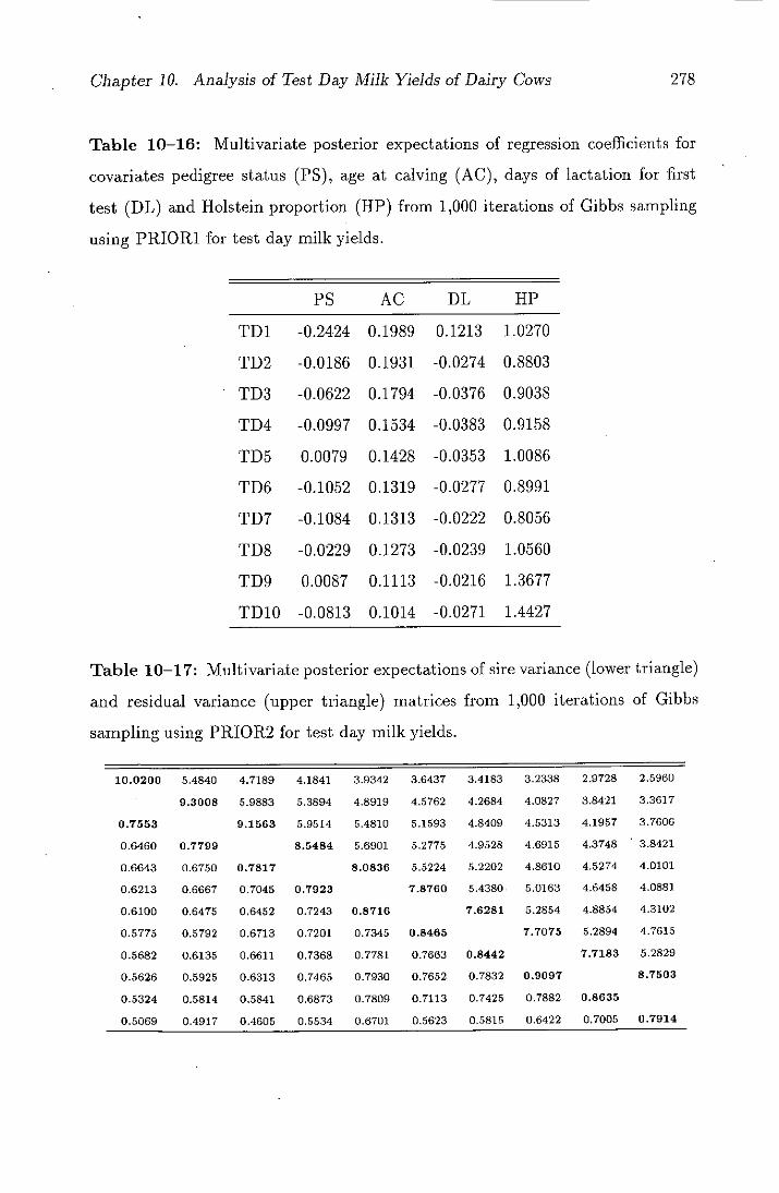
Chapter 10. Analysis of Test Day Milk Yields of Dairy Cows 278
Table 10-16: Multivariate posterior expectations of regression coefficients for
covariates pedigree status (PS), age at calving (AC), days of lactation for first
test (DL) and Holstein proportion (HP) from 1,000 iterations of Gibbs sampling
using PRIORI for test day milk yields.
PS AC DL HP
TD1 -0.2424 0.1989 0.1213 1.0270
TD2 -0.0186 0.1931 -0.0274 0.8803
TD3 -0.0622 0.1794 -0.0376 0.9038
TD4 -0.0997 0.1534 -0.0383 0.9158
TD5 0.0079 0.1428 -0.0353 1.0086
TD6 -0.1052 0.1319 -0.0277 0.8991
TD7 -0.1084 0.1313 -0.0222 0.8056
TD8 -0.0229 0.1273 -0.0239 1.0560
TD9 0.0087 0.1113 -0.0216 1.3677
TD1O -0.0813 0.1014 -0.0271 1.4427
Table 10-17: Multivariate posterior expectations of sire variance (lower triangle)
and residual variance (upper triangle) matrices from 1,000 iterations of Gibbs
sampling using PRIOR2 for test day milk yields.
10.0200 5.4840 4.7189 4.1841 3.9342 3.6437 3.4183 3.2338 2.9728 2.5960
9.3008 5.9883 5.3894 4.8919 4.5762 4.2684 4.0827 3.8421 3.3617
0.7553 9.1563 5.9514 5.4810 5.1593 4.8409 4.5313 4.1957 3.7606
0.6460 0.7799 8.5484 5.6901 5.2775 4.9528 4.6915 4.3748 3.8421
0.6643 0.6750 0.7817 8.0836 5.5224 5.2202 4.8610 4.5274 4.0101
0.6213 0.6667 0.7045 0.7923 7.8760 5.4380. 5.0163 4.6458 4.0881
0.6100 0.6475 0.6452 0.7243 0.8716 7.6281 5.2854 4.8854 4.3102
0.5775 0.5792 0.6713 0,7201 0.7345 0.8465 7.7075 5.2894 4.7615
0.5682 0.6135 0.6611 0.7368 0.7781 0.7663 0.8442 7.7183 5.2829
0.5626 0.5925 0.6313 0.7465 0.7930 0.7652 0.7832 0.9097 8.7503
0.5324 0.5814 0.5841 0.6873 0.7809 0.7113 0.7425 0.7882 0.8635
0.5069 0.4917 0.4605 0.5534 0.6701 0.5623 0.5815 0.6422 0.7005 0.7914
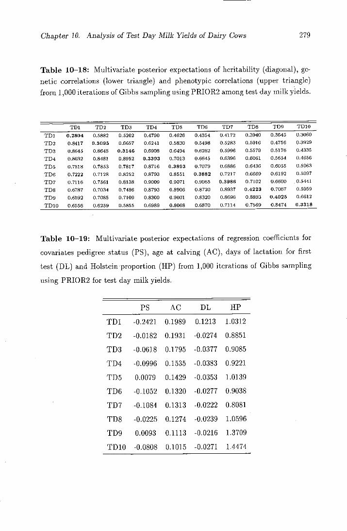
Chapter 10. Analysis of Test Day Milk Yields of Dairy Cows 279
Table 10-18: Multivariate posterior expectations of heritability (diagonal), ge-
netic correlations (lower triangle) and phenotypic correlations (upper triangle)
from 1,000 iterations of Gibbs sampling using PRIOR2 among test day milk yields.
TD1 TD2 TD3 TD4 TD5 TD6 TD7 TD8 TD9 TDIO
TM 0.2804 0.5882 0.5202 0.4790 0.4626 0.4354 0.4172 0.3940 0.3645 0.3060
TD2 0.8417 0.3095 0.6657 0.6241 0.5830 0.5498 0.5283 0.5016 0.4756 0.3929
TD3 0.8645 0.8645 0.3146 0.6908 0.6494 0.6262 0.5996 0.5579 0.5176 0.4335
TD4 0.8032 0.8481 0.8952 0.3393 0.7013 0.6645 0.6396 0.6061 0.5654 0.4656
TD5 0.7518 0.7853 0.7817 0.8716 0.3893 0.7079 0.6886 0.6436 0.6055 0.5063
TD6 0.7222 0.7128 0.8252 0.8793 0.8551 0.3882 0.7217 0.6669 0.6192 0.5097
TD7 0.7116 0.7561 0.8138 0.9009 0.9071 0.9065 0.3986 0.7102 0.6600 .0.5441
TDS 0.6787 0.7034 0.7486 0.8793 0.8906 0.8720 0.8937 0.4223 0.7067 0.5959
TD9 0.6592 0.7085 0.7109 0.8309 0.9001 0.8320 0.8696 0.8893 0.4025 0.6612
TD10 0.6556 0.6259 0.5855 0.6989 0.8068 0.6870 0.7114 0.7569 0.8474 0.3318
Table 10-19: Multivariate posterior expectations of regression coefficients for
covariates pedigree status (PS), age at calving (AC), days of lactation for first
test (DL) and Holstein proportion (HP) from 1,000 iterations of Gibbs sampling
using PRIOR2 for test day milk yields.
PS AC DL HP
TD1 -0.2421 0.1989 0.1213 1.0312
TD2 -0.0182 0.1931 -0.0274 0.8851
TD3 -0.0618 0.1795 -0.0377 0.9085
TD4 -0.0996 0.1535 -0.0383 0.9221
TD5 0.0079 0.1429 -0.0353 1.0139
TD6 -0.1052 0.1320 -0.0277 0.9038
TD7 -0.1084 0.1313 -0.0222 0.8081
TD8 -0.0225 0.1274 -0.0239 1.0596
TD9 0.0093 0.1113 -0.0216 1.3709
TD1O -0.0808 0.1015 -0.0271 1.4474

Chapter 10. Analysis of Test Day Milk Yields of Dairy Cows 280
high correlation between posterior expectations and REML estimates of breeding
values. Clearly, the two sets of predictions, and hence the rankings, are very
similar. Further a plot of average posterior expected breeding value versus the
number of unproven sires selected on 305-day lactation milk yield is illustrated
in Figure 10-2. In this figure, the continuous curve is obtained by sorting the
posterior expectations by themselves (BV1) and the dotted curve by sorting the
same expectations according to the REML estimates (BV2). Figure 10-2 indicates
that BV1 and BV2 methods of ordering reveal a slight difference between REML
and Bayesian ordering of sires.
Breeding values from multivariate analysis of test day records are obtained
giving equal economic weights to each trait, a' = [1 ... 1], and the results
are illustrated in Figures 10-3 to 10-7. Figures 10-3, 10-4 and 10-5 indicate
a roughly linear relationship between REML estimates and Bayesian posterior ex-
pected breeding values using different prior specifications PRIORI and PRIOR2
but with a lower correlation than in the univariate analysis. PRIOR2 gives slightly
higher expected breeding values than PRIORI. Figures 10-6 and 10-7 illustrate
plots of average posterior expected breeding values using PRIORI and PRIOR2
versus the number of unproven sires selected on ten test day records. In these
figures the continuous and dotted curves correspond to BV1 and BV2 as in the
univariate analysis. The dashed curve is obtained by sorting the posterior expected
breeding values using ten test day records by the posterior expected breeding val-
ues based on 305-day milk yield (BV3). The curves for BV2 and BV3 show the
expected reduction in progress from using REML estimates of breeding value and
from using only 305-day yield. The reductions appear similar for these two pro-
cedures.
A common feature in the plots of the expected versus estimated breeding values
resulting from univariate and multivariate analyses is that one of the unproven sires
gives an exceedingly high breeding value (see Figures 10-1, 10-3, 10-4 and 10-5).
This is investigated and it is found that the twelve daughters of the unproven

Chapter 10. Analysis of Test Day Milk Yields of Dairy Cows 281
sire number 535 consistently have high test day and 305-day lactation milk yield.
The means of the milk yields of the daughters are obtained for each of 11 traits
and these are compared with the overall mean of all the daughters of unproven
sires (Table 10-20). This particular sire has 87% Holstein proportion in his genes
while the mean Holstein proportion for all the proven sires is 42%. These findings
partly explain why the high yields for daughters of sire 535 leads to rather high
predicted breeding values. It would be useful to analyse the data without the
records of daughters of this sire.
Index weights: The vector of index weights corresponding to the mean vector
of family size ii is calculated using the REML estimate or posterior expectation
of the expression 2(nE 8 + E e ) -1 E3a. The values for some family sizes up to 20
are given for the REML and Bayesian methods in Table 10-21. In this table
the values of index weights for different methods are similar. The individual
weights for the first few test days with small family size are more variable due
to rapid changes in milk yield in the initial part of the lactation. In general, the
weights are low early in lactation, increasing gradually to the highest in month
5, they then decline irregularly. The index weights are mainly influenced by the
heritability of individual test days and genetic correlation among test day records.
The variation of index weights becomes less as the number of daughters per sire
increases, indicating that differences in heritability exert less influence on the
weights for large family sizes.
In the calculation of index weights, equal economic weights are given to each
trait. Economic weights could alternatively be determined according to the value
of increased milk yield in different phases of the lactation.
10.7.4 Canonical variables
As discussed in Chapters 8 and 9, the canonical transformation in a multivariate
analysis involves finding the eigenvalues and eigenvectors of the genetic variance

Chapter lii. Analysis of Test Day Milk Yields of Dairy Cows 282
—J
Ui
U, C, = 0, C
-o C, C,
-0 -D a, C,
E U, Ui
-500 0 500 1000 1500
Posterior expected breeding values (Gibbs)
Figure 10-1; Bayesian posterior expected breeding values versus REML esti-
mates of breeding values for 305-day lactation milk yield.
Co a, = 0, C
-D 0 0,
-0
-o 0, U 0 0- x 0 0 0) a, 0
0 100 200 300 400 500 600
Number of sires selected
Figure 10-2: Plot of average posterior expected breeding values against the
number of unproven sires selected using 305-day lactation milk yield. ( ), sires
ranked by expected breeding values (BV1); (.....), sires ranked by REML
estimates (BV2).

Chapter 10. Analysis of Test Day Milk Yields of Dairy Cows 283
—J
Lu It
0 0 = 0) C
-c 0 0 -0
0
c0 E 0,
Lu
-20 -10 0 10 20 30
Posterior expected breeding values (Gibbs)
Figure 10-3: Bayesian posterior expected breeding values versus REML esti-
mates of breeding values for test day records with equal weights using PRIORI.
—J
w It
C" 0 = 0) = 0 0
-0
0
Ce E C, Ui
-20 -Ia 0 10 20 30
Posterior expected breeding values (Gibbs)
Figure 10-4: Bayesian posterior expected breeding values versus REML esti-
mates of breeding values for test day records with equal weights using PRIOR2.

Chapter 10. Analysis of Test Day Milk Yields of Dairy Cows 284
c'J
0 It 0-
0 0
CD > 0) C V 0 0 n V 0
0 0. x 0
0 = 0 L0 0 0-
-20 -10 0 10 20 30
Posterior expected breeding values (PRIORI)
Figure 10-5: Bayesian posterior expected breeding values for test day records
using two priors, PRIORI and PRIOR2.
0, 0 =
a, C
0 2 -0 0 0
0
0 0 0 CO 0 >
0 100 200 300 400 500 600
Number of sires selected
Figure 10-6: Plot of average posterior expected breeding values against the
number of unproven sires selected using ten test day milk yields and PRIORI.
( ), sires ranked by expected breeding values (BV1); (.....), sires ranked by
REML estimates (BV2); (-----), sires ranked by the posterior expected breeding
values using 305-day milk yield (BV3).

Chapter 10. Analysis of Test Day Milk Yields of Dairy Cows 285
0 U,
CU > 0, C
-D 0
8 .0 -D 0
0 0-'C 0
0 0 CU
0
0 100 200 300 400 500 600
Number of sires selected
Figure 10-7: Plot of average posterior expected breeding values against the
number of unproven sires selected using ten test day milk yields and PRIOR2.
), sires ranked by expected breeding values (BV1); (.....), sires ranked by
REML estimates (BV2); (-----), sires ranked by the posterior expected breeding
values using 305-day milk yield (BV3).
matrix relative to the phenotypic variance matrix, that is the solutions A 1 , . . . , At
of I Eg - 0. Apart from being a powerful statistical tool in reducing the
computational requirements, it has an interpretation in its own right. It yields
canonical variables which are both genetically and phenotypically uncorrelated
and have unit phenotypic variance. Furthermore, the canonical variable with the
kth largest eigenvalue, or equivalently heritability, explains the maximum amount
of genetic variation given the k - 1 canonical variables with larger eigenvalues
(Hayes and Hill, 1980). Meyer (1985) examined the canonical variables resulting
from a multivariate analysis of first lactation milk, fat and protein yields.
In this chapter, a different approach is taken to presenting canonical variables
Gibbs sampling provides 1,000 samples from the joint distribution of E,, and E 9 ,
and hence 1,000 sets of values of the canonical roots A 1 ,..., A10 . The cumulative

Chapter%10. Analysis of Test Day Milk Yields of Dairy Cows 286
Table 10-20: Raw means of daughters of all the unproven sires and of sire
number 535.
Mean of daughter of Mean of daughters of Trait all the unproven sires sire 535
TIll 19.43 20.92
TD2 20.68 23.37
T133 19.71 24.95
TD4 18.61 25.38
TB5 17.61 24.48
TD6 16.78 22.87
TD7 16.19 22.72
TD8 15.60 21.65
T]J9 14.70 21.65
TB10 12.94 18.72
LMY 5268.80 6936.77
distribution functions of these roots are then plotted together. If the genetic
variation in test day yields is the result of only a few underlying factors and these
act linearly on the genetic components of the records, then we expect to find that
a few of the roots are large and the rest are relatively small. Figure 10-8 a) and
b) illustrates these distribution functions for PRIORI and PRIOR2. From this
diagram it can be seen that there is not a clear grouping of canonical variables,
except that the largest appears substantially larger than the rest. They all seem
to contribute to the genetic variation.
10.8 Discussion
In this chapter, we have demonstrated the feasibility of the Gibbs sampler to
handle a relatively large data set in unbalanced univariate and multivariate half-sib
sire models. We found that for this particular data set, the posterior expectations
from the Gibbs sampling and the REML estimates are fairly similar. Herd-year-

Chapter 10. Analysis of Test Day Milk Yields of Dairy Cows
287
Table 10-21: Index weights corresponding to means of different family sizes for
REML and Bayesian methods.
ii b, b2 b3 54 b5 b6 b7 b8 bg blo
REML
1 0.225 0.227 0.233 0.250 0.266 0.247 0.253 0.261 0.256 0.231
2 0.201 0.203 0.208 0.222 0.236 0.219 0.224 0.231 0.227 0.205
3 0.182 0.183 0.188 0.200 0.211 0.197 0.201 0.207 0.204 0.184
4 0.167 0.167 0.171 0.182 0.192 0.178 0.183 0.188 0.185 0.168
5 0.153 0.153 0.157 0.167 0.176 0.163 0.167 0.172 0.169 0.154
10 0.110 0.110 0.112 0.118 0.123 0.115 0.117 0.120 0.119 0.109
15 0.086 0.085 0.088 0.091 0.095 0.088 0.090 0.092 0.091 0.084
20 0.071 0.070 0.072 0.074 0.077 0.072 0.073 0.075 0.074 0.069
PRIORI
1 0.222 0.223 0.222 0.240 0.254 0.243 0.246 0.251 0.248 0.232
2 0.199 0.200 0.199 0.214 0.226 0.217 0.219 0.224 0.221 0.206
3 0.181 0.181 0.180 0.193 0.204 0.195 0.198 0.201 0.199 0.186
4 0.165 0.165 0.165 0.176 0.185 0.178 0.180 0.183 0.181 0.169
5 0.152 0.152 0.152 0.161 0.170 0.163 0.165 0.168 0.166 0.155
10 0.110 0.109 0.109 0.115 0.120 0.116 0.117 0.118 0.117 0.110
15 0.086 0.086 0.085 0.089 0.092 0.090 0.091 0.091 0.091 0.086
20 0.071 0.070 0.070 0.073 0.075 0.073 0.074 0.074 0.074 0.070
PRIOR2
1 0.222 0.223 0.226 0.244 0.259 0.244 0.248 0.255 0.252 0.226
2 0.199 0.199 0.202 0.217 0.230 0.217 0.221 0.226 0.223 0.202
3 0.180 0.180 0.183 0.196 0.207 0.195 0.198 0.203 0.201 0.182
4 0.165 0.165 0.167 0.178 0.188 0.178 0.180 0.185 0.182 0.166
5 0.152 0.152 0.154 0.164 0.172 0.163 0.165 0.169 0.167 0.152
10 0.110 0.109 0.110 0.116 0.121 0.115 0.116 0.119 0.118 0.109
15 0.086 0.085 0.086 0.090 0.093 0.089 0.090 0.091 0.091 0.085
20 0.071 0.070 0.071 0.074 0.076 0.073 0.073 0.074 0.074 0.070

Chapter 10. Analysis of Test Day Milk Yields of Dairy Cows 288
C 0
C = C 0
= -0
0 •0 0 > cc = E =
C)
0.0 0.1 0.2 0.3 0.4 0.5 0.6 0.7 0.8 0.9 1.0
Canonical heritabilities
REML : 0.000, 0.000, 0.000, 0.000, 0.048, 0.083, 0.139, 0.239, 0.302, 0.515
a)
C 0
C
= 0 0 n = C0 V 0
cc = E 0
C)
0.0 0.1 0.2 0.3 0.4 0.5 0.6 0.7 0.6 0.9 1.0
Canonical heritabilities
b)
Figure 10-8: Plot of posterior expectations of canonical heritabilities versus cu-
mulative distribution functions for test day milk yields using two different prior
specifications, a) PRIORI and b) PRIOR2. REML estimates of canonical hen-
tabilities are given between two graphs.

Chapter 10. Analysis of Test Day Milk Yields of Dairy Cows 289
month effects should be treated as fixed rather than random (or, from a Bayesian
perspective, we should put uniform priors on them) because of the potential bias
in the information contained in between herd-year-month comparisons. The type
of analysis based on a model that treats herd-year-month effects as random is
included to demonstrate how the Gibbs sampler can be applied to a more complex
model. In this section, the results from the univariate analysis of the model (10.2)
and multivariate analysis of the model (10.29) will be mainly discussed.
Co variates: The effect of age at calving decreases towards the end of lactation
which is also found by other studies (Auran, 1973; Danell, 1982a; Pander et al,
1993). This indicates that the heifers are gradually maturing towards the end of
the lactation. Days of lactation for first test has the highest effect on the first test
day. This may be due to rapid changes in milk yield during early lactation.
Heritabilities: In all cases, the heritabilities for the individual test days are
lower than for the corresponding 305-day lactation yield. The heritability esti-
mates obtained from using REML and Gibbs sampling procedures in univariate
and multivariate analyses are higher than those previously reported, but the pat-
tern across test day is similar to published reports (see Table 10-2). Pander et al.
(1993) have given a set of reasons for high heritabilities. Some of these are:
the use of different models (models with herd-year-month effects or with
herd-year-season effects),
data sets collected in different years and countries and even different regions
within a country, and
different types of data (i.e. data on daughters of bulls from a progeny testing
scheme or from non-progeny testing scheme).
These reasons are not investigated in the present study. Pander et al. (1993) have
looked into the reasons behind high heritability estimates. A significant difference

Chapter 10. Analysis of Test Day Milk Yields of Dairy Cows 290
between the data set used in this study and previous studies is that the present
data come from a recent year representing 7,973 herds, whereas in others data span
many years and represent a various numbers of herds, ranging from 100 to 4,000.
Estimates or posterior expectations of higher heritability in this study may also
be due to lower environmental variance owing to fitting herd-year-month rather
than herd-year-season effects as in other studies. High heritabilities coincide with
increase in sire variance component. Lower heritability estimates in the early part
of the lactation are due to both a relatively low sire variance component and a
high residual variance component.
Genetic and phenotypic correlations: The estimates of genetic and phenotypic
correlations between test day milk yields are in good agreement with the literature
results. In general, the phenotypic correlations are lower than the genetic correla-
tions. Both correlations are higher during the mid lactation than at the beginning
and at the end of lactation. The highest correlations are obtained for consecutive
test days, but as the intervals between test days increase the correlations decrease.
Sire evaluation: Evaluation of sires in the dairy industry is traditionally based
on 305-day lactations, and changing to a system of genetic evaluations using indi-
vidual test day milk yields may be resisted. However, the lactation milk yield used
for evaluations is not the actual 305-day lactation milk yield; it is a predicted yield
which may be biased in contrast to test day milk yields which are actual yields.
In this time of easy access to computer power and implementation of rather com-
plicated models for genetic evaluations, more accurate selection decisions can be
made by using breeding values from test day milk yields rather than from the
predicted phenotypic yields.
As discussed before, the results of univariate and multivariate analyses show
that heritability is lowest in early lactation and the genetic correlations are not
very high. But from test day 3 onwards the genetic correlations and heritabilities
get higher. Several authors (Danell, 1982a; Wilmink, 1987; Pander et al., 1993)

Chapter 10. Analysis of Test Day Milk Yields of Dairy Cows 291
have warned against too much consideration on the first test day for the early
selection decisions as the unexplained part of the total variance for this test day
is highest. Indeed the accuracy of indirect selection on a few tests would be less
than direct selection based on the complete lactation. This loss in accuracy can be
compensated by increased selection intensity. Therefore selection on early test may
become more advantageous if one considers the reduction in generation interval.
The overall conclusion is that with test day models, substantial improvements over
models based on 305-day lactation milk yield can be made, and test day models
offer the opportunity of a more flexible system of evaluation. It is also observed
that when Bayesian methods are used there is a scope for genetic improvement
over the REML method.
Computing considerations: The traditional computer requirements of a mul-
tivariate analysis is generally due to increased number of equations to be solved.
Changing from a univariate 305-day genetic evaluation system to a multivariate
test day evaluation system will require the storage and processing of individual
test day milk yields. In such a change over, the number of records to be pro-
cessed per iteration of Gibbs sampling in a multivariate analysis increases by a
factor of ten due to more factors being included in the models which require more
memory space and more iteration, and presumably processing cost would also in-
crease ten-fold. For example, a univariate Gibbs sampling analysis of each test
day or 305-day milk yield takes about 17-18 hours to perform 1,000 iterations
on a Sun Sparcstation 5 while a multivariate analysis of ten test day milk yields
takes slightly more than 7 days. Although this seems a huge amount of time,
it accounts for a small proportion of the total costs when one considers all costs
of data preparation, updating pedigrees and names, editing, sorting, and so on.
A ten-fold increase in costs of the genetic evaluation portion may therefore not.
be critical. The use of supercomputers employing parallel programming would
dramatically reduce the time taken for the genetic evaluations.

Chapter 11
General Conclusions and Future Work
11.1 Conclusions
The Bayesian approach to statistics offers a self-consistent theory for inference,
prediction and decision making which can incorporate prior information on model
parameters and on the utilities associated with different decisions. As such, it
appears applicable to inferences from animal breeding data and to decisions such
as which animals to select for breeding and that traits to measure in a breeding
programme. Until recently, the lack of adequate computing power and the absence
of suitable algorithms have prevented the use of this approach in realistic problems.
Where it has been used, the emphasis has been on obtaining point estimates rather
than genuine decision problems.
The purpose of this thesis is mainly to provide quantitative geneticists and an-
imal breeders with algorithms demonstrating how Gibbs sampling can be applied
to inferences and decision making in animal breeding in univariate and multivari-
ate sire models assuming a half-sib family structure. Discussions in the literature
on the use of multivariate procedures for continuous data indicate two reasons for
the superiority of multivariate over univariate analyses. Multiple-trait procedures
use more information to evaluate individuals and are able to remove bias due to
selection on a correlated trait, provided that records on which selection was based
are included in the analysis. The gain in accuracy of selection due to multivariate
292
Chapter 11. General Conclusions and Future Work 293
evaluations depends on the absolute values of genetic and residual correlations and
on progeny group size. Further, the superiority of multiple-trait procedure can be
dissipated if incorrect genetic and residual variance matrices are used. Conven-
tional procedures based on point estimation become less satisfactory as more traits
are incorporated. Therefore there is an increasing need for a consistent approach
to inference and decision making in animal breeding.
The iterative Gibbs sampling procedure provides a means to obtain the marginal
distributions of model parameters without using complicated numerical integra-
tion procedures. It turns an analytically intractable multidimensional integration
problem into a feasible numerical one. Application of the Gibbs sampling pro-
cedure to animal breeding data will contribute to a better knowledge of genetic
properties of the traits. The Bayesian methods using this approach have many
advantages over the conventional procedures and some of these will be given here.
Gibbs sampling is relatively straightforward to implement. Given the likeli-
hood function and the prior distribution, one can always obtain the joint posterior
density of all the unknown parameters of interest. From this density function, at
least in the normal linear model one can directly get the full conditional distribu-
tion of a particular parameter given the remaining parameters in the joint posterior
distribution. The set of all full conditional densities gives the expressions needed
for implementing the Gibbs sampler. The full conditional densities in this case
are in families of distributions, such as normal and inverse-x 2, where generating
random variables is not exceedingly complicated. -
Bayesian prediction procedures provide an appealing alternative to the REML
and other frequentist procedures. One of the potential advantages of the Bayesian
procedures is that they provide a formal mechanism for incorporating prior infor-
mation about the variance components in univariate and multivariate analyses.
This prior information is often available, and can be obtained from the results of
similar studies, or animal breeders' opinions about the likely values of parameters.

Chapter 11. General Conclusions and Future Work 294
Moreover the Bayesian procedures implicitly account for the uncertainty about
the values of variance components and selection responses; the methods such as
REML developed within the conventional framework for accounting for this un-
certainty tend to be rather ad hoc and do not always produce sensible answers.
For example, the results from the simulation study in Chapters 7 and 9 indicate
the power of Bayesian analysis to reveal uncertainty in response to selection when
the information contained in the data about the appropriate parameters is small.
Depending on the choice of prior distribution, the Bayesian procedures may have
appeal from a frequentist perspective.
As Bayes theorem operates within the parameter space, all statistics fall within
permissible ranges. For example, in the univariate analysis of the sire model,
the posterior expectations of variance components a 2 and a can be thought of
as averages of a finite number of Gibbs sampling iterations. This ensures that
Bayesian point estimates of variance components will always be within the per-
missible parameter space. This is a serious problem of conventional procedures
such as ANOVA and REML. Although the REML estimates are defined within the
permissible parameter space, interval estimates based on asymptotic theory can
include negative values. The use of such estimates in the construction of selection
indices can lead to very inefficient selection decisions. Therefore, point estimation
of variance components is not required for selecting animals. Theobald (1994)
point this out but does not implement a Bayesian procedure.
It has been illustrated that the Bayesian marginal inferences are robust to
changes in the prior specifications. When the amount of information contained
in the data is adequate, inferences are affected little by the choice of priors. It is
not generally a simple matter to decide when one has adequate information, and
it may be therefore necessary to carry out analyses with different priors to study
how inferences are affected. If use of different priors leads to very different results,
this indicates that the information in the likelihood is weak and more data ought
to be collected in order to draw firmer conclusions. Theoretical considerations as

Chapter II. General Conclusions and Future Work 295
well as empirical evidence suggest that the Bayesian posterior expectations present
an advantage over the estimates obtained from an conventional method when the
data contain little information about the unknown variance components regardless
of the choice of priors. In this case, point estimates of variance components may
be highly variable.
Harville (1990) obtained genetic and phenotypic parameters and functions of
them from a small data set using the conventional and Bayesian methods. He
found that the conventional method was highly dependent on the ratio between
the sire and residual variances. Further he observed that a relatively small change
in the data produced a large change in the conventional estimates, but not in the
Bayesian posterior expectations. This indicates that the Bayesian approach may
produce results which are more robust to changes in the data than the conventional
methods. This can perhaps be explained by the fact that changes in the data
may produce a large change in the point estimate of variance parameters, but a
relatively small change in their posterior distribution.
The Bayesian approach may produce more reliable predictions than the con-
ventional approach in cases where it is desired to perform a simultaneous analysis
of more than one trait. For a given amount of data, the larger the number of
variances and covariances to be estimated, the poorer those estimates are. This
may be more pronounced in the case where information on traits is missing on
some individuals.
Gibbs sampling enables posterior joint and marginal distributions of interest
to be constructed, in principle to any degree of accuracy. Thus the Gibbs sam-
pling approach to prediction of the random-effects sire model does not suffer from
approximations or deficiencies inherent in other approaches, notably the ANOVA
and REML procedures. Moreover, having available full posterior distributions in-
stead of normal approximations to them can be valuable, particularly for highly
skewed posteriors where maximum a posteriori estimates are misleading (Gilks et

Chapter 11. General Conclusions and Future Work 296
al., 1993). The Gibbs sampling approach also allows posterior distributions to
be easily calculated for arbitrary functions of parameters such as variance ratios,
heritabilities and selection responses.
Another major advantage of the Gibbs sampling approach is its flexibility.
That is, particular features of a given set of data can be accommodated with only
minor changes to the set of full conditional distributions. This was demonstrated
in Chapter 10 with the analysis of test day milk yields employing different models,
one treating herd-year-month effects as fixed and another as random. This feature
of Gibbs sampling also allows posterior distributions to be easily calculated for
arbitrary functions of the original parameters such as variance ratios, canonical
heritabilities and selection responses, using standard theory of random variable
transformation, with minimal calculations.
However, a disadvantage of Gibbs sampling is that it is computationally more
demanding than the conventional methods. The demand is in terms of computer
time rather than in terms of programming complexity. This certainly limits the
applicability of the procedure, at least at present. For example, in the multivariate
analysis of test day milk yields from 23,873 daughters of 689 sires in Chapter
10, the Gibbs sampler took about 8 days to perform 1,000 iterations on a Sun
5 Sparcstation, whilst the REML program produced results in only 5 minutes.
Although relatively this seems a huge disadvantage, in absolute practical terms in
a multitasking computer environment it makes little impact, and relative to the
time taken to collect the data (over many years) it is irrelevant. Application of
the Gibbs sampling procedure may therefore depend on the availability of very
fast computers (parallel processing) for large data sets and of sufficiently accurate
routines for random number generations. With current advances in computer
technology, it is likely that much larger models could be handled efficiently in the
near future.

Chapter 11. General Conclusions and Future Work 297
11.2 Extension of the work
One possible extension of the Gibbs sampling methodology would be to generalised
linear random-effects models or threshold models where discrete phenotypes are
modelled as having an underlying distribution which is continuous. So long as
conjugate priors can be found for model parameters, application of the Gibbs
sampling methodology is straightforward, as illustrated in Chapters 4, 7, 8, 9 and
10. For generalised linear models, conjugate priors will not in general be available,
and sampling from the complex full conditional distributions that arise might be
problematical. When a convenient envelope function to the density can be found,
rejection sampling can be used. Zeger and Karim (1991) have recently proposed a
method for Gibbs sampling for generalised linear models with random effects by
rejection sampling from multivariate envelopes. Alternatively, adaptive rejection
sampling might be used (Gilks and Wild, 1992) for sampling from univariate
log-concave full conditional distributions. An application of adaptive rejection
sampling to the analysis of a random sire model in animal breeding is given in
Chapters 6. Dellaportas and Smith (1993) show that full conditionals are always
log-concave for generalised linear models with canonical link.
Gelfand et al. (1990) illustrated how the Gibbs Sampler deals with compli-
cations arising from missing data in a crossover trial. They reported that the
Gibbs Sampler provides predictive densities for missing responses. The methodol-
ogy developed in this thesis can be extended to the cases in which information on
some traits is missing on some individuals. The feasibility of the Gibbs sampling of
procedure enables the analysis data sets with missing observations.
Throughout this thesis a half-sib family structure has been used in making
inferences about genetic and phenotypic parameters and constructing selection
indices. It is possible to use different family structures. One could study the
design of selection experiments. Using the procedures developed here, a variety of

Chapter 11. General Conclusions and Future Work 298
designs could be examined and their efficiency compared by means of analyses of
predictive distributions.
Further research is required into the repeated-measures aspect of test day
records (except in PRIORI), i.e. a kind of time-series model relating measure-
ments at successive times. This would involve parametric structure for E, and
Ee and maybe for the expectations (a model for the lactation curve). An appro-
priate model should lead to more precise inferences about parameters and better
selection decisions.
Gibbs sampling has enormous potential for analysing complex data sets. How-
ever, the utility of Gibbs sampling has been hampered by the lack of general
purpose software for its implementation. A purpose-built program is required for
Bayesian inference, prediction and decision-making in animal breeding, at least
for Normal models. The main requirements of such a program should be that it
accommodates a very large class of models, deals with missing values, provides
assistance with specifying prior distributions as well as examination of posterior
distributions and produces summary statistics, marginal posterior expectations
and standard deviations.

Appendix A
Notes on Various Distributions
The material in this appendix contains distributions which are used throughout
the thesis. Some of which were used as priors in Chapter 4, 6 and 10, for instance.
Most of them were used in simulation studies. Each of the distribution is defined
by a density function, and some of their properties are outlined.
A.1 The Generalized Beta Distribution
If a random variable X has a density given by
(b - a) f(x) = Ax I ,/3)
= B(a) —a) (b—x) , a <x <b, (A.1)
where c > 0 and 0 > 0, then X is defined to have a generalized beta distribution.
This distribution is denoted as Beia(a,8;a,b), and a mean and a variance are.
ace a +bfl = and Var(X) =
(b -
ao ___ __ ( a +/3+l)(a+fl)2
Beta(a, 0; 0,1) is a usual beta distribution, and furthermore Beta(1, 1; a, b) is
a uniform distribution in a range [a, b]. Since the former two parameters a and 0 are related to a shape of this distribution, they are called shape parameters, and
the latter two parameters a and b are called range parameters for the same reason.
The function Beta(a,B) = f' x(1 - x)' 1 dx, is called the beta function.
299

Appendix A. Notes on Various Distributions KIID]
A.2 The Chi-square and Inverse Chi-square Dis-
tributions
If X is a random variable with probability density function
(x)_1 exp (-) f(x v) = x>O, - (A.2)
then X defined to have a x 2 distribution with v degrees of freedom. It can be shown
that E(X) = t', and Var(X) = 2v. In the Bayesian analysis, it is the reciprocal
X 1 which naturally appear. The inverse x2 distribution having v degrees of
freedom is derived from (A.2) by making the transformation X 1 = 11X, to yield
(x_1)1 exp (_x1) > 0. (A.3) f(x v)=
22
Now comparing the prior distributions in (4.5) and (4.6) for a 2 and a, respectively,
with (A.3), we see that a priori the quantities o,, 21V,3 and a/v6 are distributed
as X'. In dealing with the prior distributions of such quantities as a/v3 s and
a/ve s, it must be remembered that a and a are the random variables and s
and s are fixed quantities.
A.3 The Univariate Normal Distribution
A real random variable X is defined to have a normal distribution with mean ji
and precision a if its density is given by
exp- _____
2a2 ' °°<<°° (AA)
where the parameters i and a satisfy —oo <x <oo and a> 0. This relationship
is denoted by X N(jt,a2).

Appendix A. Notes on Various Distributions 301
A.4 The Univariate Student-t Distribution
If X is a random variable having density given by
1 1 - <x < , (A.5)
Do f(x v) -
r() (2\4(V+fl'
then X is defined to have a student-t distribution with v degrees of freedom. It
can be shown that
E(X)=0, v>1, and \Tar(X)= 11
v>2.
A.5 The Multivariate Normal Distribution
A p-dimensional random variable X follows the multivariate normal distribution
if its joint probability density function is of the form
f(x ,E)= 2 exp --(x—p)'E-
- 1(x )
1 }
(A.6) (21r)2(5 2
where S is any (p x p) symmetric positive definite matrix. Moreover, if X 1 ,.. . , Xp
are independent random variables where X N1 (jt, cf), then their joint proba-
bility density function is simply the product of the appropriate (marginal) density
functions, so that
1 f(xi,.
exp{_ ]2}. (A.7) . . ,x =
(2 a R-)2 fl1 'i
2 i=1
In this case X = [X 1 . . . Xi,] has mean = [ji . . . ps,] and covariance matrix S.
But of course the components of X do not generally need to be independent and
so S does not have to be diagonal, provided that it is symmetric and positive
definite. The requirement that S be positive definite can be thought of as the
multivariate equivalent of the condition that a 2 > 0 in the univariate case. It is

Appendix A. Notes on Various Distributions 302
clear that f(x) > 0 for every x and it is also straightforward, though algebraically
tedious, to check that f, f(x)dx i ... dx i, = 1 for every p and for every E which.
is symmetric and positive definite. After some algebra, it is also possible to show
that E(X) = p and that E is the covariance matrix for x. Thus the parameters
p and E have an immediate interpretation, and we write X N(p, ), where
p denotes the dimension of X, p denotes the mean vector and E denotes the
covariance matrix. The definition of the multivariate normal distribution via the
equation above also requires the covariance matrix to be non-singular so that E'
exists.
A.6 The Wishart Distributions
A.6.1 The Wishart and inverse Wishart distributions
Let X be a p x p positive definite symmetric random matrix which consists of
p(p + 1) distinct random variables xjj (i,j = 1,...,p; i > j). Let v > p, and
be a p x p positive definite symmetric matrix of fixed constants. The distribution
Of Xij
f(X v,E) = X exp (_trE_1x), X > 0 (A.8)
is a multivariate generalization of the x2 distribution where
= 2 E F and F () = r+_1) ñ [i(v + 1 - i)] P(P i=1
(the so-called multivariate gamma function). The distribution (A.8) is denoted by
W(E, ii) and is said that X is distributed as Wishart with v degrees of freedom
and parameter matri* E.
If p = 1 and E = 1, the Wishart density becomes that of the chi-squared
distribution with '.' degrees of freedom given in (A.2).

Appendix A. Notes on Various Distributions 303
The inverse Wishart distribution can be obtained by taking the inverse of X
matrix and using the Jacobian. Let x" denote the (i,j)ih element of the inverse
of X Then the Jacobian of the transformation of the !p(p + 1) random variables
(xii ,x12 ,. . , x) to (x 11 ,x 12 ,...
Is 3(x11,x12,. .,x)i = p+i
3(x 11 , x' 2 , . . , x")
Consequently, the probability density function of the inverse Wishart distribution
is
v, E) cc X +1) exp (_trx_1E), I X I> 0. (A.9)
The distribution of X in (A.9) may thus be called an p—dimensional inverse
Wishart distribution with v degrees of freedom, and be denoted by WP-1 (E,
Here E and ii are called hyperparameters.
Note that when p = 1 the distribution in (A.9) reduces to an inverse x2
distribution in (A.3). When in (A.9) X is a scalar, say x 11 , the probability density
function for x 11 is
1v-f-2) 7 a11 \
cc exp -) , x 11 > 0.
By letting, for example, a 2 = x 11 and o- 11 = v 8s, the inverse x2 distribution for
can be obtained
(vs+2) (
38\ 2 f(o v, s) cc (a)
exp ----) , as > 0,
which is the prior distribution of a given in (4.5).
A.6.2 The Wishart random variate generation
The Wishart distribution is one of the few multivariate distributions for which
computer generation algorithms are not widely available. Outside the normal

Appendix A. Notes on Various Distributions D7iI
distribution theory framework, the Wishart distribution has united appeal. Hence,
in this section attention focuses on the variate generation of this distribution.
A p x p symmetric matrix X has a Wishart distribution with parameters E,
ii and p and denoted W(E, ii). The standard procedure for generating random
variates from the Wishart distribution (Johnson, 1987) is as follows. Let I be a
lower triangular p x p matrix with entries Tij satisfying:
Tjj is standard normal for i > j
Ti i
Tjj 's are independent.
The matrix X = TI' has a W(I, 'j') distribution. Handling a matrix other than
the identity matrix is easy. Let the p x p symmetric matrix E have the standard
Choleski decomposition, E = LL', with L lower triangular matrix, so ljj > 0,
Iij = 0 if j > i. Then Y = (LT)(LT)' = LTT'L' = LXL' has a W. (E, ii)
distribution. The p x p matrix LT and the result can be efficiently computed
using the triangular properties of L and I.

Appendix B
The Likelihood Functions
B.1 The Likelihood Function of (ii, a, ) for Half-
sib Analysis
From distributional assumptions of multivariate normality for the Yji, it is possible
to find the likelihood function for a families of size it. For jih member of family i
the model is
yij = +s+ei i = 1,...,s; j = l,...,n, (B.1)
where observations, Vii, on the members of families of equal sizes of h are obtained
from the simulation program, s N(O, a) and N(O, U 2 ). If s i 's and e's
are all independently distributed then the probability density function of {yj}
given (p,{sj},o,o) is
I {s}, 0'. , c) () 1 1 FE E(y3 - - S i )
} 2 U2
(B.2)
and the probability density function of {s} given (p, as ) o) is
2 58 1 1 ~""l )f({s} I t,c,c) (cry ) exp—
2 il• (B.3)
To obtain f({yj} ji, o- , o), we may integrate out the s from the product
of (11.2) and (11.3), or note that the vector of observations for the ith family,
Yi = [YiI Yu2 Yin] ' , has multivariate normal distribution with mean vector [tin
305
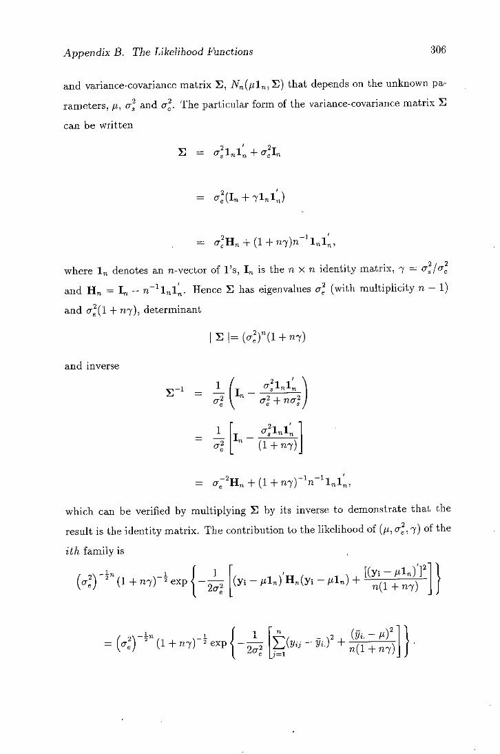
Appendix B. The Likelihood Functions 306
and variance-covariance matrix E, Nn (tin, ) that depends on the unknown pa-
rameters, p, cx and cr. The particular form of the variance-covariance matrix Y
can be written
= ai fl i fl + a 21n
= a(In +71ni)
21 1l = Ole H. + (1 + n7)n 1 n 1,
where In denotes an n-vector of l's, In is the it x it identity matrix, -y =
and ll = - 7-1j' Hence E has eigenvalues a (with multiplicity it - 1)
and o,, 2(l + n7), determinant
(a(1 +
and inverse
= (in_ aii,\
or 2 c + nat)
- 4 [In
1 -
= a 2 11 + (1 + n-y) 1 n'1m 1,
which can be verified by multiplying E by its inverse to demonstrate that the
result is the identity matrix. The contribution to the likelihood of (t,cy) of the
ith family is
1 1 + KYi _ P 1 n )I 2 1l () -4 (1 + exp {-
[(Yi - M m) Hn (yi - Mi) it(1 + n7) j 5
( M ) 2 l = ()± (1 + exp {
It1 - v.)2 + n(l + n)j f

Appendix B. The Likelihood Functions 307
Hence the likelihood of (p, o, 'y) for all .s families is
f({yjj} p,a) OC
(
0, 2) -2 6
x exp {_J_ [sw
+ nY7=1(7i. - 1t) 2 1) 2c 1+927
nothing that
- = nS
- y.3 2 + sn( -
= Sb+ns(. p)2
2 2 2 (1 +
f({yj} p, c6,7) (0, 2)
X exp ~ _ I [S. + Sb + nS(Y.. —
/1)2
1+927 j
where
Sb
= -
S IL
SW = YL( -)2
1=1 j=1

References
Anderson, T.W. (1984) An Introduction to Multivariate Statistical Analysis, Wi-
ley, New York.
Auran, T. (1973) Studies on monthly and cumulative monthly milk yield records.
I. The effect of age, month of calving, herd and month of first period. Acta
Agric. Scand., 23, 189-199.
Auran, T. (1976) Studies on monthly and cumulative monthly milk yield records.
III. Estimates of genetic and phenotypic parameters. Acta Agric. Scand., 26,
3-9.
Berger, JO. (1985) Statistical Decision Theory. Springer-Verlag, New York.
Bernardo, J.M. and Smith, A.F.M. (1994) Bayesian Theory. John Willey and
Sons, New York.
Besag, J. (1974) Spatial interaction and the statistical analysis of lattice systems
(with discussion). J. Roy. Statist. Soc. Ser. B, 36, 192-326.
Besag, J., York, J.C. and Mollie, A. (1991) Bayesian image restoration, with two
applications in spatial statistics (with discussion). Ann. Inst. Statist. Math.,
43, 1-59.
308

References I 309
Blair, H.T. and Pollak, E.J. (1984) Estimation of genetic trend in a selected pop-
ulation with and without the use of a control population. J. Anim. Sci., 58,
878-886.
Box, G.E.P. and Tiao, C.C. (1973) Bayesian Inference in Statistical Analysis.
Addison-Weiley, Reading.
British Standards Institution. (1972) Recommendations for the methods of milk
recording of cows. British Standards Institution 4866, 12-17.
Broemeling, L.D. (1985) Bayesian Analysis of Linear Models. Marcel Dekker, New
York.
Campbell, N.A. (1980) Shrunken estimators in discriminant and canonical variate
analysis. Appi. Statist., 29, 5-14.
Cantet, R.J.C., Fernando, R.L. and Gianola, D. (1992) Bayesian inference about
dispersion parameters of univariate mixed models with maternal effects: The-
oretical considerations. Genet. Sel. Evol., 24, 107-135.
Clayton, D.C. (1991) A monte carlo method for Bayesian inference in Frailty
models. Biometrics, 47, 467-485.
Cox, D.R. and Reid, N. (1987) Parameter orthogonality and approximate condi-
tional inference. J. Roy. Statist. Soc. Ser. B, 49, 1-39.
Crump, S.L. (1951) The present status of variance component analysis. Biomet-
rics, 7, 1-16-
Danell, B. (1982a) Studies on lactation yield and individual test-day-yields of
Swedish dairy cows. I. Environmental influences and development of adjust-
ment factors. Acta Agric. Scand., 32, 65-81.

References 310
Danell, B. (1982b) Studies on lactation yield and individual test-day-yields of
Swedish dairy cows. II. Estimates of genetic and phenotypic parameter. Acta
Agric. Scand., 32, 83-92.
Danell, B. (1982c) Studies on lactation yield and individual test-day-yields of
Swedish dairy cows. IV. Extension of part lactation records for use in sire
evaluation. Acta Agric. Scand., 32, 103-114.
Dellaportas, P. and Smith, A.F.M. (1993) Bayesian inference for generalized and
proportional hazards models via Gibbs sampling. Appi. Statist., 42, 443-459.
Essl, A. (1991) Choice of an appropriate bending factor using prior knowledge of
the parameters. J. Anim. Breed. and Genet., 108, 89-101.
Falconer, D.S. (1989) Introduction to Quantitative Genetics. Longman Scientific
& Technical. Third Edn.
Fisher, R.A. (1935) Discussion of Neyman 1935. J. Roy. Statist. Soc. Supp., 2,
154-155.
Foulley, J.L., Im, S., Gianola, D. and Hoschele, I. (1987) Empirical Bayes esti-
mation of parameters for n polygenic binary traits. Genet. Sel. Evol., 19,
197-224.
Foulley, J.L. and 011ivier, L. (1986) A note on criteria of coherence for the param-
eters used to construct a selection index. J. Anim. Breed. and Genet., 103,
81-86.
Friedman, J.H. (1989) Regularized discriminant analysis. J. Amer. Statist. As-
soc., 84, 165-175.
Gelfand, A.E. and Smith, A.F.M. (1990) Sampling-based approaches to calculating
marginal densities. J. Amer. Statist. Assoc., 85, 398-409.

References 311
Gelfand, A.E., Hills, S.E., Racine-Poon, A. and Smith, A.F.M. (1990) Illustration
of Bayesian inference in normal data models using Gibbs sampling. J. Amer.
Statist. Assoc., 85, 972-985.
Gelman, A. and Rubin, D.B. (1992a) A single series from the Gibbs sampler
provides a false sense of security. In Bayesian Statistics 4, Bernardo, J.M.,
Berger, JO., David, A.P. and Smith, A.F.M. (eds). Oxford: Clarendon Press,
625-631.
Gelman, A. and Rubin, D.B. (1992b) Inference from iterative simulation using
multiple sequences. Statistical Sci., 7, 457-472.
Geman, S. and Geman, D. (1984) Stochastic relaxation, Gibbs distributions and
the Bayesian restoration of images. IEEE Transactions on Pattern Analysis
and Machine Intelligence, 6, 721-741.
Geweke, J. (1992) Evaluating the accuracy of sampling-based approaches to the
calculation of posterior moments. In Bayesian Statistics 4, Bernardo, J.M.,
Berger, JO., David, A.P. and Smith, A.F.M. (eds). Oxford: Clarendon Press,
169-193.
Gianola, D., and Fernando, R.L. (1986) Bayesian methods in animal breeding
theory. J. Anim. Sci., 63, 217-244.
Gianola, D. and Foulley, J.L. (1990) Variance estimation from integrated likeli-
hoods (VEIL). Genet. Sel. Evol., 22, 403-417.
Gianola, U., Foulley, J.L., and Fernando, R.L. (1986) Prediction of breeding values
when variances are not known. Genet. Sel. Evol., 18, 485-498.
Gianola, D., Im, S., Fernando, R.L and Foulley, J.L. (1990a) Mixed model method-
ology and the Box-Cox theory of transformations: a Bayesian approach. In:

References
312
Advances in Statistical Methods for the Genetic Improvement of Livestock
(Gianola, D. and Hammond, K. eds) Springer-Verlag, Berlin, 15-40.
Gianola, D., Tm, S. and Macedo, F.W. (1990b) A framework for prediction of
breeding value. In: Advances in Statistical Methods for the Genetic Improve-
ment of Livestock (Gianola, D. and Hammond, K. eds) Springer-Verlag, Berlin,
210-238.
Gilks, W.R. and Wild, F. (1992) Adaptive rejection sampling for Gibbs sampling.
Appl. Statist., 41, 337-348.
Gilks, W.R. and Wong, CC., Yvonnet, B. and Coursaget P. (1993) Random-effects
models for longitudinal data using Gibbs sampling. Biometrics, 49, 441-453.
Gilks, Best, N.G. and Tan, K.K.C. (1994) Adaptive rejection Metropolis sampling
for Gibbs sampling. To be published.
Graser, H.-U., Smith, S.F. and Tier, B. (1987) A derivative-free approach for
estimating variance components in animal models by Restricted Maximum
Likelihood. J. Anim. Sci., 64, 1362-1370.
Graybill, F. A. and Hultquist, R.A. (1961) Theorems concerning Einserihart's model
TI. Annals of Mathematical Statistics, 32, 261-269.
Groeneveld, B. and Kovac, M. (1990) A note on multiple solutions in multivariate
restricted maximum likelihood covariance component estimation. J. Dairy Sci.,
73, 2221-2229.
Harris, D. L. (1964) Expected and predicted progress from index selection involving
estimates of population parameters. Biometrics, 20, 46-72.
Hartley, H.O. and Rao, J.N.K. (1967) Maximum likelihood estimation of the mixed
analyses of variance model. Biometrika, 54, 93-108.

References
313
Harville, D.A. (1974) Bayesian inference for variance components using only error
contrasts. Biometrika, 61, 383-385.
Harville, D.A. (1977) Maximum likelihood approaches to variance component es-
timation and to related problems. J. Amer. Statist. Assoc., 72, 320-338.
Harville, D.A. (1990) BLUP (Best Linear Unbiased Prediction) and beyond. In:
Advances in Statistical Methods for the Genetic Improvement of Livestock
(Gianola, D. and Hammond, K. eds) Springer-Verlag, Berlin, 239-276.
Harville, D.A. and Callanan, T.P. (1990) Computational aspects of likelihood-
based inference for variance components. In: Advances in Statistical Methods
for the Genetic Improvement of Livestock (Gianola, D. and Hammond, K. eds)
Springer-Verlag, Berlin, 136-176.
Hastings, W.K. (1970) Monte Carlo sampling methods using Markov chains and
their applications. Biometrika, 57, 97-109.
Hayes, J.F. and Cue, R.I. (1985) A comparison of achieved responses to selec-
tion using multitrait selection indices constructed from parameter estimates
obtained by three methods of estimation. J. Anim. Breed. and Genet., 102,
321-330.
Hayes, J.F. and Hill, W.G. (1980) A reparameterisation of a genetic selection index
to locate its sampling properties. Biometrics, 36, 237-248.
Hayes, J.F. and Hill, W.G. (1981) Modification of estimates of parameters in the
construction of genetic selection indices (bending"), Biometrics, 37, 483-493.
Hazel, L.N. (1943) The genetic bases for constructing selection indexes. Genetics,
28, 476-490.

References 314
Hazel, L.N. and Lush, J.L. (1942) The efficiency of three methods of selection. J.
Heredity, 33, 393-399.
Henderson, C.R. (1953) Estimation of variance and covariance components. Bio-
metrics, 9, 226-252.
Henderson, C.R. (1963) Selection index and expected genetic advance. In Statis-
tical Genetics and Plant Breeding. W.D. Hanson and H.P. Robinson (eds).
Publication 982, 141-163. Washington: National Academy of Sciences, Na-
tional Research Council.
Henderson, C.R. (1973) Sire evaluation and genetic trends. In: Proc. of the Anim.
Breed. and Genet. Symp. in Honor of Dr. Jay L. Lush. Amer. Soc. Anim.
Sci. and Amer. Dairy Sci. Assoc., Champaign, IL.
Henderson, C.R. (1975) Best linear unbiased estimation and prediction under a
selection model. Biometrics, 31, 423-439.
Henderson, C.R. (1984) Application of Linear Models in Animal Breeding. Univ.
of Guelph, Guelph, Ontario, Canada.
Henderson, H.V. and Searle, S.R. (1979) Vec and vech operators for matrices, with
some uses in Jacobians and multivariate statistics. The Canadian Journal of
Statistics, 7, 65-81. -
Hill, B.M. (1965) Inference about variance components in the one-way model. J.
Amer. Statist. Assoc., 60, 806-825.
Hill, B.M. (1967) Correlated errors in the random model. J. Amer. Statist. Assoc.,
62, 1387.
Hill, W.G. and Thompson, R. (1978) Probabilities of non-positive definite between-
group or genetic covariance matrices. Biometrics, 34, 429-439.
References 315
Hoerl, A.E. and Kennard, R.W. (1970) Ridge regression: biased estimation for
non-orthogonal problems. Technometrics, 12, 55-67.
Hoschele, I. (1989) A note on local maxima in maximum likelihood, restricted
maximum likelihood, and Bayesian estimation of variance components. J.
Statist. Comput. Simul., 33, 149-160.
Hoschele, I., Gianola, D. and Foulley, J.L. (1987) Estimation of variance compo-
nents with Quassi-continuous data using Bayesian methods. J. Anim. Breed.
and Genet., 104, 334-349.
Jansen, J. and Mao, I.L. (1988) Transformation algorithms in analysis of single
trait and of multitrait models with equal design matrices and one random
factor per trait: a review. J. Dairy Sci. 66, 2750-2761.
Johnson, M.E. (1987) Multivariate Statistical Simulation. John Wiley and Sons,
New York.
Keown, J.F. and Van Vleck, L.D. (1971) Selection on test day fat percentage and
milk production. J. Dairy Sci., 54, 199-203.
Klotz, J.H., Milton, R.C. and Zacks, S. (1969) Mean square efficiency of estimators
of variance components. J. Amer. Statist. Assoc., 64, 1383-1402.
Lauritzen, S.L. and Spiegeihalter, D.L. (1988) Local computations with probabil-
ities on graphical structures and their application to expert systems. J. Roy.
Statist. Soc. Ser. B, 50, 157-224.
Lindley, D.V. and Smith, A.F.M. (1972) Bayes estimation for the linear model. J.
Roy. Statist. Soc. Ser. B, 34, 1-18.
Mäntysaari, E. and Van Vleck, L.D. (1989) Restricted maximum likelihood esti-
mates of variance components from multitrait sire models with large number
of fixed effects. J. Anim. Breed. and Genet., 106, 409-442.
References 316
Marriott, F.H.C. (1990) A Dictionary of Statistical Terms. Longman Scientific &
Technical, New York.
Meijering, A. and Gianola, D. (1985) Linear versus nonlinear methods of sire
evaluation for categorical traits: a simulation study. Genet. Sd. Evol., 17,
115-132.
Meuwissen, T.H.E. and Kanis, E. (1988) Application of bending theory in a pig-
breeding situation. Livest. Prod. Sci., 18, 85-91.
Meyer, K. (1983) Maximum likelihood procedures for estimating genetic parame-
ters for later lactations of dairy cattle. J. Dairy Sci., 66, 1988.
Meyer, K. (1985) Maximum likelihood estimation of variance components for a
multivariate mixed model with equal design matrices. Biometrics, 41, 153-
165.
Meyer, K. (1991) Estimating variances and covariances for multivariate animal
models by restricted maximum likelihood. Genet. Sel. Evol., 23, 67-83.
Meyer, K. and Hill, W.G. (1983) A note on the effects of sampling errors on the
accuracy of genetic selection indices. J. Anim. Breed. and Genet., 100, 27-32.
Meyer, K. and Thompson, R. (1984) Bias in variance component estimators due
to selection on a correlated trait. J. Anim. Breed. and Genet., 101, 33.
Meyer, K., Graser, H.-U. and Hammond, K. (1989) Estimates of genetic parame-
ters for first lactation test day production of Australian black and white cows.
Livest. Prod. Sci., 21, 177-199.
Naylor, J.C. and Smith, A.F.M. (1982) Application of a method for the efficient
computation of posterior distributions. Appl. Statist., 31, 214-225.

References 317
O'Hagan, A. (1976) On posterior joint and marginal modes. Biometrika, 63, 329-
333.
O'Hagan, A. (1994) Kendall's Advanced Theory of Statistics 2B : Bayesian Infer-
ence. Edward Arnold, London.
Pander, B. L. (1992) Genetic Studies on Test Day Yields in Dairy Cattle. Ph. D.
Thesis, Edinburgh University, U.K.
Pander, B. L., Hill, W.G. and Thompson, R. (1992) Genetic parameters of test
day records of British Holstein-Friesian heifers. Anim. Prod., 55, 11-21.
Pander, B. L., Thompson, R. and Hill, W.G. (1993) The effect of increasing the
interval between recordings on genetic parameters of test day yields of British
Hoistein-Friesian heifers. Anim. Prod., 56, 159-164.
Patterson, H.D. and Thompson, R. (1971) Recovery of inter-block information
when block sizes are unequal. Biometrika, 58, 545-554.
Ptak, F. and Schaeffer, L.R. (1993) Use of test day yields for genetic evaluation
of dairy sires and cows. Livest. Prod. Sci., 34, 23-34.
Raftery, A.E. and Lewis, S.M. (1992) How many iterations in the Gibbs sampler?
In Bayesian Statistics 4, Bernardo, J.M., Berger, JO., David, A.P. and Smith,
A.F.M. (eds). Oxford: Clarendon Press, 763-773.
Rao, C.R. (1975) Simultaneous estimation of parameters in different linear models
and applications to biometric problems. Biometrics, 31, 545-556.
Roberts, G.O. (1992) Convergence diagnostics of the Gibbs sampler. In Bayesian
Statistics 4, Bernardo, J.M., Berger, JO., David, A.P. and Smith, A.F.M.
(eds). Oxford: Clarendon Press, 775-782.

References 318
Sales, J. and Hill, W.G. (1976) Effect of sampling errors on efficiency of selec-
tion indices 1. Use of information from relatives for single trait improvement.
Animal Production, 22, 1-17.
Sales, J. and Hill, W.G. (1977) Effect of sampling errors on efficiency of selection
indices 1. Use of information on associated traits for improvement of a single
important trait. Animal Production, 23, 1-14.
Scheffe, H. (1961) The Analysis of Variance. John Wiley and Sons, New York.
Schaeffer, L. R. and Burnside, B. B. (1974) Survival rates of tested daughters of
sires in artificial insemination. J. Dairy Sci., 57, 1394-1400.
Searle, S.R. (1971) Topics in variance components estimation. Biometrics, 27,
1-76.
Searle, S.R. (1989) Variance components-some history and a summary account of
estimation methods. J, Anim. Breed. Genet., 106, 1-29.
Searle, SR., Casella, G. and McCulloch, G.E. (1992) Variance Components. John
Wiley and Sons, New York.
Silverman, B.W. (1986) Density Estimation for Statistics and Data Analysis. Lon-
don: Chapman & Hall.
Smith, A.F.M. and Roberts, G.O. (1993) Bayesian computation via the Gibbs
sampler and related Markov chain Monte Carlo methods. J.R. Statist. Soc.
B., 55, 3-23.
Smith, D.W. and Murray, L.W. (1984) An alternative to Eisenhart's model II and
mixed model in the case of negative variance estimates. J. Amer. Statist.
Assoc., 79, 145-151.
References 319
Smith, H.F. (1936) A discriminant function for plant selection. Annals of Eugenics,
7, 240-250.
Sorensen, D.A. and Kennedy, B.W. (1984) Estimation of response to selection
using least squares and mixed model methodology. J. Anim. Sci., 58, 1097-
1106.
Sorensen, D.A. and Kennedy, B.W. (1986) Analysis of selection experiments using
mixed-model methodology. J. Anim. Sci., 63, 245-258.
Sorensen, D.A. and Johansson, K. (1992) Estimation of direct and correlated
responses to selection using univariate animal models. J. Anim. Sci., 70,
2038-2044.
Stone, M. and Springer, B.G.F. (1965) A paradox involving quassi prior distribu-
tions. Biometrika, 52, 623-627.
Tanner, M. and Wong, W. (1987) The calculation of posterior distributions by
data augmentation (with discussion). J. Amer. Statist. Assoc., 82, 528-550.
Theobald, C.M. (1994) Application of decision theory to the selection of animals
for breeding. (Unpublished)
Thompson, WA., Jr. (1962) The problems of negative estimates of variance
components. Annals of Mathematical Statistics, 33, 273-289.
Thompson, W.A., Jr. and Moore, J.R. (1963) Non-negative estimates of variance
components. Technometrics, 5, 441-449.
Thompson, R. (1973) The estimation of variance and covariance components with
an application when record are subject to culling. Biometrics, 29, 527-550.
Tiao, G.C. and Ali, M.M. (1971) Effect of non-Normality on inferences about
variance components. Technometrics, 23, 635-650.

References 320
Tiao, G.C. and Tan, W.Y. (1965) Bayesian analysis of random-effect models in
the analysis of variance. I. Posterior distribution of variance-components.
Biometrika, 52, 37-53.
Tiao, G.C. and Tan, W.Y. (1966) Bayesian analysis of random-effect models in
the analysis of variance. I. Effects of autocorrelated errors. Biometrika, 53,
477-495.
Ugarte, E. Alenda, R. and Carabano, M. J. (1992) Fixed or random contemporary
groups in genetic evaluations. J. Dairy Sci., 75, 269-278.
Van Vleck, D.L. (1979) Notes on the Theory and Application of Selection Princi-
ples for the Genetic Improvement of Animals. Cornell Univ., Ithaca, N.Y.
Van Vleck, D.L. and Henderson, C.R. (1961) Estimates of genetic parameters of
some functions of part lactation milk records. J. Dairy Sci., 44, 1073-1084.
Visscher, P. M. and Goddard, M. F. (1993) Fixed and random contemporary
groups. J. Dairy Sci., 76 1444-1454.
Wang, CS., Rutledge, J.J. and Gianola, D. (1993) Marginal inferences about
variance components in a mixed linear model using Gibbs sampling. Genet.
Se!. Evol., 25, 41-62.
Wang, C.S., Rutledge, J.J. and Gianola, D. (1994) Bayesian analysis of mixed
linear models via Gibbs sampling with an application to litter size in Iberian
pigs. Genet. Sel. Evol., 26, 91-115.
Wermuth, N. and Lauritzen, S.L. (1983) Graphical and recursive models for con-
tingency tables. Biometrika, 70, 537-532.
Whittaker, J. (1990) Graphical Models in Applied Multivariate Analysis. John
Wiley and Sons, Chichester.
References
321
Williams, J.S. (1962a) Some statistical properties of a genetic selection index.
Biometrika, 49, 325-337.
Williams, J.S. (1962b) The evaluation of a selection index. Biometrics 18, 375-
393.
Wilmink, J.B.M. (1987) Comparison of different methods of predicting 305 day
milk yield using means calculated from within herd lactation curves. Livest.
Prod. Sci., 17, 1-17.
Xu, S. and Muir, W.M. (1990) The application of ridge regression to multiple trait
selection indices. J. Anim. Breed, and Genet., 107, 81-88.
Zeger, S.L. and Karim, M.R. (1991) Generalized linear models with random effects,
a Gibbs sampling approach. J. Amer. Statist. Assoc., 86, 79-86.
Zellner, A. (1971) An Introduction to Bayesian Inference in Econometrics. Wiley,
New York.