bayesian methods to impute missing ... bayesian methods to impute missing covariates for causal...
TRANSCRIPT
BAYESIAN METHODS TO IMPUTE MISSING
COVARIATES FOR CAUSAL INFERENCE AND MODEL
SELECTION
by
Robin Mitra
Department of Statistical ScienceDuke University
Date:Approved:
Dr. Jerome P. Reiter, Supervisor
Dr. David B. Dunson
Dr. Merlise A. Clyde
Dr. James O. Berger
Dissertation submitted in partial fulfillment of therequirements for the degree of Doctor of Philosophy
in the Department of Statistical Sciencein the Graduate School of
Duke University
2008

ABSTRACT
BAYESIAN METHODS TO IMPUTE MISSING
COVARIATES FOR CAUSAL INFERENCE AND MODEL
SELECTION
by
Robin Mitra
Department of Statistical ScienceDuke University
Date:Approved:
Dr. Jerome P. Reiter, Supervisor
Dr. David B. Dunson
Dr. Merlise A. Clyde
Dr. James O. Berger
An abstract of a dissertation submitted in partial fulfillment of therequirements for the degree of Doctor of Philosophy
in the Department of Statistical Sciencein the Graduate School of
Duke University
2008

Copyright c© 2008 by Robin Mitra
All rights reserved

Abstract
This thesis presents new approaches to deal with missing covariate data in two sit-
uations; matching in observational studies and model selection for generalized linear
models.
In observational studies, inferences about treatment effects are often affected by
confounding covariates. Analysts can reduce bias due to differences in control and
treated units’ observed covariates using propensity score matching, which results in a
matched control group with similar characteristics to the treated group. Propensity
scores are typically estimated from the data using a logistic regression. When covari-
ates are partially observed, missing values can be filled in using multiple imputation.
Analysts can estimate propensity scores from the imputed data sets to find a matched
control set. Typically, in observational studies, covariates are spread thinly over a
large space. It is not always clear what an appropriate imputation model for the
missing data should be. Implausible imputations can influence the matches selected
and hence the estimate of the treatment effect. In propensity score matching, units
tend to be selected from among those lying in the treated units’ covariate space.
Thus, we would like to generate plausible imputations for these units’ missing values.
I investigate the use of a general location model with two latent classes to impute
missing covariates. One class comprises units with covariates lying in the region of
the treated units’ covariate space and the other class comprises all other units.
When multiply imputing missing covariates in observational studies, the analyst
has several approaches to estimate treatment effects. I consider two such approaches.
One approach averages propensity scores across imputed data sets. These are used to
find a matched control set and estimate the treatment effect. An alternative approach
first estimates the treatment effect within each imputed data set and then averages
iv

the corresponding estimates. I investigate properties of both these approaches for
different numbers of imputations, with a focus on bias and variance trade offs.
The final chapter in my thesis develops an approach to perform Bayesian model
selection in generalized linear models with missing covariate data. Stochastic search
variable selection (SSVS) offers an efficient way to simultaneously search the model
space and make posterior inferences using an MCMC algorithm. When missing data
is present in the covariates, SSVS cannot be applied directly. I develop a SSVS algo-
rithm to handle missing covariate data. I place a joint distribution on the covariates
using a sequence of generalized linear models. I use data augmentation techniques to
impute missing values within the SSVS algorithm. In addition, I incorporate model
uncertainty in the distribution of the missing data, which results in a two level SSVS
algorithm.
v

Acknowledgements
I have had a wonderful time studying at Duke these past four years. The department
has a friendly and open environment, and I will take away many fond memories of
this place.
First, I would like to thank my advisor Jerry Reiter. His support and guidance
have been invaluable since I began my research and through to the completion of my
thesis. I would also like to thank David Dunson who worked extensively with me
on the work presented in Chapter 4, and my committee members Jim Berger and
Merlise Clyde for their helpful suggestions and advice. I am grateful to my prelim
committee member David Banks who gave me valuable advice on future directions for
my research. I am also thankful to Alan Gelfand and Mike West who have given me
support and guidance throughout my graduate career. I would like to acknowledge
the NSF grant ITR-0427889 which funded a large part of my research.
I have made many friends during my time here and I will be sad to be saying
goodbye. Many have already left for new exciting careers: Rosy, Casper, Fei, Haige,
Saki and Natesh. I have also enjoyed the company of Gavino, Simon and Scott, and
wish them all the best for the future. My fellow fourth year students, Joyee, Liang,
Ouyang and Huiyan, with whom I shared many happy experiences, are also moving
on, and I shall miss their company and support.
The department staff are the kindest and friendliest people I know. Krista always
had time to deal with my many queries as did Pat, Susan and Anne. Karen has also
helped me as I completed the necessary formalities for my defense.
Last, but by no means least, I would like to acknowledge my family back in
England. My parents gave me never ceasing support throughout my graduate studies,
and their upbringing has made me the person I am today. I would also like to thank
vi

my cousins and aunt and uncle for their steadfast encouragement and confidence in
me.
vii

Contents
Abstract iv
Acknowledgements vi
List of Figures xi
List of Tables xiv
1 Introduction 1
1.1 Missing data terminology . . . . . . . . . . . . . . . . . . . . . . . . . 2
1.2 Standard approaches to missing data . . . . . . . . . . . . . . . . . . 4
1.2.1 Complete case analysis . . . . . . . . . . . . . . . . . . . . . . 4
1.2.2 Single imputation techniques . . . . . . . . . . . . . . . . . . . 4
1.3 Model based approach . . . . . . . . . . . . . . . . . . . . . . . . . . 6
1.3.1 Data augmentation . . . . . . . . . . . . . . . . . . . . . . . . 7
1.3.2 Multiple imputation . . . . . . . . . . . . . . . . . . . . . . . 8
1.4 Multiple imputation versus data augmentation . . . . . . . . . . . . . 10
1.5 Overview . . . . . . . . . . . . . . . . . . . . . . . . . . . . . . . . . . 11
2 Estimating treatment effects in observational studies with miss-ing covariates 13
2.1 Propensity score matching . . . . . . . . . . . . . . . . . . . . . . . . 14
2.2 Missing data . . . . . . . . . . . . . . . . . . . . . . . . . . . . . . . . 19
2.2.1 Multiple imputation and propensity scores . . . . . . . . . . . 19
2.2.2 Potential pitfalls with multiple imputation . . . . . . . . . . . 20
2.3 Latent class imputation model . . . . . . . . . . . . . . . . . . . . . . 23
2.3.1 General location model . . . . . . . . . . . . . . . . . . . . . . 24
viii
2.3.2 General location model with two latent classes . . . . . . . . . 30
2.3.3 Posterior Simulation . . . . . . . . . . . . . . . . . . . . . . . 32
2.4 Simulation study . . . . . . . . . . . . . . . . . . . . . . . . . . . . . 33
2.4.1 Continuous covariates . . . . . . . . . . . . . . . . . . . . . . 34
2.4.2 Categorical and continuous covariates . . . . . . . . . . . . . . 40
2.5 Breast feeding study . . . . . . . . . . . . . . . . . . . . . . . . . . . 42
2.5.1 Description of study . . . . . . . . . . . . . . . . . . . . . . . 43
2.5.2 Complete Case simulation . . . . . . . . . . . . . . . . . . . . 47
2.5.3 Application to the full data . . . . . . . . . . . . . . . . . . . 49
2.6 A simpler alternative . . . . . . . . . . . . . . . . . . . . . . . . . . . 51
2.6.1 Winnow method . . . . . . . . . . . . . . . . . . . . . . . . . 52
2.6.2 Simulation result . . . . . . . . . . . . . . . . . . . . . . . . . 53
2.6.3 Breast feeding study results . . . . . . . . . . . . . . . . . . . 54
2.7 Discussion . . . . . . . . . . . . . . . . . . . . . . . . . . . . . . . . . 56
3 Estimating treatment effects with multiply imputed propensityscores 58
3.1 Across and Within approaches . . . . . . . . . . . . . . . . . . . . . . 59
3.2 Illustrating differences between the two approaches . . . . . . . . . . 61
3.2.1 Simulation 1 - treatment assignment depends on x1 . . . . . . 62
3.2.2 Simulation 2 - treatment assignment depends on x2 . . . . . . 64
3.3 Randomization based variance . . . . . . . . . . . . . . . . . . . . . . 66
3.4 Across and Within variance for different number of imputations . . . 68
3.5 Estimating the variance . . . . . . . . . . . . . . . . . . . . . . . . . 71
3.6 Repeatedly multiply imputing the data . . . . . . . . . . . . . . . . . 73
ix

3.6.1 Trade off between m and r . . . . . . . . . . . . . . . . . . . . 73
3.6.2 Multiple imputation variance combining rules . . . . . . . . . 75
3.7 Concluding remarks . . . . . . . . . . . . . . . . . . . . . . . . . . . . 77
4 Two Level Stochastic Search Variable Selection in GLMs withMissing Predictors 78
4.1 Introduction . . . . . . . . . . . . . . . . . . . . . . . . . . . . . . . . 78
4.2 Two Level Variable Selection . . . . . . . . . . . . . . . . . . . . . . . 81
4.2.1 Review of Bayesian Variable Selection . . . . . . . . . . . . . . 81
4.2.2 Bayes Variable Selection with Missing Predictors . . . . . . . 82
4.2.3 Variable Selection for the Missing Data Model . . . . . . . . . 84
4.3 Stochastic Search Variable Selection . . . . . . . . . . . . . . . . . . . 86
4.3.1 Model and prior specification . . . . . . . . . . . . . . . . . . 87
4.3.2 Posterior computation . . . . . . . . . . . . . . . . . . . . . . 89
4.4 Simulation Studies . . . . . . . . . . . . . . . . . . . . . . . . . . . . 91
4.5 Reproductive Epidemiology Application . . . . . . . . . . . . . . . . 93
4.6 Conclusion . . . . . . . . . . . . . . . . . . . . . . . . . . . . . . . . . 96
A Appendix to chapter 2 - Transformation of variables in NLSY 97
B Appendix to chapter 4 - Full conditionals 100
Bibliography 105
Biography 111
x

List of Figures
2.1 Relationship between x1 and x2 used to illustrate effects of poor im-putation models . . . . . . . . . . . . . . . . . . . . . . . . . . . . . . 22
2.2 Balance on true values of x2 after multiply imputing missing datausing a linear model . . . . . . . . . . . . . . . . . . . . . . . . . . . 23
2.3 Boxplots checking balance on covariates x1 and x2 respectively in thesimulation design where two distinct linear relationships between x1
and x2 are present. . . . . . . . . . . . . . . . . . . . . . . . . . . . . 35
2.4 Scatter plot of x2 against x1 when a cubic relationship is present,illustrating the effects of using a poor imputation model. . . . . . . . 37
2.5 Boxplots checking balance on covariates x1 and x2 respectively in thesimulation design where a cubic relationship between x1 and x2 ispresent. . . . . . . . . . . . . . . . . . . . . . . . . . . . . . . . . . . 38
2.6 Scatter plot of x2 against x1 when a linear relationship is presentillustrating the effects of using a linear model for imputations. . . . . 39
2.7 Boxplots checking balance on covariates x1 and x2 respectively in thesimulation design where a linear relationship between x1 and x2 ispresent. . . . . . . . . . . . . . . . . . . . . . . . . . . . . . . . . . . 40
2.8 Scatter plot of w1 and w2 indexed by the levels of v1 in the simulationwith both categorical and continuous covariates. . . . . . . . . . . . . 42
2.9 Boxplots checking balance on covariates w1 and w2 respectively in thesimulation where both categorical and continuous covariates are present. 43
2.10 Histogram of weeks preterm for subjects in the breast feeding study . 45
2.11 Histogram of weeks mother worked in the year before giving birth forsubjects in the breast feeding study . . . . . . . . . . . . . . . . . . . 46
2.12 Box plots of mother’s intelligence score and mother’s years of educationrespectively for treated and control units before matching . . . . . . . 47
xi

2.13 True covariate balance on mother’s intelligence score in the simulationinvolving the complete cases. . . . . . . . . . . . . . . . . . . . . . . . 49
2.14 True covariate balance on mother’s years of education in the simulationinvolving the complete cases. . . . . . . . . . . . . . . . . . . . . . . . 50
2.15 Boxplots of x1 for treated units and matched controls from the winnowand once only approaches . . . . . . . . . . . . . . . . . . . . . . . . 54
2.16 Boxplots of x2 for treated units and matched controls from the winnowand once only approaches . . . . . . . . . . . . . . . . . . . . . . . . 55
2.17 Treatment effect estimates over repeated simulations. The dotted lineindicates the true treatment effect of 0. . . . . . . . . . . . . . . . . . 56
3.1 Plot of the covariate distribution in the simulation design where treat-ment assignment depends on x1 . . . . . . . . . . . . . . . . . . . . . 62
3.2 Plot of the covariate distribution in the simulation design where treat-ment assignment depends on x2 . . . . . . . . . . . . . . . . . . . . . 64
4.1 Mean Inclusion Probabilities for the True Predictors for the three casesacross different training data sizes . . . . . . . . . . . . . . . . . . . . 92
4.2 Mean Exclusion Probabilities for the Null Predictors for the three casesacross different training data sizes . . . . . . . . . . . . . . . . . . . . 93
4.3 Out of sample predictive performance for the two different methodscompared to the case with fully observed covariates . . . . . . . . . . 94
4.4 Absolute difference in posterior means of regression coefficients fromSSVS1 against SSVS2 as compared to SSVSobs, line y = x included . . 95
A.1 Histograms of difference between mother’s age at birth and in 1979before and after square root transformation . . . . . . . . . . . . . . 97
A.2 Histograms of mother’s intelligence before and after square root trans-formation . . . . . . . . . . . . . . . . . . . . . . . . . . . . . . . . . 98
A.3 Histograms of child days in hospital before and after log transformation 98
xii

A.4 Histograms of mother days in hospital before and after log transformation 99
A.5 Histograms of family income before and after log transformation . . . 99
xiii

List of Tables
2.1 Treatment effect estimates from the fully observed data, latent classand one class models in the simulation design where two distinct linearrelationships are present between the covariates. The true treatmenteffect equals zero and the SE(YT ) ≈ 21 . . . . . . . . . . . . . . . . . 36
2.2 Treatment effect estimates from the fully observed data, latent classand one class models in the simulation design where a cubic relation-ships between the covariates is present. The true treatment effectequals zero and the SE(YT ) ≈ 22 . . . . . . . . . . . . . . . . . . . . 38
2.3 Treatment effect estimates from the fully observed data, latent classand one class models in the simulation design where a linear relation-ship between the covariates is present. The true treatment effect equalszero and the SE(YT ) ≈ 14 . . . . . . . . . . . . . . . . . . . . . . . . 40
2.4 Proportions of units in each level of v1 for treated and matched con-trols, from the latent and one class models. . . . . . . . . . . . . . . . 43
2.5 Treatment effect estimates from the fully observed data, latent classand one class models in the simulation design where both categoricaland continuous covariates are present. The true treatment effect equalszero and the SE(YT ) ≈ 19 . . . . . . . . . . . . . . . . . . . . . . . . 44
2.6 Distribution of child’s race . . . . . . . . . . . . . . . . . . . . . . . . 46
2.7 5th percentiles of mother’s intelligence for treated and matched con-trols from the latent and one class models . . . . . . . . . . . . . . . 51
2.8 5th percentiles of mother’s education in years for treated and matchedcontrols from the latent and one class models . . . . . . . . . . . . . 52
2.9 Distribution of true child’s race for treated and matched controls usinglatent and one class models . . . . . . . . . . . . . . . . . . . . . . . 53
3.1 Treatment effect estimates from the Across and Within approaches inthe simulation design where treatment assignment depends on x1 . . 63
xiv

3.2 Treatment effect estimates from the Across and Within approaches inthe simulation design where treatment assignment depends on x2 . . 65
3.3 Performance of the bootstrap estimate of the variance in the Acrossapproach conditional on S and M . . . . . . . . . . . . . . . . . . . . 73
3.4 Treatment effect estimates for different allocations of m and r in thesimulation design where treatment assignment depends on x1 . . . . . 74
3.5 Treatment effect estimates for different allocations of m and r in thesimulation design where treatment assignment depends on x2 . . . . . 75
3.6 Evaluating estimate of B in the simulation design where treatmentassignment depends on x1 . . . . . . . . . . . . . . . . . . . . . . . . 76
3.7 Evaluating estimate of B in the simulation design where treatmentassignment depends on x2 . . . . . . . . . . . . . . . . . . . . . . . . 76
xv

Chapter 1
Introduction
Missing data are an often unavoidable problem when analyzing data. In many situ-
ations standard analyses of the data are affected by the problem of missing values.
This thesis concerns two such situations, matching in observational studies and model
selection for generalized linear models. I briefly describe the two scenarios below.
In observational studies, propensity score matching is a commonly used approach
to estimate treatment effects. Typically, propensity scores are estimated from the
collected data using logistic regression with a treatment indicator as the response
variable. Missing covariate values complicate estimation of the propensity scores and
thus treatment effects.
In many fields, analysts seek a subset of important covariates to form a model
for the response. For example, in epidemiologic studies of exposure-disease relation-
ships, we may be interested in finding a set of covariates strongly related to a disease
outcome. There may be many possible sets of such variables and thus many possible
models to consider. Stochastic Search Variable Selection (SSVS) offers an appealing
approach to explore large model spaces while simultaneously making posterior infer-
ences using MCMC. When missing data are present in the covariates, however, SSVS
cannot be applied directly.
This thesis proposes new approaches to statistical analysis in these two settings.
Before describing these approaches, in this chapter I first give an introduction to
missing data problems. Section 1.1 defines the common terminology used to describe
missing data problems. Section 1.2 provides a brief review of common strategies used
1

to deal with missing data with discussion of the advantages and disadvantages of these
approaches. Section 1.3 introduces the model based approach to deal with missing
data within a Bayesian framework using data augmentation and multiple imputation.
Section 1.4 outlines the structure of the remaining chapters in this thesis.
1.1 Missing data terminology
When dealing with missing data, it is important to frame the problem properly.
Consider the analysis of a rectangular data set X with n rows and p columns, where
each row xi = (xi1, . . . , xip)′ corresponds to a unit in the study with measurements
on p variables. Following Rubin (1976), we also define an n×p matrix of missing data
indicators M , where the ith row of M is mi = (mi1, . . . , mip)′, where mij = 1 if unit
i is missing a value in the jth variable and mij = 0 if not. We define xi,obs = xij , j :
mij = 0 and xi,mis = xij , j : mij = 1 as the observed and missing variables for
each unit i. Finally, let Xobs = xi,obs, i = 1, . . . , n, Xmis = xi,mis, i = 1, . . . , n
be the observed and missing parts of the data set X.
When designing strategies to deal with the missing data, we must consider the
model for the missing data mechanism. In particular, we must determine how the
process generating missing values depends on the variables in the data set (Rubin,
1976). We model the distribution of the missing data indicators conditional on X,
p(M |X,φ) where φ are unknown parameters governing the missing data mechanism.
We can classify this distribution into three categories:
• p(M |Xobs,Xmis,φ) = p(M |φ), so that the missing values do not depend on
any of the observed or missing values. In this situation, the data are called
missing completely at random (MCAR).
2

• p(M |Xobs,Xmis,φ) = p(M |Xobs,φ), so that the missing values depend only
on observed values in the data set. The data are called missing at random
(MAR) in this situation.
• p(M |Xobs,Xmis,φ) = p(M |Xobs,Xmis,φ), so that the missing values de-
pend on some function of the observed and unobserved values. The data are
not missing at random (NMAR) in this situation .
The MCAR assumption may be unrealistic as missing values typically depend on
other variables. For example, in a survey asking participants to report their income,
it is possible that individuals with a higher income are less likely to respond to the
question, which is an example of a NMAR pattern. When data are NMAR, explicit
modeling of the missing data mechanism is required. Selection models and pattern
mixture models have been developed in the literature for problems with NMAR
patterns; see, for example, Little and Rubin (2002, Ch. 15), Little (1993, 1994), and
Little and Wang (1996).
If, however, the missing values only depend on some observed covariates in the
study, the data are MAR. For example, suppose that there is a strong relationship
between income and home equity, which is a fully observed variable in the survey.
Conditional on home equity, the missing income values are MAR. In this thesis, I
focus only on methods assuming MCAR and MAR missingness. In many situations,
bias due to assuming MAR when the missingness mechanism is in fact NMAR is
fairly small (Schafer and Graham, 2002).
3

1.2 Standard approaches to missing data
There have been numerous approaches to dealing with missing data in a general
context. In this section I briefly present some of the commonly used strategies and
their advantages and disadvantages.
1.2.1 Complete case analysis
An often used approach to deal with incomplete observations in data sets is to discard
any units with missing values and base inferences only on the units with fully observed
data, i.e. analyze only Xcc, where Xcc = xi, i :∑p
j=1mij = 0. This is called a
complete case analysis. In this way, standard analysis can be performed with the data
using the complete cases. If the missing pattern is MCAR and there is a relatively
small amount of missing data, this may be a reasonable approach.
If, however, the missing pattern is not MCAR, inferences from the complete cases
can be biased. The subset of units with completely observed data may differ system-
atically from units with missing data. Weighting strategies, which reweight cases by
their estimated response probabilities, have been proposed in the literature to par-
tially correct for this response bias (Little and Rubin, 2002, Ch. 3). An additional
problem occurs if the proportion of missing values is large or there are non-monotone
missing data patterns. Using only complete cases throws out partially observed data,
which can be very inefficient and lead to substantial information loss.
1.2.2 Single imputation techniques
An alternative approach is to impute missing values in a data set. Inferences can then
be made on the imputed data set using standard statistical techniques as in the com-
plete data case. Unlike complete case analysis, data are not discarded. Some common
4

single imputation strategies are mentioned here; for a review of these methods, see
Little and Rubin (2002, Ch. 4) and Schafer and Graham (2002).
Univariate imputation schemes fill in missing values for each variable indepen-
dently. Unconditional mean imputation substitutes the mean of the observed data
for each variable. Variability tends to be understated in this approach. Imputing
from unconditional distributions, for example re-sampling observed values, imputes
missing values from the approximate marginal distribution of the variable’s observed
data. This mitigates the underestimation in variability compared to unconditional
mean imputation. In both these approaches, however, multivariate relationships are
likely to be attenuated.
Multivariate imputation schemes seek to fill in missing values while preserving
the relationships between variables. Hot deck imputation is a nonparametric method
that replaces missing values with similar responding units’ values. This can pre-
serve some relationships between variables in the data set. A parametric strategy,
conditional mean imputation, imputes missing values using their predicted values
from a regression model conditional on other variables in the data set. This suffers
from deflated variances, like all mean imputation strategies. Variance estimates in
this parametric procedure can be improved by drawing missing values from their
predictive distributions.
With all single imputation strategies, standard analyses based on treating the
completed data as real do not account for the uncertainty in the imputations. Thus,
estimates obtained using these approaches tend to have underestimated measures of
uncertainty, and coverage of confidence intervals tends to be below nominal rates.
Several authors have proposed re-sampling strategies to obtain variance estimates
from single imputation data sets; see, Rao and Shao (1992); Rao (1996); Fay (1996);
Shao et al. (1998) and Little and Rubin (2002, Ch. 5). However, these methods only
5

work for simple quantities like means. They do not provide correct variance estimates
for complicated estimands, such as regression coefficients.
1.3 Model based approach
The analyst seeks inferences for some parameters θ. For example, we may be in-
terested in the mean of a variable or the regression coefficients. When there are no
missing data, we specify the likelihood for θ given X by assuming a model for the
data,
L(θ|X) ∝ p(X|θ). (1.1)
When there are missing values in X, we also model the missing data mechanism,
p(M |φ,X). We form a model for the full likelihood for θ and φ given Xobs and M
(Rubin, 1976),
L(θ,φ|Xobs,M) ∝∫p(Xobs,Xmis|θ)p(M |Xobs,Xmis,φ)dXmis, (1.2)
assuming θ and φ are distinct. To complete a Bayesian specification, we put prior
distributions on the parameters θ and φ to derive the posterior distribution,
p(θ,φ|Xobs,M) ∝ p(θ,φ)
∫p(Xobs,Xmis|θ)p(M |Xobs,Xmis,φ)dXmis. (1.3)
When we have independent prior distributions on θ and φ, and the missing data
mechanism is MAR, the missing data mechanism is ignorable for inferences about θ
(Rubin, 1976). That is, we have
p(θ|Xobs) ∝ p(θ)p(Xobs|θ). (1.4)
6

The posterior distribution, p(θ|Xobs), may not be available in closed form. If we can
generate samples of θ from p(θ|Xobs), we can use those samples to make posterior
inferences for θ. Often, however, due to the missing data in X, we cannot directly
sample from p(θ|Xobs). This motivates data augmentation and multiple imputation
techniques to enable posterior inferences.
1.3.1 Data augmentation
In data augmentation, we sample iteratively from the conditional distributions of the
missing data, Xmis, given (θ,Xobs) and θ, given Xcom = (Xobs, Xmis) (Tanner
and Wong, 1987; Li, 1988). Here, Xcom represents an imputed data set using the
drawn values for the missing data Xmis from the previous step. At each iteration t
sample,
X(t)mis ∼ p(Xmis|Xobs, θ
(t−1)) (1.5)
θ(t) ∼ p(θ|Xobs,X(t)mis). (1.6)
This approach augments or completes the data set with draws of missing values from
their full conditional distribution, then draws θ from the augmented data. This is a
useful approach when θ cannot be sampled using Xobs alone but sampling θ from
X(t)com = (Xobs, X
(t)mis) is possible, as we can treat the completed data as if it were a
fully observed data set.
Often the two conditionals (1.5) and (1.6) are referred to as the I and P steps in a
data augmentation procedure (Tanner and Wong, 1987). We can view this algorithm
as a special case of a Gibbs sampler where we are sampling from the joint posterior
distribution p(θ,Xmis|Xobs) from their full conditionals. After convergence of the
Gibbs sampler, we treat sampled values of θ as draws from their marginal posterior
7

distribution p(θ|Xobs). Inferences about θ can then be made using the posterior
samples. For example, the posterior mean and variance of θ can be estimated using
the sample mean and variance of the samples of θ.
1.3.2 Multiple imputation
When the posterior distribution of θ is normal, multiple imputation can be used as
an approximation to data augmentation techniques (Rubin, 1978b, 1986, 1987, 1996).
In data augmentation, we implicitly marginalize the distribution of the missing
data from the joint posterior, so that we have,
p(θ|Xobs) =
∫p(θ,Xmis|Xobs)dXmis (1.7)
=
∫p(θ|Xcom)p(Xmis|Xobs)dXmis. (1.8)
Equation 1.8 shows that we can estimate the posterior distribution of θ by averaging
the distribution of p(θ|Xcom) over draws of the posterior predictive distribution
of the missing values, p(Xmis|Xobs). When the posterior distribution of θ is well
approximated by a normal distribution, it is sufficient to estimate the posterior mean
and variance of θ. These can be found using iterated expectations and variances,
E(θ|Xobs) = E(E(θ|Xcom)|Xmis), (1.9)
V ar(θ|Xobs) = E(V ar(θ|Xcom)|Xmis) + V ar(E(θ|Xcom)|Xmis). (1.10)
We can approximate the above two quantities using Monte Carlo techniques. First,
generate m completed data sets, X(l)com = (Xobs,X
(l)mis), where l = 1, . . . , m and
each X(l)mis is drawn from p(Xmis|Xobs). Then, for scalar θ, in each X
(l)com obtain
the estimate of θ, θ(l), and its associated measure of uncertainty v(l). We compute
8

the following quantities,
θ =
∑ml=1 θ
(l)
m(1.11)
U =
∑m
l=1 v(l)
m(1.12)
B =
∑m
l=1(θ(l) − θ)2
m− 1. (1.13)
The quantity θ is used to estimate the posterior mean of θ. The quantities, U and B
represent the within and between imputation variance, respectively. An appropriate
estimate of the posterior variance of θ is,
Tm = U +B
(1 +
1
m
). (1.14)
The quantities to be estimated in (1.11)-(1.14) are easily obtained using standard
complete data methods on each imputed data set. With large m, inferences for θ
are based on a normal distribution using θ and Tm as the mean and variance esti-
mates. While the derivation of these combining rules are from a Bayesian perspective,
they are designed to have good randomization properties so that frequentist analysis
performed on the multiply imputed data sets can be valid (Rubin, 1987).
One of the main benefits with this approach is that it is not necessary for many
imputed data sets to be generated in order to obtain posterior inferences. Often,
even for m relatively small e.g. m = 5, θ and Tm adequately summarize the posterior
distribution of θ. With small m, inferences are based on a tνm(θ, Tm) distribution
(Rubin and Schenker, 1986). The degrees of freedom when the sample size is large is
νm = (m− 1)(1 + 1rm
)2 where, rm = (1 + 1m
)BU
.
Combining rules for multivariate θ, that enable testing of multivariate hypothesis,
are presented in Rubin (1987); Li et al. (1991) and Meng and Rubin (1992). Adjusted
9

degrees of freedom for small samples are derived in Barnard and Rubin (1999) and
Reiter (2007).
1.4 Multiple imputation versus data augmentation
In data augmentation, inferences about θ and imputation of the missing data are
performed simultaneously. This is not the case with multiple imputation: the models
used for imputation can be different than the models used to analyze the data. This
is useful, for example, when statistical agencies release data sets to the public. The
agency can release m imputed data sets allowing individuals to perform analysis on
the data sets using standard complete data techniques. This reduces the burden on
the analyst to deal with the missing data and the imputer shoulders the responsibility
to generate plausible imputed data sets for valid inferences.
It is possible for the analyst to have different model assumptions than those made
by the imputer. The best case scenario is when models fit by the analyst are conge-
nial to the imputation models used. Meng (1994) defines a congenial analysis being
when the analysis procedure corresponds to the imputation models used. When the
analyst’s models for the data and the missing data mechanism differ from the im-
puter’s model, an uncongenial procedure may arise. Schafer (1997, Ch. 4) and Meng
(1994) consider the consequences of an uncongenial analysis. Generally, inappropri-
ate model assumptions made by the imputer tend to have more serious consequences
on validity of inferences due to non-response bias. Thus, one of the main goals in
multiple imputation is to design plausible imputation models.
Often, it can be computationally difficult for imputers to draw missing values
from p(Xmis|Xobs). Schafer (1997) proposes imputation models in multivariate set-
tings with general patterns of missing data using data augmentation. Other multiple
10

imputation methods have been proposed that still yield approximately valid infer-
ences (Schafer, 1997; Little and Rubin, 2002). Sequential Regression Multiple Impu-
tation, developed by Raghunathan et al. (2001), offers a simple algorithm to draw
missing values in multivariate settings using a sequence of regression models. This is
implemented in standard software packages, such as MICE in R.
The main applications of multiple imputation are for parameters θ that are well
approximated by normal distributions. For a wide variety of estimands, such as
means and regression coefficients in survey samples, this is reasonable. If, however,
θ cannot be well modeled by a normal distribution, it is not sufficient to estimate
only the mean and variance for posterior inferences. In this case, data augmentation
is necessary for inferences about θ. Multiple imputation can thus be viewed as an
approximation to data augmentation techniques when estimates of the mean and
variance of θ are sufficient to enable posterior inferences to be made.
1.5 Overview
The remainder of this thesis applies both multiple imputation and data augmentation
techniques in settings where missing data complicate standard analysis.
Chapter 2 develops strategies for multiply imputing missing covariates in ob-
servational studies, with a goal of facilitating propensity score matching methods.
Typically, in observational studies, covariates are spread thinly over a large space. It
is not always clear what an appropriate imputation model for the missing data should
be. Implausible imputations can influence the matches selected and hence the esti-
mate of the treatment effect. In propensity score matching, units tend to be selected
from among those lying in the treated units’ covariate space. Thus, we would like to
generate plausible imputations for these units’ missing values. I investigate the use of
11

a latent class mixture model to impute missing covariate values. One class comprises
units with covariates lying in the region of the treated units’ covariate space and the
other class comprises all other units. In this way it is hoped that controls in regions
far from the covariate space of the treated units will not unduly influence imputations
for units lying in the treated units’ covariate space.
A natural question that arises in Chapter 2 is how to estimate treatment effects
with multiple imputed data sets. Chapter 3 considers two approaches to this problem.
One approach averages propensity scores across the imputed data sets. These are
then used to find a matched control set. An alternative approach first estimates the
treatment effect within each imputed data set and then averages the corresponding
estimates. I investigate properties of both these approaches comparing their bias and
variances.
Chapter 4 develops an approach to perform Bayesian model selection in general-
ized linear models with missing covariate data. I develop a stochastic search variable
selection (SSVS) that handles missing covariate data. I place a joint distribution on
the covariates using a sequence of generalized linear models. I use data augmenta-
tion techniques to impute missing values within the SSVS algorithm. In addition, I
incorporate model uncertainty in the distribution of the missing data, which results
in a two level SSVS algorithm.
12

Chapter 2
Estimating treatment effects inobservational studies with missingcovariates
In observational studies, inferences about the treatment effect are often affected by
confounding covariates. Analysts can reduce bias due to differences in the control and
treated units’ observed covariates by using propensity score matching, which results
in a matched control group with similar characteristics to the treated group. This
builds on the work by Cochran (1953) and Cochran and Chambers (1965).
Propensity scores are typically estimated using logistic regression. Estimation of
these models is complicated when some covariates are missing. In such cases, analysts
can use multiple imputation to handle the missing data and estimate propensity scores
from the imputed data sets. However, specifying plausible imputation models can
be challenging when units’ covariates are spread over a wide, multivariate space. If
matching is based on implausible imputations, actual values of the covariates for the
matched controls and treated units may be imbalanced.
In propensity score matching, units tend to be selected from those lying in the
treated units’ covariate space. Thus, we would like to generate plausible imputations
for these units’ missing values. To do so, I propose a general location latent class
mixture model. One class comprises units with covariates lying in the treated units’
covariate space, and another class comprises all other units. In this way, controls
lying in regions far from the covariate space of the treated units will not unduly
influence imputations for units lying in the treated units’ covariate space.
The remainder of this chapter is organized as follows. Section 2.1 reviews propen-
13

sity score matching. Section 2.2 discusses the difficulties caused by missing data in
this situation. Section 2.3 proposes a general location latent class mixture model to
deal with these difficulties. Section 2.4 illustrates its performance with simulation
studies. Section 2.5 applies the latent class model to a genuine breast feeding study
using variables from the National Longitudinal Survey of Youth. Section 2.6 exam-
ines a less computationally intense approach as a simpler alternative to the latent
class approach. Finally Section 2.7 concludes with a summary of the main findings
and future extensions.
2.1 Propensity score matching
We assume a binary treatment variable, Ti, is recorded for each unit i, where i =
1, . . . , n. If Ti = 1 the unit is in the treated group and if Ti = 0 the unit is in the
control group. A response or outcome variable of interest, Yi, is also measured for
each unit i, as are background characteristics or covariates xi, Let X = (x1, . . . ,xn)′.
Denote Yi(1) and Yi(0) to be the outcome variables for individual i if exposed
to treatment or control respectively (Rubin, 1974). We assume units are a simple
random sample from some population of N units. In this thesis the treatment effect
will be estimated by considering
E(Y (1)) −E(Y (0)), (2.1)
where E(Y (1)) =PN
i=1 Yi(1)
N, the average outcome of units in the population if exposed
to treatment, and E(Y (0)) =PN
i=1 Yi(0)
N, the average outcome for all N units if exposed
to control. Typically, we only observe Yi(1) or Yi(0) for any unit i. One way we might
estimate the treatment effect is by simply considering YT − YC, the difference in the
14

average outcome variable for the observed treated and control groups in the study
respectively. However, often the distribution of covariates for the treated group are
different from those for the control group. If so, differences in YT and YC can reflect
differences in the effects of the covariates and not solely the effect of treatment.
A common approach to adjust for this confounding is through a regression of Yi on
xi and Ti, i = 1, . . . , n. However, in observational studies typically many covariates
are measured and are spread thinly over a large space. It can be challenging to form a
model for Yi and difficult to check the appropriateness of the model due to sparseness
of X. Hill and McCulloch (2007) propose a flexible nonparametric modeling strategy
to model the response surface and estimate treatment effects.
Propensity score matching, introduced by Rosenbaum and Rubin (1983), is a
commonly used alternative that does not require a model for Y . The approach
seeks only to balance the distribution of covariates for treated and control records.
Examples of its use in estimating treatment effects are found in medical and public
health research (D’Agostino, 1998; Lu et al., 2001; Vikram et al., 2003; Lunceford
and Davidian, 2004) as well as other applied fields (Lavori et al., 1995; Lechner, 1999;
Sianesi, 2004). The propensity score for unit i, e(xi), is defined as
e(xi) = p(Ti = 1|xi), (2.2)
the probability of being assignment to treatment conditional on the observed covari-
ates xi. Rosenbaum and Rubin (1983) prove that, for any covariates x,
x ⊥⊥ T |e(x), (2.3)
i.e. the distribution of covariates is independent of treatment assignment conditional
15

on the value of the propensity score. This means that if two units, one from the
treated group and the other from control, share the same value of the propensity
score, their covariates come from the same distribution.
We can use these propensity scores to balance the distribution of covariates for
treated and control groups. We do this by selecting controls that have similar values
of the propensity score as those units in the treated group. The treatment effect can
be estimated using the difference in the mean of this matched control group, YMC,
and YT
The use of propensity scores in observational studies depends on a key assumption
known as strong ignorability of the treatment mechanism (Rubin, 1978a; Rosenbaum
and Rubin, 1983),
(Yi(0), Yi(1)) ⊥⊥ Ti|xi (2.4)
for any i. This assumes that all confounding covariates are measured in xi. Ignora-
bility implies that, for any particular value of x,
E(Y (1)|T = 1,x) −E(Y (0)|T = 1,x) = E(Y (1)|T = 1,x) − E(Y (0)|T = 0,x).
(2.5)
The quantity E(Y (1)|T = 1,x) can be estimated by the average of the observed
treated units’ outcomes at x. Because of ignorability, E(Y (0)|T = 1,x) can be
estimated by the average of the observed control units’ outcomes at x. The difference
in these two quantities is an unbiased estimate of the treatment effect for the treated
units at x. Ignorability also implies that
E(Y (1)|T = 1,x) −E(Y (0)|T = 0,x) = E(Y (1)|x) − E(Y (0)|x). (2.6)
16

Additionally, the population treatment effect can be written as
E(Y (1)) − E(Y (0)) = ExE(Y (1)|x) −E(Y (0)|x). (2.7)
Here, Ex denotes expectation with respect to the distribution of x in the population.
Result (2.3) implies that we can replace x with e(x) in equations (2.5) and (2.7).
Hence, computing the difference in the average outcome of observed treated and con-
trol records with the same propensity score results in an unbiased estimate of the
treatment effect at that value of the propensity score. Further, averaging this differ-
ence over randomly sampled values of propensity scores drawn from the population
of N units results in an unbiased estimate of the population treatment effect.
In practice, the propensity scores in an observational study are unknown. They
are typically estimated using a logistic regression with T as the outcome variable,
logit (P (Ti|xi,β)) = x′iβ. (2.8)
Maximum likelihood estimates of the regression coefficients, β, are used to estimate
the propensity scores:
e(xi) =exp(x′
iβ)
1 + exp(x′iβ)
. (2.9)
McCandless et al. (2008) describe an alternative approach to model propensity scores
using a Bayesian method, this is not explored here. For each treated unit, a control
unit with the same estimated propensity score can be selected as its match (Rosen-
baum and Rubin, 1985b). In this thesis I match without replacement and estimate
treatment effects with YT − YMC , the difference in average outcome values for the
treated and matched control groups. Typically, however, finding exact matches is not
17

possible. Researchers generally employ nearest available matching using the propen-
sity scores. This proceeds by sequentially matching a control to each treated unit
from the pool of available controls. For example, we first order the treated units
by their propensity scores. The control unit whose propensity score is closest to
the first treated unit’s propensity score is selected as its match. This control unit
is removed from the available pool. A matched control unit is then found from the
reduced control set for the next treated unit in the same way. This procedure is re-
peated for each treated unit, resulting in a matched control set for the treated units.
Evidence suggests that bias due to inexact matching is generally small (Rosenbaum
and Rubin, 1985a), provided there is ample overlap. Alternative techniques such as
sub-classification or covariance adjustment using the propensity scores (Rosenbaum
and Rubin, 1983, 1984) can be used to estimate the treatment effect. These are not
discussed in this thesis.
There also are several ways to proceed with finding a matched control set. Alter-
native matching strategies include matching with replacement, full matching (Rosen-
baum, 1991) and genetic matching (Diamond and Sekhon, 2005).
The benefit of using propensity score matching is that explicit modeling for Y is
not required. Propensity scores are used only to balance the distribution of covari-
ates for treated and control units. An estimate for the treatment effect is based on
comparable groups. When the treatment assignment is ignorable and matching is
exact, this estimate is unbiased. It is true, though, that in practice the propensity
scores from an observational study are estimated using a regression model. However,
propensity scores are used only as a tool to balance covariates, and balance can be
checked using summaries and graphical displays. There is also evidence that mis-
specifying the propensity score model is less serious than mis-specifying a model for
Y (Drake, 1993).
18

In the next section we talk about the effects of missing data on estimating treat-
ment effects when using propensity score matching.
2.2 Missing data
As in Section 1.1, let M be a n×p matrix of missing data indicators. Let the missing
and observed parts of the covariate data set be Xmis = xij : (i, j) : mij = 1 and
Xobs = xij : (i, j) : mij = 0 respectively. When there are missing covariate values
in the observational study, complications arise in estimation of the propensity scores
using standard logistic regression models. D’Agostino and Rubin (2000) address this
problem by using the E-M algorithm to estimate the propensity scores. My approach
is to use multiple imputation. With multiple imputation, analysts are able to account
for added variability due to imputations of the missing data. There is also a greater
degree of flexibility in the type of analysis one can perform with the imputed data; for
example, analysts can choose the model to estimate the propensity scores or perform
additional adjustment using regression after matching.
2.2.1 Multiple imputation and propensity scores
As described in Chapter 1, in multiple imputation we form a model for the com-
plete data, X, and use this to multiply impute Xmis from its posterior predictive
distribution, p(Xmis|Xobs), m times.
Consider the case when we have two covariates, x1 and x2, where x2 is partially
observed. We form a model relating x2 to x1 and use this model to impute missing
values of x2 from its predictive distribution multiple times, generating multiple com-
pleted data sets X(k)com, k = 1, . . . , m. From each completed data set, we estimate the
propensity scores using a standard logistic regression model to obtain m estimated
19

propensity scores for each unit e(xi,com)(k), where i = 1, . . . , n, and k = 1, . . . , m.
The estimated propensity score for each unit i is then, e(xi) =Pm
k=1 e(xi,com)(k)
m. These
e(xi), for i = 1, . . . , n can be used to obtain a matched control set in the usual way.
There are alternative ways to select matches and estimate treatment effects with
multiply imputed data sets. We could use a multivariate matching technique using
the propensity scores from each imputed data set. Alternatively, we could compute
the treatment effect estimate using the propensity scores within each imputed data
set and then average the corresponding treatment effect estimates. This area is
considered in more detail in Chapter 3.
2.2.2 Potential pitfalls with multiple imputation
A key requirement in using the multiple imputation approach is that the model
used to impute the missing values is appropriate. As discussed previously, often
in observational studies the covariates are spread thinly over a large multivariate
space. Finding decent imputation models can be challenging. We illustrate here the
potential problems in estimating the treatment effect using propensity score matching
when completing the covariate data set with a poor imputation model.
Consider the situation before when there are only two continuous covariates x1 =
(x1i, . . . , x1n)′ and x2 = (x2i, . . . , x2n), where n = 1200. Suppose the covariates have
a non-linear relationship,
x1i = 50 + 0.8i+ ǫ1i, ǫ1i ∼ N(0, 75) (2.10)
x2i = 15 − 1173I(i > 800) + (0.3 + 1.7I(i > 800))i+ ǫ2i, ǫ2i ∼ N(0, 10) (2.11)
for i = 1, . . . , n, where I(.) is an indicator variable taking 1 on the set of i defined in
(.) and 0 for all other i. Treated records tend to have larger values of the covariates,
20

with
p(Ti = 1) = 0.5I(i > 800), i = 1, . . . , n. (2.12)
and nT =∑n
i=1 Ti = 200. The variance used to generate variable x1 is higher than
that used for x2 as this increases the significance of x2 in determining treatment
assignment. In this way covariates x1 and x2 are linearly related with both variables
increasing with i, but the linear relationship changes when i > 800, i.e. for units
lying in the treated units’ covariate space. Figure 2.1 summarizes this by plotting
x2 against x1. The circles and pluses represent control and treated units’ covariate
values respectively. Covariate x1 is fully observed, and x2 is partially observed where
missing values are generated in the controls x2i, i : Ti = 0 using a MAR pattern.
The response y is generated from:
yi = x1i + x2i + ǫi, ǫi ∼ N(0, 1), i = 1, . . . , n. (2.13)
Hence, there is no treatment effect. The line in Figure 2.1 is the fitted line assuming
a linear relationship between x2 and x1. We can clearly see a linear fit is not a
reasonable model for the data.
Now consider the issues that can arise when using this line to impute missing
values of x2. If there are missing x2 values in the region of the space where the treated
units lie, they will tend to be imputed with lower values than their true value. In
fact, they may be imputed into a region away from the region of the treated units’
covariates. Another pitfall can occur when there are missing x2 values close to the
region of the treated units with slightly lower true values of x2 than those units lying
in the treated units’ covariate space. Using the fitted line to impute these missing
21

0 200 400 600 800 1000 1200
02
00
40
06
00
80
0
Plot of x2 against x1
x1
x2
controltreated
Figure 2.1: Relationship between x1 and x2 used to illustrate effects of poor impu-tation models
values will result in imputed values tending to be higher than their true x2 values.
Thus those units may be imputed to lie in the matched region.
Figure 2.2 presents box plots of the distribution of true x2 values for the treated
and matched control group selected after multiply imputing the missing data assum-
ing a linear relationship between x1 and x2. We see that there is a longer lower tail
in the box plot of the matched controls. This is due to the model tending to impute
missing x2 values higher than their true values for controls not in the matched region.
The problems that arise when using an inappropriate imputation model to impute
missing values can thus affect the matched set selected. This can affect the true
covariate balance between matched controls and treated units. In the next section, I
describe an approach to help address this issue.
22

treated control
20
04
00
60
08
00
Figure 2.2: Balance on true values of x2 after multiply imputing missing data usinga linear model
2.3 Latent class imputation model
With propensity score matching we select controls from units lying in the region
of the treated units’ covariate space to form our matched control set. Hence, it is
important that we generate plausible imputations in this region. Controls lying in
a space far from the treated units are unlikely to be picked as matches, unless the
imputation model erroneously put them in the treated units’ region.
Due to the missing data, we are unsure which control units have covariates similar
in distribution to the covariates of the treated units. We thus propose a latent
class model, where one class corresponds to units lying in the covariate space of the
treated units and the other class is for all other units. This effectively creates an
23

imputation model with parameters conditional on the latent class indicator. In this
way, imputation of missing covariates in the treated units’ covariate space are less
likely to be affected by outlying controls. A related approach is done by Beunckens
et al. (2008) who use latent class models to impute missing values.
We can see from Figure 2.1 that a straight line fit is more reasonable for units
lying in the region of the treated units’ covariates. In general, linear or other sim-
ple imputation models, while inappropriate over the whole covariate space, may be
reasonable on a smaller region where the treated units lie.
2.3.1 General location model
To implement this approach, we need to model the distribution of X, which often
includes categorical and continuous data. A useful model for such data is the general
location model. We now review this model, without any latent class features.
The general location model was first proposed by Olkin and Tate (1961) as a way
to model multivariate relationships in mixed categorical and continuous data. Little
and Schluchter (1985) use this model for maximum likelihood estimation, and Schafer
(1997) develops a data augmentation algorithm to multiply impute missing data.
Consider the covariate data X, which is an n× p rectangular array. We assume
there are q continuous variables and r categorical variables with q+ r = p. We parti-
tion X into its categorical variables, V = (V1, . . . ,Vr), and its continuous variables,
W = (W1, . . . ,Wq).
The categorical data can be summarized using a contingency table. If each vari-
able Vj takes on dj distinct values, j = 1, . . . , r, then each unit can be classified
into one of D =∏r
j=1 dj cells of the r-dimensional contingency table. Denote the
resulting set of cell counts by f = fd : d = 1, . . . , D where an appropriate (e.g.
24

anti-lexicographical) ordering of cells is assumed.
In the general location model, the joint distribution of variables in X is:
p(X) = p(V ,W ) = p(V )p(W |V ). (2.14)
The distribution of V is a multinomial distribution on the cell counts f ,
p(f |π) ∼M(n,π), (2.15)
where π = πd : d = 1, 2, . . .D is an array of cell probabilities. The distribution of
the unit’s continuous data, wi, is a multivariate normal conditional on its cell di,
p(wi|µdi,Σ) ∼ N (µdi
,Σ) , (2.16)
where µdiis a q-vector of means for cell di and Σ is a q × q covariance matrix
assumed equal for all d. We write the parameters of the general location model as
θ = (π,µ,Σ), where µ = (µ1,µ2, . . . ,µD)′ is a D× q matrix of means. We can also
write p(W |V ) as a multivariate regression
W = Uµ + ǫ, (2.17)
where U = (u1, . . . ,un)′ is a n×D matrix, with row ui containing a one in position
d if unit i falls into cell d and zeros elsewhere, and ǫ = (ǫ1, . . . , ǫn)′ is a n× q matrix
of error terms such that, ǫi ∼ N(0,Σ).
To complete a Bayesian specification, we need prior distributions for the param-
25

eters θ. We model the prior for π as Dirichlet,
π ∼ D(α),
where α = (α1, . . . , αD) are pre-specified hyper-parameters. Possible choices for α
include setting αj = c for all j for some constant c. When c = 1 this results in a
uniform prior on π, while c = 0.5 corresponds to the Jeffrey’s prior. We also place a
non-informative prior on (µ,Σ)
p(µ,Σ) ∝ |Σ|−( q+12 ). (2.18)
Imputing using the general location model
Imputations can be drawn from the general location model using data augmentation
techniques. First it will be helpful to define some notation.
Consider for a particular unit their categorical and continuous variables, vi and
wi, respectively and define corresponding missing data indicators mvi and mw
i where
mi = (mvi ,m
wi ). Denote the observed and missing data parts of the categorical
variables as vobs,i = vij , j : mvij = 0 and vmis,i = vij , j : mv
ij = 1 respectively.
Similarly, define wobs,i = wij, j : mwij = 0 and wmis,i = wij, j : mw
ij = 1 as the
observed and missing values in the continuous data for individual i.
In addition, for each individual i, denote the set of cells that agree with vobs,i as
Oi(d). For each unit i, partition µd and Σ by the observed and missing portions
of wi. Define µod,i and Σo
i as the sub-vector and square sub-matrix of µd and Σ,
respectively, corresponding to wobs,i. Similarly define µmd,i and Σm
i as the sub-vector
and square sub-matrix of µd and Σ, respectively, corresponding to wmis,i. Define
Σomi as the ki × (r − ki) sub-matrix with rows of Σi corresponding to wobs,i and
26

columns corresponding to wmis,i where, ki =∑r
j=1(1 − mwij), and define Σmo
i =
Σom′
i . The I and P steps in the data augmentation algorithm used to impute the
missing values can then be derived.
First, impute vmis,i from a single multinomial trial with probability that unit i
falls into cell d as
p(i = d |vobs,i, wobs,i, θ) =exp(δod,i)∑Oi(d)
exp(δod,i)where, (2.19)
δod,i = µo′
d,iΣo−1wobs,i −
1
2µo
′
d,iΣ∗−1µod,i + log(πd) (2.20)
for cells d that agree with Oi(d) and zero otherwise. Denote the imputed cell for
unit i to be dcom,i and corresponding vector of categorical variables vcom,i. We can
then define a corresponding n×D matrix Ucom = (ucom,1, . . . ,ucom,n)′, where ucom,i
contains a one in position dcom,i and zeros elsewhere.
Next impute wmis,i from a multivariate normal distribution conditional on wobs,i,
dcom,i, and θ,
p(wmis,i|wobs,i, dcom,i, θ) = N(µdcom,i, Σi) where, (2.21)
µdcom,i= µm
dcom,i− Σmo
i Σo−1i (wobs,i − µo
dcom,i) (2.22)
Σi = Σmi −ΣmoΣo−1
i Σomi . (2.23)
Denote the imputed continuous variables for unit i to be wcom,i. The completed
data set is now denoted by Xcom = (Vcom,Wcom), where Vcom = (vcom,1, . . . ,vcom,n)′
and Wcom = (wcom,1, . . . ,wcom,n)′. Let fcom denote the cell counts from the table
formed by Vcom. Conditional on Xcom, we update parameters θ in the following P
steps.
27

First update the multinomial cell probabilities from a Dirichlet distribution,
p(π|Xcom)) ∼ D(α + fcom). (2.24)
Then, conditional on π and Xcom, update (µ,Σ) in a block,
Σ|π,Xcom ∼W−1(n−D, (ǫ′ǫ)−1), (2.25)
µ|π,Σ,Xcom ∼ N(µ,Σ ⊗ (U ′comUcom)−1), (2.26)
where ǫ = Wcom − Ucomµ is the matrix of estimated residuals and
µ = (U ′comUcom)−1U ′
comWcom is the least squares estimate of µ.
In this way, missing values in the categorical and continuous variables are imputed
from multinomial and normal distributions respectively within the data augmentation
scheme. Note that in the case illustrated above we require at least one continuous
variable to be observed for each unit.
Imposing restrictions on the general location model
Often the number of possible cells determined by the categorical variables in V is
large. Sparse cell counts can arise, and it is possible that the number of cells in the
contingency table exceeds the sample size of the data set. To allow estimation of
the parameters in the P step of the data augmentation algorithm, we can impose
restrictions on the parameter space of π and µ.
Log linear constraints can be imposed on the cell probabilities in the multinomial
model for the categorical data. Specifically, define a D × s matrix N , where s ≤ D.
28

The log linear models requires π to satisfy
log(π) = Nλ.
The cell probabilities are constrained to lie in the linear subspace spanned by N and
to sum to one. The number of free parameters in this log-linear model is s−1, which
can be a substantial reduction when s is much smaller than the number of cells D.
Posterior draws of π can be obtained using Bayesian Iterative Proportional Fitting;
see, Schafer (1997, Ch. 4) and Gelman et al. (1995) for details.
As the contingency table is formed by cross-classification of the categorical vari-
ables V1, . . . ,Vq, N will typically reflect this structure, containing main effects for
each Vj, where j = 1, . . . , q and interactions. If N includes all second to qth order
interactions, this corresponds to the saturated model s = D and is equivalent to the
unrestricted model for π.
A linear model for the within-cell means µd on the categorical data V can also
be specified. Define a D × t design matrix A, where t ≤ D. We re-express equation
(2.17) as
W = UAβ + ǫ, (2.27)
where β is a (reduced) t × q matrix of regression coefficients. As in the categorical
case, columns of A are typically chosen to reflect the structure of V , with main effects
and interactions among V1, . . . , Vq. Posterior draws of β and Σ can be sampled as
in the P-step in (2.26), replacing Ucom with UcomA.
29

2.3.2 General location model with two latent classes
For each unit i, define a latent class indicator, zi ∈ 0, 1, where zi = 1 corresponds
to unit i lying in the treated units’ covariate space and zi = 0 otherwise. Conditional
on the latent class, partition the covariate data set X = (X0,X1), where X0 =
xi, i : zi = 0 and X1 = xi, i : zi = 1 correspond to covariates for units belonging
to latent classes 0 and 1 respectively. Hence, X0 = (V 0,W 0) and X1 = (V 1,W 1).
As in Section 2.3.2, we can further partition X0 and X1 into observed and missing
data parts, so that X0obs = xij , (i, j) : (1−zi)(1−mij) = 1 and X0
mis = xij , (i, j) :
(1 − zi)mij = 1. We similarly define X1obs and X1
mis.
We essentially model the distribution of the covariates X0 and X1 using sepa-
rate general location models. Let θ0 = (π0,µ0,Σ0) and θ1 = (π1,µ1,Σ1) be the
parameters used in the general location model for X0 and for X1 respectively. Let
the complete set of parameters in the general location model be θ∗ = (θ0, θ1). We
model X in the following way,
p(X|θ∗, z) = p(X0|θ0)p(X1|θ1) (2.28)
where p(X0|θ0) and p(X1|θ1) are modeled as described in Section 2.3.1. The cell
counts resulting from the categorical data are still modeled as a multinomial distri-
bution, but cell probabilities now depend on latent class membership. Similarly, the
continuous data within any cell of the contingency table are modeled as multivariate
normal, but the mean and covariance matrix depend on the latent class.
Priors for π1,µ1,Σ1, and π0 can be specified as described in section 2.3.1. How-
ever, applying the improper Jeffrey’s priors on µ0 and Σ0 results in an improper
posterior. When fewer than q + 1 units are imputed to the class corresponding to
z = 0, these parameters cannot be estimated. Informative proper priors can instead
30

be used for µ0 and Σ0, where the prior for Σ0 is inverted-Wishart and µ0 given Σ0 is
multivariate normal with a patterned covariance matrix similar to (2.26). However,
in many practical applications it can difficult to quantify prior knowledge about µ0
and Σ0. Partially proper priors also have been proposed in the literature (Mengersen
and Robert, 1996; Roeder and Wasserman, 1997).
I use the non-informative Jeffrey’s prior (2.18) for µ0 and Σ0 in this thesis, with
a simple adjustment in the MCMC data augmentation algorithm ensuring samples
from a proper posterior, corresponding to data dependent priors suggested by Diebolt
and Robert (1994) and Wasserman (2000). More details on this adjustment is given
in Section 2.3.3. Other data dependent priors have been proposed in the literature
(Raftery, 1996b; Richardson and Green, 1997) but are not discussed here.
For the distribution of the latent class indicator we have,
p(zi = 1|Ti = 0) = π∗ and, (2.29)
p(zi = 1|Ti = 1) = 1, (2.30)
so that all controls have some probability π∗ to be in the latent class z = 1 and all
treated units are in the class z = 1 with probability 1. We place a Beta prior on π∗,
p(π∗) = Be(a, b), (2.31)
where (a, b) are pre-specified hyper-parameters. Common choices for (a, b) could be
a = b = 1 implying a uniform prior for π∗, or a = b = 12
for the Jeffrey’s prior.
31

2.3.3 Posterior Simulation
We now extend the Gibbs sampler to include the latent class variable. The I and P
steps in the general location model follow a similar form to that described in Section
2.3.1. The full conditionals to update π∗ and the latent class membership zi are also
described.
Missing values X1mis are imputed using the general location model conditional
on parameters θ1 and X1obs. Denote X1
com = (X1′
obs,X1′
mis)′ to be the resulting im-
puted data set. Similarly, impute X0mis using a general location model conditional on
parameters θ0 and X0obs. Denote an imputed data set X0
com = (X0′
obs,X0′
mis)′. Condi-
tional posteriors for the parameters θ∗ follow the same form as those in section 2.3.2,
with the posterior distribution for parameters θ1 now conditional on X1com and the
posterior for θ0 conditional on X0com.
As mentioned previously, it is possible in the MCMC scheme that too few units
are imputed to the class corresponding to z = 0, so that µ0 and Σ0 cannot be
estimated. I use a simple adjustment that discards any MCMC samples for which the
parameters µ0 and Σ0 are inestimable. This results in samples from a proper posterior
(Wasserman, 2000). For the application discussed in this thesis, the situation when
all units are assigned to one of the mixture components is generally rare due to the
presence of outlying control units. Thus, this adjustment is not an issue. If the
aforementioned situation were to be a persistent problem in multiply imputing the
missing data, it would indicate that the data are well modeled by a distribution using
only one class and that the mixture model may not result in any significant gains
compared to a one class solution.
In the Gibbs sampler, we also update parameter π∗ from its full conditional dis-
32

tribution,
p(π∗|T , a, b, z) = Be
(a+
∑
i:Ti=0
zi, b+ nc −∑
i:Ti=0
zi
). (2.32)
Finally the key additional step is to impute the latent class membership for each unit
i,
p(zi|Ti = 0, π∗, θ∗, X0com, X
1com) = Ber(π∗
i ), (2.33)
where
π∗i =
exp(δ1)π∗
exp(δ1)π∗ + exp(δ0)(1 − π∗),
δ1 = µ1′
dcom,i(Σ1)−1wcom,i −
1
2µ1′
dcom,i(Σ1)−1µ1
dcom,i− log(|Σ1|) + log(π1
dcom,i),
δ0 = µ0′
dcom,i(Σ0)−1wcom,i −
1
2µ0′
dcom,i(Σ0)−1µ0
dcom,i− log(|Σ0|) + log(π0
dcom,i).
Each treated unit is always updated to be in class z = 1 from (2.30). We thus see that
the full conditional to update latent class membership for controls is similar to the
classical discriminant function. Each control unit i is imputed to be in latent class 1
with probability dependent on π∗, the cell probability π1dcom,i
relative to π0dcom,i
, and
how close its continuous covariates are in Mahalanobis distance from µ1dcom,i
relative
to µ0dcom,i
. Intuitively, it is reasonable that controls similar in distribution to the
treated units will be more likely to be imputed into the class with z = 1.
2.4 Simulation study
In this section we illustrate the latent class approach for imputing missing covariates
to estimate propensity scores through simulations. We compare this approach to one
33

that imputes missing values without using a latent class model. We refer to this
approach as the one class model. The one class model to impute missing covariates is
essentially what is currently used to generate imputations using standard MI software
packages such as PROC MI in SAS or the NORM software developed by Schafer
(1999). We first consider situations when covariates are all continuous, then include
mixed categorical and continuous covariates.
2.4.1 Continuous covariates
We simulate two continuous covariates, x1 = (x11, . . . ,x1n)′ and x2 = (x21, . . . ,x2n)
′,
with n = 1200. Covariate x1 is always fully observed, and missing values are in-
troduced in x2’s controls using a MAR mechanism. We also simulate a treatment
indicator variable, T = (T1, . . . , Tn)′, as in (2.12) so that units with larger covari-
ate values tend to be in the treated group, with nT =∑n
i=1 Ti = 200. The response
variable y = (y1, . . . , yn)′ is simulated as in (2.13) so that there is no treatment effect.
The latent class approach models covariates as multivariate normal within each
class, whereas the one class approach models the whole covariate data as multivariate
normal. We evaluate both approaches by comparing their performance in achieving
covariate balance and estimating treatment effects. For each approach, we run the
MCMC algorithm 100000 times with an additional burn-in of 1000. Three different
relationships between x1 and x2 are studied and summarized below.
Two linear relationships
We first consider the situation described by Figure 2.1 and discussed in Section 2.2.2.
The linear relationship between x1 and x2 for the treated units and controls in the
space of the treated differs from the relationship between x1 and x2 for the other
34

control units. This type of situation should be well suited to the application of the
latent class model.
We apply both the latent class and one class methods to impute the missing
covariates and obtain corresponding matched control sets. We check true covariate
balance on both x1 and x2. Figure 2.3 present box plots of the covariate distributions
for the treated and matched controls. We use the true values of x2 in checking
covariate balance for this variable. Comparing the box plots for x2, it is apparent
that the covariates for the latent class model are more alike in distribution to those
in the treated group than the covariates from the one class model. The latent class
model thus achieves better balance.
treated latent one class
60
08
00
10
00
Balance on x1
treat latent one class
20
04
00
60
08
00
Balance on x2
Figure 2.3: Boxplots checking balance on covariates x1 and x2 respectively in thesimulation design where two distinct linear relationships between x1 and x2 arepresent.
We can also compare treatment effect estimates for both approaches by repeating
this simulation design and estimating treatment effects. This allows uncertainty in
the estimate of the treatment effect to be examined. Table 2.1 presents the results of
three replications of this simulation design. I also include in this table the treatment
35

effect estimates when there is no missing data. In all three replications, the latent
class model results in estimates of the treatment effect that are closer to the true
treatment effect than the estimates from the one class model. Thus the latent class
model performs better than the one class model in this scenario.
Table 2.1: Treatment effect estimates from the fully observed data, latent classand one class models in the simulation design where two distinct linear relationshipsare present between the covariates. The true treatment effect equals zero and theSE(YT ) ≈ 21
Estimate Rep 1 Rep 2 Rep 3Observed 33.0 42.1 23.6
Latent class 30.3 41.8 21.4One class 46.0 60.7 40.0
Cubic relationship
We now simulate covariates x1 and x2, where x2 has a cubic relationship with x1.
To do so, I generate from the models,
x1i = 50 + 0.8i+ ǫ1i, ǫ1i ∼ N(0, 75) (2.34)
x2i = 0.000001i3 + ǫ2i, ǫ2i ∼ N(0, 10) (2.35)
for i = 1, . . . , n. A plot of the covariates is presented in Figure 2.4.
Clearly an imputation model assuming a linear fit is not reasonable. The same
potential problems discussed in Section 2.2.2 and seen in the previous simulation can
occur here with a mis-specified imputation model. However, when using the latent
class approach, a linear assumption over the region of the space where the treated
units lie may not be so unreasonable.
We apply both the latent class and one class methods in this simulation design to
36
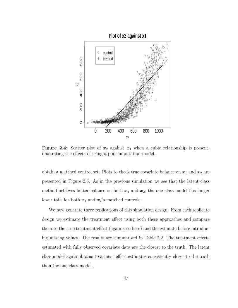
0 200 400 600 800 1000
02
00
40
06
00
80
0
Plot of x2 against x1
x1
x2
controltreated
Figure 2.4: Scatter plot of x2 against x1 when a cubic relationship is present,illustrating the effects of using a poor imputation model.
obtain a matched control set. Plots to check true covariate balance on x1 and x2 are
presented in Figure 2.5. As in the previous simulation we see that the latent class
method achieves better balance on both x1 and x2; the one class model has longer
lower tails for both x1 and x2’s matched controls.
We now generate three replications of this simulation design. From each replicate
design we estimate the treatment effect using both these approaches and compare
them to the true treatment effect (again zero here) and the estimate before introduc-
ing missing values. The results are summarized in Table 2.2. The treatment effects
estimated with fully observed covariate data are the closest to the truth. The latent
class model again obtains treatment effect estimates consistently closer to the truth
than the one class model.
37

treated latent one class
60
08
00
10
00
Balance on x1
treat latent one class
20
04
00
60
08
00
10
00
Balance on x2
Figure 2.5: Boxplots checking balance on covariates x1 and x2 respectively in thesimulation design where a cubic relationship between x1 and x2 is present.
Table 2.2: Treatment effect estimates from the fully observed data, latent class andone class models in the simulation design where a cubic relationships between thecovariates is present. The true treatment effect equals zero and the SE(YT ) ≈ 22
Estimate Rep 1 Rep 2 Rep 3Observed 30.6 42.7 22.8
Latent class 43.0 52.6 34.8One class 52.4 62.7 54.6
Linear relationship
We now consider a simulation where x1 and x2 share a linear relationship,
x1i = 50 + 0.8i+ ǫ1i, ǫ1i ∼ N(0, 75) (2.36)
x2i = 50 + 0.8i+ ǫ2i, ǫ2i ∼ N(0, 10) (2.37)
for i = 1, . . . , n. A covariate plot is given in Figure 2.6.
In this situation the one class model is a suitable model for the data and will
38
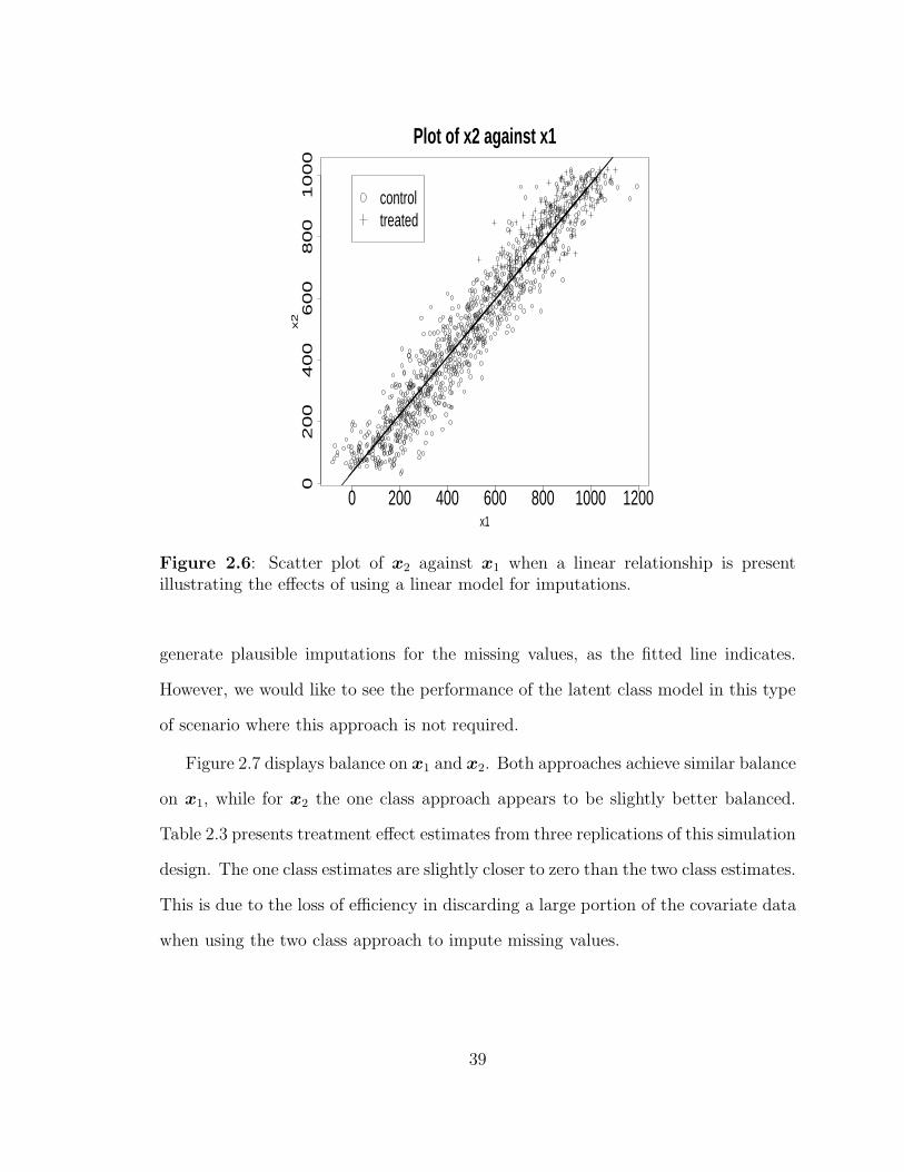
0 200 400 600 800 1000 1200
02
00
40
06
00
80
01
00
0
Plot of x2 against x1
x1
x2
controltreated
Figure 2.6: Scatter plot of x2 against x1 when a linear relationship is presentillustrating the effects of using a linear model for imputations.
generate plausible imputations for the missing values, as the fitted line indicates.
However, we would like to see the performance of the latent class model in this type
of scenario where this approach is not required.
Figure 2.7 displays balance on x1 and x2. Both approaches achieve similar balance
on x1, while for x2 the one class approach appears to be slightly better balanced.
Table 2.3 presents treatment effect estimates from three replications of this simulation
design. The one class estimates are slightly closer to zero than the two class estimates.
This is due to the loss of efficiency in discarding a large portion of the covariate data
when using the two class approach to impute missing values.
39

treated latent one class
60
08
00
10
00
Balance on x1
treat latent one class
60
07
00
80
09
00
10
00
Balance on x2
Figure 2.7: Boxplots checking balance on covariates x1 and x2 respectively in thesimulation design where a linear relationship between x1 and x2 is present.
Table 2.3: Treatment effect estimates from the fully observed data, latent class andone class models in the simulation design where a linear relationship between thecovariates is present. The true treatment effect equals zero and the SE(YT ) ≈ 14
Estimate Rep 1 Rep 2 Rep 3Observed 14.4 18.8 39.9
Latent class 18.5 25.5 45.9One class 16.5 22.8 44.9
2.4.2 Categorical and continuous covariates
We now consider a simulation involving an additional categorical covariate v1 with
three levels (indexed by 1, 2 and 3 respectively). To be consistent with Section 2.3.1,
rename the two continuous covariates x1, x2 as w1 and w2 respectively.
Covariates w1 and w2 are simulated as in Section 2.2.2 so that they have a non-
40

linear relationship. We assign levels of v1 to each unit i in the following way,
v1i = 1I(i ≤ 100) + 2I(i > 100, i ≤ 200) + 3I(i > 201, i ≤ 1000) +
2I(i > 1000, i ≤ 1100) + 1I(i > 1101, i <= 1200) (2.38)
for i = 1, . . . , n. The treatment variable is simulated as in (2.12) to have larger values
of w1 and w2. We now simulate the response y by,
yi = xi1 + x2i + 20I(w1i = 1) + 50I(w1i = 2) + 80I(w1i = 3) + ǫi, ǫi ∼ N(0, 1)(2.39)
so that there is no treatment effect. A plot of the covariates is presented in Figure 2.8
where the different symbols now correspond to different levels of v1. In this situation,
modeling continuous covariates as normal within each level of v1 may still not be a
reasonable assumption. From Figure 2.8, the continuous covariates for which v1 = 3,
(w1i, w2i), i : v1i = 3 still have a distinct non-linear relationship. Also, proportions
of each level of v1 differ for units lying in the treated space as compared to the rest
of the controls. Thus, a latent class approach in this situation may generate more
plausible imputations and result in a better balanced matched control set.
I apply both the latent class and one class models to impute missing covariates
and estimate the treatment effect. The MCMC is run for 100000 iterations with
a burn-in of 5000 iterations. True covariate balance on w1 and w2 is presented in
Figure 2.9. We see that balance on w1 is similar for both approaches, but balance
on the partially observed w2 is better when using the latent class model. Table 2.4
displays the proportion of units in each level of v1 for treated and matched controls
in both approaches. There are small gains in balancing v1 when using the latent class
approach.
41

0 200 400 600 800 1000
02
00
40
06
00
80
0
w1
w2
v1 = 1v1 = 2v1 = 3
Figure 2.8: Scatter plot of w1 and w2 indexed by the levels of v1 in the simulationwith both categorical and continuous covariates.
We now obtain treatment effect estimates from three replications of this simulation
design. Results are presented in Table 2.5. We see that the estimates obtained from
the latent class model are all closer to the truth than the estimates from the one class
model.
2.5 Breast feeding study
We now apply the latent class model to impute missing covariates in a genuine data
set. The study assesses the effect of breast feeding on child’s cognitive development
using variables from the National Longitudinal Survey of Youth (NLSY).
42
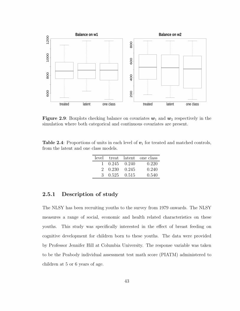
treated latent one class
60
08
00
10
00
12
00
Balance on w1
treated latent one class
20
04
00
60
08
00
Balance on w2
Figure 2.9: Boxplots checking balance on covariates w1 and w2 respectively in thesimulation where both categorical and continuous covariates are present.
Table 2.4: Proportions of units in each level of v1 for treated and matched controls,from the latent and one class models.
level treat latent one class1 0.245 0.240 0.2202 0.230 0.245 0.2403 0.525 0.515 0.540
2.5.1 Description of study
The NLSY has been recruiting youths to the survey from 1979 onwards. The NLSY
measures a range of social, economic and health related characteristics on these
youths. This study was specifically interested in the effect of breast feeding on
cognitive development for children born to these youths. The data were provided
by Professor Jennifer Hill at Columbia University. The response variable was taken
to be the Peabody individual assessment test math score (PIATM) administered to
children at 5 or 6 years of age.
43

Table 2.5: Treatment effect estimates from the fully observed data, latent classand one class models in the simulation design where both categorical and continuouscovariates are present. The true treatment effect equals zero and the SE(YT ) ≈ 19
Estimate Rep 1 Rep 2 Rep 3Observed 3.7 15.3 15.5
Latent class 26.3 36.9 38.2One class 45.4 56.3 59.9
Breast feeding duration in weeks is measured for each child, which is used to form
the treatment variable. We define a child to be treated if he or she was breastfed for
24 weeks or more. This corresponds to the advice given by the American Academy
of Pediatrics (AAP, 2005) and the WHO standard. There are other ways to define
the treatment variable, and the analysis could be repeated with different cut points
on the breast feeding duration variable. For example a unit could be defined to be
treated if breastfeed for 3 months or more, or treated units could be those that are
breastfed at all.
Fourteen background covariates are measured. Five categorical variables are in-
cluded in the analysis: the child’s race (Hispanic, black or other), the mother’s race
(Hispanic, black, asian, white, hawaiian/PI/American Indian, or other), child’s sex,
and two variables indicating whether the spouse or grandparents were present at
birth. In addition, two continuous variables were categorized. A variable measuring
weeks preterm has a large spike at zero weeks as seen in its histogram displayed in
Figure 2.10. This preterm variable was categorized into three levels; not preterm
(zero weeks), moderately preterm (one to four weeks), and very preterm (five or
more weeks), with cut points determined from guidelines in the March of Dimes
study (www.marchofdimes.com). Also, a variable which measures number of weeks
worked in the year prior to giving birth has a distinct U shape as its histogram dis-
44

plays in Figure 2.11. This variable was categorized into four levels (not worked at all,
worked between 1 and 47 weeks, worked 48-51 weeks, and worked all 52 weeks). We
also measure seven continuous variables, including difference between mother’s age
at birth and in 1979, mother’s intelligence, mother’s education, child’s birth weight,
weeks child spent in hospital, weeks mother spent in hospital, and family income.
Transformations were applied to certain continuous variables as suggested by the
Box-Cox procedure (Box and Cox, 1964), for more details refer to Appendix A.
weeks preterm
Fre
qu
en
cy
0 5 10 15
05
00
10
00
15
00
Figure 2.10: Histogram of weeks preterm for subjects in the breast feeding study
In this study, with the treatment variable as defined above, there are several
clearly imbalanced covariates. To illustrate, we focus on mother’s intelligence, mother’s
years of education, and child’s race. Box plots of observed mother’s intelligence and
education for treated and control units are presented in Figure 2.12. Table 2.6 dis-
plays the proportion of treated and control units in each level of child’s race. We
45

weeks worked before birth
Fre
qu
en
cy
0 10 20 30 40 50
01
00
30
05
00
Figure 2.11: Histogram of weeks mother worked in the year before giving birth forsubjects in the breast feeding study
can clearly see the imbalance in these variables. Treated units tend to have higher
mother’s intelligence scores, more mother’s years of education and lower proportions
of Hispanics and blacks.
Table 2.6: Distribution of child’s racerace treated control
Hispanic 0.1378 0.1903black 0.1108 0.2844other 0.7514 0.5253
There were numerous post treatment variables which are not used in estimating
the treatment effect. For example, we do not include child care arrangements or
weeks worked by the mother in the years after pregnancy. These variables may be
46

treated control
24
68
10
treated control
05
10
15
20
Figure 2.12: Box plots of mother’s intelligence score and mother’s years of educationrespectively for treated and control units before matching
affected by the treatment, hence we do not wish to treat them as covariates. We
also include only first born children in the analysis to avoid complications due to
birth order and family nesting. In addition, we discard 506 units with missing values
in their treatment variable (breast feeding duration) and 4977 units with a missing
outcome variable (PIATM). With the resulting data set, we have 2388 units with 370
treated units. Of these units there are 1306 complete cases, of which 216 are treated
units.
2.5.2 Complete Case simulation
I first evaluate the performance of the latent and one class models in achieving true
covariate balance in a simulation involving the 1306 complete cases.
I introduce missing values using the frequencies of missing data patterns present
in the original data set. This resulted in 717 units with fully observed covariates.
I then run the latent and one class models to impute the missing covariates. The
47

cell probabilities are modeled using a log linear model with main effects for each
categorical variable. The within cell means of the continuous data are modeled using
a linear model with main effects of the categorical variables. The MCMC in both
cases is run for 200000 iterations after discarding an initial 5000 as burn-in. For each
approach, I average the estimated propensity scores to select matched control sets.
Box plots of mother’s intelligence and years of education for the treated and
matched control units from both approaches are presented in Figures 2.13 and 2.14.
We see that in both approaches the imbalance has been greatly reduced for these
covariates after matching. More detailed examination of balance on these covariates is
presented in Tables 2.7 and 2.8, which presents the fifth percentiles of these covariates
for treated and matched control units. We see that for mother’s intelligence, there
is some evidence to suggest that the latent class approach achieves better balance in
the tails of the distribution, while the one class model achieves better balance in the
center. For mother’s education both approaches achieve similar balance with the one
class model doing slightly better.
We also compare proportions of child’s race for treated and control units before
and after matching in Table 2.9. We also see here that imbalance is greatly reduced
using both approaches. Thus, there does not seem to be much gain in using the latent
class model in this situation. Partly this could be due to the careful modeling of the
data prior to applying the methods, which makes normality reasonable. Additionally,
approximately 85% of units are imputed to lie in the latent class for the treated units,
so that there is not much difference in the two methods. However, the latent class
model does obtain a matched control set with characteristics similar to the treated
group, and thus we are not losing substantially when using this method.
48

treated all controls latent one class
24
68
10
Figure 2.13: True covariate balance on mother’s intelligence score in the simulationinvolving the complete cases.
2.5.3 Application to the full data
We now apply the latent class model on the original data set of 2388 units. Similar
restrictions are imposed on the cell probabilities and within cell means as in the
simulation involving the complete cases. We run the MCMC for 200000 iterations
with an additional burn-in of 5000 iterations.
We obtain the matched control set from the averaged estimated propensity scores.
The treatment effect is then computed using YT − YMC. This results in a treatment
effect estimate of −0.059 and a two-sample, pooled SE of 0.941. For alternative
approaches to estimating standard errors from propensity score matching, see Hill
and Reiter (2006). For the full sample YT − YC = 5.23 (SE 0.741). We are thus
significantly closer to zero when applying this approach to estimate the treatment
49

treated all controls latent one class
05
10
15
20
Figure 2.14: True covariate balance on mother’s years of education in the simulationinvolving the complete cases.
effect. Similar data were analyzed by Der et al. (2006), who took a model based
approach to infer about the treatment effect. They also found that the effect of
breast feeding was minimal.
We also consider using the one class model to impute missing values and estimate
the treatment effect. The treatment effect here is estimated to be 0.959 (SE 0.961).
Thus there is approximately a one point difference in the treatment effect estimates
using these approaches, which is not of much practical significance. Approximately
85% of units are imputed to be in the latent class for the treated units, and so gains
from using this model are small. It should be noted, though, that certain outlying
controls, for example a unit with many weeks spent in the hospital, are never in the
latent class for treated units. Thus, the latent class does not allow this outlying unit
50

Table 2.7: 5th percentiles of mother’s intelligence for treated and matched controlsfrom the latent and one class models
percentile treat latent one class5 2.83 3.16 3.16
10 4.00 4.18 4.3015 4.82 4.92 5.0020 5.66 5.48 5.5725 6.48 5.92 5.9230 6.78 6.44 6.6035 7.21 6.84 7.0740 7.42 7.55 7.3545 7.62 7.92 7.6550 7.87 8.06 7.9455 8.19 8.19 8.1960 8.43 8.37 8.3765 8.60 8.59 8.5470 8.83 8.77 8.7275 8.94 8.94 8.8980 9.22 9.17 9.0685 9.43 9.26 9.2290 9.62 9.46 9.4695 9.80 9.75 9.75
to influence the imputation model. This highlights an advantage of the approach:
in data with controls in a distant region of the space, it can reduce the impact on
imputations for units in the region of plausible matches.
2.6 A simpler alternative
We now switch focus to an alternative idea for imputing missing covariates in obser-
vational studies. The goal is the same: de-sensitize imputations of missing covariates
in the matched region to the effect of outlying controls. However, this approach
involves less computations in finding the matched set. It is also compatible with
standard imputation software and thus reduces the burden on the analyzer.
51

Table 2.8: 5th percentiles of mother’s education in years for treated and matchedcontrols from the latent and one class models
percentile treat latent oneclass5 10 11 10
10 12 12 1215 12 12 1220 12 12 1225 12 12 1230 12 12 1235 12 12.25 1240 13 13 1345 14 14 1450 14 14 1455 15 14 1460 15 15 1565 16 15.75 1670 16 16 1675 16 16 1680 16 16 1685 16 16 1690 17 17 1795 18 18 18
I first describe the method, which I call winnowing. I then evaluate this approach
in a simulation study. Finally, I apply this method to the breast feeding study
discussed above.
2.6.1 Winnow method
The winnow method finds a matched control set by gradually reducing the set of
possible matched controls. The algorithm is described below.
1. First, multiply impute the missing values m times using standard MI software
and estimate the propensity scores.
2. Next, find the k-closest controls for each treated unit using a without replace-
52

Table 2.9: Distribution of true child’s race for treated and matched controls usinglatent and one class models
race treated all controls latent one classHispanic 0.1528 0.1844 0.1296 0.1667
black 0.0926 0.2697 0.1111 0.0833other 0.7546 0.5459 0.7593 0.7500
ment pair matching scheme. This results in a reduced data set comprising
(k + 1)nT units.
3. Re-impute missing values in this new data set again using standard MI software
and now find the k − 1-closest controls.
4. Continue this process until k = 1 and a matched control set is obtained.
This approach thus first discards a set of controls unlikely to be selected as matches.
It then gradually reduces the set of remaining controls until a matched control set is
obtained. We can compare this method to an approach that skips steps 2-4 and finds
the matched control set after the first round of multiple imputation, we call this the
once only approach.
2.6.2 Simulation result
We illustrate the winnow approach with the simulation design in Section 2.2.2 and
described in Figure 2.1. I apply the winnowing method to this design with k =
3 initially, and consider the true covariate balance and treatment effect estimate.
Figures 2.15 and 2.16 summarize the true covariate balance on x1 and x2, respectively,
for both the winnow and once only approaches. The once only approach tends to
have longer lower tails in the distribution of its matched controls, particularly for x1.
The winnow method thus results in a better balanced matched control set.
53

treated winnow once only
50
07
00
90
01
10
0
Figure 2.15: Boxplots of x1 for treated units and matched controls from the winnowand once only approaches
I now replicate the simulation design 500 times, each time estimating the treat-
ment effect from the winnow and once only approaches. I also consider the treatment
effect estimated with fully observed covariates in each replication. The results are
summarized in Figure 2.17. We see that the treatment effect estimates based on fully
observed covariates tends to be closest to the truth as expected. The winnow ap-
proach tends to get closer to the truth compared to the once only and thus performs
better in this situation.
2.6.3 Breast feeding study results
I now apply the winnow method to the breast feeding study discussed before. To
multiply impute the data, the MICE (Multiple Imputation Via Chained Equations)
54
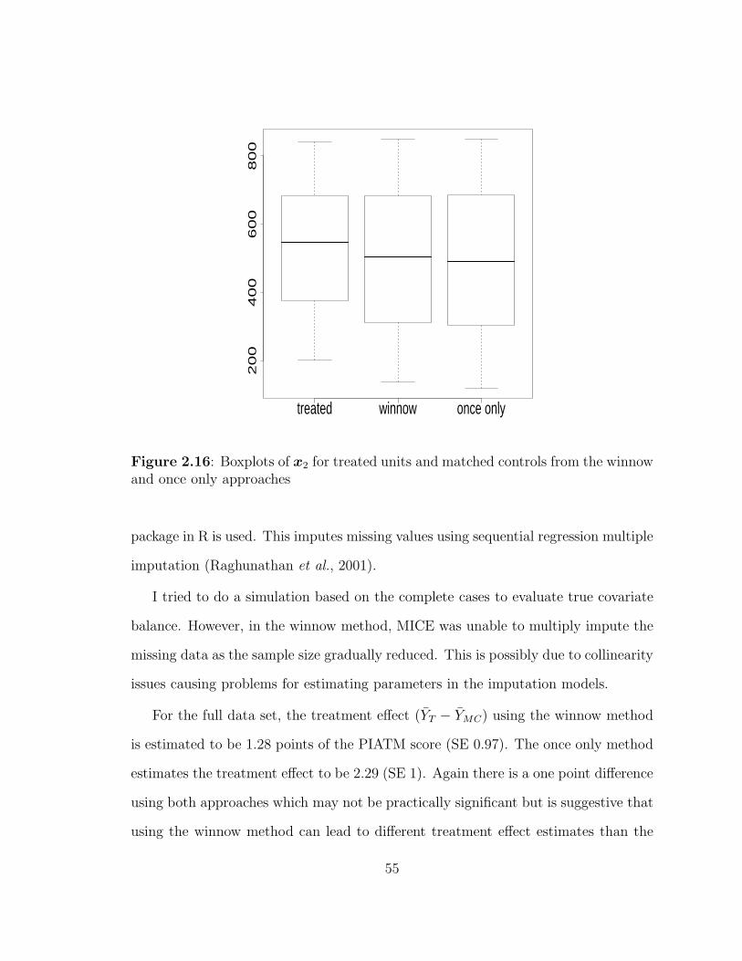
treated winnow once only
20
04
00
60
08
00
Figure 2.16: Boxplots of x2 for treated units and matched controls from the winnowand once only approaches
package in R is used. This imputes missing values using sequential regression multiple
imputation (Raghunathan et al., 2001).
I tried to do a simulation based on the complete cases to evaluate true covariate
balance. However, in the winnow method, MICE was unable to multiply impute the
missing data as the sample size gradually reduced. This is possibly due to collinearity
issues causing problems for estimating parameters in the imputation models.
For the full data set, the treatment effect (YT − YMC) using the winnow method
is estimated to be 1.28 points of the PIATM score (SE 0.97). The once only method
estimates the treatment effect to be 2.29 (SE 1). Again there is a one point difference
using both approaches which may not be practically significant but is suggestive that
using the winnow method can lead to different treatment effect estimates than the
55

observed winnow once only
−2
00
20
40
60
80
Figure 2.17: Treatment effect estimates over repeated simulations. The dotted lineindicates the true treatment effect of 0.
once only approach.
2.7 Discussion
Propensity score matching is an appealing approach to estimate treatment effects
in observational studies. However, when missing data are present, problems can
arise when using multiple imputation techniques. Matching based on implausible
imputations can affect the true covariate balance and thus affect the estimate of the
treatment effect.
I proposed a latent class model to address this issue. Simulation studies show
the potential for gains over standard multiple imputation approaches, without huge
56

sacrifice in accuracy when a one class model is appropriate. I applied this approach
to a breast feeding study using data from the NLSY. A simulation using the com-
plete cases shows the covariate imbalance is significantly reduced using this method
compared to the full data, although it is not much different than the one class ap-
proach. This is because approximately 85% of units are grouped into the latent class
for treated units, suggesting the one class model is a reasonable model for the data.
This is one case where the latent class model did not hurt, as in the third simulation
in Section 2.4.1 where a linear relationship is present between the covariates. This is
consistent with my conjecture that the latent class approach can limit the impact of
bad imputation models while not losing too much when the approach is not required.
In future research, I would like to extend the approach to include multiple latent
classes. This may generate more plausible imputations than the two class approach.
A natural question then arises about the optimal number of latent classes. An inter-
esting approach would be to use Dirichlet Process models to induce covariate clusters
on which an imputation model can be based. Another possible extension includes
addressing the issue of missing values in the response variable using this approach.
57

Chapter 3
Estimating treatment effects withmultiply imputed propensity scores
In the previous chapter, I proposed a latent class model to multiply impute missing
covariates in observational studies. From each multiply imputed data set, the ana-
lyst can estimate propensity scores. With these, the analyst has several options for
estimating treatment effects. I consider two such approaches here. The first is to
average the estimated propensity scores across the imputed data sets. The analyst
uses these to estimate the treatment effect with matching techniques. This was the
method used in Chapter 2. We call this approach the Across method. The second
is to estimate the treatment effect within each imputed data set by matching on the
corresponding estimated propensity scores. The analyst averages the treatment effect
estimates from the imputations to obtain a point estimate of the treatment effect.
We call this approach the Within method. These approaches are also described in a
technical report by Hill (2004).
Both these approaches may be reasonable ways to estimate treatment effects
with missing data; however, they can give different results, even when the imputation
model is appropriate for the missing values. For example, in the analysis of the breast
feeding study in Section 2.5, the Across method without a latent class imputation
model estimated a treatment effect of 0.96, whereas the corresponding Within method
estimated a treatment effect of 1.14. While small, this difference suggests that the
Across and Within methods could have different properties.
There are several factors influencing how the treatment effect is computed in the
Across and Within approaches. The model used to impute the missing values can
58

clearly affect the treatment effect estimate, as shown in Chapter 2. The model to
estimate the propensity scores may depend on imputed values. This in turn affects
which records are selected in the matched control set. In addition, the nature of
the response surface influences the estimate of treatment effects. In this chapter, I
investigate the behavior of the Across and Within approaches to estimate treatment
effects, with the goal of making inroads into differentiating their properties. This is
a challenging problem and is not fully resolved here. The purpose of this chapter is
to layout the problem and present some initial findings.
Section 3.1 formalizes the Across and Within approaches. Section 3.2 illustrates
the behavior of the Across and Within approaches in two simulation studies. Section
3.3 investigates the variance of the treatment effect estimator from both methods
from a randomization based perspective, focusing on a particular component of this
variance. Section 3.4 examines how this variance component depends on the num-
ber of imputations. Section 3.5 proposes some techniques to estimate this variance
component. Section 3.6 presents simulation studies to investigate the properties of
multiple imputation combining rules for this setting. Finally, Section 3.7 concludes
the chapter.
3.1 Across and Within approaches
We first define the notation used to frame the problem. For an explanation of the
treatment effect being studied and propensity score matching techniques applied, see
Chapter 2 of this thesis. As in Section 1.1, define an n × p matrix of covariates
X = (x1, . . . ,xn)′, where xi = (xi1, . . . , xip)
′ corresponds to the ith unit’s covariates,
for i = 1, . . . , n. For each xi, define a vector of corresponding missing data indicators
mi = (mi1, . . . , mip)′, where mij = 1 indicates xij is missing, and mij = 0 indicates
59

xij is observed, for j = 1, . . . , p. Let M = (m1, . . . ,mn)′ be the n × p matrix of
missing data indicators for X. Also define Xmis = xij : (i, j) : mij = 1 and
Xobs = xij : (i, j) : mij = 0 to represent the missing and observed parts of X.
In multiple imputation, values of Xmis are filled in m times with draws from the
posterior predictive distribution, p(Xmis|Xobs), resulting in m completed data sets
X(1)com, . . . ,X
(m)com. For each X
(k)com, let e(x
(k)i,com) be the estimated propensity score for
unit i, where i = 1, . . . , n and k = 1, . . . , m.
The Across approach estimates the propensity score for each unit by averaging
over the imputations. For each unit i, estimate its propensity score with
eA,m(xi) =
∑mk=1 e(x
(k)i,com)
m. (3.1)
Call the set of all units’ propensity scores eA,m = (eA,m(x1), . . . , eA,m(xn))
′. Analysts
use these to find a matched control set and compute Y A,mmc , the average of the control
units’ outcomes in this matched set. From m imputations of the missing data, one
estimates the treatment effect in the Across approach with
τA,m = YT − Y A,mmc , (3.2)
which compares the mean of all observed treated units’ outcomes in the study with
the mean of matched control units’ outcomes selected in the Across approach.
The Within approach uses the propensity scores estimated from each imputed
data set, e(X(k)com) = (e(x
(k)1,com), . . . e(x
(k)n,com))′, to obtain a matched control set in
each data set. Let, Y(k)mc be the average of the outcomes for the matched controls
in data set k, where k = 1, . . . , m. Let Y W,mmc =
Pmk=1 Y
(k)mc
m. The treatment effect is
60

estimated in the Within approach with
τW,m = YT − Y W,mmc . (3.3)
That is, the treatment effect is estimated by comparing the mean of all the treated
units’ outcomes in the study to the mean of the m sets of matched control units’
outcomes.
3.2 Illustrating differences between the two ap-
proaches
I now illustrate the differences between these approaches with two simulations. I first
generate a covariate data set X with n = 240 records such that
xi ∼ N(µ,Σ), (3.4)
with µ = (10, 10)′, and Σ =
5 2.5
2.5 5
. I generate response Yi with
Yi = xi1 + xi2 + ǫi, ǫi ∼ N(0, 1) (3.5)
for i = 1, . . . , 240, so that there is no treatment effect. The two simulations differ in
how I assign treatment.
61

3.2.1 Simulation 1 - treatment assignment depends on x1
To assign treatment in this first simulation, I first order the rows of X in increasing
order of x1. Units are allocated to treatment according to,
p(Ti = 1) = 0.25I(i > 160), (3.6)
where I(.) is an indicator variable taking 1 on the set of units i defined in (.) and
0 for all other i. There are 20 treated units and 220 control units. A covariate
plot summarizing this set up is given in Figure 3.1. With this set up, treatment
assignment is dependent only on x1. Missing values are introduced in x2 with an
MCAR mechanism so that approximately 35% of units’ values of x2 are missing. I
impute missing values from a normal linear regression, which is their true posterior
predictive distribution.
0 5 10 15
24
68
10
12
14
16
Plot of x2 against x1
x1
x2
controltreated
Figure 3.1: Plot of the covariate distribution in the simulation design where treat-ment assignment depends on x1
62

I repeatedly generate this simulation design 1000 times. Each time I estimate
treatment effects in the Across and Within approaches. This corresponds to evaluat-
ing the performance of the two approaches over different realizations of an observed
data set from the population. Table 3.1 summarizes the results. Both the Across
and Within approaches have similar estimates of the treatment effect, which are also
close to the true treatment effect estimate of zero. However, the Across approaches
tend to have higher variances than the Within approaches. The Within variances
appear to decrease as m increases, but the trend appears to be non-linear in the
Across variances.
Table 3.1: Treatment effect estimates from the Across and Within approaches inthe simulation design where treatment assignment depends on x1
m Across estimate Across variance Within estimate Within variance5 −0.0130 0.2962 0.0230 0.193810 −0.0327 0.3216 0.0245 0.177715 −0.0218 0.3223 0.0206 0.176520 −0.0216 0.3122 0.0218 0.173750 −0.0104 0.3040 0.0227 0.1684
In this simulation design, treatment assignment only depends on x1, which is
a fully observed variable in the sample. Propensity scores will thus be determined
using essentially x1 only, so that the missing data play a minor role here. Thus, it is
not surprising that both the Across and Within methods result in similar reductions
in bias. Nonetheless, this is a situation where the Within approaches dominate on
mean squared error, at least for these values of m.
63

3.2.2 Simulation 2 - treatment assignment depends on x2
In the second simulation, X and Y = (Y1, . . . , Y240)′ are simulated as before, but
I now order X in increasing order of x2. Treatment is then assigned as in (3.6).
Thus, treatment assignment depends only on x2. There are 20 treated units and 220
control units. A covariate plot summarizing this design is given in Figure 3.2. As
before, we make approximately 35% of x2 to be missing with an MCAR mechanism,
and we use the same model to impute missing values.
0 5 10 15
24
68
10
12
14
16
Plot of x2 against x1
x1
x2
controltreated
Figure 3.2: Plot of the covariate distribution in the simulation design where treat-ment assignment depends on x2
We again estimate the treatment effect from the Across and Within methods over
1000 replications of the simulation. Table 3.2 summarizes the results for different m.
The Within estimates have consistently larger bias than the Across estimates. The
bias in the Across estimates diminishes as m increases. The variances in the Within
approach, however, still tend to be lower than the variances in the Across approach
64

and appear to decrease with m.
Table 3.2: Treatment effect estimates from the Across and Within approaches inthe simulation design where treatment assignment depends on x2
m Across estimate Across variance Within estimate Within variance5 0.4087 0.3621 0.8456 0.211810 0.2126 0.3772 0.8418 0.168815 0.1485 0.3438 0.8354 0.155920 0.1179 0.3663 0.8363 0.150750 0.0232 0.3589 0.8405 0.1412
In this simulation design, treatment assignment depends on x2, which is a partially
observed variable. Thus, imputation of the missing values plays more of a role here
in finding the matched control set than in the simulation in Section 3.2.1. This might
explain the large differences between the treatment effect estimates in the Within and
Across methods. Because the Within approach finds matched controls within each
imputed data set, it is possible that its treatment effect estimate is more sensitive to
the imputations than the Across approach. On the other hand, the Across approach
averages propensity scores over the imputations and thus implicitly integrates out
the missing data to estimate propensity scores. Thus, the missing data may have less
of an impact in the Across approach estimates of the treatment effect, particularly
with larger values of m. This is reflected in the estimates of the Across approach
being similar in both simulations for m = 50 and close to zero.
To summarize the two sets of simulations, it is not clear which approach tends to
result in smaller biases, although the simulations suggest greater potential for bias
reduction with the Across approach. This is a topic I plan to study in more depth
in my future research. I now proceed to examine the variance of both approaches in
more detail.
65

3.3 Randomization based variance
We consider units in the study to be sampled from some finite population. The
sampling mechanism is denoted by S. From a randomization based perspective, vari-
ability in the treatment effect estimates, τA,m or τW,m, are due to different realizations
of S and M . We thus can decompose the variance of the treatment effect for τA,m
as,
V ar(τA,m) = V ar(E(τA,m|S)) + E(V ar(τA,m|S))
= V ar(E(E((τA,m|S,M))) + E(V ar(E(τA,m|S,M)))
+E(E(V ar(τA,m|S,M))). (3.7)
We can similarly decompose τW,m. It is difficult to compute the above variance
analytically. The units in the matched control set are selected in a complicated way,
and the variance needs to calculated over repeated realizations of the sampling and
missingness mechanisms.
We are, however, interested in comparing the variances from the Across and
Within approaches to estimate a treatment effect. If we assume that given a sample
of the data, and a realization of the missing pattern, the two approaches have the
same expectation, i.e.
E(τA,m|S,M) = E(τW,m|S,M), (3.8)
then the first two terms in (3.7) are the same for both the Across and Within ap-
proaches. This is a strong assumption and is not necessarily true in practice, as seen
in Section 3.2. However, this gives us a starting place for comparing the variances
for both approaches.
66

We focus on the third component of the variance in (3.7). This component involves
taking expectations over S and M , which again is hard to do analytically. We thus
condition on a particular realization of S and M and so consider
V ar(τA,m|S,M) = V ar(YT − Y A,mmc |S,M) (3.9)
and similarly for τW,m. In (3.9), YT is fixed given S. The variability comes from how
we pick the matched control set. This depends implicitly on the model to impute
the missing values and the approach used. We consider each control record i having
some probability πi to be selected as a match to any treated unit, where i = 1, . . . , nc
and nc is the number of control units in S. Motivated by the ideas of Horvitz and
Thompson (1952), the mean of the matched control records selected from either the
Across or Within approach can be expressed as,
Ymc =
∑nc
i=1 YiIinT
, (3.10)
where Ii = 1 with probability πi and Ii = 0 with probability 1 − πi.
The match probabilities πi differ for the Across and Within approaches. Denote
these as πA,mi and πW,mi , respectively. In the Within approach, control units are
repeatedly matched for each imputed data set resulting in Y(k)mc , for k = 1, . . . , m. The
match probability does not depend on the number of imputations, so that πW,mi = πWi .
67

Hence, the variance of the treatment effect estimate in the Within approach is,
V ar(τW,m|S,M) = V ar(
∑mk=1 Y
(k)mc
m|S,M)
=1
m× n2T
( nc∑
i=1
Y 2i π
Wi (1 − πWi )
+∑
i6=j
YiYj(πWij − πWi π
Wj )
), (3.11)
where πWij is the probability both units i and j are jointly matched in the Within
approach. In the Across approach, we average the propensity scores for each unit i
across m imputations of the missing data. We then find a matched control set based
on the averaged propensity scores. The match probabilities in the Across approach
thus implicitly depend on m. The variance of the Across approach is then
V ar(τA,m|S,M) = V ar(Y A,mmc |S,M)
=1
n2T
( nc∑
i=1
Y 2i π
A,mi (1 − πA,mi )
+∑
i6=j
YiYj(πA,mij − πA,mi πA,mj )
). (3.12)
3.4 Across and Within variance for different num-
ber of imputations
We now consider the effects of different numbers of imputations, m, on the variance
of treatment effects estimated for a given S and M . We wish to compare (3.11) and
(3.12).
68

When we only impute the data once, i.e. m = 1, we have
e(x(k)i,com) =
∑mk=1 e(x
(k)i,com)
m
= e(A,m)(xi) (3.13)
for i = 1, . . . , n. Hence,
τ (W,1) = τ (A,1) (3.14)
and the Across and Within approaches are equivalent. Thus, πW = πA,1 and this
implies
V ar(τA,1|S,M) = V ar(τ (W,1)|S,M). (3.15)
We also can consider this component of the variance in both approaches as m
tends to infinity. In the Within approach, from (3.11) we see that the variance
decreases at the rate of 1m
. Hence, as m goes to infinity, the variance in the Within
approach goes to zero. In the Across approach, we have only one estimate of the
treatment effect based on the average of the propensity scores over imputations of
the missing data. To investigate this variance, we first consider
V ar(eA,m(xi)) = V ar(
∑m
k=1 e(x(k)com,i)
m) (3.16)
for i = 1, . . . , n. Each e(x(k)com,i)) is bounded in [0, 1], so that
V ar(
∑m
k=1 e(x(k)com,i)
m) ≤ 1
4m. (3.17)
69

Thus, each unit’s propensity score in the Across approach stabilizes to some value as
m → ∞. For a given set of propensity scores, the matched control set is obtained
deterministically, and so in the Across approach πA,mi → 0 or 1 as m → ∞ for
i = 1, . . . , nc, unless two or more records have the same propensity scores. When t
control units’ propensity scores are tied with t ≥ 2, the analyst typically randomly
chooses a matched control from among these t units. We do not consider the issue
of ties here, since for continuous covariates ties are unlikely. When πA,mi = 0 or 1,
we have
πA,mi (1 − πA,mi ) = 0 (3.18)
πA,mij − πA,mi πA,mj = 0. (3.19)
Equation (3.18) is obvious as the only possibilities are 0 × 1 or 1 × 0. For (3.19),
first consider the situation when πA,mi = πA,mj = 0. In this case, units i and j are
never matched and thus will never be jointly matched so that πA,mij = 0. Similarly,
when πA,mi = πA,mj = 1 units i and j are always matched and hence πA,mij = 1. When
πA,mi = 1 and πA,mj = 0, unit i is always matched and unit j is never matched,
so that units i and j cannot be jointly matched and πA,mij = 0. Similarly, when
πA,mi = 0 and πA,mj = 1, πA,mij = 0. Hence, from (3.18) and (3.19), we have
V ar(Y A,mmc |S,M) → 0 as m → ∞. (3.20)
Thus for m = 1 and m = ∞, the Across and the Within approach have the same
variances conditional on S and M . However, for modest m the variances of the two
approaches may differ. This explains some of the differences in variance evident in
Tables 3.1 and 3.2
70

3.5 Estimating the variance
To estimate the variance in the Within approach for a fixed S and M , we can estimate
the match probabilities πWi for each control unit i and joint match probabilities πWij
for control units i and j. We estimate πWi with the proportion of times unit i was
selected as a match in the m imputed data sets. Similarly, we estimate πWij with the
proportion of times both units i and j are jointly matched in the m imputations.
Alternatively, we can estimate the variance in the Within approach by computing
ˆV ar(τ (W,m)|S,M) =1
m×
∑m
k=1(Y(k)mc −
Pmk=1 Y
(k)mc
m)2
m− 1
(3.21)
i.e. the sample variance of Y(k)mc divided by m.
The match probabilities in the Across approach are difficult to estimate, as we
only obtain one matched control set from the m imputations of the missing data.
One way we might directly estimate this variance is by repeatedly resampling the m
imputed data sets as follows.
• First, resamplem completed data sets with replacement from X(1)com, . . . ,X
(m)com
resulting in X(1)com, . . . , X
(m)com imputed data sets.
• Compute Y A,mmc from the m resampled data sets. Call this Y
A,m,(1)mc .
• Repeat this process Z times, each time computing YA,m,(l)mc , where l = 1, . . . , Z.
• Estimate the variance with,
V arboot(τA,m|S,M) =
∑Z
l=1(YA,m,(l)mc −
PZl=1 Y
A,m,(l)mc
Z)2
Z − 1(3.22)
Resampling is commonly used to estimate variances in complex survey designs (Lohr,
71

1999). In this way, we avoid having to estimate the match probabilities πA,mi and
πA,mij .
To check how well this resampling approach estimates (3.12), we adapt the simu-
lation design in Section 3.2.1. We generate an observed data set with missing values,
and impute the missing data m times. We estimate the variance of the treatment
effect estimate from the Across approach by computing V arboot(τA,m|S,M). We
repeat this process r = 500 times for the given S and M , each time computing
V ar(l)
boot(τA,m|S,M), where l = 1, . . . , r. We then compare the average of these esti-
mates,Pr
l=1dV ar(l)boot(bτA,m|S,M)
r, to the “true” variance of the Across approach treatment
effect estimate, which we calculate with
V ar(τA,m|S,M) =
∑r
l=1(τA,m,(l) −
Prl=1 bτA,m,(l)
r)2
r − 1, (3.23)
where τA,m,(l) is the Across estimate in the lth repetition of the multiple imputation
of the data. Table 3.3 summarizes the results of this process for three different
realizations of S and M , where m = 20, and Z = 100. The bootstrap estimate is not
always close to the true variance in the Across method. In the first replication, the
bootstrap estimate is approximately 40% higher than the true variance; otherwise, it
does reasonably well. This indicates that the performance of this estimator is sensitive
to S and M . More analysis is required to assess the validity of this estimator for
different realizations of S and M .
Another way to estimate the variance of the Across approach given S and M
is to repeatedly multiply impute the missing data and estimate the variance using
(3.23). This corresponds to generating m× r imputations in total. Some interesting
questions then arise. If we are repeating the multiple imputation process, why not
use these to estimate the treatment effect? Also, how should we allocate m and r for
72

Table 3.3: Performance of the bootstrap estimate of the variance in the Acrossapproach conditional on S and M
Rep Bootstrap estimate True variance1 0.0464 0.03292 0.0648 0.06803 0.1338 0.1331
a given number of m× r imputations of the data? We investigate this further in the
next section.
3.6 Repeatedly multiply imputing the data
When multiply imputing the missing data m times in the Across approach, we can
consider repeating this process r times. That is, we create m data sets, average
propensity scores, and match r times. We can then estimate the treatment effect
with
τA,m,r =
∑rl=1 τ
A,m,(l)
r. (3.24)
The Within approach is a special cases of (3.24) when m = 1, i.e.,
τW,r = τA,1,r. (3.25)
3.6.1 Trade off between m and r
We can investigate the possible trade offs in bias and variance for estimates of the
treatment effect for different m and r. We illustrate this using the two simulation
designs discussed in Section 3.2. In both simulation designs, we calculate τA,m,r for
73

different (m, r) combinations such that m × r = 100. We simulate 1000 different
realizations of S and M .
Tables 3.4 and 3.5 present the results of the treatment effect estimates in the
simulation designs from Sections 3.2.1 and 3.2.2, respectively. In Table 3.4, we see
that the effect of increasing m on reducing bias is not that great. This is because
the bias is already small with m = 1. This reflects what was seen in Table 3.1. As
r increases, there is a reduction in the variance of the estimator. This is because
we are averaging treatment effects over r repetitions. As bias is small, the variance
component dominates the mean squared error, with m = 1 and r = 100 having the
smallest mean squared error.
Table 3.4: Treatment effect estimates for different allocations of m and r in thesimulation design where treatment assignment depends on x1
m r estimate variance MSE1 100 0.0241 0.1673 0.16792 50 0.0056 0.1779 0.17795 20 −0.0091 0.1967 0.1968
10 10 −0.0122 0.2103 0.210420 5 −0.0137 0.2264 0.226650 2 −0.0138 0.2521 0.2523
100 1 −0.0119 0.2964 0.2965
In Table 3.5, we again see that the variance tends to decrease as r increases. In
this simulation design, increasing m reduces the bias. This effect is also evident in
Table 3.2. There is thus a bias and variance trade off for different allocations of m
and r in this simulation design. The optimal allocation given m× r = 100 could be
when m = 10 and r = 10, as this has the smallest the mean squared error in this
simulation. For different values of m × r there may be different profiles in the bias
and variance trade off. For example, for very large m, by (3.20) r is irrelevant because
74

τA,m,(l) is fixed for any l. Figuring out the value of m such that V ar(Y A,mmc |S,M) = 0
is an open area of research.
Table 3.5: Treatment effect estimates for different allocations of m and r in thesimulation design where treatment assignment depends on x2
m r estimate variance MSE1 100 0.8376 0.1390 0.84062 50 0.6687 0.1368 0.58415 20 0.3989 0.1498 0.3089
10 10 0.2170 0.1771 0.224220 5 0.1106 0.2194 0.231650 2 0.0252 0.2870 0.2876
100 1 −0.0139 0.3829 0.3831
3.6.2 Multiple imputation variance combining rules
We now turn our attention to applying the standard multiple imputation combining
rules from m × r imputations of the missing data to estimate the variance of the
treatment effects.
To estimate the variance of τA,m,r, we need estimates of the within and between
imputation variability, U and B respectively. To estimate U , we need associated
measures of uncertainty for each τA,m,(l) which we call u(l), where l = 1, . . . , r. The
quantity U is then estimated byPr
l=1 u(l)
r. We estimate B by (3.23). We can then
combine U and B as described in (1.14) to estimate V ar(τA,m,r).
Determining an appropriate estimate u(l), is complicated since computing each
τA,m,(l) involves matching. Instead, we focus on how well the multiple imputation
combining rules estimate V ar(τA,m,r|S) in the simulation designs. According to mul-
tiple imputation theory, B(1 + 1r) is supposed to estimate V ar(τA,m,r|S). To ver-
ify whether this estimate is reasonable, for a given sample we repeatedly generate
75

patterns of missing values 1000 times. Each time we estimate the between imputa-
tion variance, B(j), using (3.23) and compute the treatment effect estimate τA,m,r,(j),
where j = 1, . . . , 1000. We then compareP1000
j=1 B(j)(1+ 1r)
1000to the true variance, which
we calculate with,
V ar(τA,m,r|S) =
∑1000j=1 (τA,m,r,(j) −
P1000j=1 bτA,m,r,(j)
1000)2
999. (3.26)
Tables (3.6) and (3.7) summarize the results from the simulation designs in Sections
3.2.1 and 3.2.2 respectively. We see that in both tables B(1 + 1r) is far too large
relative to the true variance.
Table 3.6: Evaluating estimate of B in the simulation design where treatment as-signment depends on x1
m r B(1 + 1r) True variance
5 20 0.0796 0.025710 10 0.0727 0.037020 5 0.0245 0.0105
Table 3.7: Evaluating estimate of B in the simulation design where treatment as-signment depends on x2
m r B(1 + 1r) True variance
5 20 0.1781 0.037110 10 0.1524 0.048220 5 0.0628 0.0422
Apparently, the standard multiple imputation combining rules to infer about the
treatment effect cannot be justified here. It appears that new multiple imputation
combining rules need to be derived in this setting. I plan to look into new combining
rules as part of my future research.
76

3.7 Concluding remarks
In this chapter, I laid out the problem of estimating treatment effects when there are
missing covariates, using two approaches. There is evidence that the two approaches
have different properties, both in their point estimates and variances. For a fixed
m × r neither the standard Across approach, when r = 1, nor the standard Within
approach, when m = 1 may be optimal. The simulation results in Table 3.5 show
the mean squared error is smallest when m = r = 10.
The simulations generated some speculative hypotheses that I would like to in-
vestigate in future research.
1. The Across approach has the potential for greater bias reduction than the
Within approach. This was seen in Section 3.2.
2. When treatment assignment does not depend strongly on missing values, both
approaches will reduce bias similarly.
3. For modest m × r the standard Within approach (m = 1) estimates of the
treatment effect have a smaller variance than the standard Across approach
estimates (r = 1).
I plan to investigate these hypotheses more thoroughly in future research. Other
areas include the following. I would like to obtain expressions for the variance. This
is challenging, but it may be possible to find conditions when the mean squared error
of one approach exceeds the other. I would like to develop a Bayesian approach to
this problem, if one exists. I would like to find new multiple imputation combining
rules, since standard ones are inadequate in this setting, even just to estimate the
between imputation variability.
77

Chapter 4
Two Level Stochastic Search VariableSelection in GLMs with MissingPredictors
4.1 Introduction
In regression, one issue that is routinely encountered is how to select a subset of the
available predictors that are important in explaining the response. In many fields,
this variable selection problem is faced in essentially every study that is conducted.
For example, in epidemiologic studies of exposure-disease relationships, investiga-
tors typically collect information on multiple potential risk factors and confounding
variables. Clearly, problems can be encountered if all these variables are included as
predictors, so epidemiologists tend to discard covariates that do not have a significant
impact on disease risk, unless these covariates are the primary exposures of interest
or there is strong prior knowledge that they should be included.
Stepwise selection is the most widely-used automated algorithm for selecting vari-
ables to include in a regression model, with many variants possible depending on the
starting model, the manner in which variables are added or deleted, and the criteria
for deciding whether a predictor significantly improves goodness-of-fit. For example,
forward selection sequentially adds predictors, keeping those that improve the AIC,
BIC, or have p-values in a likelihood ratio, Wald or score test below some pre-specified
threshold. For generalized linear models (GLMs), the order in which variables are
added and the criteria used can have a substantial impact on the final subset of vari-
ables that are selected. In addition, basing inferences on the model selected from a
78

stepwise procedure without accounting for uncertainty in the selection process can
lead to highly misleading results. For example, there will be a greatly inflated type
I error rate and the parameter estimates will be biased away from zero, particularly
if there are many candidate predictors.
A number of strategies have been proposed to address such problems, with the
focus in this chapter on Bayesian model averaging approaches allowing for missing
predictors. In the Bayesian paradigm, one can assign posterior probabilities to each
of the models in a list of a priori plausible models. To avoid uncertainty in model
selection, one can then average over models in the list using posterior probability
weights in performing inferences and predictions. In terms of prediction, Bayesian
model averaging has been shown to have better performance compared with using
any single model (Raftery et al., 1997). For a review of Bayesian model averaging
see Hoeting et al. (1999) and Clyde and George (2004).
In variable selection problems, the list of models under consideration corresponds
to the 2p possible subsets of a set of p candidate predictors. Clearly, the number
of models rapidly becomes enormous as p increases, so there is a need for efficient
methods for searching for high posterior probability models, while also estimating
posterior model probabilities and the posterior distributions for the coefficients in
each model. A widely used strategy for addressing this problem is to embed all
the models in a full model containing all the predictors, and then allow predictors
to drop out by choosing a mixture prior for the coefficients with one component
concentrated at zero (Mitchell and Beauchamp, 1988). One can then use a Gibbs
sampling algorithm for simultaneous model search and posterior computation, with
such an approach referred to as stochastic search variable selection (SSVS) (George
and McCulloch, 1993, 1997).
When missing values are present in the covariates SSVS algorithms cannot be
79

applied directly. One commonly used strategy is to discard subjects with any miss-
ing predictors (complete case analysis), but this can be a sizeable proportion of the
subjects in variable selection contexts, as one would need to discard subjects with
missing values in any of the candidate predictors. Further, when missing patterns are
not MCAR this approach can lead to biased inferences. Bayesian models can easily
accommodate missing predictors by placing a joint model on the distribution of the
predictors and then imputing the missing values within an MCMC algorithm. In
the variable selection setting, with the response and predictors following a multivari-
ate normal distribution, such an approach was implemented by Yang et al. (2006).
This article addresses a much broader class of models involving mixed categorical
and continuous variables, while also allowing model selection for the predictor com-
ponent. For related work see Madigan and York (1995) and York et al. (1995) who
accommodate missing data when model averaging with Bayesian graphical models.
Outside of the variable and model selection context, a standard approach for
specifying the joint distribution of the predictors, while allowing these predictors
to have different measurement scales, is to choose a sequence of GLMs (see, for
example, Lipsitz and Ibrahim (1996); Ibrahim et al. (1999)). However, following
such an approach one faces uncertainty in how to specify the GLMs for X1, X2 given
X1, X3 given X1, X2, etc. This is essentially another level of variable selection, so it
is natural to allow uncertainty in this component of the model as well. This article
proposes a two-level SSVS approach to allow uncertainty in the exact form of the
imputation models for the missing covariate data. By allowing more parsimonious
modeling of the joint predictor distribution through model averaging, we anticipate
an improvement in predictive performance.
Section 2 briefly reviews the Bayes approach to model uncertainty in variable
selection, and describes how to accommodate missing predictors in this paradigm.
80

Section 3 presents the priors and models used to implement a two-level SSVS algo-
rithm. Section 4 illustrates performance of the method through simulation studies.
Section 5 presents an application to an epidemiologic study, and Section 6 concludes
with a discussion.
4.2 Two Level Variable Selection
4.2.1 Review of Bayesian Variable Selection
Suppose data for subject i (i = 1, . . . , n) consist of a response yi and a vector of
candidate predictors, xi = (xi1, . . . , xip)′. Let γ = (γ1, . . . , γp)
′ denote a vector of
predictor inclusion indicators, with γj = 1 denoting that the jth element of xi should
be included in the regression model for the response and γj = 0 otherwise. Then, we
focus on the case in which the conditional likelihood of yi given (xi,γ) belongs to an
exponential family with scale parameter τ and location parameter µi = E(yi|xi,γ),
with g(µi) = x′
γiβγ, where x′
γi = xij , j : γj = 1 is the subset of predictors included
in the model indexed by γ, βγ = (βγ1, . . . , βγpγ)′ denotes the coefficients for model
γ, pγ =∑p
j=1 γj is the number of predictors in model γ, and g(.) is a known link
function.
Hence we have defined a typical variable selection problem in the setting of a
generalized linear model (GLM). There are 2p possible indicator vectors γ, with the
model space corresponding to these different possibilities denoted by Γ. A Bayesian
formalization of the variable selection problem requires a prior for γ with support on
Γ, as well as a prior on the coefficients βγ for each γ ∈ Γ. The posterior probability
81

allocated to model γ is then defined via Bayes rule as:
p(γ|y,X) =p(γ)p(y|X,γ)∑
γ∗∈Γ p(γ∗)f(y|X,γ∗)
, (4.1)
where p(y|X,γ) =∫ ∏n
i=1 p(yi|xγi,βγ, τ)dp(βγ, τ) is the marginal likelihood of the
data under model γ, p(βγ, τ) is the prior on the coefficients and scale parameter in
model γ, and p(γ) is the prior probability of model γ.
For linear regression models and conjugate priors, the marginal likelihood under
each model is available in closed form and the main practical issues that arise are
(1) how to choose p(βγ, τ), noting that model selection is sensitive to this choice
(Liang et al., 2008); and (2) how to efficiently search the model space given that
the number of subsets increases rapidly with p. For non-normal GLMs, the Laplace
approximation to the marginal likelihood can be used (Raftery, 1996a).
4.2.2 Bayes Variable Selection with Missing Predictors
Now consider the common setting in which only a subset of predictors are observed. In
particular let mi = (mi1, . . . , mip)′ denote a vector of missingness indicators specific
to subject i with mij = 1 denoting that the jth predictor is missing. In this setting,
the approach described in section 2.1 cannot be applied directly.
Using the formulation described in Little and Rubin (2002), we consider the full
marginal likelihood under the model γ: p(y,M |γ,φ,Xobs), where M = (m1, . . . ,mn)′
is the n× p matrix of missingness indicators for all subjects, φ are parameters char-
acterizing the likelihood of the missingness indicators, Xobs = xij, i = 1, . . . , n, j :
mij = 0 are the observed predictor values, and Xmis = xij , i = 1, . . . , n, j : mij =
1 are the missing predictor values. We express this joint likelihood for y and M
82

given φ and the observed predictors in a selection model form as follows:
p(y, M |γ, φ, Xobs) =
∫p(y|X, γ)p(M |φ, y, X)p(Xmis|Xobs, γ)dXmis.
When predictors are MAR, p(M |φ, y, X) = p(M |φ, y, Xobs). In addition, when the
parameters governing the observed data likelihood and the missing data mechanism
are distinct, in that the prior distributions on these parameters are independent, the
missing data mechanism is ignorable and we can base inferences on the observed data
likelihood,
p(y|Xobs,γ) =
∫p(y|Xγ, βγ, τ)p(Xγmis|Xγobs)dXγmisdp(βγ, τ), (4.2)
where Xγobs = xij , i = 1, . . . , n, j : (1 − mij)γj = 1 and Xγmis = xij , i =
1, . . . , n, j : mijγj = 1.
We treat the missing covariate data Xγmis in model γ as nuisance parameters
to be integrated out of the likelihood. In this way we can estimate the posterior
probability of model γ using equation (1), but with the marginal likelihood defined
conditionally on the observed data. In order for (4.2) to be well defined, we require a
probability model for the joint distribution of the predictors, so that one can obtain
the conditional likelihood of Xmis given Xobs. We initially describe such a model
without allowing for uncertainty in the choice.
In particular, following common practice in the literature on missing predictors
having mixed measurement scales (Lipsitz and Ibrahim, 1996; Ibrahim et al., 1999),
we use the factorization:
p(X) = p(x1)
p∏
j=2
p(xj|x1, . . . ,xj−1), (4.3)
83

where p(xj|x1, . . . ,xj−1) =∫ ∏n
i=1 p(xij|xi1, . . . , xi,j−1, θj , κj)dp(θj, κj) is character-
ized as a distribution in the exponential family with dependence on previous pre-
dictors modeled via a GLM with θj, κj the regression coefficients and dispersion
parameter, respectively, in the jth GLM in the sequence, with p(θj, κj) the prior
distribution. We also model x1 to be in the exponential family conditional on lo-
cation and scale parameters θ1 and κ1. Then denote θ = θj , j = 1, . . . , p and
κ = (κ1, . . . , κp)′ to be the set of regression coefficients and dispersion parameters
characterizing the joint distribution of the predictors.
One could run an MCMC algorithm to generate samples from the conditional
distribution of Xmis given Xobs, y and γ. These samples could be used to fill in
the missing predictors at each sampling step of an SSVS analysis that accounts for
uncertainty in the predictors to be included in the response model. However, this
approach would not allow uncertainty in specification of the models characterizing
(4.3).
4.2.3 Variable Selection for the Missing Data Model
When the number of predictors is large, questions arise in specification of each of the
regression models, p(xj|x1, . . . ,xj−1, θj, κj). We are faced with essentially the same
issues that motivate variable selection in our ‘top level’ model relating the response
to the predictors; in particular, there could be sparse relationships between variables
and so it may not be necessary to include all j − 1 predictors in our model for xj.
A natural extension is to perform variable selection within each of the conditional
regression models characterizing the joint distribution of the predictors. We do this
by defining inclusion indicators γmj = (γmj1 , . . . , γ
mjj−1
) where γmjk = 1, indicates that
xik should be included in the regression model for xij and γmjk = 0 otherwise. Thus
84

the joint distribution of the predictors in model γm is
p(X|θγm ,κ) = p(x1|θ1, κ1)
p∏
j=2
p(xj|x1, . . . ,xj−1, θjγmj, κj) (4.4)
where θjγmj
= (θjγmj 1, . . . , θjγm
j pγmj
)′ are the coefficients in the regression model for xj
in model γmj with pγm
j=∑j−1
k=1 γmjk
, γm = (γm′
1 , . . . ,γm′
p )′ ∈ Γm indexes the model
characterizing the joint distribution of the predictors, and θγm = (θ1, θ′
2γm2
, . . . , θ′
pγmp
)′.
Thus, the distribution of xj is conditional on a subset of the predictors (x1, . . . ,xj−1)
defined by the inclusion indicators in γmj . Dropping a predictor xk, 1 ≤ k ≤ j − 1
from the regression model for xj implies independence between xj and xk conditional
on the other predictors in the model and so we are able to incorporate parsimonious
relationships between predictors. In the special case when (x1, . . . ,xj) have a mul-
tivariate normal distribution this corresponds to putting zeroes in the (j, k)th and
(k, j)th entries of its precision matrix.
Therefore, we are performing variable selection on two levels, (1) in the top level
model relating the response to predictors, and (2) in the model characterizing the
joint distribution of the predictors. We compare this two level variable selection
approach to a one level approach that bypasses level (2) by implicitly assuming that
γmjk = 1 for all j, k. Note that in the two-level case, there are 2p(p+1)
2 possible models
in the joint model space, Γ⊗Γm. Hence, even for modest p, the number is enormous.
In the next section, we propose a two-level SSVS algorithm, SSVS2, which extends
the one-level algorithm, SSVS1.
85

4.3 Stochastic Search Variable Selection
The SSVS2 algorithm described in this section focuses on the case in which
p(xj |x1, . . . ,xj−1, θγmj, κj) is a normal linear regression model for continuous xj
and is a probit regression model for categorical xj. We also assume a normal or
probit form for p(y |x,βγ, τ). These special cases are convenient in facilitating use
of data augmentation, as proposed by Albert and Chib (1993), to obtain closed
forms for conditional model probabilities and posterior distributions. However, the
algorithm described can be trivially modified to allow other GLMs through the use of
a Laplace approximation to marginal likelihoods used in calculating conditional model
probabilities, with adaptive rejection sampling used for updating the parameters from
their full conditional posterior distributions given the model.
As for previously-proposed SSVS1 algorithms, the goal of SSVS2 is to simultane-
ously accomplish several goals through the use of an MCMC algorithm that alternates
between updating the model indicators and the parameters within the current model.
By sampling from full conditional posterior distributions sequentially, the samples
converge in distribution to a stationary distribution that is the joint posterior distri-
bution of the model indicators and the parameters within each model. For enormous
model spaces, such as the ones encountered in the two-level variable selection prob-
lem or the one-level case for moderate to large numbers of candidate predictors, it is
not realistic to expect accurate estimates of the exact posterior model probabilities
and posterior distributions based on the number of samples it is feasible to collect.
Nonetheless, it has been observed that marginal posterior densities of the coefficients
for each predictor, marginal inclusion probabilities and predictive distributions tend
to be well estimated by SSVS algorithms even in challenging cases.
In Section 3.1 we complete a Bayesian specification of the model with explicit
86

models for each component of the likelihood and with prior distributions for the
parameters and model indicators. In Section 3.2 we outline the steps involved in the
SSVS2 algorithm.
4.3.1 Model and prior specification
We first model the top level which relates the p predictors xi to the response yi for
each individual i under model γ. As we are considering yi to be either continuous or
categorical define yi = gy(y∗i , ξy), where
p(y∗i |xi1, . . . , xip,β,γ, τ) = N(y∗i ; β0 + x′γiβγ, τ), (4.5)
xγi, βγ as defined in section 2 and τ is the residual variance, with φ = τ−1. When yi is
continuous gy is the identity so that yi = gy(y∗i ) = y∗i . With an ordered categorical re-
sponse with yi ∈ 1, . . . , cy, we set τ = 1 and define ξy = (ξy0, ξy1 . . . , ξycy)′ to repre-
sent the threshold parameters in a generalized probit model with ξy0 = −∞, ξycy = ∞,
ξy1 = 0 and yi = gy(y∗i , ξy) =
∑cyk=1 kI(ξy,k−1 < y∗i ≤ ξyk). In the special case that
cy = 2 yi = I(y∗i > 0).
We embed all the models within one full model that includes main effects for all
the predictors. To simultaneously specify a prior over the model space and for the
coefficients within each model, we let
βj ∼ (1 − πj)δ0 + πjN(0;φ−1βj
), φβj∼ Ga(1/2, 1/2), (4.6)
where δ0 is a unit probability mass at zero, γj = 1(βj 6= 0), and πj is the prior
probability of including the jth predictor, with πj = 0.5 if inclusion and exclusion
are equally likely. Predictors having zero coefficients are effectively excluded from
87

the model, while a heavy-tailed Cauchy prior is induced through a scale mixture of
Gaussians for the coefficients for the included predictors. We place a Jeffrey’s prior on
φ for a continuous response and a uniform improper prior for ξ∗y = (ξy2, . . . , ξy,cy−1)
′
on the restricted space Ω = ξ∗y : 0 < ξy2 < ξy3 < . . . < ξy,cy−1 ⊂ Rcy−2 for a ordered
categorical response.
Focusing now on the predictor component model and using the specification of
Section 2.3, we let xij = gxj(x∗ij , ξxj
) where,
p(x∗ij |xi1 . . . xi,j−1, θj, κj ,γmj ) = N
(x∗ij ; θj0 + x∗
′
jγmj
iθjγmj, κj
), (4.7)
where x∗
jγmj
i = (x∗jγmj i1, . . . , x
∗jγm
j ipγmj
)′ are the predictors in model γmj , θjγm
jare the
coefficients for these predictors, and ψj = κ−1j . For continuous xij , gxj
is the identity
so xij = gxj(x∗ij) = x∗ij and for an ordered categorical predictor xij ∈ 1, . . . , cxj
set ψj = 1 and use threshold parameters ξxj= (ξxj0, ξxj1 . . . , ξxjcxj
)′ to model xij =
gxj(x∗ij , ξxj
) =∑cxj
k=1 kI(ξxj ,k−1 < x∗ij ≤ ξxjk) where, ξxj0 = −∞, ξxjcxj= ∞ and
ξxj1 = 0. For binary predictors, we let xij = I(x∗ij > 0).
Define κ = κj, j : xij = x∗ij to be the set of scale parameters in the joint
distribution of the predictors and X∗ = x∗ij , i = 1, . . . , n, j : xij 6= x∗ij to be the
set of latent variables corresponding to categorical predictors in our data set. To
complete a prior specification using a similar specification to (4.6), we let
θjk ∼ (1 − πjk)δ0 + πjkN(0, φ−1θjk
), φθjk∼ Ga(1/2, 1/2), (4.8)
for j = 1, . . . , p, k = 0, . . . , j − 1, where πjk = 0.5 as a default, γmjk = 1(θjk 6= 0),
and φθγm = φθjk, (j, k) : γjk = 1. In the SSVS1 approach where γmjk = 1 for all
j, k, we do not perform SSVS on the missing data model, instead we put Jeffreys
88

priors on all regression coefficients and intercepts so that p(θjk) ∝ 1 j = 1, . . . , p, k =
0, . . . , j−1. In both approaches SSVS2 and SSVS1 we can again place Jeffreys priors
for any residual variances in the regression models and improper uniform priors on
the restricted support of the threshold parameters for each categorical predictor.
4.3.2 Posterior computation
We now outline the basic steps of the SSVS2 algorithm, focusing for simplicity on
the case in which the response is binary and the predictors are binary or contin-
uous. SSVS2 proceeds by sampling from the joint posterior of the model space
(γ,γm), parameters within each model (βγ,φβγ, θγm ,φθγm ,κ), and the latent vari-
ables (y∗,X∗,Xmis) conditional on the observed data (y,Xobs).
Under the likelihood and prior specification of Section 3.1, full conditional pos-
terior distributions of each unknown have a simple form allowing Gibbs sampling.
These full conditionals are provided in Appendix B, and we focus here on updating
of β and θ. The full conditional posterior of βj can be expressed as
(1 − πj)δ0 + πjN(Ej , Vj), (4.9)
where πj is the conditional posterior probability of γj = 1, which is
πj = 1 − 1 − πj
1 − πj + πj
√φβj
φ(0)
V−
12
j φ(V−
12
j Ej)
,
and the conditional expectation and variance of βj given γj = 1 are
Ej = Vj
n∑
i=1
xij yij , Vj =
(φβj
+
n∑
i=1
x2ij
)−1
,
89

with yij = y∗i − β0 −∑
h 6=j xihβh and φ(.) the standard normal density.
Note that in updating βj, we automatically update γj = 1(βj 6= 0). Upon conver-
gence, samples of γ are drawn from the marginal posterior distribution p(γ|y,Xobs).
A model’s posterior probability can then be estimated by the proportion of samples
in that model. In addition, marginal inclusion probabilities, Pr(γj = 1 |y,Xobs),
provide a convenient weight of evidence that the jth predictor should be included.
The full conditional posterior of θjk is
(1 − πjk)δ0 + πjkN(Ejk, Vjk), (4.10)
where the conditional posterior probability of γmjk = 1 is
πjk = 1 − 1 − πjk
1 − πjk + πjk
√φθjk
φ(0)
V−
12
jkφ(V
−12
jkEjk)
,
and the conditional posterior mean and variance given inclusion is
Ejk = Vjkψj
n∑
i=1
xikxijk , Vjk =
(φθjk
+ ψj
n∑
i=1
x2ik
)−1
,
with xijk = xij − θj0 −∑j−1
h=1,h 6=k xihθjh. All other parameters can be sampled from
their full conditionals as standard in regression models. For details of all the full
conditionals to implement the Gibbs sampler please refer to Appendix B.
The missing predictors are also imputed from their full conditional distributions,
which are available in closed form, and so we embed the imputation of missing covari-
ates within our stochastic search of the model space, allowing simultaneous treatment
of the missing data and variable selection problems. We evaluate both SSVS1 and
SSVS2 by considering posterior model inferences as well as out of sample predic-
90

tive performance in a simulation study. We compare our results to model averaging
performed on the original completely observed data (prior to introducing covariate
missingness). More details on this are presented in Section 4.
4.4 Simulation Studies
We simulate 1000 units with 17 predictors and a binary response y using a probit
model. Approximately half the units’ responses were assigned to either 0 or 1. Of the
17 predictors only 4 were used to generate the response variable and we denote these
to be our true predictors, the rest we denote as null predictors. Any relationship
between the null predictors and the response is spurious and is due to canonical cor-
relations with the true set of predictors. In addition, we specify sparse relationships
between the predictors using a DAG set up where xj is simulated conditional on a
subset of (x1, . . . ,xj−1). Half of the observations are assigned to be in our training
data set and we use the other half as an out of sample test data set.
To evaluate our two approaches (SSVS2 and SSVS1) we introduce missing values
in the covariates, where we use relationships similar to those used to simulate the
data to generate the missing values. Each predictor is set to have approximately
40% of its values missing. We can then perform variable selection via the Gibbs
sampler outlined in section 3 using both approaches and compare posterior model
inferences. In addition we can consider posterior inferences in the situation when
there is no missing data (SSVSobs). Figures 4.1 and 4.2 present the mean inclusion
and exclusion probabilities of the true and null predictor sets respectively across
different training data sizes.
The closer the line is to 1 in both plots the better the method is performing. As
expected the case of fully observed covariate information does the best with perfor-
91

100 200 300 400 500
0.6
0.7
0.8
0.9
1.0
Inclusion probabilities of the true predictors
Training Data Size
Inclu
sio
n p
rob
ab
ility
SSVSobsSSVS2 SSVS1
Figure 4.1: Mean Inclusion Probabilities for the True Predictors for the three casesacross different training data sizes
mance increasing with training data size. In the first plot the SSVS2 approach also
exhibits a similar monotone pattern with gains in estimation of the true predictors’
inclusion probabilities over SSVS1 evident. In the second plot there is not much
difference between the two approaches, with small gains in estimation of the null
predictors’ exclusion probabilities as the training data size increases.
In addition we can use the out of sample test data set to evaluate predictive
performance of the methods. We impute missing covariate values in the test data
set from their full conditional distributions within each iteration of the MCMC (see
Appendix B for more details) and can thus generate predictions for the response
which can be compared with the actual values. As we have a binary response this
can be conveniently summarized by the percentage of units correctly classified. Figure
4.3 presents a plot of the correct classification rate for the two approaches plus the
92

100 200 300 400 500
0.0
0.2
0.4
0.6
0.8
1.0
Exclusion probabilities of the null predictors
Training Data Size
Exclu
sio
n p
rob
ab
ility
SSVSobsSSVS2SSVS1
Figure 4.2: Mean Exclusion Probabilities for the Null Predictors for the three casesacross different training data sizes
situation when there is no missing data against training data size.
We see that of course the situation when the covariates are all fully observed has
the best classification rates. The SSVS2 method does better than the SSVS1 approach
across all training data sizes. In SSVSobs and SSVS2 the correct classification rate
tends to increase with training data size, while the increasing trend is not so clear
with SSVS1.
4.5 Reproductive Epidemiology Application
We now apply our methods to data from the Longnecker et al. (2001) sub-study
of the US Collaborative Perinatal Project (CPP). We are interested in predicting
high risk pregnancies for women with advanced maternal age (35 or older) when
there are missing predictors, for related work refer to (Eastaugh et al., 1997). We
93

100 200 300 400 500
0.6
0.7
0.8
0.9
1.0
Predictive performance
Training Data Size
% C
orr
ectly C
lassifie
d
SSVSobsSSVS2 SSVS1
Figure 4.3: Out of sample predictive performance for the two different methodscompared to the case with fully observed covariates
took our response to be whether a preterm birth was observed or not and chose
thirteen fully observed variables (binary and continuous) as candidate predictors. We
include mother’s age, height, pre-pregnancy BMI, pregnancy weight gain, smoking
status, race, serum total cholesterol, trigylcerides, sum of PCBs, and p,p’-DDE (lipid
adjusted). We also include the child’s gender, the socio-economic index and whether
the prenatal care was adequate. The sample size was 182.
We then introduced approximately 40% missing data in each predictor. In par-
ticular we generate missing values in the predictors race, pre-pregnancy BMI and
socio-economic index using an underlying latent lifestyle factor that we assume is
related to these three predictors and the response preterm birth. For all other pre-
dictors we generate missing values using an MCAR mechanism.
We evaluate the performance of the SSVS2 and SSVS1 approaches by comparing
94

the posterior means of each regression coefficient to the posterior means obtained
from SSVSobs. Figure 4.4 plots the absolute value differences in posterior means ob-
tained from SSVS1 to the posterior means obtained from SSVSobs for each regression
coefficient against similar absolute value differences when using SSVS2. Points above
the line y = x (included on the plot) indicate better performance in SSVS2 over
SSVS1 and vice versa. We see that there are several points quite far above the line
and so there is some evidence to suggest that SSVS2 is doing better than SSVS1 in
obtaining closer estimates of the posterior mean to those obtained using SSVSobs.
0.0 0.1 0.2 0.3 0.4
0.0
0.4
0.8
1.2
SSVS2
SS
VS
1
Figure 4.4: Absolute difference in posterior means of regression coefficients fromSSVS1 against SSVS2 as compared to SSVSobs, line y = x included
95

4.6 Conclusion
In this paper we presented a efficient way to model average and perform variable
selection in Generalized Linear Models with mixed continuous and binary covari-
ates. We illustrated the benefits of additionally model averaging over the imputation
models in posterior inferences and out of sample predictive performance through a
simulation study. Finally, we applied our method to a reproductive epidemiology
study to evaluate the benefits in using our two level approach. We found that SSVS2
obtained estimates closer to the estimates from SSVSobs than those from SSVS1.
It would be interesting to extend our models to incorporate a wider range of Gen-
eralized Linear Models such as count response data, perhaps using approximations
to the Marginal Likelihood developed by Raftery (1996a) or Cai and Dunson (2006).
We could also in principle extend our method to mixed effects data where variable
selection could be performed on both the fixed effects regression coefficients as well
as the variances of the random effects (Kinney and Dunson, 2007). An alternative
prior specification that takes into account the scale of the predictors such as Zellner’s
g prior might also be preferable to the ridge type priors used in this paper.
96

Appendix A
Appendix to chapter 2 - Transformationof variables in NLSY
I present plots summarizing the transformations applied to certain continuous vari-
ables as suggested by the Box-Cox procedure (Box and Cox, 1964). Square root
transformation were applied to variables recording difference between mother’s age
at birth and in 1979, and mother’s intelligence. Log transformations were applied to
weeks child spent in hospital, weeks mother spent in hospital and family income.
age difference
Fre
qu
en
cy
0 5 10 15 20
01
00
30
05
00
transformed age difference
Fre
qu
en
cy
0 1 2 3 4
01
00
20
03
00
40
05
00
Figure A.1: Histograms of difference between mother’s age at birth and in 1979before and after square root transformation
97

mother’s intelligence
Fre
qu
en
cy
0 20 40 60 80 100
01
00
20
03
00
40
0
transformed mother’s intelligence
Fre
qu
en
cy
2 4 6 8 10
05
01
00
15
0Figure A.2: Histograms of mother’s intelligence before and after square root trans-formation
child days in hospital
Fre
qu
en
cy
0 50 100 150
05
00
10
00
15
00
20
00
transformed child days in hospital
Fre
qu
en
cy
−1 0 1 2 3 4 5
02
00
40
06
00
Figure A.3: Histograms of child days in hospital before and after log transformation
98
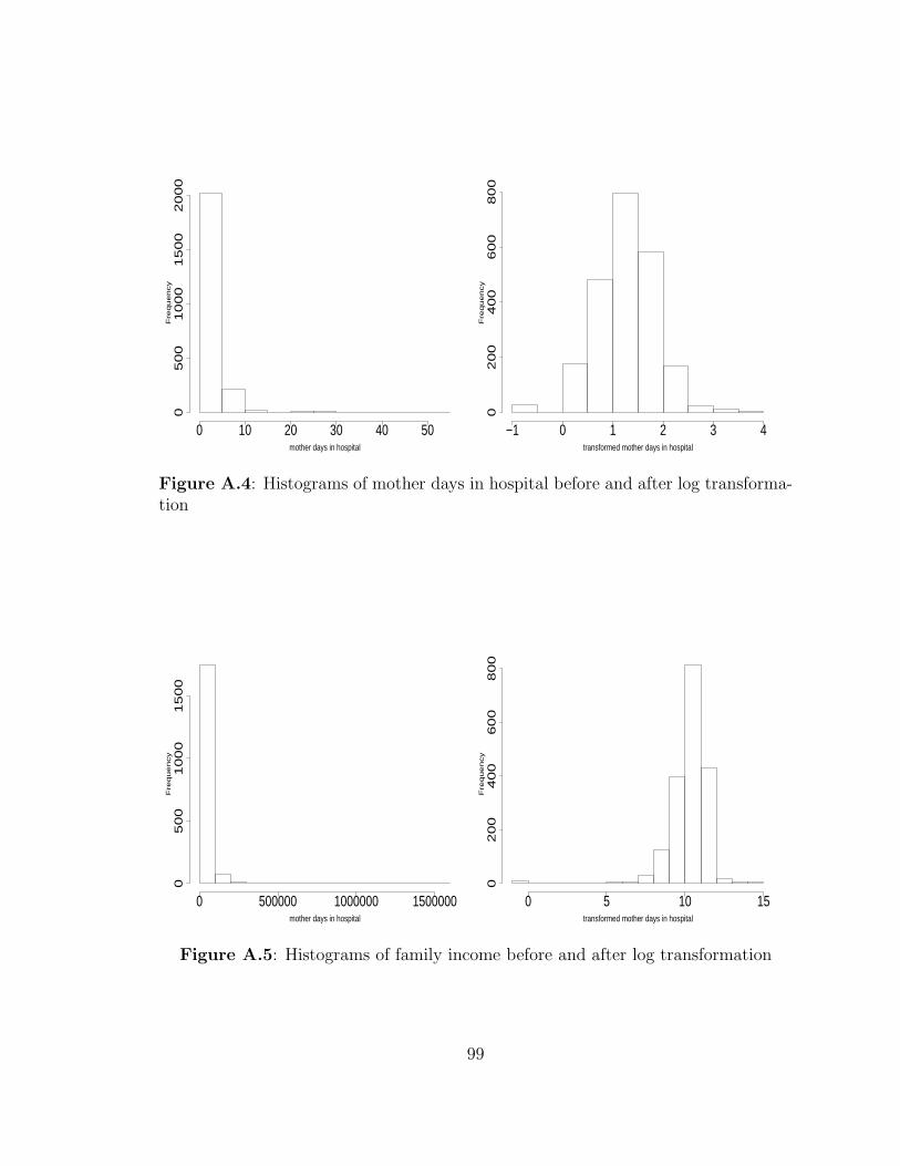
mother days in hospital
Fre
qu
en
cy
0 10 20 30 40 50
05
00
10
00
15
00
20
00
transformed mother days in hospital
Fre
qu
en
cy
−1 0 1 2 3 4
02
00
40
06
00
80
0Figure A.4: Histograms of mother days in hospital before and after log transforma-tion
mother days in hospital
Fre
qu
en
cy
0 500000 1000000 1500000
05
00
10
00
15
00
transformed mother days in hospital
Fre
qu
en
cy
0 5 10 15
02
00
40
06
00
80
0
Figure A.5: Histograms of family income before and after log transformation
99

Appendix B
Appendix to chapter 4 - Full conditionals
We present here the joint posterior distribution and the resulting full conditionals
required for the Gibbs sampler in the SSVS2 approach, focusing for simplicity on the
case in which the response is binary and the predictors are binary or continuous.
SSVS proceeds by sampling from the joint posterior of the model space (γ,γm),
parameters within each model (βγ,φβγ, θγm ,φθγm ,κ), and the latent/unobserved
variables (y∗,X∗,Xmis) conditional on the observed data (y,Xobs). The joint pos-
terior is expressed below,
π(γ, γm, y∗, βγ,φβγ, θγm ,φθγm ,κ,X
∗,Xmis|y,Xobs)
∝∏n
i p(yi|y∗i )p(y∗i |βγ,xi)p(xi, x∗
i |θγm ,κ)
× p(βγ,φβγ|γ)p(γ)π(θγm ,φθγm |γm)p(γm)p(κ)
∝∏n
i
(yiI(y
∗i ≥ 0) + (1 − yi)I(y
∗i < 0)
)N(y∗i ; β0 + x′
γiβγ, 1)
×[∏p
j=1 p(xij |x∗ij)N(x∗ij ; θj0 + x∗
′
jγmj
iθjγmj, κj
)]
×∏p
j=0 p(βj|φβj, γj)p(γj)p(φβj
|γj)
×∏p
j=1
∏j−1k=0
[p(θjk|φθjk
, γmjk)p(φθjk|γmjk)p(γmjk)
]p(κ)
where, p(xij |x∗ij) = xijI(x∗ij ≥ 0) + (1 − xij)I(x
∗ij < 0), κj = 1 for binary xij and
p(xij |x∗ij) = δx∗ij (xij) for continuous xij
With the models for the data and the prior distributions for the parameters dis-
cussed in section 3, the full conditionals are available in closed form. First consider
100

the full conditional distributions for the parameters in the predictor component of
the model. Sample θjk from,
(1 − πjk)δ0 + πjkN(Ejk, Vjk), (B.1)
where the conditional posterior probability of γmjk = 1 is
πjk = 1 − 1 − pjk
1 − pjk + pjk
√φθjk
φ(0)
V−
12
jkφ(V
−12
jkEjk)
,
and the conditional posterior mean and variance given inclusion is
Ejk = Vjkψj
n∑
i=1
x∗ikx∗ijk, Vjk =
(φθjk
+ ψj
n∑
i=1
x∗2
ik
)−1
,
with x∗ijk = x∗ij − θj0 −∑j−1
h=1,h 6=k x∗ihθjh and φ(.) the standard normal density. Also
update φθjkfor predictors included in the model from,
Ga
(1,θ2jk + 1
2
). (B.2)
Next sample ψk = κ−1k for continuous xk from,
Ga
n
2,
(n∑
i=1
x∗ik − (θj0 −k∑
j=1
x∗ijθjk)
)2 (B.3)
while ψk = κ−1k = 1 for binary xk. Now for the ith missing continuous covariate value
xij , we impute from a normal distribution,
N(ψ−1j µij, ψ
−1j
)(B.4)
101

where,
ψj = β2j + ψj +
p∑
k=j+1
ψjθ2kj,
µij = y∗ijβj + ψjµij +
p∑
k=j+1
ψkθkj x∗ikj
and,
y∗ij = y∗i − β0 −∑
h 6=j
xihβh,
µij = θj0 +
j−1∑
k=1
x∗ikθjk,
x∗ikj= x∗ik − θk0 −
k−1∑
h=1,h 6=j
x∗ihθkh.
While when xij is binary and missing, we first impute its underlying latent variable
x∗ij from the full conditional,
πijN+
(ψ−1j µij , ψ
−1j
)+ (1 − πi)N−
(ψ−1j µij, ψ
−1j
)(B.5)
where,
ψ−1j = ψj +
p∑
k=j+1
ψjθ2kj ,
µij = ψjµij +
p∑
k=j+1
ψkθkjx∗ikj,
πij =
(1 − Φ
(µij√ψj
))φ(y∗ij − βj
)
(1 − Φ
(µij√ψj
))φ(y∗ij − βj
)+ Φ
(µij√ψj
)φ(y∗ij
)
102

and,
µij = θj0 +
j−1∑
k=1
x∗ikθjk,
x∗ikj= x∗ik − θk0 −
k−1∑
h=1,h 6=j
x∗ihθkh,
y∗ij = y∗i − β0 −∑
h 6=j
xihβh,
and then impute xij = I(x∗ij > 0). We also update latent x∗ij for observed binary xij
from the following distribution:
xijN+
(ψ−1j µij, ψ
−1j
)+ (1 − xij)N−
(ψ−1j µij, ψ
−1j
)(B.6)
where, ψ and µij are as in (B.5). Note that for individual i predictors other than
xij may be missing, in the imputations we condition on the most recently imputed
values of other missing predictors. Now conditional on the observed and imputed
predictors we can sample from the full conditionals in the top level models for the
response. We sample βj from its full conditional posterior,
(1 − πj)δ0 + πjN(Ej , Vj), (B.7)
where πj is the conditional posterior probability of γj = 1, which is
πj = 1 − 1 − πj
1 − πj + πj
√φβj
φ(0)
V−
12
j φ(V−
12
j Ej)
,
103

and the conditional expectation and variance of βj given γj = 1 are
Ej = Vj
n∑
i=1
xij y∗ij, Vj =
(φβj
+n∑
i=1
x2ij
)−1
,
with y∗ij = y∗i − β0 −∑
h 6=j xihβh and φ(.) the standard normal density. We sample
φβjfor predictors included in the model from its full conditional,
Ga
(1,β2j + 1
2
). (B.8)
Finally sample y∗i from its full conditional,
yiN+(x′
iβ, 1) + (1 − yi)N−(x′
iβ, 1) (B.9)
In this way within one Gibbs sampler we repeatedly impute values for the missing
covariates from their full conditional distributions and conditional on the completed
data set perform variable selection on the model relating the response to the predic-
tors.
When imputing missing values in the out of sample test data we do not observe the
response y and so we must impute from modified full conditionals. For xij missing
and continuous impute from,
N(ψ−1j µij, ψ
−1j
)(B.10)
where, ψj and µij are as in (B.5). For xij missing and binary impute its underlying
latent variable x∗ij from (B.10) and impute xij = I(x∗ij > 0). For xij observed and
binary update x∗ij from the same distribution as (B.6).
104

Bibliography
AAP (2005). Breastfeeding and the use of human milk. Pediatrics 115, 496–506.
Albert, J. H. and Chib, S. (1993). Bayesian analysis of binary and polychotomousresponse data. Journal of the American Statistical Association 88, 669–679.
Barnard, J. and Rubin, D. B. (1999). Small-sample degrees of freedom with multiple-imputation. Biometrika 86, 948–955.
Beunckens, C., Molenberghs, G., Verbeke, G., and Mallinckrodt, C. (2008). A latent-class mixture model for incomplete longitudinal gaussian data. Biometrics 64,96–105.
Box, G. E. P. and Cox, D. R. (1964). An analysis of transformations. Journal of theRoyal Statistical Society. Series B (Methodological) 26, 2, 211–252.
Cai, B. and Dunson, D. (2006). Bayesian covariance selection in generalized linearmixed models. Biometrics 62, 446–457.
Clyde, M. and George, E. (2004). Model uncertainty. Statistical Science 19, 81–94.
Cochran, W. (1953). Matching in analytical studies. American Journal of PublicHealth 43, 684–691.
Cochran, W. G. and Chambers, S. P. (1965). The planning of observational studiesof human populations. Journal of the Royal Statistical Society. Series A (General)128, 2, 234–266.
D’Agostino, R. B. (1998). Propensity score methods for bias reduction in the com-parison of a treatment to a non-randomized control group. Statistics in Medicine17, 2265–2281.
D’Agostino, R. B. J. and Rubin, D. B. (2000). Estimating and using propensityscores with partially missing data. Journal of the American Statistical Association95, 451, 749–759.
Der, G., Batty, G. D., and Deary, I. J. (2006). Effect of breast feeding on intelligencein children: prospective study, sibling pairs analysis, and meta-analysis. BMJ 333.
Diamond, A. and Sekhon, J. (2005). Genetic matching for estimating causal effects.presented at the Society for Political Methodology Meeting, FSU, July 21-23 2005.
Diebolt, J. and Robert, C. P. (1994). Estimation of finite mixture distributionsthrough bayesian sampling. Journal of the Royal Statistical Society. Series B(Methodological) 56, 2, 363–375.
105

Drake, C. (1993). Effects of misspecification of the propensity score on estimators oftreatment effect. Biometrics 49, 1231–1236.
Eastaugh, J., Smye, S., Snowden, S., Walker, J., Dear, P., and Farrin, A. (1997).Comparison of neural networks and statistical models to predict gestational age atbirth. Neural Computing & Applications 6, 158–164.
Fay, R. E. (1996). Alternative paradigms for the analysis of imputed survey data.Journal of the American Statistical Association 91, 490–498.
Gelman, A., Carlin, J. B., Stern, H. S., and Rubin, D. B. (1995). Bayesian DataAnalysis. London: Chapman & Hall.
George, E. and McCulloch, R. (1993). Variable selection via gibbs sampling. Journalof the American Statistical Association 88, 881–889.
George, E. and McCulloch, R. (1997). Approaches for bayesian variable selection.Statistica Sinica 7, 339–373.
Hill, J. (2004). Reducing bias in treatment effect estimation in observational studiessuffering from missing data. Columbia University Institute for Social and EconomicResearch and Policy (ISERP) working paper 04-01.
Hill, J. and Reiter, J. P. (2006). Interval estimation for treatment effects usingpropensity score matching. Statistics in Medicine 25, 2230–2256.
Hill, J. L. and McCulloch, R. E. (2007). Bayesian nonparametric modeling for causalinference. University of Chicago Graduate School of Business working paper.
Hoeting, J. A., Madigan, D., Raftery, A. E., and Volinsky, C. T. (1999). Bayesianmodel averaging: A tutorial. Statistical Science 14, 382–401.
Horvitz, D. G. and Thompson, D. J. (1952). A generalization of sampling withoutreplacement from a finite universe. Journal of the American Statistical Association47, 260, 663–685.
Ibrahim, J., Lipsitz, S., and Chen, M.-H. (1999). Missing covariates in generalizedlinear models when the missing data mechanism is nonignorable. Journal of theRoyal Statistical Society, Ser. B 61, 173–190.
Kinney, S. K. and Dunson, D. (2007). Fixed and random effects selection in linearand logistic models. Biometrics 63, 690–698.
Lavori, P. W., Keller, M. B., and Endicott, J. (1995). Improving the aggregateperformance of psychiatric diagnostic methods when not all subjects receive thestandard test. Statistics in Medicine 14, 1913–1925.
106

Lechner, M. (1999). Earnings and employment effects of continuous off-the-job train-ing in east germany after unification. Journal of Business and Economic Statistics17, 1, 74–90.
Li, K.-H. (1988). Imputation using Markov chains. Journal of Statistical Computationand Simulation 30, 57–79.
Li, K. H., Raghunathan, T. E., Meng, X. L., and Rubin, D. B. (1991). Significancelevels from repeated p-values with multiply-imputed data. Statistica Sinica 1,65–92.
Liang, F., Paulo, R., Molina, G., Clyde, M. A., and Berger, J. (2008). Mixturesof g Priors for Bayesian Variable Selection. Journal of the American StatisticalAssociation 103, 410–423.
Lipsitz, S. and Ibrahim, J. (1996). A conditional model for incomplete covariates inparametric regression models. Biometrika 83, 916–922.
Little, R. J. A. (1993). Pattern-mixture models for multivariate incomplete data.Journal of the American Statistical Association 88, 125–134.
Little, R. J. A. (1994). A class of pattern-mixture models for normal incompletedata. Biometrika 81, 471–483.
Little, R. J. A. and Rubin, D. B. (2002). Statistical Analysis with Missing Data:Second Edition. New York: John Wiley & Sons.
Little, R. J. A. and Schluchter, M. D. (1985). Maximum likelihood estimation formixed continuous and categorical data with missing values. Biometrika 72, 497–512.
Little, R. J. A. and Wang, Y. (1996). Pattern-mixture models for multivariate in-complete data with covariates. Biometrics 52, 98–111.
Lohr, S. L. (1999). Sampling: Design and Analysis. Duxbury Press.
Longnecker, M. P., Klebanoff, M. A., Zhou, H., and Brock, J. W. (2001). Associationbetween maternal serum concentration of the ddt metabolite dde and preterm andsmall-for-gestational-age babies at birth. Lancet 358, 110–114.
Lu, B., Zanutto, E., Hornik, R., and Rosenbaum, P. R. (2001). Matching with dosesin an observational study of a media campaign against drug abuse. Journal of theAmerican Statistical Association 96, 456, 1245–1253.
Lunceford, J. and Davidian, M. (2004). Stratification and weighting via the propen-sity score in estimation of causal treatment effects: a comparative study. Statisticsin Medicine 23, 2937–2960.
107

Madigan, D. and York, J. (1995). Bayesian graphical models for discrete data. In-ternational Statistical Review / Revue Internationale de Statistique 63, 215–232.
McCandless, L. C., Gustafson, P., and Austin, P. C. (2008). Bayesian propensityscore analysis for observational data. Statistics in Medicine Accepted.
Meng, X.-L. (1994). Multiple-imputation inferences with uncongenial sources of input(disc: P558-573). Statistical Science 9, 538–558.
Meng, X. L. and Rubin, D. B. (1992). Performing likelihood ratio tests with multiply-imputed data sets. Biometrika 79, 103–111.
Mengersen, K. L. and Robert, C. P. (1996). Testing for mixtures: A Bayesian entropicapproach. In J. M. Bernardo, J. O. Berger, A. P. Dawid, and A. F. M. Smith, eds.,Bayesian Statistics 5 – Proceedings of the Fifth Valencia International Meeting,255–276. Clarendon Press (Oxford University Press).
Mitchell, T. and Beauchamp, J. (1988). Bayesian variable selection in linear regres-sion. Journal of the American Statistical Association 83, 1023–1032.
Olkin, I. and Tate, R. F. (1961). Multivariate correlation models with mixed discreteand continuous variables. The Annals of Mathematical Statistics 32, 2, 448–465.
Raftery, A. (1996a). Approximate bayes factors and accounting for model uncertaintyin generalised linear models. Biometrika 83, 251–266.
Raftery, A. (1996b). Hypothesis testing and model selection via posterior simulation.In Practical Markov Chain Monte Carlo (eds W.R. Gilks, D.J. Spiegelhalter andS. Richardson), 163–188. London: Chapman and Hall.
Raftery, A., Madigan, D., and Hoeting, J. (1997). Bayesian model averaging for linearregression models. Journal of the American Statistical Association 92, 179–191.
Raghunathan, T. E., Lepkowski, J. M., van Hoewyk, J., and Solenberger, P. (2001).A multivariate technique for multiply imputing missing values using a series ofregression models. Survey Methodology 27, 85–96.
Rao, J. N. K. (1996). On variance estimation with imputed survey data. Journal ofthe American Statistical Association 91, 499–506.
Rao, J. N. K. and Shao, J. (1992). Jackknife variance estimation with survey dataunder hot deck imputation. Biometrika 79, 4, 811–822.
Reiter, J. P. (2007). Small-sample degrees of freedom for multi-component significancetests with multiple imputation for missing data. Biometrika 94, 502–508.
108

Richardson, S. and Green, P. J. (1997). On bayesian analysis of mixtures with anunknown number of components. Journal of the Royal Statistical Society. SeriesB (Methodological) 59, 4, 731–792.
Roeder, K. and Wasserman, L. (1997). Practical Bayesian density estimation usingmixtures of normals. Journal of the American Statistical Association 92, 894–902.
Rosenbaum, P. R. (1991). A characterization of optimal designs for observationalstudies. Journal of the Royal Statistical Society, Series B-Methodological 53, 597–610.
Rosenbaum, P. R. and Rubin, D. B. (1983). The central role of the propensity scorein observational studies for causal effects. Biometrika 70, 41–55.
Rosenbaum, P. R. and Rubin, D. B. (1984). Reducing bias in observational studiesusing subclassification on the propensity score. Journal of the American StatisticalAssociation 79, 516–524.
Rosenbaum, P. R. and Rubin, D. B. (1985a). The bias due to incomplete matching.Biometrics 41, 1, 103–116.
Rosenbaum, P. R. and Rubin, D. B. (1985b). Constructing a control group usingmultivariate matched sampling methods that incorporate the propensity score.The American Statistician 39, 1, 33–38.
Rubin, D. (1974). Estimating causal effects of treatments in randomized and non-randomized studies. Journal of Educational Psychology 66, 5, 688–701.
Rubin, D. (1976). Inference and missing data. Biometrika 63, 3, 581–592.
Rubin, D. (1978a). Bayesian inference for causal effects: The role of randomization.The Annals of Statistics 6, 1, 34–58.
Rubin, D. B. (1978b). Multiple imputations in sample surveys: A phenomenologicalBayesian approach to nonresponse (C/R: P29-34). In ASA Proceedings of theSection on Survey Research Methods, 20–28. American Statistical Association.
Rubin, D. B. (1986). Basic ideas of multiple imputation for nonresponse. SurveyMethodology 12, 37–47.
Rubin, D. B. (1987). Multiple Imputation for Nonresponse in Surveys. Wiley.
Rubin, D. B. (1996). Multiple imputation after 18+ years. Journal of the AmericanStatistical Association 91, 473–489.
Rubin, D. B. and Schenker, N. (1986). Multiple imputation for interval estimationfrom simple random samples with ignorable nonresponse. Journal of the AmericanStatistical Association 81, 394, 366–374.
109

Schafer, J. L. (1997). Analysis of Incomplete Multivariate Data. London: Chapman& Hall.
Schafer, J. L. (1999). NORM: Multiple imputation of incomplete multivariate dataunder a normal model [Computer software]. University Park: Pennsylvania StateUniversity, Department of Statistics.
Schafer, J. L. and Graham, J. W. (2002). Missing data: Our view of the state of theart. Psychological Methods 7, 147–177.
Shao, J., Chen, Y., and Chen, Y. (1998). Balanced repeated replications for stratifiedmultistage survey data under imputation. Journal of the American StatisticalAssociation 93, 819–831.
Sianesi, B. (2004). An evaluation of the swedish system of active labor market pro-grams in the 1990s. Review of Economics and Statistics 86, 1, 133–155.
Tanner, M. A. and Wong, W. H. (1987). The calculation of posterior distributions bydata augmentation. Journal of the American Statistical Association 82, 528–540.
Vikram, H. R., Buenconsejo, J., Hasbun, R., and Quagliarello, V. J. (2003). Impactof Valve Surgery on 6-Month Mortality in Adults With Complicated, Left-SidedNative Valve Endocarditis: A Propensity Analysis. JAMA 290, 24, 3207–3214.
Wasserman, L. (2000). Asymptotic inference for mixture models by using data-dependent priors. Journal of the Royal Statistical Society: Series B (StatisticalMethodology) 62, 1, 159–180.
Yang, X., Bellin, T., and Boscardin, W. (2006). Imputation and variable selection inlinear regression models with missing covariates. Biometrics 61, 498–506.
York, J., Madigan, D., Heuch, I., and Lie, R. T. (1995). Estimating a proportionof birth defects by double sampling: a Bayesian approach incorporating covariatesand model uncertainty. J. Roy. Statist. Soc. Ser. C 44, 227–242.
110

Biography
Robin obtained his BSc in Mathematics, Operations Research, Statistics and Eco-
nomics from Warwick University in 2004. He obtained his M.S. from Duke University
in 2006. He has co-authored the following articles:
1. Reiter JP and Mitra R. “Estimating risks of identification disclosure in partially
synthetic data.” Journal of Privacy and Confidentiality (Accepted 2007)
2. Mitra R and Reiter JP. “Adjusting survey weights when altering identifying
design variables via synthetic data.” Privacy in Statistical Databases. Ed. J
Domingo Ferrer and L Franconi, Lecture Notes in Computer Science, Springer
2006: 177-188
111