MASTER THESIS

Bayesian Mixed Integer Optimization Using A-Priori Knowledge on Variable Dependences

Anyi ZHANG ( 0625898)

Supervisor : Dr. Michael T. M. Emmerich

Drs. Rui Li

1

OUTLINE Abstract

Chapter 1 Introduction

Chapter 2 Algorithms

Chapter 3 Artificial Test Problems

Chapter 4 Experiments and Results

Chapter 5 Summary and Outlook

References

Acknowledgements

2

ABSTRACT Mixed-integer optimization problems arise in various application fields, such as optical filtering, chemical engineering and medical image processing. The variables to optimize are not always independent to each other. This work aims to find good solution methods for this category of problems. Stochastic optimization algorithms can be used as solution methods for solving these problems approximately. Especially for real-world problems they often prove to be powerful due to their flexibility and robustness. Recently a well-tuned mixed integer optimization algorithm, Mixed-Integer Evolutionary Strategy (MIES) has been developed and applied to chemical plant engineering as well as medical image processing. But it has the limitation of not being able to learn variable dependences. We thus consider estimation of distribution algorithms (EDAs) which use probabilistic models to replace the population in classical EAs. Being one of the earliest EDAs, population based incremental learning (PBIL) works under the assumption of variable independency and therefore is incapable of grasping the relation between variables. In comparison, Bayesian Optimization Algorithms (BOA) can explore variable dependences. It makes progress by repeatedly learning a Bayesian network from the 'good' individuals and then sampling the resulting model. A-priori information on variable dependences can be easily coupled. In this work, both the two algorithms are extended to deal with variables of mixed type. As a proof of concept study, we apply them, together with MIES, to ADG-based mixed-integer NK Landscapes. The statistical results obtained are very encouraging.

KEYWORDS Mixed-Integer Optimization; Population-based Incremental Learning; ADG-based NK Landscapes; Medical Image Processing; Bayesian networks; Bayesian Optimization Algorithm

3

Chapter 1 Introduction We study solution methods for difficult optimization problems where decision variables are of different type and not independent to each other. In particular we look at problems where the decision vector consists of continuous, ordinal and nominal discrete variables. This work is triggered by many real-world problems like the optical filtering, chemistry plant engineering [12] and medical image processing[20], etc. The optimization of the IVUS (intravascular ultrasound) lumen detection pipeline (Figure 1) is an example in medical image processing field.

IVUS images show the inside of coronary arteries and are acquired with an ultrasound catheter positioned inside the vessel. Effective detection of structures is desired for clinical diagnosis. Considering the huge work and inaccuracy of manual segmentation, an multi-agent automatic system (Figure 1) is developed, consisting of multiple agents among which is the lumen agent. Lumen agent holds many feature detectors (Figure 2) therefore a large number of parameters (Table 1) to optimize for the image at hand. However these parameters are hard to optimize manually and may differ for different interpretations. In addition, these parameters are of different type (nominal discrete, continuous or integer) and since some relationship has been built up between them by construction of the processing pipeline they are not independent to each other. In this sense the setting of the parameters of the pipeline is essentially a mixed-integer multivariate optimization problem. Works have been done to optimize these parameters using evolutionary strategies (EAs). Among them, MIES[20]proves to be significantly more effective than others.

However, as a member of classical EAs the searching mechanics of MIES is fixed and problem-independent which means the structure of problem on the fly is ignored. On the other hand, the structure of the IVUS optimization problem is quite obvious, defined by the pipeline. Therefore we think MIES is not the best choice in this case and try to find alternatives in another class of EAs, the estimation of distribution algorithms (EDAs) which try to model the distributions of solutions in search space.

Figure 1: coronary vessel image processing multi-agent system.

1

Figure 2: IVUS lumen detection pipeline.

Table 1: parameters for the lumen feature detector.

name type range dependences default

maxgray

mingray

connectivity

relativeopenings

nrofcloses

nrofopenings

scanlinedir

scanindexleft

scanindexright

centermethod

fitmodel

sigma

scantype

sidestep

sidecost

nroflines

integer

integer

nominal

boolean

integer

integer

nominal

integer

integer

nominal

nominal

continuous

nominal

integer

continuous

integer

[2, 150]

[1, 149]

{4,6,8}

{false,true}

[0, 100]

[0, 100]

{0,1,2}

[-100, 100]

[-100, 100]

{0,1}

{ellipse, circel}

[0.5 10.0]

{0,1,2}

[0, 20]

[0.0, 100]

[32, 256]

> mingray

< maxgray

Used if not relativeopenings

Used if not relativeopenings

< scanindexright

> scanindexleft

35

1

6

true

5

45

1

-55

7

1

ipse

0.8

0

3

5

128

2

3

Population-Based Incremental Learning (PBIL) is a well-known EDA which “removes the genetics from the genetic algorithm”[23]. Unlike classical EAs working on low-level representations, trying to create better individuals by directly recombinating and mutating the individuals, PBIL employs a probabilistic model, which is the only persistent part of the search process [2, 3], as the high-level abstraction of the search space and guides the search by updating the model. Probabilistic model is built on the statistical information contained in selected individuals and can be considered as the estimation of the structure of them. Originally PBIL is designed for binary search spaces, but has been extended to continuous spaces by utilizing different methods and models like the interval approach[7], the Gaussian distribution model [14] and the histogram-based model[1]. In this work, we will extend it to mixed-integer case.

However in PBIL, to estimate of the structure of good individuals we assume a distribution for each gene separately and no mutual information between genes considered which can be addressed given joint distribution of genes estimated instead. Actually, in continuous domain, algorithms like UMDA fall into the same category. They all assume solution variables are independent to each other and construct the model with univariate distributions. In comparison, MIMIC, LFDA, ECGA and BOA take the variable dependences into consideration by defining a joint probability distribution and are expected to be better options for problems with obvious variable dependency [16]BOA especially excites our interest as it can be extended to deal with different types of variables and can easily couple a-priori information of problem structure. In [13], binary BOA has been studied and proved to possess good properties: it identifies, reproduces, and mixes building blocks to a specified order and is independent of dimension of the problem. We extend it to mixed-integer case and test its performance in this domain.

To test the abovementioned three algorithms, MIES, PBIL and BOA, artificial landscapes with scalable ruggedness designed specially for study of gene interactions, namely NK Landscapes[10] are used. NK Landscapes were proposed by Kauffman[22]. Studies have been done of different aspects: property of itself, computation complexity of optimization and also the behavior of classical EAs on it. Recently it has been extended to mixed-integer case[19]. In our work we further introduce dependences between genes defined by an Acyclic Directed Graph (ADG) into the construction of it and get so-called ADG-based mixed-integer NKL for our use.

The paper is organized as follows. In Chapter 2, all three algorithms, MIES, PBIL and BOA are reviewed and the latter two are extended to integer case. Chapter 3 reviews basic concepts of NKL, its extension to mixed-integer case, and then introduces the construction of ADG-based mixed-integer NKL (MI-NKL). Chapter 4 reports on experimental results. The paper ends with a summary of our work and a brief outlook of future work.

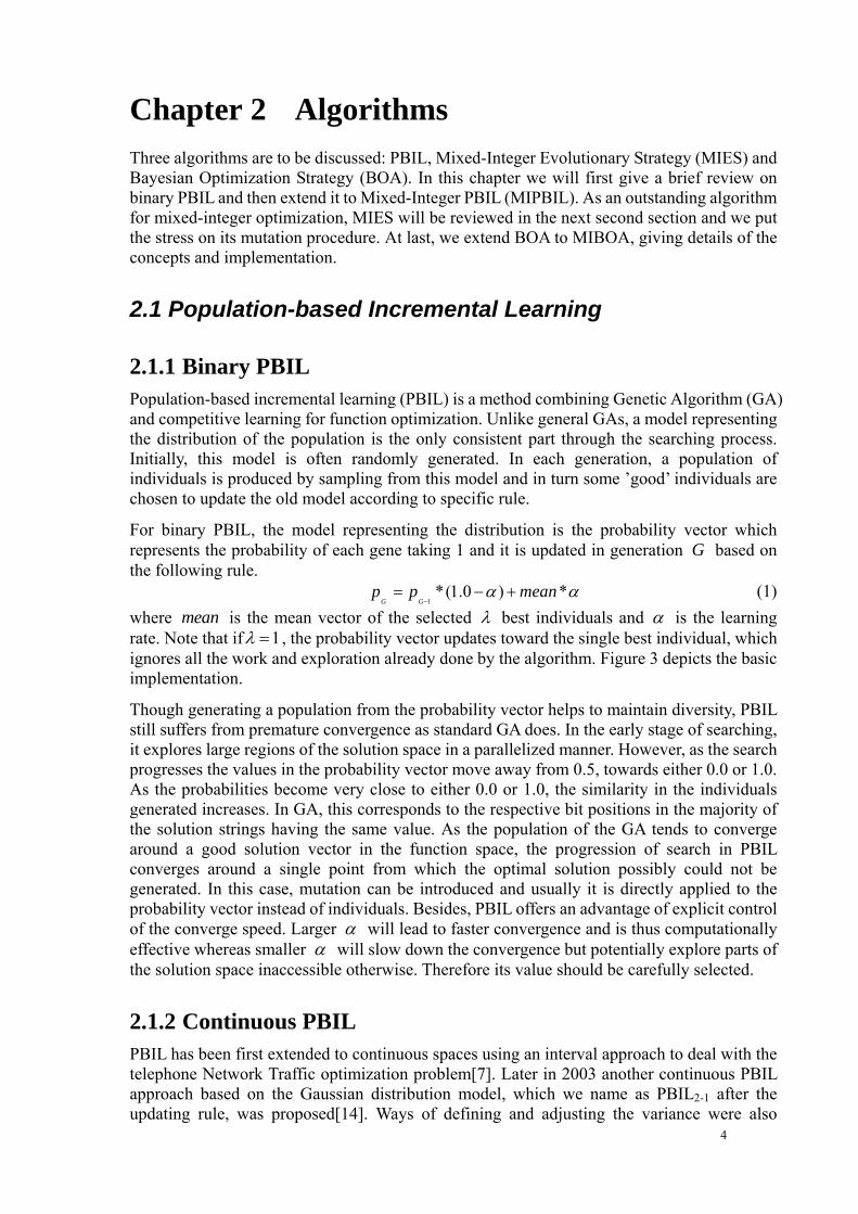
Chapter 2 Algorithms Three algorithms are to be discussed: PBIL, Mixed-Integer Evolutionary Strategy (MIES) and Bayesian Optimization Strategy (BOA). In this chapter we will first give a brief review on binary PBIL and then extend it to Mixed-Integer PBIL (MIPBIL). As an outstanding algorithm for mixed-integer optimization, MIES will be reviewed in the next second section and we put the stress on its mutation procedure. At last, we extend BOA to MIBOA, giving details of the concepts and implementation.

2.1 Population-based Incremental Learning

2.1.1 Binary PBIL Population-based incremental learning (PBIL) is a method combining Genetic Algorithm (GA) and competitive learning for function optimization. Unlike general GAs, a model representing the distribution of the population is the only consistent part through the searching process. Initially, this model is often randomly generated. In each generation, a population of individuals is produced by sampling from this model and in turn some ’good’ individuals are chosen to update the old model according to specific rule.

For binary PBIL, the model representing the distribution is the probability vector which represents the probability of each gene taking 1 and it is updated in generation based on the following rule.

G

1*(1.0 ) *

G Gp p meanα α

−= − + (1)

where is the mean vector of the selected mean λ best individuals and α is the learning rate. Note that if 1λ = , the probability vector updates toward the single best individual, which ignores all the work and exploration already done by the algorithm. Figure 3 depicts the basic implementation.

Though generating a population from the probability vector helps to maintain diversity, PBIL still suffers from premature convergence as standard GA does. In the early stage of searching, it explores large regions of the solution space in a parallelized manner. However, as the search progresses the values in the probability vector move away from 0.5, towards either 0.0 or 1.0. As the probabilities become very close to either 0.0 or 1.0, the similarity in the individuals generated increases. In GA, this corresponds to the respective bit positions in the majority of the solution strings having the same value. As the population of the GA tends to converge around a good solution vector in the function space, the progression of search in PBIL converges around a single point from which the optimal solution possibly could not be generated. In this case, mutation can be introduced and usually it is directly applied to the probability vector instead of individuals. Besides, PBIL offers an advantage of explicit control of the converge speed. Larger α will lead to faster convergence and is thus computationally effective whereas smaller α will slow down the convergence but potentially explore parts of the solution space inaccessible otherwise. Therefore its value should be carefully selected.

2.1.2 Continuous PBIL PBIL has been first extended to continuous spaces using an interval approach to deal with the telephone Network Traffic optimization problem[7]. Later in 2003 another continuous PBIL approach based on the Gaussian distribution model, which we name as PBIL2-1 after the updating rule, was proposed[14]. Ways of defining and adjusting the variance were also

4

investigated and the best option appeared to be learning the variance in the same way as the center of the distribution. The results presented in [14] pointed out the limitation of PBIL2-1 and improved it with a new updating rule which takes all the individuals into account and a self-adaptive learning rate. Furthermore, it proposed to replace the Gaussian model with a histogram-based probabilistic model which depicts the distribution of ‘good’ solutions in a more accurate way but inevitably introduces more complexity. Thus it is excluded from our consideration.

p ← initialize probability vector (each position = 0.5)

Loop # GENERATIONS

#Generate population of sizeµ

i ← loop #INDIVIDUALS

Generate(individual ); i

Evaluate(population ); i

#find best individuals and calculate their mean

sePop←Select(bestλ individuals);

m←mean(sePop);

#update probability vector

j ← loop #LENGTH

*(1.0 ) *j j jp p mα α← − +

#mutate probability vector

j ← loop #LENGTH

*(1.0 ) ({0,1})*j jp p MUT U MUT← − +

Generate(individual ) i

j ← loop #LENGTH

if (U(0,1)< jp ) locus = 1; j

Otherwise locus = 0; j

USER DEFINED CONSTANTS:

GENERATIONS: number of iterations to allow learning

INDIVIDUALS: the population size, number of samples to produce per generation

LENGTH: length of encoded solution (dimension)

MUT: amount for mutation to affect the probability vector

α : learning rate

VARIABLES: p : Probability vector

Figure 4: The basic PBIL.Note means uniformly randomly selecting an element out of{0 . ({0,1})U ,1}

5

2.1.3 Extension to Mixed-Integer PBIL

To extend PBIL to Mixed-integer case, the key is to find efficient measurements (module) for different type of genes. For a nominal discrete gene, the frequency of taking each value describes the distribution therefore a probability vector should be introduced for each locus:

, where represents the probability that locus takes the value. i ij p =(p ), j=1 LL ijp i 'j th

6

Figure 5: The PBIL representation of population.

As for continuous variable, we assume it follows a normal distribution. Then two parameters need to be considered and updated in each generation, that is, mean and standard deviation

mσ .

Things become more complex for integer genes. One option is to take it as a special case of continuous variable and assume normal distribution. However, a more reasonable assumption for integer variables is geometric distribution which has properties similar to normal distribution: unimodal, with a peak at zero and infinite support in Z. The only parameter p , representing the probability of succeed in one Bernoulli trial, indirectly controls the standard deviation. Moreover, as pointed out in [6], multivariate geometric distribution is characterized by a rotational symmetry with regard to the norm and belongs to a family of maximal entropy distributions. All these characteristics make the geometric distribution well suited for integer programming. As we will see, MIES uses it well. However, in PBIL, there exists difficulty updating the only parameter

1L

p directly from ‘good’ solution. Thus we take a way in between: update and m σ for integer variables just like in continuous case but generate geometrical distributed instantiations(Figure 3). This can be done as follows.

1 2G = m + * (G ( 3-1)- G ( 3-1)σ ） (2) Where , are geometrically distributed random numbers that can be generated from two uniformly distributed random variables

1G 2G

1 2: (0,1); : (0,1u U u U )= = via

1 2ln(1 ), ,ln(1 )

ii

uG G G G ip

1, 2−= − = =

− (3)

2.2 Mixed-Integer Evolutionary Strategy

Mixed-Integer Evolution Strategy (MIES) was first proposed by Emmerich et al. for chemical engineering plant optimization with process simulators from industry [12] and was adapted by

Equivalent PBIL representation Probability distribution stores information about frequency of values at each allele. Alleles Number: 1 2 3 4 5 6 7

A= 0.2 0.2 0.6 0.4 0.8 0.4 0.6B=0.2 0.6 0.4 0.6 0.0 0.6 0.2C=0.6 0.0 0.0 0.0 0.2 0.0 0.2

⎧⎪⎨⎪⎩

GA representation Alleles number:1 2 3 4 5 6 7

⎧⎪⎪⎪⎨⎪⎪⎪⎩

GA

population

A B A B A B AC B A A A B AB A B A A B BC B B A C A AC A A B A A C

Value Frequenc

F

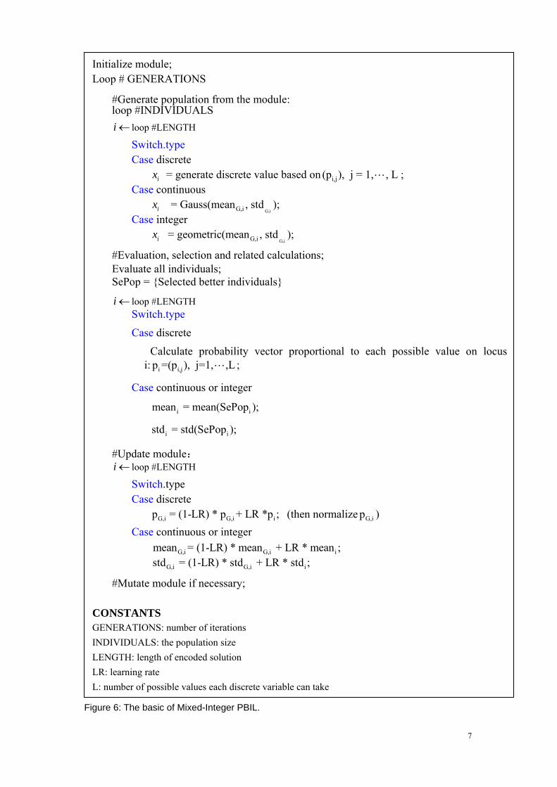
Initialize module; Loop # GENERATIONS

#Generate population from the module: loop #INDIVIDUALS i ← loop #LENGTH

Switch.type Case discrete

ix = generate discrete value based on i,j(p ), j = 1, , L ;L

Case continuous ix

G,iG,i= Gauss(mean , std ); Case integer

ix G,iG,i= geometric(mean , std );

#Evaluation, selection and related calculations; Evaluate all individuals; SePop = {Selected better individuals}

i ← loop #LENGTH Switch.type

Case discrete

Calculate probability vector proportional to each possible value on locus i: ; i i,jp =(p ), j=1, ,LL

Case continuous or integer

i imean = mean(SePop );

i istd = std(SePop );

#Update module： i ← loop #LENGTH

Switch.type Case discrete

G,i G,i ip = (1-LR) * p + LR *p ; (then normalize p ) G,i

Case continuous or integer

G,i G,i imean = (1-LR) * mean + LR * mean ; G,i G,i istd = (1-LR) * std + LR * std ;

#Mutate module if necessary; CONSTANTS GENERATIONS: number of iterations INDIVIDUALS: the population size LENGTH: length of encoded solution LR: learning rate L: number of possible values each discrete variable can take

igure 6: The basic of Mixed-Integer PBIL.

7

Figure 7: Mutation procedure in MIES. Courtesy of Li et al[20].

Li. et al[20]. It can deal with continuous, integer and nominal discrete variables simultaneously. In MIES, individuals are represented as tuples 1 1 1( , ,

r zn nr r z z d dL L L ,dn

)n1 1 1, ,pn n p p

σ ζσ σ ζ ζL L L taken from the search space S. While

are object parameters, 1 1 1( , ,

r zn nr r z z d dL L L )dn

)n1 1 1( , ,pn n p p

σ ζσ σ ζ ζL L L are called strategy parameters and their

explicit explanations are that 1 , nσσ σL are standard deviation of the step-sizes for the

continuous variables, 1 , nζζ ζL are mean step-sizes for the geometrical distribution for the

ordinal discrete variables, and 1 ,pnp pL are mutation probabilities for the nominal discrete

variables. The generational loop of the MI-ES reads as follows: After random initialization and evaluation of µ individuals, λ offspring individuals are generated through a recombination and a mutation operator. Then the fitness function is used to evaluate theseλ offspring. Next, the selection operator chooses the µ best individuals among thoseλ offspring individuals and µ parental individuals that do not exceed the maximal life-span (age). Usually, life-span or age is expressed using , and corresponds to ak k = 1 ( , )µ λ -selection and to a k = ∞ ( + )µ λ selection. As long as the termination criterion is not fulfilled, the µ selected individuals form the parental generation for the next iteration loop. To allow for an automatic step-size adaptation it is recommended to set / 7µ λ ≥ and use a comma-strategy.

In MIES, operators work on both the object variables and step sizes. The recombination operator used is similar to the standard recombination in ES: uniform crossover (deterministic recombination) for the object variables and intermediate recombination for the step-size variables. However the mutation procedure differs by taking into account the type of objective variables as detailed in Figure 6. The recommended setting for the local and global step-size

learning rates lτ and gτ are 1 2l rnτ = and 1 2l rnτ = . If 0lτ = , then all variables take 8

the same step size and it is a single step-size strategy. As the algorithm progresses, the step sizes are automatically adapted and tend to decrease gradually. Remark that treating the integer variables simply as truncation of continuous variables is risky as the step sizes might decrease to small values after a number of iterations, too small to generate any alternation of the search point. That is one of the reasons integer variables are mutated by geometric numbers in MIES. And the geometrically distributed random number is generated the way in (3) where is defined by

p

iζ .

2 1/ 21(1 ( ) ) 1

i d

i d

npn

ζζ

= −+ +

Here iζ represents the mean step size for integer variables and in implementation it is forced to be no smaller than 1 in order to avoid stagnation. In [20], MIES was applied to both artificial problem and IVUS pipeline optimization and it is proved to be significantly more effective than standard ES. More details of the algorithm and its implementation can be found in [12] and [20].

2.3 Bayesian Optimization Algorithm

A Bayesian network is a graphical representation of a probabilistic problem, formally defined as a pair , where is the joint probability distribution on the set of random variables and G is an Acyclic Directed Graph (ADG) representing the dependence and independence relations among this set of random variables, where each graphically represented marginal and conditional independence also has to be valid in the joint probability distribution[8]. Denote

B = (G, P) P

1( , )NX X X= L the set of random variables. Then based on the independence relations in the graph , a Bayesian network encodes a joint probability distribution, which can be factorized as

G

1

( ) ( ( ))N

ii

P x p x parent x=

=∏ i (4)

where ( )iparent X is the graphically represented set of parents of iX . It implies that a joint probability distribution can be defined in terms of local distributions, resulting in significant computational savings.

The key of the popularity of Bayesian networks is their ease of representation of independence relations, and their support for reasoning with uncertainty. For reasoning in Bayesian networks there are several exact methods proposed that make use of local computations [18]. However, the correctness of the inference method depends on the type of the parents of a variable and on the choice of the local probability distribution. For example, the method introduced by Lauritzen [24], using exact inference that is based on a conditional Gaussian distribution but it has the restriction that discrete random variables are not allowed to have continuous parents when hybrid Bayesian networks[1] are concerned. To overcome this problem, Koller proposed a method which defines the distribution of these discrete nodes by a mixture of exponentials. However, for the inference it uses Monte Carlo methods[3]. Another solution to this problem is to discretise continuous variables, but this introduces errors as approximation methods are used.

Bayesian optimization algorithm (BOA)[13] is an estimation of distribution algorithm modeling distribution with Bayesian networks. It achieves progress by repeatedly learning a new net from better solutions and then sampling it to generate new promising solutions, which is counterpart of recombination and mutation in classical EAs. Note that BOA can learn both

9

10

structures of network and conditional probability tables. But in our work, we assume a-priori information of the structure therefore merely the parameters need to learn. Hence step 2) in Figure 7 can be skipped. As many other evolutionary algorithms work on the assumption of independency, BOA manages to capture the relationship between variables. As proved, it outperforms simple GA in problems with loose building blocks, even on decomposable functions with tight building blocks as the problem size grows [13].

Several points we would like to mention here. The first is about the generation of Bayesian network structure or ADG. There is method available for generating uniformly distributed graph in N-dimension graph space with constraints on complexity measurements like induced treewidth[9]. Given no constraints, we can easily generate an ADG by filling upper triangle of an N-by-N matrix randomly with zero or one and then testing the connectivity. Besides, in hybrid Bayesian network, different distributions can be assigned to nodes, for example, tabular node for discrete and Gaussian node for continuous node. Unfortunately, geometric distribution is not supported currently so we assume Gaussian distribution for integer variables as well. Furthermore, considering the aforementioned limitations of inference, we will avoid continuous-to-discrete dependency.

Chapter 3 Artificial Test Problems The NK model is a stochastic method for generating fitness functions, introduced by S. Kauffman [22] to study gene interactions. Frequently, it is used as test problem generator for Genetic Algorithms. It has two advantages. One is the easy control of the ruggedness by tuning the number of genes N and the number of epistatic links of each gene to other genes K. Besides, given fixed values of N and K, a large number of NK landscapes can be created at random. The disadvantage of NKL is that the optimum of a NKL instance can generally not be computed, except through complete enumeration.

3.1 NK Landscapes

A binary NK Landscape defines function :{0,1}NF +ℜa on binary strings where the genotype consists of loci, with two possible alleles at each locus[22]. The gene interaction structure of NK model is created as follows. The genotype’s fitness is the average of fitness components where is the contribution of locus determined by not only the value of itself

{0,1}Nx∈x N

N , 1 ,iF i N= L iF i

ix but the alleles at its epistatic loci. Thus, the fitness function is:

11

1( ) ( ; ... )k

N

i i i ii

F x F x xN =

= ∑ x

N

(5)

where . These loci are called adjacent neighbors if they are the nearest to and random neighbors otherwise.

1{ ,..., } {1,..., 1, 1,... }ki i i i N⊂ − + ki

And epistasis is implemented in this way: whenever an allele is changed at one locus, all of the fitness components with which the locus interacts are changed, without any correlation to their previous values. In the simulation, a fitness matrix is generated consisting N rows. Row consists of numbers representing possible values of corresponding to different combinations of alleles. These numbers are independently sampled from a uniform distribution on[0 . Note that for

{1,..., }i∈ 12k+iF

,1) 0k = the fitness function becomes the classical additive multi-locus model and for the fitness function is equivalent to the random assignment of fitness over the genotype space.

1k N= −

Weinberger[5] and Thompson and Wright [21] have studied the computational complexity of finding the optimum genotype in an NK landscape and proved a series of results. The NK optimization problem with adjacent neighborhoods is solvable in steps, and is thus inΡ . However assuming random neighborhood it is NP complete for K>=2. For K=1, the optimization problem with random neighborhood is solvable in polynomial time if self-interaction is assumed otherwise it is NP complete.

(2 )k NΟ

3.2 Extension to Mixed-Integer Case (MI-NKL)

Consider continuous variables in R, integer variables in , and nominal discrete values from a finite set of L values. In contrast to the ordinal domain (continuous and integer variables), for the nominal domain no natural order is given.

min max[z , z ] Z⊂

The fitness matrix for a nominal landscape is of size , row representing possible values of corresponding to different combinations of alleles. Fitness is computed the

K+1N-by-L i

iF11

same way as for binary NKL.

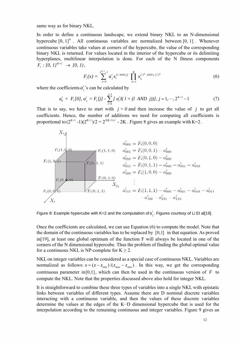
In order to define a continuous landscape, we extend binary NKL to an N-dimensional hypercube . All continuous variables are normalized between . Whenever continuous variables take values at corners of the hypercube, the value of the corresponding binary NKL is returned. For values located in the interior of the hypercube or its delimiting hyperplanes, multilinear interpolation is done. For each of the N fitness components

N[0, 1] [0, 1]

K+1iF : [0, 1] [0, 1)→ ,

1

1

k+1k

k

K2i [1 AND j] [ 2 AND j ] 2

i j i ij=0 k

F (x) = a x x−

=∑ ∏

k

1

(6)

where the coefficients ’s can be calculated by ija

11, 1, , 2

ji i i K0 i j i l

l=0a = F [0], a = F [j] - [ a I( l = (l AND j))] j

−+= −∑ L (7)

That is to say, we have to start with and then increase the value of to get all coefficients. Hence, the number of additions we need for computing all coefficients is proportional to . Figure 8 gives an example with .

j = 0 j

K+1 K+1 2(K+1)-1(2 -1)(2 )/2 = 2 - 2K K=2

Figure 8: Example hypercube with K=2 and the computation of . Figures courtesy of Li Et al[19]. ija

Once the coefficients are calculated, we can use Equation (6) to compute the model. Note that the domain of the continuous variables has to be replaced by in that equation. As proved in[19], at least one global optimum of the function F will always be located in one of the corners of the N dimensional hypercube. Thus the problem of finding the global optimal value for a continuous NKL is NP-complete for K ≥ 2.

[0,1]

NKL on integer variables can be considered as a special case of continuous NKL. Variables are normalized as follows: min max min( ) /( )x z z z z= − − . In this way, we get the corresponding continuous parameter in[0,1] , which can then be used in the continuous version of to compute the NKL. Note that the properties discussed above also hold for integer NKL.

F

It is straightforward to combine these three types of variables into a single NKL with epistatic links between variables of different types. Assume there are D nominal discrete variables interacting with a continuous variable, and then the values of these discrete variables determine the values at the edges of the K−D dimensional hypercube that is used for the interpolation according to the remaining continuous and integer variables. Figure 9 gives an

12

example. The individual has three parameters of different types and each variable interacts with both of the other two. For each variable, a hypercube is created. Assume

. The fitness value of this individual is calculated as follows. dX = 0,

iX = 0.4, rX = 0.8, L = 3

Figure 9: Sample computation of MI-NKL. The bottom left table is the epistasis matrix and table on the right the fitness matrix. Figures courtesy of Li Et al.[19].

3.3 ADG-based Mixed Integer Landscapes

A natural test problem for BOA would be a problem which can model one-way dependences between variables. Traditional mixed integer NK landscapes can deal with undirected interaction between variables and will be modified next to incorporate one-way interaction. In practice one-way dependency is more frequently encountered than the bilateral interaction as defined in classical NKL. We thus introduce ADG-based NKL. Let 1( , )NX X X= L denote a set of decision variables and assume the interaction structure of them is described by some ADG, where the nodes represent parameters to be optimized and for each node a set of parent nodes are assigned. Then the ADG-based NKL can be written as a function of component functions as equation (8). Note that this expression has similar structure with the logarithm expression of in equation (4).

iF ( )P X

1( ) ( , ( ))

N

i i ii

F x F x parents x=

= ∑ (8)

The construction of ADG-based NKL corresponds to that of classical NKL with merely one exception. Note that K can vary with the index of the decision variable in question, depending on how many parents it has. Thus the K in the expression ’ ADG-based NKL’ is not referring to the number of epistatic genes anymore, however we kept it as it makes it easier to match the corresponding well known NK-landscapes with the ADG-based NK landscapes. Take binary case as an example, the size of the fitness matrix for a classical NKL with interaction level K is while for ADG-based NKL, the fitness vector for each node can be of different size. A node with parents has the fitness vector of elements. The way to calculate fitness is the same as for general NKL. Figure 10 gives an example of an ADG-based MI-NK Landscape. Note that though we use ADG to define dependences, the formalism is actually meant to represent independences, which means all the independences that hold according to

K+1N-by-2k k+12

13

the network should also hold for the probability distribution P while the other way around does not stand. But in our construction of ADG-based NKL, we assume two nodes have parent-son dependency once an arc exists between them. It can be considered that we take an extreme interpretation of ADG here.

Figure 10: Example for an ADG-base landscape. The function values at the edge of the search space are set randomly between 0 and 1. As non-discrete nodes are involved, values in between are interpolated. Courtesy of Li.

14

Chapter 4 Experiments and Results We use Matlab7.1 for the programming and Kevin Murphy’s Bayesian Network Toolbox for MatLab: http://bnt.sourceforge.net/ for implementing Bayesian networks. The objective is to minimize.

4.1 PBIL on Standard Binary NK Landscapes

PBIL inherits the advantage of GA as well as incremental learning. As there are many parameters involved, we focus on the learning rateα which, as stated above, explicitly controls the speed of convergence of the algorithm. Furthermore, to get deeper understanding of the complexity introduced by interaction level K, we will apply PBIL on NKL over different K. To make the notation simple, we denote the epistasis matrix as E and use the seed number to represent the according binary fitness landscape.

Figure 11 plots the differences between the best fitness achieved and the global optimum versus the number of evaluations for a sample case of K = 3 and D = 15, with E = [8 13 2; 3 4 14; 14 12 15; 1 11 13; 10 13 8; 12 14 2; 6 3 11; 15 3 2; 12 15 1; 15 11 9; 4 10 9; 5 11 10; 7 3 12; 9 10 13; 5 9 1] and seed = 1000. Results are averaged over 20 runs. The population size is 28 and in each generation the probability vector is updated from the single best individual. In the figure, the blue curve decays fast within about 600 evaluations and after slightly going down further it stays flat while the red decreases gradually all through until it achieves more progress than the other around 2200 evaluations. This can be explained by the memorizing mechanics introduced by the updating rule. Larger α means less memory of the past. By always guiding the algorithm towards the best individual in current generation it speeds up the convergence surely but meanwhile it keeps losing promising solutions and as a result the searching always end in local optima. On the contrary, with smallerα PBIL searches from one to another nearby neighborhood and less likely to miss promising part of the solution space where the global optimum may exist. Therefore, α should be carefully tuned to achieve advantage of both the two as well as based on the problem in hand. However, in practice smaller α are always favored. This is out of the consideration of reliability. As can be seen from the error bar plot, the standard deviation of results from 20 runs for 0.02α = are generally smaller, especially after 2300 evaluations which means the solution we find is reliable instead of just being hit by chance. This is quite essential when dealing with practical problems. In available publications on PBIL, α is always set to 0.02 or smaller. We thus fix it as 0.02 hereafter.

Figure 11: The effect of learning rate on PBIL’s performance. The right figure plots the average differences between the best fitness achieved and the global optimum versus the number of evaluations and the left is the errorbar. Red curve is for learning rate of 0.02 and blue for 0.1.

15

Figure 12: Generation needed to converge for different K. The general trend is observed: the larger K, the more generation needed.

Figure 13: Vector field of p[s/p] for K=1 and D=2. Seed for generating landscapes are 63719 and 22079, respectively. In the first case the algorithm converges to global optimum regardless of the initialization of probability vector. For the second, it is different for different fitness matrices and initialization of probability vector decides where to converge. For p0= [0.5 0.5], all converge to global optimum.

Figure 14: left: PBIL converges to global optima [0 1 1] for seed 118399. The diamond marks the initialized probability vector and red circle the global optimum. The curve is the trajectory of the conditional mean of best individual in next generation. Right: For seed 100693, PBIL converges to local optima [0 0 1] instead of [1 1 0], the global optimum.

We then study how K affects the performance of PBIL. The searching is terminated until the difference between global fitness maximum and the best fitness found is smaller than1e-6 or the total evaluation of 5000 times has been done. Figure 12 shows the counterpart evaluation

16

needed to find the global optimum for K from 1 to 8. For each K, the evaluation is needed is averaged over 10 epistasis matrices and for every fixed epistasis matrix 10 randomly fitness matrices. Due to the limited trails carried out, it is may be not precise and we can still see the general trend of increasing as K gets larger. This matches the idea that larger K introduces more complexity.

Next we will study the theoretical aspects of the convergence behavior of PBIL. As proved in[11], the simple dynamics of PBIL’s update rule ensure convergence with probability 1 to the global optimum in the case of linear pseudo Boolean functions. As for nonlinear problems, the behavior of PBIL becomes more complex. It can be attracted by local solutions as well.

The updating rule of PBIL is: [11] ( )( 1),

1

1 ttk

Kp

λ

y µλ+

=

= ∑ (8)

( )( 1) ( ),

1

1(1 )tt t

kk

p pλ

y µα αλ

+

=

= − + ∑ (9)

Where (0) {0.5}Dp = . Whereas rule (8) is associated with gene pool combination and selection, rule (9) is especially associated with PBIL. Note that both rules lead to stochastic algorithm that can be modeled via Markov chain. With update rule (8), ( )tp can be absorbed with nonzero probability to any vector ( ) Dp ∞ ∈Β , that is, the algorithm may converge to any accessible solution. In contrast, with update rule (9), since holds for all provided that

( ) (0,1)tp ∈ D 0t ≥(0) (0,1)Dp ∈ , the process can not be trapped in points represented by DΒ .

However, it is still possible that the process converge to a corner of the hypercube. In the best case the global solution is the only point to which the process will stochastically converge. Even if the local solutions were candidates of such events, PBIL would be preferable to the EA associated with update rule (8).

In the following, we will investigate the convergence properties of PBIL via the limitation of the mean of the stochastic probability vector sequences, that is, . As common

practice, only the special case with

( )lim [ ]t

tE p

→∞

1λ = is considered. In this case, the probability vector moves toward the best individual, which leads to

( 1) ( ) ( )(1 )t t tp p sα α+ = − + (10) where is the best individual. Since is bounded, the mean and limit can be exchanged.

( )ts ( )[ tE p ]

t

]t

)]t

)

(11) ( ) ( )lim [ ] [lim ]t

t tE p E p

→∞ →∞=

To get , the conditional probability of (10) needs to be considered. ( )[lim ]t

tE p

→∞

(12) ( 1) ( ) ( ) ( ) ( )[ / ] (1 ) [ /t t t tE p p p E s pα α+ = − +Since , we get ( 1) ( ) ( 1)[ [ / ]] [ ]t t tE E p p E p+ +=

( 1) ( ) ( )[ ] (1 ) [ ] [ (t tE p E p E F pµα α+ = − + (13)

where , which is easy to be computed as: ( ) ( ) ( )[ / ] (t t tE s p F pµ=

1 10

[ / ] { }

{ } { ( ) ( )} { ( ) ( )}k kk

E s p x p s x

x p b x p f b f x p f b f xµ λ− − −=

= ⋅ =

= ⋅ = > ⋅ ≥

∑

∑ ∑ (14)

Note that the representation has been abbreviated and provided 1...( ) (0,1)Di i Dp p == = , then

17

1

1

{ } (1 )i

i

xDx

i ii

p b x p p−

=

= = −∏

( ) ( )

{ ( ) ( )} ( )Dy

f y f x

p f b f x p b y∈Β

=

= = =∑

( ) ( )

{ ( ) ( )} ( )Dy

f y f x

p f b f x p b y∈Β

>

= = =∑

To illustrate how the idea works, we consider the simplest case of 1, 2, 2K D µ= = = . Figure 13 plots sample vector fields of E[s/p] for different fitness matrices (seed). For some seeds (left), E[s/p] converges to the global optima [1 1]. Thus it is reasonable to conclude that PBIL converges to the global optima [1 1] despite of the lack of theoretical verification. In some other case (right), the convergence behavior depends on the initial value of probability vector P0. It will converge to [0 1] or get trapped into local optima [1 0] with certain probability separately. However, since in the practice, P is initialized as [0.5 0.5], the algorithm will converge to the global optimum [0 1] too. And this convergence behavior is common in all the trails we tried.

We then consider K=2 and D=3. Things get more complicated. For some seed, p[s/p] converges to global optimum (Figure 14 left). While for some other seeds like seed 100693, it converges to local optimum instead (Figure 14 right). That is to say, for NKL, the mechanics of PBIL can not ensure convergence to global optima. To tackle the problem, mutation can be introduced, expected to help escape the local optima. But unlike classical EAs, the mutation is carried out directly on the probability vector instead of individuals.

4.2 PBIL, MIES and BOA on ADG-Based NK Landscapes

In this section, we managed to compare the three algorithms that can deal with mixed-integer optimization: PBIL, MIES and BOA. Based on[20], the setting of MIES will be as follows: ( , / 7)µ µ selection strategy for the population and offspring size and

. This means an individual step size for each variable instead of a single step-size. We choose individual step size mode because the target landscape NKL can be highly rugged in which case each variable should be carefully tuned to approach the optima and a common step size in all direction may be too coarse so that the optima can be easily missed. Assume is the number of possible values for discrete variables, and

the bound of continuous and integer variables, respectively. In the experiment step sizes for continuous and integer are initialized to 0.2 of the length of corresponding range and for discrete variables strategy parameters are initialized to 0.1.

r{ (n = n , σ

zn = n , ζ p dn = n )}

L c[min , max ]c

ii[min , max ]

The PBIL is now extended to mixed-integer case. In our experiment, we will consider the basic strategy given no specific indication, namely updating the module merely based on the best individual. In this case, the standard deviation σ will keep constant. To initialize the module, the probabilities of a discrete variable taking each value are set to the same constant value. For continuous or integer variables, is set to the median of the corresponding boundary and mσ the half of the length of the boundary so that theoretically the population can cover the whole solution space. Meanwhile, we fix the learning rate at 0.02.

The implementation of BOA is quite straightforward. We use a ( , / 2)µ µ selection strategy. As for the internal parameters for Bayesian network like the threshold for terminating the learning process, this is the default value and we made no adaptation.

18

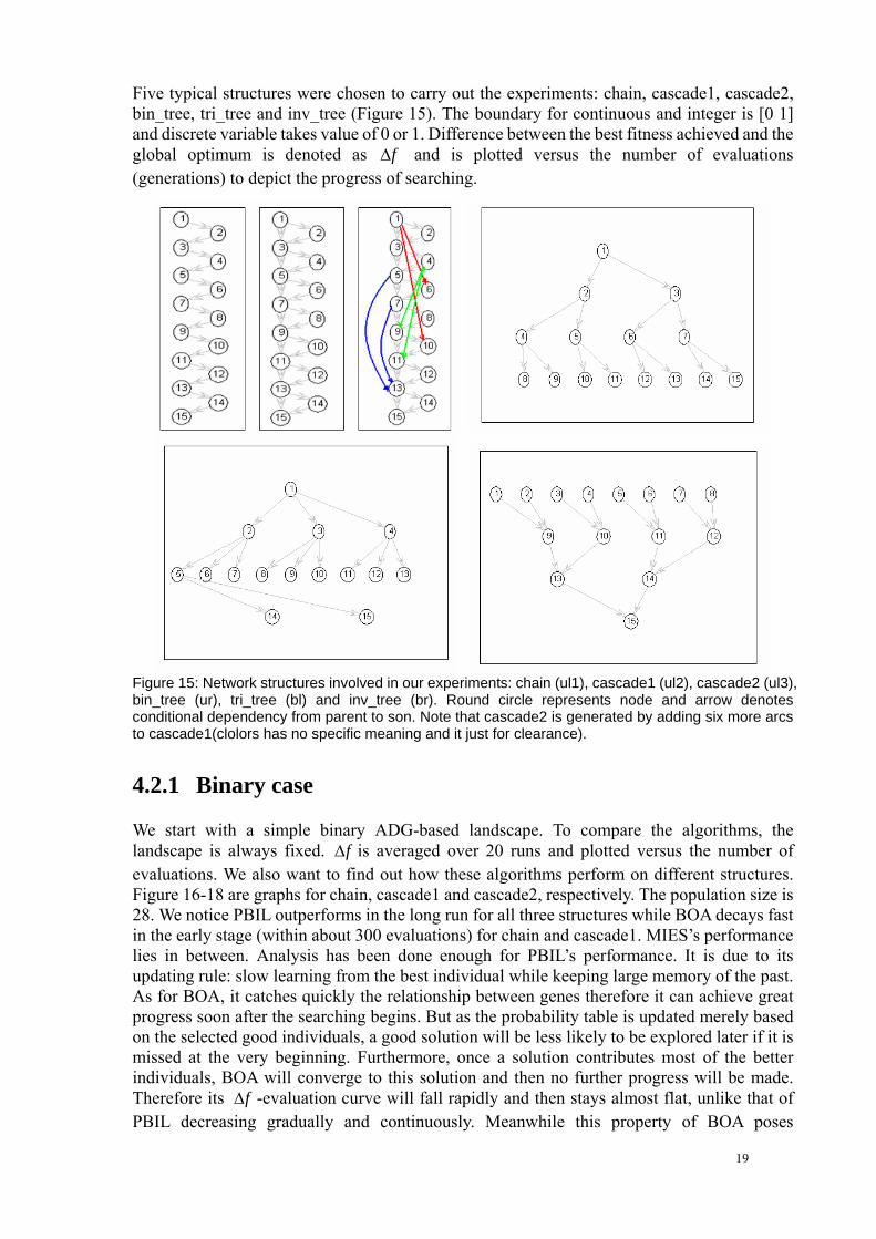
Five typical structures were chosen to carry out the experiments: chain, cascade1, cascade2, bin_tree, tri_tree and inv_tree (Figure 15). The boundary for continuous and integer is [0 1] and discrete variable takes value of 0 or 1. Difference between the best fitness achieved and the global optimum is denoted as f∆ and is plotted versus the number of evaluations (generations) to depict the progress of searching.

Figure 15: Network structures involved in our experiments: chain (ul1), cascade1 (ul2), cascade2 (ul3), bin_tree (ur), tri_tree (bl) and inv_tree (br). Round circle represents node and arrow denotes conditional dependency from parent to son. Note that cascade2 is generated by adding six more arcs to cascade1(clolors has no specific meaning and it just for clearance).

4.2.1 Binary case

We start with a simple binary ADG-based landscape. To compare the algorithms, the landscape is always fixed. is averaged over 20 runs and plotted versus the number of evaluations. We also want to find out how these algorithms perform on different structures. Figure 16-18 are graphs for chain, cascade1 and cascade2, respectively. The population size is 28. We notice PBIL outperforms in the long run for all three structures while BOA decays fast in the early stage (within about 300 evaluations) for chain and cascade1. MIES’s performance lies in between. Analysis has been done enough for PBIL’s performance. It is due to its updating rule: slow learning from the best individual while keeping large memory of the past. As for BOA, it catches quickly the relationship between genes therefore it can achieve great progress soon after the searching begins. But as the probability table is updated merely based on the selected good individuals, a good solution will be less likely to be explored later if it is missed at the very beginning. Furthermore, once a solution contributes most of the better individuals, BOA will converge to this solution and then no further progress will be made. Therefore its -evaluation curve will fall rapidly and then stays almost flat, unlike that of PBIL decreasing gradually and continuously. Meanwhile this property of BOA poses

f∆

f∆

19

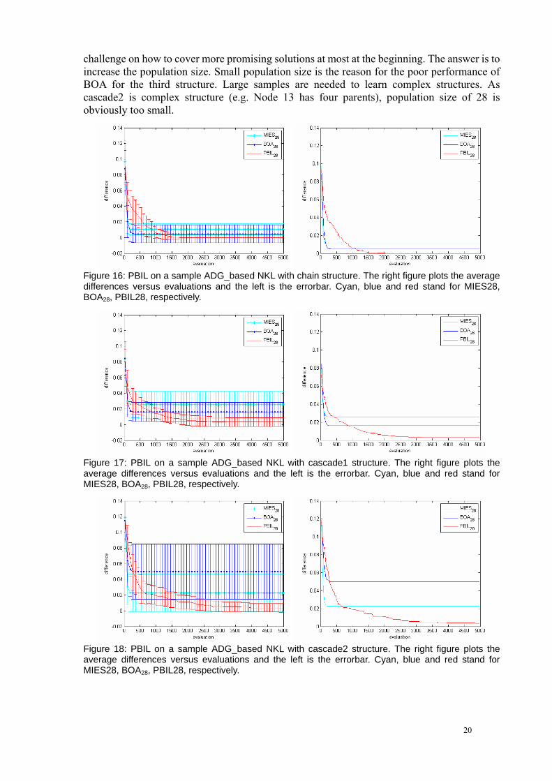
challenge on how to cover more promising solutions at most at the beginning. The answer is to increase the population size. Small population size is the reason for the poor performance of BOA for the third structure. Large samples are needed to learn complex structures. As cascade2 is complex structure (e.g. Node 13 has four parents), population size of 28 is obviously too small.

Figure 16: PBIL on a sample ADG_based NKL with chain structure. The right figure plots the average differences versus evaluations and the left is the errorbar. Cyan, blue and red stand for MIES28, BOA28, PBIL28, respectively.

Figure 17: PBIL on a sample ADG_based NKL with cascade1 structure. The right figure plots the average differences versus evaluations and the left is the errorbar. Cyan, blue and red stand for MIES28, BOA28, PBIL28, respectively.

Figure 18: PBIL on a sample ADG_based NKL with cascade2 structure. The right figure plots the average differences versus evaluations and the left is the errorbar. Cyan, blue and red stand for MIES28, BOA28, PBIL28, respectively.

20

Figure 19: The population size of BOA. Blue, cyan and red indicate BOA28, BOA80, BOA100, respectively.

Figure 20: PBIL on a sample ADG_based NKL with chain structure. The right figure plots the average differences versus evaluations and the left is the errorbar. Cyan, blue and red stand for MIES100, BOA100, PBIL100, respectively.

Figure 21: PBIL on a sample ADG_based NKL with cascade1 structure. The right figure plots the average differences versus evaluations and the left is the errorbar. Cyan, blue and red stand for MIES100, BOA100, PBIL100, respectively.

21

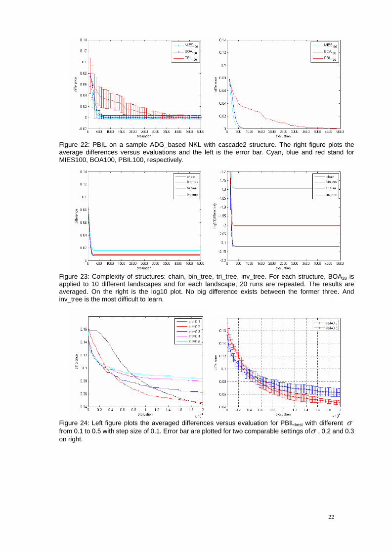
Figure 22: PBIL on a sample ADG_based NKL with cascade2 structure. The right figure plots the average differences versus evaluations and the left is the error bar. Cyan, blue and red stand for MIES100, BOA100, PBIL100, respectively.

Figure 23: Complexity of structures: chain, bin_tree, tri_tree, inv_tree. For each structure, BOA28 is applied to 10 different landscapes and for each landscape, 20 runs are repeated. The results are averaged. On the right is the log10 plot. No big difference exists between the former three. And inv_tree is the most difficult to learn.

Figure 24: Left figure plots the averaged differences versus evaluation for PBILbest with different σ from 0.1 to 0.5 with step size of 0.1. Error bar are plotted for two comparable settings ofσ , 0.2 and 0.3 on right.

22

Figure 25: Comparison of algorithms on a sample ADG_based NKL with chain structure. The right figure plots the average differences versus evaluation and the left is the error bar. Cyan, blue and red stand for MIES28, BOA28 and PBIL28, respectively.

We thus try larger population sizes. As Figure 19 shows, larger population results in slower decrease of in the early stage but smaller f∆ f∆ in the long run. For size of 100, BOA reaches the global optima after about 600 evaluations. This effect of population size introduces more flexibility into BOA application. Based on the practical problem at hand, we can choose smaller population for fast convergence but large population whenever final performance is more crucial and more evaluations are permitted. Generally, to find the balance of the two is important and too small population should be avoided noticing the change of standard deviation in the left error bar graph. The population is similar to the effect of the learning rate in PBIL.

Three algorithms with population size of 100 are then applied to the same landscapes used above. Figure 20-22 plot the results. BOA outperforms PBIL through most of the searching process. And it always finds the global optima. In the long run PBIL is comparable to BOA. MIES is also featured by fast convergence and we notice the convergence speed is less affected by the population size.

One doubt concerning the complexity of the network structure is aroused in our experiments. We get the visual impression that the complexity increased from chain to bin_tree and tri_tree. But experiments results indicate differently. For this comparison, 10 different landscapes are tried for each structure and for each landscape, 20 runs are repeated. Figure 23 plots the averaged from BOA and its log plot. The plot shows similar performances of BOA over the three structures. The results also show that the inv_tree2 is the most difficult to learn. This is partly contributed by the independency introduced by nodes on the first level. But considering the four structures all together, it is reasonable to conclude that the complexity of network structure is essentially decided by the parent-to-son dependency instead of others. There are comparable conditional dependences existing in chain and tree structures. And in inv_tree, some nodes are conditional dependent to two parents, which surely increase the complexity of the network.

f∆

4.2.2 Continuous case

We first study how the value of the constant variance affects the performance of PBIL. The landscape is fixed, generated from the chain structure. As mentioned, σ is initialized as 0.5 for all variables and then kept constant of different values from 0.1 to 0.5 with step size 0.1. The results are plotted in Figure 24. It shows the larger the constant variance, the faster it converges. Larger standard deviation performs better in the very early stage though margin is decreasing as σ increases to 0.3 and higher. However in the long run, PBIL with smaller variance can

23

get closer to the global optima within evaluations permitted. This is not surprising and can be explained in this way: with largeσ , PBIL always explores a larger neighborhood thus it can soon locate where promising solutions locate in the whole solution space but as the newly generated populations are always sparsely scattered, the search of best solution is coarse and not well manipulated or guided, generally the optima is not likely to be found. On the contrary, smaller σ tune the search deliberately. It enables PBIL to exploit the neighborhood of the current center (mean) carefully and once a more promising solution is found, PBIL moves to exploit the small neighborhood centered at it. In this way, better solutions are always less likely to be missed. However this does not mean the smaller thestd , the better the algorithm is because PBIL with smaller σ takes larger risk of getting trapped in local optima. Given above-all consideration, it is important to choose σ that can balance the converge speed of the algorithm and its long-term performance. We will exclude 0.1 because practically the number of evaluations permitted is always much smaller than 20000 and too slow progress is unacceptable. Furthermore, it is reasonable to consider that the latter three strategies are not competent compared with 0.3σ = because the convergence do not speed up much while long term performance worsen obviously. As for 0.2 and 0.3, they appear to be comparable and exactly which one to choose depends on practical problem at hand. For example, if the maximum evaluation is limited to 4000 to 5000, then 0.3 is favorable while for larger evaluation 0.2 is expected to find more promising solutions. In later experiments, the variance of continuous variables in PBIL is set to 0.2.

Figure 25 plots the averaged difference versus evaluations for three algorithms with population size 28. Compared to binary case, it seems more difficult to achieve progress. And BOA is obviously better than the other two, either in term of the fast convergence in the early stage or the performance in the long run. Due to the huge computational complexity introduced by interpolation, we did not carry out further experiments with larger population size or more complex structures. But we can image that even for BOA100, it is not likely to find the exact global optima which lies in the corner of hypercubes.

Another point we would like to mention is that there are some variants of PBIL available for continuous case (so is for discrete case). They all try to improve the algorithm by employing different selection strategy or introducing new or well-polished updating rule. PBIL2-1 is among them. It introduces an updating rule formulated as:

(15) mean = (1- LR) * mean + LR * (best_1+ best_2- worst)Where best_1, best_2, worst represent the best two and the worst individuals in current generation, respectively. So the updating rule means the center of the contribution is updated from the two best and the worst individuals in current generation. Figure 26 plots the performance of three algorithms on chain structure. The population sizes are 28 for all. It shows PBIL2-1 outperforms PBILbest all through the search. Its superiority over PBILbest is fully expected because it employs more advanced updating rule which takes three individuals instead of one, namely more information available, to guide the searching. Furthermore, it incorporates not only positive but also negative learning by pushing the searching toward the best two individuals and away from the worst. Another factor contributing to the performance of it isσ . Actually we compute σ as the standard deviation of the selected three individuals, the two best the worst, thus it is always large until the algorithm converges. Maybe that is why it outperforms BOA in the long run. It is effective dealing with continuous optimization. However, considering the difficulty of its implementation in mixed-integer case we will not exploit it further since our ultimate objective is mixed-integer optimization.

24

Figure 26: Comparison of PBIL2-1, BOA and PBILbest on a sample ADG_based NKL. The population size is 28. Black, blue and red indicates PBIL2-1, BOA and PBILbest, respectively. PBIL2-1 outperforms BOA in the long run.

4.2.3 Mixed integer case

We then managed to apply algorithms on MI-NKL. Still 15 variables are considered, 5 for each type. The implementation of algorithms has been described in Chapter 2. Parameter settings are the same as in previous experiments.

Figure 27-32 are results for six sample landscapes, each with a different structure. Two different population sizes, 28 and 100, are tried. The first impression is PBIL is less competitive than it is in binary case. It proves that best setting for uni-type case is not necessarily favorable for mixed-integer problem because variables are not independent to each other. The finding of optimal solution is more than optimizing each gene or even each type of genes independently. Moreover, the PBIL strategy employed is far from being complete. Actually PBILbest we use is the very original PBIL. Many updated selection strategies and advanced learning rules have been proposed ever since but we do not take them into our experiments. This is partly due to the consideration of difficulty of implementation. What’s more, our objective is not demolishing the algorithms but to compare the basic ideas and essential mechanisms of them.

Increasing population size has different effects on three algorithms. As MIES and BOA both are featured by fast convergence, with larger population size BOA makes much more progress in the long run but the performance of MIES does not definitely improve. Of course convergence slows down a little for BOA100. BOA100 also witness dramatic decrease of standard deviation in the error bar plot which indicates higher reliability of solution found in one trail. Note that BOA28 fails for structure cascade2. Remember more complex structure requires larger amount of individuals to learn. Actually we expect to witness better performance if increasing the population size further and better, more reliable solution can be found.

We also did some statistics on different structures. For each structure, algorithms with different sizes are applied to 20 landscapes. With each fixed landscape we do ranking on the six strategies according to after certain numbers of evaluations and the ranking are then averaged over 20 landscapes. Table 2 lists the average ranks and Table sums up the ranks for all structures.

f∆

From Table , we observe the absolute superiority of BOA and incompetence of PBIL. Two BOA strategies generally rank the top two and PBILs appear to be the bottom two, mostly ranking as the ‘5’ or ‘6’. MIESs are in between.

25

Figure 27: Comparison of algorithms on a sample ADG_based MI-NKL with chain structure. The upper row plots the average differences versus evaluations and errorbar (left) for three algorithms with population size 28. Figures on the second row are for population size of 100.

Figure 28: Comparison of algorithms on a sample ADG_based MI-NKL with bin_tree structure. The upper row plots the average differences versus evaluations and errorbar (left) for three algorithms with population size 28. Figures on the second row are for population size of 100.

26

Figure 29: Comparison of algorithms on a sample ADG_based MI-NKL with tri_tree structure. The upper row plots the average differences versus evaluations and errorbar (left) for three algorithms with population size 28. Figures on the second row are for population size of 100.

Figure 30: Comparison of algorithms on a sample ADG_based MI-NKL with inv_tree structure. The upper row plots the average differences versus evaluations and errorbar (left) for three algorithms with population size 28. Figures on the second row are for population size of 100.

27

Figure 31: Comparison of algorithms on a sample ADG_based MI-NKL with cascade1 structure. The upper row plots the average differences versus evaluations and errorbar (left) for three algorithms with population size 28. Figures on the second row are for population size of 100.

Figure 32: Comparison of algorithms on a sample ADG_based MI-NKL with cascade2 structure. The upper row plots the average differences versus evaluations and errorbar (left) for three algorithms with population size 28. Figures on the second row are for population size of 100.

28

PBIL

28

6 5 5 4 5 PBIL

28

5 5 5 3 4 PBIL

28

5 5 5 3 3

PBIL

100

5 6 6 6 4 PBIL

100

6 6 6 6 6 PBIL

100

6 6 6 6 6

MIE

S 28

2 3 3 3 2 MIE

S 28

2 3 3 4 3 MIE

S 28

2 3 4 4 2

MIE

S 100

4 4 4 5 6 MIE

S 100

4 4 4 5 5 MIE

S 100

4 4 3 5 5

BO

A28

1 1 2 2 3 BO

A28

1 1 1 2 2 BO

A28

1 2 2 2 4

Cas

cade

1

BO

A10

0

3 2 1 1 1

Tri_

tree

B

OA

100

3 2 2 1 1

Cha

in

BO

A10

0

3 1 1 1 1

PBIL

28

5 5 5 5 5 PBIL

28

5 5 5 5 6 PBIL

28

5 5 5 5 5

PBIL

100

6 6 6 6 6 PBIL

100

6 6 6 6 5 PBIL

100

6 6 6 6 6

MIE

S 28

2 3 4 4 3 MIE

S 28

2 3 3 3 3 MIE

S 28

2 1 3 3 2

MIE

S 100

4 4 1 2 2 MIE

S 100

4 4 4 4 4 MIE

S 100

4 4 4 4 4

BO

A28

1 1 3 3 4 BO

A28

1 1 2 2 2 BO

A28

1 3 2 2 3

Cas

cade

2

BO

A10

0 3 2 2 1 1

Inv_

tree

B

OA

10

0 3 2 1 1 1

Bin

_tre

e B

OA

10

0 3 2 1 1 1

Stru

ctur

e

Alg

orith

m

1000

eva

l. 20

00 e

val.

5000

eva

l. 10

000e

val

2000

0eva

l

Stru

ctur

e A

lgor

ithm

1000

eva

l. 20

00 e

val.

5000

eva

l. 10

000e

val

2000

0eva

lSt

ruct

ure

Alg

orith

m

1000

eva

l. 20

00 e

val.

5000

eva

l. 10

000e

val

2000

0eva

l

Tabl

e 2:

The

rank

ing

of P

BIL

28, P

BIL 1

00, M

IES 2

8, M

IES 1

00, B

OA 2

8, BO

A 100

ove

r diff

eren

t stru

ctur

es. T

he re

sults

ave

rage

ove

r 20

land

scap

es.

29

30

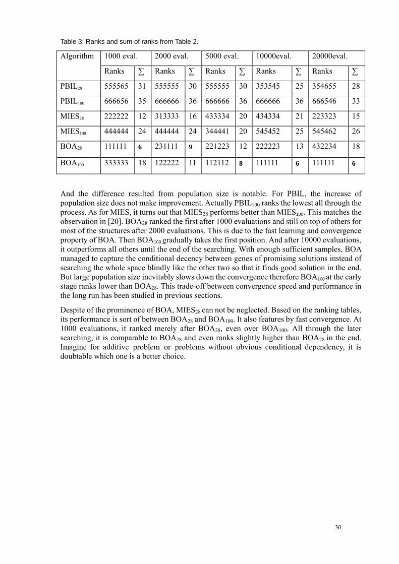
Table 3: Ranks and sum of ranks from Table 2.

1000 eval. 2000 eval. 5000 eval. 10000eval. 20000eval. Algorithm

Ranks ∑ Ranks ∑ Ranks ∑ Ranks ∑ Ranks ∑

PBIL28 555565 31 555555 30 555555 30 353545 25 354655 28

PBIL100 666656 35 666666 36 666666 36 666666 36 666546 33

MIES28 222222 12 313333 16 433334 20 434334 21 223323 15

MIES100 444444 24 444444 24 344441 20 545452 25 545462 26

BOA28 111111 6 231111 9 221223 12 222223 13 432234 18

BOA100 333333 18 122222 11 112112 8 111111 6 111111 6

And the difference resulted from population size is notable. For PBIL, the increase of population size does not make improvement. Actually PBIL100 ranks the lowest all through the process. As for MIES, it turns out that MIES28 performs better than MIES100. This matches the observation in [20]. BOA28 ranked the first after 1000 evaluations and still on top of others for most of the structures after 2000 evaluations. This is due to the fast learning and convergence property of BOA. Then BOA100 gradually takes the first position. And after 10000 evaluations, it outperforms all others until the end of the searching. With enough sufficient samples, BOA managed to capture the conditional decency between genes of promising solutions instead of searching the whole space blindly like the other two so that it finds good solution in the end. But large population size inevitably slows down the convergence therefore BOA100 at the early stage ranks lower than BOA28. This trade-off between convergence speed and performance in the long run has been studied in previous sections.

Despite of the prominence of BOA, MIES28 can not be neglected. Based on the ranking tables, its performance is sort of between BOA28 and BOA100. It also features by fast convergence. At 1000 evaluations, it ranked merely after BOA28, even over BOA100. All through the later searching, it is comparable to BOA28 and even ranks slightly higher than BOA28 in the end. Imagine for additive problem or problems without obvious conditional dependency, it is doubtable which one is a better choice.

31

Chapter 5 Summary and Outlook We work on utilizing Estimation of Distribution Algorithms to do mixed integer optimization with known structure of gene dependences. MI-PBIL and MI-BOA, together with MIES, have been applied to artificial test problem: ADG-based MI-NKL, mixed-integer NK Landscapes with gene dependences structured as ADGs. MIES and PBIL work under the assumption of gene independency so they are incapable of grasping the dependences between variables. Experiments shows BOA can capture the dependency between genes soon after the searching begins. However the population size is crucial. By manipulating it, trade-off can be made between the convergence speed and performance in the long run. Generally for more complex structures, more individuals BOA requires to learn the dependency. Furthermore, larger population size increases the reliability of the solution found thus is favored in practice. Altogether BOA is promising for practical problems which feature ADG-structured dependences between multi-type variables.

However there is still much to do in the future. In terms of algorithm development, PBIL has been extended to mixed-integer case but is still far from being complete. Actually experiments show it is much less competitive even than the well-polished MIES for mixed-integer optimization. Though theoretically it is incapable of dealing with gene interaction, just like MIES, it can be well developed for optimization problems with tight building blocks or elsewhere BOA can not work. Improvement can be made with respect to selection strategy, updating rule and parameter settings. Furthermore, we can assume different model for the continuous variables like the histogram-based model in [1]. Besides, the treatment of integer variables is still under discussion.

As of BOA, more statistics can be done on its parameter setting, especially the population size. It is meaningful to find out the ideal population size for different problem size and the relationship between the two. There are other factors affecting the complexity of the problem such as the number of possible values taken by discrete variables. To find out whether and how it affects the ideal population size and to compare it to other competitive algorithms are important for its practical use. Moreover, insight into its running time behavior is important for algorithm evaluation too. Besides, remember Bayesian learning can be done in terms of both parameters and structures. As we did not learn the structure in this work, its performance on problem without known structure is up to further study.

As BOA turns out to be effective and robust, it has limitations of itself. It is incapable of learning the dependency of discrete mode on its continuous parent(s). Therefore we have to use discretising techniques for the continuous variable, which not only results in larger conditional probability tables and slow-down of the learning process but inevitably introduces error. Meanwhile, using Gaussian distribution as an approximation of symmetrical geometric distribution for integer variables leads to bias too. If these problems can be addressed in a better way, BOA will be functional solving real-world optimization, either uni-objective or multi-objectives.

Abbreviations and symbols

Table 2: Abbreviations and symbols

Abbreviation Full name

ADG acyclic directed graph

ADG-based NKL ADG-based mixed integer NK landscapes

BOA Bayesian optimization algorithms

EDA estimation of distribution algorithm

GA evolutionary algorithms

MI-NKL mixed integer NK landscapes

MIES mixed integer evolutionary algorithm

MI-BOA mixed integer BOA

MI-PBIL mixed integer PBIL

NKL NK landscapes

Symbol Variable name

α learning rate (LR) of PBIL

L the number of possible values for discrete variables

m Mean of Gaussian distribution

σ Standard deviation of Gaussian distribution

µ population size

λ number of individuals selected

f∆ difference between best fitness found and the global minimum

K Interaction level in NKL

N Problem dimension

F(x) Fitness of genotype over NKL x

iF (x) Fitness contribution of gene i

c c[min , max ] Boundary of continuous variables

rn , z n , dn Number of continuous, integer and discrete variables, respectively

nσ ,nζ , pn

Number of strategy parameters for continuous, integer and discrete variables while rn nσ = means single step-size for continuous variables.

32

33

Acknowledgements I’d like to thank the supervisors of this project, Dr. Michael T. M. Emmerich and PhD candidate Rui Li, for detailed instructions all through the project, their valuable ideas and advices. I also thank Ildikle Flesch and Peter Lucas for their help understanding of Bayesian networks.

I greatly appreciate Mr. Bakker’s help all through my two-year study here in Leiden.

34

References [1] B. Cobb, R. Rumi and A. Salmeron. Bayesian Network Models with Discrete and

Continuous Variables, In Advances in Probabilistic Graphical Models. pp. 81-102, 2007.

[2] B. Yuan, M. Gallagher. Playing in Continuous Spaces: Some Analysis and Extension of Population-Based Incremental Learning. In Proceedings of the 2003 Congress on Evolutionary Computation, IEEE, pp. 443 - 450, IEEE Press, NY,2003.

[3] C. González, J.A. Lozano, P. Larrañaga. The convergence behavior of the PBIL algorithm: A preliminary approach. In V Kurkova, N. C. Steele, R. Neruda, and M. Karny, editors, Proceedings of the Fifth International Conference on Artificial Neural Networks and Genetic Algorithms, ICANNGA’2001.

[4] D. Koller and U. Lerner and D. Anguelov. A General Algorithm for Approximate Inference and its Application to Hybrid Bayes nets. UAI 1999, Morgan Kauffman, 302--313, 1999.

[5] E. D. Weinberger. 1996. NP completeness of Kauffman’s N-k model, a tunable rugged fitness landscape. Working Papers 96-02-003, Santa Fe Institute, Santa Fe, NM, First circulated in 1991.

[6] G. Rudolph. An Evolutionary Algorithm for Integer Programming, In Davidor et al.: Proc. PPSN III, Jerusalem, pp. 139 - 148, Springer, Berlin, 1994.

[7] I. Servet, L. Trave-Massuyes, D. Stern. “Telephone Network Traffic Overloading Diagnosis and Evolutionary Computation Techniques”. In Artificial Evolution 97, J.-K. Hao, et al. Eds., France, pp. 137-144, Springer, 1997.

[8] J. Pearl. Bayesian Networks: A Model of Self-Activated Memory for Evidential Reasoning. In Proceedings of the 7th Conference of the Cognitive Science Society, University of California, Irvine, CA, pp. 329-334, Greenwich, CT: Albex, 1985.

[9] J. S. Ide, F. G. Cozman. Random Generation of Bayesian Networks, Proceedings of the 16th Brazilian Symposium on Artificial Intelligence: Advances in Artificial Intelligence, p.366-375, Springer-Verlag London, UK, 2002.

[10] L. Altenberg. NK Fitness Landscapes. The Handbook of Evolutionary Computation, ed. T. Back, D. Fogel, Z. Michalewicz. IOP Publishing Ltd and Oxford University Press, New York, pp. B2.7:5 - B2.7:10, 1997.

[11] M. Höhfeld, G. Rudolph. Towards a Theory of Population-Based Incremental Learning. The Proceedings of the Fourth IEEE Conference on Evolutionary Computation, pp. 1 - 5. IEEE Press, 1997.

[12] M. T. M. Emmerich, M. Schuetz, B. Gross, M. Groetzner. Mixed-Integer Evolution Strategy for Chemical Plant Optimization. In I. C. Parmee, editor, Evolutionary Design and Manufacture (ACDM 2000), pp. 55 - 67, Springer NY, 2000.

[13] M. Pelikan, D.E. Goldberg, E. Cantu-Paz. BOA: the Bayesian optimization algorithm. in Proceedings of the Genetic and Evolutionary Computation Conference GECCO-99, Orlando, Florida USA, W. Banzhaf, J. Daida, A.E. Eiben, M.H. Garzon, V. Honavar, M. Jakiela, and R.E. Smith (Eds.), vol. I, pp. 525 - 532, 1999.

[14] M. Pelikan, D.E. Goldberg, F. Lobo. “A Survey of Optimization by Building and Using Probabilistic Models”, Tech. Report No.99018, University of Illinois at Urbana-Champaign, 1999.

35

[15] M. Sebag, A. Ducoulombier, Extending Population-Based Incremental Learning to Continuous Search Spaces, Proceedings of the 5 International Conference on Parallel Problem Solving from Nature, ISBN:3-540-65078-4, pp. 418 - 427, September 27-30,

th

Springer-Verlag London, UK, 1998 .

[16] P. A. N. Bosman and D. Thierens. Expanding from discrete to continuous estimation of distribution algorithms: the IDEA. In M. Schoenauer, K. Deb, G. Rudolph, X. Yao, E. Lutton, J.J. Merelo, and H.P. Schwefeo, editors, Parallel Problem Solving from Nature, PPSN VI pp. 767 - 76, Springer, 2000.

[17] P. Larrañaga, J.A. Lozano, Eds. Estimation of Distribution Algorithms: A New Tool for Evolutionary Computation, Kluwer Academic Publishers, 2001.

[18] R. G. Cowell and A. P. Dawid and S. L. Lauritzen and D. J. Spiegelhalter. Probabilistic Networks and Expert Systems Springer-Verlag New York, ISBN 0-387-98767-3, 1999.

[19] R. Li, M.T.M. Emmerich, J. Eggermont, E. G. P. BoveNKamp, T. Bäck, J Dijkstra, J. H. C. Reiber. Mixed-Integer NK Landscape. T.P. Runarsson et al. (Eds.): PPSN IX, LNCS 4193, pp. 42 - 51. Springer-Verlag Berlin, Heidelberg, 2006.

[20] R. Li, M.T.M. Emmerich, J. Eggermont, E.G. P. BoveNKamp. Mixed-Integer optimization of Coronary Vessel Image Analysis using Evolution Strategies. in Proceedings of the Genetic and Evolutionary Computation Conference GECCO’06, Seattle, Washington, USA, pp. 1645 - 1652, 2006.

[21] R. K. Thompson, A.J. Wright. 1996. Additively decomposable fitness functions, 1996.

[22] S. A. Kauffman. Adaptation on rugged fitness landscapes. In D. Stein, editor, Lectures in the Sciences of Complexity, pp. 527 - 618. Addison-Wesley, Redwood City. SFI Studies in the Sciences of Complexity, Lecture Volume I, 1989.

[23] S. Baluja, R. Caruana. Removing the Genetics from the Standard Genetic Algorithm. The Proceedings of the 12th Annual Conference on Machine Learning, pp. 38 - 46, Carnegie Mellon University Pittsburgh, PA, USA, 1995.

[24] S. L. Lauritzen. Graphical models. Clarendon Press, Oxford, 1996.

[25] S. N. Evansi, D. Steinsaltz. Estimating some features of NK fitness landscapes. The Annals of Applied Probability, Vol. 12, No. 4, pp.1299 - 1321, 2002.