bayesian models for multiple local sequence alignment...

Bayesian Models for Multiple Local Sequence Alignment and Gibbs Sampling StrategiesAuthor(s): Jun S. Liu, Andrew F. Neuwald and Charles E. LawrenceSource: Journal of the American Statistical Association, Vol. 90, No. 432 (Dec., 1995), pp. 1156-1170Published by: American Statistical AssociationStable URL: http://www.jstor.org/stable/2291508 .

Accessed: 26/09/2014 10:55

Your use of the JSTOR archive indicates your acceptance of the Terms & Conditions of Use, available at .http://www.jstor.org/page/info/about/policies/terms.jsp

.JSTOR is a not-for-profit service that helps scholars, researchers, and students discover, use, and build upon a wide range ofcontent in a trusted digital archive. We use information technology and tools to increase productivity and facilitate new formsof scholarship. For more information about JSTOR, please contact [email protected].

.

American Statistical Association is collaborating with JSTOR to digitize, preserve and extend access to Journalof the American Statistical Association.

http://www.jstor.org

This content downloaded from 128.252.234.200 on Fri, 26 Sep 2014 10:55:06 AMAll use subject to JSTOR Terms and Conditions

http://www.jstor.org/action/showPublisher?publisherCode=astata

http://www.jstor.org/stable/2291508?origin=JSTOR-pdf

http://www.jstor.org/page/info/about/policies/terms.jsp


Bayesian Models for Multiple Local Sequence Alignment and Gibbs Sampling Strategies

Jun S. Liu, Andrew F. NEUWALD, and Charles E. LAWRENCE

A wealth of data concerning life's basic molecules, proteins and nucleic acids, has emerged from the biotechnology revolution. The human genome project has accelerated the growth of these data. Multiple observations of homologous protein or nucleic acid sequences from different organisms are often available. But because mutations and sequence errors misalign these data, multiple sequence alignment has become an essential and valuable tool for understanding structures and functions of these molecules. A recently developed Gibbs sampling algorithm has been applied with substantial advantage in this setting. In this article we develop a full Bayesian foundation for this algorithm and present extensions that permit relaxation of two important restrictions. We also present a rank test for the assessment of the significance of multiple sequence alignment. As an example, we study the set of dinucleotide binding proteins and predict binding segments for dozens of its members.

KEY WORDS: Bernoulli sampling; Dinucleotide binding; Dirichlet distribution; Fragmentation; Gibbs sampling; Metropolis algorithm; Product Multinomial; Ranks test.

1. INTRODUCTION

1 .1 Background

The linear biopolymers-DNA, RNA, and proteins-are the three central molecular building blocks of life. DNA is an information storage molecule. RNA has a wide va- riety of roles, including a small but important set of functions. Because RNA can play so many roles, it is believed to be the molecule from which life began. Proteins are the action molecules of life, responsible for nearly all of the functions of all living beings and forming many of life's structures. The diversity of functions performed by proteins is extraordinarily broad. Although the methods we describe here have been successfully applied to all the three biopolymers, to date they have been most widely used for the characterization of proteins, the focus of the application described here.

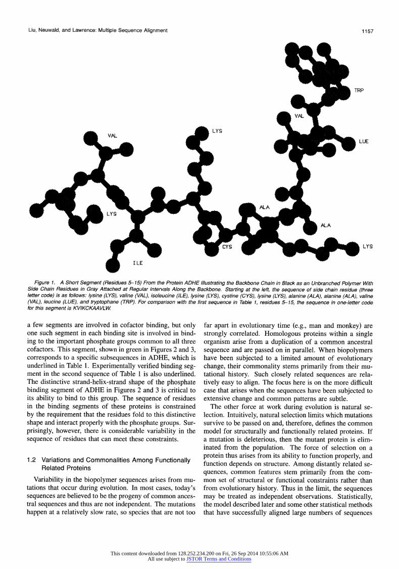
A protein is an unbranched, linear, heterogeneous polymer composed of a sequence of 20 types of amino acids. An amino acid is composed of a peptide and a side chain residue. The peptide is identical in all but one of the amino acids, proline; however, all 20 side chain residues are unique. As shown in Figure 1, the peptides link together to form the peptide backbone chain, with the side chain residues attached at regular intervals. Thus a protein may be specified in a one-dimensional representation by giving the sequence of its residues. Table 1 gives the sequence of the first four of the 91 proteins in our example.

Most proteins fold to a unique densely packed three- dimensional shape. Because of the dense packing, a figure

Jun S. Liu is Assistant Professor, Department of Statistics, Stanford Uni- versity, Stanford, CA 94305. Andrew F. Neuwald is Postdoctoral Fellow, National Center for Biotechnology Information, NLM-NIH, Bethesda, MD 20894. Charles E. Lawrence is Chief, Biometrics Lab, Wadsworth Center for Laboratories and Research, NYS-DOH, Albany, NY 12201, and a visiting Senior Scientist, National Center for Biotechnology Infor- mation, NLM-NIH. Part of the manuscript was prepared when the first au- thor was Assistant Professor, Department of Statistics, Harvard University. This work was partially supported by National Institute of Health Grant ROI HG01257-01, National Science Foundation Grants DMS-9404344 and DMS9501570, and the William F. Milton Fund. The authors thank the editor, the associate editor, and two referees for numerous constructive comments that helped improve the article.

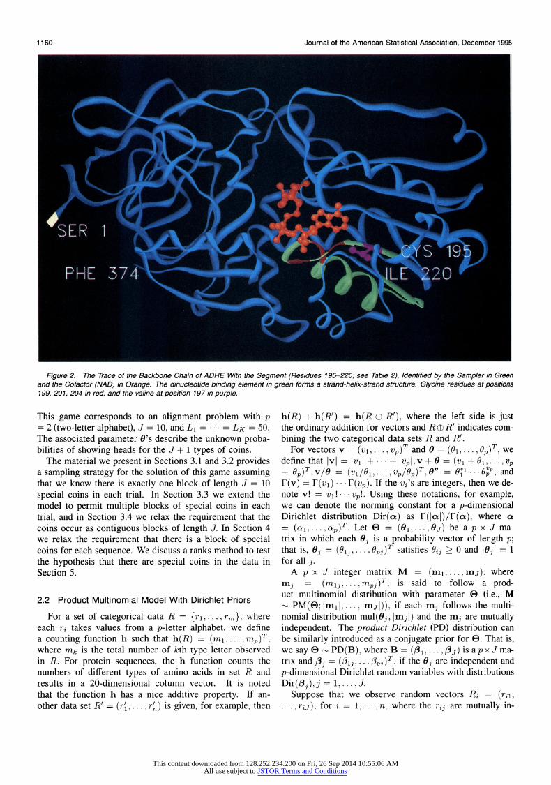
that includes all the atoms in a protein is extremely clut- tered. In Figure 2 we present only the trace of the backbone chain to illustrate the three-dimensional fold of the first protein in Table 1: horse alcohol dehydrogenase (ADHE).

Probably the most important and impressive job performed by proteins is the catalysis of biochemical reactions. Enzymes, which are complexes of one or more proteins, are extremely efficient catalysts, with efficiencies several orders of magnitude greater than the best chemical catalysts. The fact that chains of 20 simple molecules can carry out such a broad spectrum of catalytic function so efficiently makes them arguably the most impressive system in all of the natural world. In large part enzymes owe their impressive catalytic efficiency to the exacting three-dimensional structures to which they spontaneously fold.

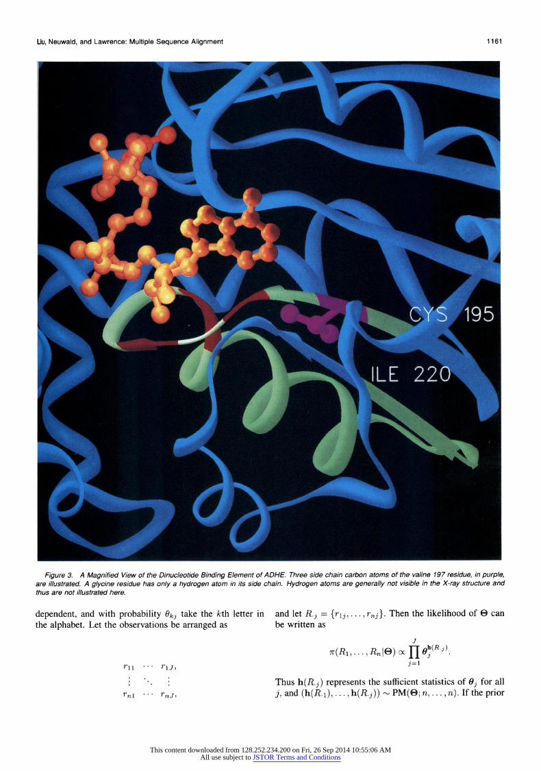
Enzymes often recruit other molecules, called cofactors, to assist in their catalytic action and perform their catalytic function through the precise interaction of the enzyme and perhaps a cofactor with the molecule to be chemically trans- formed, its substrate. This interaction requires the enzyme to bind both the substrate and the cofactor. Many cofactors are derivatives of vitamins and typically contain several chemical groups. In the example used here, three cofactors are involved: nicotinamide adenine dinucleotide (NAD), nicotinamide adenine dinucleotide phosphate (NADP), and flavin adenine dinucleotide (FAD), which are derived from niacin, niacin, and riboflavin. All three cofactors contain two phosphate groups, composed of a phosphorous atom and four oxygen atoms. In the example we focus on the binding of the enzyme to the phosphate groups in these cofactors. In Figure 2 the bound cofactor, NAD, is shown in orange. A magnified view in the vicinity of NAD is shown in Figure 3.

The critical interactions between an enzyme and a substrate, cofactor, or other bond molecule involve only a limited subset of its residues. These critical residues occur in a few segments of the protein chain. In the example,

? 1995 American Statistical Association Journal of the American Statistical Association

December 1995, Vol. 90, No. 432, Applications & Case Studies

1156



Liu, Neuwald, and Lawrence: Multiple Sequence Alignment 1157

TRP

LYS ~ ~ ~ ~ ~ ~ ~ ~ ~ ~ ~ Y

FigureV1.AALShort Segment (Residues 5-15) From the Protein ADHE Illustrating the Backbone Chain in Black as an Unbranched Polymer With

w_t~~~~~U

ILE~~_ E

Side Chain Residues in Gray Attached at Regular Intervals Along the Backbone. Starting at the left, the sequence of side chain residue (three letter code) is as follows: lysine (LYS), valine (VAL), isoleucine (ILE), lysine (LYS), cystine (CYS), lysine (LYS), alanine (ALA), alanine (ALA), valine (VAL), leucine (LUE), and tryptophane (TRP). For comparison with the first sequence in Table 1, residues 5-15, the sequence in one-letter code for this segment is KVIKCKAAVLW

a few segments are involved in cofactor binding, but only one such segment in each binding site is involved in binding to the important phosphate groups common to all three cofactors. This segment, shown in green in Figures 2 and 3, corresponds to a specific subsequences in ADHE, which is underlined in Table 1. Experimentally verified binding segment in the second sequence of Table 1 is also underlined. The distinctive strand-helix-strand shape of the phosphate binding segment of ADHE in Figures 2 and 3 is critical to its ability to bind to this group. The sequence of residues in the binding segments of these proteins is constrained by the requirement that the residues fold to this distinctive shape and interact properly with the phosphate groups. Sur- prisingly, however, there is considerable variability in the sequence of residues that can meet these constraints.

1.2 Variations and Commonalities Among Functionally Related Proteins

Variability in the biopolymer sequences arises from mutations that occur during evolution. In most cases, today's sequences are believed to be the progeny of common ancestral sequences and thus are not independent. The mutations happen at a relatively slow rate, so species that are not too

far apart in evolutionary time (e.g., man and monkey) are strongly correlated. Homologous proteins within a single organism arise from a duplication of a common ancestral sequence and are passed on in parallel. When biopolymers have been subjected to a limited amount of evolutionary change, their commonality stems primarily from their mutational history. Such closely related sequences are relatively easy to align. The focus here is on the more difficult case that arises when the sequences have been subjected to extensive change and common patterns are subtle.

The other force at work during evolution is natural selection. Intuitively, natural selection limits which mutations survive to be passed on and, therefore, defines the common model for structurally and functionally related proteins. If a mutation is deleterious, then the mutant protein is elim- inated from the population. The force of selection on a protein thus arises from its ability to function properly, and function depends on structure. Among distantly related sequences, common features stem primarily from the common set of structural or functional constraints rather than from evolutionary history. Thus in the limit, the sequences may be treated as independent observations. Statistically, the model described later and some other statistical methods that have successfully aligned large numbers of sequences



1158 Journal of the American Statistical Association, December 1995

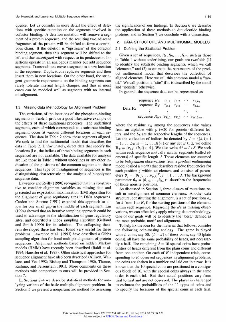
Table 1. Selected Sequences of Proteins Involved in Binding of NAD, NADP, or FAD

ADHE_HORSE: Alcohol_Dehydrogenase E Chain (EC 1.1.1.1). 2ohx

STAGKVIKCKAAVLWEEKKPFSIEEVEVAPPKAHEVRIKMVATGICRSDDHVVSGTLVTP LPVIAGHEAAGIVESIGEGVTTVRPGDKVIPLFTPQCGKCRVCKHPEGNFCLKNDLSMPR GTMQDGTSRFTCRGKPIHHFLGTSTFSQYTVVDEISVAKIDAASPLEKVCLIGCGFSTGY GSAVKVAKVTQGSTCAVFGLGGVGLSVIMGCKAAGAARIIGVDINKDKFAKAKEVGATEC VNPQDYKKPIQEVLTEMSNGGVDFSFEVIGRLDTMVTALSCCQEAYGVSVIVGVPPDSQN LSMNPMLLLSGRTWKGAIFGGFKSKDSVPKLVADFMAKKFALDPLITHVLPFEKINEGFD LLRSGESIRTILTF

LDHM_SQUAC: L-Lactate Dehydrogenase M Chain (EC 1.1.1.27) 1 dh

ATLKDKLIGHLATSQEPRSYNKITVVGVGAVGMACAISILMKDLADEVALVDVMEDKLKG EMMDLQHGSLFLHTAKIVSGKDYSVSAGSKLVVITAGARQQEGESRLNLVQRNVNIFKFI IPNIVKHSPDCIILVVSNPVDVLTYVAWKLSGLPMHRIIGSGCNLDSARFRYLMGERLGV HSCSCHGWVIGEHGDSVPSVWSGMNVASIKLHPELGTNKDKQDWKKLHKDVVDSAYEVIK LKGYTSWAIGLSVADLAETIMKNLCRVHPVSTMVKDFYGIKDNVFLSLPCVLNDHGISNI VKMKLKPDEEQQLQKSATTLWDIQKDLKF

LEU3_LEPIN: 3-Isopropylmalate Dehydrogenase (EC 1.1.1.85)

MKNVAVLSGDGIGPEVMEIAISVLKKALGAKVSEFQFKEGFVGGIAIDKTGHPLPPETLK LCEESSAILFGSVGGPKWETLPPEKQPERGALLPLRKHFDLFANLRPAIIYPELKNASPV RSDIIGNGLDILILRELTGGIYFGQPKGREGSGQEEFAYDTMKYSRREIERIAKVAFQAA RKRNNKVTSIDKANVLTTSVFWKEVVIELHKKEFSDVQLNHLYVDNAAMQLIVNPKQFDV VLCENMFGDILSDEASIITGSIGMLPSASLSESGFGLYEPSGGSAPDIAGKGVANPIAQV LSAALMLRYSFSMEEEANKIETAVRKTIASGKRTRDIAEVGSTIVGTKEIGQLIESFL

3BHS_BOVIN: 3-Beta Hydroxy-5-Ene Steroid Dehydrogenase

AGWSCLVTGGGGFLGORIICLLVEEKDLQEIRVLDKVFRPEVREEFSKLQSKIKLTLLEG DILDEQCLKGACQGTSVVIHTASVIDVRNAVPRETIMNVNVKGTQLLLEACVQASVPVFI HTSTIEVAGPNSYREIIQDGREEEHHESAWSSPYPYSKKLAEKAVLGANGWALKNGGTLY TCALRPMYIYGEGSPFLSAYMHGALNNNGILTNHCKFSRVNPVYVGNVAWAHILALRALR DPKKVPNIQGQFYYISDDTPHQSYDDLNYTLSKEWGFCLDSRMSLPISLQYWLAFLLEIV SFLLSPIYKYNPCFNRHLVTLSNSVFTFSYKKAQRDLGYEPLYTWEEAKQKTKEWIGSLV KQHKETLKTKIH

NOTE: This table shows the first 4 of the 91 sequences presented by Neuwald and Green (1994). In the first two sequences, dinucleotide-binding sites (underlined) have been experimentally determined and are also correctly predicted by the sampler. Reliable information on binding of cofactor is unavailable for the third and fourth sequences. No element is predicted by the sampler in the third sequence, and one is predicted in the forth sequence (underlined). The full data set is available at anonymous ftp site NCBI.NLM.NIH.GOV, directory pub/gibbs.

(Baldi, Chauvin, McClure, and Hunkapiller 1994; Haussler, Krogh, Mian, and Sjolander 1993) assume that sequences under analysis are independent given the common model. In many cases this assumption can be very closely achieved through careful selection of the data set. In practice we have found that the methods we propose here often work well even with substantial departures from this assumption.

There are four classes of mutations: point mutations, insertions/deletions, transpositions, and duplications. A point mutation occurs when a residue at a given point in a sequence is mutated to a new residue type. In our example we focus on proteins that bind either NAD, NADP, or FAD as a cofactor. To achieve binding there must be a force based on the energetic requirement of the protein to hold the cofactor in place. This requirement imposes constraints on point mutations in the binding site. The relationship between energetic constraints and frequencies forms the basis of statistical mechanics, pioneered by Gibbs and Boltzmann. There is an analogous relationship for residue frequencies subject to random point mutations (Berg and von Hipple 1987; Bryant and Lawrence 1991; Pohl 1971), which forms the foundation of the models used here. From

a statistical modeling perspective, this relationship is extremely valuable, because it permits us to translate from the language of physics and chemistry that governs molecular behavior to the language of statistics.

Multinomial models have been used successfully to cap- ture the variability and the limitations imposed on these sequences. Because the most important interactions of residues in a binding site area with the cofactor, substrate, or the environment rather than with one another (Bryant and Lawrence 1993), motif models that assume independence of the positions provide a good first approximation. Thus we use product multinomial models to describe the binding sites. The remainder of the enzyme forms a scaf- fold that supports the substrate binding site. Because in distantly related proteins these scaffolds can vary greatly, there is often little in common in the remainder of the protein of interest to us. Consequently, they can usually be described by a simple iid or low-order Markov sequence model.

The other three classes of mutations-insertions/deletions, transpositions, and duplications-result in changes in the length of the sequence or in reordering of the se-




quence. Let us consider in more detail the effect of deletions with specific attention on the segments involved in cofactor binding. A deletion mutation will remove a segment of a protein sequence, and the resulting two adjacent fragments of the protein will be shifted to form a contin- uous chain. If the deletion is "upstream" of the cofactor binding segment, then this segment will be shifted to the left and thus misaligned with respect to its predecessor. In- sertions operate in an analogous manner but add sequence segments. Transpositions move a segment to a new location in the sequence. Duplications replicate segments and then insert them in new locations. On the other hand, the strin- gent geometric requirements on the binding segments can rarely tolerate internal length changes, and thus in most cases can be modeled well as segments with no internal misalignment.

1.3 Missing-data Methodology for Alignment Problem

The variations of the locations of the phosphate-binding segments in Table 1 provide a good illustrative example of the effects of these mutational processes. The underlined segments, each of which corresponds to a substrate binding segment, occur at various different locations in each sequence. The data in Table 2 show these segments aligned. We seek to find the multinomial model that describes the data in Table 2. Unfortunately, direct data that specify the locations (i.e., the indices of these binding segments in each sequence) are not available. The data available for analysis are like those in Table 1 without underlines or any other in- dication of the positions of the common segments in these sequences. This type of misalignment of sequences is the distinguishing characteristic in the analysis of biopolymer sequence data.

Lawrence and Reilly (1990) recognized that it is constructive to consider alignment variables as missing data and presented an expectation maximization (EM) algorithm for the alignment of gene regulatory sites in DNA sequences. Cardon and Stormo (1991) extended this approach to al- low for one small gap in the middle of each segment. Liu (1994) showed that an iterative sampling approach could be used to advantage in the identification of gene regulatory sites, and described a Gibbs sampling algorithm (Gelfand and Smith 1990) for its solution. The collapsing theorem developed there has been found very useful for these problems. Lawrence et al. (1993) have described a Gibbs sampling algorithm for local multiple alignment of protein sequences. Alignment methods based on hidden Markov models (HMM) have recently been described (Baldi et al. 1994; Haussler et al. 1993). Other statistical approaches for sequence alignment have also been described (Allison, Wal- lace, and Yee 1992; Bishop and Thompson 1986, Thorne, Kishino, and Felsenstein 1991). More comments on these methods with comparison to ours will be provided in Sec- tion 7.

In Sections 2-4 we describe statistical methods for ana- lyzing variants of the basic multiple alignment problem. In Section 5 we present a nonparametric method for assessing

the significance of our findings. In Section 6 we describe the application of these methods to dinucleotide binding proteins, and in Section 7 we conclude with a discussion.

2. DATA STRUCTURE AND MULTINOMIAL MODELS

2.1 Defining the Statistical Problem

Given a set of sequences, R1, R2, ... , RK, such as those in Table 1 without underlining, our goals are twofold: (1) to identify the substrate binding segments, which we call "elements," and (2) to estimate the parameters of the product multinomial model that describes the collection of aligned elements. Here we call this common model a "motif." We call position a "site" if it is described by the motif and "nonsite" otherwise.

In general, the sequence data can be represented as

sequence R1: ri11 rl,2 .rl,Ll sequence R2: r2,1 r2,2 . r2,L2

Data R:

sequence RK: rK,l rK,2 ... rK,LK,

where the residue rkl among the sequences take values from an alphabet with p (=20 for protein) different let- ters, and the Lk are the respective lengths of the sequences. Let the collection of indices be denoted by I = {(k, 1): 1 = 1, ... ,LK; k = 1, ... I,K}. For any set S C I, we define Rs = {rk,l: (k, 1) C S}. We also write SC = I \ S. We seek within each sequence mutually similar segments (called elements) of specific length J. These elements are assumed to be independent observations from a product-multinomial model (called a motif) that describes residue frequencies for each position j within an element and consists of parameters Oj = (01,j,... 0pj)TIj = 1,.. ., J. The background parameter 00 = (01,0, ... I . p,o)T describes the frequencies of those nonsite positions.

As discussed in Section 1, three classes of mutations result in misalignment of common elements. Another data structure, constituting the alignment, is a set of positions ak

for k from 1 to K, for the starting positions of the elements within each sequence. Regarding the a's as missing observations, we can effectively apply missing-data methodology. One of our goals will be to identify the "best," defined as the most probable, motif and alignment.

To help fix the idea for the material that follows, consider the following coin-tossing analogy. The game is played with L coins, say 50. (L - J) of these coins, say 40 (plain coins), all have the same probability of heads, not necessar- ily a half. The remaining J = 10 special coins have probabilities of heads different from the plain coins and different from one another. On each of K independent trials, corresponding to K observed sequences in alignment problems, the coins are shaken in a tumbler and laid out in a row. It is known that the 10 special coins are positioned in a contiguous block of 10, with the special coins always in the same order is each trial. But their actual positions vary from trial to trial and are not observed. The player is challenged to estimate the probabilities of the 11 types of coins and to specify the locations of the special coins in each trial.




Figure 2. The Trace of the Backbone Chain of ADHE With the Segment (Residues 195-220; see Table 2), Identified by the Sampler in Green and the Cofactor (NAD) in Orange. The dinucleotide binding element in green forms a strand-helix-strand structure. Glycine residues at positions 199, 201, 204 in red, and the valine at position 197 in purple.

This game corresponds to an alignment problem with p = 2 (two-letter alphabet), J = 10, and L1 = = LK = 50. The associated parameter O's describe the unknown probabilities of showing heads for the J + 1 types of coins.

The material we present in Sections 3.1 and 3.2 provides a sampling strategy for the solution of this game assuming that we know there is exactly one block of length J = 10 special coins in each trial. In Section 3.3 we extend the model to permit multiple blocks of special coins in each trial, and in Section 3.4 we relax the requirement that the coins occur as contiguous blocks of length J. In Section 4 we relax the requirement that there is a block of special coins for each sequence. We discuss a ranks method to test the hypothesis that there are special coins in the data in Section 5.

2.2 Product Multinomial Model With Dirichlet Priors

For a set of categorical data Rf {rir... , where each ri takes values from a p-letter alphabet, we define a counting function h such that h(R) = (ml,mn)1.

where mk is the total number of kth type letter observed in R. For protein sequences, the h function counts the numbers of different types of amino acids in set R and results in a 20-dimensional column vector. It is noted that the function h has a nice additive property. If another data set R' = (r,.... r' ) is given, for example, then

h(R) + h(R') = h(R e3 R'), where the left side is just the ordinary addition for vectors and R e R' indicates com- bining the two categorical data sets R and R'.

For vectors v = (v, .. . , vp) and 6 = (01, ... 0 2p)T, we define that IvI = Iv1 + + Ivp ,v + 0 = (vi + 0i, . ..,vp ? 0 , )Tv/0 = (v1/01,..., vP/0P)T 9? = ovj ...QVP and r(v) = F(v1) ... F (vp). If the vi's are integers, then we denote v! = vl! v.p!. Using these notations, for example, we can denote the norming constant for a p-dimensional Dirichlet distribution Dir(a) as 1( a )/F(a) where a = (cal...coip)T. Let E = (Oi,. .. ,Oj) be a p x J matrix in which each Oj is a probability vector of length p; that is, Oj = (01j.... OSP)T satisfies i? > O and 1jIl = 1 for all j.

A p x J integer matrix M = (Ml,... ,Mj), where mj = (Mln,.. ,mpj)T. is said to follow a product multinomial distribution with parameter E (i.e., M

PM(e; m,. mj )), if each m3 follows the multinomial distribution mul(0j, in3 ) and the mj are mutually independent. The product Dirichlet (PD) distribution can be similarly introduced as a conjugate prior for e. That is, we saye - PD(B), where B = ( ,1 ... . j) is a p x J matrix and ,j = (/31j,.. . /j )T, if the Oj are independent and p-dimensional Dirichlet random variables with distributions Dir(3),j= 1,...,J.

Suppose that we observe random vectors Ri = (ni, ...,rij), for i = 1i...,n, where the ri are mutually in-




S

Figure 3. A Magnified View of the Dinucleotide Binding Element of ADHE. Three side chain carbon atoms of the valine 197 residue, in purple, are illustrated. A glycine residue has only a hydrogen atom in its side chain. Hydrogen atoms are generally not visible in the X-ray structure and thus are not illustrated here.

dependent, and with probability Okj take the kth letter in the alphabet. Let the observations be arranged as

...l n rj,

.rn 1 * rnJ,

and let R.j = {rlj,... , rn}. Then the likelihood of e can be written as

J

,T(R, *I*.*, Rn |8) aX Oh(R.j S j=1

Thus h(R.j) represents the sufficient statistics of Oj for all j, and (h(R.1), . .. , h(R.j)) -v PM(e; n, . . . , n). If the prior




distribution for E is PD(B), then the posterior distribution of e is PD(B + H), where H = (h(R.), ... . h(R.j)), The predictive distribution for the next observation Rnew or, equivalently, (h(rnew,i),. . . , h(rne,,J)) is PM(e; 1,... ,1),

where e oc (B + H) is the posterior mean of e.

3. MULTINOMIAL SAMPLING: ALIGNMENT WHEN THE NUMBER OF ELEMENTS IS GIVEN

In Sections 3.1 and 3.2 we describe a sampling-based alignment procedure when there is known to be one element in each sequence from a single motif. In Section 3.3 we generalize this to the case of multiple elements and multiple motifs. In Section 3.4 we use a fragmentation model to relax the requirement that an element has to be a contiguous block.

3.1 Model and Posterior Distributions for One Element Per Sequence

Let the starting position of the element in the kth sequence be denoted as ak, where k = 1, . . . , K, and ak can take values from 1 to Lk - J + 1. Let A = {(1,aj),..., (K,aK)}, which is the unobserved alignment. We define {A} = {(k, ak + j - 1): k = I, ... Kj = 1, ... , J}, which is the set of indices occupied by the elements with starting positions indicated in A. Let R{A} denote the collection of the residues in {A}; that is, R{A} = {rk,ak+j1l: for j = 1, ..., J; k = 1,.. ., K}. We further use {ak } to denote the set of indices occupied by the element in the kth sequence, (i.e., {ak} {(k, ak +j -1), for j 1, , J} is a collection of J consecutive positions in the kth sequence and use A(j) to denote the set of the jth positions of all elements (i.e., A(j) {(k, ak + j - 1), for

We assume that all residues outside the motif region are independently drawn from a common multinomial model characterized by a vector 0o = (01,0,... ,I Q,o)T, where I oI = 1 and 0i,0 > 0, for all i. But the residue frequencies for the motifs are modeled by PM(o) defined in Section 2, where e = (01, . .. I, Oj). Therefore, J + 1 p-dimensional parameter vectors are required to fully describe the data.

Treating the alignment data A as missing, we can write the complete-data likelihood of the parameters as

wF(R, A 0O, 0) ?' 0 h(R{A}c) 71 oh(RA(3)) (1) j=1

As was noted by Tanner and Wong (1987), this simple form of the complete-data likelihood (posterior distribution) is the key to carrying out their data augmentation algorithm. We can further use the collapsing technique of Liu (1994) to integrate out the parameter vectors 00 and e to obtain a predictive update version of the Gibbs sampler. Consequently, the resulting program, by skipping the step of drawing from product Dirichlet distributions, only involves sampling from a product multinomial distribution iteratively (whereas a standard Gibbs sampler would neces-

sarily include the step of sampling from product Dirichlet distributions).

The use of iterative sampling for Bayesian missing-data problems was first undertaken by Tanner and Wong (1987) and Li (1988). This sampling approach and its extensions have recently become a topic of great interest in Bayesian statistics. Gelfand and Smith (1990) illustrated its connec- tion with a more general method-the Gibbs sampler-and greatly popularized the idea. Some theoretical guidances, such as judging convergence and choosing efficient sam- plers, have been obtained (Gelman and Rubin 1992 and its companion discussions; Liu, Wong, and Kong 1994, 1995; Tierney 1995); see the Journal of the Royal Statistical So- ciety, Ser. B, 1993, Vol. 55, pp. 3-102, for an overview.

3.2 Predictive Update Formula

Let the prior for Oo, f(00), be a Dirichlet distribution, Dir(ce), where ce = (a,... ,Icp), and let the prior for e, 9(e), be a product Dirichlet distribution, PD(B), with B = (X31, , - /I3j) and /3j = (oij, I ..., I pj)T. Then by using the Bayes theorem and integrating out the 0, we obtain the following predictive distribution for A:

7r(AIR) cx wr(R, A)

JJ7r(R, A Oo ,I)f(0O)g(e) dOo de (2)

J 0c F{h(R{}cA) + >} fI r{h(RA(j)) + /3j}. (3)

j=1

Let A[-k] denote the set {(1, al), 1 :A k}; that is, the set of starting positions of elements in all sequences but sequence k. Now we derive the predictive distribution 7r(akJA[-k], R) of the starting position of the element in sequence k conditional on A[_k].

Note that h(RA,) + h(RA2) h(RA, UA2) if A1 n A2 =$, which provides us with

h(R{A}C) = h(R{A[k]}c) -h(R{ak})

and

h(RA(j)) = h(RA[-k] (j)) + h(rk,ak+3-1)-

Here h(rk,ak+j-) is a vector of p - 1 zeros and a 1 to indicate the residue type observed at position ak + j - 1 in sequence k. Using the fact that 7r(ak A[-k], R) cx r(A IR) and treating functions of A[-k] as constants, we obtain the following expression for 7r(ak A[k], R) by dividing the right side of (3) by two constants, r{h(R{A[-k]}c) + ce} and F{h(RA[-k] (j) ? /3*)}:

7rakIA-k IR)0CF{ h(R{A[-k]}c ? a - h(R{ak})} r(akl A[k], R)

F{h(R{A[-k]}c) + c}

J

x IjJ{h(RA[ k])) + 3j}h(rkak31) (4) 3=1

We use this relationship to iteratively sample through al, ... ., aK to obtain what we call the predictive update version of the Gibbs sampler. The formula works well, but computing the ratio of two gamma functions can be slow.




When the size of R2 is small compared to R1 and the composition of R2 is relatively diverse, we can use the following approximation:

rF{h(R1 e R2)1}/r{h(R1) } h(Ri )h(R2)

Hence when R{ak }, whose size is J, is relatively diverse compared to R{A[k] }l, the collection of all nonsite residues, we have

rF{h(R{A[-k]}C) + Cl- h(R{ak})} 1

rF{h{R{A[-k]}c) + C} h(R{A}c )h(R{ak})

Using this approximation, we arrive at a simple formula for the predictive distribution:

h(rk,Z+3-1)

7r(ak i A[k],R) cX (5) j= 1 00[k]

where the 0j [k] are the posterior means of the Oj conditioned on the observation R and the current alignment A[-k], and O0[k] is the posterior mean of 00 based on the current nonsite positions R{ A[_k]}c. The formula implies that conditional on the fixed sites of the elements in the rest of the sequences, the probability that the element in sequence k starts at position i is proportional to the likelihood ratio of its being a site to its being a nonsite. We tested both the exact formula (4) and the approximation (5) in our algorithm. We found no observable discrepancies between the results obtained from using the two different formulas.

3.3 Generalizations to Multiple Elements and Multiple Motifs

The foregoing method can be generalized to the case where there is more than one copy of the common element in each sequence. For example, suppose that there is only one sequence (i.e., K = 1) but there are m copies of the common element to be aligned. Let A = {aa,,,... ,al,m be the set of starting positions of the m elements. We can similarly write down the complete-data likelihood,

7r(R, A 0o, 01, ... Oj) X 0h(R{A}c) I oh(RA(3))

j=1

Integrating out the 0's, we arrive at a form similar to (3):

J

r(AIR) cx F{h(R{A}c) + C} i rF{h(RA(j)) + 3}j 3=1

Hence the conditional distributions are also similar to (4), with an added restriction that the elements not overlap. For multiple copies in multiple sequences, we can simply com- bine the case presented in Section 3.2 and the foregoing to arrive at a formula similar to (5).

3.4 Fragmentation Model

Previously, we modeled the motif as a contiguous block of width J residues. But usually not all the positions within the contiguous block of an element are important for protein

structure and function. To accommodate this feature, we may wish to select J < W positions in an aligned block of width W residues in each of the K sequences to form the motif model. This model automatically takes care of the phase-shift problem noted by Liu (1994).

Let A (6,. ), where 6,, 0 or 1, and

EW=1 w= J. The 6's indicate which positions (or columns) within the aligned block are included in the motif model. The vector A is in fact another high-dimensional parameter and can be treated as missing data as well. Treat- ing A as missing data implicitly assumes a flat prior on all its possible values; that is, a priori A takes any 0-1 vector satisfying the constraints with equal probability 1/ (W). The complete-data likelihood in this case can be written as

w

7(R, A,A 0oo,I ) x 0 h(R{A}c) fI 96wh(RA(w))

w=1

where A{A} denotes those positions with 6w 1 and A{A}c _ (A{A})c. With the same Dirichlet priors on the 0's, we can obtain the joint posterior distribution of A and A; that is,

7r(A, A R) cx F{h(RA{A}c) + c>} w

x 1 r [6j{h(RA(w) ? +3w}]- (6) w=1

To sample from this distribution, we proceed in two steps. First, we sample to find a contiguous block of J residues as in Section 3.1. This is equivalent to assuming that 61 - * * * = 6j = 1 and all the rest are zeros. Second, we use a

Gibbs sampling strategy for identifying the best positions. The way to achieve this is to permit the exchange of one of the J positions in the motif model for one of the (W - J) nonsite positions within the aligned block. We draw one of the J positions to take out of the model completely at random, followed by the sampling of a replacement position from one of the (W - J + 1) unoccupied positions where sampling is now in proportion to the ratio of the site to nonsite gammas in Equation (6).

It is typical in our applications that each position column has only tens of residues, whereas all the nonsite residues add to several thousands. Hence the variation of the nonsite residue frequencies caused by including or excluding a column can usually be ignored, and thus the conditional distribution 7r (A R, A) resulting from (6) can be approxi- mated by.

7r*(ARR,AA) Jc I gw (7) w:6,=1

where

rF[6W {h(RA((w) + /Ow }] 9w = ^ bh(RA(w) )

0

can be regarded as a weight assigned to position w. This approximation works well in all of our examples. Several sampling strategies for this model and their connections with weighted finite population sampling are developed in the Appendix.




3.5 Weighted Prior For Fragmentation

In previous subsection we modeled a priori that A takes any W-long 0-1 vector satisfying 61 + ... ? 6w = J with equal probability 1/(JY). But real protein sequences favor short motif and thus suggest that the "span" of the element should be small. Let w0 = min{w: 6w = 1}, and let w1 = max{w: 6w = 1}. The span of an element is defined as w1 - wo + 1 whose smallest possible value is J. An alternative prior distribution for A that accommodates the protein reality is

7r(A) (w J- 2

The rationale is that given the length of the span, there are (wl-wo-1) ways of assigning zeros and Is for positions within w0 and wl. In other words, this prior assigns equal probability on all possible (wo, wl ), the span of the element.

We have tried both prior distributions in many test examples and found that the latter is significantly better than the former in the sense that the sampler identifies the correct locations of the elements more often. This weighted prior for fragmentation is used in the dinucleotide-binding example.

4. BERNOULLI SAMPLING STRATEGY

It is often difficult or impossible to specify the number of elements in a sequence. In this section we show how this requirement may be relaxed.

4.1 Model and Likelihood

To make our discussion simple and precise, we take the observed multiple sequences as one long sequence with total length L*, with restrictions to exclude sampling of elements that overlap the ends of sequences. Let the long sequence be denoted by

R =(ri, ... ,rL*)

and let L = L* - J + 1 be the total number of possible element positions of length J that can occur. An unobserved indicator vector ( = (si, E., L), where 4j = 0 or 1, is introduced to indicate the starting positions of the elements. If 4j = 1, then an element occurs from 1 to 1 + J - 1, assuming that the width of an element is known to be J. Our task is then to classify each position 1 of the sequence into two "types": starter of an element or not. Let 141 = EL be the total number of Is, and let Ac be the set of those l's such that 4j = 1. Again, let Ac (j) be the collection of the jth positions of all elements. Because we do not permit elements to overlap, there is some slight dependency among the s's. In our case, because probability E is very small, ignoring this slight dependency, as in the iid model that follows, has little effect. Therefore, we assume a priori that 41 1 with probability E independently for all possible

I's. Then, by treating ( as missing data, we have

7(RI111E =| 0 ) h(RJAt }C) 11 oi R E(),ICI (I )-

j=1

(8)

With Dirichlet conjugate priors D (a) on Oo, PD(B) on e, and Beta(a, b) on E, the joint distribution of (, E, 00, and E can be written explicitly as

(,e, , 00, EIR) X 0h(R{AC1C)+a_

XJ oh(RAc(3))+ I3-1 Il+a-1(I _)L-ICI+b-1 (9)

j=1

Typically, a/(a + b) is very small, ranging from .001 to .01.

4.2 Predictive Sampling Distribution

Integrating out the parameters except ( provides us with a more concise formula and a much faster program for doing the Gibbs sampler, as has been implemented by Chen and Liu (1993) for a switch regression problem. Based on (9), we have

(41R)~ r(a)F{h(R{Ae}c) ? a}

7r( R) (x F(J )rF{h (R{A,1}c) ? Ct}

rF( 13j )r{h(RA, (j)) + /j }

j r(/3j)r{ h(RA,(j))I + /3j }

? Ba,b(11, L - 141), (10)

where Ba,b(c, d) f= x a+c-1(1 _ X)b+d-1 dx/fxa-1(1

- X)b-1 dx is the beta function. Sampling ( directly from such a complicated distribution is prohibitive. Gibbs sampling strategy can be applied effectively, because of the very simple form of the conditional distribution of any (k given all the rest s's, ([-k]. More precisely,

1 ~[-k],R) _ J

h(rk+3l- )

7rtfk = 11([-k], R) E H ( j ) (11)

where = (1[-k]l + a)/(L + a + b - 1) and Oj = {h(RAC[-k]+j-1) + /3I}/(l [-k]l + 13j. ) is the predictive probability for the jth position of the site based on current known sites. The O0 is understood to be the current estimate of the model for all the nonsites and is approxi- mated by O0 h(R{AC[-k } )/(L- 1[-k] J). An accurate

formula for 0o, however, is expressed in terms of gamma functions as follows:

o FrF{h(RAC[-kjc) - h(R{k}) + a} [? L Fr{h(R{AC[_k]}c) + a}

{r Jh(R{fA[-}Ck)1 + C } 1/J

r{Jh(R{A,[-k]}c) - h(R{k})1 + IaCl

where lh(R{AC[-k]}c)l L L- ([-k] J and |h(R{k})l = J. The approximation formula is satisfactory when 14 is small and h(R{k}) is diverse.




4.3 Motif Sampler

We can take the idea illustrated in Section 4.1 one step further to derive the so-called motif sampler that detects and aligns more than one motif. Consider m different types of motifs of lengths J, . . . Jm, each occurring an unknown number of times, in a long sequence containing a total of L* residues. Let L = L* - min{Ji,..., Jm} + 1. We can similarly introduce the indicator vector ( = (61,..., L), where (l = i if an element from motif i starts from position 1 and (l = 0 if no elements start from this position 1. Suppose that P ((l = i) = Ei, where Eo + ...+ Em = 1. Given what is known about the biology of the sequences being analyzed, a crude guess ni for the number of elements for motif i is usually possible. Let nO = L - n- - nm. We can represent this prior opinion about the number of occurrences of each type of element by a Dirichlet distribution on (E0, . .. , Em), which has the form Dir(bo,... , bm) with bi = ni(Lo/L), where Lo represents the "weight" (or "pseudocounts") to be put on this prior belief. Then the same predictive updating approach as illustrated in Section 4.2 can be applied. Precisely, the update formula (11) is changed to

7((k i l ([-k] A) ^i J ijt0

h(rk+3 - l )

-((k 0 1[-k], A) Eo . ,

where si is the posterior mean estimate of the rate of oc- currence of motif i excluding position k, Oij is the current estimate of the residue frequency at position j of motif i, and 60 has the same meaning as that in (11). More details have been provided by Neuwald, Liu, and Lawrence (1995).

5. THE RANK TEST OF SIGNIFICANCE

The assessment of significance for a sequence alignment is a known difficult problem. It is particularly difficult when the residue frequency parameters must be estimated from the data. The problem is perhaps easily addressed for standard problems where a full Bayesian analysis can provide not only a point estimate, but also the whole posterior distribution. But in our problems, the sample space of the joint alignment A is discrete with an astronomical size. In the example, the size of the space is 236,000. The resulting posterior distribution of A is typically spiky with many local modes, even when the sequence data are randomly generated. When likelihood methods are used, the likelihood ratio test is useful only when sample sizes are larger than that frequently available for protein alignment problems. Comparison of results with multiple (typically 100) random shuffles of the data is frequently the only available tool for the assessment of significance. Here we describe a ranks test that compares the sequence to a single control data set. The only restriction on the selection of the control data set is that the lengths of the sequences used in the control be equal to those in the test data set. Next we describe the procedure for Bernoulli sampling. For multi-

nomial sampling, the procedure is the same, except that a control sequence is appended to each test sequence.

Let R = (rj,...,rL*) be the sequence to be analyzed, and let R' = (r ...... r') be a control data set of R. For example, we may use a random shuffle of R.

Step 1. Append the control sequence to the test sequence to form a new sequence,

R* = (RR') = frl,. .. , rL* ,r',.. , r/*

and perform Bernoulli sampling to locate a best set of repeats; that is, the most probable C* in this extended data set.

Step 2. Calculate the following log odds score (los) at each element selected by the sampler; that is, the elements selected by the set Ae in the extended data set. For every k E Acl

J

los(k) - E (h(rk+j-1), log(bj/bo)). j=1

Here for a vector v = (v,. ..,vP),log(v) = {log(vi),.. log(vp)}. The notation "(., )" is the usual inner product between two vectors. This score is an immediate output of the sampler. As was revealed in (11), the score is equivalent to the logarithm of the ratio of the probability of a candidate segment being an element to that of it not being an element, treating the estimated 0's as true ones.

Step 3. Suppose that No such positions are obtained. Rank these positions by decreasing los score; that is, the ith largest score; is ranked as No - i + 1. Each rank grade is assigned a positive sign if the corresponding position is in the original data R and assigned a negative sign if the corresponding position is in the shuffled data R'.

Step 4. Do a Wilcoxon signed rank test treating the foregoing signed ranks as being obtained from two paired samples. That is, calculate the mean rank and obtain a reference p value based on a normal approximation or on an exact table derived by Wilcoxon (1945).

The rationale behind the test is that under the null, the elements are equally likely to be solicited from either the study or the control sequences. The circumstance of our test is not the same as that of the classical Wilcoxon test, where typically two paired samples are involved. But conditioned on the total number of elements found, the same exchangeability argument as that of Wilcoxon's can be ap plied. In the case that no elements are found in the control data set, for example, the significance will be simply 2-(No-1). Because the Bernoulli sampler excludes any overlap of two elements, our test is actually slightly conserva- tive. (The sampler will be pushed towards the control data if the elements are too crowded in the test data.)

The generation of negative control data sets is a well- recognized issue in the field of computational biology. Lip- man, Wilbur, Smith, and Waterman (1984) showed that some local dependence of a sequence can affect the statistical significance of a similarity. Thus one may want to use negative control data sets other than the randomly shuffled set to guard against possible artifacts. Our test method is not restricted to random shuffled sequences and can be carried through for any carefully chosen negative control data sets that accurately reflect one's null hypothesis. In this sense, our method is also open to possible




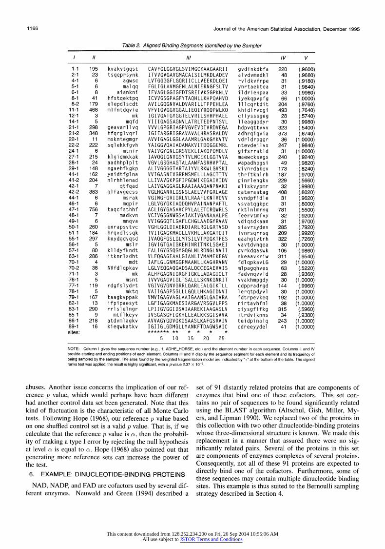
Table 2. Aligned Binding Segments Identified by the Sampler

I1 I Il IV V

1-1 195 kvakvtgqst CAVFGLGGVGLSVIMGCKAAGAARII gvdinkdkfa 220 (.9600) 2-1 23 tsqeprsynk ITVVGVGAVGMACAISILMKDLADEV alvdvmedkl 48 (.9680) 4-1 6 agwsc LVTGGGGFLGQRIICLLVEEKDLQEI rv]dkvfrpe 31 (.9180) 5-1 6 malqq FGLIGLAVMGENLALNIERNGFSLTV ynrtaektea 31 (.9840) 6-1 8 aiankni IFVAGLGGIGFDTSREIVKSGPKNLV ildrienpaa 33 (.9960) 8-1 41 hfstqektpq ICVVGSGPAGFYTAQHLLKHPQAHVD iyekqpvpfg 66 (1.0000) 8-2 179 elepd]scdt AVILGQGNVALDVARILLTPPEHLEA l]lcqrtdit 204 (.9760)

11-1 468 m]fntdqvie VFVIGVGGVGGALIEQIYRQQPWLKQ khid]rvcgi 493 (.7640) 12-1 3 mk IGIVGATGYGGTELVRILSHHPHAEE cilysssgeg 28 (.5740) 14-1 5 mqfd YIIIGAGSAGNVLATRLTEDPNTSVL ]leaggpdyr 30 (.9980) 21-1 298 geavar]lvq VVVLGPGRIAGPVGVEVDIVRDVEGA hdpvqttvvv 323 (.5400) 21-2 348 hfqrg]vqrl IGIEARGRIGRAVAVALHRASRALDV adhrqiqvia 373 (.6740) 22-1 11 mskntegmgr AVVIGAGLGGLAAAMRLGAKGYKVTV vdrldrpggr 36 (1.0000) 22-2 222 sqlekkfgvh YAIGGVQAIADAMAKVITDQGGEMRL ntevdeilvs 247 (.9840) 24-1 6 mtnir VAIVGYGNLGRSVEKLIAKQPDMDLV gifsrratld 31 (1.0000) 27-1 215 klgidmkkak IAVQGIGNVGSYTVLNCEKLGGTVVA maewcksegs 240 (.9240) 28-1 24 aadhhp]p]t VGVLGSGHAGTALAAWFASRHVPTAL wapadhpgsi 49 (.9820) 29-1 148 ngaehfkgkp ALIVGGGGTARTAIYVLRKWLGVSKI yivnrdakev 173 (.8240) 41-1 162 ynidtfg]na VVIGASNIVGRPMSMELLLAGCTTTV thrftknlrh 187 (.9700) 41-2 204 nlrhhlenad LLIVAVGKPGFIPGDWIKEGAIVIDV ginrlengkv 229 (.5660) 42-1 7 qtfqad LAIVGAGGAGLRAAIAAAQANPNAKI aliskvypmr 32 (.9980) 42-2 383 g]favgecss VGLHGANRLGSNSLAELVVFGRLAGE qateraatag 408 (.8020) 44-1 6 msrak VGINGFGRIGRLVLRAAFLKNTVDVV svndpfidle 31 (.9620) 46-1 6 mqpir LGLVGYGKIAQDQHVPAINANPAFTL vsvatqgkpc 31 (.8000) 47-1 756 taqcfsthhf ACLIGYGASAVCPYLALETCRQWRLS nktlnlmrng 781 (.5500) 48-1 7 madkvn VCIVGSGNWGSAIAKIVGANAAALPE feervtmfvy 32 (.9200) 49-1 6 mnqva VVIGGGQTLGAFLCHGLAAEGYRVAV vdiqsdkaan 31 (.9700) 50-1 260 enrapsvtvc VGHLGGLDIAERDIARLRGLGRTVSD siavrsydev 285 (.7920) 51-1 184 hrqvd]ssqk TVIIGAGKMACLLVKHLLAKGATDIT ivnrsqrrsq 209 (.9920) 55-1 297 knydgdvqsd IVAQGFGSLGLMTSILVTPDGKTFES eaahgtvtrh 322 (.7260) 56-1 5 ms]r IGVIGTGAIGKEHINRITNKLSGAEI vavtdvnqea 30 (1.0000) 57-1 80 kl]dyfkndt FALIGYGSQGYGQGLNLRDNGLNVII gvrkdgaswk 105 (.9860) 63-1 286 itknrlsdht VLFQGAGEAALGIANLIVMAMEKEGV skeaavkriw 311 (.9540) 70-1 4 mdt IAFLGLGNMGGPMAANLLKAGHRVNV fdlqpkavLG 29 (1.0000) 70-2 38 NVfdlqpkav LGLVEQGAQGADSALQCCEGAEVVIS m]pagqhves 63 (.5220) 71-1 3 mk ALHFGAGNIGRGFIGKLLADAGIQLT fadvnqvv]d 28 (.9360) 76-1 5 msnt IVVVGAGVIGLTSALLLSKNKGNKIT vvakhmpgdy 30 (1.0000) 77-1 119 rdgfslydrt VGIVGVGNVGRRLQARLEALGIKTLL cdppradrgd 144 (.9960) 78-1 5 mktq VAIIGAGPSGLLLGQLLHKAGIDNVI lerqtpdyvl 30 (1.0000) 79-1 167 taagkvppak VMVIGAGVAGLAAIGAANSLGAIVRA fdtrpevkeq 192 (1.0000) 82-1 13 ifpipaesyt LGFIGAGKMAESIARGAVRSGVLPPS rirtavhfnl 38 (1.0000) 83-1 290 rrlslelngr LPIIGVGGIDSVIAAREKIAAGASLV qiysgfifkg 315 (.5960) 85-1 9 mtflkeyv IVSGASGFIGKHLLEALKKSGISVVA itrdviknns 34 (.9380) 86-1 218 atdvm]agkv AVVAGYGDVGKGSAASLKAFGSRVIV teidpinalq 243 (1.0000) 89-1 16 kieqwkatkv IGIIGLGDMGLLYANKFTDAGWSVIC cdreeyydel 41 (1.0000) sites: ******* ** * * * *

5 10 15 20 25

NOTE: Column I gives the sequence number (e.g., 1, ADHE HORSE, etc.) and the element number in each sequence. Columns II and IV provide starting and ending positions of each element. Columns IlIl and V display the sequence segment for each element and its frequency of being sampled by the sampler. The sites found by the weighted fragmentation model are indicated by "*" at the bottom of the table. The signed ranks test was applied; the result is highly significant, with a p value 2.37 x 1 0-6.

abuses. Another issue concerns the implication of our reference p value, which would perhaps have been different had another control data set been generated. Note that this kind of fluctuation is the characteristic of all Monte Carlo tests. Following Hope (1968), our reference p value based on one shuffled control set is a valid p value. That is, if we calculate that the reference p value is ca, then the probability of making a type I error by rejecting the null hypothesis at level ca is equal to ca. Hope (1968) also pointed out that generating more reference sets can increase the power of the test.

6. EXAMPLE: DINUCLEOTIDE-BINDING PROTEINS

NAD, NADP, and FAD are cofactors used by several different enzymes. Neuwald and Green (1994) described a

set of 91 distantly related proteins that are components of enzymes that bind one of these cofactors. This set con- tains no pair of sequences to be found significantly related using the BLAST algorithm (Altschul, Gish, Miller, My- ers, and Lipman 1990). We replaced two of the proteins in this collection with two other dinucleotide-binding proteins whose three-dimensional structure is known. We made this replacement in a manner that assured there were no significantly related pairs. Several of the proteins in this set are components of enzymes complexes of several proteins. Consequently, not all of these 91 proteins are expected to directly bind one of the cofactors. Furthermore, some of these sequences may contain multiple dinucleotide binding sites. This example is thus suited to the Bernoulli sampling strategy described in Section 4.




The prior Dirichlet distributions for the frequencies of the 20 residue types for all site and nonsite positions were chosen so that the expected values of the frequencies were proportional to the composition of the entire data set. The pseudocounts (i.e., ca, + .+ ap or j + . ?/+ 3pj) were chosen as 9, 10% of the total number of sequences. Because we expected some proportion of the sequences to contain an element, we chose the parameters of the prior beta distribution in such a way that the expected number of elements was 45, corresponding to half an element per sequence, and with a standard deviation of our default value of 6, 3% of the mean. This gave us a = 180 and b = 144, 984. In this example the results do not change remarkably for different choices of (a, b) ranging from expected 1 element per se- 3 quence to one element per sequence. Because in this example the width of the motif is unknown, we applied fragmentation using the weighted prior with the defaults of J = 13 and W = 130. We applied the signed ranks test as described in Section 5 with the same prior distributions as those described earlier, except that we modified the beta parameters to correspond to a doubling of the expected number of elements. The sampler applied to the data set including the controls reported 38 elements that were sampled 50% of the iterations after convergence. Seven of these came from the control data set with a total rank of 55, which corresponds to a Z value of -4.6 using normal approximation with correction. In all cases we judged convergence in ac- cordance with the procedures described by Lawrence et al. (1993).

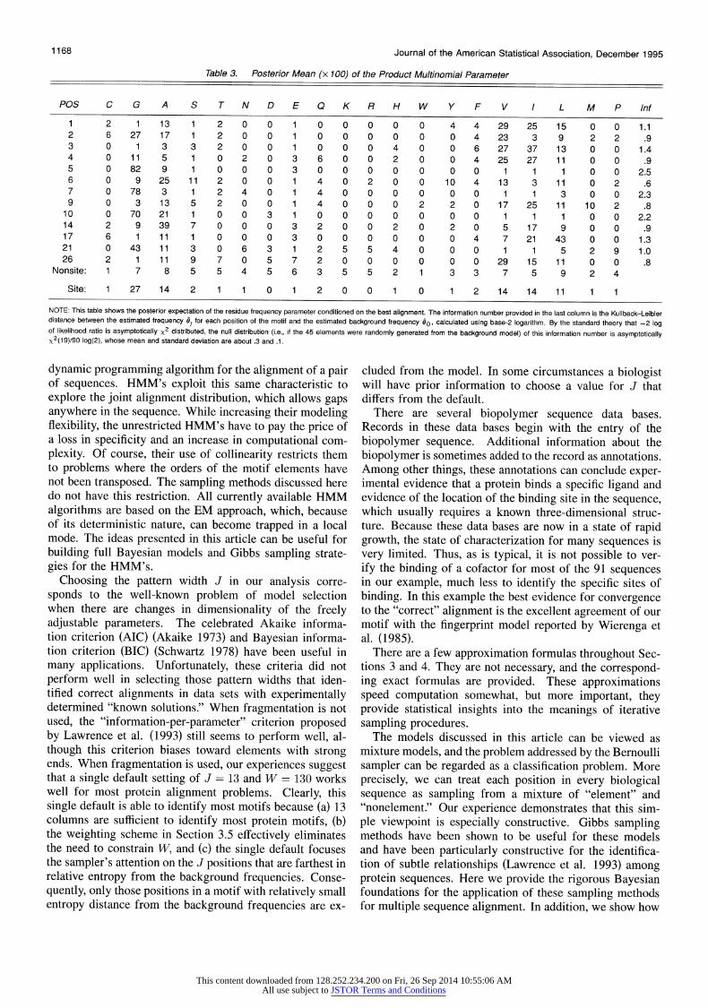
As shown in Table 2, 45 aligned elements from these 91 sequences were identified by the sampler. Table 3 gives the expected values of the a posteriori Dirichlet distributions associated with these aligned elements. Notice that the fragmentation model has selected a motif that spans 26 residues, and that this motif corresponds quite well with the strand- helix-strand motif of ADHE, as shown in Figure 3. It also corresponds to the locations of the known dinucleotide- binding strand-helix-strand structure in the two other proteins in this set for which such structural data are available. Furthermore, this motif corresponds nearly perfectly to a sequence fingerprint model for dinucleotide-binding segments derived by superimposing the structures of several of these proteins (Wierenga, DeMaeyer, and Hol 1985).

In protein motifs, not all of the positions are equally important. The last column in Table 3 gives the relative entropy (Cover and Thomas 1991) in bits (i.e., the Kullback- Leibler distance) between the site and nonsite models of the 13 sampled positions found for the motif. As these columns indicate, positions 5, 7, and 10 are the most dis- tant from the background model. All three positions are most frequently glycines, the smallest and most flexible of the 20 amino acids. In this motif, these three positions, which are colored red in Figure 3, play important distinct roles in the binding of NAD. The flexibility of a glycine residue at position 199 of ADHE (motif position 5) permits the protein chain to make the sharp bend shown in Fig- ure 3. The small size of a glycine at position 201 (motif position 7) permits the motif to closely approach the phosphate groups of NAD to which it binds. The small size of

the glycine at position 204 (motif position 10) permits the first strand of the strand-helix-strand structure to closely approach the helix. Position 3 of the motif (position 197 in ADHE), colored purple in Figure 3, is the fourth most dis- tant position. As indicated in Table 3, one of three residues (valine, isoleucine, or leucine) is required at this position. These three residue types are often found in the interior of a protein and help to stabilize a protein's structure. In this case this position helps to hold the first strand of this strand-helix-strand motif in position against the helix.

7. DISCUSSION

In most cases sequences available for analysis do not arise from a process that mimics independent samples from a common model, but rather they emerge by evolving from common ancestors. Some methods for sequence alignment that incorporate evolutionary history have been described (Allison et al. 1992; Bishop and Thompson 1986; Thorne et al. 1991, 1992), but the results from these in multiple sequence alignment have so far been limited. When sufficient diverse data are available, as in our dinucleotide- binding protein example, the independence assumption can be very closely achieved by removing highly correlated observations from the data set. In cases where there are in- sufficient data to take this approach, a method that can si- multaneously align a large set of sequences (especially sequences that include subtle relationships) and account for the correlations stemming from evolutionary history awaits future development. Although theory addressing these correlations is important, in practice we have found that the methods we propose here often work well even with substantial departures from the independence assumption. To date, our experience and that of others using these methods (S. Henikoff, personal communication) indicate that departures from the independence assumptions have nearly no impact on the methods described in Section 3. Although we have less experience with the method described in Section 4 (i.e., Bernoulli sampling methods), preliminary results indicate that this assumption is somewhat more important in this case.

Some basic similarities of this work with previously reported methods should be noted. Existing Gibbs sampling and EM algorithms for multiple sequence alignment share the treatment of alignment data as missing. Two EM approaches have been developed: one that finds alignments of ungapped elements (Cardon and Stormo 1992; Lawrence and Reilly 1990), the other in the form of hidden Markov models (HMM) that permit gaps between any two neigh- boring residues in a sequence (Baldi et al. 1994; Haussler et al. 1993). Because the joint distribution of multiple elements in each sequence must be explicitly estimated, the first approach has been limited to problems with only one or two motifs. The sampling methods permit us to escape this restriction by exploring the joint distribution through sampling the complete set of conditionals.

When sequence evolution has not been subject to duplications or transpositions, the order of the residues in the sequences will not be altered, and the sequences are said to be collinear. This collinearity induces a Markov relationship on the alignment, which forms the basis of a popular




Table 3. Posterior Mean (x 100) of the Product Multinomial Parameter

POS C G A S T N D E 0 K R H W Y F V I L M P Inf

1 2 1 13 1 2 0 0 1 0 0 0 0 0 4 4 29 25 15 0 0 1.1 2 6 27 17 1 2 0 0 1 0 0 0 0 0 0 4 23 3 9 2 2 .9 3 0 1 3 3 2 0 0 1 0 0 0 4 0 0 6 27 37 13 0 0 1.4 4 0 11 5 1 0 2 0 3 6 0 0 2 0 0 4 25 27 11 0 0 .9 5 0 82 9 1 0 0 0 3 0 0 0 0 0 0 0 1 1 1 0 0 2.5 6 0 9 25 11 2 0 0 1 4 0 2 0 0 10 4 13 3 11 0 2 .6 7 0 78 3 1 2 4 0 1 4 0 0 0 0 0 0 1 1 3 0 0 2.3 9 0 3 13 5 2 0 0 1 4 0 0 0 2 2 0 17 25 11 10 2 .8

10 0 70 21 1 0 0 3 1 0 0 0 0 0 0 0 1 1 1 0 0 2.2 14 2 9 39 7 0 0 0 3 2 0 0 2 0 2 0 5 17 9 0 0 .9 17 6 1 11 1 0 0 0 3 0 0 0 0 0 0 4 7 21 43 0 0 1.3 21 0 43 11 3 0 6 3 1 2 5 5 4 0 0 0 1 1 5 2 9 1.0 26 2 1 11 9 7 0 5 7 2 0 0 0 0 0 0 29 15 11 0 0 .8

Nonsite: 1 7 8 5 5 4 5 6 3 5 5 2 1 3 3 7 5 9 2 4

Site: 1 27 14 2 1 1 0 1 2 0 0 1 0 1 2 14 14 11 1 1

NOTE: This table shows the posterior expectation of the residue frequency parameter conditioned on the best alignment. The information number provided in the last column is the Kullback-Leibler distance between the estimated frequency e, for each position of the motif and the estimated background frequency 60, calculated using base-2 logarithm. By the standard theory that -2 log of likelihood ratio is asymptotically x2 distributed, the null distribution (i.e., if the 45 elements were randomly generated from the background model) of this information number is asymptotically x2(19)/90 log(2), whose mean and standard deviation are about .3 and .1.

dynamic programming algorithm for the alignment of a pair of sequences. HMM's exploit this same characteristic to explore the joint alignment distribution, which allows gaps anywhere in the sequence. While increasing their modeling flexibility, the unrestricted HMM's have to pay the price of a loss in specificity and an increase in computational com- plexity. Of course, their use of collinearity restricts them to problems where the orders of the motif elements have not been transposed. The sampling methods discussed here do not have this restriction. All currently available HMM algorithms are based on the EM approach, which, because of its deterministic nature, can become trapped in a local mode. The ideas presented in this article can be useful for building full Bayesian models and Gibbs sampling strategies for the HMM's.

Choosing the pattern width J in our analysis corresponds to the well-known problem of model selection when there are changes in dimensionality of the freely adjustable parameters. The celebrated Akaike information criterion (AIC) (Akaike 1973) and Bayesian information criterion (BIC) (Schwartz 1978) have been useful in many applications. Unfortunately, these criteria did not perform well in selecting those pattern widths that identified correct alignments in data sets with experimentally determined "known solutions." When fragmentation is not used, the "information-per-parameter" criterion proposed by Lawrence et al. (1993) still seems to perform well, although this criterion biases toward elements with strong ends. When fragmentation is used, our experiences suggest that a single default setting of J= 13 and W = 130 works well for most protein alignment problems. Clearly, this single default is able to identify most motifs because (a) 13 columns are sufficient to identify most protein motifs, (b) the weighting scheme in Section 3.5 effectively eliminates the need to constrain W, and (c) the single default focuses the sampler's attention on the J positions that are farthest in relative entropy from the background frequencies. Conse- quently, only those positions in a motif with relatively small entropy distance from the background frequencies are ex-

cluded from the model. In some circumstances a biologist will have prior information to choose a value for J that differs from the default.

There are several biopolymer sequence data bases. Records in these data bases begin with the entry of the biopolymer sequence. Additional information about the biopolymer is sometimes added to the record as annotations. Among other things, these annotations can conclude exper- imental evidence that a protein binds a specific ligand and evidence of the location of the binding site in the sequence, which usually requires a known three-dimensional structure. Because these data bases are now in a state of rapid growth, the state of characterization for many sequences is very limited. Thus, as is typical, it is not possible to ver- ify the binding of a cofactor for most of the 91 sequences in our example, much less to identify the specific sites of binding. In this example the best evidence for convergence to the "correct" alignment is the excellent agreement of our motif with the fingerprint model reported by Wierenga et al. (1985).

There are a few approximation formulas throughout Sec- tions 3 and 4. They are not necessary, and the corresponding exact formulas are provided. These approximations speed computation somewhat, but more important, they provide statistical insights into the meanings of iterative sampling procedures.

The models discussed in this article can be viewed as mixture models, and the problem addressed by the Bernoulli sampler can be regarded as a classification problem. More precisely, we can treat each position in every biological sequence as sampling from a mixture of "element" and "nonelement." Our experience demonstrates that this simple viewpoint is especially constructive. Gibbs sampling methods have been shown to be useful for these models and have been particularly constructive for the identification of subtle relationships (Lawrence et al. 1993) among protein sequences. Here we provide the rigorous Bayesian foundations for the application of these sampling methods for multiple sequence alignment. In addition, we show how




to extend these methods by relaxing the specification of the number and size of motifs. Furthermore, we develop a ranks test to judge the statistical significance of a multiple alignment.

APPENDIX: WEIGHTED SAMPLING FROM FINITE POPULATION

The conditional distribution (7) can be regarded as a generalized Bernoulli-Laplace model; that is, the one for drawing a sample of size J from a pool of W weighted balls without replacement, such that the joint probability of the J balls is proportional to the product of their respective weights. Chen, Dempster, and Liu (1994) explained how this is a maximum entropy model and presented efficient algorithms to generate the sample sequentially. Because our use of the model is nested in a general Gibbs sampling procedure, an iterative scheme is sufficient.

The sampling strategy that we designed is equivalent to a Markov chain evolving in the following way. Let 1t = {il, ...Iij} denote a sample of J balls at step t. At step t + 1, a ball (say, i1) is first drawn from 1t with equal probability and excluded from the sample Ft; then a ball (say, i*) is picked from the pool FP' U {ii } with probability proportional to its weight. So ]Ft+i = \ {ii} U {i* }. This Markov chain is reversible with 7r* as its equilibrium distribution and is related to the Metropolis scheme of Chen et al. (1994).

Instead of excluding a ball from the current sample 1t completely at random, we may want to draw one in proportional to gi-1 for i E 1t. We call this strategy doubly proportional sampling. The equilibrium distribution of this new strategy is found to be

2 W

tr t(A)o a H gi2 E wgwl) II6,=1 w=l

To see why, consider a configuration Y { {1, .. J} and let Xik = Y \ {i} U {k}, where i < J and k > J. So Xik differs from Y by one element. The transition functions are

T(Y, Y) {~= 3 }{ZJl?gi}g i=1 { 3g, Ig Ek= J ;9gk + gi}

and

( -1 } { }

Then it is easy to check J W

E E 7t (X,k)T(Xik, Y) + 7t (Y)T(Y, Y) =

-7t (Y

i=1 k=J+l

so that the 7rt is indeed invariant under the foregoing transition. A general doubly proportional sampling chain M,,g can be

defined as follows: At step t + 1, a ball (say, ik) from Ft = {ii, ... , ij } is chosen to be excluded with probability proportional to the g' ; then a ball is drawn from the pool IF' U {ik } with probability proportional to the g, for j E 1t' U {ik }. The equilibrium distribution of this procedure is

irt(r) ?F>xf{g } {Z g7

jEr jEr

as can be verified by examination of the equilibrium equation as shown previously. By choosing different Ol and /, we were able to obtain different equilibrium distributions. A further general- ization can be easily made to the case when two sets of weights,

{a,, . ., aj} and {bl,. . , bj}, are used for the two proportional sampling steps.

[Received January 1994. Revised April 1995.]

REFERENCES

Akaike, H. (1973), "Information Theory and the Maximum Likelihood Principle," in 2nd International Symposium on Information Theory, eds. B. N. Petrov and F. Csaki, Budapest: Akademiai Ki'ado.

Allison, L., Wallace, C. S., and Yee, C. N. (1992), "Minimum Message Length Encoding Evolutionary Trees and Multiple Alignment," in Pro- ceedings of 25th Hawaii International Conference on System Science, pp. 663-674.

Altschul, S. F., Gish, W., Miller, M., Myers, E. W., and Lipman, D. J. (1990), "Basic Local Alignment Search Tool," Journal of Molecular Biology, 215, 403-410.

Baldi, P., Chauvin, Y., McClure, M., and Hunkapiller, T. (1994), "Hidden Markov Models of Biological Primary Sequence Information," in Pro- ceedings of the National Academy of Science of USA, 91, 1059-1063.

Berg, 0. G., and von Hipple, P. H. (1987), "Selection of DNA Binding Sites by Regulatory Proteins: Statistical-Mechanical Theory and Application to Operators and Promoters," Journal of Molecular Biology, 193, 153- 161.

Bishop, M. J., and Thompson, E. A. (1986), "Maximum Likelihood Align- ment of DNA Sequences," Journal of Molecular Biology, 190, 159-165.

Bryant, S. H., and Lawrence, C. E. (1991), "The Frequencies of Ion Pair Substructures in Proteins Is Quantitatively Related to Electrostatic Po- tentials: A Statistical Model for Nonbonded Interactions," PROTEINS: Structure, Function, and Genetics, 9, 108-119.

(1993), "An Empirical Energy Function for Threading Protein Se- quence Through the Folding Motif," PROTEINS: Structure, Function, and Genetics, 16, 92-112.

Cardon, L. R., and Stormo, G. D. (1992), "An Expectation Maximization Algorithms for Identifying Protein Binding Sites With Variable Gaps From Unaligned DNA Fragments," Journal of Molecular Biology, 223, 159-170.

Chen, R., and Liu, J. S. (1996), "Predictive Updating Methods With Ap- plications to Bayesian Classification," Journal of the Royal Statistical Society, Ser. B, to appear.

Chen, X., Dempster, A. P., and Liu, J. S. (1994), "Weighted Finite Popu- lation Sampling to Maximize Entropy," Biometrika, 457-469.

Cover, T. M., and Thomas, J. A. (1991), Elements of Information Theory, New York: John Wiley.

Gelfand, A. E., and Smith, A. F. M. (1990), "Sampling-Based Approaches to Calculating Marginal Densities," Journal of the American Statistical Association, 85, 398-409.

Gelman, A., and Rubin, D. B. (1992), "Inference From Iterative Simulation Using Multiple Sequences," Statistical Science, 7, 457-472.

Haussler, D., Krogh, A., Mian, S., and Sjolander, K. (1993), "Protein Mod- eling Using Hidden Markov Models: Analysis of Globins," in Proceed- ings of the Hawaii International Conference on System Sciences, Los Alamitos, CA: IEEE Computer Society Press.

Hope, A. C. A. (1968), "A Simplified Monte Carlo Significance Test Pro- cedure," Journal of the Royal Statistical Society, Ser. B, 30, 582-598.

Lawrence, C. E., Altschul, S. F., Boguski, M. S., Liu, J. S., Neuwald, A. F., and Wootton, J. C. (1993), "Detecting Subtle Sequence Signals: A Gibbs Sampling Strategy for Multiple Alignment," Science, 262, 208-314.

Lawrence, C. E., and Reilly, A. A. (1990), "An Expectation Maximization Algorithm for the Identification and Characterization of Common Sites in Unaligned Biopolymer Sequences," PROTEINS: Structure, Function, and Genetics, 7, 41-51.

(1992), "Likelihood Inferences With Uncertain Indices With Ap- plication to Gene Regulation," Technical Report 121, Biometrics Lab- oratory, Wadsworth Center for Laboratories and Research, New York State Department of Health.

Li, K.-H. (1988), "Imputation Using Markov Chains," Journal of Statistical Computation and Simulation, 30, 57-79.

Lipman, D. J., Wilbur, W. J., Smith, T. F., and Waterman, M. S. (1984), "On the Statistical Significance of Nucleic Acid Similarities," Nucleic Acids Research, 12, 215-326.




Liu, J. S. (1994), "The Collapsed Gibbs Sampler in Bayesian Computa- tions With Applications to a Gene Regulation Problem," Journal of the American Statistical Association, 89, 958-966.

Liu, J. S., Wong, W. H., and Kong, A. (1994), "Covariance Structure of the Gibbs Sampler With Applications to the Comparisons of Estimators and Augmentation Schemes," Biometrika, 81, 27-40.

(1995), "Covariance Structure and Convergence Rate of the Gibbs Sampler With Various Scans," Journal of the Royal Statistical Society, Ser. B, 56, 157-169.

Neuwald, A. F., and Green, P. (1994), "Detecting Patterns in Protein Se- quences," Journal of Molecular Biology, 239, 698-712.

Neuwald, A. F., Liu, J. S., and Lawrence, C. E. (1995), "Sequence Analysis Using a Motif Sampling Strategy," submitted to Protein Science.

Pohl, F. M. (1971), "Empirical Protein Energy Maps," Nature: New Biol- ogy, 234, 277-379.

Schwartz, G. (1978), "Estimating the Dimension of a Model," The Annals

of Statistics, 6, 461-464. Tanner, M. A., and Wong, W. H. (1987), "The Calculation of Posterior

Distribution by Data Augmentation," (with discussion), Journal of the American Statistical Association, 82, 528-550.

Thorne, J. L., Kishino, H., and Felsenstein, J. (1991), "An Evolutionary Model for Maximum Likelihood Alignment of DNA Sequences," Jour- nal of Molecular Evolution, 33, 114-124.

(1992), "Inching Toward Reality: An Improved Likelihood Model of Sequence Evolution," Journal of Molecular Evolution, 34, 3-16.

Tierney, L. (1995), "Markov Chains for Exploring Posterior Distributions (with discussion)," The Annals of Statistics, 22, 1701-1762.

Wierenga, R. K., DeMaeyer, M. C. H., and Hol, W. G. J. (1985), "Inter- action of Pyrophosphate Moieties With Alpha-Helixes in Dinucleotide Binding Proteins," Biochemistry, 24, 1346-1357.

Wilcoxon, F. (1945), "Individual Comparisons by Ranking Methods," Bio- metrics, 1, 80-83.



bayesian models for multiple local sequence alignment...

Documents