bayesian networks inference in bayesian networksdprecup/courses/ml/... · lecture 8: bayesian...
TRANSCRIPT
Lecture 8: Bayesian Networks
• Bayesian Networks
• Inference in Bayesian Networks
COMP-652 and ECSE 608, Lecture 8 - January 31, 2017 1

Bayes nets
0.65P(C|A)
C=0
A=0
A=1
0.05 0.95
0.7 0.3
C=1
P(B)
B=1 B=0
0.01 0.99
B=0,E=0
B=0,E=1
B=1,E=0
B=1,E=1
A=1 A=00.001 0.9990.3
0.8
0.95
0.7
0.05
0.2
P(A|B,E)
E B
A
C
R
P(E)
E=1 E=0
0.9950.005
P(R|E)
R=1
E=0
E=1
R=0
0.99990.0001
0.35
• The nodes represent random variables
• The arcs represent “influences”
• At each node, we have a conditional probability distribution (CPD) forthe corresponding variable given its parents
COMP-652 and ECSE 608, Lecture 8 - January 31, 2017 2

Factorization
• Let G be a DAG over random variables variables X1, . . . , Xn
• We say that a joint probability distribution P factorizes according to Gif it can be expressed as a product:
P (x1, . . . , xn) =
n∏i=1
p(xi|xπi),∀xi ∈ Dom(Xi)
where Xπi denotes the parents of Xi in the graph
• The individual factors P (Xi|Xπi) are called local probabilistic models orconditional probability distributions (CPD)
• Naive Bayes and Gaussian discriminant models are special cases of thistype of model
COMP-652 and ECSE 608, Lecture 8 - January 31, 2017 3

Complexity of a factorized representation
• If k is the maximum number of ancestors for any node in the graph, andwe have binary variables, then every conditional probability distributionwill require ≤ 2k numbers to specify
• The whole joint distribution can then be specified with ≤ n ·2k numbers,instead of 2n
• The savings are big if the graph is sparse (k � n).
COMP-652 and ECSE 608, Lecture 8 - January 31, 2017 4

Types of local parametrization
• Tables (if both parents and the node are discrete)
• Tree-structured CPDs (if all nodes are discrete, but the conditional isnot always dependent on all the parents)
• Gaussians (for continuous variables)
• Mixture of Gaussians
• ....
COMP-652 and ECSE 608, Lecture 8 - January 31, 2017 5
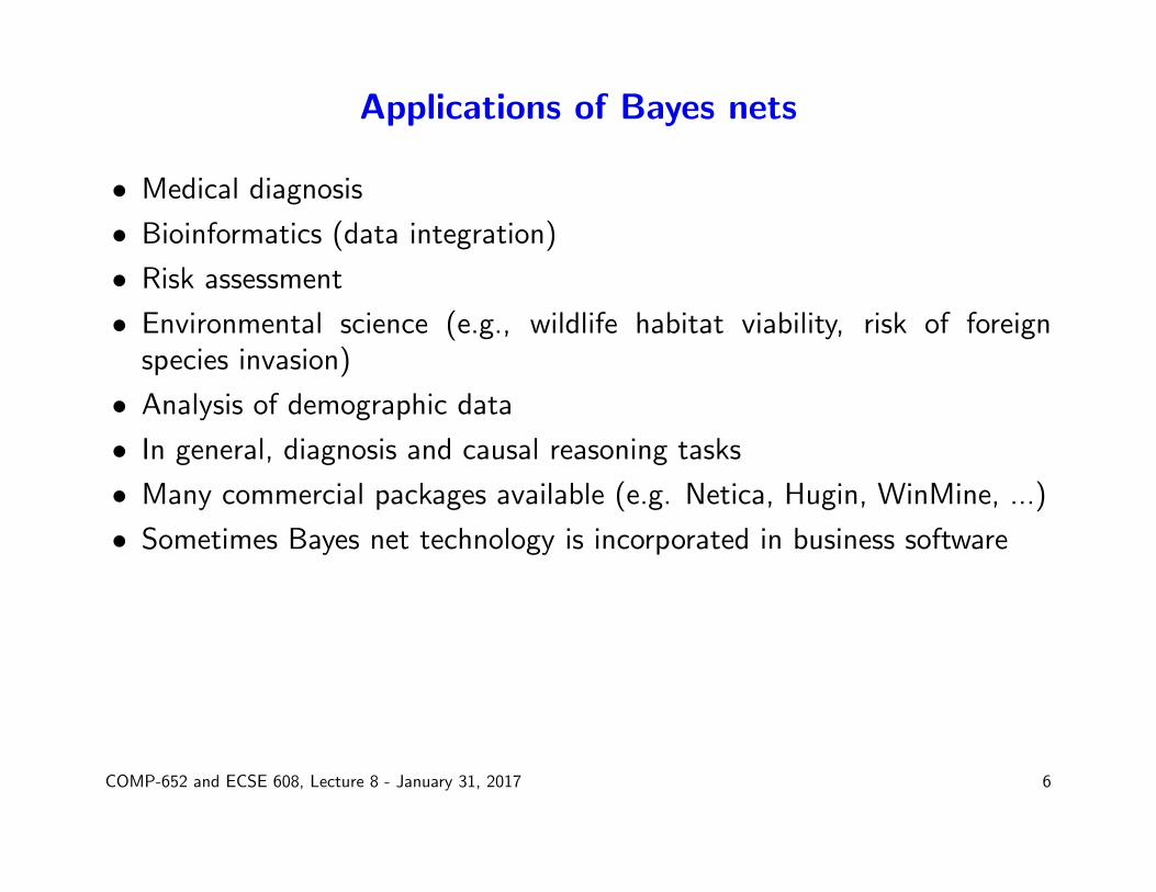
Applications of Bayes nets
• Medical diagnosis
• Bioinformatics (data integration)
• Risk assessment
• Environmental science (e.g., wildlife habitat viability, risk of foreignspecies invasion)
• Analysis of demographic data
• In general, diagnosis and causal reasoning tasks
• Many commercial packages available (e.g. Netica, Hugin, WinMine, ...)
• Sometimes Bayes net technology is incorporated in business software
COMP-652 and ECSE 608, Lecture 8 - January 31, 2017 6

Example: Pathfinder (Heckermann, 1991)
• Medical diagnostic system for lymph node diseases
• Large net! 60 diseases, 100 symptoms and test results, 14000 probabilities
• Network built by medical experts
– 8 hours to determine the variables– 35 hours for network topology– 40 hours for probability table values
• Experts found it easy to invent causal links and probabilities
• Pathfinder is now outperforming world experts in diagnosis
• Commercialized by Intellipath and Chapman Hall Publishing; extendedto other medical domains
COMP-652 and ECSE 608, Lecture 8 - January 31, 2017 7

Implied independencies in Bayes nets: “Markov chain”YX Z
• Think of X as the past, Y as the present and Z as the future• This is a simple Markov chain• Based on the graph structure, we have:
p(X,Y, Z) = p(X)p(Y |X)p(Z|Y )
• Hence, we have:
p(Z|X,Y ) =p(X,Y, Z)
p(X,Y )=p(X)p(Y |X)p(Z|Y )
p(X)p(Y |X)= p(Z|Y )
Hence, X⊥⊥Z|Y• Note that the edges that are present do not imply dependence. But the
edges that are missing do imply independence.
COMP-652 and ECSE 608, Lecture 8 - January 31, 2017 8

Implied independencies in Bayes nets: “Common cause”
Z
Y
X
p(X|Y,Z) =p(X,Y, Z)
p(Y,Z)=p(Y )p(X|Y )p(Z|Y )
p(Y )p(Z|Y )= p(X|Y )
• Based on this, X⊥⊥Z|Y .
• This is a “hidden variable” scenario: if Y is unknown, then X and Zcould appear to be dependent on each other
COMP-652 and ECSE 608, Lecture 8 - January 31, 2017 9
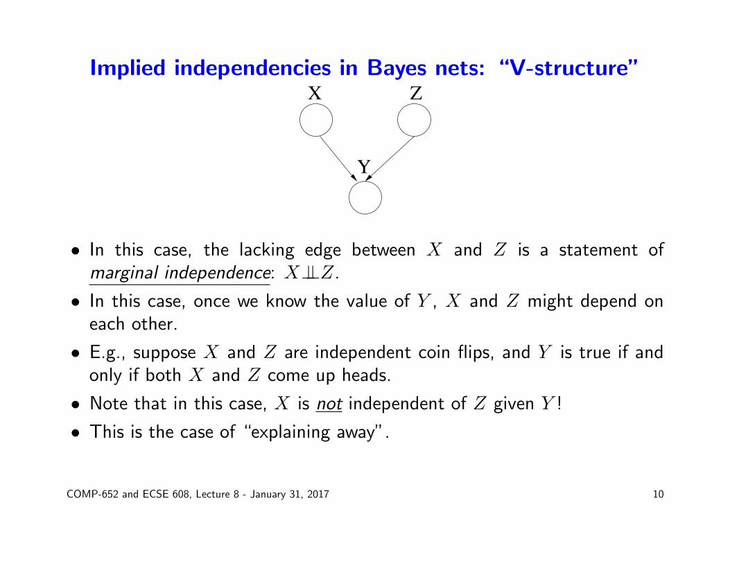
Implied independencies in Bayes nets: “V-structure”
Y
X Z
• In this case, the lacking edge between X and Z is a statement ofmarginal independence: X⊥⊥Z.
• In this case, once we know the value of Y , X and Z might depend oneach other.
• E.g., suppose X and Z are independent coin flips, and Y is true if andonly if both X and Z come up heads.
• Note that in this case, X is not independent of Z given Y !
• This is the case of “explaining away”.
COMP-652 and ECSE 608, Lecture 8 - January 31, 2017 10

Rules for information propagationRecall: Base rules for propagating information
• Head-to-tail
Y known, path blocked
X Y Z X Y Z
Y unknown, path unblocked
• Tail-to-tail
Y known, path blocked
Y
X Z
Y
X Z
Y unknown, path unblocked
• Head-to-head
Y known, path UNBLOCKED
X Z
Y
X Z
Y
Y unknown, path BLOCKED
January 11, 2008 3 COMP-526 Lecture 4COMP-652 and ECSE 608, Lecture 8 - January 31, 2017 11

Markov blanket of a node
• Suppose we want the smallest set of nodes U such that X is independentof all other nodes in the network given U . What should U be?
• Clearly, at least X’s parents and children should be in U
• But this is not enough if there are v-structures; U will also have toinclude X’s “spouses” - i.e. the other parents of X’s children
• The set U consisting of X’s parents, children and other parents of itschildren is called the Markov blanket of X.
Markov blanket
• Clearly, at least X ’s parents and children should be in U
• But this is not enough if there are v-structures; U will also haveto include X ’s “spouses” - i.e. the other parents of X ’s children
The set U consisting of X ’s parents, children and other parents ofits children is called the Markov blanket of X .
X
January 11, 2008 8 COMP-526 Lecture 4COMP-652 and ECSE 608, Lecture 8 - January 31, 2017 12

Moral graphs
• Given a DAG G, we define the moral graph of G to be an undirectedgraph U over the same set of vertices, such that the edge (X,Y ) is inU if X is in Y ’s Markov blanket
• Many independencies are lost in the moral graph
• Moral graphs will prove to be useful when we talk about inference.
Moral graphs
Given a DAG G, we define the moral graph of G to be anundirected graph U over the same set of vertices, such that theedge (X, Y ) is in U if X is in Y ’s Markov blanket
• If G is an I-map of p, then U will also be an I-map of p• But many independencies are lost when going to a moral graph• Moral graphs will prove to be useful when we talk aboutinference.
January 11, 2008 9 COMP-526 Lecture 4
COMP-652 and ECSE 608, Lecture 8 - January 31, 2017 13

Inference in Bayes nets
• Exact inference
– Variable elimination– Belief propagation
• Approximate inference
– Loopy belief propagation– Rejection sampling– Likelihood weighting (a for of importance sampling)– Gibbs sampling– Variational methods
COMP-652 and ECSE 608, Lecture 8 - January 31, 2017 14

Applying belief propagation to Bayes nets
1. Construct an undirected model corresponding to the Bayes net, by“moralizing” the graph
2. Potential functions can be constructed based on the original probabilities
3. Use belief propagation (on the junction tree, or the loopy version) on theundirected graph
4. Alternatively, use the information propagation rules to transmit messages
COMP-652 and ECSE 608, Lecture 8 - January 31, 2017 15

Belief propagation on treesBelief propagation on trees
(I,S)
(K,C)
Directed model
K
SC
B W
Undirected model
p(K)
p(S|K)
p(W|C)
p(C|K)
Kids
Chaos Sleep
WorkBills
p(B|C)!(B,C) !(W,C)
!(K,S)
!!""
Immunity
p(I|S)
I
!
!
We can parameterize the corresponding undirected model by:
Ψ(root) = p(root) and Ψ(xj, xi) = p(xj|xi)
for any nodes such that Xi is the parent of Xj
COMP-652, Lecture 19 - November 20, 2012 34
We can parameterize the corresponding undirected model by:
Ψ(root) = p(root) and Ψ(xj, xi)
for any nodes such that Xi is the parent of Xj
COMP-652 and ECSE 608, Lecture 8 - January 31, 2017 16

Introducing evidence
Order: B,W,C,K,I,S
S
C
WB
IK
P(S|B=0)=?
• If we want to compute p(Y |E), we introduce the evidence potentialδ(xi, x̂i), for all evidence variables Xi ∈ E• The potentials now become:
ψE(xi) =
{ψ(xi)δ(xi, x̂i) if Xi ∈ Eψ(xi), otherwise
• Traverse the tree starting at the leaves, propagating evidence
COMP-652 and ECSE 608, Lecture 8 - January 31, 2017 17

What are the messages?
B
(C)mBC
(K)mCK
(S)mKS(S)mIS
(C)mWCC
K
S
I
W
The message passed by C to K will be:
mCK(K) =∑c
(ψE(c)ψ(c, k)mBC(c)mWC(c)
)where mBC(C) and mWC(C) are the messages from B and C.
COMP-652 and ECSE 608, Lecture 8 - January 31, 2017 18

Belief propagation updates
• Node Xj computes the following message for node Xi
mji(xi) =∑xj
ψE(xj)ψ(xi, xj)∏
k∈neighbors(xj)−{xi}
mkj(xj)
Note that it aggregates the evidence of Xj itself, the evidence receivedfrom all neighbors except Xi, and “modulates” it by the potentialbetween Xj and Xi.
• The desired query probability is computed as:
p(y|x̂E) ∝ ψE(y)∏
k∈neighbors(Y )
mky(y)
COMP-652 and ECSE 608, Lecture 8 - January 31, 2017 19

Computing all probabilities simultaneously
B
C
K
S
I
W
• Because messages can be re-used, we can compute all conditionalprobabilities by computing all messages!
• Note that the number of messages is not too big
• We can use our previous equations to compute messages, but we need aprotocol for when to compute them
COMP-652 and ECSE 608, Lecture 8 - January 31, 2017 20
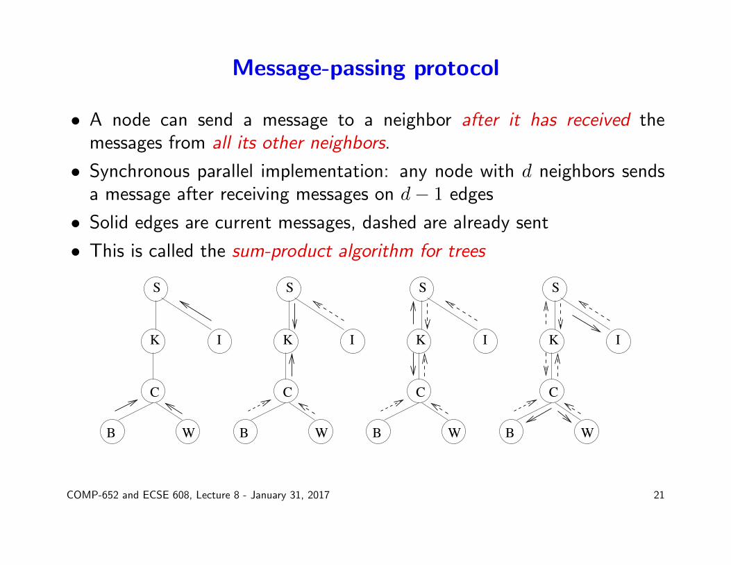
Message-passing protocol
• A node can send a message to a neighbor after it has received themessages from all its other neighbors.
• Synchronous parallel implementation: any node with d neighbors sendsa message after receiving messages on d− 1 edges
• Solid edges are current messages, dashed are already sent
• This is called the sum-product algorithm for trees
B
C
K
S
I
W B
C
K
S
I
W B
C
K
S
I
W B
C
K
S
I
W
COMP-652 and ECSE 608, Lecture 8 - January 31, 2017 21

Using the tree algorithm - take 1
• Turn the undirected moral graph into a tree!
• Then just use the tree algorithm
• The catch: the graph needs to be triangulated
D
A B
C• Finding an optimal triangulation in general is NP-hard
• Usually not the preferred option...
COMP-652 and ECSE 608, Lecture 8 - January 31, 2017 22

Using the tree algorithm - take 2
• Simply keep computing and propagating messages!
• At node Xj, re-compute the message as:
mnewij (xj) =
∑xi
ψ(Xi, Xj)ψ(Xi)∏
k∈Neighbors(i),k 6=j
moldki (xi)
• Note that the last two factors are only a function of Xi
• This is called loopy belief propagation
COMP-652 and ECSE 608, Lecture 8 - January 31, 2017 23
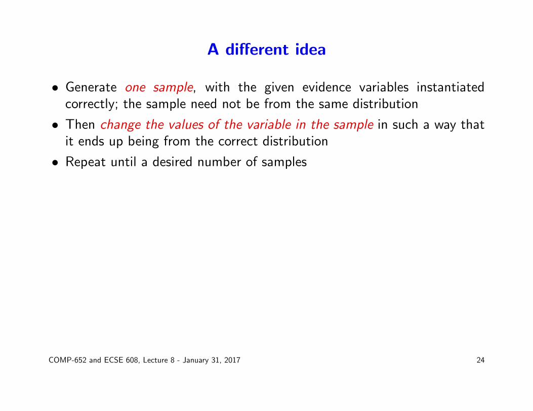
A different idea
• Generate one sample, with the given evidence variables instantiatedcorrectly; the sample need not be from the same distribution
• Then change the values of the variable in the sample in such a way thatit ends up being from the correct distribution
• Repeat until a desired number of samples
COMP-652 and ECSE 608, Lecture 8 - January 31, 2017 24

Gibbs sampling for Bayes nets
1. Initialization
• Set evidence variables E, to the observed values e• Set all other variables to random values (e.g. by forward sampling)
This gives us a sample x1, . . . , xn.
2. Repeat (as much as wanted)
• Pick a non-evidence variable Xi uniformly randomly)• Sample x′i from P (Xi|x1, . . . , xi−1, xi+1, . . . , xn).• Keep all other values: x′j = xj,∀j 6= i• The new sample is x′1, . . . , x
′n
3. Alternatively, you can march through the variables in some predefinedorder
COMP-652 and ECSE 608, Lecture 8 - January 31, 2017 25

Why Gibbs works in Bayes nets
• The key step is sampling according to P (Xi|x1, . . . , xi−1, xi+1, . . . , xn).How do we compute this?
• In Bayes nets, we know that a variable is conditionally independent of allothers given its Markov blanket (parents, children, spouses)
P (Xi|x1, . . . , xi−1, xi+1, . . . , xn) = P (Xi|MarkovBlanket(Xi))
• So we need to sample from P (Xi|MarkovBlanket(Xi))
• Let Yj, j = 1, . . . , k be the children of Xi. It is easy to show that:
P (Xi = xi|MarkovBlanket(Xi)) ∝ P (Xi = xi|Parents(Xi)) ·
·k∏j=1
P (Yj = yj|Parents(Yj))
COMP-652 and ECSE 608, Lecture 8 - January 31, 2017 26
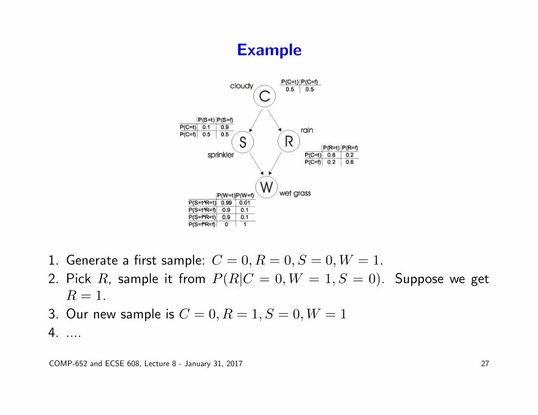
Example
1. Generate a first sample: C = 0, R = 0, S = 0,W = 1.
2. Pick R, sample it from P (R|C = 0,W = 1, S = 0). Suppose we getR = 1.
3. Our new sample is C = 0, R = 1, S = 0,W = 1
4. ....
COMP-652 and ECSE 608, Lecture 8 - January 31, 2017 27

Analyzing Gibbs sampling
• Consider the variables X1, . . . , Xn. Each possible assignment of valuesto these variables is a state of the world, 〈x1, . . . , xn〉.• In Gibbs sampling, we start from a given state s = 〈x1, . . . , xn〉. Based
on this, we generate a new state, s′ = 〈x′1, . . . , x′n〉.• s′ depends only on s!
• There is a well-defined probability of going from s to s′.
• Gibbs sampling constructs a Markov chain over the Bayes net
COMP-652 and ECSE 608, Lecture 8 - January 31, 2017 28

Recall: Markov chains
• Suppose you have a system which evolves through time:s0 → s1 → · · · → st → st+1 → . . .
• A Markov chain is a special case of such a system, defined by:
– A set of states S– A starting distribution over the set of states p0(s) = P (s0 = s). If the
state space is discrete, this can be represented as a column vector p0
– A stationary transition probability, specifying ∀s, s′ ∈ S, pss′ =P (st+1 = s′|st = s). The Markov property here means thatP (st+1|st) = P (st+1|s0, . . . st).
• For convenience, we put these probabilities in a |S|×|S| transition matrixT.
COMP-652 and ECSE 608, Lecture 8 - January 31, 2017 29

How does the chain evolve over time?
• Where will the chain be on the first time step, t = 1?
P (st+1 = s′) =∑s
P (s0 = s)P (s1 = s′|s0 = s)
by using the graphical model for the first time step: s0 → s1.
• We can put this in matrix form as follows:
p′1 = p′0T −→ p1 = T′p0
where T′ denotes the transpose of T
• Similarly, at t = 2, we have:
p2 = T′p1 = (T′)2p0
COMP-652 and ECSE 608, Lecture 8 - January 31, 2017 30

Steady-state (stationary) distribution
• By induction, the probability distribution over possible states at timestep t can be computed as:
pt = T′pt−1 = (T′)tp0
• If limt→∞pt exists, it is called the stationary or steady-state distributionof the chain.
• If the limit exists, π = limt→∞pt, then we have:
π = T′π,∑s∈S
πs = 1
• Under what conditions does a chain have a stationary distribution?
• Does the equation π = T′π always have a unique solution?
COMP-652 and ECSE 608, Lecture 8 - January 31, 2017 31

Not all chains have a stationary distribution
• If the chain has a purely periodic cycle, the stationary distribution doesnot exist
• E.g. the system is always in one state on odd time steps and the otherstate on even time steps, so the probability vector pt oscillates between2 values
• For the limit to exist, the chain must be aperiodic
• A standard trick for breaking periodicity is to add self-loops with smallprobability
COMP-652 and ECSE 608, Lecture 8 - January 31, 2017 32

Limit distribution may depend on the initial transition
• If the chain has multiple “components”, the limit distribution may exist,but depend on a few initial steps
• Such a chain is called reducible
• To eliminate this, every state must be able to reach every other state:
∀s, s′,∃k > 0 s.t. P (st+k = s′|st = s) > 0
COMP-652 and ECSE 608, Lecture 8 - January 31, 2017 33

Ergodicity
• An ergodic Markov chain is one in which any state is reachable from anyother state, and there are no strictly periodic cycles (in other words, thechain is irreducible and aperiodic)
• In such a chain, there is a unique stationary distribution π, which can beobtained as:
π = limt→∞
pt
This is also called the equilibrium distribution
• The chain reaches the equilibrium distribution regardless of p0
• The distribution can be computed by solving:
π = T′π,∑s
πs = 1
COMP-652 and ECSE 608, Lecture 8 - January 31, 2017 34

Balance in Markov chains
• Consider the steady-state equation for a system of n states:
[π1π2 . . . πn] = [π1π2 . . . πn]
1−∑i6=1 p1i p12 . . . p1n
p21 1−∑i6=2 p2i. . . p2n. . . . . . . . . . . .pn1 pn2 . . . 1−∑i6=n pni
• By doing the multiplication, for any state s, we get:
πs = πs
1−∑i6=s
psi
+∑i6=s
πipis =⇒ πs∑i6=s
psi =∑i6=s
πipis
This can be viewed as a “flow” property: the flow out of s has to beequal to the flow coming into s from all other states
COMP-652 and ECSE 608, Lecture 8 - January 31, 2017 35

Detailed balance
• Suppose we were designing a Markov chain, and we wanted to ensure astationary distribution
• This means that the flow equilibrium at every state must be achieved.
• One way to ensure this is to make the flow equal between any pair ofstates:
πspss′ = πs′ps′s,∀s, s′
This gives us a sufficient condition for stationarity, called detailed balance
• A Markov chain with this property is called reversible
COMP-652 and ECSE 608, Lecture 8 - January 31, 2017 36

Gibbs sampling as MCMC
• We have a set of random variables X = {x1 . . . xn}, with evidencevariables E = e. We want to sample from P (X − E|E = e).
• Let Xi be the variable to be sampled, currently set to xi, and x̄i be thevalues for all other variables in X − E − {Xi}• The transition probability for the chain is: pss′ = P (x′i|x̄i, e)• Under mild assumptions on the original graphical model, the chain is
ergodic
• We want to show that P (X − E|e) is the stationary distribution
COMP-652 and ECSE 608, Lecture 8 - January 31, 2017 37
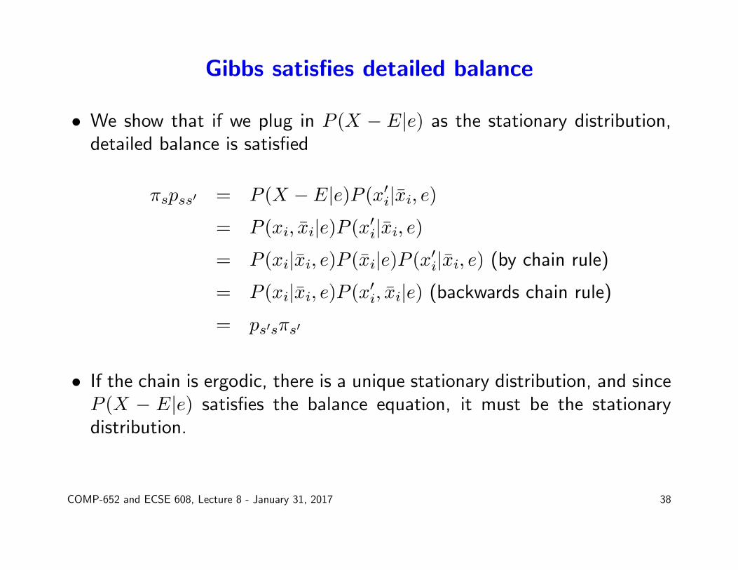
Gibbs satisfies detailed balance
• We show that if we plug in P (X − E|e) as the stationary distribution,detailed balance is satisfied
πspss′ = P (X − E|e)P (x′i|x̄i, e)= P (xi, x̄i|e)P (x′i|x̄i, e)= P (xi|x̄i, e)P (x̄i|e)P (x′i|x̄i, e) (by chain rule)
= P (xi|x̄i, e)P (x′i, x̄i|e) (backwards chain rule)
= ps′sπs′
• If the chain is ergodic, there is a unique stationary distribution, and sinceP (X − E|e) satisfies the balance equation, it must be the stationarydistribution.
COMP-652 and ECSE 608, Lecture 8 - January 31, 2017 38
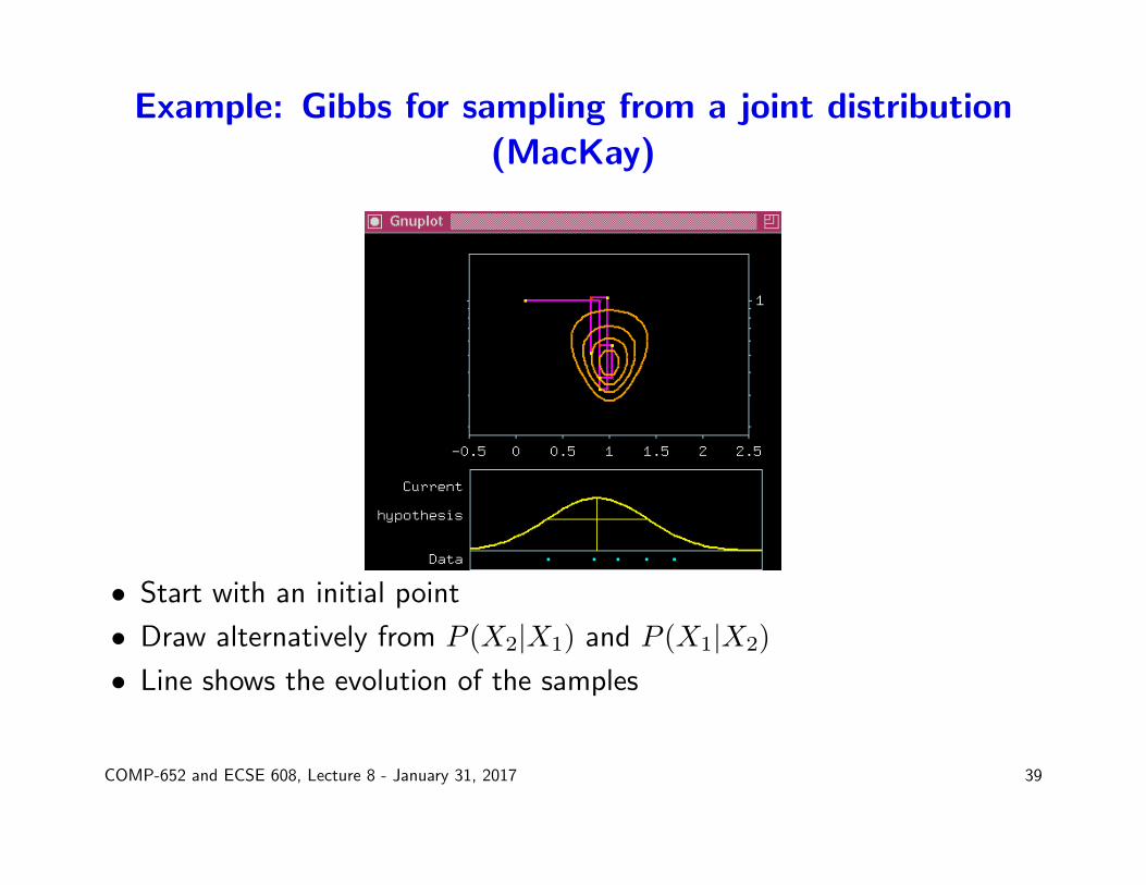
Example: Gibbs for sampling from a joint distribution(MacKay)
• Start with an initial point
• Draw alternatively from P (X2|X1) and P (X1|X2)
• Line shows the evolution of the samples
COMP-652 and ECSE 608, Lecture 8 - January 31, 2017 39

Mixing time
• Gibbs sampling can be viewed as a method for sampling from thestationary distribution of a Markov chain
• This is done by sampling successively from a sequence pt of distributions
• Hence, it is useful to know for what value of t we have pt ≈ π• This is called the mixing time of the chain
• If the mixing time is “small” (e.g. compared to the number of states inthe chain) we say the chain is rapidly mixing
• Unfortunately, the mixing time is hard to estimate (it depends on thegap between the first two eigenvalues of the transition matrix)
• In practice, it is best to wait as long as possible to generate a sample(this is called the burn-in time)
COMP-652 and ECSE 608, Lecture 8 - January 31, 2017 40

Markov Chain Monte Carlo (MCMC) methods
• Suppose you want to generate samples from some distribution, but it ishard to get samples directly
E.g., We want to sample uniformly the space of graphs with certainproperties
• We set up a Markov chain such that its stationary distribution is thedesired distribution
• Note that the ‘states” of this chain can be fairly complicated!
• Start at some state, wait for some number of transitions, then takesamples
• For this to work we need to ensure that:
– the chain has a unique stationary distribution– the stationary distribution is equal to the desired distribution– we reach the stationary distribution quickly
COMP-652 and ECSE 608, Lecture 8 - January 31, 2017 41
Sampling the equilibrium distribution
• We can sample π just by running the chain a long time:
– Set s0 = i for some arbitrary i– For t = 1, . . . ,M , if st = s, sample a value s′ for st+1 based on pss′– Return sM .
If M is large enough, this will be a sample from π
• In practice, we would like to have a rapidly mixing chain, i.e. one thatreaches the equilibrium quickly
COMP-652 and ECSE 608, Lecture 8 - January 31, 2017 42
Example: Random graphs
• Suppose you want to sample uniformly from the space of graphs withv vertices and certain properties (e.g. certain in-degree and out-degreebounds, cycle properties...)
• You set up a chain whose states are graphs with v vertices
• Transitions consist of adding or removing an arc (reversal too, if thegraphs are directed), with a certain probability
• We start with a graph satisfying the desired property.
• The probabilities are devised based on the distribution that we want toreach in the limit.
COMP-652 and ECSE 608, Lecture 8 - January 31, 2017 43
Implementation issues
• The initial samples are influenced by the starting distribution, so theyneed to be thrown away. This is called the burn-in stage
• Because burn-in can take a while, we would like to draw several samplesfrom the same chain
• However, if we take samples t, t+1, t+2..., they will be highly correlated
• Usually we wait for burn-in, then take every nth sample, for some nsufficiently large. This will ensure that the samples are (for all practicalpurposes) uncorrelated
COMP-652 and ECSE 608, Lecture 8 - January 31, 2017 44
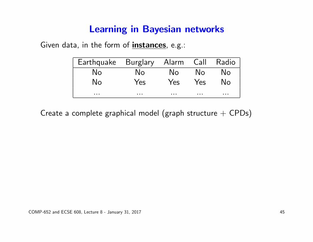
Learning in Bayesian networks
Given data, in the form of instances, e.g.:
Earthquake Burglary Alarm Call RadioNo No No No NoNo Yes Yes Yes No... ... ... ... ...
Create a complete graphical model (graph structure + CPDs)
COMP-652 and ECSE 608, Lecture 8 - January 31, 2017 45

Two learning problems
1. Known vs. unknown structure of the network
I.e. do we know the arcs or do we have to find them too?
2. Complete vs. incomplete data
In real data sets, values for certain variables may be missing, and weneed to “fill in”
Today we focus on the case of known network structure with completedata. This problem is called parameter estimation
COMP-652 and ECSE 608, Lecture 8 - January 31, 2017 46
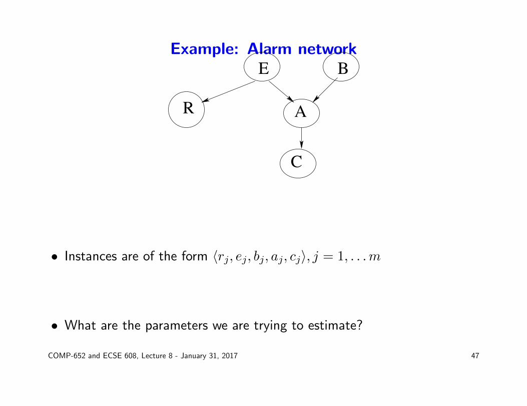
Example: Alarm network
C
E B
R A
• Instances are of the form 〈rj, ej, bj, aj, cj〉, j = 1, . . .m
• What are the parameters we are trying to estimate?
COMP-652 and ECSE 608, Lecture 8 - January 31, 2017 47
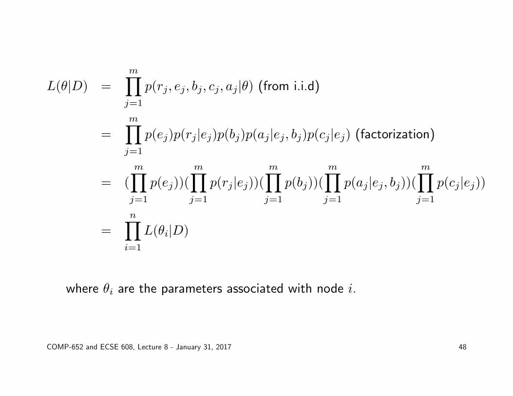
L(θ|D) =
m∏j=1
p(rj, ej, bj, cj, aj|θ) (from i.i.d)
=
m∏j=1
p(ej)p(rj|ej)p(bj)p(aj|ej, bj)p(cj|ej) (factorization)
= (
m∏j=1
p(ej))(
m∏j=1
p(rj|ej))(m∏j=1
p(bj))(
m∏j=1
p(aj|ej, bj))(m∏j=1
p(cj|ej))
=
n∏i=1
L(θi|D)
where θi are the parameters associated with node i.
COMP-652 and ECSE 608, Lecture 8 - January 31, 2017 48

MLE for Bayes nets
Generalizing, for any Bayes net with variables X1, . . . Xn, we have:
L(θ|D) =
m∏j=1
p(x1(j), . . . xn(j)|θ) (from i.i.d)
=
m∏j=1
n∏i=1
p(xi(j)|xπi(j)), θ) (factorization)
=
n∏i=1
m∏j=1
p(xi(j)|xπi(j))
=
n∏i=1
L(θi|D)
The likelihood function decomposes according to the structure of thenetwork, which creates independent estimation problems.
COMP-652 and ECSE 608, Lecture 8 - January 31, 2017 49
Missing data
• Use EM!
• We start with an initial set of parameters
• Use inference to fill in the missing values of all variables
• Re-compute the parameters (which now can be done locally at eachnode)
• These steps are iterated until parameters converge
• Theoretical properties are identical to general EM
COMP-652 and ECSE 608, Lecture 8 - January 31, 2017 50