bayesian nonparametric comorbidity analysis of psychiatric...
TRANSCRIPT
Journal of Machine Learning Research 15 (2014) 1215-1247 Submitted 1/13; Revised 12/13; Published 4/14
Bayesian Nonparametric Comorbidity Analysis ofPsychiatric Disorders
Francisco J. R. Ruiz∗ [email protected] Valera∗ [email protected] of Signal Processing and CommunicationsUniversity Carlos III in MadridAvda. de la Universidad, 3028911 Leganes (Madrid, Spain)
Carlos Blanco [email protected] of Psychiatry, New York State Psychiatric InstituteColumbia University1051 Riverside Drive, Unit #69New York, NY 10032 (United States of America)
Fernando Perez-Cruz [email protected]
Department of Signal Processing and Communications
University Carlos III in Madrid
Avda. de la Universidad, 30
28911 Leganes (Madrid, Spain)
Editor: Athanasios Kottas
Abstract
The analysis of comorbidity is an open and complex research field in the branch of psy-chiatry, where clinical experience and several studies suggest that the relation among thepsychiatric disorders may have etiological and treatment implications. In this paper, weare interested in applying latent feature modeling to find the latent structure behind thepsychiatric disorders that can help to examine and explain the relationships among them.To this end, we use the large amount of information collected in the National EpidemiologicSurvey on Alcohol and Related Conditions (NESARC) database and propose to model thesedata using a nonparametric latent model based on the Indian Buffet Process (IBP). Dueto the discrete nature of the data, we first need to adapt the observation model for discreterandom variables. We propose a generative model in which the observations are drawn froma multinomial-logit distribution given the IBP matrix. The implementation of an efficientGibbs sampler is accomplished using the Laplace approximation, which allows integratingout the weighting factors of the multinomial-logit likelihood model. We also provide avariational inference algorithm for this model, which provides a complementary (and lessexpensive in terms of computational complexity) alternative to the Gibbs sampler allowingus to deal with a larger number of data. Finally, we use the model to analyze comorbidityamong the psychiatric disorders diagnosed by experts from the NESARC database.
Keywords: Bayesian nonparametrics, Indian buffet process, categorical observations,multinomial-logit function, Laplace approximation, variational inference
∗. Both authors contributed equally.
c©2014 Francisco J. R. Ruiz, Isabel Valera, Carlos Blanco and Fernando Perez-Cruz..
Ruiz, Valera, Blanco and Perez-Cruz
1. Introduction
Health care increasingly needs to address the management of individuals with multiplecoexisting diseases, who are now the norm, rather than the exception. In the UnitedStates, about 80% of Medicare spending is devoted to patients with four or more chronicconditions, with costs growing as the number of chronic conditions increases (Wolff et al.,2002). This explains the growing interest of researchers in the impact of comorbidity on arange of outcomes, such as mortality, health-related quality of life, functioning, and qualityof health care. However, attempts to study the impact of comorbidity are complicated bythe lack of consensus about how to define and measure it (Valderas et al., 2009).
Comorbidity becomes particularly relevant in psychiatry, where clinical experience andseveral studies suggest that the relation among the psychiatric disorders may have etiologi-cal and treatment implications. Several studies have focused on the search of the underlyinginterrelationships among psychiatric disorders, which can be useful to analyze the structureof the diagnostic classification system, and guide treatment approaches for each disorder(Blanco et al., 2013). Krueger (1999) found that 10 psychiatric disorders (available inthe National Comorbidity Survey) can be explained by only two correlated factors, onecorresponding to internalizing disorders and the other to externalizing disorders. The exis-tence of the internalizing and the externalizing factors was also confirmed by Kotov et al.(2011). More recently, Blanco et al. (2013) have used factor analysis to find the latent fea-ture structure under 20 common psychiatric disorders, drawing on data from the NationalEpidemiologic Survey on Alcohol and Related Conditions (NESARC). In particular, theauthors found that three correlated factors, one related to externalizing, and the other twoto internalizing disorders, characterized well the underlying structure of these 20 diagnoses.From a statistical point of view, the main limitation of this study lies on the use of factoranalysis, which assumes that the number of factors is known and that the observations areGaussian distributed. However, the latter assumption does not fit the observed data, sincethey are discrete in nature.
In order to avoid the model selection step needed to infer the number of factors infactor analysis, we can resort to Bayesian nonparametric tools, which allow an open-endednumber of degrees of freedom in a model (Jordan, 2010). In this paper, we apply theIndian Buffet Process (IBP) (Griffiths and Ghahramani, 2011), because it allows us to inferwhich latent features influence the observations and how many features there are. Weadapt the observation model for discrete random variables, as the discrete nature of thedata does not allow using the standard Gaussian observation model. There are severaloptions for modeling discrete outputs given the hidden latent features, like a Dirichletdistribution or sampling from the features, but we opted for the generative model partiallyintroduced by Ruiz et al. (2012), in which the observations are drawn from a multinomial-logit distribution, because it resembles the standard Gaussian observation model, as theobservation probability distribution depends on the IBP matrix weighted by some factors.
The IBP model combined with discrete observations has already been tackled in severalrelated works. Williamson et al. (2010) propose a model that combines properties fromboth the hierarchical Dirichlet process (HDP) and the IBP, called IBP compound Dirichlet(ICD) process. They apply the ICD to focused topic modeling, where the instances aredocuments and the observations are words from a finite vocabulary, and focus on decoupling
1216
Bayesian Nonparametric Comorbidity Analysis of Psychiatric Disorders
the prevalence of a topic in a document and its prevalence in all documents. Despite thediscrete nature of the observations under this model, these assumptions are not appropriatefor observations such as the set of possible diagnoses or responses to the questions fromthe NESARC database, since categorical observations can only take values from a finiteset where elements do not present any particular ordering. Titsias (2007) introduced theinfinite gamma-Poisson process as a prior probability distribution over non-negative integervalued matrices with a potentially infinite number of columns, and he applied it to topicmodeling of images. In this model, each (discrete) component in the observation vectorof an instance depends only on one of the active latent features of that object, randomlydrawn from a multinomial distribution. Therefore, different components of the observationvector might be equally distributed. Our model is more flexible in the sense that it allowsdifferent probability distributions for every component in the observation vector, whichis accomplished by weighting differently the latent variables. Furthermore, a preliminaryversion of this model has been successfully applied to identify the factors that model therisk of suicide attempts (Ruiz et al., 2012).
The rest of the paper is organized as follows. In Section 2, we review the IBP modeland the basic Gibbs sampling inference for the IBP, and set the notation used throughoutthe paper. In Section 3, we propose the generative model which combines the IBP withdiscrete observations generated from a multinomial-logit distribution. In this section, wefocus on the inference based on the Gibbs sampler, where we make use of the Laplaceapproximation to integrate out the random weighting factors in the observation model. InSection 4, we develop a variational inference algorithm that presents lower computationalcomplexity than the Gibbs sampler. In Section 5, we validate our model on synthetic dataand apply it over the real data extracted from the NESARC database. Finally, Section 6 isdevoted to the conclusions.
2. The Indian Buffet Process
Unsupervised learning aims to recover the latent structure responsible for generating theobserved properties of a set of objects. In latent feature modeling, the properties of eachobject can be represented by an unobservable vector of latent features, and the observationsare generated from a distribution determined by those latent feature values. Typically, wehave access to the set of observations and the main goal of latent feature modeling is tofind out the latent variables that represent the data.
The most common nonparametric tool for latent feature modeling is the Indian BuffetProcess (IBP). The IBP places a prior distribution over binary matrices, in which thenumber of rows is finite but the number of columns (features) K is potentially unbounded,that is, K → ∞. This distribution is invariant to the ordering of the features and can bederived by taking the limit of a properly defined distribution over N ×K binary matricesas K tends to infinity (Griffiths and Ghahramani, 2011), similarly to the derivation of theChinese restaurant process as the limit of a Dirichlet-multinomial model (Aldous, 1985).However, given a finite number of data points N , it ensures that the number of non-zerocolumns, namely, K+, is finite with probability one.
Let Z be a random N ×K binary matrix distributed following an IBP, i.e., Z ∼ IBP(α),where α is the concentration parameter of the process, which controls the number of non-zero
1217
Ruiz, Valera, Blanco and Perez-Cruz
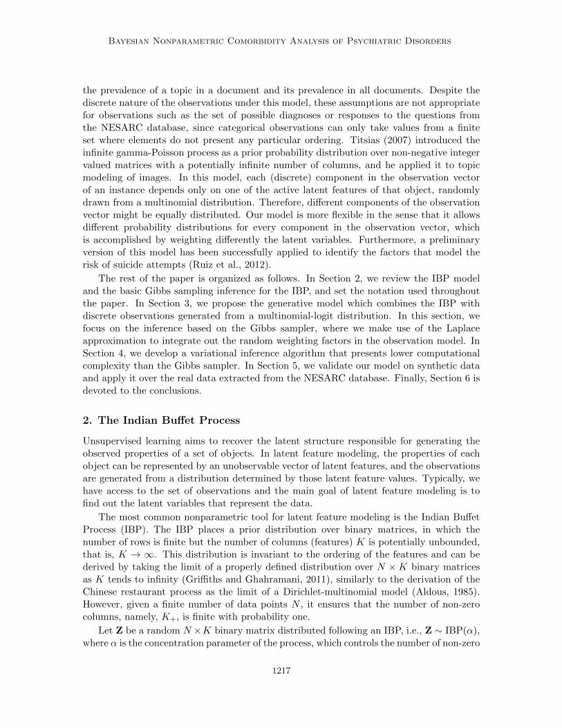
columns K+. The nth row of Z, denoted by zn•, represents the vector of latent features of thenth data point, and every entry nk is denoted by znk. Note that each element znk ∈ {0, 1}indicates whether the kth feature contributes to the nth data point. Since only the K+ non-zero columns of Z contain the features of interest, and due to the exchangeability propertyof the features under the IBP prior, they are usually grouped in the left hand side of thematrix, as illustrated in Figure 1.
Given a binary latent feature matrix Z, we assume that the N×D observation matrix X,where the nth row contains a D-dimensional observation vector xn•, is distributed accordingto a probability distribution p(X|Z). For instance, in the standard observation modelby Griffiths and Ghahramani (2011), p(X|Z) is a Gaussian probability density function.Throughout the paper, we denote by x•d the dth column of X, and the elements in X byxnd.
Z =
26664
z11 z12 · · · z1K+0 0 · · ·
z21 z22 · · · z2K+0 0 · · ·
......
. . ....
......
. . .
zN1 zN2 · · · zNK+0 0 · · ·
37775
K+ non-zero columns
K columns (features)
Ndata
poin
ts
Figure 1: Illustration of an IBP matrix.
2.1 The Stick-Breaking Construction
The stick-breaking construction of the IBP is an equivalent representation of the IBP prior,useful for inference algorithms other than Gibbs sampling, such as slice sampling or varia-tional inference algorithms (Teh et al., 2007; Doshi-Velez et al., 2009).
In this representation, the probability of each latent feature being active is representedexplicitly by a random variable. In particular, the probability of feature znk taking value 1is denoted by ωk, that is,
znk ∼ Bernouilli(ωk).
Since this probability does not depend on n, the stick-breaking representation explicitlyshows that the ordering of the data does not affect the distribution.
The probabilities ωk are, in turn, generated by first drawing a sequence of independentrandom variables v1, v2, . . . from a beta distribution of the form
vk ∼ Beta(α, 1).
Given the sequence of variables v1, v2, . . ., the probability ω1 is assigned to v1, and eachsubsequent ωk is obtained as
ωk =k∏
i=1
vi,
1218
Bayesian Nonparametric Comorbidity Analysis of Psychiatric Disorders
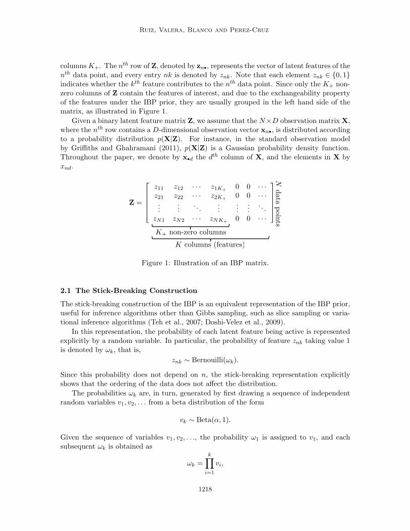
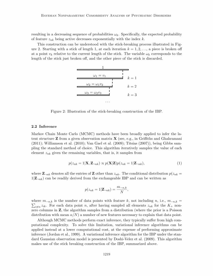
resulting in a decreasing sequence of probabilities ωk. Specifically, the expected probabilityof feature znk being active decreases exponentially with the index k.
This construction can be understood with the stick-breaking process illustrated in Fig-ure 2. Starting with a stick of length 1, at each iteration k = 1, 2, . . ., a piece is broken offat a point vk relative to the current length of the stick. The variable ωk corresponds to thelength of the stick just broken off, and the other piece of the stick is discarded.
1
!1 = v1
!2 = !1v2
!3 = !2v3
. . .
k = 1
k = 2
k = 3
Figure 2: Illustration of the stick-breaking construction of the IBP.
2.2 Inference
Markov Chain Monte Carlo (MCMC) methods have been broadly applied to infer the la-tent structure Z from a given observation matrix X (see, e.g., in Griffiths and Ghahramani(2011); Williamson et al. (2010); Van Gael et al. (2009); Titsias (2007)), being Gibbs sam-pling the standard method of choice. This algorithm iteratively samples the value of eachelement znk given the remaining variables, that is, it samples from
p(znk = 1|X,Z¬nk) ∝ p(X|Z)p(znk = 1|Z¬nk), (1)
where Z¬nk denotes all the entries of Z other than znk. The conditional distribution p(znk =1|Z¬nk) can be readily derived from the exchangeable IBP and can be written as
p(znk = 1|Z¬nk) =m−n,kN
,
where m−n,k is the number of data points with feature k, not including n, i.e., m−n,k =∑i 6=n zik. For each data point n, after having sampled all elements znk for the K+ non-
zero columns in Z, the algorithm samples from a distribution (where the prior is a Poissondistribution with mean α/N) a number of new features necessary to explain that data point.
Although MCMC methods perform exact inference, they typically suffer from high com-putational complexity. To solve this limitation, variational inference algorithms can beapplied instead at a lower computational cost, at the expense of performing approximateinference (Jordan et al., 1999). A variational inference algorithm for the IBP under the stan-dard Gaussian observation model is presented by Doshi-Velez et al. (2009). This algorithmmakes use of the stick breaking construction of the IBP, summarized above.
1219
Ruiz, Valera, Blanco and Perez-Cruz
3. Observation Model
Unlike the standard Gaussian observation model, let us consider discrete observations, thatis, each element xnd ∈ {1, . . . , Rd}, where this finite set contains the indexes to all thepossible values of xnd. For simplicity and without loss of generality, we consider thatRd = R, but the following results can be readily extended to a different cardinality perinput dimension, as well as mixing continuous variables with discrete variables, since giventhe latent feature matrix Z the columns of X are assumed to be independent.
We introduce the K × R matrices Bd and the length-R row vectors bd0 to model the
probability distribution over X, such that Bd links the latent features with the dth columnof the observation matrix X, denoted by x•d, and bd
0 is included to model the bias termin the distribution over the data points. This bias term plays the role of a latent variablethat is always active. For a categorical observation space, if we do not have a bias term andall latent variables are inactive, the model assumes that all the outcomes are independentand equally likely, which is not a suitable assumption in most cases. In our application, thebias term is used to model the people that do not suffer from any disorder and it capturesthe baseline diagnosis in the general population. Additionally, this bias term simplifies theinference since the latent features of those subjects that are not diagnosed any disorder donot need to be sampled.
Hence, we assume that the probability of each element xnd taking value r (r = 1, . . . , R),denoted by πrnd, is given by the multiple-logistic function, i.e.,
πrnd = p(xnd = r|zn•,Bd,bd0) =
exp (zn•bd•r + bd0r)
R∑
r′=1
exp (zn•bd•r′ + bd0r′)
, (2)
where bd•r denotes the rth column of Bd and bd0r denotes the rth element of vector bd
0. Notethat the matrices Bd are used to weight differently the contribution of each latent featureto every component d, similarly as in the standard Gaussian observation model in Griffithsand Ghahramani (2011). We assume that the mixing vectors bd
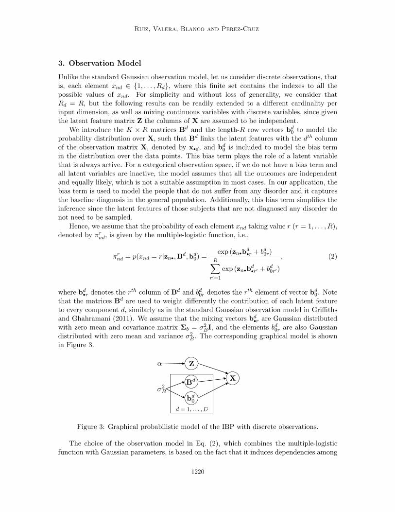
•r are Gaussian distributedwith zero mean and covariance matrix Σb = σ2BI, and the elements bd0r are also Gaussiandistributed with zero mean and variance σ2B. The corresponding graphical model is shownin Figure 3.
Z
XBd
bd0
�2B
d = 1, . . . , D
↵
Figure 3: Graphical probabilistic model of the IBP with discrete observations.
The choice of the observation model in Eq. (2), which combines the multiple-logisticfunction with Gaussian parameters, is based on the fact that it induces dependencies among
1220
Bayesian Nonparametric Comorbidity Analysis of Psychiatric Disorders
the probabilities πrnd that cannot be captured with other distributions, such as the Dirich-let distribution (Blei and Lafferty, 2007). Furthermore, this multinomial-logistic normaldistribution has been widely used to define probability distributions over discrete randomvariables (Williams and Barber, 1998; Blei and Lafferty, 2007).
We consider that elements xnd are independent given the latent feature matrix Z, theweighting matrices Bd and the weighting vectors bd
0. Then, the likelihood for any matrixX can be expressed as
p(X|Z,B1, . . . ,BD,b10, . . . ,b
D0 ) =
N∏
n=1
D∏
d=1
p(xnd|zn•,Bd,bd0) =
N∏
n=1
D∏
d=1
πxndnd . (3)
3.1 Laplace Approximation for Gibbs Sampling Inference
In Section 2, the (heuristic) Gibbs sampling algorithm for posterior inference over the latentvariables of the IBP, detailed in Griffiths and Ghahramani (2011), has been briefly reviewed.To sample from Eq. (1), we need to integrate out Bd and bd
0 in (3), as sequentially samplingfrom the posterior distribution of these variables is intractable, for which an approximationis required. We rely on the Laplace approximation to integrate out the parameters Bd
and bd0 for simplicity and ease of implementation. We first consider the finite form of the
proposed model, where K is bounded.We can simplify the notation in Eqs. 2 and 3 by considering an extended latent feature
matrix Z of size N × (K + 1), in which the elements of the first column are equal to one,and D extended weighting matrices Bd of size (K + 1) × R, in which the first row equalsthe vector bd
0. With these definitions, Eq. (2) can be rewritten as
πrnd = p(xnd = r|zn•,Bd) =exp (zn•b
d•r)
R∑
r′=1
exp (zn•bd•r′)
.
Unless otherwise specified, we use the simplified notation throughout this section. For thisreason, the index k over the latent variables takes the values in {0, 1, . . . ,K}, with zn0 = 1for all n.
Recall that our model assumes independence among the observations given the hiddenlatent variables. Then, the posterior p(B1, . . . ,BD|X,Z) factorizes as
p(B1, . . . ,BD|X,Z) =D∏
d=1
p(Bd|x•d,Z) =D∏
d=1
p(x•d|Bd,Z)p(Bd)
p(x•d|Z).
Hence, we only need to deal with each term p(Bd|x•d,Z) individually. The marginal likeli-hood p(x•d|Z), which we are interested in, can be obtained as
p(x•d|Z) =
∫p(x•d|Bd,Z)p(Bd)dBd. (4)
Although the prior p(Bd) is Gaussian, due to the non-conjugacy with the likelihood term,the computation of this integral, as well as the computation of the posterior p(Bd|x•d,Z),turns out to be intractable.
1221

Ruiz, Valera, Blanco and Perez-Cruz
Following a similar procedure as in Gaussian processes for multiclass classification(Williams and Barber, 1998), we approximate the posterior p(Bd|x•d,Z) as a Gaussiandistribution using Laplace’s method. In order to obtain the parameters of the Gaussiandistribution, we define f(Bd) as the un-normalized log-posterior of p(Bd|x•d,Z), i.e.,
f(Bd) = log p(x•d|Bd,Z) + log p(Bd). (5)
As proven in Appendix A, the function f(Bd) is a strictly concave function of Bd andtherefore it has a unique maximum, which is reached at Bd
MAP, denoted by the subscript‘MAP’ (maximum a posteriori) because it coincides with the mean of the Gaussian distri-bution in the Laplace’s approximation. We resort to Newton’s method to compute Bd
MAP.We stack the columns of Bd into βd, i.e., βd = Bd(:) for avid Matlab users. The
posterior p(Bd|x•d,Z) can be approximated as
p(βd|x•d,Z) ≈ N(βd∣∣∣βd
MAP, (−∇∇f)|βdMAP
),
where βdMAP contains all the columns of Bd
MAP stacked into a vector and ∇∇f is the Hessianof f(βd). Hence, by taking the second-order Taylor series expansion of f(βd) around itsmaximum, the computation of the marginal likelihood in (4) results in a Gaussian integral,whose solution can be expressed as
log p(x•d|Z) ≈ − 1
2σ2Btrace
{(Bd
MAP)>BdMAP
}
− 1
2log
∣∣∣∣∣IR(K+1) + σ2B
N∑
n=1
(diag(πnd)− (πnd)>πnd
)⊗ (z>n•zn•)
∣∣∣∣∣+ log p(x•d|BdMAP,Z),
(6)
where πnd is the vector πnd =[π1nd, π
2nd, . . . , π
Rnd
]evaluated at Bd = Bd
MAP, and diag(πnd)is a diagonal matrix with the values of πnd as its diagonal elements.
Similarly as in Griffiths and Ghahramani (2011), it is straightforward to prove that thelimit of Eq. (6) is well-defined if Z has an unbounded number of columns, that is, as K →∞.The resulting expression for the marginal likelihood p(x•d|Z) can be readily obtained fromEq. (6) by replacing K by K+, Z by the submatrix containing only the non-zero columnsof Z, and Bd
MAP by the submatrix containing the K++1 corresponding rows.
3.2 Speeding Up the Matrix Inversion
In this section, we propose a method that reduces the complexity of computing the inverseof the Hessian for Newton’s method (as well as its determinant) from O(R3K3
+ +NR2K2+)
to O(RK3+ + NR2K2
+), effectively accelerating the inference procedure for large values ofR.
Let us denote with Z the matrix that contains only the K+ + 1 non-zero columns ofthe extended full IBP matrix. The inverse of the Hessian for Newton’s method, as well asits determinant in (6), can be efficiently carried out if we rearrange the inverse of ∇∇f asfollows:
(−∇∇f)−1 =
(D−
N∑
n=1
vnv>n
)−1,
1222
Bayesian Nonparametric Comorbidity Analysis of Psychiatric Disorders
where vn = (πnd)>⊗z>n• and D is a block-diagonal matrix, in which each diagonal submatrixis given by
Dr =1
σ2BIK++1 + Z> diag (πr
•d) Z, (7)
with πr•d =
[πr1d, . . . , π
rNd
]>. Since vnv>n is a rank-one matrix, we can apply the Wood-
bury identity (Woodbury, 1949) N times to invert the matrix −∇∇f , similar to the RLS(Recursive Least Squares) updates (Haykin, 2002). At each iteration n = 1, . . . , N , wecompute
(D(n))−1 =(D(n−1) − vnv>n
)−1= (D(n−1))−1 +
(D(n−1))−1vnv>n (D(n−1))−1
1− v>n (D(n−1))−1vn. (8)
For the first iteration, we define D(0) as the block-diagonal matrix D, whose inversematrix involves computing the R matrix inversions of size (K+ + 1) × (K+ + 1) of thematrices in (7), which can be efficiently solved applying the Matrix Inversion Lemma. AfterN iterations of (8), it turns out that (−∇∇f)−1 = (D(N))−1.
In practice, there is no need to iterate over all observations, since all subjects sharingthe same latent feature vector zn• and observation xnd can be grouped together, thereforerequiring (at most) R2K+ iterations instead of N . In our applications, it provides significantsavings in run-time complexity, since R2K+ � N .
For the determinant in (6), similar recursions can be applied using the Matrix De-terminant Lemma (Harville, 1997), which states that |D + vu>| = (1 + v>Du)|D|, and|D(0)| = ∏R
r=1 |Dr|.
4. Variational Inference
Variational inference provides a complementary (and less expensive in terms of computa-tional complexity) alternative to MCMC methods as a general source of approximationmethods for inference in large-scale statistical models (Jordan et al., 1999). In this section,we adapt the infinite variational approach for the linear-Gaussian model with respect toa full IBP prior introduced by Doshi-Velez et al. (2009) to the model proposed in Sec-tion 3. This approach assumes the (truncated) stick-breaking construction for the IBP inSection 2.1, which bounds the number of columns of the IBP matrix by a finite (but largeenough) value, K. Then, in the truncated stick-breaking process, ωk =
∏ki=1 vi for k ≤ K
and zero otherwise.
The hyperparameters of the model are contained in the set H = {α, σ2B} and, similarly,Ψ = {Z,B1, . . . ,BD,b1
0, . . . ,bD0 , v1, . . . , vK} denotes the set of unobserved variables in the
model. Under the truncated stick-breaking construction for the IBP, the joint probabilitydistribution over all the variables p(Ψ,X|H) can be factorized as
p(Ψ,X|H) =
K∏
k=1
(p(vk|α)
N∏
n=1
p(znk|{vi}ki=1)
)D∏
d=1
(p(bd
0|σ2B)
K∏
k=1
p(bdk•|σ2B)
)
×N∏
n=1
D∏
d=1
p(xnd|zn•,Bd,bd0),
1223
Ruiz, Valera, Blanco and Perez-Cruz
where bdk• is the kth row of matrix Bd.
We approximate p(Ψ|X,H) with the variational distribution q(Ψ) given by
q(Ψ) =K∏
k=1
(q(vk|τk1, τk2)
N∏
n=1
q(znk|νnk)
)K∏
k=0
R∏
r=1
D∏
d=1
q(bdkr|φdkr, (σdkr)2),
where the elements of matrix Bd are denoted by bdkr, and
q(vk|τk1, τk2) = Beta(τk1, τk2),
q(bdkr|φdkr, (σdkr)2) = N (φdkr, (σ
dkr)
2),
q(znk|νnk) = Bernoulli(νnk).
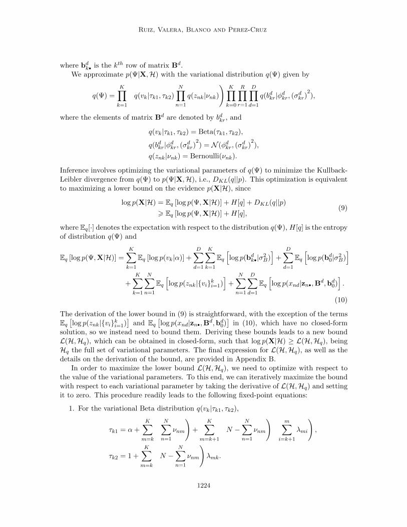
Inference involves optimizing the variational parameters of q(Ψ) to minimize the Kullback-Leibler divergence from q(Ψ) to p(Ψ|X,H), i.e., DKL(q||p). This optimization is equivalentto maximizing a lower bound on the evidence p(X|H), since
log p(X|H) = Eq [log p(Ψ,X|H)] +H[q] +DKL(q||p)> Eq [log p(Ψ,X|H)] +H[q],
(9)
where Eq[·] denotes the expectation with respect to the distribution q(Ψ), H[q] is the entropyof distribution q(Ψ) and
Eq [log p(Ψ,X|H)] =
K∑
k=1
Eq [log p(vk|α)] +
D∑
d=1
K∑
k=1
Eq
[log p(bd
k•|σ2B)]
+
D∑
d=1
Eq
[log p(bd
0|σ2B)]
+
K∑
k=1
N∑
n=1
Eq
[log p(znk|{vi}ki=1)
]+
N∑
n=1
D∑
d=1
Eq
[log p(xnd|zn•,Bd,bd
0)].
(10)
The derivation of the lower bound in (9) is straightforward, with the exception of the termsEq
[log p(znk|{vi}ki=1)
]and Eq
[log p(xnd|zn•,Bd,bd
0)]
in (10), which have no closed-formsolution, so we instead need to bound them. Deriving these bounds leads to a new boundL(H,Hq), which can be obtained in closed-form, such that log p(X|H) ≥ L(H,Hq), beingHq the full set of variational parameters. The final expression for L(H,Hq), as well as thedetails on the derivation of the bound, are provided in Appendix B.
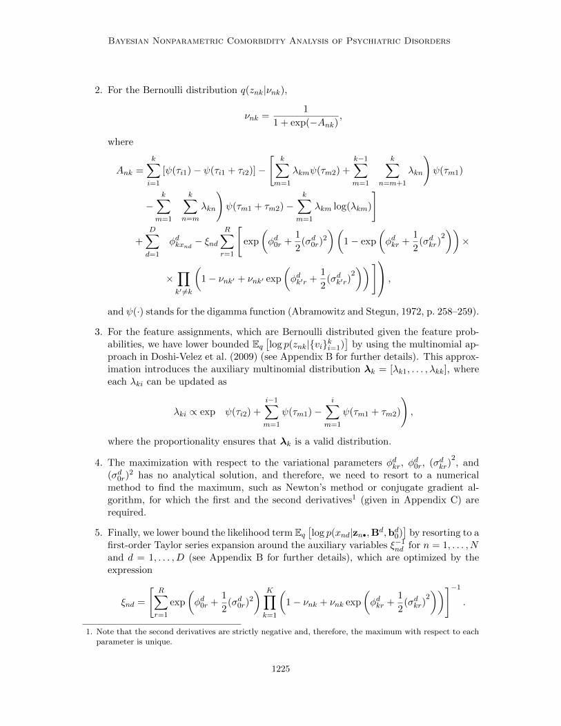
In order to maximize the lower bound L(H,Hq), we need to optimize with respect tothe value of the variational parameters. To this end, we can iteratively maximize the boundwith respect to each variational parameter by taking the derivative of L(H,Hq) and settingit to zero. This procedure readily leads to the following fixed-point equations:
1. For the variational Beta distribution q(vk|τk1, τk2),
τk1 = α+K∑
m=k
(N∑
n=1
νnm
)+
K∑
m=k+1
(N −
N∑
n=1
νnm
)(m∑
i=k+1
λmi
),
τk2 = 1 +K∑
m=k
(N −
N∑
n=1
νnm
)λmk.
1224
Bayesian Nonparametric Comorbidity Analysis of Psychiatric Disorders
2. For the Bernoulli distribution q(znk|νnk),
νnk =1
1 + exp(−Ank),
where
Ank =k∑
i=1
[ψ(τi1)− ψ(τi1 + τi2)]−[
k∑
m=1
λkmψ(τm2) +k−1∑
m=1
(k∑
n=m+1
λkn
)ψ(τm1)
−k∑
m=1
(k∑
n=m
λkn
)ψ(τm1 + τm2)−
k∑
m=1
λkm log(λkm)
]
+D∑
d=1
(φdkxnd
− ξndR∑
r=1
[exp
(φd0r +
1
2(σd0r)
2
)(1− exp
(φdkr +
1
2(σdkr)
2))×
×∏
k′ 6=k
(1− νnk′ + νnk′ exp
(φdk′r +
1
2(σdk′r)
2))]
,
and ψ(·) stands for the digamma function (Abramowitz and Stegun, 1972, p. 258–259).
3. For the feature assignments, which are Bernoulli distributed given the feature prob-abilities, we have lower bounded Eq
[log p(znk|{vi}ki=1)
]by using the multinomial ap-
proach in Doshi-Velez et al. (2009) (see Appendix B for further details). This approx-imation introduces the auxiliary multinomial distribution λk = [λk1, . . . , λkk], whereeach λki can be updated as
λki ∝ exp
(ψ(τi2) +
i−1∑
m=1
ψ(τm1)−i∑
m=1
ψ(τm1 + τm2)
),
where the proportionality ensures that λk is a valid distribution.
4. The maximization with respect to the variational parameters φdkr, φd0r, (σdkr)
2, and
(σd0r)2 has no analytical solution, and therefore, we need to resort to a numerical
method to find the maximum, such as Newton’s method or conjugate gradient al-gorithm, for which the first and the second derivatives1 (given in Appendix C) arerequired.
5. Finally, we lower bound the likelihood term Eq
[log p(xnd|zn•,Bd,bd
0)]
by resorting to afirst-order Taylor series expansion around the auxiliary variables ξ−1nd for n = 1, . . . , Nand d = 1, . . . , D (see Appendix B for further details), which are optimized by theexpression
ξnd =
[R∑
r=1
exp
(φd0r +
1
2(σd0r)
2
) K∏
k=1
(1− νnk + νnk exp
(φdkr +
1
2(σdkr)
2))]−1
.
1. Note that the second derivatives are strictly negative and, therefore, the maximum with respect to eachparameter is unique.
1225
Ruiz, Valera, Blanco and Perez-Cruz
5. Experiments
In this section, we first use a toy example to show how our model with discrete observationsworks and then we turn to two experiments over the NESARC database.
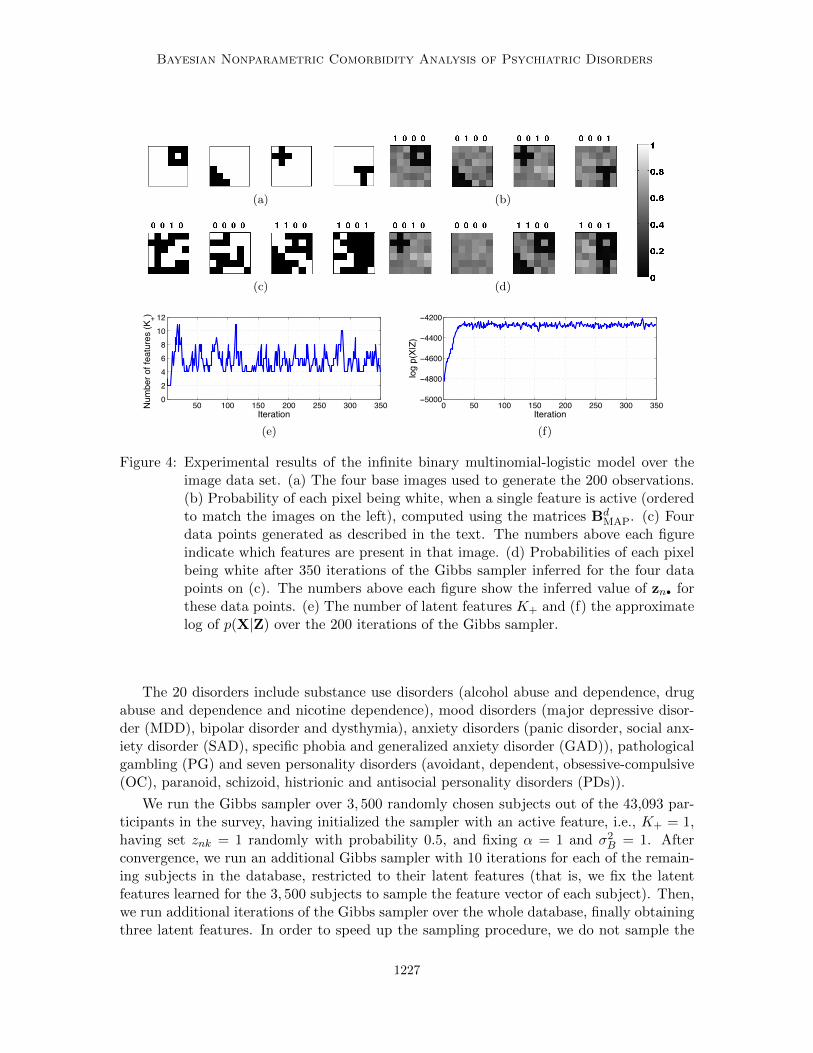
5.1 Inference over Synthetic Images
We generate an illustrative example inspired by the example in Griffiths and Ghahramani(2011) to show that the proposed model works as expected. We define four base black-and-white images, shown in Figure 4a, that can be present with probability 0.3, independentlyof the others. These base images are combined to create a binary composite image. We alsomultiply each white pixel independently with equiprobable binary noise, hence each whitepixel in the composite image can be turned black 50% of the times, while black pixels alwaysremain black. We generate 200 observations to learn the IBP model (several examples canbe found in Figure 4c). The Gibbs sampler has been initialized with K+ = 2, setting eachznk = 1 with probability 1/2, and setting the hyperparameters to α = 0.5 and σ2B = 1.
After 350 iterations, the Gibbs sampler returns four latent features. Each of the fourfeatures recovers one of the base images with a different ordering, which is inconsequential.In Figure 4b, we have plotted the posterior probability for each pixel being white, whenonly one of the components is active. As expected, the black pixels are known to be black(almost zero probability of being white) and the white pixels have about a 50/50 chance ofbeing black or white, due to the multiplicative noise. The Gibbs sampler has used as manyas eleven hidden features, as shown in Figure 4e, but after less than 50 iterations, the firstfour features represent the base images and the others just lock on to a noise pattern, whicheventually fades away.
In Figure 4d, we depict the posterior probability of pixels being white for the fourimages in Figure 4c, given the inferred latent feature vectors for these observations. Notethat the model behaves as expected and properly captures the generative process, even forthose observations which do not possess any latent features, for which the vectors bd
0 donot provide significant information about the black-or-white probabilities.
5.2 Comorbidity Analysis of Psychiatric Disorders
In the present study, our objective is to provide an alternative to the factor analysis approachused by Blanco et al. (2013) with the IBP for discrete observations introduced in the presentpaper. We build an unsupervised model taking the 20 disorders used by Blanco et al. (2013)as input data, drawn from the NESARC data.
The NESARC database was designed to estimate the prevalence of psychiatric disorders,as well as their associated features and level of disability. The NESARC had two wavesof interviews (first wave in 2001-2002 and second wave in 2004-2005). For the followingexperimental results, we only use the data from the first wave, for which 43,093 people wereselected to represent the U.S. population of 18 years of age and older. Through 2,991 entries,the NESARC collects data on the background of participants, alcohol and other drug useand use disorders, and other mental disorders. Public use data are currently available forthis wave of data collection.2
2. See http://aspe.hhs.gov/hsp/06/catalog-ai-an-na/nesarc.htm
1226
Bayesian Nonparametric Comorbidity Analysis of Psychiatric Disorders
(a) (b)
(c) (d)
50 100 150 200 250 300 35002468
1012
Iteration
Num
ber o
f fea
ture
s (K
+)
(e)
0 50 100 150 200 250 300 350−5000
−4800
−4600
−4400
−4200
Iterationlo
g p(
X|Z)
(f)
Figure 4: Experimental results of the infinite binary multinomial-logistic model over theimage data set. (a) The four base images used to generate the 200 observations.(b) Probability of each pixel being white, when a single feature is active (orderedto match the images on the left), computed using the matrices Bd
MAP. (c) Fourdata points generated as described in the text. The numbers above each figureindicate which features are present in that image. (d) Probabilities of each pixelbeing white after 350 iterations of the Gibbs sampler inferred for the four datapoints on (c). The numbers above each figure show the inferred value of zn• forthese data points. (e) The number of latent features K+ and (f) the approximatelog of p(X|Z) over the 200 iterations of the Gibbs sampler.
The 20 disorders include substance use disorders (alcohol abuse and dependence, drugabuse and dependence and nicotine dependence), mood disorders (major depressive disor-der (MDD), bipolar disorder and dysthymia), anxiety disorders (panic disorder, social anx-iety disorder (SAD), specific phobia and generalized anxiety disorder (GAD)), pathologicalgambling (PG) and seven personality disorders (avoidant, dependent, obsessive-compulsive(OC), paranoid, schizoid, histrionic and antisocial personality disorders (PDs)).
We run the Gibbs sampler over 3, 500 randomly chosen subjects out of the 43,093 par-ticipants in the survey, having initialized the sampler with an active feature, i.e., K+ = 1,having set znk = 1 randomly with probability 0.5, and fixing α = 1 and σ2B = 1. Afterconvergence, we run an additional Gibbs sampler with 10 iterations for each of the remain-ing subjects in the database, restricted to their latent features (that is, we fix the latentfeatures learned for the 3, 500 subjects to sample the feature vector of each subject). Then,we run additional iterations of the Gibbs sampler over the whole database, finally obtainingthree latent features. In order to speed up the sampling procedure, we do not sample the
1227
Ruiz, Valera, Blanco and Perez-Cruz
10−4
10−3
10−2
10−1
100P
roba
bilit
y
1. A
lcoh
ol a
buse
2. A
lcoh
ol d
epen
d.3.
Dru
g ab
use
4. D
rug
depe
nd.
5. N
icot
ine
depe
nd.
6. M
DD
7. B
ipol
ar d
isor
der
8. D
ysth
ymia
9. P
anic
dis
orde
r10
. SA
D11
. Spe
cific
pho
bia
12. G
AD
13. P
G14
. Avo
idan
t PD
15. D
epen
dent
PD
16. O
CP
D17
. Par
anoi
d P
D18
. Sch
izoi
d P
D19
. His
trion
ic P
D20
. Ant
isoc
ial P
D
[000][100][010][001]Baseline
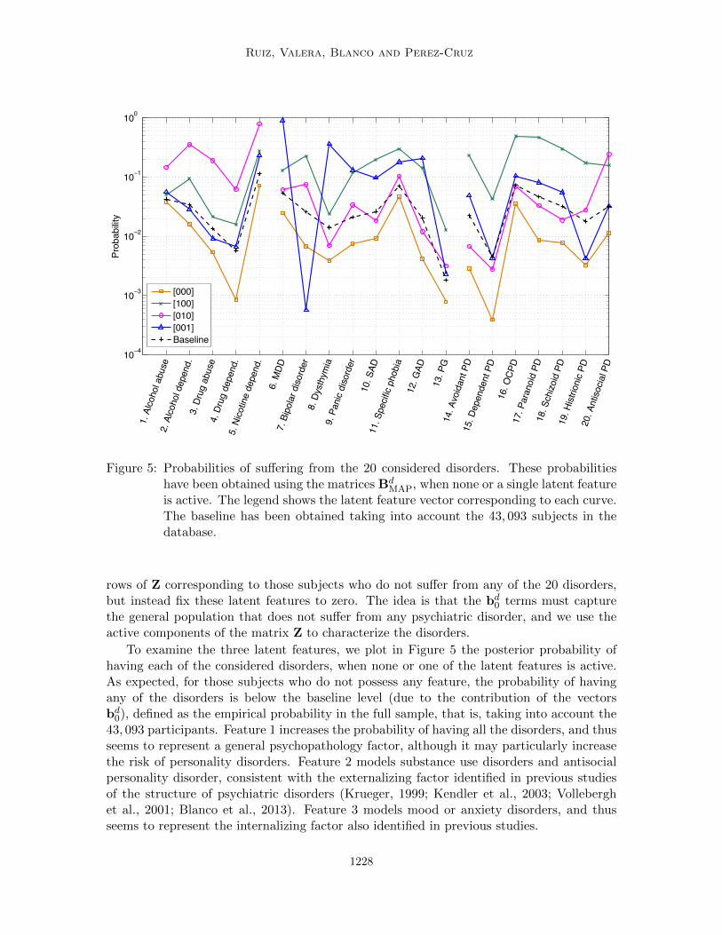
Figure 5: Probabilities of suffering from the 20 considered disorders. These probabilitieshave been obtained using the matrices Bd
MAP, when none or a single latent featureis active. The legend shows the latent feature vector corresponding to each curve.The baseline has been obtained taking into account the 43, 093 subjects in thedatabase.
rows of Z corresponding to those subjects who do not suffer from any of the 20 disorders,but instead fix these latent features to zero. The idea is that the bd
0 terms must capturethe general population that does not suffer from any psychiatric disorder, and we use theactive components of the matrix Z to characterize the disorders.
To examine the three latent features, we plot in Figure 5 the posterior probability ofhaving each of the considered disorders, when none or one of the latent features is active.As expected, for those subjects who do not possess any feature, the probability of havingany of the disorders is below the baseline level (due to the contribution of the vectorsbd0), defined as the empirical probability in the full sample, that is, taking into account the
43, 093 participants. Feature 1 increases the probability of having all the disorders, and thusseems to represent a general psychopathology factor, although it may particularly increasethe risk of personality disorders. Feature 2 models substance use disorders and antisocialpersonality disorder, consistent with the externalizing factor identified in previous studiesof the structure of psychiatric disorders (Krueger, 1999; Kendler et al., 2003; Volleberghet al., 2001; Blanco et al., 2013). Feature 3 models mood or anxiety disorders, and thusseems to represent the internalizing factor also identified in previous studies.
1228
Bayesian Nonparametric Comorbidity Analysis of Psychiatric Disorders
Feature vector 1 x x x 1 x x x 1
Empirical Probability 0.0748 0.0330 0.0227
(a)
Feature vector 1 1 x 1 x 1 x 1 1
Empirical Probability 0.0028 0.0012 0.0009
Product Probability 0.0025 0.0017 0.0007
(b)
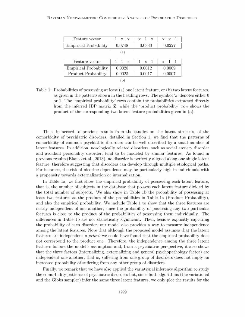
Table 1: Probabilities of possessing at least (a) one latent feature, or (b) two latent features,as given in the patterns shown in the heading rows. The symbol ‘x’ denotes either 0or 1. The ‘empirical probability’ rows contain the probabilities extracted directlyfrom the inferred IBP matrix Z, while the ‘product probability’ row shows theproduct of the corresponding two latent feature probabilities given in (a).
Thus, in accord to previous results from the studies on the latent structure of thecomorbidity of psychiatric disorders, detailed in Section 1, we find that the patterns ofcomorbidity of common psychiatric disorders can be well described by a small number oflatent features. In addition, nosologically related disorders, such as social anxiety disorderand avoidant personality disorder, tend to be modeled by similar features. As found inprevious results (Blanco et al., 2013), no disorder is perfectly aligned along one single latentfeature, therefore suggesting that disorders can develop through multiple etiological paths.For instance, the risk of nicotine dependence may be particularly high in individuals witha propensity towards externalization or internalization.
In Table 1a, we first show the empirical probability of possessing each latent feature,that is, the number of subjects in the database that possess each latent feature divided bythe total number of subjects. We also show in Table 1b the probability of possessing atleast two features as the product of the probabilities in Table 1a (Product Probability),and also the empirical probability. We include Table 1 to show that the three features arenearly independent of one another, since the probability of possessing any two particularfeatures is close to the product of the probabilities of possessing them individually. Thedifferences in Table 1b are not statistically significant. Then, besides explicitly capturingthe probability of each disorder, our model also provides a way to measure independenceamong the latent features. Note that although the proposed model assumes that the latentfeatures are independent a priori, we could have found that the empirical probability doesnot correspond to the product one. Therefore, the independence among the three latentfeatures follows the model’s assumption and, from a psychiatric perspective, it also showsthat the three factors (internalizing, externalizing and general psychopathology factor) areindependent one another, that is, suffering from one group of disorders does not imply anincreased probability of suffering from any other group of disorders.
Finally, we remark that we have also applied the variational inference algorithm to studythe comorbidity patterns of psychiatric disorders but, since both algorithms (the variationaland the Gibbs sampler) infer the same three latent features, we only plot the results for the
1229
Ruiz, Valera, Blanco and Perez-Cruz
Gibbs sampling algorithm in this section and apply the variational inference algorithm innext section.
5.3 Comorbidity Analysis of Personality Disorders
In order to identify the seven personality disorders studied in the previous section, psy-chiatrists have established specific diagnostic criteria for each of them. These criteria cor-respond to affirmative responses to one or several questions in the NESARC survey andthis correspondence is shown in Appendix D. Then, there exists a set of criteria to iden-tify if a subject presents any of the following personality disorders: avoidant, dependent,obsessive-compulsive, paranoid, schizoid, histrionic and antisocial. In the present analysis,we consider as input data the fulfillment of the 52 criteria (i.e., R = 2) corresponding toall the disorders for the 43,093 subjects and we apply the variational inference algorithmtruncated to K = 25 features, as detailed in Section 4, to find the latent structure of thedata.
In order to properly initialize the huge amount of variational parameters, we have pre-viously run six Gibbs samplers over the data but taking only the criteria corresponding tothe avoidant PD and another PD (that is, the seven criteria for the avoidant PD and theseven for the dependent PD, the criteria for the avoidant PD with the eight for the OCPD,etc.) for 10, 000 randomly chosen subjects. After running the six Gibbs samplers, we ob-tain 18 latent features that we group in a unique matrix Z to obtain the weighting matricesBd
MAP, which are used to initialize some parameters νnk and φdkr. We do this because thevariational algorithm is sensitive to the starting point and a random initialization wouldnot produce good solutions.
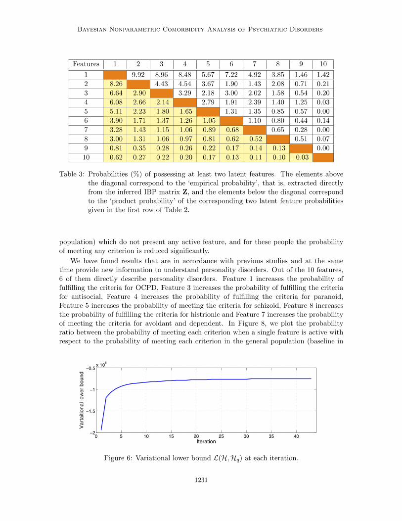
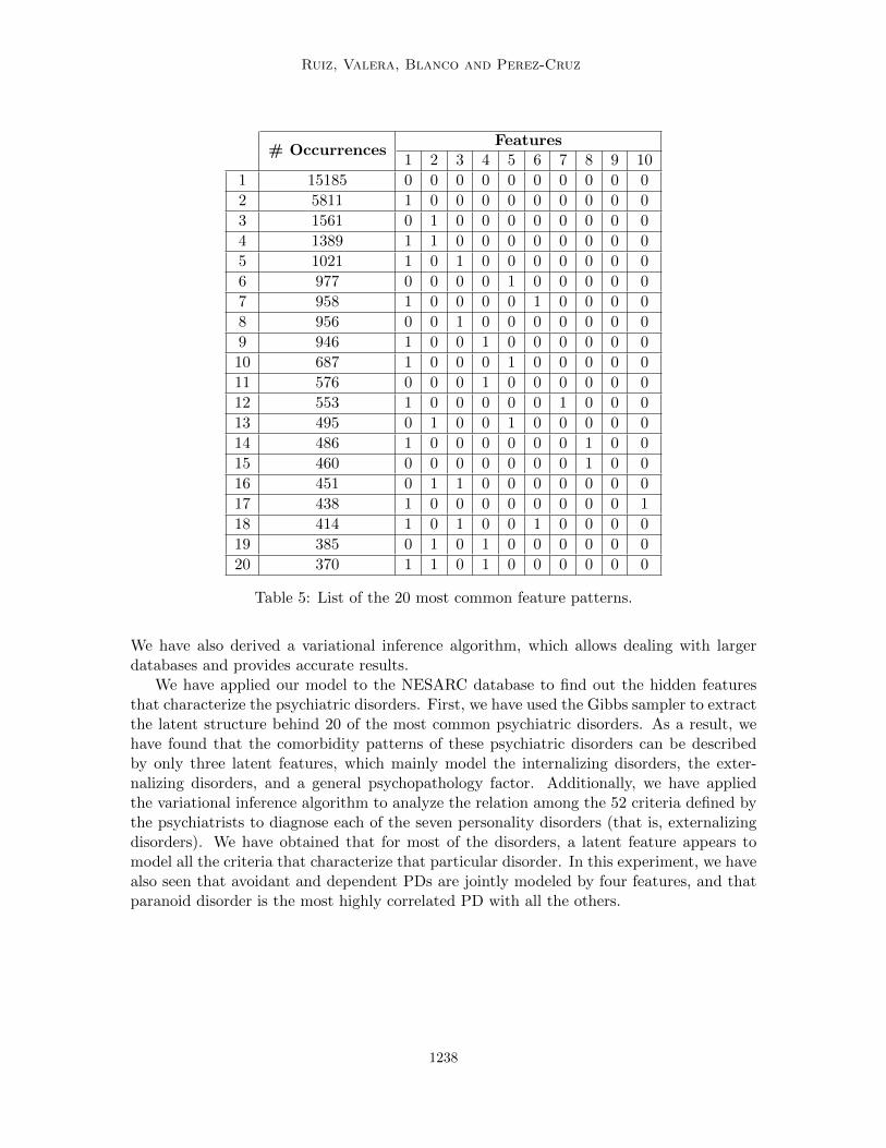
We run enough iterations of the variational algorithm to ensure convergence of thevariational lower bound (the lower bound at each iteration is shown in Figure 6). Weconstruct a binary matrix Z by setting each element znk = 1 if νnk > 0.5. We flip (changingzeros by ones, and vice versa) those features possessed by more than 80% of the subjects,obtaining only 10 latent features possessed by more than 50 subjects among the 43, 093in the database and then recomputing the weighting matrices. In Table 2, we show theprobability of occurrence of each feature (top row), as well as the probability of havingactive only one single feature (bottom row). We also show the ‘empirical’ and the ‘product’probabilities of possessing at least two latent features in Table 3, and the probabilities ofpossessing at least two features given that one of them is active in Table 4.
Features 1 2 3 4 5 6 7 8 9 10
Total 43.45 19.01 15.28 13.99 11.76 8.97 7.54 6.91 1.86 1.43
Single feature 13.48 3.62 2.22 1.34 2.27 0.49 0.76 1.07 0 0
Table 2: Probabilities (%) of possessing (top row) at least one latent feature, or (bottomrow) a single feature.
In Figure 7, we plot the probability of meeting each criterion in the general population(dashed line) and the probability of meeting each criterion for those subjects that do nothave any active feature in our model (solid line). There are 15, 185 subjects (35.2% of the
1230
Bayesian Nonparametric Comorbidity Analysis of Psychiatric Disorders
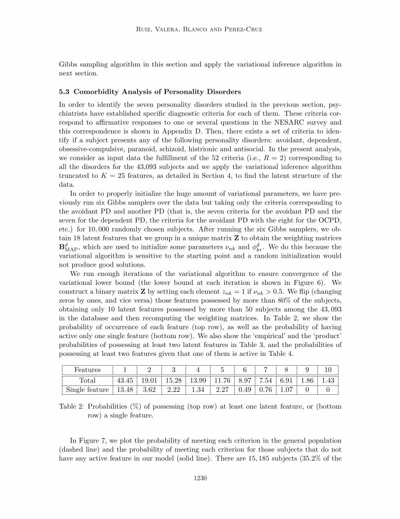
Features 1 2 3 4 5 6 7 8 9 10
1 9.92 8.96 8.48 5.67 7.22 4.92 3.85 1.46 1.42
2 8.26 4.43 4.54 3.67 1.90 1.43 2.08 0.71 0.21
3 6.64 2.90 3.29 2.18 3.00 2.02 1.58 0.54 0.20
4 6.08 2.66 2.14 2.79 1.91 2.39 1.40 1.25 0.03
5 5.11 2.23 1.80 1.65 1.31 1.35 0.85 0.57 0.00
6 3.90 1.71 1.37 1.26 1.05 1.10 0.80 0.44 0.14
7 3.28 1.43 1.15 1.06 0.89 0.68 0.65 0.28 0.00
8 3.00 1.31 1.06 0.97 0.81 0.62 0.52 0.51 0.07
9 0.81 0.35 0.28 0.26 0.22 0.17 0.14 0.13 0.00
10 0.62 0.27 0.22 0.20 0.17 0.13 0.11 0.10 0.03
Table 3: Probabilities (%) of possessing at least two latent features. The elements abovethe diagonal correspond to the ‘empirical probability’, that is, extracted directlyfrom the inferred IBP matrix Z, and the elements below the diagonal correspondto the ‘product probability’ of the corresponding two latent feature probabilitiesgiven in the first row of Table 2.
population) which do not present any active feature, and for these people the probabilityof meeting any criterion is reduced significantly.
We have found results that are in accordance with previous studies and at the sametime provide new information to understand personality disorders. Out of the 10 features,6 of them directly describe personality disorders. Feature 1 increases the probability offulfilling the criteria for OCPD, Feature 3 increases the probability of fulfilling the criteriafor antisocial, Feature 4 increases the probability of fulfilling the criteria for paranoid,Feature 5 increases the probability of meeting the criteria for schizoid, Feature 8 increasesthe probability of fulfilling the criteria for histrionic and Feature 7 increases the probabilityof meeting the criteria for avoidant and dependent. In Figure 8, we plot the probabilityratio between the probability of meeting each criterion when a single feature is active withrespect to the probability of meeting each criterion in the general population (baseline in
0 5 10 15 20 25 30 35 40−2
−1.5
−1
−0.5 x 10⁶
Iteration
Varta
ition
al lo
wer
bou
nd
Figure 6: Variational lower bound L(H,Hq) at each iteration.
1231
Ruiz, Valera, Blanco and Perez-Cruz
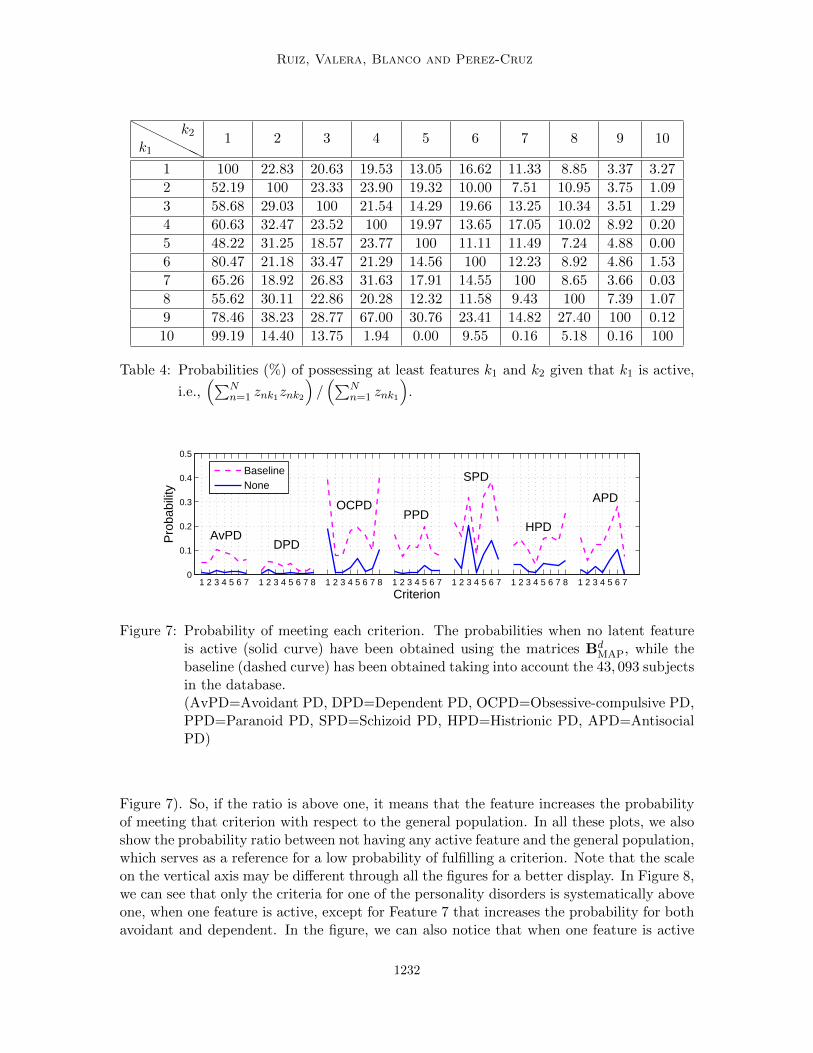
HHHHHHk1
k2 1 2 3 4 5 6 7 8 9 10
1 100 22.83 20.63 19.53 13.05 16.62 11.33 8.85 3.37 3.27
2 52.19 100 23.33 23.90 19.32 10.00 7.51 10.95 3.75 1.09
3 58.68 29.03 100 21.54 14.29 19.66 13.25 10.34 3.51 1.29
4 60.63 32.47 23.52 100 19.97 13.65 17.05 10.02 8.92 0.20
5 48.22 31.25 18.57 23.77 100 11.11 11.49 7.24 4.88 0.00
6 80.47 21.18 33.47 21.29 14.56 100 12.23 8.92 4.86 1.53
7 65.26 18.92 26.83 31.63 17.91 14.55 100 8.65 3.66 0.03
8 55.62 30.11 22.86 20.28 12.32 11.58 9.43 100 7.39 1.07
9 78.46 38.23 28.77 67.00 30.76 23.41 14.82 27.40 100 0.12
10 99.19 14.40 13.75 1.94 0.00 9.55 0.16 5.18 0.16 100
Table 4: Probabilities (%) of possessing at least features k1 and k2 given that k1 is active,
i.e.,(∑N
n=1 znk1znk2
)/(∑N
n=1 znk1
).
1 2 3 4 5 6 7 1 2 3 4 5 6 7 8 1 2 3 4 5 6 7 8 1 2 3 4 5 6 7 1 2 3 4 5 6 7 1 2 3 4 5 6 7 8 1 2 3 4 5 6 70
0.1
0.2
0.3
0.4
0.5
Criterion
Pro
babi
lity
BaselineNone
HPDAvPD
DPD
PPD
SPD
APDOCPD
Figure 7: Probability of meeting each criterion. The probabilities when no latent featureis active (solid curve) have been obtained using the matrices Bd
MAP, while thebaseline (dashed curve) has been obtained taking into account the 43, 093 subjectsin the database.(AvPD=Avoidant PD, DPD=Dependent PD, OCPD=Obsessive-compulsive PD,PPD=Paranoid PD, SPD=Schizoid PD, HPD=Histrionic PD, APD=AntisocialPD)
Figure 7). So, if the ratio is above one, it means that the feature increases the probabilityof meeting that criterion with respect to the general population. In all these plots, we alsoshow the probability ratio between not having any active feature and the general population,which serves as a reference for a low probability of fulfilling a criterion. Note that the scaleon the vertical axis may be different through all the figures for a better display. In Figure 8,we can see that only the criteria for one of the personality disorders is systematically aboveone, when one feature is active, except for Feature 7 that increases the probability for bothavoidant and dependent. In the figure, we can also notice that when one feature is active
1232
Bayesian Nonparametric Comorbidity Analysis of Psychiatric Disorders
1 2 3 4 5 6 7 1 2 3 4 5 6 7 8 1 2 3 4 5 6 7 8 1 2 3 4 5 6 7 1 2 3 4 5 6 7 1 2 3 4 5 6 7 8 1 2 3 4 5 6 70
0.5
1
1.5
2
Criterion
Pro
b. R
atio
NoneF1F4
AvPD
PPD
SPDOCPD
APD
HPDDPD
1 2 3 4 5 6 7 1 2 3 4 5 6 7 8 1 2 3 4 5 6 7 8 1 2 3 4 5 6 7 1 2 3 4 5 6 7 1 2 3 4 5 6 7 8 1 2 3 4 5 6 70
1
2
3
4
5
Criterion
Pro
b. R
atio
NoneF3F8
DPDAvPD OCPD PPD SPD
HPD
APD
1 2 3 4 5 6 7 1 2 3 4 5 6 7 8 1 2 3 4 5 6 7 8 1 2 3 4 5 6 7 1 2 3 4 5 6 7 1 2 3 4 5 6 7 8 1 2 3 4 5 6 70
1
2
3
4
Criterion
Pro
b. R
atio
NoneF5F7
HPD
APD
SPD
OCPDPPD
AvPD
DPD
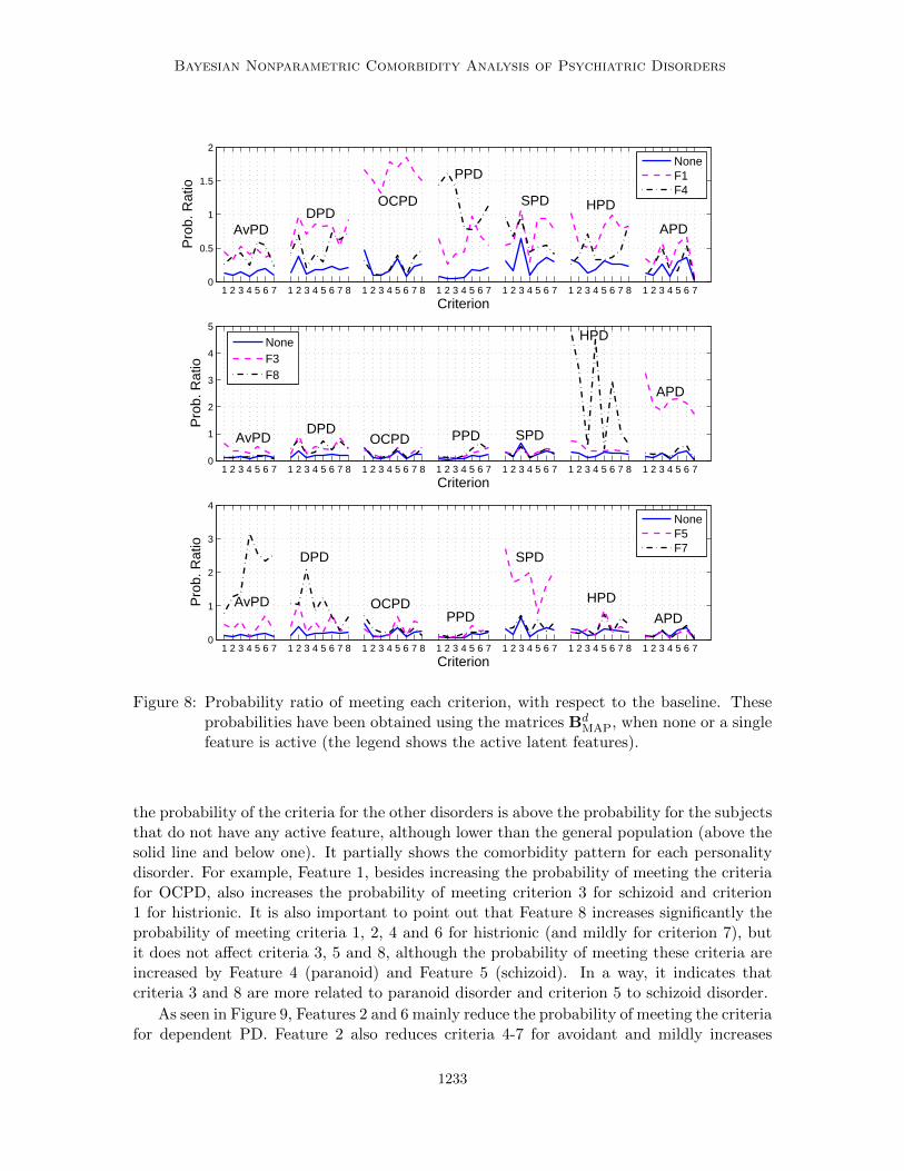
Figure 8: Probability ratio of meeting each criterion, with respect to the baseline. Theseprobabilities have been obtained using the matrices Bd
MAP, when none or a singlefeature is active (the legend shows the active latent features).
the probability of the criteria for the other disorders is above the probability for the subjectsthat do not have any active feature, although lower than the general population (above thesolid line and below one). It partially shows the comorbidity pattern for each personalitydisorder. For example, Feature 1, besides increasing the probability of meeting the criteriafor OCPD, also increases the probability of meeting criterion 3 for schizoid and criterion1 for histrionic. It is also important to point out that Feature 8 increases significantly theprobability of meeting criteria 1, 2, 4 and 6 for histrionic (and mildly for criterion 7), butit does not affect criteria 3, 5 and 8, although the probability of meeting these criteria areincreased by Feature 4 (paranoid) and Feature 5 (schizoid). In a way, it indicates thatcriteria 3 and 8 are more related to paranoid disorder and criterion 5 to schizoid disorder.
As seen in Figure 9, Features 2 and 6 mainly reduce the probability of meeting the criteriafor dependent PD. Feature 2 also reduces criteria 4-7 for avoidant and mildly increases
1233
Ruiz, Valera, Blanco and Perez-Cruz
1 2 3 4 5 6 7 1 2 3 4 5 6 7 8 1 2 3 4 5 6 7 8 1 2 3 4 5 6 7 1 2 3 4 5 6 7 1 2 3 4 5 6 7 8 1 2 3 4 5 6 70
0.5
1
1.5
Criterion
Pro
b. R
atio
NoneF2F6AvPD
DPD
HPD
APD
OCPD PPD
SPD
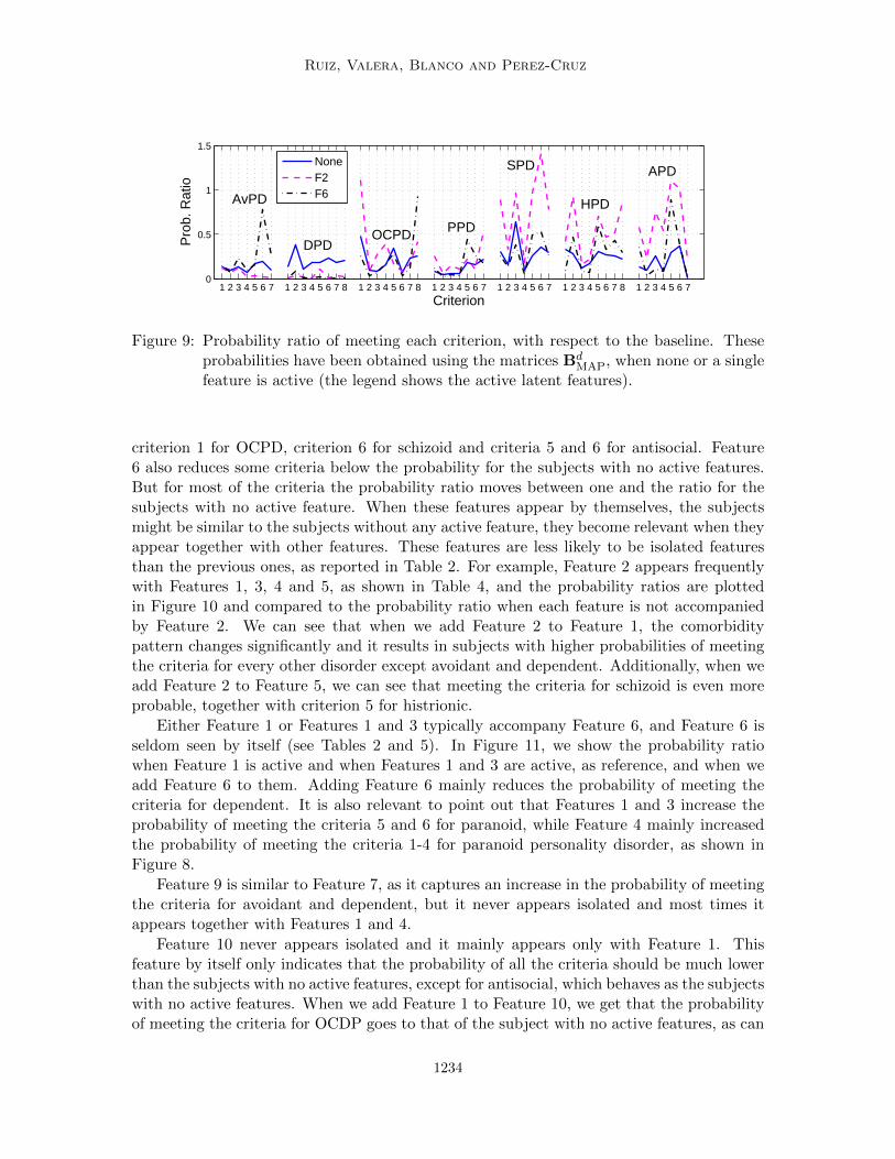
Figure 9: Probability ratio of meeting each criterion, with respect to the baseline. Theseprobabilities have been obtained using the matrices Bd
MAP, when none or a singlefeature is active (the legend shows the active latent features).
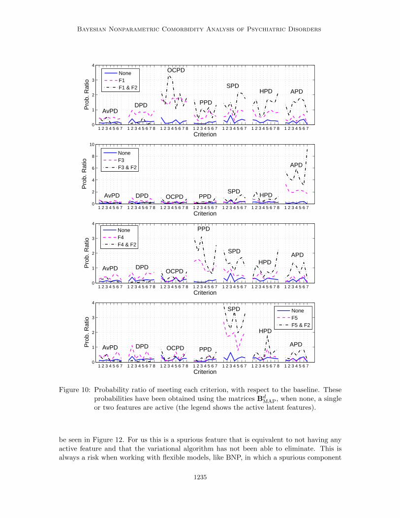
criterion 1 for OCPD, criterion 6 for schizoid and criteria 5 and 6 for antisocial. Feature6 also reduces some criteria below the probability for the subjects with no active features.But for most of the criteria the probability ratio moves between one and the ratio for thesubjects with no active feature. When these features appear by themselves, the subjectsmight be similar to the subjects without any active feature, they become relevant when theyappear together with other features. These features are less likely to be isolated featuresthan the previous ones, as reported in Table 2. For example, Feature 2 appears frequentlywith Features 1, 3, 4 and 5, as shown in Table 4, and the probability ratios are plottedin Figure 10 and compared to the probability ratio when each feature is not accompaniedby Feature 2. We can see that when we add Feature 2 to Feature 1, the comorbiditypattern changes significantly and it results in subjects with higher probabilities of meetingthe criteria for every other disorder except avoidant and dependent. Additionally, when weadd Feature 2 to Feature 5, we can see that meeting the criteria for schizoid is even moreprobable, together with criterion 5 for histrionic.
Either Feature 1 or Features 1 and 3 typically accompany Feature 6, and Feature 6 isseldom seen by itself (see Tables 2 and 5). In Figure 11, we show the probability ratiowhen Feature 1 is active and when Features 1 and 3 are active, as reference, and when weadd Feature 6 to them. Adding Feature 6 mainly reduces the probability of meeting thecriteria for dependent. It is also relevant to point out that Features 1 and 3 increase theprobability of meeting the criteria 5 and 6 for paranoid, while Feature 4 mainly increasedthe probability of meeting the criteria 1-4 for paranoid personality disorder, as shown inFigure 8.
Feature 9 is similar to Feature 7, as it captures an increase in the probability of meetingthe criteria for avoidant and dependent, but it never appears isolated and most times itappears together with Features 1 and 4.
Feature 10 never appears isolated and it mainly appears only with Feature 1. Thisfeature by itself only indicates that the probability of all the criteria should be much lowerthan the subjects with no active features, except for antisocial, which behaves as the subjectswith no active features. When we add Feature 1 to Feature 10, we get that the probabilityof meeting the criteria for OCDP goes to that of the subject with no active features, as can
1234
Bayesian Nonparametric Comorbidity Analysis of Psychiatric Disorders
1 2 3 4 5 6 7 1 2 3 4 5 6 7 8 1 2 3 4 5 6 7 8 1 2 3 4 5 6 7 1 2 3 4 5 6 7 1 2 3 4 5 6 7 8 1 2 3 4 5 6 70
1
2
3
4
Criterion
Pro
b. R
atio
NoneF1F1 & F2
HPD
OCPD
SPDAPD
AvPDDPD PPD
1 2 3 4 5 6 7 1 2 3 4 5 6 7 8 1 2 3 4 5 6 7 8 1 2 3 4 5 6 7 1 2 3 4 5 6 7 1 2 3 4 5 6 7 8 1 2 3 4 5 6 70
2
4
6
8
10
Criterion
Pro
b. R
atio
NoneF3F3 & F2 APD
AvPD DPD OCPDSPD
PPD HPD
1 2 3 4 5 6 7 1 2 3 4 5 6 7 8 1 2 3 4 5 6 7 8 1 2 3 4 5 6 7 1 2 3 4 5 6 7 1 2 3 4 5 6 7 8 1 2 3 4 5 6 70
1
2
3
4
Criterion
Pro
b. R
atio
NoneF4F4 & F2
AvPD DPDOCPD
PPD
SPD
HPDAPD
1 2 3 4 5 6 7 1 2 3 4 5 6 7 8 1 2 3 4 5 6 7 8 1 2 3 4 5 6 7 1 2 3 4 5 6 7 1 2 3 4 5 6 7 8 1 2 3 4 5 6 70
1
2
3
4
Criterion
Pro
b. R
atio
NoneF5F5 & F2
AvPD DPD PPDOCPDAPD
HPD
SPD
Figure 10: Probability ratio of meeting each criterion, with respect to the baseline. Theseprobabilities have been obtained using the matrices Bd
MAP, when none, a singleor two features are active (the legend shows the active latent features).
be seen in Figure 12. For us this is a spurious feature that is equivalent to not having anyactive feature and that the variational algorithm has not been able to eliminate. This isalways a risk when working with flexible models, like BNP, in which a spurious component
1235
Ruiz, Valera, Blanco and Perez-Cruz
1 2 3 4 5 6 7 1 2 3 4 5 6 7 8 1 2 3 4 5 6 7 8 1 2 3 4 5 6 7 1 2 3 4 5 6 7 1 2 3 4 5 6 7 8 1 2 3 4 5 6 70
0.5
1
1.5
2
2.5
Criterion
Pro
b. R
atio
NoneF1F1 & F6
AvPD DPD
PPD
SPD HPD APDOCPD
1 2 3 4 5 6 7 1 2 3 4 5 6 7 8 1 2 3 4 5 6 7 8 1 2 3 4 5 6 7 1 2 3 4 5 6 7 1 2 3 4 5 6 7 8 1 2 3 4 5 6 70
1
2
3
4
5
6
Criterion
Pro
b. R
atio
NoneF1 & F3F1, F3 & F6
DPD OCPD PPDAvPD SPD HPD
APD
Figure 11: Probability ratio of meeting each criterion, with respect to the baseline. Theseprobabilities have been obtained using the matrices Bd
MAP, when none, a singleor several features are active (the legend shows the active latent features).
1 2 3 4 5 6 7 1 2 3 4 5 6 7 8 1 2 3 4 5 6 7 8 1 2 3 4 5 6 7 1 2 3 4 5 6 7 1 2 3 4 5 6 7 8 1 2 3 4 5 6 70
0.2
0.4
0.6
0.8
1
Criterion
Pro
b. R
atio
NoneF1 & F10F10
OCPDDPDAvPD
HPD
SPD
PPD
APD
Figure 12: Probability ratio of meeting each criterion, with respect to the baseline. Theseprobabilities have been obtained using the matrices Bd
MAP, when none, a singleor two features are active (the legend shows the active latent features).
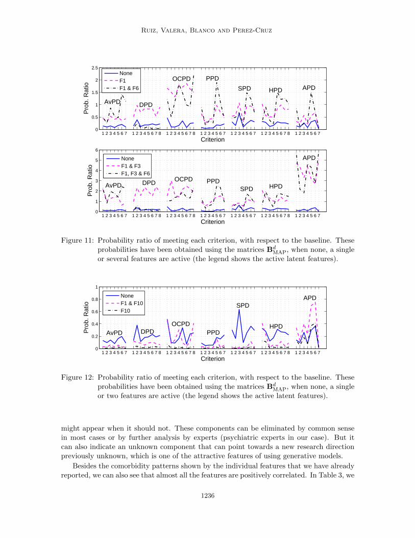
might appear when it should not. These components can be eliminated by common sensein most cases or by further analysis by experts (psychiatric experts in our case). But itcan also indicate an unknown component that can point towards a new research directionpreviously unknown, which is one of the attractive features of using generative models.
Besides the comorbidity patterns shown by the individual features that we have alreadyreported, we can also see that almost all the features are positively correlated. In Table 3, we
1236
Bayesian Nonparametric Comorbidity Analysis of Psychiatric Disorders
1 2 3 4 5 6 7 1 2 3 4 5 6 7 8 1 2 3 4 5 6 7 8 1 2 3 4 5 6 7 1 2 3 4 5 6 7 1 2 3 4 5 6 7 8 1 2 3 4 5 6 70
2
4
6
8
10
12
Criterion
Pro
b. R
atio
NoneF4F4 & F7
OCPD APDHPDSPD
PPDDPD
AvPD
1 2 3 4 5 6 7 1 2 3 4 5 6 7 8 1 2 3 4 5 6 7 8 1 2 3 4 5 6 7 1 2 3 4 5 6 7 1 2 3 4 5 6 7 8 1 2 3 4 5 6 70
2
4
6
8
10
12
Criterion
Pro
b. R
atio
NoneF4F4 & F9
SPDOCPD
AvPDDPD
PPD
HPD
APD
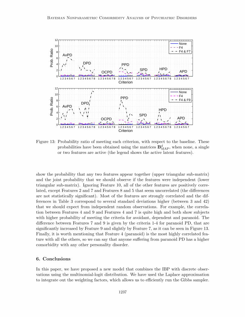
Figure 13: Probability ratio of meeting each criterion, with respect to the baseline. Theseprobabilities have been obtained using the matrices Bd
MAP, when none, a singleor two features are active (the legend shows the active latent features).
show the probability that any two features appear together (upper triangular sub-matrix)and the joint probability that we should observe if the features were independent (lowertriangular sub-matrix). Ignoring Feature 10, all of the other features are positively corre-lated, except Features 2 and 7 and Features 8 and 5 that seem uncorrelated (the differencesare not statistically significant). Most of the features are strongly correlated and the dif-ferences in Table 3 correspond to several standard deviations higher (between 3 and 42)that we should expect from independent random observations. For example, the correla-tion between Features 4 and 9 and Features 4 and 7 is quite high and both show subjectswith higher probability of meeting the criteria for avoidant, dependent and paranoid. Thedifference between Features 7 and 9 is given by the criteria 1-4 for paranoid PD, that aresignificantly increased by Feature 9 and slightly by Feature 7, as it can be seen in Figure 13.Finally, it is worth mentioning that Feature 4 (paranoid) is the most highly correlated fea-ture with all the others, so we can say that anyone suffering from paranoid PD has a highercomorbidity with any other personality disorder.
6. Conclusions
In this paper, we have proposed a new model that combines the IBP with discrete obser-vations using the multinomial-logit distribution. We have used the Laplace approximationto integrate out the weighting factors, which allows us to efficiently run the Gibbs sampler.
1237
Ruiz, Valera, Blanco and Perez-Cruz
# OccurrencesFeatures
1 2 3 4 5 6 7 8 9 10
1 15185 0 0 0 0 0 0 0 0 0 0
2 5811 1 0 0 0 0 0 0 0 0 0
3 1561 0 1 0 0 0 0 0 0 0 0
4 1389 1 1 0 0 0 0 0 0 0 0
5 1021 1 0 1 0 0 0 0 0 0 0
6 977 0 0 0 0 1 0 0 0 0 0
7 958 1 0 0 0 0 1 0 0 0 0
8 956 0 0 1 0 0 0 0 0 0 0
9 946 1 0 0 1 0 0 0 0 0 0
10 687 1 0 0 0 1 0 0 0 0 0
11 576 0 0 0 1 0 0 0 0 0 0
12 553 1 0 0 0 0 0 1 0 0 0
13 495 0 1 0 0 1 0 0 0 0 0
14 486 1 0 0 0 0 0 0 1 0 0
15 460 0 0 0 0 0 0 0 1 0 0
16 451 0 1 1 0 0 0 0 0 0 0
17 438 1 0 0 0 0 0 0 0 0 1
18 414 1 0 1 0 0 1 0 0 0 0
19 385 0 1 0 1 0 0 0 0 0 0
20 370 1 1 0 1 0 0 0 0 0 0
Table 5: List of the 20 most common feature patterns.
We have also derived a variational inference algorithm, which allows dealing with largerdatabases and provides accurate results.
We have applied our model to the NESARC database to find out the hidden featuresthat characterize the psychiatric disorders. First, we have used the Gibbs sampler to extractthe latent structure behind 20 of the most common psychiatric disorders. As a result, wehave found that the comorbidity patterns of these psychiatric disorders can be describedby only three latent features, which mainly model the internalizing disorders, the exter-nalizing disorders, and a general psychopathology factor. Additionally, we have appliedthe variational inference algorithm to analyze the relation among the 52 criteria defined bythe psychiatrists to diagnose each of the seven personality disorders (that is, externalizingdisorders). We have obtained that for most of the disorders, a latent feature appears tomodel all the criteria that characterize that particular disorder. In this experiment, we havealso seen that avoidant and dependent PDs are jointly modeled by four features, and thatparanoid disorder is the most highly correlated PD with all the others.
1238
Bayesian Nonparametric Comorbidity Analysis of Psychiatric Disorders
Acknowledgments
Francisco J. R. Ruiz is supported by an FPU fellowship from the Spanish Ministry of Edu-cation (AP2010-5333), Isabel Valera is supported by the Plan Regional-Programas I+D ofComunidad de Madrid (AGES-CM S2010/BMD-2422), Fernando Perez-Cruz has been par-tially supported by a Salvador de Madariaga grant, and Carlos Blanco acknowledges NIHgrants (DA019606 and DA023200) and the New York State Psychiatric Institute for theirsupport. The authors also acknowledge the support of Ministerio de Ciencia e Innovacionof Spain (projects DEIPRO TEC2009-14504-C02-00, ALCIT TEC2012-38800-C03-01, andprogram Consolider-Ingenio 2010 CSD2008-00010 COMONSENS). This work was also sup-ported by the European Union 7th Framework Programme through the Marie Curie InitialTraining Network “Machine Learning for Personalized Medicine” MLPM2012, Grant No.316861.
Appendix A. Laplace Approximation Details
In this section we provide the necessary details for the implementation of the Laplaceapproximation proposed in Section 3.1. The expression in (5) can be rewritten as
f(Bd) = trace{
Md>Bd}−
N∑
n=1
log
(R∑
r=1
exp(zn•bd•r)
)
− 1
2σ2Btrace
{Bd>Bd
}− R(K + 1)
2log(2πσ2B),
where (Md)kr counts the number of data points for which xnd = r and znk = 1, namely,(Md)kr =
∑Nn=1 δ(xnd = r)znk, where δ(·) is the Kronecker delta function. By definition,
(Md)0r =∑N
n=1 δ(xnd = r).
By defining (ρd)kr =
N∑
n=1
znkπrnd, the gradient of f(Bd) can be derived as
∇f = Md − ρd − 1
σ2BBd.
To compute the Hessian, it is easier to define the gradient ∇f as a vector, instead of amatrix, and hence we stack the columns of Bd into βd, i.e., βd = Bd(:) for avid Matlab users.The Hessian matrix can now be readily computed taking the derivatives of the gradient,yielding
∇∇f = − 1
σ2BIR(K+1) +∇∇ log p(x•d|βd,Z)
= − 1
σ2BIR(K+1) −
N∑
n=1
(diag(πnd)− (πnd)>πnd
)⊗ (z>n•zn•),
where diag(πnd) is a diagonal matrix with the values of the vector πnd =[π1nd, π
2nd, . . . , π
Rnd
]
as its diagonal elements.
1239
Ruiz, Valera, Blanco and Perez-Cruz
Finally, note that, since p(x•d|βd,Z) is a log-concave function of βd (Boyd and Van-denberghe, 2004, p. 87), −∇∇f is a positive definite matrix, which guarantees that themaximum of f(βd) is unique.
Appendix B. Lower Bound Derivation
In this section we derive the lower bound L(H,Hq) on the evidence p(X|H). From Eq. (9),
log p(X|H) = Eq [log p(Ψ,X|H)] +H[q] +DKL(q||p)> Eq [log p(Ψ,X|H)] +H[q].
The expectation Eq [log p(Ψ,X|H)] can be derived as
Eq [log p(Ψ,X|H)] =
K∑
k=1
Eq [log p(vk|α)]︸ ︷︷ ︸1
+
D∑
d=1
K∑
k=1
Eq
[log p(bd
k•|σ2B)]
︸ ︷︷ ︸2
+
D∑
d=1
Eq
[log p(bd
0|σ2B)]
︸ ︷︷ ︸3
+
K∑
k=1
N∑
n=1
Eq
[log p(znk|{vi}ki=1)
]
︸ ︷︷ ︸4
+
N∑
n=1
D∑
d=1
Eq
[log p(xnd|zn•,Bd,bd
0)]
︸ ︷︷ ︸5
,
(11)
where each term can be computed as shown below:
1. For the Beta distribution over vk,
Eq [log p(vk|α)] = log(α) + (α− 1) [ψ(τk1)− ψ(τk1 + τk2)] .
2. For the Gaussian distribution over vectors bdk•,
Eq
[log p(bd
k•|σ2B)]
= −R2
log(2πσ2B)− 1
2σ2B
(R∑
r=1
(φdkr)2 +
R∑
r=1
(σdkr)2
).
3. For the Gaussian distribution over bd0,
Eq
[log p(bd
0|σ2B)]
= −R2
log(2πσ2B)− 1
2σ2B
(R∑
r=1
(φd0r)2 +
R∑
r=1
(σd0r)2
).
4. For the feature assignments, which are Bernoulli distributed given the feature proba-bilities, we have
Eq
[log p(znk|{vi}ki=1)
]=(1− νnk)Eq
[log
(1−
k∏
i=1
vi
)]
+ νnk
k∑
i=1
[ψ(τi1)− ψ(τi1 + τi2)] ,
1240

Bayesian Nonparametric Comorbidity Analysis of Psychiatric Disorders
where the expectation Eq
[log(
1−∏ki=1 vi
)]has no closed-form solution. We can in-
stead lower bound it by using the multinomial approach (Doshi-Velez et al., 2009). Un-der this approach, we introduce an auxiliary multinomial distribution λk = [λk1, . . . , λkk]in the expectation and apply Jensen’s inequality, yielding
Eq
[log
(1−
k∏
i=1
vi
)]≥
k∑
m=1
λkmψ(τm2) +k−1∑
m=1
(k∑
n=m+1
λkn
)ψ(τm1)
−k∑
m=1
(k∑
n=m
λkn
)ψ(τm1 + τm2)−
k∑
m=1
λkm log(λkm),
which holds for any distribution represented by the probabilities λk1, . . . , λkk, for1 ≤ k ≤ K. Then,
Eq
[log p(znk|{vi}ki=1)
]≥ (1− νnk)
[k∑
m=1
λkmψ(τm2) +k−1∑
m=1
(k∑
n=m+1
λkn
)ψ(τm1)
−k∑
m=1
(k∑
n=m
λkn
)ψ(τm1 + τm2)−
k∑
m=1
λkm log(λkm)
]
+ νnk
k∑
i=1
[ψ(τi1)− ψ(τi1 + τi2)] .
5. For the likelihood term, we can write
Eq
[log p(xnd|zn•,Bd,bd
0)]
= φd0xnd+
K∑
k=1
νnkφdkxnd−Eq
[log
(R∑
r=1
exp(zn•bd•r + bd0r)
)],
where the logarithm can be upper bounded by its first-order Taylor series expansionaround the auxiliary variable ξ−1nd (for n = 1, . . . , N and d = 1, . . . , D) (Blei andLafferty, 2007; Bouchard, 2007), yielding
log
(R∑
r=1
exp(zn•bd•r + bd0r)
)≤ ξnd
(R∑
r=1
exp(zn•bd•r + bd0r)
)− log(ξnd)− 1.
The main advantage of this bound lies on the fact that it allows us to compute theexpectation of the bound for the Gaussian distribution, since it involves the momentgenerating functions of the distributions q(bd
•r) and q(bd0r). Then, we can lower boundthe likelihood term as
Eq
[log p(xnd|zn•,Bd,bd
0)]≥ φd0xnd
+
K∑
k=1
νnkφdkxnd
+ log(ξnd) + 1
− ξndR∑
r=1
[exp
(φd0r +
1
2(σd0r)
2
) K∏
k=1
(1− νnk + νnk exp
(φdkr +
1
2(σdkr)
2))]
.
1241

Ruiz, Valera, Blanco and Perez-Cruz
Substituting the previous results in (11), we obtain
Eq [log p(Ψ,X|H)] ≥K∑
k=1
[log(α) + (α− 1) (ψ(τk1)− ψ(τk1 + τk2))]
− R(K + 1)D
2log(2πσ2B)− 1
2σ2B
K∑
k=0
D∑
d=1
R∑
r=1
((φdkr)
2 + (σdkr)2)
+N∑
n=1
K∑
k=1
[νnk
k∑
i=1
[ψ(τi1)− ψ(τi1 + τi2)]
+(1− νnk)
(k∑
m=1
λkmψ(τm2) +k−1∑
m=1
(k∑
n=m+1
λkn
)ψ(τm1)
−k∑
m=1
(k∑
n=m
λkn
)ψ(τm1 + τm2)−
k∑
m=1
λkm log(λkm)
)]
+N∑
n=1
D∑
d=1
[φd0xnd
+K∑
k=1
νnkφdkxnd
+ log(ξnd) + 1
−ξndR∑
r=1
[exp
(φd0r +
1
2(σd0r)
2
) K∏
k=1
(1− νnk + νnk exp
(φdkr +
1
2(σdkr)
2))]]
.
Additionally, the entropy of the distribution q(Ψ) is given by
H[q] = Eq [log q(Ψ)]
=
K∑
k=1
Eq [log q(vk|τk1, τk2)] +
D∑
d=1
R∑
r=1
K∑
k=0
Eq
[log q(bdkr|φdkr, (σdkr)
2)]
+
N∑
n=1
K∑
k=1
Eq [log q(znk|νnk)]
=
K∑
k=1
[log
(Γ(τk1)Γ(τk2)
Γ(τk1 + τk2)
)− (τk1 − 1)ψ(τk1)− (τk2 − 1)ψ(τk2) + (τk1 + τk2 − 2)ψ(τk1 + τk2)
]
+D∑
d=1
R∑
r=1
K∑
k=0
1
2log(2πe(σdkr)
2) +
N∑
n=1
K∑
k=1
[−νnk log(νnk)− (1− νnk) log(1− νnk)] .
1242
Bayesian Nonparametric Comorbidity Analysis of Psychiatric Disorders
Finally, we obtain the lower bound on the evidence p(X|H) as
log p(X|H) ≥ Eq [log p(Ψ,X|H)] +H[q]
≥K∑
k=1
[log(α) + (α− 1) (ψ(τk1)− ψ(τk1 + τk2))]
− R(K + 1)D
2log(2πσ2B)− 1
2σ2B
K∑
k=0
D∑
d=1
R∑
r=1
((φdkr)
2 + (σdkr)2)
+N∑
n=1
K∑
k=1
[νnk
k∑
i=1
[ψ(τi1)− ψ(τi1 + τi2)]
+(1− νnk)
(k∑
m=1
λkmψ(τm2) +k−1∑
m=1
(k∑
n=m+1
λkn
)ψ(τm1)
−k∑
m=1
(k∑
n=m
λkn
)ψ(τm1 + τm2)−
k∑
m=1
λkm log(λkm)
)]
+N∑
n=1
D∑
d=1
[φd0xnd
+K∑
k=1
νnkφdkxnd
+ log(ξnd) + 1
−ξndR∑
r=1
[exp
(φd0r +
1
2(σd0r)
2
) K∏
k=1
(1− νnk + νnk exp
(φdkr +
1
2(σdkr)
2))]]
+K∑
k=1
[log
(Γ(τk1)Γ(τk2)
Γ(τk1 + τk2)
)− (τk1 − 1)ψ(τk1)− (τk2 − 1)ψ(τk2) + (τk1 + τk2 − 2)ψ(τk1 + τk2)
]
+
D∑
d=1
R∑
r=1
K∑
k=0
1
2log(2πe(σdkr)
2) +
N∑
n=1
K∑
k=1
[−νnk log(νnk)− (1− νnk) log(1− νnk)]
= L(H,Hq),
where Hq = {τk1, τk2, λkm, ξnd, νnk, φdkr, φd0r, (σdkr)2, (σd0r)
2} (for k = 1, . . . ,K, m = 1, . . . , k,d = 1, . . . , D, and n = 1, . . . , N) represents the set of the variational parameters.
Appendix C. Derivatives for Newton’s Method
- For the parameters of the Gaussian distribution q(bdkr|φdkr, (σdkr)2) for k = 1, . . . ,K,
∂
∂φdkrL(H,Hq) = − 1
σ2Bφdkr +
N∑
n=1
[νnkδ(xnd = r)− νnkξnd exp
(φd0r +
1
2(σd0r)
2
)exp
(φdkr +
1
2(σdkr)
2)
×∏
k′ 6=k
(1− νnk′ + νnk′ exp
(φdk′r +
1
2(σdk′r)
2
))].
1243

Ruiz, Valera, Blanco and Perez-Cruz
∂2
∂(φdkr)2L(H,Hq) = − 1
σ2B−
N∑
n=1
[νnkξnd exp
(φd0r +
1
2(σd0r)
2
)exp
(φdkr +
1
2(σdkr)
2)
×∏
k′ 6=k
(1− νnk′ + νnk′ exp
(φdk′r +
1
2(σdk′r)
2
))].
∂
∂(σdkr)2L(H,Hq) = − 1
2σ2B+
1
2(σdkr)
−2 − 1
2
N∑
n=1
[νnkξnd exp
(φd0r +
1
2(σd0r)
2
)exp
(φdkr +
1
2(σdkr)
2)
×∏
k′ 6=k
(1− νnk′ + νnk′ exp
(φdk′r +
1
2(σdk′r)
2
))].
∂2
(∂(σdkr)2)2L(H,Hq) = −1
2(σdkr)
−4 − 1
4
N∑
n=1
[νnkξnd exp
(φd0r +
1
2(σd0r)
2
)exp
(φdkr +
1
2(σdkr)
2)
×∏
k′ 6=k
(1− νnk′ + νnk′ exp
(φdk′r +
1
2(σdk′r)
2
))].
- For the parameters of the Gaussian distribution q(bd0r|φd0r, (σd0r)2),∂
∂φd0rL(H,Hq)
= − 1
σ2Bφd0r +
N∑
n=1
[δ(xnd = r)− ξnd exp
(φd0r +
1
2(σd0r)
2
) K∏
k=1
(1− νnk + νnk exp
(φdkr +
1
2(σdkr)
2))]
.
∂2
(∂φd0r)2L(H,Hq)
= − 1
σ2B−
N∑
n=1
[ξnd exp
(φd0r +
1
2(σd0r)
2
) K∏
k=1
(1− νnk + νnk exp
(φdkr +
1
2(σdkr)
2))]
.
∂
∂(σd0r)2L(H,Hq)
= − 1
2σ2B+
1
2(σd0r)
−2 − 1
2
N∑
n=1
[ξnd exp
(φd0r +
1
2(σd0r)
2
) K∏
k=1
(1− νnk + νnk exp
(φdkr +
1
2(σdkr)
2))]
.
∂2
(∂(σd0r)2)2L(H,Hq)
= −1
2(σd0r)
−4 − 1
4
N∑
n=1
[ξnd exp
(φd0r +
1
2(σd0r)
2
) K∏
k=1
(1− νnk + νnk exp
(φdkr +
1
2(σdkr)
2))]
.
1244

Bayesian Nonparametric Comorbidity Analysis of Psychiatric Disorders
Appendix D. Correspondence Between Criteria and Questions inNESARC
Question Code Personality disorder and criterion
S10Q1A1-S10Q1B7 Avoidant (1 question for each diagnostic criterion)
S10Q1A8-S10Q1B15 Dependent (1 question for each diagnostic criterion)
S10Q1A16-S10Q1B17 OCPD criterion 1S10Q1A18-S10Q1B23 OCPD criteria 2-7S10Q1A24-S10Q1B25 OCPD criterion 8
S10Q1A26-S10Q1B29 Paranoid criteria 1-4S10Q1A30-S10Q1A31 Paranoid criterion 5S10Q1A32-S10Q1B33 Paranoid criteria 6-7
S10Q1A45-S10Q1B46 Schizoid criterion 1S10Q1A47-S10Q1B48 Schizoid criteria 2-3S10Q1A50-S10Q1B50 Schizoid criterion 4S10Q1A43-S10Q1B43 Schizoid criterion 5S10Q1A51-S10Q1B52 Schizoid criterion 6
S10Q1A49-S10Q1B49 or S10Q1A53-S10Q1B53 Schizoid criterion 7
S10Q1A54-S10Q1B54 or S10Q1A56-S10Q1B56 Histrionic criterion 1S10Q1A58-S10Q1B58 or S10Q1A60-S10Q1B60 Histrionic criterion 2
S10Q1A55-S10Q1B55 Histrionic criterion 3S10Q1A61-S10Q1B61 Histrionic criterion 4S10Q1A64-S10Q1B64 Histrionic criterion 5
S10Q1A59-S10Q1B59 or S10Q1A62-S10Q1B62 Histrionic criterion 6S10Q1A63-S10Q1B63 Histrionic criterion 7S10Q1A57-S10Q1B57 Histrionic criterion 8
S11Q1A20-S11Q1A25 Antisocial, criterion 1S11Q1A11- S11Q1A13 Antisocial, criterion 2S11Q1A8- S11Q1A10 Antisocial, criterion 3S11Q1A17- S11Q1A18 Antisocial, criterion 4S11Q1A26- S11Q1A33 Antisocial, criterion 4S11Q1A14- S11Q1A16 Antisocial, criterion 5
S11Q1A6 and S11Q1A19 Antisocial, criterion 6S11Q8A-B Antisocial, criterion 7
Table 6: Correspondence between the criteria for each personality disorder and questionsin NESARC.
References
M. Abramowitz and I. A. Stegun. Handbook of Mathematical Functions with Formulas,Graphs, and Mathematical Tables. Dover Publications, New York, 1972.
D. Aldous. Exchangeability and related topics. In Ecole d’ete de Probabilites de Saint-Flour,XIII—1983, pages 1–198. Springer, Berlin, 1985.
1245
Ruiz, Valera, Blanco and Perez-Cruz
C. Blanco, R. F. Krueger, D. S. Hasin, S. M. Liu, S. Wang, B. T. Kerridge, T. Saha, andM. Olfson. Mapping common psychiatric disorders: Structure and predictive validity inthe National Epidemiologic Survey on Alcohol and Related Conditions. Journal of theAmerican Medical Association Psychiatry, 70(2):199–208, 2013.
D. M. Blei and J. D. Lafferty. A correlated topic model of Science. Annals of AppliedStatistics, 1(1):17–35, August 2007.
G. Bouchard. Efficient bounds for the softmax and applications to approximate inference inhybrid models. Advances in Neural Information Processing Systems (NIPS), Workshopon Approximate Inference in Hybrid Models, 2007.
S. Boyd and L. Vandenberghe. Convex Optimization. Cambridge University Press, March2004.
F. Doshi-Velez, K. T. Miller, J. Van Gael, and Y. W. Teh. Variational inference for theIndian buffet process, 2009.
T. L. Griffiths and Z. Ghahramani. The Indian buffet process: an introduction and review.Journal of Machine Learning Research, 12:1185–1224, 2011.
D. A. Harville. Matrix Algebra From a Statistician’s Perspective. Springer-Verlag, 1997.
S. Haykin. Adaptive Filter Theory. Prentice Hall, 2002.
M. I. Jordan. Hierarchical models, nested models and completely random measures. InM.-H. Chen, D. Dey, P. Mueller, D. Sun, and K. Ye, editors, Frontiers of StatisticalDecision Making and Bayesian Analysis: In Honor of James O. Berger. Springer, NewYork, (NY), 2010.
M. I. Jordan, Z. Ghahramani, T. S. Jaakkola, and L. K. Saul. An introduction to variationalmethods for graphical models. Machine Learning, 37(2):183–233, November 1999.
K. S. Kendler, C. A. Prescott, J. Myers, and M. C. Neale. The structure of genetic andenvironmental risk factors for common psychiatric and substance use disorders in menand women. Archives of General Psychiatry, 60(9):929–937, Sep 2003.
R. Kotov, C. J. Ruggero, R. F. Krueger, D. Watson, Q. Yuan, and M. Zimmerman. Newdimensions in the quantitative classification of mental illness. Archives of General Psy-chiatry, 68(10):1003–1011, 2011.
R. F. Krueger. The structure of common mental disorders. Archives of General Psychiatry,56(10):921–926, 1999.
F. J. R. Ruiz, I. Valera, C. Blanco, and F. Perez-Cruz. Bayesian nonparametric modelingof suicide attempts. Advances in Neural Information Processing Systems (NIPS), 25:1862–1870, 2012.
Y. W. Teh, D. Gorur, and Z. Ghahramani. Stick-breaking construction for the Indianbuffet process. In Proceedings of the International Conference on Artificial Intelligenceand Statistics, volume 11, 2007.
1246
Bayesian Nonparametric Comorbidity Analysis of Psychiatric Disorders
M. Titsias. The infinite gamma-Poisson feature model. Advances in Neural InformationProcessing Systems (NIPS), 19, 2007.
J. M. Valderas, B. Starfield, B. Sibbald, C. Salisbury, and M. Roland. Defining comorbidity:implications for understanding health and health services. Annals of Family Medicine, 7(4):357–363, 2009.
J. Van Gael, Y. W. Teh, and Z. Ghahramani. The infinite factorial hidden Markov model.In Advances in Neural Information Processing Systems (NIPS), volume 21, 2009.
W. A. Vollebergh, J. Ledema, R.V. Bijl, R. de Graaf, F. Smit, and J. Ormel. The structureand stability of common mental disorders: the NEMESIS study. Archives of GeneralPsychiatry, 58(6):597–603, Jun 2001.
C. K. I. Williams and D. Barber. Bayesian classification with Gaussian processes. IEEETransactions on Pattern Analysis and Machine Intelligence, 20:1342–1351, 1998.
S. Williamson, C. Wang, K. A. Heller, and D. M. Blei. The IBP compound Dirichlet processand its application to focused topic modeling. In International Conference on MachineLearning (ICML), pages 1151–1158, 2010.
J. L. Wolff, B. Starfield, and G. Anderson. Prevalence, expenditures, and complicationsof multiple chronic conditions in the elderly. Archives of Internal Medicine, 162(20):2269–2276, 2002.
M. A. Woodbury. The stability of out-input matrices. Mathematical Reviews, 1949.
1247