Bayesian Optimal Portfolio Selection: theBlack-Litterman Approach

Dr George A ChristodoulakisFaculty of Finance

Sir John Cass Business SchoolCity University, London

Notes for Quantitative Asset PricingMSc Mathematical Trading and Finance

November 2002

1

1 Review and Model Assumptions

Mean-Variance optimal portfolios often tends to behave badly because of

their sensitivity to movements in the variance-correlation matrix. Variance

and correlation forecasting is notoriously difficult and the high sensitivity of

the optimal solution to such inputs often results in extreme (corner) solutions.

One possible interpretation of this phenomenon is the error-maximizing ten-

dency of the optimal solution in that assets with positive pricing errors are

significantly over-weighted versus those with negative errors, see Michaud

(1989, 1998). Further, if there exists an asset with very low volatility rela-

tive to other assets, a risk-minimizing procedure will tend to rely too much

on that assets rather than diversifying across a wide range of holdings. The

Black-Litterman (1992) model can help to construct stable mean-variance ef-

ficient portfolios; the model was developed in Goldman Sachs in the early 90s

and provides a framework for combining subjective investors views with mar-

ket (equilibrium) views. It then construct optimal portfolio weights based

on a volatility/correlation matrix as in mean-variance analysis.

1.1 Bayesian Updating

In the Black-Litterman (1992) context we shall consider a framework to assess

the joint likelihood of investors subjective views (or prior beliefs) and the

empirical data (or model-based estimates). Therefore we can imagine that

CAPM-implied equilibrium returns (based on data) can be synthesized with

currently held opinions by the investment managers to form new opinions.

This is a natural way of thinking since it is often the case that practitioners

2

exhibit the most strikingly different views on expected returns compared to

the market consensus.

Let us consider two possible events:

A = expected return

B = equilibrium return

Using Bayes Law we can decompose the joint likelihood of A and B in the

following way:

Pr (A,B) = Pr (A|B) Pr (B)= Pr (B|A) Pr (A)

Then

Pr (A|B) = Pr (B|A) Pr (A)Pr (B)

(a 1)

Thus the probability density function (pdf) of the expected return given the

data equilibrium return, Pr (A|B), is given by the product of the conditionalpdf of the data equilibrium return, Pr (B|A), and the prior pdf, Pr (A), whichsummarizes the investment manager’s subjective views, in units of marginal

probabilities, Pr (B), of the equilibrium returns. Therefore, Bayes Law pro-

vides a formal mechanism to synthesize subjective views with empirical re-

alities. As new data arrive, the posterior density can play the role of a new

prior, thus updating investors beliefs in this set up.

1.2 Notation

r the n× 1 vector of excess returns

3

Σ the n× n covariance matrixE(r) = E(rt+1|It) the n× 1 vector of investor-expected excess returnsπ the CAPM equilibrium excess returns, such that

π = β rm

= β w0mr

where wm is the vector of capitalization weights, and β =Cov

³r,w

0mr´

Var(w0mr).

1.3 Model Assumptions

We now intend to make the appropriate assumptions to construct the com-

posite equation (a1) which in our established notation would write

Pr (E(r)|π) = Pr (π|E(r)) Pr (E(r))Pr (π)

(a 2)

We shall assume that prior beliefs in Pr (E(r)), shall take the form of k

linear constraints on the vector of n expected returns E(r) which, can be

expressed with a k × n matrix P such that

P E(r) = q+ v

where v ∼ N (0,Ω) and Ω is a k × k diagonal covariance matrix. Then

P E(r)∼ N (q,Ω) (a 3)

The existence of an error vector v signifies the existence of uncertain views,

However, the normality assumption coupled with a diagonal Ω implies that

the investment manager’s subjective views are formed independently of each

4

other. As the diagonal elements of Ω string to zero, opinions are formed

exactly (with certainty) by P E(r) = q. Note that P,Ω and q are known by

the investor.

The probability density function of the data equilibrium returns condi-

tional on the investor’s of prior beliefs, is assumed to be

π|E(r) ∼ N (E(r), τΣ) (a 4)

The fact that E(π) = E(r) reflects the assumption of homogeneous views

of all the investors in a CAPM-type world. Also, the scalar τ is a known

quantity to the investor that scales the historical covariance matrix Σ.

Finally, the marginal density function of data equilibrium returns, Pr (π),

is a constant that will be absorbed into the integrating constant of the

Pr (E(r)|π) .

2 Certain Prior Beliefs on Expected Returns

In this case the certainty regarding prior beliefs corresponds to zero standard

deviation. Thus, the investors views are expressed as an exact relationship

which will simply form a constraint in an optimization problem. In particular,

we have

minE(r)

(E(r)− π)0 τΣ (E(r)− π)

s.t. PE(r) = q

Proposition 1 The optimal predictor of E(r) that minimizes its variance

around equilibrium returns π and satisfies k exact linear belief constraints is

5

given by

[E(r) = π + Σ−1P 0¡PΣ−1P 0

¢−1(q−Pπ)

Proof:

This is a conventional linearly constrained least-squares problem and thus

admits a closed-form solution for E(r). In particular,we can form a La-

grangian function

L = (E(r)− π)0 τΣ (E(r)− π)− λ (PE(r)− q)= E(r)0τΣ E(r)−E(r)0τΣ π − π0τΣ E(r) + π0τΣ π

−λ PE(r) + λ q

The f.o.c.’s will be

∂L

∂E(r)= τΣ0E(r) + τΣE(r)− τΣ π − τΣ0π = 0

= 2τΣE(r)− 2τΣ π − P 0λ = 0 (1)

∂L

∂λ= PE(r)− q = 0 (2)

Solving equation (1) wrt E(r) we obtain

E(r) = π +1

2τλΣ−1P 0

then substitute to equation (2) to obtain the value of the Lagrange mul-

tiplier

λ =¡PΣ−1P 0

¢−12τ (q − Pπ)

Substituting λ back into (1) we obtain the optimal value for E(r)

E(r) = π + Σ−1P 0¡PΣ−1P 0

¢−1(q − Pπ)

¤

6

Corollary 2 Non-existence of prior beliefs implies that E(r) collapses to the

data equilibrium return π.

Proof: Set P = 0 in E(r) = π + Σ−1P 0 (PΣ−1P 0)−1 (q − Pπ) .¤

3 Uncertain Prior Beliefs on Expected Re-turns

When the investor forms prior beliefs with a degree of uncertainty, this is

signified in the non-zero value of the diagonal elements of the Ω matrix.

Using assumptions (a3) and (a4) in equation (a2) we obtain the following

result:

Proposition 3 The posterior probability density function pdf(E(r)|π) is mul-tivariate normal with mean

£(τΣ)−1 + P 0Ω−1P

¤−1 £(τΣ)−1π + P 0Ω−1q

¤and variance £

(τΣ)−1 + P 0Ω−1P¤−1

Proof:

Assumptions (a3) and (a4) state respectively that

pdf (PE(r)) =kp2πc |Ω|

exp

µ−12(PE(r)− q)0Ω−1 (PE(r)− q)

¶and

pdf (π|E(r)) = kp2πc |τΣ|

exp

µ−12(π − E(r))0 (τΣ)−1 (π − E(r))

¶7

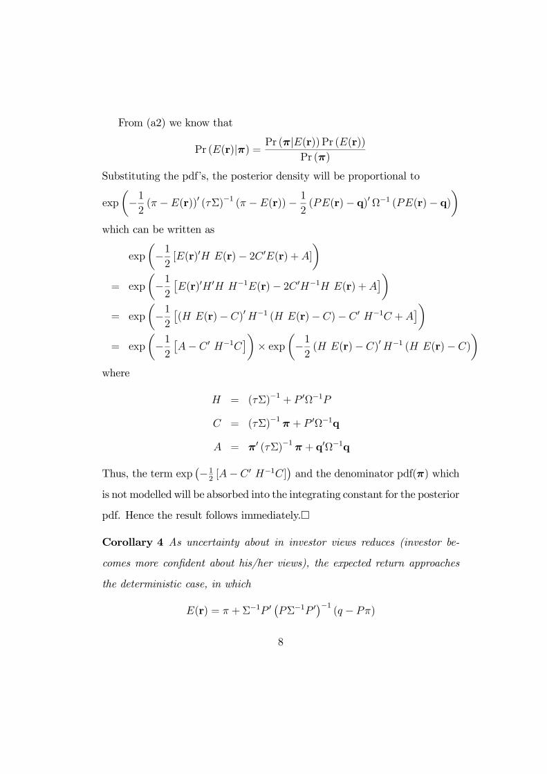
From (a2) we know that

Pr (E(r)|π) = Pr (π|E(r)) Pr (E(r))Pr (π)

Substituting the pdf’s, the posterior density will be proportional to

exp

µ−12(π − E(r))0 (τΣ)−1 (π − E(r))− 1

2(PE(r)− q)0Ω−1 (PE(r)− q)

¶which can be written as

exp

µ−12[E(r)0H E(r)− 2C 0E(r) +A]

¶= exp

µ−12

£E(r)0H 0H H−1E(r)− 2C 0H−1H E(r) +A

¤¶= exp

µ−12

£(H E(r)− C)0H−1 (H E(r)− C)− C 0 H−1C +A

¤¶= exp

µ−12

£A− C 0 H−1C

¤¶× expµ−12(H E(r)− C)0H−1 (H E(r)− C)

¶where

H = (τΣ)−1 + P 0Ω−1P

C = (τΣ)−1π + P 0Ω−1q

A = π0 (τΣ)−1π + q0Ω−1q

Thus, the term exp¡−1

2[A− C 0 H−1C]

¢and the denominator pdf(π) which

is not modelled will be absorbed into the integrating constant for the posterior

pdf. Hence the result follows immediately.¤

Corollary 4 As uncertainty about in investor views reduces (investor be-

comes more confident about his/her views), the expected return approaches

the deterministic case, in which

E(r) = π + Σ−1P 0¡PΣ−1P 0

¢−1(q − Pπ)

8

4 Interpretation of Proposition 3

We have proved that E(r)|π has posterior mean£(τΣ)−1 + P 0Ω−1P

¤−1 £(τΣ)−1π + P 0Ω−1q

¤which can be written as

£(τΣ)−1 + P 0Ω−1P

¤−1 (τΣ)−1π + ¡P 0Ω−1P¢ (P 0P )−1 P 0q| z n×1

Also we know that

P E(r) = q+ v

or that

q = P E(r)−v

which can be seen as a “regression” of q on P , with E(r) being the vector of

unknown (to be estimated) coefficients1. Then

(P 0P )−1 P 0q

can be interpreted as the least squares estimate of expected returns, E(r),

according to investors views

(P 0P )−1 P 0q =[E(r)

Thus, Proposition 3 can be restated in the form

mean of E(r)|π = £(τΣ)−1 + P 0Ω−1P ¤−1 h(τΣ)−1π + ¡P 0Ω−1P¢[E(r)i1of course we need k > n

9

which makes clear how subjective views are combined with data-equilibrium.

The term in the second square brackets is a weighted average of data equilib-

rium π and the least squares estimate of expected returns, [E(r), according

to investors views, the (vector) weights being (τΣ)−1 and (P 0Ω−1P ) respec-

tively.

If the distribution of expected returns around the data equilibrium π is

tight, i.e. τΣ small, then (τΣ)−1 will be large and more weight will be put

to π. If the investor is confident about his/views then Ω is small, resulting

in a large P 0Ω−1P which puts more weight on the least squares views[E(r).

5 Optimal Asset Allocation Recommendations

As we have established in the mean-variance analysis, the vector of weights

of any frontier portfolio can be written as a mixture of any two distinct

frontier portfolios. In fact, these can be the globally-minimum-variance-

portfolio, Σ−1110Σ−11 , and the original portfolio’s zero-covariance portfolio. But

since the latter is a frontier portfolio, it should be a function of the vector

of expected returns. The Black-Litterman model provides a framework to

update subjective views on expected returns with data equilibrium returns

and makes possible to tactically allocate funds according to this process.

References

[1] Black F and R Litterman (1992), Global Portfolio Optimization, Finan-

cial Analysts Journal, September/October, pp 28-43

10

[2] Michaud R (1989), The Markowitz Optimization Enigma: Is Optimized

Optimal?, Financial Analysts Journal, January/February, pp 31-42

[3] Michaud R (1998), Efficient Asset Management, Harvard Business School

Press, Boston, Massachusetts

11