bayesian prediction of deterministic functions, with ... · bayesian prediction of deterministic...

Bayesian Prediction of Deterministic Functions, with Applications to the Design and Analysisof Computer ExperimentsAuthor(s): Carla Currin, Toby Mitchell, Max Morris and Don YlvisakerReviewed work(s):Source: Journal of the American Statistical Association, Vol. 86, No. 416 (Dec., 1991), pp. 953-963Published by: American Statistical AssociationStable URL: http://www.jstor.org/stable/2290511 .

Accessed: 07/12/2012 14:23

Your use of the JSTOR archive indicates your acceptance of the Terms & Conditions of Use, available at .http://www.jstor.org/page/info/about/policies/terms.jsp

.JSTOR is a not-for-profit service that helps scholars, researchers, and students discover, use, and build upon a wide range ofcontent in a trusted digital archive. We use information technology and tools to increase productivity and facilitate new formsof scholarship. For more information about JSTOR, please contact [email protected].

.

American Statistical Association is collaborating with JSTOR to digitize, preserve and extend access to Journalof the American Statistical Association.

http://www.jstor.org

This content downloaded by the authorized user from 192.168.72.223 on Fri, 7 Dec 2012 14:23:18 PMAll use subject to JSTOR Terms and Conditions

http://www.jstor.org/action/showPublisher?publisherCode=astata

http://www.jstor.org/stable/2290511?origin=JSTOR-pdf

http://www.jstor.org/page/info/about/policies/terms.jsp


Bayesian Prediction of Deterministic Functions, With Applications to the Design and Analysis

of Computer Experiments CARLA CURRIN, TOBY MITCHELL, MAX MORRIS, and DON YLVISAKER*

This article is concerned with prediction of a function y(t) over a (multidimensional) domain T, given the function values at a set of "sites" {tm, t 2, ..., tl"} in T, and with the design, that is, with the selection of those sites. The motivating application is the design and analysis of computer experiments, where t determines the input to a computer model of a physical or behavioral system, and y(t) is a response that is part of the output or is calculated from it. Following a Bayesian formulation, prior uncertainty about the function y is expressed by means of a random function Y, which is taken here to be a Gaussian stochastic process. The mean of the posterior process can be used as the prediction function 9(t), and the variance can be used as a measure of uncertainty. This kind of approach has been used previously in Bayesian interpolation and is strongly related to the kriging methods used in geostatistics. Here emphasis is placed on product linear and product cubic correlation functions, which yield prediction functions that are, respectively, linear or cubic splines in every dimension. A posterior entropy criterion is adopted for design; this minimizes the expected uncertainty about the posterior process, as measured by the entropy. A computational algorithm for finding entropy-optimal designs on multidimensional grids is described. Several examples are presented, including a two-dimensional experiment on a computer model of a thermal energy storage device and a six-dimensional experiment on an integrated circuit simulator. Predictions are made using several different families of correlation functions, with parameters chosen to maximize the likelihood. For comparison, predictions are also made via least squares fitting of various polynomial and spline models. The Bayesian design/prediction methods, which do not require any modeling of y, produce comparatively good predictions. For some correlation functions, however, the 95% posterior probability intervals do not give adequate coverage of the true values of y at selected test sites. These methods are fairly simple and offer considerable potential for virtually automatic implementation, although further development is needed before they can be applied routinely in practice.

KEY WORDS: Computer models; Correlation function; Cross-validation; Entropy; Experimental design; Interpolation; Kriging; Optimal design; Spline fitting; Stochastic processes.

1. INTRODUCTION

We are concerned here with the prediction of a function y on a domain T, given the function values at a set of "sites" D = {t0 E T, i = 1, ..., n}, which we are at liberty to select. We shall take T to be in Rk and y(t) to be in R1, although the primary elements of the approach can be described with more general T and y. The motivating application is the design and analysis of computer experiments (Sacks, Welch, Mitchell, and Wynn 1989), where t determines the input to a computer model of a physical or behavioral system and y(t) is a response that is part of the output or is calculated from it. We consider t to be fixed during any given run of the computer model, and we as-

* Carla Currin is a Graduate Student, Department of Psychology, Ohio State University, Columbus, OH 43210. Toby Mitchell and Max Morris are Research Staff Members, Mathematical Sciences Section, Engineer- ing Physics and Mathematics Division, Oak Ridge National Laboratory, Oak Ridge, TN 37831. Don Ylvisaker is Professor, Department of Math- ematics, University of California, Los Angeles, CA 90024. At the time of her contribution to this paper, Carla Currin was a student at Bryn Mawr College visiting Oak Ridge National Laboratory under the Oak Ridge Science and Engineering Research Semester Program, funded by the U.S. Department of Energy through Oak Ridge Associated Universities. Toby Mitchell's and Max Morris's research was supported by the Applied Mathematical Sciences Research Program, Office of Energy Research, U.S. Department of Energy, through Contract DE-AC05-840R21400 with Martin Marietta Energy Systems, Inc. Don Ylvisaker's research was supported by National Science Foundation Grant DMS 86-02018. This work has benefited from the authors' many conversations with Jerry Sacks, William Welch, and Henry Wynn, whose collaboration was started and nurtured by a series of workshops on efficient data collection, funded by National Science Foundation Grant DMS 86-09819. The authors are also grateful to Robert Buck for running the circuit simulator model to provide the data used in the example of Section 4.4.

sume the function y(t) is deterministic: If the program is run twice (on the same computer) with the same value of t, the same value of y will result. In this context, the experiment design consists of the sites in D; the experiment itself consists of running the computer model n times, each time with input determined by a different member of D. Knowledge of the n design sites and the corresponding responses yi, . . *, Yn is then used to predict y(t) at any desired t E T. Interest in prediction derives from the fact that complex computer models often require long running times; the number of runs that can be made is therefore limited. We are concerned here with methods of prediction given D and with the choice of D.

Here we use a Bayesian formulation, under which (un- certain) knowledge about the function y is expressed by means of the random function Y. This usage has previously been applied to surface estimation in several contexts, including interpolation and, more recently, image restoration (Geman and Geman 1984; Ripley 1988, chap. 5). Random functions have been studied for a long time under the head- ing of stochastic processes, and we borrow notation and nomenclature from that source. In particular, we shall refer to the representations of prior and posterior knowledge of y as the prior and posterior processes. The posterior mean of Y given the n-vector of responses YD can be used as the prediction function 9; this is clearly an interpolating function, that is, y(t(')) = y(t(i)), for i = 1, ..., n. Bayesian interpolation has a long history-see Diaconis (1988) for

? 1991 American Statistical Association Journal of the American Statistical Association

December 1991, Vol. 86, No. 416, A Focus on Bayesion Methods

953



954 Journal of the American Statistical Association, December 1991

an interesting account of a method published by Poincare in 1896. More recently, Kimeldorf and Wahba (1970a) es- tablished the connection between Bayesian interpolation and smoothing splines, and Wahba (1978) provided more general results along the same lines. (See, also, Wahba 1990.)

On another front, the use of random functions to represent knowledge about deterministic functions observed with error is central to Bayesian regression methodology. Orig- inally, the prior process was generated simply by assigning a joint prior distribution to the p coefficients in a standard linear regression model (Raiffa and Schlaifer 1961; Tiao and Zeilner 1964; Lindley and Smith 1972). Chaloner (1984) reviewed much of the corresponding work in design of experiments. Because of their finite dimensionality, however, these priors are not well suited to prediction of deterministic functions where there is no observation error. In particular, knowledge of y at p suitably chosen sites is sufficient to predict y at all t with no uncertainty whatever; this seems unrealistic, and leads to obvious difficulties if n > p. We shall not consider finite-dimensional processes further here. Infinite-dimensional processes have been used as Bayesian priors for prediction in regression settings by Blight and Ott (1975) and Wahba (1978); O'Hagen (1978) and Steinberg (1985) used them to develop design criteria as well.

Another large body of work, with a long history and a slightly different philosophy, is based on the view of y as a realization of a stochastic process, that is, Y is taken as a model for y. The prediction of future values of a time series given past values (Parzen 1961) is a particularly well- studied example of the modeling approach. Similar ideas have been widely applied in the analysis of spatial data and support, for example, the kriging methods used in geostatistics. Descriptions of these methods and references to the extensive associated literature are available, for example, in the texts by Journel and Huijbregts (1978), Ripley (1981), and Davis (1986). Sometimes a Bayesian philosophy is mixed in, by assigning subjective priors to the parameters of the model (Kitanidis 1986; Omre 1987). The modeling approach has also been taken for prediction in various settings by Kimeldorf and Wahba (1970b), Sacks and Ylvisaker (1985), Ylvisaker (1987), Sacks, Schiller, and Welch (1989), and Sacks, Welch, Mitchell, and Wynn (1989). The classical best linear unbiased predictor (BLUP) is commonly used to estimate y under this approach.

We interpret Y as a representation of knowledge about y; this is the sense in which we consider our approach to be Bayesian. However, we are deliberately vague about whose knowledge we are representing, and in what situation. We shall favor prior processes that we think could be used by an impartial, if not totally ignorant, Bayesian in a wide range of applications. Such priors will of necessity ignore special information that may be available to the experimenter in a particular case. To relieve some anxiety about the choice of a specific prior, we require only that a class of priors be specified; within that class, the one that performs the best with respect to some cross-validational criterion will be selected. The choice of a class of priors is rather arbitrary, which limits the appeal of the method, although we think

the ones we emphasize here have some attractive features. In any case, once the choice is made, matters proceed fairly smoothly.

An advantage to the use of random functions for prediction is that the variability of Y given YD can be used to provide measures of posterior uncertainty, and designs can be sought to minimize the expected uncertainty in some sense. See Ylvisaker (1987), Sacks, Welch, Mitchell, and Wynn (1989), and Section 3 for references to previous work along these lines. The development of practical design methods has not been extensive, however, particularly for construction of designs for prediction in high-dimensional spaces.

In Section 2, we present the approach we have adopted for prediction. Like many previous authors, we restrict attention to Gaussian prior processes. We are particularly in- terested in the one-dimensional linear and cubic correlation functions (Sections 2.4, 2.5), which, when extended to higher dimensions by the product correlation rule (Section 2.6), yield prediction functions that are, respectively, linear or cubic splines in every dimension. For design, we use a posterior entropy criterion (Section 3.1), which is fundamen- tally similar to the criterion of D-optimality that is used frequently in the design of regression experiments. In Sec- tion 3.2 we describe a computational algorithm for finding entropy-optimal designs on multidimensional grids. We present several examples in Section 4, including one experiment on a computer model of a thermal energy storage device and another on an integrated circuit simulator.

This article is in many respects complementary to that of Sacks, Schiller, and Welch (1989), who first applied spatial stochastic models to the design of computer experiments for prediction, and to that of Sacks, Welch, Mitchell, and Wynn (1989), who discussed this methodology and some of the issues associated with it. Our article, which has different emphases and offers some alternative viewpoints and techniques, is based largely on a technical report (Currin, Mitchell, Morris, and Ylvisaker 1988), which we shall cite for material that is not presented here. The methods described here are still at a relatively early stage of development for general practical use, even though they are based largely on ideas that have been put forward at many different times and places. The hard questions concern the choice of prior process, both for design and for prediction, and the choice of design criteria.

2. PREDICTION

2.1 The Prior and Posterior Processes

We represent prior "knowledge" about the unknown function y(t), t E T, by the Gaussian process Y = {Yt, t E T}, such that, for every finite set of sites S C T, the random vector Ys is multivariate normal with mean vector E[Ys] = ,s and with positive definite covariance matrix cov(Ys, Ys) = ss. Normality is chosen for convenience; the posterior process, given the vector of observed responses YD on the set of design sites D C T, is well known and is also Gaus- sian. Its mean and covariance at any finite set of sites S C T is given by



Currin, Mitchell, Morris, and Ylvisaker: Bayesian Prediction of Deterministic Functions 955

/SID = E[YS I YD] = As + o-SDo-J(YD - AD) (2.1) and

OSSID = COVIYS, YS I YD] = oSS - OSDODDODS, (2.2)

where o0SD = o-'s = cov(Ys, YD). From a Bayesian viewpoint, the posterior process itself is the object of interest; since it is used for prediction, we shall sometimes refer to it as the predictive process. Further reduction to a single prediction function 9 depends on the specification of the loss L(y, 9) incurred when selecting 9. It is well known that if L = (9(t) - y(t))2 at specified t, then the posterior expectation of L is minimized when

Y9(t) = ttID = lt + 0OtDU_DD( YD - AD)* (2.3)

This is by far the most popular choice of prediction function derived from Gaussian prior processes. A notable exception is found in O'Hagan (1978), where 9 is required to be a simple parametric approximating function (e.g., a polynomial of low degree). From an approximation theoretic viewpoint, (2.3) is the unique interpolating function in the span of the n basis functions that appear as elements of o0tD, viewed as functions of t. Here the basis functions follow automatically from the choice of prior process Y and design D and do not need to be chosen explicitly by the user. The function 9 at (2.3) can also be viewed as a minimal norm interpolant; see, for example, Micchelli and Wahba (1981) and Sacks and Ylvisaker (1985).

Since o-DD does not depend on t, predictions can be generated very quickly for a large number of sites once the n- run experiment on the computer model has been completed. The vector o-D(YDD- AD) need be computed only once; it is best obtained as the solution to an n x n system of linear equations.

2.2 Stationarity

Since we are seeking a general method here, we shall not discuss ways of eliciting and implementing problem-specific prior information. Instead, we shall impose some conditions of stationarity, which are intended to produce prior processes that are noninformative, or at least impartial in some respects.

In particular, we shall require that the prior mean and variance be constant for all t in T: A, = ,u, u-t = o-2, and that, at any two sites t and s in T, the prior correlation p,, between Y, and Y, depends only on the difference vector d = t - s through a suitable correlation function R. That is, Pts= R(t - s) = R(d), where R(O) = 1. (The difference vector d is defined, since we assume here that T is in Rk.) Of course, R must be such that for any finite set of sites S, the correlation matrix Pss generated by R is positive definite to satisfy the requirements for Y set out at the begin- ning of Section 2.1.

Under these stationarity restrictions, the prior distribution for Ys at any set of m sites S C T does not change if S is shifted within T. Equations (2.1)-(2.2) become

/LSID = W1r + PSDPDD( YD - ,Jn) (2.4) and

CSSID = C [PSS- PSDP DDPSDS], (2 .5 )

where Jm is an m-vector of l's and Jn is an n-vector of l's. In particular, for prediction at a single site t,

y (t) = Wt|D = / + PtDPDD(YD - pJ) (2.6) and

QJtt|D = (2[ 1 - PtDDPDt]* (2.7)

If desired, a linear model for y could be incorporated by means of a nonstationary prior, either through the mean of Y, or, if the coefficients are assigned prior distributions, through the covariance of Y. The need for this in prediction has not yet become evident to us, however. In the examples we have considered, some of which are presented in Sec- tion 4, predictions based on simple stationary priors are quite good, even when y can be well approximated by a linear model.

A natural way to eliminate ,u and o- from the prior process would be to assign them standard noninformative prior distributions. For fixed R, the posterior distribution for y(t) would be a scaled and shifted Student's t, as one would expect (see, for example, Kitanidis 1986). In this article, however, we shall view ,u and C- as parameters of the prior process and shall handle them as described later.

2.3 The Parameters of the Prior Process

What we have described so far is really a family of Bayesian procedures, indexed by ,u, o-, and whatever parameters 0 may appear in the expression for R. In practice, we choose the member of the family that we think shows the best predictive performance on the function at hand- this suggests cross-validation. Of the various kinds of cross- validation we have tried (Currin et al. 1988), maximum likelihood seems the most reliable. This is an often-used method for estimating the parameters in spatial process models (Wecker and Ansley 1983; Mardia and Marshall 1984; Sacks, Schiller, and Welch 1989; Sacks, Welch, Mitchell, and Wynn 1989). Maximum likelihood estimation is not usually regarded as cross-validation, but consider the following setup. Pick the size ns of a "training sample" S randomly (uniformly) from the integers 0, 1, . . ., n - 1. Then choose S randomly from D and the "test site" s randomly from D - S. Following Geisser and Eddy (1979), define the predictive deficiency to be X = -log p(y3 I ys), where we use p generically to denote a probability density function. Then E(X) = -log p(YD), that is, minimizing the expected predictive deficiency is the same as maximizing the likelihood. [This can be shown through an argument that begins by writing the likelihood in n! ways as P(YD)

= P(Yil)P(yi2 I yil) .. P(Yin Iy, yi 2, .I . ., yinl) and then taking logs on both sides, where il, i2, ..., in is a permu- tation of 1, 2, ..., n.]

The log likelihood is

L = --{n log(2i,) + n log 2 + logjpDD(0)j

1 + 27 (YD - JJfl)T[PDD(O9)F1(YD - ,Jn)

where dependence on 0 is now explicitly indicated in the




notation. Maximization over ,u and o- yields the well-known formulas

JT[PDD(O)1JYD

and 1

2()= -(YD - (O)Jn )T[PDD(O)F1(YD - (0y)J n

Determination of 0 is usually done by constrained iterative search. This can require a considerable amount of computation, depending on the dimension of 0. We have not yet encountered a situation where different starting values led to appreciably different final values, but some authors have reported the existence of local optima (Warnes and Ripley 1987; Ripley 1988, chap. 2). Unfortunately, there is sometimes not enough information in the data to distin- guish well among competing values of (0, o-). This would not matter if the posterior process were insensitive to joint changes in 0 and o- in the region of high likelihood, but one cannot expect such behavior.

2.4 Linear Correlation Functions in One Dimension

In the simple one-dimensional case with T = [0, 1], consider the well known correlation functions

1 1 R(d) = I1-- Jd|, 2< 0< o? (2.8)

0 2 and

R(d)= 1-IdI, l di<0; 0

= 0, dl 0. (2.9)

We shall refer to (2.8) as the linear correlation function, and to (2.9) as the nonnegative linear correlation function. In the absence of much prior information about y, the latter is more appealing, since it has the property that, for any 0, uncertainty about y(s) given a single observation at t is non- decreasing as the distance of s from t increases. For both of these correlation functions, the ith element of PtD is a linear spline, so 9(t) is a linear spline interpolating function. [See Equation (2.6).]

2.5 Cubic Correlation Functions in One Dimension

It is well known that the result of integrating a stochastic process is to produce a process that is "smoother" in various senses. This technique can be used to derive useful candidates for prior processes in the present setting. Sup- pose, for example, that there is a stationary Gaussian process Y on T = [0, 1] whose first derivative Y is a stationary Gaussian process having the linear correlation function given by (2.8). Mitchell, Morris, and Ylvisaker (1990) found necessary and sufficient conditions for the existence of such a process. Its correlation function has the form

R(d) = 1 - -l d2 + 2 Id13, (2.10)

where 01 and 02 are positive parameters that satisfy 02 C 2O1 and 02- 60102 + 12O12 ' 2402.

Since 9(t) is a linear combination of n functions of the form R(t - t(i)), the interpolating function that follows from the choice of cubic R at (2.10) is seen to be a cubic spline. Another correlation function that produces cubic splines is the nonnegative cubic correlation

R(d) = 1- 6(-) + 6(! !) ' d| < 2

= 2(1 _ Idl I cdl < 0,

= 0, IdI 2 0, (2.11)

where 0 > 0. This correlation function can be obtained by letting Y, be the integral from t to t + 0/2 of a process with nonnegative linear correlation R(d) = 1 - 21dj/0, for |dl < 0/2, and R(d) = 0, for |dl 2 0/2. An advantage of the nonnegative cubic correlation is that 0 can be made as small as desired, thus permitting very local prediction. It also re- quires only one parameter rather than two, which makes the task of maximizing the likelihood easier.

There are, of course, numerous other candidates for correlation functions. See, for example, Journel and Hu- ijbregts (1978), Mitchell et al. (1990), Young (1977), and Steinberg (1985). One guiding principle is simplicity since, asymptotically at least, it does not matter which member of an equivalence class of correlation functions is selected (Stein 1987). Not much else, however, is known about the relationship between the prior process and predictive performance on particular classes of true response functions.

2.6 Extension to More Dimensions

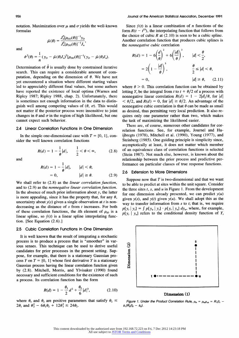
Suppose now that T is two-dimensional and that we want to be able to predict at sites within the unit square. Consider the three sites t, s, and u in Figure 1. From the development for one dimension already presented, we can predict y(u) given y(s), and y(t) given y(u). We shall adopt this as the way to transfer information from s to t; that is, we require P[Yt I Ys] = f p[yu I Y] P[Yt I yU] dyu, where, for example, P[Yt YU] refers to the conditional density function of Yt

0~~~~~~~~~~~~ N

.o I

t *---- _ lu{

Dimension (1)

Figure 1. Under the Product Correlation Rule, Pts = PtuPus = R1('t1 -

s1)R2(t2 - 82).




given Yu = y,. Since Yt, Y, and Y, are jointly Gaussian, it can be shown that this holds if and only if Pts = ptupus Under our assumptions of stationarity, this becomes Pts = R1(t- u)R2(u2 - s2) = RI(t - s)R2(t2 - s2), where R1 and R2 are correlation functions for one-dimensional processes. The same reasoning leads us in k dimensions to the product correlation rule, by which we define

k k

Pts= H Rj(tj - s) = H Rj(dJ), (2.12) j=1 j=l

where t and s are in Rk and Rj (j = 1, 2, ...,k), are correlation functions for one-dimensional processes. This rule has been used previously for prediction in spatial settings, for example, Ylvisaker (1975). [Connections with splines are noted by Chen, Gu, and Wahba (1989)].

In situations where a single predictor variable is represented by a point in more than one dimension (like "lo- cation" on a two-dimensional surface), the selection of the coordinate axes for representing that point may be arbitrary. Then one might modify (2.12) by requiring the correlation between the responses at two locations (with the other variables fixed) to depend, for example, on the Eu- clidean distance between them. There are examples of such correlation functions in the literature on kriging and on thin plate splines. When each variable has a distinct physical meaning, however, the use of an isotropic distance between two sites as a basis for choosing the form of the correlation function loses its intuitive appeal.

In this article, we adopt the product correlation rule as given in (2.12). For example, in k dimensions, the linear correlation (2.8) becomes

R(d) = H (1 |dj. (2.13)

We generally allow each dimension to have its own correlation parameter(s), although this complicates the problem of maximizing the likelihood.

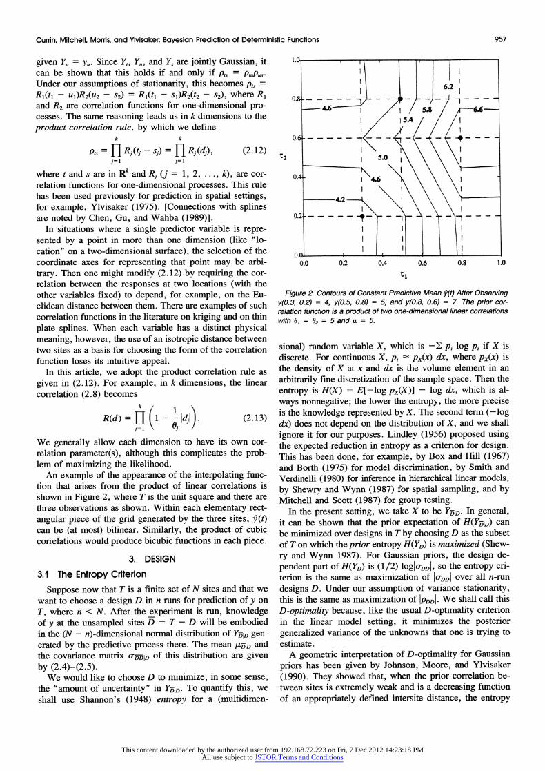
An example of the appearance of the interpolating function that arises from the product of linear correlations is shown in Figure 2, where T is the unit square and there are three observations as shown. Within each elementary rectangular piece of the grid generated by the three sites, 9(t) can be (at most) bilinear. Similarly, the product of cubic correlations would produce bicubic functions in each piece.

3. DESIGN

3.1 The Entropy Criterion

Suppose now that T is a finite set of N sites and that we want to choose a design D in n runs for prediction of y on T, where n < N. After the experiment is run, knowledge of y at the unsampled sites D = T - D will be embodied in the (N - n)-dimensional normal distribution of Y-JD generated by the predictive process there. The mean gID and the covariance matrix 0-DTID of this distribution are given by (2.4)-(2.5).

We would like to choose D to minimize, in some sense, the "amount of uncertainty" in YD-ID. To quantify this, we shall use Shannon's (1948) entropy for a (multidimen-

1.0 l ' _ l

6.2

0 .-- - --

4.6 5.8 6.6- I / 5.4// 1

0.6 -

t2 I'--n-WNX_ t2 ~~~~~~5.0

0.4- 4.6 1 \ 1\\ \ \

4.2

0.2. _ _ 4 _ _ _ _ _ _

0.0 0.0 0.2 0A 0.6 0.8 1.0

tl

Figure 2. Contours of Constant Predictive Mean 9(t) After Observing y(0.3, 0.2) = 4, y(0.5, 0.8) = 5, and y(0.8, 0.6) = 7. The prior correlation function is a product of two one-dimensional linear correlations with 01 = 02 = 5 and A = 5.

sional) random variable X, which is -E pi log pi if X is discrete. For continuous X, pi px(x) dx, where px(x) is the density of X at x and dx is the volume element in an arbitrarily fine discretization of the sample space. Then the entropy is H(X) = E[-log px(X)] - log dx, which is al- ways nonnegative; the lower the entropy, the more precise is the knowledge represented by X. The second term (-log dx) does not depend on the distribution of X, and we shall ignore it for our purposes. Lindley (1956) proposed using the expected reduction in entropy as a criterion for design. This has been done, for example, by Box and Hill (1967) and Borth (1975) for model discrimination, by Smith and Verdinelli (1980) for inference in hierarchical linear models, by Shewry and Wynn (1987) for spatial sampling, and by Mitchell and Scott (1987) for group testing.

In the present setting, we take X to be YID-I In general, it can be shown that the prior expectation of H(YTID) can be minimized over designs in T by choosing D as the subset of T on which the prior entropy H(YD) is maximized (Shew- ry and Wynn 1987). For Gaussian priors, the design dependent part of H(YD) is (1/2) log1o-DD1, so the entropy criterion is the same as maximization of IoDDI over all n-run designs D. Under our assumption of variance stationarity, this is the same as maximization of IPDDI. We shall call this D-optimality because, like the usual D-optimality criterion in the linear model setting, it minimizes the posterior generalized variance of the unknowns that one is trying to estimate.

A geometric interpretation of D-optimality for Gaussian priors has been given by Johnson, Moore, and Ylvisaker (1990). They showed that, when the prior correlation between sites is extremely weak and is a decreasing function of an appropriately defined intersite distance, the entropy




criterion maximizes the minimum distance among design points and favors those designs with the fewest pairs whose intersite distance matches this minimum.

The tendency of D-optimality to maximize intersite distances is also evident in augmenting existing designs. Shew- ry and Wynn's (1987) result, applied to the one-point aug- mentation of an n-run design, implies that the optimal site for the new observation is one at which the predictive variance (after the first n runs) is maximum. This usually oc- curs at sites that are remote from the existing ones.

The question of which design criterion to use is still quite open, in spite of the considerable attention given elsewhere to the minimization of the average posterior variance on T (or, under the modeling approach, average mean squared error). See, for example, O'Hagan (1978), Micchelli and Wahba (1981), Sacks and Ylvisaker (1985), Steinberg (1985), Sacks, Schiller, and Welch (1989), and Sacks, Welch, Mitchell, and Wynn (1989). Another intuitively appealing criterion, which involves some computational difficulty in practice, is the minimization of the maximum posterior variance. See Johnson et al. (1990) for an interesting geometric interpretation of this criterion.

A practical weakness of design optimality for fixed R is that one seldom knows, at design time, what correlation function will be selected for the analysis. This difficulty has a parallel in optimal design for regression experiments, where the optimal design is highly dependent on the choice of regression model, which is not usually made until the data are analyzed. A pragmatic approach there is to base the design on weaker prior information than one expects to in- voke in the analysis (e.g., use a cubic rather than a linear or quadratic polynomial model for design). We adopt a similar approach in the examples of Section 4, choosing R(d) to decay rapidly as |dl increases for the purpose of design construction.

If the experiment is done in several stages, one can design each stage using a correlation function chosen on the basis of data from the preceding stages. The sequential modification of the prior is an attempt to approximate what would be accomplished by a full Bayesian approach, in which R is itself assigned a vague prior, but which is much more intractable. There are some examples of two-stage designs in Currin et al. (1988), but we found the second-stage design to be generally less effective than we had expected. For the present article, we shall consider only one-stage designs.

3.2 Design Algorithm

The computation of optimal designs in this setting is dif- ficult, especially in several dimensions, and there have been few attempts at algorithms other than the one we describe below. Sacks and Schiller (1988), in trying to minimize the maximum posterior variance, used various exchange algorithms as well as simulated annealing, with mixed results. Sacks, Schiller, and Welch (1989) and Sacks, Welch, Mitchell and Wynn (1989) used a standard quasi-Newton optimization routine for minimization of the average posterior variance.

The designs constructed for this article are all based on the entropy criterion (D-optimality). They were obtained from a computer algorithm adapted from DETMAX (Mitchell 1974), which was first developed for the purpose of con- structing D-optimal designs for linear regression. The optimization method is based on a series of "excursions," which are sequences of designs in which each design differs from its predecessor by the presence or absence of a single site. All additions and deletions are made with the goal of maximizing the determinant of the correlation matrix for the resulting design. As noted above, the best site t to add to an existing design D is the one at which the variance function ,2tD is greatest. The search for this site is conducted over a grid in T. Except when T has few dimensions or the grid is very coarse, it is not practical to make the search exhaustive. Instead we have incorporated a multiple search procedure that can best be envisioned by thinking of a set of n hikers trying to climb a hill. Each hiker starts at one of the n current design sites; at each of these the variance function is zero. The search for the maximum variance proceeds by stages, where, in each stage, each hiker takes one step in the direction that maximizes that hiker's altitude. We restrict each hiker to consider only the neighboring grid points associated with a change in exactly one of the k design variables, so at most 2k possibilities exist-fewer if - the hiker is at a boundary of T. Under this procedure, the variance function (2.7) is evaluated at (at most) 2nk sites in each stage. Sometimes two hikers will merge, in which case they continue as one. The search ends when all hikers have stopped at (local) maxima; the site that corresponds to the largest of these is taken to be the best site to bring into the design at the current point in the excursion.

When required to delete a site, the algorithm makes use of the fact that the largest determinant after deletion of a site in D can be achieved by choosing that site to be the one associated with the greatest element of the diagonal of PDD Straightforward methods are used for updating pDD

1 and loglpDDj as each excursion proceeds.

Except in very simple cases, the algorithm is unlikely to produce a globally optimal design, although the use of excursions does give it some capability for escaping local optima. We usually make several tries, and choose the best result. When the number of candidates is large, as will usually be required for experiments in many dimensions, this can take a nontrivial amount of computing time. (See Sec- tion 4.4 for a specific example.) It is the nature of the algorithm, however, to make most of its progress during the first few iterations, so reasonably good designs can be achieved without waiting for the algorithm to run to its natural stopping point.

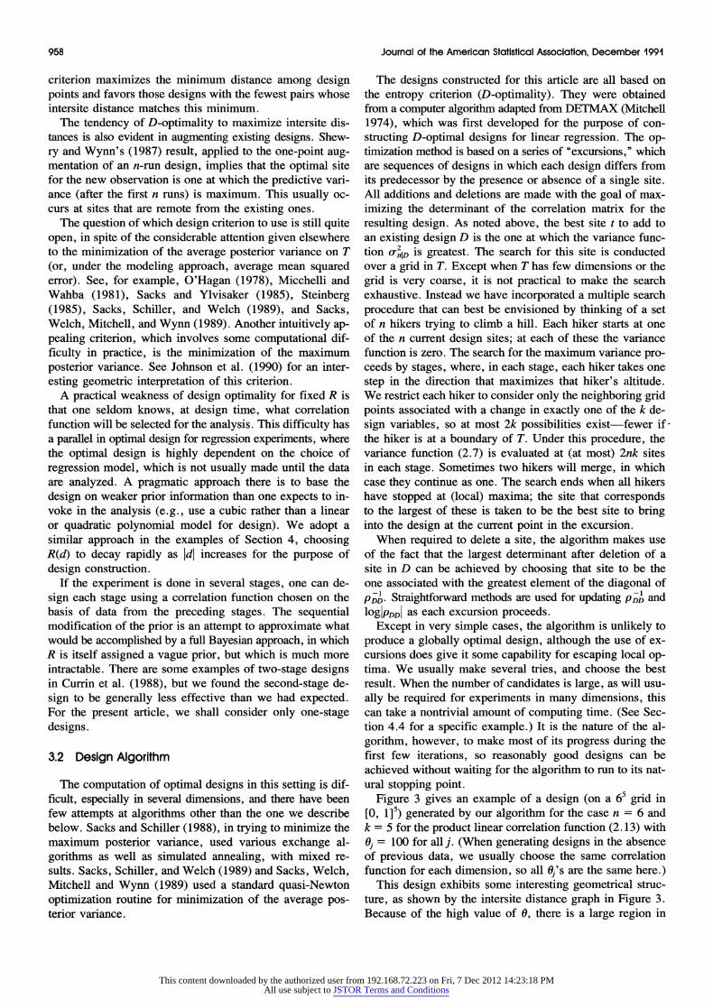
Figure 3 gives an example of a design (on a 65 grid in [0, 1]5) generated by our algorithm for the case n = 6 and k = 5 for the product linear correlation function (2.13) with Oj= 100 for all j. (When generating designs in the absence of previous data, we usually choose the same correlation function for each dimension, so all 61's are the same here.)

This design exhibits some interesting geometrical structure, as shown by the intersite distance graph in Figure 3. Because of the high value of 0, there is a large region in




SITE t1 t2 t3 t4 t5

1 0 0 0 0 0 2 0.6 0 1 1 0 3 0 0.6 1 0 1 4 1 1 0.6 0 0 5 1 0 0 0.6 1 6 0 1 0 1 0.6

6

' r _5~~~@

Figure 3. The Design Generated by our D-Optimality Algorithm for Five Design Variables and Six Runs, on a 65 Grid in [0, 1]5, Based on the Product Linear Correlation Function (Eq. 2.13) With Common 0 = 100. The graph below the design depicts the intersite distances, where the distances are defined by d(t, s) = lj5-j I tj - sj I, and the distances are 2.6 (----- ), 2.8 (- - -), and 3.2 ()

the middle of T in which there are no design sites; predictions here rely heavily on information from the suffounding design sites.-

At the other extreme, designs that infiltrate T to a greater extent can be constructed by using correlation functions R(d) that decrease rapidly with |d|. An example is the product exponential coffelation

R(d ) = tI exp(- oIdjj) = (xp- E )dl

0>0 31

with large values of 0. As 0 increases, these designs approach the "maximin distance" designs of Johnson et al. (1990), where intersite distance is defined as lldjl. Exam- ples of designs based on (3. 1) are given in the next section.

4. EXAMPLES

4.1 Introduction

In this section we discuss the application of the methods of this article to three examples. In the first, the data are generated by a known test function, although we shall treat it as an unknown function evaluated by a computer model. In the last two examples, real computer models are used. In all three examples, the likelihood criterion was used to determine the parameters of the prior process.

4.2 Test Function in Two Dimensions

The data were generated by the function

y(tl, t2) =[ 1 - exp( 1 /(2t2)/

230t3 l90t2+ 292t+ 6 . ^+3 snv21 + /

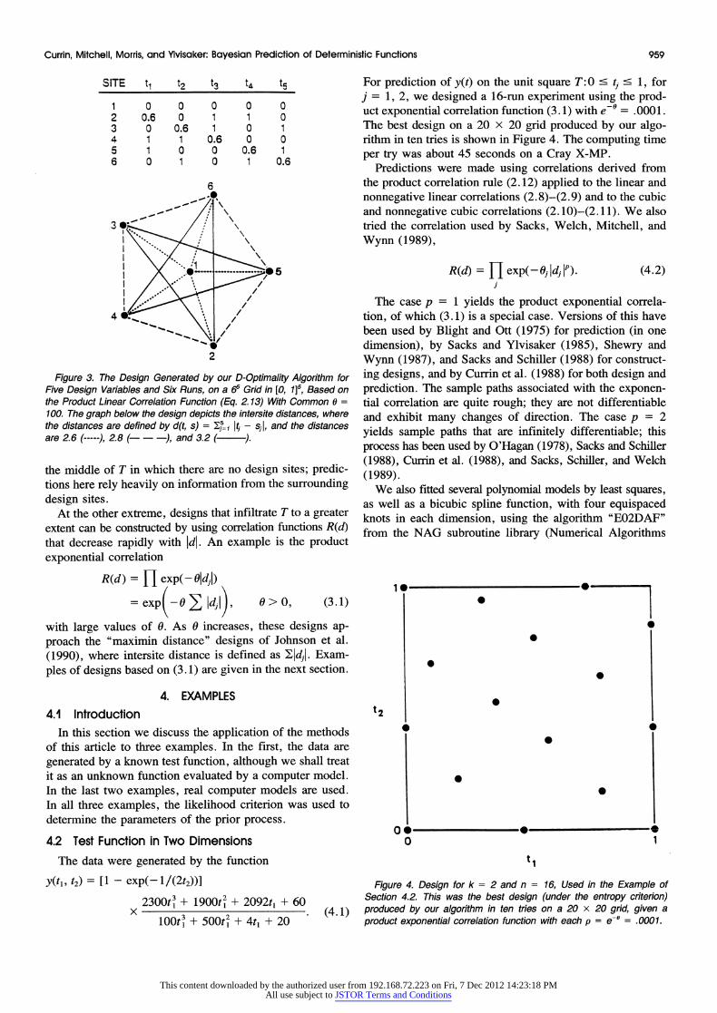
For prediction of y(t) on the unit square T:0 ' tj ' 1, for j = 1, 2, we designed a 16-run experiment using the product exponential correlation function (3.1) with e-0 = .0001. The best design on a 20 x 20 grid produced by our algorithm in ten tries is shown in Figure 4. The computing time per try was about 45 seconds on a Cray X-MP.

Predictions were made using correlations derived from the product correlation rule (2.12) applied to the linear and nonnegative linear correlations (2.8)-(2.9) and to the cubic and nonnegative cubic correlations (2.10)-(2. 11). We also tried the correlation used by Sacks, Welch, Mitchell, and Wynn (1989),

R(d) = f1 exp(-O OIdj IP) (4.2) i

The case p = 1 yields the product exponential correlation, of which (3.1) is a special case. Versions of this have been used by Blight and Ott (1975) for prediction (in one dimension), by Sacks and Ylvisaker (1985), Shewry and Wynn (1987), and Sacks and Schiller (1988) for construct- ing designs, and by Currin et al. (1988) for both design and prediction. The sample paths associated with the exponential correlation are quite rough; they are not differentiable and exhibit many changes of direction. The case p = 2 yields sample paths that are infinitely differentiable; this process has been used by O'Hagan (1978), Sacks and Schiller (1988), Cunin et al. (1988), and Sacks, Schiller, and Welch (1989).

We also fitted several polynomial models by least squares, as well as a bicubic spline function, with four equispaced knots in each dimension, using the algorithm "EO2DAF" from the NAG subroutine library (Numerical Algorithms

iS0

0

*

t2

* f

O 1 tt

Figure 4. Design for k = 2 and n = 16, Used in the Example of Section 4.2. This was the best design (under the entropy criterion) produced by our algorithm in ten tries on a 20 x 20 grid, given a product exponential correlation function with each p = e0@ = .0001.




Table 1. Summary of Prediction Errors for the Two-Dimensional Test Function (4.1), for Several Prediction Methods

Error Max. RMS Int. Int. Design Predictor D.F R2 error error width covg.

r Bayes (SWMW) - - 2.17 .55 .79 .45 | Bayes (C) - 2.45 .60 1.42 .79 | Bayes (C+) - 2.61 .70 1.81 .83

Figure 4 ) Bayes (L, L+) - 3.10 .70 5.18 .99 Cubic Poly. 6 93.8 3.70 .91 7.83 1.00 4 x 4 Bicubic Spline 0 100.0 5.73 .98 Quadratic Poly. 10 76.5 5.72 1.64 9.99 .98 Bicubic Poly. 0 100.0 22.28 4.07 - Bicubic Poly. 0 100.0 3.53 1.04 - Cubic Poly. 6 98.9 4.19 1.11 3.58 .91 Bayes (C) - 4.89 1.41 2.20 .71 Bayes (C+) - 5.27 1.59 2.45 .69

4 x 4 Bayes (L, L+) - 5.92 1.62 6.43 .94 |Bayes (SWMW) -5.44 1.63 2.02 .59 Quadratic Poly. 10 86.3 6.05 1.90 8.05 .94

V 4 x 4 Bicubic Spline 0 100.0 7.60 2.72

NOTE: Correlation functions used for Bayesian prediction are: linear (L), nonnegative linear (L+), cubic (C), nonnegative cubic (C+), and Equation (4.2) (SWMW). Quadratic, cubic, and bicubic polynomials were also fit by the method of least squares, as was a bicubic spline with knots on a regular 4 x 4 grid. The maximum absolute error and the root mean squared (RMS) error are evaluated on a set of 400 random test sites. Int. width refers to the average width of the 95% posterior probability intervals; nt. covg. is the proportion of the test sites at which the interval covered the true value of y. For the least squares fits, the regression R2 and the degrees of freedom for error are also given. Results are given for two 16-run designs: the one shown in Figure 4 and a 4 x 4 factorial design.

Group, Inc. 1987). The fitting equation supplied by this algorithm has 36 coefficients. Since there were only 16 runs, the algorithm automatically chose the interpolating solution that minimizes the sum of squares of the coefficients. We repeated the whole exercise using a 4 x 4 factorial design (with levels 0, .33333, .66667, 1) instead of the design in Figure 4.

The errors in y(t) at 400 test sites (the same for all methods) chosen randomly from a uniform distribution on T, are summarized in Table 1. Also shown, for each method, is the average width of the 95% posterior probability intervals

at the 400 test sites and the proportion of test sites at which the true y(t) is covered by the interval.

The poor performance of the bicubic polynomial approximation for our design can be attributed to the near sin- gularity of the least squares equations for fitting that model to data from that design. The least squares prediction equation in this case is a wildly fluctuating interpolator.

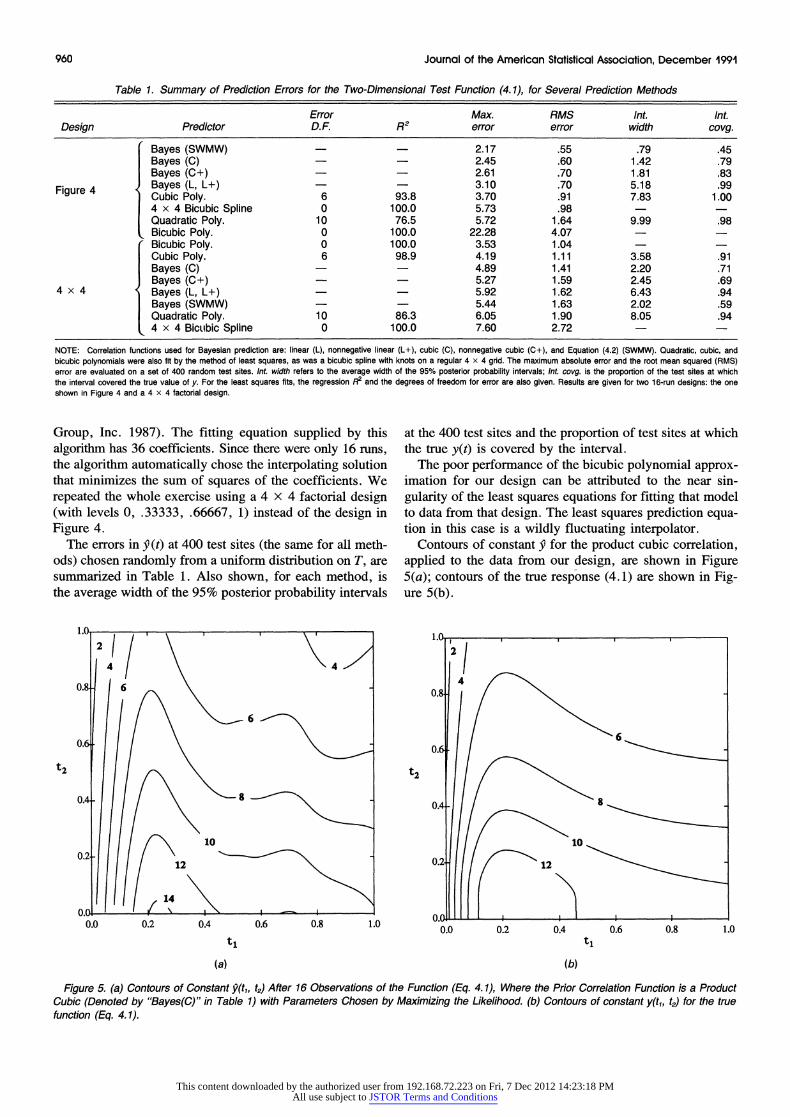
Contours of constant 9 for the product cubic correlation, applied to the data from our design, are shown in Figure 5(a); contours of the true response (4.1) are shown in Fig- ure 5(b).

1. I I1.c I

02/// 2/l 1?/ 11

0.8 6 0.8

6

0. ~~~~~~~~~~~~~~~~~~~~~~~~~~6 0. ~~~~~~~~~~~~~~~~~~~~~~~~~0. t2 t2

0A.4 8 0.- 8

10 10 0.2 0.2 12

121

14 0.0 II 0.0 0.2 0.4 0.6 0.8 1.0 0*C 0.0 0.2 0.4 0.6 0.8 1.0

ti ti

(a) (b)

Figure 5. (a) Contours of Constant k'tl, t2) After 16 Observations of the Function (Eq. 4. 1), Where the Prior Correlation Function is a Product Cubic (Denoted by "Bayes(C)" in Table 1) with Parameters Chosen by Maximizing the Likelihood. (b) Contours of constant y(tl, t2) for the true function (Eq. 4. 1).




Table 2. Design and Responses for Our Nine-run Experiment on the TWOLAYER Model

t, t2 y

.0000 .3333 .5056

.0000 1.0000 .4290

.2500 .0000 .5288

.2500 .6667 .2383

.5000 .9167 .0354

.5833 .2500 .0000

.8333 .5833 .0000 1.0000 .0000 .0000 1.0000 1.0000 .0000

NOTE: Variables t1 (melting temperature of one layer) and t2 (thickness of that layer) are each scaled to the interval [0, 1]. The response y is the utility index.

4.3 Thermal Energy Storage System Example (Two Dimensions)

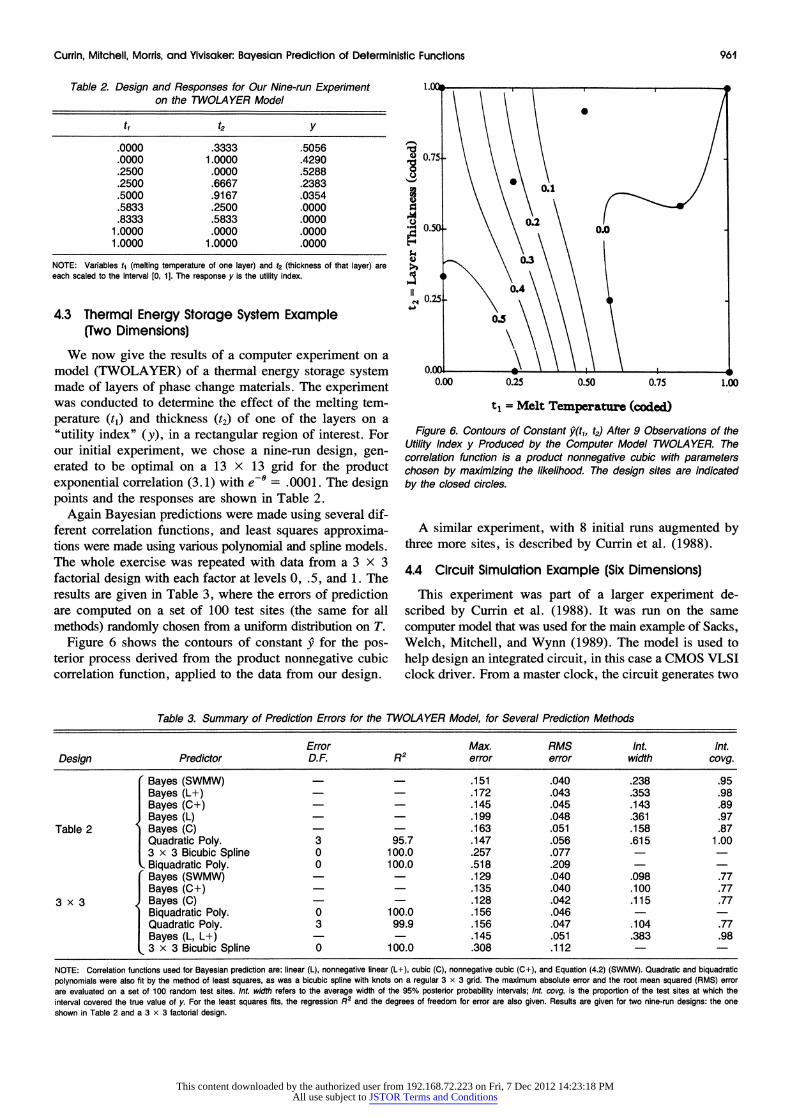
We now give the results of a computer experiment on a model (TWOLAYER) of a thermal energy storage system made of layers of phase change materials. The experiment was conducted to determine the effect of the melting temperature (tl) and thickness (t2) of one of the layers on a "utility index" (y), in a rectangular region of interest. For our initial experiment, we chose a nine-run design, generated to be optimal on a 13 x 13 grid for the product exponential correlation (3.1) with e-0 = .0001. The design points and the responses are shown in Table 2.

Again Bayesian predictions were made using several different correlation functions, and least squares approxima- tions were made using various polynomial and spline models. The whole exercise was repeated with data from a 3 x 3 factorial design with each factor at levels 0, .5, and 1. The results are given in Table 3, where the errors of prediction are computed on a set of 100 test sites (the same for all methods) randomly chosen from a uniform distribution on T.

Figure 6 shows the contours of constant 9 for the posterior process derived from the product nonnegative cubic correlation function, applied to the data from our design.

1.0 .

0 75.

0.1

o.oo 0.2s o.so 0.7s .200

4) ~~~03

ii ~~~~0.4 el0.25.

0.5

0.1 0.00 0.25 0.50 0.75 1.00

tj = Melt Temperature (coded)

Figure 6. Contours of Constant 9(t1, t2j After 9 Observations of the Utility Index y Produced by the Computer Model TWOLAYER. The correlation function is a product nonnegative cubic with parameters chosen by maximizing the likelihood. The design sites are indicated by the closed circles.

A similar experiment, with 8 initial runs augmented by three more sites, is described by Currin et al. (1988).

4.4 Circuit Simulation Example (Six Dimensions)

This experiment was part of a larger experiment described by Currin et al. (1988). It was run on the same computer model that was used for the main example of Sacks, Welch, Mitchell, and Wynn (1989). The model is used to help design an integrated circuit, in this case a CMOS VLSI clock driver. From a master clock, the circuit generates two

Table 3. Summary of Prediction Errors for the TWOLAYER Model, for Several Prediction Methods

Error Max. RMS Int. Int. Design Predictor D.F. R2 error error width covg.

(Bayes (SWMW) .151 .040 .238 .95 Bayes (L+) .172 .043 .353 .98 Bayes (C +) .145 .045 .143 .89

J Bayes (L) .199 .048 .361 .97 Table 2 Bayes (C) - .163 .051 .158 .87

Quadratic Poly. 3 95.7 .147 .056 .615 1.00 3 x 3 Bicubic Spline 0 100.0 .257 .077 Biquadratic Poly. 0 100.0 .518 .209

(Bayes (SWMW) - .129 .040 .098 .77 | Bayes (C+) .135 .040 .100 .77

3 x 3 ) Bayes (C) - .128 .042 .115 .77 Biquadratic Poly. 0 100.0 .156 .046

| Quadratic Poly. 3 99.9 .156 .047 .104 .77 Bayes (L, L+) .145 .051 .383 .98

_ 3 x 3 Bicubic Spline 0 100.0 .308 .112

NOTE: Correlation functions used for Bayesian prediction are: linear (L), nonnegative linear (L+), cubic (C), nonnegative cubic (C+), and Equation (4.2) (SWMW). Quadratic and biquadratic polynomials were also fit by the method of least squares, as was a bicubic spline with knots on a regular 3 x 3 grid. The maximum absolute error and the root mean squared (RMS) error are evaluated on a set of 100 random test sites. Int. width refers to the average width of the 95% posterior probability intervals; Int. covg. is the proportion of the test sites at which the interval covered the true value of y. For the least squares fits, the regression R2 and the degrees of freedom for error are also given. Results are given for two nine-run designs: the one shown in Table 2 and a 3 x 3 factorial design.




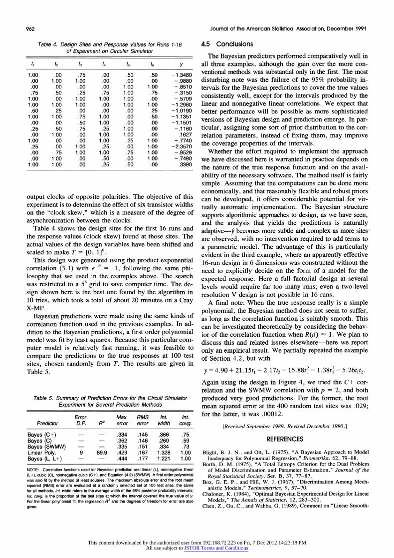
Table 4. Design Sites and Response Values for Runs 1-16 of Experiment on Circular Simulator

tt t2 t3 t4 t5 t6 Y

1.00 .00 .75 .00 .50 .50 -1.3480 .00 1.00 1.00 .00 .00 .00 -.9880 .00 .00 .00 .00 1.00 1.00 -.8510 .75 .50 .25 .75 1.00 .75 -.3150

1.00 .00 1.00 1.00 1.00 .00 -.5709 1.00 1.00 1.00 .00 1.00 1.00 -1.2960 .50 .25 .00 .00 .00 .25 -1.0190

1.00 1.00 .75 1.00 .00 .50 -1.1351 .00 .00 .50 1.00 .00 .00 -1.1501 .25 .50 .75 .25 1.00 .00 -.1160 .00 1.00 .00 1.00 1.00 .00 .1627

1.00 .00 .00 1.00 .25 1.00 -.7740 .25 .00 1.00 .25 .00 1.00 -2.3570 .00 .75 1.00 1.00 .75 1.00 -.9529 .00 1.00 .00 .50 .00 1.00 -.7490

1.00 1.00 .00 .25 .50 .00 .3390

output clocks of opposite polarities. The objective of this experiment is to determine the effect of six transistor widths on the "clock skew," which is a measure of the degree of asynchronization between the clocks.

Table 4 shows the design sites for the first 16 runs and the response values (clock skew) found at those sites. The actual values of the design variables have been shifted and scaled to make T = [0, 1]6.

This design was generated using the product exponential correlation (3.1) with e-@ = .1, following the same philosophy that we used in the examples above. The search was restricted to a 56 grid to save computer time. The design shown here is the best one found by the algorithm in 10 tries, which took a total of about 20 minutes on a Cray X-MP.

Bayesian predictions were made using the same kinds of correlation function used in the previous examples. In ad- dition to the Bayesian predictions, a first order polynomial model was fit by least squares. Because this particular computer model is relatively fast running, it was feasible to compare the predictions to the true responses at 100 test sites, chosen randomly from T. The results are given in Table 5.

Table 5. Summary of Prediction Errors for the Circuit Simulator Experiment for Several Prediction Methods

Error Max. RMS Int. Int. Predictor D.F. R2 error error width covg.

Bayes (C+) - .334 .145 .366 .75 Bayes (C) .362 .146 .260 .59 Bayes (SWMW) .335 .151 .334 .73 Linear Poly. 9 89.9 .429 .167 1.328 1.00 Bayes (L, L+) .444 .177 1.221 1.00

NOTE: Correlation functions used for Bayesian prediction are: linear (L), nonnegative linear (L+), cubic (C), nonnegative cubic (C+), and Equation (4.2) (SWMW). A first order polynomial was also fit by the method of least squares. The maximum absolute error and the root mean squared (RMS) error are evaluated at a randomly selected set of 100 test sites, the same for all methods. Int. width refers to the average width of the 95% posterior probability intervals; Int. covg. is the proportion of the test sites at which the interval covered the true value of y. For the linear polynomial fit, the regression R2 and the degrees of freedom for error sre also given.

4.5 Conclusions

The Bayesian predictors performed comparatively well in all three examples, although the gain over the more con- ventional methods was substantial only in the first. The most disturbing note was the failure of the 95% probability intervals for the Bayesian predictions to cover the true values consistently well, except for the intervals produced by the linear and nonnegative linear correlations. We expect that better performance will be possible as more sophisticated versions of Bayesian design and prediction emerge. In particular, assigning some sort of prior distribution to the correlation parameters, instead of fixing them, may improve the coverage properties of the intervals.

Whether the effort required to implement the approach we have discussed here is warranted in practice depends on the nature of the true response function and on the avail- ability of the necessary software. The method itself is fairly simple. Assuming that the computations can be done more economically, and that reasonably flexible and robust priors can be developed, it offers considerable potential for virtually automatic implementation. The Bayesian structure supports algorithmic approaches to design, as we have seen, and the analysis that yields the predictions is naturally adaptive-y becomes more subtle and complex as more sites- are observed, with no intervention required to add terms to a parametric model. The advantage of this is particularly evident in the third example, where an apparently effective 16-run design in 6 dimensions was constructed without the need to explicitly decide on the form of a model for the expected response. Here a full factorial design at several levels would require far too many runs; even a two-level resolution V design is not possible in 16 runs.

A final note: When the true response really is a simple polynomial, the Bayesian method does not seem to suffer, as long as the correlation function is suitably smooth. This can be investigated theoretically by considering the behavior of the correlation function when R(d) 1. We plan to discuss this and related issues elsewhere-here we report only an empirical result. We partially repeated the example of Section 4.2, but with

y = 4.90 + 21.15t, - 2.17t2 - 15.88t 2 - 1.38t2 - 5.26tlt2.

Again using the design in Figure 4, we tried the C+ correlation and the SWMW correlation with p = 2, and both produced very good predictions. For the former, the root mean squared error at the 400 random test sites was .029; for the latter, it was .00012.

[Received September 1989. Revised December 1990.]

REFERENCES

Blight, B. J. N., and Ott, L. (1975), "A Bayesian Approach to Model Inadequacy for Polynomial Regression," Biometrika, 62, 79-88.

Borth, D. M. (1975), "A Total Entropy Criterion for the Dual Problem of Model Discrimination and Parameter Estimation," Journal of the Royal Statistical Society, Ser. B, 37, 77-87.

Box, G. E. P., and Hill, W. J. (1967), "Discrimination Among Mech- anistic Models," Technometrics, 9, 57-70.

Chaloner, K. (1984), "Optimal Bayesian Experimental Design for Linear Models," The Annals of Statistics, 12, 283-300.

Chen, Z., Gu, C., and Wahba, G. (1989), Comment on "Linear Smooth-




ers and Additive Models," by A. Buja, T. Hastie, and R. Tibshirani, The Annals of Statistics, 17, 515-521.

Currin, C., Mitchell, T., Morris, M., and Ylvisaker, D. (1988), "A Bayesian Approach to the Design and Analysis of Computer Experi- ments," ORNL-6498, available from National Technical Information Service, 5285 Port Royal Road, Springfield, VA 22161.

Davis, J. C. (1986), Statistics and Data Analysis in Geology (2nd ed.), New York: John Wiley.

Diaconis, P. (1988), "Bayesian Numerical Analysis," in Statistical De- cision Theory and Related Topics IV (vol. 1), eds. S. S. Gupta and J. 0. Berger, New York: Springer-Verlag, 163-175.

Geisser, S., and Eddy, W. F. (1979), "A Predictive Approach to Model Selection," Journal of the American Statistical Association, 74, 153- 160; correction, 75, 765.

Geman, S., and Geman, D. (1984), "Stochastic Relaxation, Gibbs Dis- tributions, and the Bayesian Restoration of Images," IEEE Transac- tions on Pattern Analysis and Machine Intelligence, 6, 721-741.

Johnson, M., Moore, L., and Ylvisaker, D. (1990), "Minimax and Max- imin Distance Designs," Journal of Statistical Planning and Inference, 26, 131-148.

Journel, A. G., and Huijbregts, C. J. (1978), Mining Geostatistics, New York: Academic Press.

Kimeldorf, G. S., and Wahba, G. (1970a), "A Correspondence Between Bayesian Estimation on Stochastic Processes and Smoothing by Splines," The Annals of Mathematical Statistics, 41, 495-502.

(1970b), "Spline Functions and Stochastic Processes," Sankhya, Ser. A, 32, 173-180.

Kitanidis, P. K. (1986), "Parameter Uncertainty in Estimation of Spatial Functions: Bayesian Analysis," Water Resources Research, 22, 499- 507.

Lindley, D. V. (1956), "On a Measure of the Information Provided by an Experiment, " The Annals of Mathematical Statistics, 27, 986-1005.

Lindley, D. V., and Smith, A. F. M. (1972), "Bayes' Estimates for the Linear Model," Journal of the Royal Statistical Society, Ser. B, 34, 1-18.

Mardia, K. V., and Marshall, R. J. (1984), "Maximum Likelihood Es- timation of Models for Residual Covariance in Spatial Regression," Biometrika, 71, 135-146.

Micchelli, C. A., and Wahba, G. (1981), "Design Problems for Optimal Surface Interpolation," Approximation Theory and Applications, ed. Z. Ziegler, New York: Academic Press.

Mitchell, T. J. (1974), "An Algorithm for the Construction of 'D-Opti- mal' Experimental Designs," Technometrics, 16, 203-210.

Mitchell, T., Morris, M., and Ylvisaker, D. (1990), "Existence of Smoothed Stationary Processes on an Interval," Stochastic Processes and Their Applications, 35, 109-119.

Mitchell, T. J., and Scott, D. S. (1987), "A Computer Program for the Design of Group Testing Experiments," Communications in Statis- tics-Theory and Methods, 16, 2943-2955.

Numerical Algorithms Group, Inc. (1987), The NAG Fortran Library Manual (Mark 12), Downers Grove, IL: Author.

O'Hagan, A. (1978), "Curve Fitting and Optimal Design for Prediction" (with discussion), Journal of the Royal Statistical Society, Ser. B, 40, 1-42.

Omre, H. (1987), "Bayesian Kriging-Merging Observations with Qual- ified Guesses in Kriging," Mathematical Geology, 19, 25-39.

Parzen, E. (1961), "An Approach to Time Series Analysis," The Annals of Mathematical Statistics, 32, 951-989.

Raiffa, H., and Schlaifer, R. (1961), Applied Statistical Decision Theory, Cambridge, MA: Harvard University Press.

Ripley, B. D. (1981), Spatial Statistics, New York: John Wiley. (1988), Statistical Inference for Spatial Processes, New York:

Cambridge University Press. Sacks, J., and Schiller, S. (1988), "Spatial Designs," Fourth Purdue

Symposium on Statistical Decision Theory and Related Topics, ed. S. S. Gupta, New York: Academic Press.

Sacks, J., Schiller, S. B., and Welch, W. J. (1989), "Designs for Com- puter Experiments," Technometrics, 31, 41-47.

Sacks, J., Welch, W. J., Mitchell, T. J., and Wynn, H. P. (1989), "De- sign and Analysis of Computer Experiments," (with comments) Sta- tistical Science, 4, 409-435.

Sacks, J., and Ylvisaker, D. (1985), "Model Robust Design in Regres- sion: Bayes Theory," Proceedings of the Berkeley Conference in Honor of Jerzy Neyman and Jack Kiefer, (vol. II), eds. L. M. Le Cam and R. A. Olshen, Monterey, CA: Wadsworth, pp. 667-679.

Shannon, C. E. (1948), "A Mathematical Theory of Communication," The Bell System Technical Journal, 27, 379-423, 623-656.

Shewry, M. C., and Wynn, H. P. (1987), "Maximum Entropy Sam- pling," Journal of Applied Statistics, 14, 165-170.

Smith, A. F. M., and Verdinelli, I. (1980), "A Note on Bayes Designs for Inference Using a Hierarchial Linear Model," Biometrika, 67, 613- 619.

Stein, M. L. (1987), "Uniform Asymptotic Optimality of Linear Predic- tions of a Random Field Using an Incorrect Second-Order Structure," Technical Report 214, University of Chicago, Dept. of Statistics.

Steinberg, D. M. (1985), "Model Robust Response Surface Designs: Scaling Two-Level Factorials," Biometrika, 72, 513-526.

Tiao, G. C., and Zellner, A. (1964), "Bayes' Theorem and the Use of Prior Knowledge in Regression Analysis," Biometrika, 51, 219-230.

Wahba, G. (1978), "Improper Priors, Spline Smoothing and the Problem of Guarding Against Model Errors in Regression," Journal of the Royal Statistical Society, Ser. B, 40, 364-372.

(1990), Spline Models for Observational Data, (CBMS-NSF Re- gional Conference Series in Applied Mathmatics, Vol. 59), Philadel- phia: Society for Industrial and Applied Mathematics.

Warnes, J. J., and Ripley, B. D. (1987), "Problems with Likelihood Estimation of Covariance Functions of Spatial Gaussian Processes," Biometrika, 74, 640-642.

Wecker, W. E., and Ansley, C. F. (1983), "The Signal Extraction Ap- proach to Nonlinear Regression and Spline Smoothing," Journal of the Amerian Statistical Association, 78, 81-89.

Ylvisaker, D. (1975), "Designs on Random Fields," A Survey of Statis- tical Design and Linear Models, ed. J. N. Srivastava, Amsterdam: North- Holland.

(1987), "Prediction and Design," The Annals of Statistics, 15, 1-19.

Young, A. S. (1977), "A Bayesian Approach to Prediction Using Poly- nomials," Biometrika, 64, 309-317.



bayesian prediction of deterministic functions, with ... · bayesian prediction of deterministic...

Documents