bayesian speaker verification with heavy-tailed priors · f known as an i-vector (e.g. f = 400)....

Gaussian PLDAHeavy-tailed PLDA

Directional scattering

Bayesian Speaker Verification withHeavy-Tailed Priors

Patrick Kenny

Odyssey Speaker and Language Recognition Workshop

June 29, 2010

1 / 41 Patrick Kenny Bayesian Speaker Verification



Introduction

The low dimensional i-vector representation of speechsegments opens up new possibilities for using Bayesianmethods in speaker recognition.You can go a long way with Bayesian methods under theassumptions that speaker and channel effects areGaussian and statistically independent.You can do better by relaxing the Gaussian assumption. Inparticular, it seems to be possible to do away with scorenormalization in speaker verification.The directional scattering behavior which appears toexplain the success of cosine distance scoring in speakerrecognition can be modeled by relaxing the statisticalindependence assumption. (This part of the talk isspeculative.)




Joint Factor Analysis with i-vectors

Each recording is represented by a single vector of dimensionF known as an i-vector (e.g. F = 400).

Given a speaker and i-vectors D1, . . . , DR we assume

Dr = S + Cr

whereR is the number of recordings of the speaker, indexed by rS depends on the speaker, Cr depends on the channelS and Cr are statistically independent (?)S and Cr are multivariate Gaussian (?)

To begin with, we assume both statistical independence andGaussianity.




Probabilistic Linear Discriminant Analysis

PLDAUnder Gaussian assumptions, this model is known in facerecognition as PLDA [Prince and Elder].

The between-speaker covariance matrix is Cov(S, S).

The within-speaker covariance matrix is Cov(Cr , Cr ) (assumedto be independent of r ).

If the feature dimension F is high, these matrices cannot betreated as full rank.




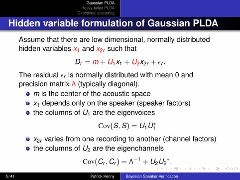
Hidden variable formulation of Gaussian PLDA

Assume that there are low dimensional, normally distributedhidden variables x1 and x2r such that

Dr = m + U1x1 + U2x2r + εr .

The residual εr is normally distributed with mean 0 andprecision matrix Λ (typically diagonal).

m is the center of the acoustic spacex1 depends only on the speaker (speaker factors)the columns of U1 are the eigenvoices

Cov(S, S) = U1U∗1

x2r varies from one recording to another (channel factors)the columns of U2 are the eigenchannels

Cov(Cr , Cr ) = Λ−1 + U2U2∗.




Graphical model for Gaussian PLDA

Including x2r enables the decomposition

Cov(Cr , Cr ) = Λ−1 + U2U2∗.

This is not needed in all cases and, under Gaussianassumptions, x2r can always be eliminated at recognition time(later).




Working assumptions

Assume for the time being thatwe have succeeded in estimating the model parameters(m, U1, U2,Λ)

given a collection D = (D1, . . . , DR) of i-vectors associatedwith a speaker, we have figured out how to evaluate themarginal likelihood (“the evidence”)

P(D) =

∫P(D, h)dh

where h represents the entire collection of hidden variablesassociated with the speaker.

We will show how to do speaker recognition in this situation andhow both of these problems can be tackled by using variationalBayes to approximate the posterior distribution P(h|D).




PLDA speaker recognition

Given two i-vectors D1 and D2 suppose we wish to perform thehypothesis test

H1 : The speakers are the sameH0 : The speakers are the different.

The likelihood ratio is

P(D1, D2|H1)

P(D1|H0)P(D2|H0).

Every term here is an evidence integral of the form∫P(D, h)dh.

The likelihood ratio for any type of speaker recognition orspeaker clustering problem can be written down just as easily.




Approximating the evidence

The evidence P(D) can be evaluated exactly in the Gaussiancase but this involves inverting large (sparse) block matrices[Prince and Elder].

Even in the Gaussian case, it is more efficient to use avariational approximation: if Q(h) is any distribution on h and

L = E[ln

P(D, h)

Q(h)

]then

L ≤ ln P(D)

with equality iff Q(h) = P(h|D) [Bishop].

Variational Bayes provides a principled way of finding a goodapproximation Q(h) to P(h|D).




Why are posteriors generally intractable?

There is nothing mysterious about the posterior P(h|D). ByBayes rule,

P(h|D) =P(D|h)P(h)

P(D).

The problem in practice is that the normalizing constant 1/P(D)— the evidence — cannot be evaluated:

P(D) =

∫P(D|h)P(h)dh.

Another way of stating the difficulty is that whateverfactorizations (i.e. statistical independence assumptions) existin the prior P(h) are destroyed in the posterior by taking theproduct P(D|h)P(h).




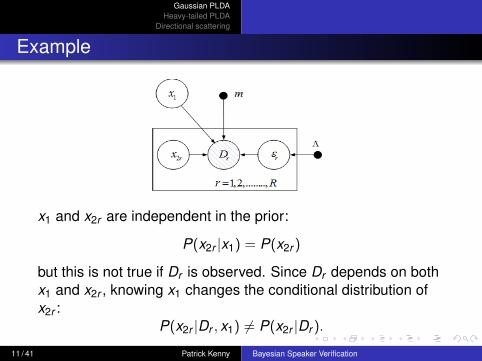
Example

x1 and x2r are independent in the prior:

P(x2r |x1) = P(x2r )

but this is not true if Dr is observed. Since Dr depends on bothx1 and x2r , knowing x1 changes the conditional distribution ofx2r :

P(x2r |Dr , x1) 6= P(x2r |Dr ).




Variational Bayes

Set x2 = (x21, . . . , x2R). x1 and x2 are independent in the priorbut they are correlated in the posterior.

The idea in variational Bayes is to force independence in theposterior so that we seek an approximation to P(x1, x2|D) of theform

Q(x1, x2) = Q(x1)Q(x2).

Q(x1) and Q(x2) are estimated by the standard update formulas

ln Q(x1) = Ex2 [ln P(D, x1, x2)] + constln Q(x2) = Ex1 [ln P(D, x1, x2)] + const

which do not involve inverting large block matrices and areguaranteed to increase the value of L on each iteration[Bishop].




The variational posterior is also the key to estimatingthe model parameters

The model parameters (m, U1, U2,Λ) are estimated bymaximizing the evidence criterion∑

s

L(s)

where s ranges over all of the speakers in a training set.

We defined

L = E[ln

P(D, h)

Q(h)

].

It is convenient to decompose this as

L = E [ln P(D|h)]− KL (Q(h)||P(h)) .

Note that the second term does not involve the modelparameters at all.




Maximum likelihood estimation

As a first step towards maximizing the evidence, we sum thecontributions from the first term over all training speakers∑

s

E [ln P(D(s)|h(s)]

and maximize this with respect to the model parameters. Werefer to this as maximum likelihood estimation.

This expression is formally the same as the EM auxiliaryfunction in probabilistic principal components analysis [Bishop].

The only difference is that the expectations are evaluated withthe variational posteriors rather than the true posteriors.




Minimum divergence estimation

Another way to increase the value of the objective function is tofind affine transformations of the model parameters and hiddenvariables

(m, U1, U2,Λ) → (m′, U ′1, U ′

2,Λ′)

h(s) → h′(s)

which preserve the value of the EM auxiliary function butminimize the sum of divergences∑

s

KL(Q′(h′(s)||P(h(s)

).

We refer to this as minimum divergence estimation.




Example

Applying this to the speaker factors x1(s) amounts to finding anaffine transformation such that the posterior moments of x ′

1(s)agree with those of the prior on average:

1S

∑s

Cov(x ′1(s), x ′

1(s)) = I

1S

∑s

E[x ′

1(s)]

= 0

where S is the number of speakers in the training set. Themodel parameters are then updated by applying the inversetransformation to m and U1 so as to preserve the value of theEM auxiliary function.

Interleaving maximum likelihood and minimum divergenceestimation helps to accelerate convergence.




Variational Bayes allows other possibilities to beexplored . . .

These estimation procedures are adequate for speakerrecognition but hard-core Bayesians would avoid pointestimates of the model parameters altogether.

For example, it is possible to put a prior on U1 and calculate aposterior with variational Bayes.

In theory, even the number of speaker factors could be treatedas a hidden variable, rather than a parameter that has to bemanually tuned. (Analogous to the the treatment of the numberof mixture components in Bayesian estimation of Gaussianmixture models [Bishop].)

There is an extensive literature on Bayesian principalcomponents analysis.




Replacing the Gaussian distribution by Student’s t

The Student’s t distribution is a heavy tailed distribution in thesense that the density P(x) has the property that there is apositive exponent k such that

P(x) = O(||x ||−k )

as ||x || → ∞. Compare this with the Gaussian distribution:

P(x) = O(e−||x ||2/2).

Like the Gaussian distribution, the Student’s t distribution isunimodal but it is less susceptible to some well known problemsof Gaussian modeling:

The Gaussian assumption effectively prohibits largedeviations from the mean (“Black Swans”)Maximum likelihood estimation of a Gaussian (i.e. leastsquares) can be thrown off by outliers.




Definition of Student’s t suitable for variational Bayes

The Student’s t distribution can be represented as a continuousmixture of Gaussians, using a construction based on theGamma distribution.

The Gamma distribution G(a, b) is a unimodal distribution onthe positive reals whose density is given by

P(u) ∝ ua−1e−bu (u > 0).

The parameters a and b enable the mean and the variance tobe adjusted independently:

E [u] = a/bVar(u) = a/b2.




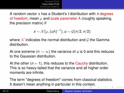
A random vector x has a Student’s t distribution with n degreesof freedom, mean µ and scale parameter Λ (roughly speaking,the precision matrix) if

x ∼ N (µ, (uΛ)−1), u ∼ G(n/2, n/2)

where N indicates the normal distribution and G the Gammadistribution.

At one extreme (n →∞) the variance of u is 0 and this reducesto the Gaussian distribution.

At the other (n = 1), this reduces to the Cauchy distribution.This is so heavy-tailed that the variance and all higher ordermoments are infinite.

The term "degrees of freedom" comes from classical statistics.It doesn’t mean anything in particular in this context.




Example

To make the distribution of the channel factors x2r heavy-tailed,introduce a scalar hidden variable u2r :

x2r ∼ N (0, u−12r I) where u2r ∼ G(n2/2, n2/2)




Graphical model for heavy-tailed PLDA

In heavy-tailed PLDA all of the hidden variables x1, x2r and εrhave Student’s t distributions:

Extra hidden variables: u1, u2r and υr .

Extra parameters: the numbers of degrees of freedom n1, n2and ν.




Variational Bayes carries over straightforwardly

Heavy-tailed PLDA is fully diagonalizable — only diagonalmatrices need to be inverted for variational Bayes (see thepaper).

If n2 = ν, the channel factors x2r can be eliminated atrecognition time and variational Bayes converges very quickly.

Idea: Let P be the orthogonal matrix whose columns are theeigenvectors of the effective covariance matrix Λ−1 + U2U2

∗.Rotate both the model and the data by P to obtain anequivalent model with a diagonal residual precision matrix andno channel factors.

The numbers of degrees of freedom n1, n2 and ν can beestimated (by divergence minimization) using the evidencecriterion.




Gaussian vs. Student’s t on telephone data

Gaussian Student’s tEER/DCF EER/DCF

short2-short3 3.6% / 0.014 2.2% / 0.0108conv-short3 3.7% / 0.009 1.3% / 0.00510sec-10sec 16.4% / 0.070 10.9% / 0.053

NIST 2008 SRE English language female dataEER = equal error rate, DCF = 2008 detection cost functionunnormalized likelihood ratios




The effect of score normalization

Gaussian Student’s tEER/DCF EER/DCF

short2-short3 2.7% / 0.013 2.4% / 0.0128conv-short3 1.5% / 0.009 0.8% / 0.00710sec-10sec 13.3% / 0.063 12.8% / 0.066

likelihood ratios normalized with s-norm (see the paper)helpful in the Gaussian case, harmful for Student’s tone exception (EER 0.8% for 8conv-short3), notstatistically significanteven with normalization, Student’s t is better than Gaussian




Score normalization is usually needed in order to set atrial-independent decision threshold for speaker verification. Itis typically fragile and computationally expensive.

A good generative model for speech should produce likelihoodratios which do not need to be normalized (or even calibrated).

Score normalization is needed in practice because outlyingrecordings tend to produce exceptionally low scores for all ofthe trials in which they are involved.

In the Student’s t case, the hidden variables u1, u2r and υrseem to model these outliers adequately.




The curious case of microphone speech

For telephone speechGaussian PLDA with score normalization gives resultswhich are comparable to cosine distance scoringHeavy-tailed PLDA without score normalization givesbetter results. The error rates are about 25% lower than fortraditional Joint Factor Analysis.

For microphone speech heavy-tailed PLDA breaks down in aninteresting way.




In a companion paper, we describe an i-vector extractorsuitable for speaker recognition with both microphone andtelephone speech (F = 600).

Using only telephone speech, we first trained a model withoutchannel factors

Dr = m + U1x1 + εr

with a full precision matrix for the residual εr .

We augmented this with channel factors trained only onmicrophone speech:

Dr = m + U1x1 + U2r x2r + εr .




It turns out that the microphone channel factors are Cauchydistributed (n2 < 1).

Speaker recognition breaks down unless the model isconstrained (by flooring the number of degrees of freedom) sothat microphone transducer effects have finite variance.

In this case, Student’s t modeling is no better than Gaussian.

Perhaps the best course would be to project away thetroublesome dimensions using linear discriminant analysis(classical LDA or PLDA).




How can this behavior be modeled probabilistically?

Plots of GMM supervectors for different speakers (Tang, Chuand Huang, ICASSP 2009) illustrating directional scattering.The x and y axes are essentially the first two i-vectorcomponents.




Caution: The directional scattering effect in these plots isprobably exaggerated. The utterances are conversation turns(which may be very short), not conversation sides, and theauthors use relevance MAP, not eigenvoice MAP, to estimatesupervectors. An artifact of relevance MAP is that the longer anutterance, the further the supervector from the origin.

Still, directional scattering seems to be the only possibleexplanation for the success of cosine distance scoring inspeaker recognition. (But does anybody know how to accountfor it?)

There appears to be a principal axis of session variability whichvaries from one speaker to another. This is inconsistent withthe assumption that speaker and session effects are additiveand statistically independent.




A proposal for modeling directional scattering

Instead of representing a speaker by a single point x1 in thespeaker factor space, we could represent the speaker by adistribution specified by a mean vector µ and a precisionmatrix Λ. (This is different from the F × F residual precisionmatrix previously denoted by Λ.)

i-vectors are generated by sampling “speaker factors” from thisdistribution:

Dr = m + U1x1r + U2x2r + εr .

The trick is to choose a prior P(µ,Λ) in which µ and Λ are notstatistically independent. Since point estimation of µ and Λ ishopeless, it is necessary to integrate over µ and Λ with respectto the prior P(µ,Λ). Do this with variational Bayes.




The Normal-Wishart prior

To generate observations for a speaker: First, generate anN × N precision matrix Λ (where N is the dimension of thespeaker factors) by sampling from a standard Wishart prior

Λ ∼ W(I, τ).

The Wishart distribution with parameters W and τ , W(W , τ), isa generalization of the Gamma distribution. It is concentratedon positive definite N ×N matrices Λ and its density is given by:

P(Λ) ∝ |Λ|(τ−N−1)/2 exp(−1

2Tr

(W−1Λ)

)).

τ is the number of degrees of freedom: the larger τ , the morepeaked the distribution. There is no loss in generality assuminga standard Wishart prior, W = I (other possibilities could beaccommodated by modifying U1).




Next, generate the mean vector µ for the speaker by samplingfrom a Student’s t distribution with scale parameter Λ andhidden variable w :

µ ∼ N (0, (wΛ)−1), w ∼ G(α/2, β/2).

where, like τ , α and β are parameters to be estimated. We willget to the question of why a Student’s t distribution is neededhere in a moment. (Again, there is no loss of generality intaking the mean of this Student’s t distribution to be 0.)

Since the distribution of µ depends on Λ and w , Λ and µ are notstatistically independent in the prior:

P(Λ|µ) 6= P(Λ)

so there is some hope of modeling speaker-dependentdirectional scattering.




Finally, generate “speaker factors” x1r for each the speaker’srecordings by sampling from a Student’s t distribution withmean µ and scale parameter Λ:

x1r ∼ N (µ, (u1rΛ)−1), u1r ∼ G(n1/2, n1/2).

The difference between the “speaker factors” x1r and thechannel factors x2r is that the distribution of x2r is assumed tobe speaker-independent whereas the model for x1r includesspeaker-dependent hidden variables Λ, µ and w .

Thus x1r models both speaker variability and a particular typeof session variability.




Graphical model for x1r

The values of the parameters α, β and τ determine whether thismodel exhibits speaker-dependent directional scattering or not.




How can this capture directional scattering?

Compare the speaker-dependent distribution of the covariancematrix Λ−1 with the speaker-independent distribution:

E[Λ−1|w , µ

]=

τ − N − 1τ − N

E[Λ−1

]+

1τ − N

wµµ∗.

The effect of the second term (a rank 1 covariance matrix) is toaugment the variance in direction of the speaker’s mean vectorµ:




Because µµ∗ is weighted by 1τ−N w , the strength of this effect

depends on τ and the parameters α and β which govern thedistribution of w :

E [w ] = α/β

Var(w) = 2α/β2.

If α and β are such that the mean of w is large and the varianceis small, there is marked directional scattering for mostspeakers. (This flexibility is achieved by taking P(µ|Λ) to beStudents t rather than Gaussian.)

On the other hand if β = τ−1 and τ →∞, this model can beshown to reduce to heavy-tailed PLDA and there is nospeaker-dependent directional scattering.

How well this works remains to be seen . . .




Conclusion

Gaussian PLDA is an effective model for speaker recognition,even though it is based on questionable assumptions, namelythat speaker and channel effects are additive, statisticallyindependent and normally distributed.

These assumptions can be relaxed by adding hidden variablesu1, u2r , υr to model outliers and µ,Λ, w to model directionalscattering.

The derivation of the variational Bayes update formulas ismechanical and, because variational Bayes comes with EM-likeconvergence guarantees, implementations can be debugged.




Caveat: In practice, to do the variational Bayes derivations, theprior distributions of the hidden variables need to be in theexponential family. For example, if you try to do heavy-tailedPLDA with the text book definition of Student’s t, you will getnowhere.

I believe that in order to get the full benefit of Bayesianmethods, you need informative priors whose parameters canbe elicited from training data. (This view is sometimes referredto as “empirical Bayes”.)

For example, the priors on the additional hidden variablesu1, u2r , υr and µ,Λ, w — namely the degrees of freedomn1, n2, ν and τ, α, β — can be estimated from training datausing the evidence criterion.




References for Bayesian Methods

S. J. D. Prince and J. H. Elder, “Probabilistic lineardiscriminant analysis for inferences about identity,” in Proc.11th International Conference on Computer Vision, Rio deJaneiro, Brazil, Oct. 2007, pp. 1–8.

C. Bishop, Pattern Recognition and Machine Learning.New York, NY: Springer Science+Business Media, LLC,2006.

P. Kenny, “Bayesian Speaker Verification with Heavy-TailedPriors” in Proc. Odyssey Speaker and LanguageRecognition Workshop, Brno, Czech Republic, June 2010.http://www.crim.ca/perso/patrick.kenny


http://www.crim.ca/perso/patrick.kenny

bayesian speaker verification with heavy-tailed priors · f known as an i-vector (e.g. f = 400)....

Documents