bayesian statistics for small area estimation - bias project · bayesian statistics for small area...

Bayesian Statistics for Small Area Estimation

V. Gomez-Rubio, N. Best, S. Richardson, G. LiDepartment of Epidemiology and Public HealthImperial College LondonSt. Mary’s Campus, Norfolk PlaceW2 1PG London - United KingdomTel: +44 (0) 20 759 43302 - Fax: +44 (0) 20 740 22150

and Philip ClarkeOffice for National Statistics, United Kingdom

Abstract. National statistical offices are often required to provide statistical infor-mation about characteristics of the population, such as mean income or unem-ployment rate, at several administrative or small area levels. Having good arealevel estimates is important because policies will often be based on this type ofinformation.

In this paper we describe how Bayesian hierarchical models can help in the task ofproviding good quality small area estimates. Starting from direct estimates ob-tained from survey data, we describe a range of Bayesian hierarchical modelsthat incorporate different types of random effects and show that these give im-proved estimates. Models that synthesise individual and aggregated informationare considered as well. Finally, we highlight some additional applications thatfurther exploit the estimates produced, such as the classification and ranking ofareas and how to approach the problem of having no direct information in severalareas.

Keywords: Bayesian Hierarchical Models; Missing Data; Policy Making; SmallArea Estimation; Spatial Models

1. Introduction

Small Area Estimation (Rao, 2003) tackles the important statistical problem ofproviding reliable estimates of a target variable in a set of small geographicalareas. The main difficulty is that it is nearly always impossible to measurethe value of the target variable for all the individuals in the areas of interestand, hence, a survey is conducted to obtain a representative sample (Cochran,1977). Surveys are often designed to include different sorts of data in order to

E-mail: [email protected]

2 V. Gomez-Rubio et al.

make the best use of them. The information collected is used to produce somedirect estimate of the target variable that relies only on the survey design andthe sampled data. Unfortunately, sampling from all areas can be expensive inresources and time. A more practical approach is to select a subset of areaswhere the survey is conducted; estimates for all areas are then produced usingthe sample and some additional auxiliary information which must be availablefor all small areas (Sarndal et al., 1992).

Regression models are often used in this context to provide estimates forthe non-sampled areas. The model is fitted on data from the sample and usedtogether with additional information from auxiliary data to compute estimatesfor non-sampled areas. This method is often known as synthetic estimation(Gonzalez, 1973).

Regression estimators can be extended to include random effects, which canbe estimated by Empirical Best Linear Unbiased Predictors (usually known asEBLUP estimators, see Robinson, 1991). Jiang and Lahiri (2006) provide a re-view on this topic for small area estimation. In addition to the usual covariates,mixed-effect models include random effects to model different types of individ-ual variation and space and time interactions (Singh et al., 2005; Petrucci andSalvati, 2005). Different types of responses can be modelled with this frame-work, but the computations for non-Normal responses can be quite involvedand techniques such as Penalised Quasi-Likelihood are required (Breslow andClayton, 1993). EURAREA Consortium (2004) make a summary of direct andmodel-based likelihood-based small area estimators for several target variablesfor different national datasets from different countries.

The potential of spatial and spatio-temporal modelling in Small Area Es-timation has been addressed by Jiang and Lahiri (2006) and the discussiontherein. The two main benefits that they point out are the possibility of borrow-ing information from neighbouring areas when estimating spatially-correlatedrandom effects and improving estimation in non-sampled areas. Petrucci andSalvati (2005) have also addressed the use of spatial random effects to produceimproved Small Area estimates.

Bayesian alternatives of both the non-spatial and spatial mixed effects mod-els for Small Area Estimation have been proposed (see, for example, Datta andGhosh (1991), Ghosh et al. (1998), and Rao (2003) for a recent review). Inparticular, Bayesian small area spatial modelling has already been successful inother similar contexts, such as the estimation of the rate of disease in differentgeographic regions (Best et al., 2005). Complex mixed-effects and correlationbetween areas can be easily handled and modelled hierarchically in differentlayers of the model. For example, Besag et al. (1991) propose a spatial modelin which the area variation not explained by the available covariates is splitinto two components: one which is unstructured (and independent) for each

Bayesian Statistics for Small Area Estimation 3

area and another one which reflects likely correlation between neighbouring re-gions. Note that disease mapping applications are based on data available ondisease status for all individuals in every area, whilst Small Area Estimationis usually based on a survey which provides access to a limited sample of thepopulation under study and does not cover all areas, hence creating its own setof methodological issues.

Although implementation of complex Bayesian models requires computa-tionally intensive Markov Chain Monte Carlo simulation algorithms (Gilks et al.,1995), there are a number of potential benefits of the Bayesian approach forsmall area estimation. It offers a coherent framework that can handle differenttypes of target variable (e.g. continuous, dichotomous, categorical), differentrandom effects structures (e.g. independent, spatially correlated), areas with nodirect survey information, models to smooth the survey sample variance esti-mates, and so on, in a consistent way using the same computational methodsand software whatever the model. Uncertainty about all model parameters isautomatically captured by the posterior distribution of the small area estimatesand any functions of these (such as their rank), and by the predictive distribu-tion of estimates for small areas not included in the survey sample. Bayesianmethods are particularly well suited to sparse data problems (for example, whenthe survey sample size per area is small) since Bayesian posterior inference isexact (modulo Monte Carlo simulation error associated with the estimation algo-rithms) and does not rely on asymptotic arguments. The posterior distributionobtained from a Bayesian model also provides a much richer output than thetraditional point and interval estimates from a corresponding likelihood-basedmodel. In particular, the ability to make direct probability statements aboutunknown quantities — for example, the probability that the target variable ex-ceeds some specified threshold in each area — and to quantify all sources ofuncertainty in the model, make Bayesian small area estimation well suited toinforming and evaluating policy decisions.

In this paper, we aim to illustrate some of these points by considering arange of Bayesian hierarchical models for small area estimation that incorporatedifferent types of spatial and non-spatial random effects structures. We comparethe predictive accuracy of the small area estimates produced by each model, andfocus in particular on two common problems faced by statistical bureaus whendealing with Small Area Estimation: (1) ranking and classification of areas,and (2) providing estimates in areas that have been left out of the survey. In aBayesian framework, we will tackle the ranking problem by means of posteriorranks and posterior probabilities of being among a certain proportion of areas,whilst for the problem of missing direct information we will rely on observed arealevel covariates and the use of spatial random effects at different administrativelevels to predict the missing data.


We consider the case in which the response variable is Normal, but all thesetechniques can be easily extended to the more general case. The use of themodels and methods that we are proposing is illustrated through an examplebased on the average equivalised income per household in the 284 municipalitiesof Sweden. This data set has also been considered by EURAREA Consortium(2004), where many different types of likelihood-based estimators were com-puted and compared.

The paper is structured as follows. In Section 2 an introduction to typicalsurvey design and synthetic estimators for Small Area Estimation is presented.Section 3 includes a general description of Bayesian methods and different typesof models for Small Area Estimation. How to provide estimates for areas withno direct observations is considered in Section 4. The classification of areas forpolicy making is described in Section 5. An example with real data is shown inSection 6. Finally, some conclusions and remarks are presented in Section 7.

2. Direct and Linear Regression Estimators

2.1. Standard Regression EstimatorsA common approach to the estimation of the mean value for an area involvesthe use of regression methods. The link between direct estimation and linearregression is as follows. We will consider the case of estimating area level aver-ages, but the case of area totals can be worked out similarly. Assuming that an

area level direct estimate Y D,i (Rao, 2003) has been computed for area i, we cancombine this estimate with linear regression by using the following Fay-Herriotmodel (Fay and Herriot, 1979):

Y D,i = µi + ei (1)

where µi is the true area mean and ei is a random term which reflects the vari-

ation of a direct estimator Y D,i around the mean and which we will assumeNormally distributed with zero mean and variance V 2

i . In practice, V 2i is re-

placed by an estimate V 2i . Here we have taken V 2

i equal to the variance of thedirect estimator (often termed the design variance; Sarndal et al., 1992). Al-ternatively, area level variances can be smoothed, for example using generalizedvariance functions (Jiang and Lahiri, 2006, see)[page 6], which should yield morestable estimates when the within-area sample size is small. Note that, ratherthan follow this 2-stage approach, in Section 3, we propose a Bayesian modelwith a hierarchical structure on both the small area means and variances, thatsmooths the sample variances as an integral part of the model fitting.

Standard regression techniques can then be employed to model the meanµi on area level covariates Xi. These covariates are the area average of the


individual values xij over the population: Xi =∑Ni

j=1 xij/Ni.

Hence, the mean is modelled as

µi = α∗ +Xiβ∗

and the coefficients α∗ and β∗ can be estimated using typical model fittingalgorithms.

Note that when the direct estimators are missing for some areas and only thevalues of Xi are available, a synthetic estimator (Rao, 2003) can be computedas

µS,i = α∗ +Xiβ∗ (2)

where the value of the regression coefficients α∗ and β∗ are computed using thedata available from other areas.

Alternatively, a unit level version of this model can be fitted by regressingyij on the unit level covariates xij

yij |µij , σ2i ∼ N(µij , σ

2i )

µij = α+ xijβ

Note that the coefficients for this model may be different from those estimatedfor the aggregate model, hence the different notation for the regression coef-ficients (see Section 2.2). The area level average can then be computed byaveraging over all the values of µij :

µi =

Ni∑j=1

µijNi

= α+Xiβ (3)

Hence, a small area estimate that combines aggregated and individual infor-mation by means of the fitted values of α and β from the unit level modelis

µs,i = α+Xiβ (4)

Synthetic estimators based on regression models described above have beenwidely used in statistical bureaus to provide small area estimates for areas notincluded in the sample (see, for example, Heady et al., 2003). This topic isfurther discussed in Section 4.


2.2. Area vs. unit level modelsIn principle, the estimators µS,i and µs,i look very similar, but they often providedifferent results given that the estimates of the parameters of the regressionmodel are computed in a different way. The compatibility between the estimatesof the coefficients of the covariates between area and unit level models is notalways fulfilled (Greenland and Robins, 1994). We would expect to have similarfitted values of the coefficients in both cases, but when using aggregated datawe may observe some bias in the estimates, often referred to as ecological bias.This bias may happen, for example, when there is confounding in the covariatesat the individual level and the aggregated covariates do not explain it. Hence,we have to be careful not to interpret the coefficients causally as measuringindividual level effects.

The choice of model will depend on what kind of data we have. Aggregateddata is usually easier to obtain, as different statistical bureaus and institutionsregularly produce volumes with area level statistical data.

3. Bayesian Hierarchical Models

3.1. Unit level modelsFirst of all, we will consider the case in which individual level information onthe target variable and covariates from the survey sample is available in allareas. Models with aggregated data are considered in the next section. Forcontinuous variables, the response (possibly after appropriate transformation)can be modelled using a Normal distribution (Rao, 2003):

Model 1 yij |µij , σ2e ∼ N(µij , σ

2e) (5)

where µij is the true value of the target variable of individual j in the samplefrom area i and σ2

e reflects the individual sampling variation which we willassume the same in all areas for the time being (i.e., σ2

i = σ2e).

Although covariates are typically introduced to model dependence betweenthe mean and some explanatory factors, it is likely that some residual variancewill remain unexplained by the covariates. This can be accounted for effectivelyby including random effects in the model. These random effects capture theunobserved patterns such as spatial dependence and between area variation. Inparticular, we consider the following random effects regression model for theunit level means:

µij = α+ xijβ + ui + vi (6)


which leads to an area-level mean model:

µi =∑j

µijNi

= α+Xiβ + ui + vi , (7)

Here α is the intercept of the model, β is the vector of coefficients of the co-variates xij, ui is a random effect which accounts for area level variation and isdistributed independently as

ui|σ2u ∼ N(0, σ2

u)

and vi represents spatially correlated random effects. Initially, we consider theintrinsic Conditional Autoregressive (CAR) specification for vi (Besag et al.,1991). Under this specification the conditional distribution of vi given valuesv−i in all the remaining areas only involves the neighbouring areas

vi|v−i, σ2v ∼ N(

∑j∈δi

vj|δi|

,σ2v

|δi|) (8)

where δi is the set of neighbours of area i and |δi| the number of neighbours.In addition, we have added the constraint that the sum of the values of allthe random effects vi is zero to make the intercept and the random effectsidentifiable (see, Banerjee et al., 2004, pages 163–164).

As an alternative to this conditional specification, we can model the meanµij by including spatial random effects wi which are correlated according to thedistance dkl between two areas k and l (Diggle et al., 1998):

µij = α+ xijβ + wi (9)

with w distributed as a Multivariate Normal

w|Σ ∼MVN(0,Σ); Σkl = σ2w exp{−(φdkl)} (10)

σ2w is the variance at any given point and φ is a smoothing parameter that

controls the scale of the correlation between areas.Unlike model (7), we do not include a separate independent random effect ui

in model (9). The motivation for doing so in model (7) lies with the fact that thespatial dependence of the intrinsic CAR random effects (8) is pre-determined bythe neighbourhood structure. Hence unstructured effects are also included toallow for Bayesian learning about the strength of spatial dependence in the data,via the relative contribution of the ui and vi to the posterior (Besag et al., 1991;Eberley and Carlin, 2000). In the case of model (9), Bayesian learning aboutthe strength of spatial dependence of the wi random effects takes place directly


via the posterior estimation of the correlation parameter φ in (10) (φ → 0implies no spatial correlation). It is technically possible to include a separateindependent random effect term in (9), but in practice this can result in poorlyidentified posterior distributions (Diggle et al., 2002).

For all these models, a sensible area level estimate is

µb,i = E·|y[α+Xiβ + zi] = α+Xiβ + zi

E·|y[.] denotes posterior expectation and zi denotes the random effects, whichare specified as either zi = ui + vi (as in (6)) or zi = wi (as in (9)). In this

case, we compute the posterior means α, β and zi of α, β and zi, respectively,assuming that area level averages of the covariates Xi are available.

Model 1 is essentially the one proposed by Battese et al. (1988) modifiedto include different types of random effects. It assumes the same within-areavariation (σ2

e) for individuals in all areas, which is usually unrealistic becauseindividual variation is likely to differ between areas. We therefore consider anextension of this model to the more general case in which we have a differentvariance σ2

i in each area:

Model 2 yij |µij , σ2i ∼ N(µij , σ

2i )

σ2i ∼ vague prior

(11)

In this case, each area variance is estimated using the information only fromthe sample from area i. When the survey data within each area are sparse,this can lead to poor estimates of σ2

i . An alternative is to use a hierarchicalstructure on these variances to borrow information across areas to obtain morerobust estimates. In particular, we can model the logarithm of the variances asfollows:

yij |µij , σ2i ∼ N(µij , σ

2i )

Model 3 log(σ2i ) |σ2 ∼ N(0, σ2)σ2 ∼ vague prior

(12)

This last model is similar in spirit to the use of generalised variance functionsto smooth the area level variances, but is fully model-based, so that uncertaintyabout the variance estimates is reflected in the resulting posterior variance ofthe small area estimates.

Model 2 is essentially the same model proposed by Arora and Lahiri (1997)with random effects. They also proposed an area level model (see below) thatallows for the area level variances to be estimated using a hierarchical model.Arora et al. (1997) use a similar unit level model with independent random ef-fects and propose an empirical Bayes approach for the estimation of the random


effects. Kleffe and Rao (1992) approximate the MSE of this unit level modelwith different area level variances with common prior distribution.

3.2. Area level modelsFor area-level data, we can extend the model shown in equation (1) in order toinclude covariates and random effects. For example

Y D,i |µi, V 2i ∼ N(µi, V

2i )

µi = α∗ +Xiβ∗ + u∗i + v∗i

(13)

where u∗i and v∗i are assigned independent normal and CAR distributions, re-spectively. Note that now area level variances of the area mean estimates areassumed to be known and, hence, represented by a square.

The estimate of the area mean is then provided by

µB,i = E·|y[α∗ +Xiβ + u∗i + v∗i ] = α∗ +Xiβ∗ + u∗i + v∗i

where, as before, the ’hat’ notation denotes the posterior mean of the relevantparameter. For this model we have again written α∗ and β∗ instead of α and β(used for the unit level models) to highlight the fact that area level models canproduce different estimates than unit level models. Similarly, the estimates ofthe random effects u∗i and v∗i are also likely to be different from those of ui andvi.

3.3. Prior distribution for the parameters in the modelFor the intercept α and the coefficients of the covariates β we have employedimproper flat priors but that induce proper posteriors. We use an invertedGamma as a prior distribution for each one of the variances σ2

u, σ2v , σ2

w, σ2i

(except in Model 3) and σ2. In order to give vague prior information and letthe model learn from the data, we use small values for the parameters of theGamma distribution. In particular, we have used 0.001 and 0.001 for the scaleand shape parameters, respectively. Finally, the prior used for the parameter φdepends on the range and scale of measurement of the distances between smallareas. In our application, distances range from 2.71 km to 1471.43 km, andwe used a uniform between 0.01 and 5 to accommodate a reasonable range ofvalues for the spatial correlation.

Gelman (2006) has recently shown that inverted gamma priors with smallshape and scale parameters for random effects variances may induce spuriousshrinkage, specially when the number of groups is small and there are few obser-vations per group, and he proposes several alternatives. Following his sugges-tions, we have also used a half-Cauchy distribution on the standard deviation


of the random effects, but we have not found differences in the small area esti-mates.

3.4. Assessing the quality of the estimatesEvaluating the quality of small area estimates that have been obtained witharea and unit level models can be difficult in practice. We are usually inter-ested in their variances or mean square prediction errors (MSPE), but obtain-ing good estimators of MSPE is typically difficult for frequentist SAE methodssince closed form expressions that account for the variability caused by estima-tion of the model parameters do not exist. Various approximate formula havebeen proposed, as well as jackknife and parametric bootstrap estimators (see,e.g. Jiang and Lahiri (2006) and Rao (2003) for reviews). On the other hand,the natural Bayesian measure of accuracy — the posterior variance of the smallarea estimates — is obtained automatically from the posterior output, and fullyaccounts for uncertainty about all the model parameters.

A criterion that can be used for model comparison in Bayesian statisticsis the Deviance Information Criterion (DIC, Spiegelhalter et al., 2002). It isbased on the deviance of the model penalised for model complexity and itsinterpretation is similar to the AIC, with models having smaller DIC beingpreferred.

For simulation studies, where the true mean value Y i is known, we cancalculate the Relative Bias (RB) and the Relative Root Mean Squares Error(RRMSE) to evaluate the accuracy of the small area estimates. They are definedas

RBi =1

K

∑Kk=1(Y

(k)

i − Y i)Y i

, RRMSEi =

√1K

∑Kk=1(Y

(k)

i − Y i)2

Y i

where k indexes the survey samples.As global measures, we can take the Mean Absolute Relative Bias (MARB)

and the Mean Relative Root Mean Square Error (MRRMSE):

MARB =1

m

m∑i=1

|RBi|, MRRMSE =1

m

m∑i=1

RRMSEi (14)

where m is the total number of areas. In this way, we can assess if the estimatorsare biased and if they are variable. Either of these latter two criteria can beused to decide on the best model. Better estimators will be those which producesmaller values of the MARB and MRRMSE.


We can also calculate the Relative Bias (RBvar) and Relative Root MeanSquare Error (RRMSEvar) of the variance estimates in a simulation study, toasses how well they estimate the true error of the small area estimator. Theyare defined as

RBvari =1

K

∑Kk=1(var(Y

(k)

i )− EMSEi)

EMSEi,

RRMSEvari =

√1K

∑Kk=1(var(Y

(k)

i )− EMSEi)2

EMSEi

where EMSEi is the true empirical error

EMSEi =1

K

K∑k=1

(Y(k)

i − Y i)2.

The Mean Absolute Relative Bias (MARBvar) and Mean Relative Root MeanSquare Error (MRRMSEvar) of the variance estimates are then defined analo-gously to (14).

4. Small Area Estimation in Absence of Direct Information

In order to reduce costs, surveys are often carried out in a subset of areas bytaking a sample of the population which is representative of the whole studyregion. This means that direct estimates can only be provided for a few areasand that estimates for the out-of-sample areas must be obtained by other means.Hence, we can split the areas between in-sample and off-sample areas, accordingto whether or not they have been included in the survey.

In area level models we will therefore have missing the values of Y D,i andσ2i for the off-sample areas, whilst in unit level models we will miss the valuesyij and xij from off-sample areas. However, we will assume that the area levelcovariates Xi are available for all areas since they are obtained from a differentsource to the survey. This is a key (but realistic) assumption in order to be ableto provide small area estimates for all areas.

Note that here we only consider the problem of data that are missing bydesign of the survey (see section 6 for further particulars). Non-response insurveys, for example, is another common source of missing data in Small AreaEstimation, but we do not address this issue here.

A simple approach to tackle the problem of not having direct observationsin several areas is to employ a regression model (such as described in Section


2.1) on some covariates, which is fit using survey data (from in-sample areas).Estimates for the off-sample areas are imputed by relying on the estimated modeland additional information (e.g. area level covariates). The main drawback ofthis method is that the imputed values do not account for the uncertainty inthe estimation of the regression coefficients or spatial correlation between thetarget variable in different areas.

4.1. Spatially correlated random effectsIf we consider any of the models discussed in sections 3.1 and 3.2, the spa-tially correlated random effects can also be taken into account in addition tothe covariates when predicting the small area estimates in off-sample areas.This approach of borrowing information from neighbouring areas when thereare missing direct estimates has been considered, for example, by Staubachet al. (2002); LeSage and Pace (2004) and Saei and Chambers (2005) in a non-Bayesian approach.

The way information for areas with no direct observations is borrowed fromother areas is as follows. If we want to get an estimate in off-sample areas usingthe area level model shown in equation (13) (for unit level model the procedureis similar) we could write the model as[

Y D,sµs

]= α+

[Xs

Xs

]β +

[zszs

]+

[es0

](15)

where z represents spatially correlated random effects (which can have differentspecifications, as discussed below), the subindex s refers to the observed (in-sample) areas and s to the unobserved (off-sample) areas. The value of zs can

be estimated by exploiting the (spatial) correlation with zs.

4.1.1. Multivariate Normal specificationWhen the full vector of spatial random effects z = w is MVN(0,Σ), as shownin equation (10), the conditional distribution of ws|ws is

MVN(ΣssΣ−1ss ws,Σss − ΣTssΣssΣss)

as explained in Diggle et al. (1998). The estimate of ws is then the posteriorexpectation of the mean of the above conditional MVN, i.e. E·|y[ΣssΣ

−1ss ws].

The final estimator for the set of areas in s becomes

Y s = α+ βXs + ws


This estimator can be regarded as an improved version of the synthetic estimatorand it is likely that it will reduce the bias in the estimation.

4.1.2. CAR specificationPrediction of spatial random effects, ws, in off-sample areas using the multi-variate normal specification (10) is unambiguous, since the joint distributionof w = (ws, ws), and hence the conditional predictive distribution of ws|ws,are uniquely defined. By contrast, prediction of CAR random effects, vs is adhoc since the joint distribution of the full vector v = (vs, vs) is not defined(e.g. Banerjee et al., 2004, Section 3.3) Instead, prediction proceeds by di-rectly specifying the conditional distributions vs|vs; these are well-defined, butin principle, are not unique. This point is illustrated by Banerjee et al. (2004,p.82-83) for the case of a (proper) CAR model fitted to point level (rather thanarea) data. Prediction at a new location can be achieved either by construct-ing a CAR model for the set of observed locations and separately specifyingthe conditional distribution of the new location given the observed ones, or byconstructing a CAR model for the full set of observed and new locations. Bothapproaches are valid, but lead to different predictive distributions. In the caseof area level data, it does not make sense to consider the former approach, sinceit is not obvious how to specify the neighbourhood structure of just the observed(in-sample) areas ignoring the off-sample areas. Hence we specify a CAR model(8) for the full set of spatial random effects in the in-sample and off-sampleareas, v = (vs, vs), and simply treat the response data in the off-sample areas(i.e. the yij ’s for areas i ∈ s) as missing. This leads to a modified set of fullconditional distributions for the spatial random effects in off-sample areas inthe MCMC scheme used to estimate the posterior distribution (see Appendixfor details).

Although the above conditional specification for predicting off-sample ran-dom effects is valid, when we lack direct observations from several areas weoften encounter the following practical difficulties:

• Fitting of vi in in-sample areas may be problematic if most or all of theneighbouring areas are off-sample (i.e. have no observations).

• Similarly, when predicting vi in off-sample areas we may find areas withfew or no in-sample neighbours.

In principle, the model can still be fitted, even if there are areas with all neigh-bours missing (provided the area is not an island), but if too many of themare missing, the estimation procedure will be very unstable. We discuss somepossible remedies to this problem in the next section.


Non-spatial random effects u can be included in the model as well, but all theelements of us must be set to zero to avoid problems of identifiability with vs.In a sense, these unstructured random effects measure the discrepancy betweenthe response (observed data) and the predicted data (fixed and spatial random)effects in the model. If we lack the response, given that the random effects u arenot correlated across areas, it is impossible to estimate the scale of the valuesin us.

4.2. Borrowing information at higher administrative levelsAs noted previously, when the number of areas with no in-sample data is veryhigh prediction of spatial random effects using a CAR model may be problem-atic because information is borrowed from neighbouring areas (and, indirectly,from second and higher order neighbours) and not enough in-sample neighboursmay be available to estimate the spatial pattern. To overcome this problem, aCAR specification at a higher geographical level could be used to deal with thesparseness in the data.

All areas are assumed to be part of one of M higher administrative levels,each of which is made of several areas. We add a random effect rk, k = 1, . . . ,Minstead of the spatial effect vi so that the mean in area level models is decom-posed as follows:

µi = α+ βXi + ui + rk(i) (16)

where index k(i) represents the higher administrative level index of area i. Asimilar formulation can be proposed for µij to create a unit level model. rk(i)is given a spatial structure to capture the large scale spatial variation. A CARprior similar to that assigned to vi is assumed, but adjacency is defined accordingto the higher administrative level and it is assumed that at least one area in eachregion is sampled. If the spatial pattern at this higher level is too weak or non-existent, the random effects rk(i) may be assigned a non-spatial distribution,such a N(0, σ2

r).

5. Classification of areas to inform policy

Policy makers are often interested in targeting areas with particular needs inorder to conduct specific actions. For example, areas with the highest unem-ployment rates can be selected to carry out training programmes to improvethe possibilities of finding a job or becoming self-employed. In statistical terms,this is the same as selecting the areas which are in the (lower or upper) tails ofthe distribution of the area level target variable using some form of rank-basedestimator.


We note the advice of Goldstein and Spiegelhalter (1996) and consider theranking of the areas with care. As they argue, comparison of areas is difficultdue to the (often considerable) uncertainty in estimating the ranks and theresults must be taken more as a guidance than a definitive classification of theareas. Nevertheless, a number of different approaches to ranking a set of units(small areas, hospitals, schools etc.) have been proposed in the literature, andwe consider how some of these can be applied in the present context.

The first approach consists of estimating the posterior distribution of eacharea’s rank, Ri. This is straightforward to do using Bayesian sampling-based(MCMC) methods, and just involves ranking the values of the predicted targetvariable (µi) across areas for every posterior sample. The mean of the posteriordistribution of each area’s rank, Ri = E·|y[Ri], has been shown to be the optimalpoint estimate under squared error loss (Shen and Louis, 1998). Bell (2004)offers some insight into this approach and its applications to poverty mappingin the U.S. in an unpublished work. Note that the posterior mean of the rankswill not necessarily be the same as the ranks based on the posterior mean ofthe target variable itself, since the rank is a non-linear transformation of thelatter. This inconsistency may be seen as an undesirable feature if both theposterior means of the target variable and posterior means of the ranks are tobe reported.

To address this problem, Shen and Louis (1998) considered the problem ofproducing a set of area-specific estimates that satisfy the ‘triple goals’ of beinggood estimates of (1) the true histogram (distribution) of parameters acrossareas; (2) the true ranks; (3) the true parameter values. They note that no singleset of estimates can simultaneously optimise all three goals, but that producinga single set of estimates with good performance on each criterion is important inmany policy settings. Their proposed estimator produces point estimates of thearea-specific target parameter that optimise the first two criteria (in particular,the rank of these point estimates is equivalent to the posterior mean ranks), andthat produce estimates of the individual area-specific parameters that, althoughnot as good as the posterior means of the target parameter, generally produceacceptable estimates.

Other authors who have worked on trying to produce an ensemble of smallarea estimates whose empirical distribution (histogram) is not overshrunk, inorder to provide good rankings, include Louis (1984); Spjøtvoll and Thomsen(1987); Lahiri (1990) and Ghosh (1992). In all these cases, the estimates arebased on some form of ‘constrained’ hierarchical or empirical Bayes estimation.The point estimates are optimised under a particular loss function (usuallysquared error loss) subject to constraints on the mean and variance of the en-semble of estimators — usually that they match the posterior expectation of themean and variance, respectively, of the true ensemble distribution. However,


Shen and Louis (1998, 2000) have shown that, although constrained estimatorsyield improved estimates of the histogram of small area target values, they al-ways produce rankings equivalent to the ranking of the posterior means of thetarget variables, which are not optimal. On the other hand, triple goal esti-mates have similar or improved performance in terms of estimating both theranks and the shape of the empirical distribution. Relatively little work hasbeen done on evaluating posterior mean ranks or constrained or triple goal es-timators in the context of spatial hierarchical models, although work by Conlonand Louis (1999) suggests that performance should be similar to that found fornon-spatial settings. On a cautionary note, a number of authors have foundconstrained and triple goal estimates to be sensitive to model mis-specification(Shen and Louis, 2000; Paddock et al., 2006).

Ranking is relative to the other areas and, for example, will not determinewhether a particular area reaches the desired level of income or wealth. For thispurpose, a different approach can be followed by defining a specific threshold,T , and estimating the probability that the target variable in each area is above(or below) it. For example, when estimating the average income per household,we can set this threshold to the poverty line (see section 6.2 for details). This‘exceedence probability’ is simply the tail-area probability of the posterior distri-bution of the target variable in each area that is above (or below) the threshold,i.e.

pex

i (T ) = pr·|y(µi ≥ T ) (17)

These exceedence probabilities can either be used directly, or can be used torank areas. Morris and Christiansen (1996) and Normand et al. (1997) proposea similar approach to ranking the performance of different hospitals and theidentification of those that might be under-performing.

A difficulty with the previous approach is that it can be problematic to set asuitable threshold because it may have to be chosen subjectively. An alternativeapproach which combines the ideas of ranks and exceedence probabilities is toestimate the probability of being ranked in the top (or bottom) Q% of areas.Different values of Q can be used at the same time if required. These ‘percentileprobabilities’ are computed by first converting the ranks to percentiles as follows

Pi = Ri/(m+ 1)

(where m is the total number of small areas) and then calculating the tailarea probability of the posterior distribution of Pi that is above (or below) thethreshold Q, i.e.

ppc

i (Q) = pr·|y(Pi ≥ Q) (18)

Again, these percentile probabilities can either be used directly, or used tocompute a final ranking of the areas.


Lin et al. (2006) consider the theoretical and empirical performance of vari-ous ranking criteria, including Ri (or its percentile equivalent, Pi = Ri/(m+1)),P exi (T ) = rank(pex

i (T ))/(m+1) and P pc

i (Q) = rank(ppc

i (Q))/(m+1), in the con-text of normal-normal and Poisson-gamma hierarchical models for comparingmortality estimates in around 4000 renal dialysis centres in the US. They con-clude that the optimal estimator will depend on the specific purpose for whichthe ranking or classification of units is to be used, but that in most applications,the above three criteria perform well. They also note that all the ranking esti-mates can perform poorly if the underlying model parameters (equivalent to oursmall area estimates µi) are imprecisely estimated. We illustrate and comparethese various criteria in the context of small area estimation in the example inSection 6.

6. Example: Average Income per Household in Sweden

The LOUISE Population register in Sweden contains different socio-economicvariables at the individual and household level for all municipalities in the coun-try. Among these variables, we have selected the equivalised income per house-hold as the target variable and our aim is to obtain area level estimates of theaverage equivalised income per household for each municipality. The equiv-alised income is based on the net income divided by the number of people inthe household, but considering different weights for adults and children under16. In particular, it is defined as

EqInc = NetIncome /(1+ 0.5*(# of adults -1) + 0.3*(# of children under 16))

As auxiliary data, we have considered several covariates that measure differ-ent characteristics of the household and the head of household. In particular,the number of people living in the household and the number of employed peo-ple were recorded and, for the head of household, we have the age, gender andwhether he/she finished tertiary education. The time period is restricted toyear 1992. This data set has been analysed by EURAREA Consortium (2004)using a wide range of likelihood-based small area estimators. These reports canbe downloaded from http://www.statistics.gov.uk/eurarea/.

Our aim is to assess the performance of our methods against a gold standard:the complete survey. To achieve this, we simulate a “mock” survey. The surveydesign, same as in the EURAREA Reports, includes all of the 284 municipal-ities of Sweden, with a sample size in each area equal to the 1% of the totalnumber of households, which have been sampled without replacement. Thesample sizes range from 7 to 2910, with an average of 110. Variables recorded

http://www.statistics.gov.uk/eurarea/


for each household include the equivalised income plus the five covariates al-ready described. We have simulated 100 replicated surveys from the completepopulation survey in order to evaluate the sample-to-sample variability of thesmall area estimates. A discussion of the impact of the sample size used in thesurvey is given in Section 6.3.

In addition to the different survey data, the area means (or proportions) ofthe five covariates are available for every municipality. They have been com-puted using the whole of the records from the LOUISE register, but othersources of information could have been used as well.

The adjacency of the areas has been computed considering that two regionsare neighbours if they have a common boundary. Furthermore, the centroidsof the areas (not population-weighted but computed from the boundaries) arealso available. This information will be used when considering the correlationstructure between the spatial random effects as in (10).

6.1. Small Area Estimation of Average IncomeWe have computed the direct estimator, area level synthetic estimator and allthe estimators from area and unit level Bayesian models proposed in Section 3for each of the 100 survey samples that showed appropriate convergence.

For each Bayesian model we have considered four versions depending onwhat random effects are included in the model (ui, vi, ui + vi or wi). Note thatthe 5 covariates described before are always included.

All models were run in WinBUGS†, using two different chains starting atdifferent sets of initial values. Convergence was checked visually, and was ex-cellent in most cases, partly because the response variable is Normal and partlybecause we used known ’tricks’ to improve mixing, such as standardising the co-variates in the model. There were a small number of the 100 survey samples forwhich some of the unit level models did not converge, and these were excludedfrom the results. The number of replicates used to compute the results reportedare shown under column n. Sensitivity to the priors was checked by runningsome of the models (usually, the one that provided the best estimates) using thealternative priors discussed in Section 3.3 and we found negligible differences inthe small area estimates.

The left half of Table 1 summarises the MARB and MRRMSE of the varioussmall area estimators over the n survey samples. The direct estimator has thesmallest MARB (probably because it is unbiased by design) but the highestMRRMSE. All the Bayesian estimators have lower bias and mean square errorthan the corresponding synthetic estimator.

†Code available at http://www.bias-project.org.uk/research.htm

http://www.bias-project.org.uk/research.htm


Comparing the different Bayesian estimators, the biggest impact comes fromthe way the sampling variances are treated. Unit level model 1, which assumesa common variance for all areas, has higher bias and mean square error thanthe other models which all assume area-specific variances. When the samplesize per area is sufficiently large, as in the present case, the design variance is agood estimate and so there is little to choose between treating the area-specificvariances as fixed (as in our area-level model) or modelling them independentlyor hierarchically (unit level models 2 and 3 respectively). A different pictureemerges in the sparse data case (see Section 6.3).

Inclusion of spatial random effects with a CAR structure (vi), in combina-tion with unstructured random effects, tends to reduce bias and mean squareerror of the small area estimates compared to models with only unstructuredor only spatial random effects. Models including spatial random effects basedon the distance between areas (wi, equation 10) do not perform well comparedto the models with spatial random effects based on the CAR specification (re-sults not shown). In practice, the performance is very similar to the modelwith unstructured random effects ui. We believe that this happens becausethe stationarity assumption underlying the former specification does not hold.Another drawback of using this model is that fitting takes much longer thanwith other spatial models.

Table 1 also shows that, broadly speaking, the ranking of models by DIC issimilar to that based on MARB or MRRMSE, indicating that DIC can be usefulfor model selection in a real application setting (although note that the lattercannot be used to compare models based on different data, i.e. area versus unitlevel models).

The right half of Table 1 summarises the bias and mean square error ofthe variance estimates from the different models. For all models, the varianceestimates have much higher relative bias and mean square error than do thesmall area estimates themselves. Nevertheless, most of the Bayesian varianceestimates (except unit level model 1 and the unit level model 2 with only spa-tial random effects) are substantially better than the corresponding syntheticvariance estimates, and comparable or better than the variance of the directestimator. In contrast to the findings for the small area point estimates, how-ever, the Bayesian models with spatial random effects only tend to performpoorly relative to models including unstructured random effects (either aloneor in combination with spatial effects). The variance estimates from the formermodels tend to be systematically smaller than those from the latter (data notshown), suggesting that while borrowing of information from neighbouring areascan improve the small area estimates, it tends to over-estimate their precision.Thus models with both unstructured and spatial random effects may representthe best compromise in terms of producing accurate small area estimates which


also have reasonable variance estimates.As an alternative way of assessing the variability of the small area estimates

we have also computed frequentist coverage rates for all these models. Rao(2003, Chapter 10) discusses these issues and points out that posterior vari-ances tend to underestimate the frequentist MSE when the number of areasand/or the between-area variance is small, which may lead to too narrow cred-ible intervals. However, our results in Table 1 show that the coverage rates forthe various Bayesian models considered here are only slightly lower than thenominal 95% in most cases. The exceptions are the Bayesian models with onlyspatial random effects, where there is modest under-coverage, for the reasonsalready discussed. In contrast, there are severe problems with the coverage ofthe synthetic estimator, probably due to the fact that it has high bias and highvariability.

6.2. Classification of areasWe have selected the area level model and unit level Model 3 among unit levelmodels (on the grounds of giving good results and having a better convergence)to rank the areas, using some of the different classification criteria discussed inSection 5.

For the ranking method based on the posterior mean ranks, we have com-puted the mean root MSE (which seems a more reasonable criterion for ranksthan the relative measures, MARB and MRRMSE) to assess which model isthe best in terms of ranking the areas. In general, each type of model producesa very similar ranking, but models with unstructured random effects performbetter in this regard. Furthermore, unit level models produce a slightly betterranking than area level models. In particular, mean root MSE for unit levelmodel 3 with independent random effects is 101.76 whilst for the area levelmodel with the same random effects it is 103.63. Thus the models that achievethe best small area estimates do not necessarily produce the most accuraterankings. As discussed earlier, Shen and Louis (1998) propose the use of triple-goal estimates to produce good small area estimates that also produce a goodranking of the areas.

Figure 1 shows an example of the posterior ranking obtained with area levelmodel with unstructured and spatial random effects. Although only the resultsfor one survey sample are shown here, the results for the other samples aresimilar. Figure 1(a) displays posterior mean ranks and 95% credible intervals,with an ordering based on the true area ranks. It is clear that it is difficult toseparate the low ranked areas from the medium ranked ones as many intervalsoverlap. Similarly, Figure 1(b) shows the posterior small area estimates of theaverage income per household.


Table 1. Summary of the performance of the small area estimates and their variance estimatesfor different models fitted to the 1% survey samples. The values are averaged over the nreplicates.

Model MARB MRRMSE DIC∗ MARBvar† MRRMSEvar† Cov. n

×100 ×100 ×100 ×100 rate]

Direct 0.5 6.5 — 68.7 68.8 0.94 100

Area level

Synthetic 3.5 3.6 — 89.3 89.3 0.17 100

Bayesianui 2.0 3.1 3246 58.8 69.1 0.93 100vi 2.1 2.8 3279 80.2 89.7 0.91 100

ui + vi 1.8 2.9 3232 60.9 72.0 0.93 96

Unit level

Synthetic 6.0 6.0 — 94.6 99.4 0.06 100

BayesianModel 1

ui 3.0 4.3 495714 122.8 185.4 0.94 98vi 3.7 4.3 495825 109.4 144.6 0.85 98

ui + vi 2.8 3.6 490784 109.6 130.0 0.93 72

BayesianModel 2

ui 2.0 3.5 474461 42.4 61.5 0.93 100vi 2.8 3.3 474682 102.5 124.6 0.88 100

ui + vi 1.9 3.2 474122 49.4 69.6 0.91 75

BayesianModel 3

ui 2.0 3.5 474118 43.9 64.0 0.93 94vi 2.0 3.0 474077 62.3 72.6 0.90 94

ui + vi 1.9 3.2 474363 56.2 76.5 0.94 76∗Area and unit DICs are not comparable because they are computed usingdifferent data.

†Variance estimate for direct estimator is the design variance; for synthetic estimator it is

V ar(Xiβ); for Bayesian estimators it is the posterior variance of µi.

]95% intervals for direct and synthetic estimators are the 95% confidence intervalsassuming normality; for the Bayesian estimators they are the central 95% posteriorcredible interval for µi.


●

●

●

●

●

●

●

●

●

●

●

●●

●

●

●●

●

●

●

●

●

●

●

●

●

●

●

●

●

●

●

●

●

●

●

●

●

●

●

●

●

●

●

●

●

●

●●●

●

●

●

●

●

●●●

●

●

●●●

●

●

●

●

●

●

●

●

●

●●

●

●

●

●

●

●●

●●

●

●

●

●

●

●

●

●

●

●

●

●

●

●

●

●

●

●

●

●

●

●

●

●

●

●

●

●

●

●

●

●

●

●

●

●

●

●

●

●

●

●

●

●

●

●

●●

●

●

●

●

●

●

●

●

●

●

●

●

●

●●

●

●

●

●

●

●●●●

●

●

●

●

●

●

●

●

●

●

●

●

●

●

●

●

●

●

●

●

●

●

●

●

●

●

●●

●

●●

●

●●

●

●

●

●

●

●

●

●

●

●

●

●

●

●

●

●

●

●

●

●

●

●

●●

●

●

●●

●

●

●

●

●

●

●●

●

●

●

●

●

●

●

●

●

●

●

●●

●

●

●

●

●

●

●

●

●

●

●

●

●

●

●

●

●

●

●

●

●

●

●●

●

●●●

●

●●●

●

●●●●●●●●

●

●●●●

0 50 100 150 200 250

050

100

150

200

250

Ranking of areas

True Area Rank

Est

imat

ed r

ank

●

●

●

●

●

●

●

●

●

●

●

●●

●

●

●●

●

●

●

●

●

●

●

●

●

●

●

●

●

●

●

●

●

●

●

●

●

●

●

●

●●

●

●

●

●

●●●

●

●

●

●

●

●●●

●

●●●●

●

●

●

●

●

●

●

●

●

●●

●

●

●

●

●

●●

●●

●

●

●

●

●

●

●

●

●

●

●

●

●

●

●

●

●●

●

●

●

●

●

●

●

●

●

●

●

●

●

●

●

●

●

●

●

●

●

●

●

●

●

●

●

●

●●

●

●

●

●

●

●

●

●

●

●

●

●●

●●

●

●

●

●

●

●●●●

●●

●

●

●

●

●

●

●

●●

●

●

●

●

●

●

●

●

●

●

●

●

●

●

●

●●●

●●

●

●●

●

●●

●

●

●

●

●

●

●

●

●

●

●

●●

●

●

●

●

●

●

●●

●

●

●●

●

●

●

●

●

●

●●

●

●

●

●

●

●

●

●

●

●

●

●●

●

●

●

●

●

●

●

●

●

●

●

●

●

●

●

●

●

●

●

●

●●

●●

●

●●●●●●●

●

●●●●●●●●●●●●●

●

●

●

●

●

●

●

●

●

●

●

●●

●

●

●●

●

●●

●

●

●

●

●

●

●

●

●

●

●

●

●

●

●

●

●

●●

●

●

●●

●

●●

●

●●●

●

●

●

●

●

●●●

●

●●●●

●

●

●●●

●

●

●

●

●●

●

●●

●

●

●●

●●

●

●

●

●

●

●

●

●

●

●

●

●

●

●●

●

●●

●

●

●

●

●

●

●

●

●

●

●

●

●●

●

●

●●●

●●

●

●

●

●

●

●

●

●●

●

●

●

●

●

●

●

●

●●

●

●●

●●●

●

●

●

●

●●●●

●●

●

●

●

●

●

●

●

●●

●

●

●

●●

●

●

●

●●

●

●●

●

●

●●●

●●

●

●●

●

●●●

●

●

●

●

●

●

●

●

●

●

●●●

●

●

●

●●●●●

●●

●

●

●

●

●●

●

●●●●

●

●●

●

●

●

●●●●●

●

●

●

●

●

●

●

●

●

●

●

●

●

●

●

●

●

●

●

●

●

●

●●

●

●●●

●

●

●●

●

●

●●

●

●

●

●●

●

●

●

●

●

0 50 100 150 200 250

1000

1100

1200

1300

1400

1500

1600

1700

Ranking of areas − Average Income

True Area Rank

Est

imat

ed a

vera

ge in

com

e

●

●

●●

●

●●

●

●

●

●

●●

●

●

●●●

●●●

●

●

●

●

●

●

●

●●●

●

●

●●

●

●

●●

●

●

●●

●

●●

●

●●●●

●

●

●

●●●●

●

●●●●●

●

●●●

●●

●

●●●

●

●●

●

●

●●●●

●

●

●

●

●

●

●

●●

●

●

●

●

●●

●

●●

●

●

●

●

●

●●

●

●

●

●

●

●●

●

●

●●●

●●

●

●

●

●

●●

●

●●

●●

●

●●

●

●

●●●●

●●

●●●

●

●

●

●

●●●●

●●

●

●

●

●

●

●

●

●●

●

●

●

●●

●●●

●●

●●●●

●

●●●●●

●

●●

●

●●●●

●

●

●

●

●

●

●

●

●

●●●

●●

●

●●●●●●●●

●

●

●

●●

●

●●●●

●●●

●

●

●

●●●●●

●

●

●

●

●

●

●

●

●●●

●

●

●

●

●

●

●

●

●

●●

●●

●

●●●

●

●

●●

●

●

●●

●

●

●

●●

●

●

●

●

●

(a) (b)

Figure 1. Posterior estimates of (a) the area rank, and (b) the target variable (income)for a randomly chosen dataset, estimated using the area level model with unstructuredand CAR spatial random effects. 95% credible intervals (in grey) show the high uncer-tainty about the estimates, particularly for the ranks.

For the ranking method based on a threshold level (exceedence probabili-ties), we have used the poverty line as the cut-off of interest. The poverty linecan be defined in several ways. A common definition (used, for example, bythe Organisation for Economic Co-operation and Development) is 60% of thenational median equivalised income per household (Hills, 2004, page 40). How-ever, it turns out that none of the municipalities in Sweden fall below such athreshold. For illustration, we therefore set the cut-off point by considering the0.05 quantile of the empirical distribution of the direct estimators. In all 100survey data sets these quantiles were very close to 1050, which was set as thecut-off point.

We have also considered ranking of areas based on percentile probabilities —specifically, the probability of being among the 10% and 20% of areas with thelowest equivalised income per household (28 and 57 municipalities, respectively)and of being the poorest area.

The plots in Figure 2 show the results of applying these various probability-based ranking criteria to the Swedish income example, for the area level modelwith independent and spatial random effects (the results for other models aresimilar). For each criterion we have included the following three plots:


• Posterior probabilities against true area rank for a single randomly chosendata set

• Mean of posterior probabilities across datasets against true area rank,with 95% sampling intervals (see below).

• Mean of the ranks of the posterior probabilities across datasets, with 95%sampling intervals (see below).

The first two rows displayed in Figure 2 show the probabilities of beingamong the 20% and 10% of the most deprived areas, respectively. These poste-rior probabilities are not simple monotonic functions of the ranks and some ad-ditional variability is observed. Dotted lines representing the uncertainty aboutthe replication variability have also been displayed. These sampling intervalscorrespond to the variability between the different survey samples, because inthis case the Bayesian approach does not provide them for an individual dataset. As with the ranks, there is considerable uncertainty about these probabili-ties, highlighting the difficulty of finding a reliable way to classify or discriminatea number of areas from the rest.

As alternatives to reduce sample-to-sample variance of these probabilities,we consider more extreme criteria, and compute the posterior probability ofbeing the most deprived area and the posterior probability of the average in-come being below the threshold of 1050. In both of these plots, the samplingvariability of the probability is greatly reduced, and we can be quite confidentthat the areas with non-zero probabilities are poorer than those with zero prob-abilities. However, it is still difficult to discriminate between the areas withnon-zero probabilities due to overlapping intervals.

In order to measure the performance of the ranking methods based on com-puting different percentile probabilities, we have computed the Operating Char-acteristic (OC) proposed in Lin et al. (2009, see page 28 for details), which areshown in Table 2. The Operating Characteristic is similar to computing theprobability of wrongly classifying an area as below (or above) the specifiedquantile. The OC’s are then averaged over all samples and 95% sampling inter-vals have been computed from the OC values for all the data sets. The resultsindicate the OC’s for a particular quantile are quite consistent across data setsand across models, although models that include a spatial structured randomeffect generally have slightly lower OC values than those with only unstructuredrandom effects, showing better classification performance. There are substan-tial differences in the OC’s for different quantiles however. In this particularexample, all the models perform better at discriminating between the richestareas and the rest (for example, the OC is around 0.3 for classifying areas asabove or below the 80th percentile), and less good at correctly identifying the


Table 2. Operating characteristic (with 95% sampling intervals). Low values of the OCindicate good performance in ranking the areas.

Percentile (r)Model 80% 50% 20% 10% (1/284)%

Area levelui 0.28 (0.24,0.33) 0.39 (0.34,0.41) 0.47 (0.43,0.51) 0.53 (0.47,0.58) 0.81 (0.54,0.91)vi 0.24 (0.20,0.28) 0.36 (0.32,0.39) 0.45 (0.41,0.49) 0.50 (0.45,0.55) 0.71 (0.47,0.86)

ui + vi 0.25 (0.20,0.31) 0.37 (0.33,0.40) 0.45 (0.40,0.50) 0.51 (0.46,0.57) 0.74 (0.43,0.90)Unit level

Model 2ui 0.36 (0.33,0.39) 0.42 (0.39,0.45) 0.48 (0.44,0.52) 0.54 (0.49,0.59) 0.82(0.61,0.93)vi 0.33 (0.30,0.36) 0.44 (0.39,0.49) 0.50 (0.44,0.56) 0.52 (0.45,0.61) 0.61 (0.39,0.82)

ui + vi 0.30 (0.24,0.39) 0.41 (0.38,0.44) 0.47 (0.42,0.51) 0.52 (0.45,0.58) 0.72 (0.39,0.90)

Model 3ui 0.36 (0.33,0.40) 0.42 (0.39,0.46) 0.49 (0.45,0.53) 0.55 (0.50,0.60) 0.82 (0.61,0.93)vi 0.28 (0.24,0.32) 0.41 (0.38,0.45) 0.47 (0.42,0.52) 0.52 (0.45,0.59) 0.69 (0.37,0.88)

ui + vi 0.33 (0.30,0.37) 0.43 (0.40,0.46) 0.50 (0.46,0.54) 0.55 (0.50,0.60) 0.77 (0.51,0.89)

poorest areas (for example, the OC is around 0.5 for classifying areas as aboveor below the 10th or 20th percentile). This is reflected in the plots in Figure2, which show much less uncertainty about the probabilities and ranks of thericher areas.

6.3. Effect of the sample sizeWe have based our primary results on a sample size of 31,144 households whichis the same as was used in the analysis of this data by the EURAREA Project,and typical for many major surveys. For example, the Family Resources Survey(FRS) carried out yearly in Great Britain by the Office for National Statisticshad an initial sample size of 49,800 households in 2005-2006 (Barton et al.,2007) (out of approximately 25.29 millions in 2006). The response rate was62% or 28,029 households. Although this is similar in absolute sample size toour example, in percentage terms, our Swedish sample corresponds to around1% of households, whereas the FRS sample corresponds to around 0.11% of thetotal households in Great Britain.

For our Swedish example, we have therefore also considered a 0.1% sample ofthe households in the area (or a sample size of 5, whatever is higher), which re-sulted in a total sample size of 3,358 households. Although these numbers seemtoo small for a national survey, this example will illustrate how the performanceof the various SAE models is affected by variation of the sample size.

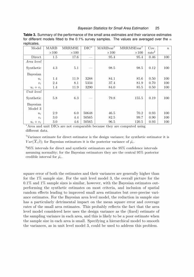
For this reduced sample, we have computed the MARB and MRRMSE forboth the small area estimates and their variance estimates for the area levelmodels and unit level models 3. These are shown in Table 3 together with theDICs and coverage rates of the 95% intervals. As expected, bias and mean


Table 3. Summary of the performance of the small area estimates and their variance estimatesfor different models fitted to the 0.1% survey samples. The values are averaged over the nreplicates.

Model MARB MRRMSE DIC∗ MARBvar† MRRMSEvar† Cov. n

×100 ×100 ×100 ×100 rate]

Direct 1.5 17.6 — 95.4 95.4 0.46 100

Area level

Synthetic 4.3 5.1 — 98.5 98.5 0.12 100

Bayesianui 1.4 11.9 3288 84.1 85.6 0.50 100vi 2.4 8.1 5334 37.4 81.9 0.70 100

ui + vi 1.4 11.9 3290 84.0 85.5 0.50 100

Unit level

Synthetic 5.8 6.3 — 79.8 155.5 0.19 100

BayesianModel 3

ui 2.9 6.0 50648 46.5 70.2 0.93 100vi 3.0 4.4 50565 82.5 99.7 0.90 100

ui + vi 3.0 4.6 50565 96.5 120.5 0.93 100∗Area and unit DICs are not comparable because they are computed usingdifferent data.

†Variance estimate for direct estimator is the design variance; for synthetic estimator it is

V ar(Xiβ); for Bayesian estimators it is the posterior variance of µi.

]95% intervals for direct and synthetic estimators are the 95% confidence intervalsassuming normality; for the Bayesian estimators they are the central 95% posteriorcredible interval for µi.

square error of both the estimates and their variances are generally higher thanfor the 1% sample size. For the unit level model 3, the overall picture for the0.1% and 1% sample sizes is similar, however, with the Bayesian estimates out-performing the synthetic estimates on most criteria, and inclusion of spatialrandom effects leading to improved small area estimates but over-precise vari-ance estimates. For the Bayesian area level model, the reduction in sample sizehas a particularly detrimental impact on the mean square error and coveragerates of the small area estimates. This probably reflects the fact that the arealevel model considered here uses the design variance as the (fixed) estimate ofthe sampling variance in each area, and this is likely to be a poor estimate whenthe sample size in each area is small. Specifying a hierarchical model to smooththe variances, as in unit level model 3, could be used to address this problem.


Regarding the convergence of the models, it seems to be better for unit levelmodel 3 than the other Bayesian models, probably because of the hierarchi-cal structure on the area level variances. In all cases, the model with bothrandom effects ui and vi showed that it is difficult to disentangle spatial andnon-spatial variation when data are sparse because of poor convergence andpossible confounding between the two effects; a phenomenon documented indisease mapping (Best et al., 2005).

6.4. Estimation in the absence of direct informationWe have extended our analysis to consider the case where there are only a fewareas in the sample. This is usually done in practice to reduce the survey costs.To be precise, we have considered a mock survey with only 100 municipalities,with a mean sample size of 166 (range 17 to 2910) for the 1% sample, andmean sample sizes of 17 (5 to 291) for the 0.1% sample. For the selection ofthe regions, we have created several socio-economic strata according to the areaaverage number of employed people per household and the proportion of headof household with tertiary studies. Each variable was divided in three intervals,which led to 9 strata. A sample size was assigned at each strata proportionallyto the number of municipalities that it contained, with the only constraint thatat least one municipality must be considered at each strata. Hence, the datais now made of the previous 100 survey data sets for each of the 1% and 0.1%samples but deleting the areas not included in the sampled regions. This meansthat the samples taken within each area are the same as before, so that MARBand MRRMSE can be directly compared.

When dealing with areas with missing observations it is important to con-sider carefully the missingness mechanism, because ignoring it can have animpact on the outcome (Little and Rubin, 2002). In our case, the probability ofbeing missing (i.e., not appearing in the sample) depends on a set of covariatesused to assign each area to a stratum which are assumed to be known. Hence,the missing data are Missing At Random (MAR) and, as discussed in Gelmanet al. (1995, page 205), the missingness mechanism can be ignored and the re-sults will not be affected because the covariates are included to estimate thearea level means.

Similar models to those used in the previous sections have been fitted to thesamples from the reduced set of areas. The results for area level model and unitlevel model 3 for both 1% and 0.1% samples are summarised in Table 4.

For in-sample areas, the bias and mean square error of the new small areaestimates are similar to those based on samples for the full set of areas, whilst, asexpected, estimates for off-sample areas have higher bias and mean square error.The notable exception is again the area-level model fitted to the 0.1% sample


Table 4. Summary of the performance of the small area estimates for selected models, inthe absence of direct information for some areas.

1% Survey Sample 0.1% Survey Sample

Model MARB MRRMSE Coverage MARB MRRMSE Coverage

×100 ×100 rate] ×100 ×100 rate]

(in/off) (in/off) (in/off) (in/off) (in/off) (in/off)

Area level

Synthetic 3.4/3.9 3.6/4.1 0.29/0.25 4.1/4.1 5.5/5.6 0.17/0.19

Bayesianui 1.8/3.7 3.0/3.9 0.92/0.44 1.2/3.5 11.3/5.1 0.46/0.71vi 1.9/3.4 2.9/3.9 0.90/0.86 1.2/3.3 11.4/7.8 0.48/0.99

ui + vi 1.8/3.4 2.9/3.9 0.91/0.85 1.2/3.5 11.4/5.4 0.46/0.85REGIONAL 1.8/3.4 2.9/3.9 0.90/0.64 1.2/3.5 11.3/5.1 0.46/0.76

Unit level

Synthetic 5.7/6.8 5.7/6.8 0.09/0.04 5.8/6.9 6.4/7.4 0.24/0.16

Bayesian Model 3ui 2.1/4.9 3.5/5.1 0.91/0.15 2.1/3.5 3.5/5.1 0.91/0.15vi 2.0/3.8 3.0/4.1 0.86/0.86 2.0/3.0 3.8/4.1 0.89/0.86

ui + vi 2.0/3.8 3.0/4.2 0.85/0.84 2.0/3.0 3.8/4.1 0.89/0.85REGIONAL 1.9/3.9 3.1/4.5 0.64/0.56 1.9/3.1 3.9/4.6 0.90/0.56

]95% intervals for synthetic estimators are the 95% confidence intervals assumingnormality; for the Bayesian estimators they are the central 95% posterior credibleinterval for µi.

size. Somewhat counter-intuitively, the mean square error in the off-sampleareas in this scenario is about half that of the in-sample areas. The explanationlies with the problem noted earlier, that treating the sample (design) variancein in-sample areas as fixed in the area level model is leading to poor estimateswhen data are sparse. The estimates for off-sample areas do not suffer fromthis problem, since there is no data in these areas and so their estimates aresimply predicted from the fitted model and do not depend on the observeddesign variance.

The average coverage rates for in-sample and off-sample areas have also beenincluded in the Table 4. In general, coverage rates for the in-sample areas aresimilar to, or slightly lower than, the full data case (again, the exception tothis is the area level model with 0.1% sample size, which has much lower thanexpected coverage). In off-sample areas, coverage is similar to that in in-sampleareas only for the models that include spatial random effects, and is lower forother models. This is because the unstructured random effects are set to zeroin these areas for identification, and so do not help to improve the small area


estimates in those areas.

6.5. Regional modelArea and unit level models based on the structure for µi in equation (16) havebeen computed to assess the value of borrowing information at a higher regionallevel when there are areas with missing observations. In general, these modelsperform similarly to the models with area (municipality) level spatial randomeffects, and better than the models with only unstructured random effects.This suggests that whilst inclusion of spatial random effects is important forimproving the small area estimates, the precise structure assumed for theserandom effects is less critical.

7. Discussion

In this paper we have described different Bayesian area and unit level modelsfor the estimation of variables in small areas by combining information fromsurvey data and other sources. We have studied the importance of taking intoaccount non-spatial and spatially correlated area level variation, and we havefound that by including random effects to model both these sources of variationthe small area estimates can be improved. These improvements are somewhatoffset by a tendency for spatial models to under-estimate the variances of theestimates, however. Despite this, we have shown that it becomes particularlyimportant to model spatial dependence when some areas have no direct surveyestimates, as information from nearby areas can be used to improve predictionin the off-sample areas.

When comparing area versus unit level models, the models performed sim-ilarly when using a 1% survey sample. However, when a 0.1% sample wasemployed, area level models had a smaller bias but were worse than unit levelmodels in terms of MRRMSE. We believe that this is due to the fact that thedirect estimators on which area level models rely are unbiased by design andhave a wide design variance in this case and are not very reliable. Smoothingthe within-area variances, as we did for the Bayesian unit level models, wouldhelp to address this problem.

Regarding unit level models, we considered three ways of modelling thewithin-area variance. Clearly, allowing for a different within-area variance foreach area improves the fitting. When there are sufficient data to estimate thewithin area variance with accuracy there is not much difference between Models2 and 3. However, the hierarchical structure on the area level variances as inModel 3 leads to better convergence of the MCMC simulations. In a moregeneral framework, a hierarchical structure based on covariates (for example,


linear regression) could be employed to model the different area level variances(see, for example, Gelman, 2006). Hence, we have shown the importance ofborrowing strength across areas when data are sparse not only to estimate thearea level means but also the area level variances.

In this work we have only considered models with a Normal response. Gen-eralised Linear Mixed Models can be used to deal with non-Normal variablesand the ideas presented here can still be applied. However, combining individ-ual and aggregated data is not so straightforward because in these models theresponse and the explanatory covariates are not linked linearly any more andso care is required to specify an appropriate aggregate form of the individual-level model. For example, as shown by Jackson et al. (2006), it is possible tosynthesise different sources of data, with different levels of aggregation when anappropriately specified model is used. Otherwise, a bias in the estimation ofthe coefficients of the covariates is introduced, which may bias the small areaestimates of the target variable as well. We intend to explore these ideas in thefuture and tackle their application to the estimation of area level counts andrates, such as the number of persons per household and rate of unemployment.

Areas can be classified to help inform policy issues by exploiting the resultsprovided by Bayesian inference. We have considered different approaches tothe ranking of areas. Accounting for the uncertainty of the estimates is crucialbecause when areas tend to be similar it will be difficult to separate low-rankedareas from the rest. Alternatively, the probability of being among the q% lowestranked areas can be used instead, for some suitable quantile, q. We have shownthat choosing more extreme quantiles (e.g. the lowest ranked area rather thanthe bottom 10% or 20%) reduces uncertainty about the ranks due to samplingvariation. However, it is still difficult to confidently identify all but the mostextreme ranked areas.

When some areas are not included in the survey, it is still possible to pro-vide estimates for those areas by relying on the fitted Bayesian models (usingin-sample areas) and their spatial correlation to off-sample areas. Area levelcovariates are still required in all areas to compute the small area estimates. Asexpected, these estimates are less accurate than in the case with survey data inall areas but, despite the loss of performance, the results are still reasonable andhave lower bias and better coverage than traditional synthetic estimates. Whendata are very sparse, spatial random effects can be incorporated at a regionallevel, so that larger-scale spatial patterns are modelled. This can help to copewith large amounts of areas with no direct observations and provide reliableresults.


8. Acknowledgements

We would like to thank ONS for providing access to the Swedish data, whichwere originally provided by Statistics Sweden. This work was carried out as partof the Imperial College BIAS node of the ESRC National Centre for ResearchMethods (grant numbers RES-576-25-5003 and RES-576-25-0015). We wouldalso want to thank the associate editor and two anonymous referees whosecomments have helped to improve the quality of this paper.

References

Arora, V. and P. Lahiri (1997). On the superiority of the Bayesian method overthe BLUP in Small Area estimation problems. Statistica Sinica 7, 1053–1063.

Arora, V., P. Lahiri, and K. Mukherjee (1997). Empirical Bayes estimationof finite population means from complex surveys. Journal of the AmericanStatistical Association 92 (440), 1555–1562.

Banerjee, S., B. P. Carlin, and A. E. Gelfand (2004). Hierarchical Modeling andAnalysis for Spatial Data. Chapman & Hall/CRC, Boca Raton, Florida.

Barton, J., R. Chung, D. Donaldson, J. Shome, J. Snow, E. Whiting, andM. Willitts (Eds.) (2007). Family Resources Survey. United Kingdom 2005-2006. National Statistics, Department for Work and Pensions (UK).

Battese, G. E., R. M. Harter, and W. A. Fuller (1988). County crop areasusing survey data and satellite data. Journal of the American StatisticalAssociation 83 (401), 28–36.

Bell, W. R. (2004). A Bayesian approach to recognizing Statistical Uncertaintyin ranked Survey Estimates. U.S. Census Bureau, Census Advisory Commit-tee of Prefessional Association Meetings. April 22-23, 2004.

Besag, J., J. C. York, and A. Mollie (1991). Bayesian image restoration, withtwo applications in spatial statistics. Annals of the Institute of StatisticalMathematics 43, 1–59.

Best, N., S. Richardson, and A. Thomson (2005). A comparison of Bayesianspatial models for disease mapping. Statistical Methods in Medical Re-search 14 (1), 35–59.

Breslow, N. E. and D. G. Clayton (1993). Approximate inference in generalizedlinear models. Journal of the American Statistical Association 88 (421), 9–25.


Cochran, W. G. (1977). Sampling Techniques (3rd ed.). John Wiley & Sons,Inc., New York.

Conlon, E. M. and T. A. Louis (1999). Addressing multiple goals in evaluat-ing region-specific risk using Bayesian methods. In A. Lawson, A. Biggeri,D. Bohning, E. Lesaffre, J.-F. Viel, and R. Bertollini (Eds.), Disease Mappingand Risk Assessment for Public Health, pp. 31–47. Wiley.

Datta, G. S. and M. Ghosh (1991). Bayesian prediction in linear models: Appli-cations to small area estimation. The Annals of Statistics 19 (4), 1748–1770.

Diggle, P., R. Moyeed, B. Rowlingson, and M. Thomson (2002). Childhoodmalaria in the Gambia: a case-stuy in model-based geostatistics. AppliedStatistics 51, 493–506.

Diggle, P., J. Tawn, and R. Moyeed (1998). Model-based geostatistics. AppliedStatistics 47, 299–350.

Eberley, L. E. and B. P. Carlin (2000). Identifiability and convergence issues forMarkov Chain Monte Carlo fitting of spatial models. Statistics in Medicine 19,2279–2294.

EURAREA Consortium (2004). Project reference volume. Technical report,EURAREA Consortium.

Fay, R. E. and R. A. Herriot (1979). Estimates of income for small places:An application of James-Stein procedures to census data. Journal of theAmerican Statistical Association 74 (366), 269–277.

Gelman, A. (2006). Prior distributions for variance parameters in hierarchicalmodels (Comment on article by Browne and Draper). Bayesian Analysis 31,515 – 533.

Gelman, A., J. B. Carlin, H. S. Stern, and D. B. Rubin (1995). Bayesian DataAnalysis. Chapman & Hall/CRC, Boca Raton, Florida.

Ghosh, M. (1992). Constrained Bayes estimation with applications. Journal ofthe American Statistical Association 87 (418), 533–540.

Ghosh, M., K. Natarajan, T. W. F. Stroud, and B. P. Carlin (1998). Generalizedlinear models for small-area estimation. Journal of the American StatisticalAssociation 93 (441), 273–282.

Gilks, W. R., S. Richardson, and D. J. Spiegelhalter (Eds.) (1995). MarkovChain Monter Carlo in Practice. Chapman & Hall/CRC, Boca Raton,Florida.


Goldstein, H. and D. J. Spiegelhalter (1996). League tables and their limi-tations: Statistical issues in comparisons of institutional performance (withdiscussion). Journal of the Royal Statistical Society, Series A 159 (3), 385–443.

Gonzalez, M. E. (1973). Use and evaluation of synthetic estimators. In Pro-ceedings of the Social Statistics Section, pp. 33–36. American Statistical As-sociation, Washington, D.C.

Greenland, S. and J. Robins (1994). Ecologic studies–biases, misconceptions,and counterexamples. American Journal of Epidemiology 139 (8), 747–760.

Heady, P., P. Clarke, and others (2003). Small Area Estimation Project Report.Technical report, Office for National Statistics, United Kingdom.

Hills, J. (2004). Inequality and the State. Oxford University Press.

Jackson, C., N. Best, and S. Richardson (2006). Improving ecological inferenceusing individual-level data. Statistics in Medicine 25 (12), 2136–2159.

Jiang, J. and P. Lahiri (2006). Mixed model prediction and small area estima-tion. Test 15 (1), 1–96.

Kleffe, J. and J. N. K. Rao (1992). Estimation of mean square error of empir-ical bests linear unbiased predictors under a random variance linear model.Journal of Multivariate Analysis 43, 1–15.

Lahiri, P. (1990). “Adjusted” Bayes and Empirical Bayes estimation in finitepopulation sampling. Sankhya, Series B 52 (1), 50–66.

LeSage, J. P. and R. K. Pace (2004). Models for spatially dependent missingdata. Journal of Real Estate Finance and Economics 29 (2), 233–254.

Lin, R., T. A. Louis, S. M. Paddock, and G. Ridgeway (2006). Loss functionbased ranking in two-stage hierarchical models. Bayesian Analysis 1 (4), 915–946.

Lin, R., T. A. Louis, S. M. Paddock, and G. Ridgeway (2009). Ranking US-RDS provider specific SMRs from 1998-2001. Health Services and OutcomesResearch Methodology 9, 22–38.

Little, R. J. and D. B. Rubin (2002). Statistical Analysis with Missing Data.John Wiley & Sons, Inc., Hoboken, New Jersey.


Louis, T. A. (1984). Estimating a population of parameter values using Bayesand Empirical Bayes methods. Journal of the American Statistical Associa-tion 79 (386), 393–398.

Morris, C. N. and C. L. Christiansen (1996). Hierarchical model for rankingand for identifying extremes, with applications (with discussion). In J. M.Bernardo, J. O. Berger, A. P. Dawid, and A. F. M. Smith (Eds.), BayesianStatistics 5, pp. 277–296. Oxford Unviersity Press.

Normand, S. L., M. E. Glickman, and C. Gatsonis (1997). Statistical methodsfor profiling providers of medical care: issues and applications. Journal of theAmerican Statistical Association 92, 803–814.

Paddock, S. M., G. Ridgeway, R. Lin, and T. A. Louis (2006). Flexible distribu-tions for triple-goal estimates in two-stage hierarchical models. ComputationalStatistics and Data Analysis 50, 3243–3262.

Petrucci, A. and N. Salvati (2005). Small area estimation for spatial correla-tion in watershed erosion assessment. Journal of Agricultural, Biological &Environmental Statistics 11 (2), 169–182.

Rao, J. N. K. (2003). Small Area Estimation. John Wiley & Sons, Inc., Hoboken,New Jersey.

Robinson, G. K. (1991). That BLUP is a good thing: the estimation of randomeffects (with discussion). Statistical Science 6, 15–51.

Saei, A. and R. Chambers (2005). Working paper M05/03: Empirical Best Lin-ear Unbiased Prediction for out of sample areas. Technical report, Southamp-ton Statistical Sciences Research Institute, University of Southampton.

Sarndal, C.-E., B. Swensson, and J. Wretman (1992). Model Assisted SurveySampling. Springer-Verlag Inc., New York.

Shen, W. and T. A. Louis (1998). Triple-goal estimates in two-stage hierarchicalmodels. Journal of the Royal Statistical Society, Series B 60 (2), 455–471.

Shen, W. and T. A. Louis (2000). Triple-goal estimates for disease mapping.Statistics in Medicine 19, 2295–2308.

Singh, B. B., G. K. Shukla, and D. Kundu (2005). Spatio-temporal models insmall area estimation. Survey Methodology 31 (2), 183–196.

Spiegelhalter, D. J., N. G. Best, B. P. Carlin, and A. van der Linde (2002).Bayesian measures of model complexity and fit (with discussion). J. R. Statist.Soc. B 64, 583–639.


Spjøtvoll, E. and I. Thomsen (1987). Applications of some Empricial Bayesmethods to Small Area Estimation. Bulletin of the International StatisticalInstitute 46 (2), 435–449.

Staubach, C., V. Schmid, L. Knorr-Held, and M. Ziller (2002). A Bayesianmodel for spatial wildlife disease prevalence data. Preventive VeterinaryMedicine 56 (1), 75–87.


A. Full conditional distributions for CAR specification with missing ob-servations

Let us assume that we have an area level model and that we have data fromthe first l areas, i.e., we have the values of direct estimates and their samplingvariances for these areas. In this context, s = {1, . . . , l} and s = {l+ 1, . . . ,m}.

The full conditionals to be used in Gibbs Sampling for this model are:

Π(α, β| . . .) = N(

(XTV −1X)−1X

TV −1(Y − v), (X

TV −1X)−1

)where Y = (Y 1, . . . , Y l)

T , v = (v1, . . . , vl)T , V = diag(V 2

1 , . . . , V2l ) and

XT

=

1 . . . 1

X1 . . . X l

Π(vi|...) ∝ exp{−1

σ2i

(Y i − α− βXi − vi)2 +−1

σ2v

ni(vi − vi)2}, i ∈ s

Π(vj |...) ∝ exp{−1

σ2v

nj(vj − vj)2}, j ∈ s

where ni and nj represent the number of neighbours of areas i and j, respec-tively.

Π(σ2v|...) = Ga−1(ε+

n

2, ε+

1

2

∑k∼l

(vk − vl)2)

Note that the full conditional for each vi depends directly on observed dataand its neighbours, whilst vj only depends on its neighbours through vj andnot directly on the observed data. Furthermore, α and β are only informed bythe data from the areas included in the survey, as we would expect.


●

●

●

●

●

●

●

●

●

●

●

●

●

●

●

●

●

●

●

●

●

●

●

●

●

●

●

●

●

●

●

●

●

●

●

●

●

●

●

●

●

●

●

●

●

●

●

●●

●

●

●

●

●

●

●

●

●

●

●

●●

●

●

●

●

●●

●

●

●

●

●

●

●

●

●

●

●

●

●

●

●

●

●

●

●

●

●

●

●

●

●

●

●

●

●●

●

●

●

●

●

●

●

●

●

●

●

●

●

●

●

●

●

●

●

●

●

●

●●

●

●

●

●

●

●

●

●●

●

●

●

●

●

●

●

●

●

●

●

●●

●●

●

●●

●

●

●

●

●

●

●●

●

●

●

●

●

●●●●

●

●●

●

●

●

●

●

●●●

●

●●

●

●

●

●

●●

●

●

●

●

●

●

●●

●

●

●

●●●

●

●

●

●

●

●●●

●

●●●●●●

●

●●

●

●

●

●

●

●●●●●●●●●

●

●●●●●

●

●●●●●

●

●●●

●

●●●●●●●●●●●●●●●●●●●●●●●●●●●●●●●●●●●

0 50 100 150 200 250

0.0

0.2

0.4

0.6

0.8

1.0

Prob. in poorest 20% of areas

True Area Rank

Pro

babi

lity

●

●

●

●

●

●

●

●

●

●

●

●

●

●

●

●

●

●

●

●

●

●

●

●

●

●

●

●

●

●

●

●

●

●

●

●

●

●

●

●

●

●

●

●

●

●

●

●●

●

●

●

●

●

●

●

●

●

●

●

●●

●

●

●

●

●●

●

●

●

●

●

●

●

●

●

●

●

●

●

●

●

●

●

●

●

●

●

●

●

●

●

●

●

●

●●

●

●

●

●

●

●

●

●

●

●

●

●

●

●

●

●

●

●

●

●

●

●

●●

●

●

●

●

●

●

●

●●

●

●

●

●

●

●

●

●

●

●

●

●●

●●

●

●●

●

●

●

●

●

●

●●

●

●

●

●

●

●●●●

●

●●

●

●

●

●

●

●●●

●

●●

●

●

●

●

●●

●

●

●

●

●

●

●●

●

●

●

●●●

●

●

●

●

●

●●●

●

●●●●●●

●

●●

●

●

●

●

●

●●●●●●●●●

●

●●●●●

●

●●●●●

●

●●●

●

●●●●●●●●●●●●●●●●●●●●●●●●●●●●●●●●●●●

●

●

●

●

●

●

●

●

●

●●

●

●●

●

●●

●

●

●

●

●●

●

●

●

●

●

●

●

●

●

●

●●

●

●

●

●

●●

●●

●

●

●

●

●

●

●

●

●

●

●●●

●

●

●

●

●

●

●

●

●

●

●●

●

●

●

●

●

●

●

●

●

●

●

●

●

●

●●

●

●

●

●

●

●●

●

●

●

●

●

●

●●

●

●●

●

●

●

●

●●

●

●

●

●

●●

●

●

●●

●●

●●

●

●

●

●

●

●

●

●

●

●

●●●●

●

●

●

●

●

●

●

●

●

●

●

●

●

●●

●

●

●

●

●

●

●

●

●

●

●

●

●●

●

●●

●

●

●

●

●

●

●

●

●

●

●

●

●

●

●

●

●

●

●

●

●

●

●

●

●

●●

●

●

●●●●●

●

●

●

●●●

●

●

●●●●●

●

●●●●

●

●

●●

●

●●

●

●

●

●

●

●●●●

●●

●

●●●●●●●●●

●

●

●●●●●●●●●●●●●●●●●●●●●●●●●●●●●●●●●●

0 50 100 150 200 250

0.0

0.2

0.4

0.6

0.8

1.0


True Area Rank

Mea

n of

the

post

erio

r pr

obab

ilitie

s

●

●

●

●

●

●

●

●

●

●●

●

●●

●

●●

●

●

●

●

●●

●

●

●

●

●

●

●

●

●

●

●●

●

●

●

●

●●

●●

●

●

●

●

●

●

●

●

●

●

●●●

●

●

●

●

●

●

●

●

●

●

●●

●

●

●

●

●

●

●

●

●

●

●

●

●

●

●●

●

●

●

●

●

●●

●

●

●

●

●

●

●●

●

●●

●

●

●

●

●●

●

●

●

●

●●

●

●

●●

●●

●●

●

●

●

●

●

●

●

●

●

●

●●●●

●

●

●

●

●

●

●

●

●

●

●

●

●

●●

●

●

●

●

●

●

●

●

●

●

●

●

●●

●

●●

●

●

●

●

●

●

●

●

●

●

●

●

●

●

●

●

●

●

●

●

●

●

●

●

●

●●

●

●

●●●●●

●

●

●

●●●

●

●

●●●●●

●

●●●●

●

●

●●

●

●●

●

●

●

●

●

●●●●

●●

●

●●●●●●●●●

●

●

●●●●●●●●●●●●●●●●●●●●●●●●●●●●●●●●●●

●

●●●●

●●●●

●●

●●●●●●

●

●●●●●●

●●●

●●●●

●●●●●

●●

●

●●●●

●●

●●

●●●●

●

●●●●●

●●

●●

●

●

●●

●

●●●

●

●●●●●●

●

●

●●

●●●●●●●

●●●●

●

●

●

●●●●●●

●●

●●●

●

●●●

●

●●●●●

●

●●●●●●

●

●●●●●●

●●●●●●●

●●

●●

●●●

●

●

●●

●●●●●

●

●●

●●

●●●●

●●

●●●●●

●●

●

●

●●●●

●●●●

●

●

●●●

●●●●●

●

●

●●●●●

●

●●

●●●●●●●

●●●●●●●●

●●

●

●●●●●

●●●●●●●●●

●●●●●●●●●●●●●●●●●●●●●●●●●●●●●●●

●●●●●●

●●●●●●

●●●●●●

●●●

0 50 100 150 200 250

050

100

150

200

250

Mean of the ranks of the posterior prob. (in poorest 20% of areas)

True Area Rank

Ran

k

●

●

●

●

●

●

●

●

●

●

●

●

●

●

●

●

●

●

●

●

●

●

●

●

●

●

●

●

●

●

●

●

●

●

●

●

●

●

●

●

●

●

●

●

●

●

●

●●

●

●

●

●

●

●

●

●

●

●

●

●

●

●

●

●

●

●●

●

●

●

●

●

●

●

●

●

●

●

●

●

●

●●

●

●

●

●●

●

●

●

●

●

●

●

●●●

●

●

●

●

●

●

●

●

●

●

●

●

●

●●●

●

●

●●

●●●●

●

●

●

●

●

●●●

●

●

●

●

●

●

●

●

●●●●●

●●●

●●●●●

●

●

●

●●

●

●

●

●

●

●●●●

●

●●●●●●

●

●●●●●●●

●

●

●

●●

●

●

●

●

●

●

●

●●●●●●●

●

●

●

●●●●●

●

●●●●●●●●●

●

●

●●

●●●●●●●●●●

●

●●●●●

●

●●●●●●●●●●●●●●●●●●●●●●●●●●●●●●●●●●●●●●●●●●●●●

0 50 100 150 200 250

0.0

0.2

0.4

0.6

0.8

1.0


True Area Rank

Pro

babi

lity

●

●

●

●

●

●

●

●

●

●

●

●

●

●

●

●

●

●

●

●

●

●

●

●

●

●

●

●

●

●

●

●

●

●

●

●

●

●

●

●

●

●

●

●

●

●

●

●●

●

●

●

●

●

●

●

●

●

●

●

●

●

●

●

●

●

●●

●

●

●

●

●

●

●

●

●

●

●

●

●

●

●●

●

●

●

●●

●

●

●

●

●

●

●

●●●

●

●

●

●

●

●

●

●

●

●

●

●

●

●●●

●

●

●●

●●●●

●

●

●

●

●

●●●

●

●

●

●

●

●

●

●

●●●●●

●●●

●●●●●

●

●

●

●●

●

●

●

●

●

●●●●

●

●●●●●●

●

●●●●●●●

●

●

●

●●

●

●

●

●

●

●

●

●●●●●●●

●

●

●

●●●●●

●

●●●●●●●●●

●

●

●●

●●●●●●●●●●

●

●●●●●

●

●●●●●●●●●●●●●●●●●●●●●●●●●●●●●●●●●●●●●●●●●●●●●

●

●

●

●

●

●

●

●

●

●

●

●

●●

●

●

●●

●

●

●

●

●

●

●

●

●●

●

●

●

●

●

●●

●

●

●

●

●●

●●

●

●

●

●●

●

●

●

●

●

●●●

●

●

●●

●

●

●

●

●

●

●●●

●●

●

●

●

●

●

●

●

●

●

●

●

●

●

●

●

●

●●

●

●

●

●

●

●

●

●●●●

●●●

●

●

●

●●●

●

●

●

●●

●

●

●●

●●

●●

●

●

●

●

●

●

●

●

●

●

●●●●

●

●

●

●

●●

●

●

●

●●

●

●

●●●

●

●

●●

●

●

●

●●

●

●

●●●

●●

●

●

●

●

●

●

●●

●

●●●

●

●

●

●

●●●●●

●

●

●

●

●●

●●●●●●●

●

●

●

●●●

●

●

●●●●●●●●●●

●

●

●●

●

●●●●●●

●

●●●●●●●●●●●●●●●●●

●●●●●●●●●●●●●●●●●●●●●●●●●●●●●●●●●●●

0 50 100 150 200 250

0.0

0.2

0.4

0.6

0.8

1.0


True Area Rank

Mea

n of

the

post

erio

r pr

obab

ilitie

s

●

●

●

●

●

●

●

●

●

●

●

●

●●

●

●

●●

●

●

●

●

●

●

●

●

●●

●

●

●

●

●

●●

●

●

●

●

●●

●●

●

●

●

●●

●

●

●

●

●

●●●

●

●

●●

●

●

●

●

●

●

●●●

●●

●

●

●

●

●

●

●

●

●

●

●

●

●

●

●

●

●●

●

●

●

●

●

●

●

●●●●

●●●

●

●

●

●●●

●

●

●

●●

●

●

●●

●●

●●

●

●

●

●

●

●

●

●

●

●

●●●●

●

●

●

●

●●

●

●

●

●●

●

●

●●●

●

●

●●

●

●

●

●●

●

●

●●●

●●

●

●

●

●

●

●

●●

●

●●●

●

●

●

●

●●●●●

●

●

●

●

●●

●●●●●●●

●

●

●

●●●

●

●

●●●●●●●●●●

●

●

●●

●

●●●●●●

●

●●●●●●●●●●●●●●●●●

●●●●●●●●●●●●●●●●●●●●●●●●●●●●●●●●●●●

●

●●●●●

●●●

●●●●●●●

●●

●●

●●

●

●●

●

●

●

●

●●●●●●●●●●●

●●●

●●

●

●

●

●

●

●●●●●

●

●●●

●

●●●●●●

●

●●

●

●

●

●

●●●●●

●●

●

●●●●

●●

●

●●

●●

●

●●●●●

●

●

●

●

●●●●●●

●●●●●●

●

●●●●●●●

●●●

●

●

●

●●●

●●

●

●

●●●●●

●

●●●●

●●

●

●

●

●●●●●●●●●●●●

●●●●

●

●

●●

●

●

●

●

●●●●●

●●

●

●●

●

●●●

●

●

●

●●●●●●

●●●●

●●●●●●●●

●●●●●●●●●●●●●●●●●●●●●●●●●●●●●●●●●●●●●●

●●●●●●●●

●●●●●

●●●●●●

●●●●●●

●●●●●●

●●●●●●

0 50 100 150 200 250

050

100

150

200

250

Mean of the ranks of the posterior prob. (in poorest 10% of areas)

True Area Rank

Ran

k

●●●●

●

●●●

●

●●●●●●●●●●●●●

●

●●

●

●●●●●

●

●●●●●●●●●

●●●●●●●●●●

●●●●●●●●●●●●●●●●●●●●●●●●●●●●●●●●●●●●●●●

●

●●

●

●●●●●●●●●●●●●●●●●●

●●●●●●●●●●●●●●●●●●●●●●●●●●●●●●●●●●●●●●●●●●●●●●●●●●●●●●●●●●●●●●●●●●●●●●●●●●●●●●●●●●●●●●●●●●●●●●●●●●●●●●●●●●●●●●●●●●●●●●●●●●●●●●●●●●●●●●●●●●●●●●●●●●●●●●●●●●●●●●●●●●●●●●●●●●●●

0 50 100 150 200 250

0.0

0.2

0.4

0.6

0.8

1.0

Prob. poorest area

True Area Rank

Pro

babi

lity

●●●●

●

●●●

●

●●●●●●●●●●●●●

●

●●

●

●●●●●

●

●●●●●●●●●

●●●●●●●●●●

●●●●●●●●●●●●●●●●●●●●●●●●●●●●●●●●●●●●●●●

●

●●

●

●●●●●●●●●●●●●●●●●●

●●●●●●●●●●●●●●●●●●●●●●●●●●●●●●●●●●●●●●●●●●●●●●●●●●●●●●●●●●●●●●●●●●●●●●●●●●●●●●●●●●●●●●●●●●●●●●●●●●●●●●●●●●●●●●●●●●●●●●●●●●●●●●●●●●●●●●●●●●●●●●●●●●●●●●●●●●●●●●●●●●●●●●●●●●●● ●

●●●

●

●●

●

●

●●●●●●

●●●●●●

●

●

●●●●●●●●●●●●●●●

●

●●●●●●●●●●●●●●●●●●●●●

●●●●●●●●●●●●●●●●●●●●●●●●●●●●●●●

●

●●●●●●●●●●●●●●●●●●●●●●●●●●●●●●●●●●●●●●●●●●●●●●●●●●●●●●●●●●●●●●●●●●●●●●●●●●●●●●●●●●●●●●●●●●●●●●●●●●●●●●●●●●●●●●●●●●●●●●●●●●●●●●●●●●●●●●●●●●●●●●●●●●●●●●●●●●●●●●●●●●●●●●●●●●●●●●●●●●●●●●●●●●●●●●●●

0 50 100 150 200 250

0.0

0.2

0.4

0.6

0.8

1.0

Prob. poorest area

True Area Rank

Mea

n of

the

post

erio

r pr

obab

ilitie

s

●

●●●

●

●●

●

●

●●●●●●

●●●●●●

●

●

●●●●●●●●●●●●●●●

●

●●●●●●●●●●●●●●●●●●●●●

●●●●●●●●●●●●●●●●●●●●●●●●●●●●●●●

●

●●●●●●●●●●●●●●●●●●●●●●●●●●●●●●●●●●●●●●●●●●●●●●●●●●●●●●●●●●●●●●●●●●●●●●●●●●●●●●●●●●●●●●●●●●●●●●●●●●●●●●●●●●●●●●●●●●●●●●●●●●●●●●●●●●●●●●●●●●●●●●●●●●●●●●●●●●●●●●●●●●●●●●●●●●●●●●●●●●●●●●●●●●●●●●●●

●●●

●●●●●●●

●●

●●●●

●●●●

●●●●

●

●●●

●

●●

●●●●

●●●●●

●●●●●

●●●●●

●

●●●

●●

●

●●

●●●●●●●●●

●●

●●●●●●

●●●●

●●

●●●●

●●●

●●

●●●●●●●

●●●●●●●●●●

●●●●●●●●●●●●●●●●●●●●●●●●●●●●●●●

●●●●●●●

●●●●●●●●●●●●●

●●●●●

●●●●●●

●●●●●●

●●●●●

●●●●●●

●●●●●

●●●●●●

●●●●●●

●●●●●●●

●●●●●●

●●●●●●

●●●●●●

●●●●●●

●●●●●●

●●●●●●

●●●●●●

●●●●●●

●●●●●●

●●●●●●

●●●●●●

●●●●●●

●

0 50 100 150 200 250

050

100

150

200

250

Rank of the mean posterior prob. (poorest area)

True Area Rank

Ran

k

●

●

●

●

●

●●

●

●

●●●●

●

●

●

●●

●●●●

●

●

●

●

●

●

●●●

●

●●

●

●●●●

●●

●

●

●

●

●

●●●●●

●

●

●

●●●

●●●●●●●

●

●●●

●●●

●

●●●●●●●●●●●●●●

●

●●●

●

●

●

●

●●●●●●●●●●●●●●●●●

●

●●●●●●●●●●●

●●●●●●●●●●●●●

●●●●●●●●●●●●●●●●●●●●●●

●

●●●●●●●●●●●●●●●●●●●●●●●●●●●●●●●●●●●●●●●●●●●●●●●●●●●●●●●●●●●●●●●●●●●●●●●●●●●●●●●●●●●●●●●●●●●●●●●●●●●●●●●●●●●●●●●●●●●●●●●●●●●●●

0 50 100 150 200 250

0.0

0.2

0.4

0.6

0.8

1.0

Prob. Income < 1050

True Area Rank

Pro

babi

lity

●

●

●

●

●

●●

●

●

●●●●

●

●

●

●●

●●●●

●

●

●

●

●

●

●●●

●

●●

●

●●●●

●●

●

●

●

●

●

●●●●●

●

●

●

●●●

●●●●●●●

●

●●●

●●●

●

●●●●●●●●●●●●●●

●

●●●

●

●

●

●

●●●●●●●●●●●●●●●●●

●

●●●●●●●●●●●

●●●●●●●●●●●●●

●●●●●●●●●●●●●●●●●●●●●●

●

●●●●●●●●●●●●●●●●●●●●●●●●●●●●●●●●●●●●●●●●●●●●●●●●●●●●●●●●●●●●●●●●●●●●●●●●●●●●●●●●●●●●●●●●●●●●●●●●●●●●●●●●●●●●●●●●●●●●●●●●●●●●● ●

●

●

●

●

●●

●

●

●

●

●

●●●

●●●

●●

●

●

●

●●●●

●●●

●

●

●●●●●

●

●

●●●●●

●●●●●●

●

●

●

●●●●●●●

●●

●●●●

●●●●●

●

●

●

●●●●

●●

●●●

●

●

●●●●●●

●

●●●●●●●●●●●

●

●●●●●●●●●●●●●●●●●●●●●●

●●●●●●●●●●

●●●●●●●●

●●●●●●●●●●●●●●

●●●●●●●●●●●●●●●●●●●●●●●

●●●●●●●●●●●●●●●●●●●●●

●●●●●●●●●●●●●●●●●●●●●●●●●●●●●●●●●●●●●●●●●●●●●●●●●●●●●●●●●●●●●●●●●●●●●●●●●●●●●●●●●●

0 50 100 150 200 250

0.0

0.2

0.4

0.6

0.8

1.0

Prob. Income < 1050

True Area Rank

Mea

n of

the

post

erio

r pr

obab

ilitie

s

●

●

●

●

●

●●

●

●

●

●

●

●●●

●●●

●●

●

●

●

●●●●

●●●

●

●

●●●●●

●

●

●●●●●

●●●●●●

●

●

●

●●●●●●●

●●

●●●●

●●●●●

●

●

●

●●●●

●●

●●●

●

●

●●●●●●

●

●●●●●●●●●●●

●

●●●●●●●●●●●●●●●●●●●●●●

●●●●●●●●●●

●●●●●●●●

●●●●●●●●●●●●●●

●●●●●●●●●●●●●●●●●●●●●●●

●●●●●●●●●●●●●●●●●●●●●

●●●●●●●●●●●●●●●●●●●●●●●●●●●●●●●●●●●●●●●●●●●●●●●●●●●●●●●●●●●●●●●●●●●●●●●●●●●●●●●●●●

●●●

●●

●●●●

●●

●●

●●●●

●

●●●

●●●●●●●●

●●●

●●●

●●●●

●●●●●

●

●

●

●●●●●●

●●

●●

●

●●●●●●

●

●

●●

●●

●●●

●

●

●

●

●●●

●

●●

●

●●

●●●

●

●●●●●●

●

●

●●●●

●●●●●

●●●●●●●●●●●●●●

●●●

●●●●

●●●●●

●●●●●

●●●●●●●

●●●●●

●●●●●●●●

●●●●●●

●●●●●●●●●●●●●●●●●●●●●●●●●●●●●●●●●●●●●●●●●●●

●●●●●●●●●

●●●●●●

●●●●●●●

●●●●●●

●●●●●●

●●●●●●

●●●●●●

●●●●●●

●●●●●●

●●●●●●

●●●●●●

●●●●●●

●

0 50 100 150 200 250

050

100

150

200

250

Rank of the mean posterior prob. (of Income < 1050)

True Area Rank

Ran

k

Figure 2. Ranking of the areas according to four different criteria. Left column showsthe exceedence or percentile probabilities for each area for a randomly selected dataset; middle column shows the mean of these probabilities across all datasets; right col-umn shows mean of the rank of these probabilities across datasets. Grey dashed linesare 95% ’sampling intervals’ and show the uncertainty about the replication variabilityfor the probabilities and ranks across the survey samples.

bayesian statistics for small area estimation - bias project · bayesian statistics for small area...

Documents