Bayesian Subset Simulation

— a kriging-based subset simulation algorithm forthe estimation of small probabilities of failure —

Ling Li, Julien Bect, Emmanuel Vazquez

Supelec, France

PSAM11-ESREL12Helsinki, June 26, 2012

A classical problem in (probabilistic) reliability. . . (1/2)

❍ Consider a system subject to uncertainties,

◮ aleatory and/or epistemic,

◮ represented by a random vector X ∼ PX

where PX is a probability measure on X ⊂ Rd .

A classical problem in (probabilistic) reliability. . . (1/2)

❍ Consider a system subject to uncertainties,

◮ aleatory and/or epistemic,

◮ represented by a random vector X ∼ PX

where PX is a probability measure on X ⊂ Rd .

❍ Assume that the system fails when f (X ) > u

◮ f : X → R is a cost function,

◮ u ∈ R is the critical level.

❍ x 7→ u − f (x) is sometimes called the “limit state function”

A classical problem in (probabilistic) reliability. . . (2/2)

❍ Define the failure region

Γ = {x ∈ X : f (x) > u}.

❍ The probability of failure is

α = PX{Γ} =

∫

X

1f >u dPX

f(x)

PX

α

Γ

x

u

Figure: A 1d illustration

A classical problem in (probabilistic) reliability. . . (2/2)

❍ Define the failure region

Γ = {x ∈ X : f (x) > u}.

❍ The probability of failure is

α = PX{Γ} =

∫

X

1f >u dPX

f(x)

PX

α

Γ

x

u

Figure: A 1d illustration

A fundamental numerical problem in reliability analysis

How to estimate α using a computer program that can providef (x) for any given x ∈ X ?

The venerable Monte Carlo method

❍ The Monte Carlo (MC) estimator

α̂MC =1

m

m∑

i=1

1f (Xi )>u with X1, . . . , Xm

iid∼ PX

has a coefficient of variation given by

δ =

√

1 − α

αm≈ 1√

αm.

The venerable Monte Carlo method

❍ The Monte Carlo (MC) estimator

α̂MC =1

m

m∑

i=1

1f (Xi )>u with X1, . . . , Xm

iid∼ PX

has a coefficient of variation given by

δ =

√

1 − α

αm≈ 1√

αm.

❍ Computation time for a given δ ?

m ≈ 1

δ2 α⇒ τMC ≈ τ0

δ2 α

Ex: with δ = 50%, α = 10−5, τ0 = 5 min, τMC ≈ 4 years.

A short and selective review of existing techniques

❍ The MC estimator is impractical when

◮ either f is expensive to evaluate (i.e., τ0 is large),

◮ or Γ is a rare event under PX (i.e., α is small).

A short and selective review of existing techniques

❍ The MC estimator is impractical when

◮ either f is expensive to evaluate (i.e., τ0 is large),

◮ or Γ is a rare event under PX (i.e., α is small).

❍ Approximation techniques (and related adaptive samplingschemes) address the first issue.

◮ parametric: FORM/SORM, polynomial RSM, . . .

◮ non-parametric: kriging (Gaussian processes), SVM, . . .

A short and selective review of existing techniques

❍ The MC estimator is impractical when

◮ either f is expensive to evaluate (i.e., τ0 is large),

◮ or Γ is a rare event under PX (i.e., α is small).

❍ Approximation techniques (and related adaptive samplingschemes) address the first issue.

◮ parametric: FORM/SORM, polynomial RSM, . . .

◮ non-parametric: kriging (Gaussian processes), SVM, . . .

❍ Variance reduction techniques (e.g., importance sampling)address the second issue.

◮ Subset simulation (Au & Beck, 2001) is especially

appropriate for very small α, since δ ∝√

| log α|/√m.

What if I have an expensive f and a small α ? (1/2)

❍ Some parametric approximation techniques (e.g.,FORM/SORM) can be still be used. . .

◮ strong assumption ⇒ “structural” error that cannot bereduced by adding more samples.

What if I have an expensive f and a small α ? (1/2)

❍ Some parametric approximation techniques (e.g.,FORM/SORM) can be still be used. . .

◮ strong assumption ⇒ “structural” error that cannot bereduced by adding more samples.

❍ Contribution of this paper: Bayesian Subset Simulation (BSS)

◮ Bayesian: uses a Gaussian process prior on f (kriging)◮ flexibility of a non-parametric approach,◮ framework to design efficient adaptive sampling schemes.

◮ generalizes subset simulation◮ in the framework of Sequential Monte Carlo (SMC)

methods (Del Moral et al, 2006).

What if I have an expensive f and a small α ? (2/2)

❍ Some recent related work

◮ V. Dubourg, F. Deheeger and B. SudretMetamodel-based importance sampling for

structural reliability analysis. Preprint submitted toProbabilistic Engineering Mechanics (available on arXiv).

➥ use kriging + (adaptive) importance sampling

◮ J.-M. Bourinet, F. Deheeger and M. LemaireAssessing small failure probabilities by combined

subset simulation and Support Vector Machines,Structural Safety, 33:6, 343–353, 2011.

➥ use SVM + subset simulation

Example : deflection of a cantilever beam

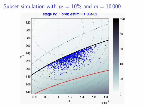
❍ We consider a cantilever beam of length L = 6 m, withuniformly distributed load (Rajashekhar & Ellingwood, 1993).

http://en.wikipedia.org/wiki/File:Beam1svg.svg

❍ The maximal deflection of the beam is

f (x1, x2) =3 L4

2 E

x1

x32

,

with x1 the load per unit area and x2 the depth.

❍ Young’s modulus: E = 2.6 104 MPa.

Example : deflection of a cantilever beam

❍ We assume an imperfect knowledge of x1 and x2 :

◮ X1 ∼ N (

µ1, σ21

)

, µ1 = 10−3 MPa, σ1 = 0.2 µ1,

◮ X2 ∼ N(

µ2, σ22

)

, µ2 = 300 mm, σ2 = 0.1 µ2.

◮ truncated independent Gaussian variables.

Example : deflection of a cantilever beam

❍ We assume an imperfect knowledge of x1 and x2 :

◮ X1 ∼ N (

µ1, σ21

)

, µ1 = 10−3 MPa, σ1 = 0.2 µ1,

◮ X2 ∼ N(

µ2, σ22

)

, µ2 = 300 mm, σ2 = 0.1 µ2.

◮ truncated independent Gaussian variables.

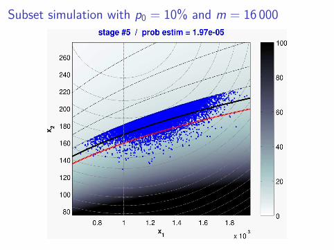
❍ A failure occurs when f (X1, X2) > u = L/325.

◮ Reference value: α ≈ 3.94 10−6,

◮ obtained by MC with m = 1010 (⇒ δ ≈ 0.5%).

❍ Note: our beam is thicker than the one of Rajashekhar &Ellingwood to make α smaller !

Subset simulation with p0 = 10% and m = 16 000

Subset simulation with p0 = 10% and m = 16 000

Subset simulation with p0 = 10% and m = 16 000

Subset simulation with p0 = 10% and m = 16 000

Subset simulation with p0 = 10% and m = 16 000

Subset simulation with p0 = 10% and m = 16 000

Subset simulation with p0 = 10% and m = 16 000

Subset simulation with p0 = 10% and m = 16 000

Subset simulation with p0 = 10% and m = 16 000

Subset simulation with p0 = 10% and m = 16 000

Subset simulation with p0 = 10% and m = 16 000

Subset simulation with p0 = 10% and m = 16 000

Subset simulation with p0 = 10% and m = 16 000

Subset simulation with p0 = 10% and m = 16 000

Subset simulation with p0 = 10% and m = 16 000

Subset simulation with p0 = 10% and m = 16 000

Subset simulation with p0 = 10% and m = 16 000

And now... Bayesian subset simulation ! (1/2)

❍ In the previous experiment, subset simulation performed

N = m + (1 − p0)(T − 1)m = 88000 evaluations of f .

where T = 6 is the number of stages.

❍ Idea : we can do much better with a Gaussian process prior.

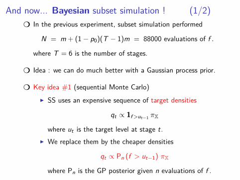
And now... Bayesian subset simulation ! (1/2)

❍ In the previous experiment, subset simulation performed

N = m + (1 − p0)(T − 1)m = 88000 evaluations of f .

where T = 6 is the number of stages.

❍ Idea : we can do much better with a Gaussian process prior.

❍ Key idea #1 (sequential Monte Carlo)

◮ SS uses an expensive sequence of target densities

qt ∝ 1f >ut−1 πX

where ut is the target level at stage t.

◮ We replace them by the cheaper densities

qt ∝ Pn (f > ut−1) πX

where Pn is the GP posterior given n evaluations of f .

And now... Bayesian subset simulation ! (2/2)

❍ Key idea #2 (adaptive sampling)

◮ At each stage t, we improve our GP model around thenext target level ut .

◮ Strategy: Stepwise Uncertainty Reduction (SUR)(Vazquez & Piera-Martinez (2007), Vazquez & Bect (2009))

◮ Other strategies could be used as well. . .(e.g., Picheny et al. (2011))

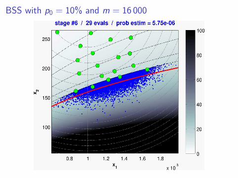
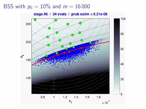
And now... Bayesian subset simulation ! (2/2)

❍ Key idea #2 (adaptive sampling)

◮ At each stage t, we improve our GP model around thenext target level ut .

◮ Strategy: Stepwise Uncertainty Reduction (SUR)(Vazquez & Piera-Martinez (2007), Vazquez & Bect (2009))

◮ Other strategies could be used as well. . .(e.g., Picheny et al. (2011))

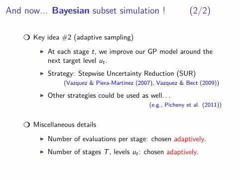
❍ Miscellaneous details

◮ Number of evaluations per stage: chosen adaptively.

◮ Number of stages T , levels ut : chosen adaptively.

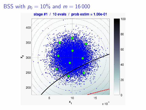
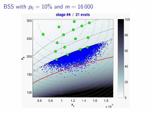
BSS with p0 = 10% and m = 16 000

BSS with p0 = 10% and m = 16 000

BSS with p0 = 10% and m = 16 000

BSS with p0 = 10% and m = 16 000

BSS with p0 = 10% and m = 16 000

BSS with p0 = 10% and m = 16 000

BSS with p0 = 10% and m = 16 000

BSS with p0 = 10% and m = 16 000

BSS with p0 = 10% and m = 16 000

BSS with p0 = 10% and m = 16 000

BSS with p0 = 10% and m = 16 000

BSS with p0 = 10% and m = 16 000

BSS with p0 = 10% and m = 16 000

BSS with p0 = 10% and m = 16 000

BSS with p0 = 10% and m = 16 000

BSS with p0 = 10% and m = 16 000

BSS with p0 = 10% and m = 16 000

BSS with p0 = 10% and m = 16 000

BSS with p0 = 10% and m = 16 000

BSS with p0 = 10% and m = 16 000

BSS with p0 = 10% and m = 16 000

BSS with p0 = 10% and m = 16 000

BSS with p0 = 10% and m = 16 000

BSS with p0 = 10% and m = 16 000

BSS with p0 = 10% and m = 16 000

BSS with p0 = 10% and m = 16 000

BSS with p0 = 10% and m = 16 000

BSS with p0 = 10% and m = 16 000

BSS with p0 = 10% and m = 16 000

BSS with p0 = 10% and m = 16 000

BSS with p0 = 10% and m = 16 000

BSS with p0 = 10% and m = 16 000

BSS with p0 = 10% and m = 16 000

BSS with p0 = 10% and m = 16 000

BSS with p0 = 10% and m = 16 000

BSS with p0 = 10% and m = 16 000

BSS with p0 = 10% and m = 16 000

BSS with p0 = 10% and m = 16 000

BSS with p0 = 10% and m = 16 000

BSS with p0 = 10% and m = 16 000

BSS with p0 = 10% and m = 16 000

BSS with p0 = 10% and m = 16 000

BSS with p0 = 10% and m = 16 000

BSS with p0 = 10% and m = 16 000

BSS with p0 = 10% and m = 16 000

BSS with p0 = 10% and m = 16 000

BSS with p0 = 10% and m = 16 000

Performance ?

❍ Preliminary Monte Carlo studies (PhD thesis of Ling Li, 2012).

◮ Case tests in dimensions d = 2 and d = 6.

◮ Comparison with plain subset simulation and the2SMART algorithm (Deheeger, 2007; Bourinet et al., 2011).

⇒ very significant evaluation savings(for a comparable MSE)

Performance ?

❍ Preliminary Monte Carlo studies (PhD thesis of Ling Li, 2012).

◮ Case tests in dimensions d = 2 and d = 6.

◮ Comparison with plain subset simulation and the2SMART algorithm (Deheeger, 2007; Bourinet et al., 2011).

⇒ very significant evaluation savings(for a comparable MSE)

❍ Our estimate is biased (nothing is free. . . ).

◮ Typically weakly biased in our experiments.

Performance ?

❍ Preliminary Monte Carlo studies (PhD thesis of Ling Li, 2012).

◮ Case tests in dimensions d = 2 and d = 6.

◮ Comparison with plain subset simulation and the2SMART algorithm (Deheeger, 2007; Bourinet et al., 2011).

⇒ very significant evaluation savings(for a comparable MSE)

❍ Our estimate is biased (nothing is free. . . ).

◮ Typically weakly biased in our experiments.

◮ Two sources of bias, that can be removed◮ level-adaptation bias

➥ solution: two passes,◮ Bayesian bias

➥ solution: evaluate all points at the last stage

Closing remarks

❍ Estimating small probabilities of failure on expensive computermodels is possible, using a blend of :

◮ advanced simulation techniques (here, SMC)

◮ meta-modelling (here, Gaussian process modelling)

❍ Benchmarking wrt state-of-the-art techniques

◮ work in progress

Closing remarks

❍ Estimating small probabilities of failure on expensive computermodels is possible, using a blend of :

◮ advanced simulation techniques (here, SMC)

◮ meta-modelling (here, Gaussian process modelling)

❍ Benchmarking wrt state-of-the-art techniques

◮ work in progress

❍ Open questions

◮ How well do we need do know f at intermediate stages ?

◮ How smooth should f be for BSS to be efficient ?

◮ Theoretical properties ?

References

❍ This talk is based on the paper

◮ Ling Li, Julien Bect, Emmanuel Vazquez, Bayesian Subset

Simulation : a kriging-based subset simulation algorithm for the

estimation of small probabilities of failure, Proceedings of PSAM 11

& ESREL 2012, June 25-29, 2012, Helsinki, Finland [clickme]

❍ For more information on kriging based adaptive samplingstrategies (a.k.a sequential design of experiments)

◮ Julien Bect, David Ginsbourger, Ling Li, Victor Picheny, Emmanuel

Vazquez, Sequential design of computer experiments for the

estimation of a probability of failure, Statistics and Computing,

22(3):773–793, 2012. [clickme]